impedance measurements of nonuniform ... in electromagnetics research, vol. 117, 149{164, 2011...

Progress In Electromagnetics Research, Vol. 117, 149–164, 2011

IMPEDANCE MEASUREMENTS OF NONUNIFORMTRANSMISSION LINES IN TIME DOMAIN USINGAN IMPROVED RECURSIVE MULTIPLE REFLECTIONCOMPUTATION METHOD

Y. Liu *, L. Tong, W.-X. Zhu, Y. Tian, and B. Gao

School of Automation Engineering, University of Electronic Scienceand Technology of China, Chengdu, Sichuan 611731, China

Abstract—In this paper, a recursive computation method isdeveloped to derive the multiple reflections of nonuniform transmissionlines. The true impedance profiles of the nonuniform transmission linesare then reconstructed with the help of this method. This method ismore efficient than other algorithm. To validate this method, twononuniform microstrip lines are designed and measured using Agilentvector network analyzer E8363B from 10MHz to 20 GHz with 10MHzinterval. The reflection coefficients of these nonuniform microstriplines in time domain are attained from the scattering parametersusing inverse Chirp-Z transform. The reconstructed characteristicimpedance profiles of the nonuniform lines are compared with thosereconstructed by Izydorczyk’s algorithm. The agreements of the resultsillustrate the validity of the recursive multiple reflection computationmethod in this paper.

1. INTRODUCTION

Planar microwave transmission lines such as microstrip lines andcoplanar waveguides are widely used in microwave circuits and high-speed digital circuits, for example, antenna [1], power dividers [2] andfilters [3]. The performances of microwave circuits and high-speeddigital circuits in time domain are much concerned by designers [4–10].As a basic measurement technique in time domain, the Time DomainReflectometry (TDR) is widely used to acquire the transient responseof the circuits [8, 9] in time domain. And as a basic measurementinstrument in frequency domain, Vector Network Analyzer (VNA),

Received 24 April 2011, Accepted 24 May 2011, Scheduled 1 June 2011* Corresponding author: Yu Liu ([email protected]).

150 Liu et al.

with the help of inverse Fourier transform algorithm, is also ableto obtain the time-domain response the same as TDR if sufficientbandwidth is provided [11, 12]. Therefore, the time domain responsesof microwave circuits and high-speed digital circuits can be attained byboth TDR and VNA. And the impedance profiles of the circuits thencan be calculated according to their time-domain responses. However,multiple reflections of a nonuniform transmission line always result inincorrect impedance readouts [13, 14]. The true impedance profilesneed to be reconstructed from the confusing measurement results.

Many authors have made significant contributions to the study ofreconstructing the true impedance profiles of nonuniform transmissionlines from the data acquired by TDR or VNA [13–19]. Theliterature [15] used a recursive method with only three variablesΓtable, Γopen and Γmatched. However, the processing time of thisalgorithm is in the order of o(N3), that is if the number of datadoubles, the computation time will be roughly eight times longer.The literature [16] used the extended peeling algorithm to extract thecircuit model of lossy interconnects from the TDR/T measurementdata. However, to implement this algorithm, the resistance per unitlength of the circuits must be measured by TDR firstly. Hsue andPan [13] divided the reflected wave into many time durations withequal length and decomposed the reflected wave into ‘wavefront’ and‘nonwavefront’ components, which make it intuitional to reconstructthe nonuniform transmission lines. However, the expression of thereflected wave Vr(t) in [13] and [19] is complicated and difficult torealize. Izydorczyk [20, 21] proposed an algorithm to reconstruct theimpedances of nonuniform transmission lines, which is simple and easyto use. The Izydorczyk’s algorithm used the relationship between thevoltages at the nth layer and the (n + 1)th layer and the algorithm isin the order of o(N2).

In this paper, a lattice diagram [14, 15] that is used to illustratethe process of the injected step voltage generated by TDR propagatingin a nonuniform transmission line is studied. Then a recursivealgorithm is developed to calculate the reflected wave Vr(t). Thisalgorithm calculates the voltages injected into the lattices recursivelyfrom the unit step response of the nonuniform transmission line.The response is acquired by TDR or VNA and includes multiplereflections. The true impedance profile of the transmission line canbe reconstructed with the help of this algorithm. To validate thealgorithm, two nonuniform microstrip lines are designed and measuredusing Agilent VNA E8363B from 10 MHz to 20 GHz with 10 MHzinterval. The unit step responses are attained from S11 of thecircuits using inverse Chirp-Z transform (ICZT). The reconstructed

Progress In Electromagnetics Research, Vol. 117, 2011 151

characteristic impedance profiles of the nonuniform lines are comparedwith those reconstructed by Izydorczyk’s algorithm. The agreements ofthe reconstructed results illustrate the validity of the recursive multiplereflection computation method in this paper.

2. THEORY

2.1. An Improved Recursive Method for Multiple ReflectionComputation

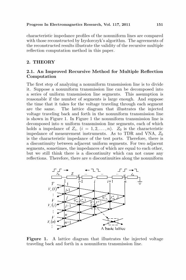
The first step of analyzing a nonuniform transmission line is to divideit. Suppose a nonuniform transmission line can be decomposed intoa series of uniform transmission line segments. This assumption isreasonable if the number of segments is large enough. And supposethe time that it takes for the voltage traveling through each segmentare the same. The lattice diagram that illustrates the injectedvoltage traveling back and forth in the nonuniform transmission lineis shown in Figure 1. In Figure 1 the nonuniform transmission line isdecomposed into n uniform transmission line segments, each of whichholds a impedance of Zi, (i = 1, 2, . . . , n). Z0 is the characteristicimpedance of measurement instruments. As to TDR and VNA, Z0

is the characteristic impedance of the test ports. Therefore, there isa discontinuity between adjacent uniform segments. For two adjacentsegments, sometimes, the impedances of which are equal to each other,but we still think there is a discontinuity which can not cause anyreflections. Therefore, there are n discontinuities along the nonuniform

Figure 1. A lattice diagram that illustrates the injected voltagetraveling back and forth in a nonuniform transmission line.

152 Liu et al.

transmission line. The TDR samples the reflected voltage at equal timeintervals, say ∆t. Let the time that it takes for the voltage travelingthrough each uniform segment be τ , therefore, ∆t is equal to 2τ . In theprocedure of construction, which is illustrated in Section 2.2, the reflectvoltages are sampled by TDR with equal time interval. If the reflectvoltages at the test port are known, the lattice diagram in Figure 1are established. Therefore, the nonuniform transmission lines are notdivided actually.

A basic lattice that is also called a cell [16] is defined in Figure 1.Let i denote the ith discontinuity and j denote the jth time interval, inother words, the time of j∆t. All lattices in Figure 1 are indexed withi and j. The voltage injected into the lattice (i, j) can be denoted as(V L

i,j , V Ri,j), where V L

i,j denotes the voltage that injected into the lattice(i, j) from its left lattice and V R

i,j denotes the voltage that injected intothe lattice (i, j) from its right lattice. It is clear in Figure 1 that theleft lattice and the right lattice of lattice (i, j) are lattice (i− 1, j) andlattice (i + 1, j − 1) respectively. As shown in Figure 1, part of V L

i,j

is reflected back to the left side by the ith discontinuity and the restpasses through. Just as V L

i,j , part of V Ri,j is reflected back to the right

side and the rest passes through and travels to the test port.Therefore, the relationship of the lattices can be determined. For

2 ≤ i < n and j ≥ 2, the voltage V Li,j that is injected into the lattice

(i, j) contains two parts: the first part is portion of V Li−1,j that travels

through lattice (i − 1, j) and the other is portion of V Ri−1,j that is

reflected back by the (i − 1)th discontinuity. Therefore, V Li,j can be

expressed by (1a). V Ri,j can be derived in the same way, just shown

in (1b).

V Li,j = Ti−2,i−1V

Li−1,j + Γi−1,i−2V

Ri−1,j (1a)

V Ri,j = Γi,i+1V

Li+1,j−1 + Ti+1,iV

Ri+1,j−1 (1b)

where Ti,i+1 and Ti+1,i are the transmission coefficients; Γi,i+1 andΓi+1,i are the reflection coefficients between Zi and Zi+1. Γi,i+1, Γi+1,i,Ti,i+1 and Ti+1,i are defined as follows.

Γi,i+1 =Zi+1 − Zi

Zi+1 + Zi= −Γi+1,i (2a)

Ti,i+1 = 1 + Γi,i+1 (2b)Ti+1,i = 1 + Γi+1,i (2c)

For the lattices such that i = 1 and j ≥ 2, the voltage injected intothe lattices from left side is generated by TDR and remains constant,


therefore

V Li,j = V (3a)

V Ri,j = Γi,i+1V

Li+1,j−1 + Ti+1,iV

Ri+1,j−1 (3b)

where the value of V in (3a) and (6a) which is shown later is themagnitude of the step voltage generated by TDR. To normalize thereflected voltage, the value of V is assigned to be 1 V.

For the lattices such that 2 ≤ i < n and j = 1, there are novoltages injecting into their left lattices indexed with i− 1 and j fromthe right sides and there are no right lattices indexed with i + 1 andj − 1. Therefore, (1a) and (1b) are rewritten as follows.


Li−1,j (4a)

V Ri,j = 0 (4b)

For the lattices such that i = n and j ≥ 2, there are no rightlattices which are indexed with i+1 and i− 1. Therefore, V L

i,j and V Ri,j

are represented as follows.


Li−1,j + Γi−1,i−2V

Ri−1,j (5a)

V Ri,j = 0 (5b)

For the lattice such that i = 1 and j = 1,

V Li,j = V (6a)

V Ri,j = 0 (6b)

And for i > n and j ≥ 1, the lattices indexed with i and j areviewed as ‘virtual’ lattices and V L

i,j and V Ri,j are assigned to be zero,

which may be useful for programming.The analysis above can be summarized by the equations as follows.

V Li,j =

Ti−2,i−1VLi−1,j , 2 ≤ i ≤ n, j = 1

Ti−2,i−1VLi−1,j + Γi−1,i−2V

Ri−1,j , 2 ≤ i ≤ n, j ≥ 2

1, i = 1, j ≥ 10, otherwise

(7)

V Ri,j =

Γi,i+1V

Li+1,j−1 + Ti+1,iV

Ri+1,j−1, 1 ≤ i < n, j ≥ 2

0, otherwise(8)

The reflected voltage measured by TDR at the time of j∆t canbe expressed by

Vr(j) = T1,0VR1,j + Γ0,1V

L1,j (9)

where j = 1, 2, 3, . . ..

154 Liu et al.

The process of multiple reflection computation is to calculate thereflect voltages at the test port according to the impedances of theuniform line segments. But by contrast, the process of impedancereconstruction is to obtain the impedance of the uniform line sectionsunder the condition that Vr is measured by TDR or VNA.

2.2. Impedance Reconstruction

For i = 1, the reflected coefficient Γ0,1 and impedance Z1 can beobtained directly from the measured data.

Γ0,1 = Vr(1) (10)

Z1 = Z01 + Γ0,1

1− Γ0,1(11)

The reflected voltage Vr(t) in literature [13] was decomposedinto ‘wavefront’ and ‘nonwavefront’ components and the reflectioncoefficient Γi−1,i between Zi−1 and Zi such that i ≥ 2 was expressedas follows [13].

Γi−1,i =Vr(i)− Vref (nonwavefront, i)

j=i−1∏

j=1

Tj−1,j

j=i−1∏

j=1

Tj,j−1

=Vr(i)− Vref (nonwavefront, i)

j=i−1∏

j=1

(1− Γ2j−1,j)

(12)

Therefore, the characteristic impedance Zi of the ith uniform segmentcan be calculated according to Zi−1 and Γi−1,i, as shown in (13).

Zi = Zi−11 + Γi−1,i

1− Γi−1,i(13)

The term Vref (nonwavefront, i) in (12) is the reflected voltage thatexperiences multiple reflection processes at the discontinuities formedby Z0, Z1, . . . , Zi−1 at the time of i∆t. If Z0, Z1, . . . , Zi−1 are known,Vref (nonwavefront, i) can be calculated by (7)∼ (9) recursively.

The impedances Z2, Z3, . . . , Zn then can be figured out accordingto (11)∼ (13) iteratively with the help of the recursive multiplereflection algorithm proposed in Section 2.1.


3. EXPERIMENTS AND RESULTS

3.1. Circuits Design

To certify the multiple reflection computation method, two nonuniformmicrostrip lines are designed. The size of the circuit boards and thesignal lines are shown in Figures 2 and 3, respectively. The impedanceof the microstrip line in Figure 2 is step change and that of themicrostrip line in Figure 3 is gradual change. To make sure those linescan be connected to the coaxial ports of the vector network analyzer,two location holes are designed at each side of the circuit boards.Two launchers are used in order to connect the circuits under test tovector network analyzer. The substrate of the both nonuniform linesis RO4350B, of which the relative dielectric constant and loss tangentare 3.48 and 0.004 respectively. The thickness of the substrate is 30 miland that of the strips is 0.7 mil. The characteristic impedances of theuniform transmission line sections are computed according to [22] andshown in Table 1.

(a)

(b)

Figure 2. Nonuniform microstrip transmission line with coaxial-to-microstrip launchers. The impedance is step change. (a) Widths andlengths of the strip line sections. (b) The designed circuit board withlaunchers.

156 Liu et al.

(a)

(b)

Figure 3. Nonuniform microstrip transmission line with coaxial-to-microstrip launchers. The impedance is gradual change. (a) Widthsand lengths of the strip line sections. (b) The designed circuit boardwith launchers.

Table 1. Characteristic impedances of uniform microstrip line sectionswith different widths. The thickness of the strips is 0.7mil.

Strip Width (mil) 66 220 450Impedance (Ω) 50.6 21.3 11.6

3.2. Reconstruction Results

The microstrip lines in Figures 2 and 3 are measured from 10 MHz to20GHz with 10 MHz interval via Agilent vector network analyzer PNAE8363B. Usually the unit step responses of the circuits are obtainedusing inverse Fast Fourier Transform (IFFT). To improve the resolutionof the responses of the microstrip lines in time domain, inverse Chirp-Z transform (ICZT) is used actually instead of IFFT [23]. Since theChirp-Z transform (CZT) has been realized in MATLAB as functionczt, the ICZT transform of scattering parameters of the microstriplines can be determined according to the relationship between CZT


and ICZT [24], just as (14).ICZT[X(k)] = (CZT[X∗(k)])∗ (14)

where the “∗” means complex conjugate.The unit step responses of the microstrip lines in Figures 2 and 3

can be obtained according to (15).

R(k) = ICZT[

S11(k)1− e−jk(2π/(N+1))

](15)

where k = 0, 1, 2, . . . , N , and N is the number of S11. The value ofS11(k)

1− e−jk(2π/(N+1))

at k = 0 is obtained by extrapolating.The hanning window [25] is used to smooth the results when

employing ICZT to compute the unit step response. The unit stepresponses are actually corresponding to the reflection coefficients ofthe microstrip lines measured by TDR. Therefore the impedances ofthe microstrip lines can be derived according to TDR principle shownin (16).

Z = Z0 · 1 + ρ

1− ρ(16)

where ρ is the reflection coefficient of the device under test in timedomain and Z0 is the characteristic impedance of the test port of TDR.

The reflection coefficients of the two nonuniform lines in Figures 2and 3 are shown in Figure 4. To ensure the resolution in time domain,the time interval is set 1.25 ps and the data number is 2000. If theincident voltage V which is shown in (3a), is assumed to be 1V, thereflection coefficient is the same as the reflected voltage Vr attained byTDR. The impedances of the nonuniform microstrip lines are computedfrom the corresponding reflection coefficients according to (16) and theresults are shown in Figure 5. Comparing with the data in Table 1,the impedance profiles of the microstrip lines in Figure 5 don’t reflectthe true profiles of the nonuniform transmission lines. The multiple-reflection effect is included in the data shown in Figures 4 and 5.

To get the true impedance profiles, both the reconstructionmethod in this paper and Izydorczyk’s algorithm are implemented tothe reflection coefficients in Figure 4 and the reconstructed impedanceprofiles of the nonuniform microstrip lines are shown in Figures 6 and 7.The black dashed lines represent the reconstructed characteristicimpedance profiles using the method in this paper; the green dash-dotted lines represent the reconstructed results using the Izydorczyk’salgorithm; and the blue dotted lines represent the impedance profilescomputed according to TDR principle.

158 Liu et al.

The reconstructed impedance profiles agree with those computedaccording to the TDR principle in the first part of the traces. This isbecause the multiple reflection does not affect the impedance profiles ofthe first part. From the reconstructed characteristic impedance profilesof the microstrip lines in Figures 6 and 7, the ripples at 0.19 ns and2.19 ns in Figure 6 and those at 0.19 ns and 2.14 ns in Figure 7 are dueto mismatch of the coaxial-to-microstrip launches that are shown inFigures 2 and 3.

0 0.5 1 1.5 2 2.5Time (ns)

Reflection C

oeffic

ient

Fig.2

Fig.3

0.1

0

-0.1

-0.2

-0.3

-0.4

-0.5

-0.6

-0.7

Figure 4. Reflection coefficientsof the microstrip lines in Figures 2and 3.

0 0.5 1 1.5 2 2.50

10

20

30

40

50

60

Time (ns)

Fig.2

Fig.3

Impedance (

Ω)

Figure 5. Impedance profiles ofthe nonuniform microstrip linesbefore reconstruction. The tracesare calculated according to TDRprinciple.

0 0.5 1 1.5 2 2.5

10

20

30

40

50

60

Time (ns)

Impedance(Ω

)

Method in this paper

No reconstruction

Izydorczyk method

Figure 6. Comparison of theimpedance profile of the mi-crostrip line in Figure 2 beforeand after reconstruction.

0 0.5 1 1.5 2 2.510

15

20

25

30

35

40

45

50

55

Time (ns)

Imp

ed

an

ce

(Ω)

Method in this paper

No reconstruction

Izydorczyk method

Figure 7. Comparison of theimpedance profile of the mi-crostrip line in Figure 3 beforeand after reconstruction.


Comparing with the impedance profiles reconstructed by themethod in this paper and the Izydorczyk’s algorithm, the consistencyof the results validates the method in this paper.

3.3. Discussion

To make the recursive multiple reflection computation algorithm in (7)and (8) more efficient, the recursive algorithm of multiple reflectioncomputation is realized using iterative procedure. The pseudocodeof the multiple reflection computation and impedance reconstructionprocedures is illustrated in Appendix A. The processing time of thealgorithm is in the order of o(N2), namely if the number of uniformline segments becomes 2N from N , the computation time will beroughly four times longer. The Izydorczyk algorithm in literatures [20]and [21] is also in the order of o(N2). Comparing with o(Nb(N +1)2 − N − 1c) which can be expressed by o(N3) in literature [15],the multiple reflection computation algorithm in this paper andIzydorczyk’s algorithm are more efficient. The time consumption of themethod in this paper and Izydorczyk’s algorithm for different numbersof data are compared in Table 2. The computation time in Table 2 maychange slightly for different programmers. The results in Table 2 showthat the method in this paper is faster than Izydorczyk’s algorithm.

In Figure 6, the reconstructed impedance profile after t =1.7 ns, and that in Figure 7 after t = 1.9 ns are not recoveredtotally from the raw reflection coefficients according to Table 1.To fully understand the multiple reflection computation algorithm,the characteristic impedance profiles of the nonuniform lines arereconstructed again according to the reflection coefficients in timedomain measured from the both ports of each circuit board. Thetwo impedance profiles of each microstrip lines are compared andshown in Figures 8 and 9, respectively. In Figure 8, the dash-dottedline represents the characteristic impedance which is reconstructedaccording to the reflection coefficients in time domain measured fromprot 2 (the right port in Figure 2). The dash-dotted impedance profile

Table 2. Computation time comparison for different data points(CPU: AMD Sempron (tm) 3000+, 1.61 GHz. DDR 896 MB). Thetime may change for different computers and different programmers.

Data Number 2000 5000 10000Method in this paper 104ms 319 ms 993 msIzydorczyk algorithm 114 ms 408 ms 1990 ms

160 Liu et al.

0 0.5 1 1.5 2 2.510

15

20

25

30

35

40

45

50

55

Time (ns)

Measured from port 1


Impedance (

Ω)

Figure 8. Impedance profiles ofthe microstrip line in Figure 2after reconstruction. The tracesare figured out according to coef-ficients from the two ports of thecircuit respectively.

0 0.5 1 1.5 2 2.510

15

20

25

30

35

40

45

50

55

Time (ns)



Impedance (

Ω)

Figure 9. Impedance profiles ofthe microstrip line in Figure 3after reconstruction. The tracesare figured out according to coef-ficients from the two ports of thecircuit respectively.

after t = 1.7 ns is also not recovered totally. This situation also happensin Figure 9.

In this paper, the relationship of transmission coefficient T and thereflection coefficient Γ between adjacent uniform sections is defined as

T = 1 + Γ (17)

In (17) the loss of the nonuniform transmission lines is not considered.This relationship is also used in [13] and [15]. However, the circuitsin the experiments are not entirely lossless. The loss tangent of thesubstrate RO4350B is 0.004. The dielectric loss makes the differencesbetween the reconstructed results and computed results in Table 1.Besides, the conductor loss and radiation loss [26] of the circuits alsoaffect the process of true impedance profile reconstruction. Therefore,as well as [13] and [15], the recursive algorithm for multiple reflectioncomputation is only suitable for lossless and low lossy nonuniformtransmission lines.

4. CONCLUSION

In this paper, an explicit and effective recursive method for multiplereflection computation is present. This recursive algorithm is realizedusing iterative procedure and the processing time of this algorithm is inthe order of o(N2). In TDR measurements, to improved the resolution


in time domain, more data are need. This algorithm is especially usefulin this situation.

ACKNOWLEDGMENT

This work is supported by State Key Laboratory of Remote SensingScience, Jointly Sponsored by the Institute of Remote SensingApplications of Chinese Academy of Sciences and Beijing NormalUniversity.

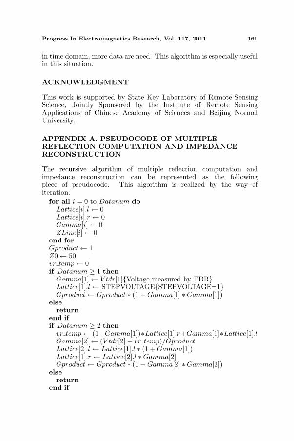
APPENDIX A. PSEUDOCODE OF MULTIPLEREFLECTION COMPUTATION AND IMPEDANCERECONSTRUCTION

The recursive algorithm of multiple reflection computation andimpedance reconstruction can be represented as the followingpiece of pseudocode. This algorithm is realized by the way ofiteration.

for all i = 0 to Datanum doLattice[i].l ← 0Lattice[i].r ← 0Gamma[i] ← 0ZLine[i] ← 0

end forGproduct ← 1Z0 ← 50vr temp ← 0if Datanum ≥ 1 then

Gamma[1] ← V tdr[1]Voltage measured by TDRLattice[1].l ← STEPVOLTAGESTEPVOLTAGE=1Gproduct ← Gproduct ∗ (1−Gamma[1] ∗Gamma[1])

elsereturn

end ifif Datanum ≥ 2 then

vr temp ← (1−Gamma[1])∗Lattice[1].r+Gamma[1]∗Lattice[1].lGamma[2] ← (V tdr[2]− vr temp)/GproductLattice[2].l ← Lattice[1].l ∗ (1 + Gamma[1])Lattice[1].r ← Lattice[2].l ∗Gamma[2]Gproduct ← Gproduct ∗ (1−Gamma[2] ∗Gamma[2])

elsereturn

end if

162 Liu et al.

for i = 3 to Datanum doLattice[i].l ← Lattice[i− 1].l ∗ (1 + Gamma[i− 1])Lattice[i−1].l ← Lattice[i−2].l∗(1+Gamma[i−2])+Lattice[i−2].r ∗ (−Gamma[i− 2])for k = i− 2 to 2 do

Lattice[k].r ← Gamma[k+1]∗Lattice[k+1].l+(1−Gamma[k+1]) ∗ Lattice[k + 1].rLattice[k].l ← (1 + Gamma[k − 1]) ∗ Lattice[k − 1].l +(−Gamma[k − 1]) ∗ Lattice[k − 1].r

end forLattice[1].r ← Lattice[2].l ∗ Gamma[2] + Lattice[2].r ∗ (1 −Gamma[2])vr temp ← (1−Gamma[1])∗Lattice[1].r+Gamma[1]∗Lattice[1].lGamma[i] ← (V tdr[i]− vr temp)/GproductGproduct ← Gproduct ∗ (1−Gamma[i] ∗Gamma[i])Dincrese ← Lattice[i].l ∗Gamma[i]Lattice[i− 1].r ← Lattice[i− 1].r + Dincresefor k = i− 2 to 1 do

Dincrese ← Dincrese ∗ (1−Gamma[k + 1])Lattice[k].r ← Lattice[k].r + Dincrese

end forend forZLine[0] ← Z0for i = 1 to Datanum do

ZLine[i] ← (1 + Gamma[i])/(1−Gamma[i]) ∗ ZLine[i− 1]end for

REFERENCES

1. Lin, D.-B., I.-T. Tang, and Y.-Y. Chang, “Flower-like CPW-FEDmonopole antenna for quad-band operation of mobile handsets,”Journal of Electromagnetic Waves and Applications, Vol. 23,Nos. 17–18, 2271–2278, 2009.

2. Wang, W., C. Liu, L. Yan, and K. Huang, “A novel powerdivider based on dual-composite right/left handed transmissionline,” Journal of Electromagnetic Waves and Applications, Vol. 23,Nos. 8–9, 1173–1180, 2009.

3. Fallahzadeh, S. and M. Tayarani, “A new microstrip UWBbandpass filter using defected microstrip structures,” Journal ofElectromagnetic Waves and Applications, Vol. 24, No. 7, 893–902,2010.

4. Zhang, G.-H., M. Xia, and X.-M. Jiang, “Transient analysis ofwire structures using time domain integral equation method with


exact matrix elements,” Progress In Electromagnetics Research,Vol. 92, 281–298, 2009.

5. Sharma, R. Y., T. Chakravarty, and A. B. Bhattacharyya,“Transient analysis of microstrip-like interconnections guarded byground tracks,” Progress In Electromagnetics Research, Vol. 82,189–202, 2008.

6. Khalaj-Amirhosseini, M., “Analysis of nonuniform transmissionlines using the equivalent sources,” Progress In ElectromagneticsResearch, Vol. 71, 95–107, 2007.

7. Sheen, D. and D. Shepelsky, “Uniqueness in the simultaneousreconstruction of multiparameters of a transmission line,” ProgressIn Electromagnetics Research, Vol. 21, 153–172, 1999.

8. Navarro, L., E. Mayevskiy, and T. Chairet, “Application oflaunch point extrapolation technique to measure characteristicimpedance of high frequency cables with TDR,” DesignConference, 2009.

9. Chen, S.-D. and C.-K. C. Tzuang, “Characteristic impedance andpropagation of the first higher order microstrip mode in frequencyand time domain,” IEEE Transactions on Microwave Theory andTechniques, Vol. 50, No. 5, 1370–1379, May 2002.

10. Xie, H., J. Wang, D. Sun, R. Fan, and Y. Liu, “Spice simulationand experimental study of transmission lines with TVSs excitedby EMP,” Journal of Electromagnetic Waves and Applications,Vol. 24, Nos. 2–3, 401–411, 2010.

11. Ostwald, O., “Time domain measurement using vector networkanalyzer ZVR,” ZVR Application Note, May 1998.

12. Agilent Technologies, “Time domain analysis using a networkanalyzer,” Application Note, 1287-12, 2007.

13. Hsue, C.-W. and T.-W. Pan, “Reconstruction of nonuniformtransmission lines from time-domain reflectometry,” IEEETransactions on Microwave Theory and Techniques, Vol. 45, No. 1,32–38, January 1997.

14. TDA Systems, “PCB interconnect characterization from TDRmeasurements,” Application Note, 1999.

15. De Padua Moreira, R. and L. R. A. X. de Menezes, “Direct synthe-sis of microwave filters using inverse scattering transmission-linematrix method,” IEEE Transactions on Microwave Theory andTechniques, Vol. 48, No. 12, 2271–2276, 2000.

16. Jong, J. M., V. K. Tripathi, L. A. Hayden, and B. Janko,“Lossy interconnect modeling from TDR/T measurements,” IEEE3rd Topical Meeting on Electrical Performance of Electronic

164 Liu et al.

Packaging, 133–135, 1994.17. Jaggard, D. L. and P. V. Frangos, “The electromagnetic inverse

scattering problem for layered dispersionless dielectrics,” IEEETransactions on Antennas and Propagation, Vol. 35, No. 8, 934–946, 1987.

18. Lin, C. J., C. C. Chiu, S. G. Hsu, and H. C. Liu, “A novel modelextraction algorithm for reconstruction of coupled transmissionlines in high-speed digital system,” Journal of ElectromagneticWaves and Applications, Vol. 19, No. 12, 1595–1609, 2005.

19. Gu, Q. and J. A. Kong, “Transient analysis of single and coupledlines with capacitively-loaded junctions,” IEEE Transactions onMicrowave Theory and Techniques, Vol. 34, No. 9, 952–964, 1986.

20. Izydorczyk, J., “Comments on “Time-domain reflectometry usingarbitrary incident waveforms”,” IEEE Transactions on MicrowaveTheory and Techniques, Vol. 51, No. 4, 1296–1298, 2003.

21. Izydorczyk, J., “Microwave time domain reflectometry,” Electron-ics Letters, Vol. 41, No. 15, 848–849, 2005.

22. Pozer, D. M., Microwave Engineering, 3rd edition, John Wiley &Sons, Inc, 2005.

23. Yiding, W., W. Yirong, and H. Jun, “Application of inverseChirp-Z transform in wideband radar,” IEEE 2001 InternationalGeoscience And Remote Sensing Symposium, Vol. 4, 1617–1619,2001.

24. Frickey, A., “Using the inverse Chirp-Z transform for time-domain analysis of simulated radar signals,” Proceedings of the5th International Conference on Signal Processing Applicationsand Technology, 1366–1371, 1995.

25. Harris, F. J., “On the use of windows for harmonic analysis withthe discrete fourier transform,” Proceedings of the IEEE, Vol. 66,No. 1, 51–83, 1978.

26. Faraji-Dana, R. and R. L. Chow, “The current distribution andac resistance of a microstrip structure,” IEEE Transactions onMicrowave Theory and Techniques, Vol. 38, No. 9, 1268–1277,1990.

impedance measurements of nonuniform ... in electromagnetics research, vol. 117, 149{164, 2011...

Documents