a heuristic for mining association rules in polynomial...

1

A Heuristic for Mining Association Rules In Polynomial Time*

E. YILMAZ

General Electric Card Services, Inc. A unit of General Electric Capital Corporation

1600 Summer Street, MS 1040-3029C, Stamford, CT, 06927, U.S.A. [email protected]

E. TRIANTAPHYLLOU Department of Industrial and Manufacturing Systems Engineering

Louisiana State University, 3128 CEBA Building, Baton Rouge, LA, 70803, U.S.A. Email: [email protected] Web: http://www.imse.lsu.edu/vangelis

J. CHEN Department of Computer Science

Louisiana State University, 298 Coates Hall, Baton Rouge, LA, 70803, U.S.A.

T. W. LIAO Department of Industrial and Manufacturing Systems Engineering

Louisiana State University, 3128 CEBA Building, Baton Rouge, LA, 70803, U.S.A.

(Last Revision: April 2, 2001) Abstract: Mining association rules from databases has attracted great interest because of its potentially very practical applications. Given a database, the problem of interest is how to mine association rules (which could describe patterns of consumers’ behaviors) in an efficient and effective way. The databases involved in today’s business environment can be very large. Thus, fast and effective algorithms are needed to mine association rules out of large databases. Previous approaches may cause an exponential computing resource consumption. A combinatorial explosion occurs because existing approaches exhaustively mine all the rules. The proposed algorithm takes a previously developed approach, called the Randomized Algorithm 1 (or RA1), and adapts it to mine association rules out of a database in an efficient way. The original RA1 approach was primarily developed for inferring logical clauses (i.e., a Boolean function) from examples. Numerous computational results suggest that the new approach is very promising. Key words: Data mining, association rules, algorithm analysis, the One Clause At a Time (OCAT) approach, randomized algorithms, heuristics, Boolean functions. *: Corresponding Author: Dr. Evangelos Triantaphyllou

Complete reference information:Complete reference information: Yilmaz, E., E. Triantaphyllou, J. Chen, and T.W. Liao, (2003), “A Heuristic “A Heuristic for Mining Association Rules In Polynomial Time,”for Mining Association Rules In Polynomial Time,” Computer and Mathematical Modelling, No. 37, pp. 219-233.

2

1. INTRODUCTION Mining of association rules from databases has attracted great interest because of its

potentially very useful applications. Association rules are derived from a type of analysis that extracts

information from coincidence [1]. Sometimes called “market basket” analysis, this methodology

allows a data analyst to discover correlations, or co-occurrences of transactional events. In the classic

example, consider the items contained in a customer’s shopping cart on any one trip to the grocery

store. Chances are that the customer’s own shopping patterns tend to be internally consistent, and that

he/she tends to buy certain items on certain days, for example milk on Mondays and beer on Fridays.

There might be many examples of pairs of items that are likely to be purchased together. For instance,

one might always buy champagne and strawberries together on Saturdays, although one only rarely

purchases either of these items separately. This is the kind of information the store manager could use

to make decisions about where to place items in the store so as to increase sales. This information can

be expressed in the form of association rules. From the example given above, the manager might

decide to place a special champagne display near the strawberries in the fruit section on the weekends

in the hope of increasing sales.

Purchase records can be captured by using the bar codes on the products. The technology to

read them has enabled businesses to efficiently collect vast amounts of data, commonly known as

“market basket data” [2]. Typically, a purchase record contains the items bought in a single

transaction, and a database may contain many such transactions. Analyzing such databases by

extracting association rules may offer some unique opportunities for businesses to increase their sales,

since such association rules can be used in designing effective marketing strategies. The sizes of the

databases involved can be very large. Thus, fast and effective algorithms are needed to mine

association rules out of them.

For a more formal definition of association rules, some notation and definitions are introduced

as follows. Let I = {A1, A2, A3, …, An} be the set with the names of the items (also called attributes,

hence the notation Ai) among which association rules will be searched [2-3]. This set is often called

the item domain. Then, a transaction is a set of one or more items obtained from the set I. This

means that for each transaction T , the relation IT ⊆ holds. Let D be the set of all transactions.

Also, let X be defined as a set of some of the items in I . The set X is contained in a transaction T

if the relation TX ⊆ holds.

Using these definitions, an association rule is a relationship of the form YX ⇒ , where

IX ⊂ , IY ⊂ , and ∅=∩YX . The set X is the antecedent part, while the set Y is the

consequent part of the rule. Such an association rule holds with some confidence level denoted as

CL . The confidence level is the conditional probability (as it can be inferred from the available

3

transactions in the target database) of having the consequent part Y given that we already have the

antecedent part X. Moreover, an association rule has support S , where S is the number of

transactions in D that contain X and Y together. A frequent item set is a set of items that occur

frequently in the database. That is, their support is above a predetermined minimum support level. A

candidate item set is a set of items, possibly frequent, but not yet checked whether they meet the

minimum support criterion. The association rule analysis in our approach will be restricted to those

association rules which have only one item in the consequent part of the rule. However, a

generalization can be made easily.

Example 1.1:

Consider the following illustrative database:

=

11000111101111110000101111101000110000110110001101

D

This database is defined on five items, so { }54321 ,,,, AAAAAI = . Each row represents a

transaction. For instance, the second row represents a transaction in which only items 3A and 4A

were bought. The support of the rule 542 AAA → is equal to 3. This is true because the items 2A ,

4A , and 5A occur simultaneously in 3 transactions (i.e., the fifth, eighth, and nineth transactions).

The confidence level of the rule 542 AAA → is 100% because the number of transactions in which

2A and 4A appear together is equal to the number of transactions that 2A , 4A , and 5A appear (both

are equal to three), giving a confidence level of 100%. <

Given the previous definitions, then the problem of interest is how to mine association rules

out of a database D , that meet some pre-established minimum support and confidence level

requirements.

Mining of association rules was first introduced by Agrawal, Imielinski and Swami in [4].

Their algorithm is called AIS (which stands for Agrawal, Imielinski, and Swami). Another study used

a different approach to solve the problem of mining association rules [5]. That study presented a new

algorithm called SETM (for Set Oriented Mining). The new algorithm was proposed to mine

4

association rules by using relational operations in a relational database environment. This was

motivated by the desire to use the SQL system to compute frequent item sets.

The next study [2] received a lot more recognition than the previous ones. Three new

algorithms were presented; the Apriori, the AprioriTid, and the AprioriHybrid. The Apriori and

AprioriTid approaches are fundamentally different from the AIS and the SETM algorithms. As the

name AprioriHybrid suggests, this approach is a hybrid between the Apriori and the AprioriTid

algorithms.

Another major study in the field of mining of association rules is described in [6]. These

authors presented an algorithm called Partition. Their approach reduces the search by first computing

all frequent item sets in two passes over the database. Another major study on association rules takes a

sampling approach [7]. These algorithms make only one full pass over the database. The main idea is

to select a random sample, and use it to determine representative association rules that are very likely

to also occur in the whole database. These association rules are in turn validated in the entire database.

This paper is organized as follows. The next section presents a formal description of the

research problem under consideration. The third section starts with a brief description of the OCAT

(one clause at a time) approach that played a critical role in the development of the new approach. The

new approach is described in the second half of the third section. The fourth section presents an

extensive computational study that compared the proposed approach for the mining of association

rules with some existing ones. Finally, the paper ends with a conclusions section.

2. PROBLEM DESCRIPTION

Previous work on mining of association rules focused on extracting all conjunctive rules,

provided that these rules meet the criteria set by the user. Such criteria can be the minimum support

and confidence levels. Although previous algorithms mainly considered databases from the domain of

market basket analysis, they have been applied to the fields of telecommunication data analysis, census

data analysis, and to classification and predictive modeling tasks in general [3]. These applications

differ from market basket analysis in the sense that they contain dense data. That is, such data might

possess all or some of the following properties:

(i) Have many frequently occurring items; (ii) Have strong correlations between several items; (iii) Have many items in each record.

When standard association rule mining techniques are used (such as the Apriori approach [2]

and its variants), they may cause exponential resource consumption in the worst case. Thus, it may

take too much CPU time for these algorithms to mine the association rules. The combinatorial

explosion is a natural result of these algorithms, because they mine exhaustively all the rules that

5

satisfy the minimum support constraint as specified by the analyst. Furthermore, this characteristic

may lead to the generation of an excessive number of rules. Then, the end user will have to determine

which rules are worthwhile. Therefore, the higher the number of the derived association rules is, the

more difficult it is to review them. In addition, if the target database contains dense data, then the

previous situation may become even worse.

The size of the database also plays a vital role in data mining algorithms [7]. Large databases

are desired for obtaining accurate results, but unfortunately, the efficiency of the algorithms depends

heavily on the size of the database. The core of today’s algorithms is the Apriori algorithm [2] and

this algorithm will be the one to be compared with in this paper. Therefore, it is highly desirable to

develop an algorithm that has polynomial complexity and still being able of finding a few rules of

good quality.

3. METHODOLOGY

3.1 The One Clause At a Time (OCAT) Approach

The proposed approach is based on a heuristic, called the Randomized Algorithm 1 (or RA1)

that was developed in [8]. This heuristic infers logical clauses (Boolean functions) from two mutually

exclusive collections of binary examples. The main ideas of this heuristic are briefly described next.

Let { }nAAA ,...,, 21 be a set of n binary attributes. Also, let F be a Boolean function over

these binary attributes. That is, F is a mapping from {0, 1}n → {0, 1}. The input of the RA1 heuristic

is two sets of mutually exhaustive training examples. Each example is a vector of size n defined in

the space {0, 1}n. The training examples somehow have been classified as either positive or negative.

Then, the Boolean function to be inferred should evaluate to true (1) when it is fed with a positive

example and to false (0) when it is fed with a negative example. Hopefully, this function is an

accurate estimation of the “hidden logic” that has classified the training examples. Another goal is for

the inferred Boolean function (when it is expressed in conjunctive normal form (CNF) or disjunctive

normal form (DNF)) to have a very small, ideally minimum, number of disjunctions or conjunctions

(also known as “terms” in the literature). A Boolean function is in CNF if it is of the form:

∨∧

∈= ii

k

ja

jρ1

Similarly, a Boolean function is in DNF if it is in the form:

∧∨

∈= ii

k

ja

jρ1

6

where ia is either a binary attribute iA or its negation, iA and the variable jρ is the set of the indices

of the attributes in the thj conjunction or disjunction. As it is shown in [9] any Boolean function can

be transformed into the CNF or DNF form. Also, in [10] a simple transformation scheme is presented

for inferring CNF functions with algorithms that initially infer DNF functions and vice-versa.

In order to help fix ideas of how the RA1 algorithm operates, consider the following positive

and negative example sets, denoted as +E and −E , respectively.

== −+

011100010000111110000101

,

1001110000110010

EE

Now consider the following Boolean expression (in CNF):

( ) ( ) ( )4313242 AAAAAAA ∨∨∧∨∧∨ .

It can be easily verified that this Boolean expression correctly classifies the previous training

examples. In [11-12] the authors present a strategy called the One Clause At a Time (OCAT)

approach (see also Figure 1) for inferring a Boolean function from two classes of binary examples.

i = 0, C = ∅; {initializations}

DO WHILE −E ≠ ∅

Step 1: i ← i +1; {where i indicates the thi clause}

Step 2: Find a clause ic which accepts all members of +E while it rejects

as many members of −E as possible;

Step 3: Let −E ( ic ) be the set of members of −E which are rejected by ic ;

Step 4: Let icCC ∪← ;

Step 5: Let −E ← −E - −E ( ic );

REPEAT; Figure 1: The One Clause At a Time (OCAT) Approach,

for the CNF Case [11].

As it is indicated in Figure 1, the OCAT approach attempts to minimize the number of

CNF clauses that will finally form the target function F . A key task in the OCAT approach

is Step 2 (in Figure 1). At Step 2 a single clause is constructed. In [11] a branch-and-bound

approach is developed that infers a clause (for the CNF case) that accepts all the positive

examples while it rejects as many negative examples as possible. Later, in [8] the RA1

7

heuristic is proposed that returns a clause that now rejects many (as opposed to as many as

possible) negative examples (and still accepts all the positive examples). Next, are some

definitions that are used in these approaches and are going to be used in the new approach as

well.

C is the set of attributes in the current clause (a disjunction for the CNF case); ak an attribute such that ak ∈ A , where A is the set of the attributes 1A , 2A , …, nA and

their negations; POS (ak) the number of all positive examples in +E which would be accepted if attribute ak

were included in the current CNF clause;

NEG (ak) the number of all negative examples in −E which would be accepted if attribute ak were included in the current clause;

l the size of the candidate list; ITRS the number of times the clause forming procedure is repeated.

The RA1 algorithm is described next in Figure 2. Its time complexity is of O(D2nlogn) order

(where D is the number of transactions in the database and n is the number of items or attributes). This

follows by observing that the inner most loop requires nlogn operations when a quick sort approach is

applied for sorting the POS/NEG values. The inner most loop is repeated in order of O(E+) steps that

is the same as order O(D). Similarly, the outer loop is also of order O(D). Thus, the time complexity

of the RA1 algorithm is of order O(D2nlogn). For illustrative purposes, this algorithm is applied on the

two sets of binary vectors given earlier in this section. When the previous definitions are used, then

the following can be easily derived:

The set of the attributes (items) for these positive and negative examples is:

{ }43214321 ,,,,,,, AAAAAAAAA = }.

Therefore, the POS (ak) and NEG (ak) values are:

POS ( 1A )=2 NEG ( 1A )=4 POS ( 1A )=2 NEG ( 1A )=2




8

DO for ITRS number of iterations BEGIN

DO WHILE ( )∅≠−E

∅=C ; {initializations}

DO WHILE ( )∅≠+E

Step 1: Rank in descending order all attributes Aai∈ (where ia is either

ii

AA or ) according to their POS(i

a )/NEG( ia ) value. If NEG( ia ) =

0, then POS( ia )/NEG( ia ) = 1000 (i.e., an arbitrarily high value);

Step 2: Form a candidate list of the attributes which have the l top highest POS( ia )/NEG( ia ) values;

Step 3: Randomly choose an attribute ka from the candidate list;

Step 4: Let the set of atoms in the current clause be kaCC ∪← ;

Step 5: Let ( )kaE+ be the set of members of +E accepted when ka is

included in the current CNF clause;

Step 6: Let ( )kaEEE +++ −← ;

Step 7: Let }{k

aAA −← ;

Step 8: Calculate the new POS( ka ) values for all Aak∈ ;

REPEAT

Step 9: Let ( )CE− be the set of members of −E which are rejected by C ;

Step 10: Let ( )CEEE −−− −← ;

Step 11: Reset +E to the original value; REPEAT

END CHOOSE the final Boolean system among the previous ITRS systems that has the smallest number of clauses.

Figure 2: The RA1 Heuristic for the CNF Case [8].

By examining the previous definitions, some key observations can be made at this point.

When an attribute of high POS function value is chosen to be included in the CNF clause currently

being formed, then it is very likely that this will cause accepting some additional positive examples.

The reverse is true for atoms with a small NEG function value in terms of the negative examples.

Therefore, attributes that have high POS function values and low NEG function values are a good

choice for inclusion in the current CNF clause. This key observation leads to the following

alternatives for defining an evaluative criterion for Step 1 in Figure 2 for including a new atom in the

CNF clause under consideration: POS/NEG, or POS-NEG, or some type of a weighted version of these

9

two expressions. In [8] it was shown through some empirical experiments that the POS/NEG ratio is

an effective evaluative criterion, since it is very likely to lead to Boolean functions with few clauses.

In terms of the previous illustrative data, the POS/NEG ratios are as follows:

( )( ) =

1

1

NEG

POS

A

A0.5

( )( ) =

1

1

NEG

POS

A

A1.0

( )( ) =

2

2

NEG

POS

A

A1.0

( )( ) =

2

2

NEG

POS

A

A0.5

( )( ) =

3

3

NEG

POS

A

A0.33

( )( ) =

3

3

NEG

POS

A

A1.0

( )( ) =

4

4

NEG

POS

A

A1.0

( )( ) =

4

4

NEG

POS

A

A0.5

Next suppose that l in Step 2, Figure 2, was chosen to be equal to 3. Then, the 3 highest

POS/NEG values for this case are: {1.0, 1.0, 1.0}. These values correspond to the attributes 1A , 2A ,

and 4A , respectively. Let 2A be the one to be randomly selected out of this candidate list. The atom

2A accepts (please note that the current CNF clause is now nil) the first and the second examples in

the +E set. This means that more attributes are required in the current CNF clause being built for all

positive examples to be accepted. Next, suppose (after the POS/NEG ratios have been recalculated)

that 4A was the second attribute to be included in the clause. Note that 2A and 4A together can accept

all the positive examples in the +E set. Therefore, the first CNF clause (i.e., ( )42 AA ∨ ) of the

Boolean expression is ready.

Next one can observe which negative examples are not rejected by this clause: this clause fails

to reject the second, third and the sixth examples in the −E set. Therefore, the updated −E set should

contain the second, third and the sixth examples from the original −E set. This process is repeated

until the −E set is empty (Figure 1), meaning that all the negative examples are rejected. By recalling

that RA1 is a randomized algorithm (it repeats the function generation task ITRS times) and thus it

does not return a deterministic solution, a Boolean expression accepting all the positive examples and

rejecting all the negative examples could be:

( ) ( ) ( )4313242 AAAAAAA ∨∨∧∨∧∨ .

10

3.2 Proposed Alterations to the RA1 Algorithm

For a Boolean expression to reveal information about associations in a database, it is more

convenient to be expressed in DNF. The first step is to select an attribute about which associations

will be sought. This attribute will form the consequent part of the desired association rules. By

selecting an attribute, the database can be partitioned into two mutual sets of records (binary vectors).

Vectors that have value equal to “1” in terms of the selected attribute, can be seen as the positive

examples. A similar interpretation holds true for records that have a value of “0” for that attribute.

These vectors will be the set of the negative examples.

Given the above way for partitioning (dichotomizing) a database of transactions, it follows that

each conjunction (logical clause or “term”) of the target function will reject all the negative examples,

while on the other hand, it will accept some of the positive examples. Of course, when all the

conjunctions are considered together, then they will accept all the positive examples.

In terms of association rules, each clause in the Boolean expression (which now is expressed

in DNF) can be thought as a set of frequent item sets. That is, such a clause forms a frequent item set.

Thus, this clause can be checked further whether it meets the preset minimum support and confidence

level criteria.

The requirement of having Boolean expressions in DNF does not mean that the RA1 algorithm

has to be altered to produce Boolean expressions in DNF. However, it will have to be altered in order

to make it compatible with mining of association rules, but its original CNF producing nature (as

described in Figure 2) will be kept as it is. As it shown in [10] if one forms the complements of the

positive and negative sets and then swaps their roles, then a CNF producing algorithm, will produce a

DNF expression (and vice-versa). The last alteration is in the CNF (or DNF) expression to swap the

logical operators ( ∧) AND and OR ( ∨ ).

Another interesting issue is to observe that the confidence level of the association rules

produced by processing frequent item sets (i.e., clauses of a Boolean expression in DNF when the

OCAT / RA1 approach is used) will always be equal to 100%. This happens because each DNF clause

rejects all the negative examples while it accepts some of the positive examples when a database with

transactions is partitioned as described above.

A critical change in the RA1 heuristic is that for deriving association rules, it should only

consider the attributes themselves and not their negations. This is not always the case, since some

authors have also proposed to use association rules with negations [13]. However, association rules

are usually defined on the attributes themselves and not on their negations.

Some changes need also to be made to the selection process of the single attribute to be

included in the clause being formed (Step 1 in Figure 2). If NEG( ia ) = 0 at Step 1, then the value of

11

the ratio POS( ia )/NEG( ia ) for that particular ia is set to be equal to 1,000 (i.e., an arbitrarily high

positive number) multiplied by the POS( ia ) value. However, the number 1,000 may still be small and

thus it should be changed according to the size of the database. There are four cases regarding the

value of the POS/NEG ratio that need to be considered when selecting an attribute. These cases are:

Case #1: Multiple attributes (items) with NEG( ia ) = 0 and equal values of the

POS( ia )/NEG( ia ) ratio.

Case #2: No attributes (items) with value NEG( ia ) = 0 exist, but when all the

attributes are ranked according to their POS( ia )/NEG( ia ) values in descending order,

then the highest POS( ia )/NEG( ia ) value occurs multiple times.

Case #3: A single attribute with NEG( ia ) = 0 exists.

Case #4: There are no attributes with NEG( ia ) = 0, but when all the attributes are

ranked according to their POS( ia )/NEG( ia ) values in descending order, then the

highest POS( ia )/NEG( ia ) value occurs only once.

For cases #1 and #2, the attribute to be included in the clause being formed is randomly

selected among the candidates. The candidates for case #1 are those attributes with NEG( ia ) = 0 and

equal values of POS( ia ). The candidates for case #2, on the other hand, are those attributes that share

the same POS( ia )/NEG( ia ) value (and this is the highest value). For cases #3 and #4 there is no need

for a random selection process, since there is a single attribute with the highest POS( ia )/NEG( ia )

value. Thus, that particular attribute is included in the clause being formed.

Furthermore, if one considers only the attributes themselves and excludes their negations, this

requirement may cause certain problems due to certain degenerative situations that could occur. These

degenerative situations occur as follows:

Degenerative Case #1: If only one item is bought in a transaction, and if that particular item is selected to be the consequent part of the association rules sought, then the +E set will have an example (i.e., the one that corresponds to that transaction) with only zero elements. Thus, the RA1 heuristic (or any variant of it) will never terminate. Hence, for simplicity it will be assumed that such degenerative transactions do not occur in our databases. Degenerative Case #2: After forming a clause, and after the −E set is updated (Step 10 in Figure 2), the new POS/NEG values may be such that the new clause may be one of those that have been already produced earlier (i.e., it is possible to have “cycling”). Degenerative Case #3: A newly generated clause may not be able to reject any of the negative examples.

12

The previous is an exhaustive list of all possible degenerative situations when the original

RA1 algorithm is used. Thus, the original RA1 algorithm needs to be altered in order to avoid them.

Degenerative case #1 can be easily avoided by simply discarding all one-item transactions (which are

very rare to occur in reality any way). Degenerative cases #2 and #3 can be avoided by establishing

some upper limits on the number a Boolean function is generated without being able to reject all the

negative examples (please recall the randomized characteristic of the RA1 heuristic).

In order to mine association rules that have different consequents, the altered RA1 should be

run for each one of the attributes: 1A , 2A , …, nA . After determining the frequent item sets for each

one of these attributes, one needs to calculate the support level for each frequent item set, and check

whether the (preset) minimum support criterion is met. If it is, then the current association rule is

reported. The proposed altered RA1 (to be denoted as ARA1) heuristic is summarized in Figure 3.

Finally, it should be stated here that the new heuristic is also of time complexity O(D2nlogn) as is the

case with the original RA1 algorithm. This follows easily from a computational analysis similar to the

one described in the previous sub-section for the RA1 algorithm.

13

DO for each consequent 1A , 2A , …, nA

BEGIN Form the +E and −E sets according to the presence or absence of the current iA attribute.

Calculate the initial POS and NEG values. Let A = { 1A , 2A , …, nA }.

DO WHILE ( )∅≠−E

∅=C ; {initializations}

START1: DO WHILE ( )∅≠+E

Step 1: Rank in descending order all attributes Aai∈ (where ia is the attribute

currently under consideration) according to their POS( ia )/NEG( ia ) value.

If NEG( ia ) 0= , then POS( ia )/NEG( ia ) = 1,000 xPOS( ia );

Step 2: Evaluate the current POS/NEG case; Step 3: Choose an attribute ka accordingly;

Step 4: Let the set of atoms in the current clause be }{ kaCC ∪← ;

Step 5: Let ( )kaE+ be the set of members of +E accepted when ka is included

in the current CNF clause;

Step 6: Let ( )kaEEE +++ −← ;

Step 7: Let }{k

aAA −← ;

Step 8: Calculate the new POS( ka ) values for all Aak

∈ ;

Step 9: If ∅=A (i.e., checking for failure case #1), then go to START1; REPEAT

Step 10: Let ( )CE− be the set of members of −E which are rejected by C ;

Step 11: If ( ) ∅=− CE , determine the failure case (i.e., case #2, or #3). Check whether the corresponding counter has hit the preset limit. If yes, then go to START1;

Step 12: Let ( )CEEE −−− −← ; Step 13: Calculate the new NEG values; Step 14: Let C be the antecedent and iA be the consequent of the rule.

Check the candidate rule iAC → for minimum support. If it meets the

minimum support level criterion, then output the rule;

Step 15: Reset the +E set (i.e., select the examples which have iA equal to “1”

and store them in set +E ); REPEAT

END

Figure 3: The Proposed Altered Randomized Algorithm 1 (ARA1) for Mining Association Rules (for the CNF Case).

14

4. COMPUTATIONAL EXPERIMENTS

In order to compare the altered RA1 (ARA1) heuristic with some of the existing association

rule methods, we applied them on several synthetic databases that were generated by using the data

generation programs described in [2]. The web address (URL) of these codes is:

http://www.almaden.ibm.com/cs/quest/syndata.html. These databases contain transactions that

would reflect the real world, where people tend to buy sets of certain items together.

Several databases were used in making these comparisons. The sizes of the databases used are

as follows:

Database #1: 1,000 items with 100,000 transactions (the min support was set to 250). Database #2: 1,000 items with 10,000 transactions (the min support was set to 25). Database #3: 500 items with 5,000 transactions (the min support was set to 12). Database #4: 500 items with 4,500 transactions (the min support was set to 11). Database #5: 500 items with 4,000 transactions (the min support was set to 10).

The first results are from the densest databases used in [2], that is, database #1. The Apriori

algorithm was still in the process of generating the frequent item sets of length 2 after 80 hours 22

minutes and 8 seconds when database #1 was used. Therefore, the experiment with the Apriori

algorithm was aborted. However, the ARA1 algorithm completed mining the very same database in

only 44 hours 22 minutes and 1 second. The ARA1 algorithm mined a single rule for each one of the

following support levels: 259, 263, 308, 441, 535, 623, 624, 756, 784, 984, and 1,093. All the

experiments were run on an IBM 9672/R53 computer. This processor is a 10-engine box with each

engine being rated at 26 MIPS (millions of instructions per second).

For the experiments with database #2, however, some parallel computing techniques were

utilized for the Apriori algorithm. The frequent item sets were gathered into smaller groups, making it

possible to build the next frequent item sets in shorter time. As a result, each group was analyzed

separately, and the CPU times for each one of these jobs were added together at the end. The Apriori

algorithm completed mining this database in 59 hours 15 minutes and 3 seconds. Figure 4 illustrates

the number of rules for this case. On the other hand, the ARA1 algorithm mined database #2 in only 2

hours 54 minutes and 57 seconds. These results are depicted in Figure 5.

15

0

5,000

10,000

15,000

20,000

25,000

25 30 35 40 45 50 55 60 65 70 75 80 85 90 95 100 105 110

Support Level

Num

ber

of r

ules

min

ed

Figure 4: Histogram of the Results When the Apriori Approach Was Used on Database #2.

0

2

4

6

8

10

12

25 31 37 43 49 55 61 67 73 79 85 91 97 103 109

Support Level

Num

ber

of r

ules

min

ed

Figure 5: Histogram of Results When the ARA1 Approach Was Used on Database #2.

16

It should be noted here that the CPU times recorded for the Apriori experiments for this

research were higher than the similar results reported in [2]. For instance, it was reported in [2] that

the Apriori algorithm took approximately 500 seconds to mine database #1. That result was obtained

on an IBM RS/6000 530H workstation with a main memory of 64 MB, and running AIX 3.2. On the

other hand, for database #1, the Apriori program written for this research was in the process of

generating item sets of length 2 after 80 hours 22 minutes and 8 seconds. The only difference between

the approach taken in [2] and the one in this research is that the candidate item sets in [2] were stored

in a hash tree. Hashing is a data storage technique that provides fast direct access to a specific stored

record on the basis of a given value for some field [14].

In this research, hash trees were not used in storing candidate item sets; instead they were kept

in the main memory of the computer. This made it faster to access candidate item sets because direct

access is generally very expensive CPU-wise. It is believed that the programming techniques and the

type of the computers used in [2] are causing the CPU time difference. Additionally, the Apriori code

in this research was run under a time-sharing option, which again could make a big difference. As it

was mentioned earlier, the computer codes for the Apriori and the ARA1 algorithms were run on an

IBM 9672/R53 computer. The results obtained by using database #2 suggest that ARA1 produced a

reasonable number of rules fast. Also, these rules were of high quality, since by construction, all had a

100% confidence level.

After obtaining these results, it was decided to mine the remaining databases by also using a

commercial software, namely MineSet by Silicon Graphics. MineSet is one of the most commonly

used data mining computer packages. Unfortunately, MineSet works with transactions of a fixed

length. Therefore, the transactions were coded as zeros and ones, zeros representing that the

corresponding item was not bought, and ones representing that the corresponding item was bought.

However, this causes Mineset to mine negative association rules, too. Negative association rules are

rules based on the absence of items in the transactions, rather than the presence of them and negations

of attributes may appear in the rule structure. Another drawback of MineSet is that only a single item

is supported in both the left and the right hand sides of the rules to be mined. Also, the current version

of MineSet allows for a maximum of 512 items in each transaction. The MineSet software used for

this study was installed on a Silicon Graphics workstation, which had a CPU clock rate of 500 MHz

and a RAM of 512MB.

MineSet supports only a single item in both the left and the right hand sides of the association

rules. This suggests that MineSet uses a search procedure of also polynomial time complexity. Such

an approach would have first to count the support of each item when it is compared with every other

17

item, and store these supports in a triangular matrix of dimension n (i.e., equal to the number of

attributes).

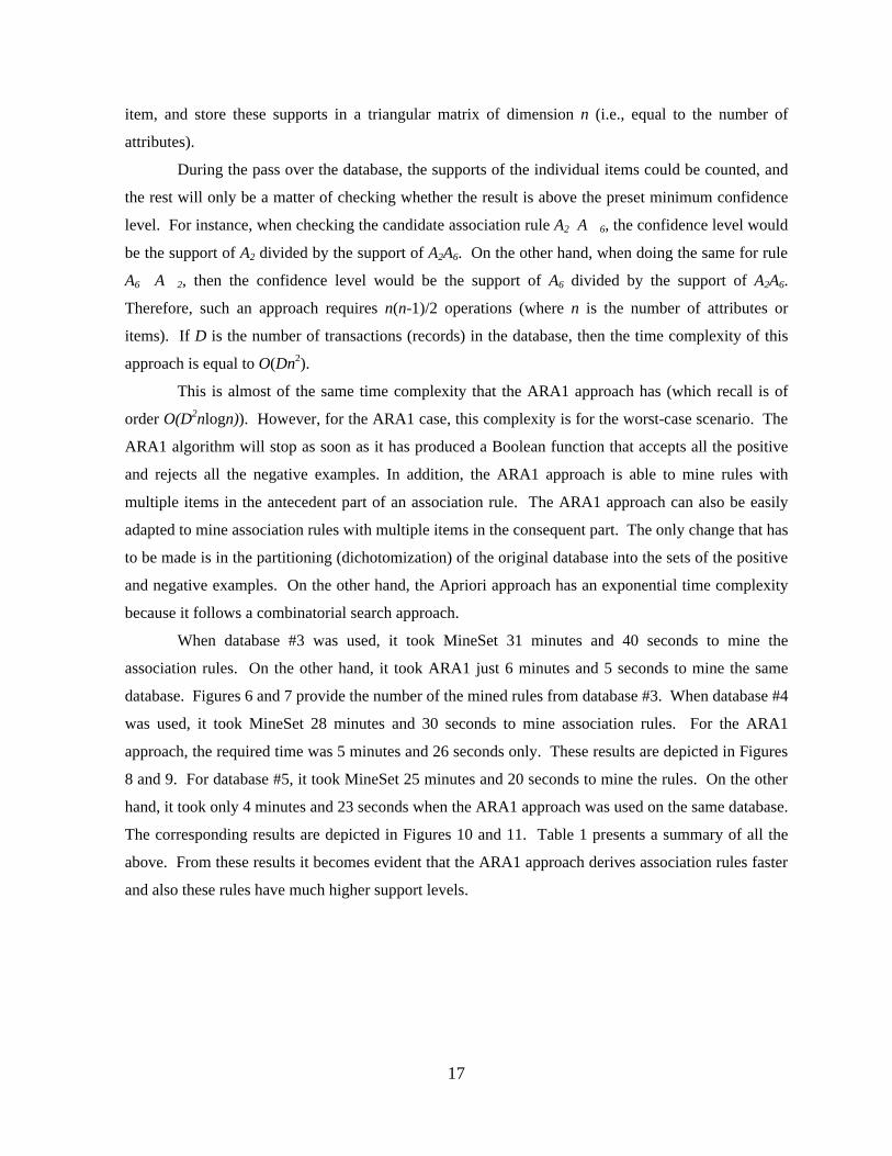
During the pass over the database, the supports of the individual items could be counted, and

the rest will only be a matter of checking whether the result is above the preset minimum confidence

level. For instance, when checking the candidate association rule A2 � A 6, the confidence level would

be the support of A2 divided by the support of A2A6. On the other hand, when doing the same for rule

A6 � A 2, then the confidence level would be the support of A6 divided by the support of A2A6.

Therefore, such an approach requires n(n-1)/2 operations (where n is the number of attributes or

items). If D is the number of transactions (records) in the database, then the time complexity of this

approach is equal to O(Dn2).

This is almost of the same time complexity that the ARA1 approach has (which recall is of

order O(D2nlogn)). However, for the ARA1 case, this complexity is for the worst-case scenario. The

ARA1 algorithm will stop as soon as it has produced a Boolean function that accepts all the positive

and rejects all the negative examples. In addition, the ARA1 approach is able to mine rules with

multiple items in the antecedent part of an association rule. The ARA1 approach can also be easily

adapted to mine association rules with multiple items in the consequent part. The only change that has

to be made is in the partitioning (dichotomization) of the original database into the sets of the positive

and negative examples. On the other hand, the Apriori approach has an exponential time complexity

because it follows a combinatorial search approach.

When database #3 was used, it took MineSet 31 minutes and 40 seconds to mine the

association rules. On the other hand, it took ARA1 just 6 minutes and 5 seconds to mine the same

database. Figures 6 and 7 provide the number of the mined rules from database #3. When database #4

was used, it took MineSet 28 minutes and 30 seconds to mine association rules. For the ARA1

approach, the required time was 5 minutes and 26 seconds only. These results are depicted in Figures

8 and 9. For database #5, it took MineSet 25 minutes and 20 seconds to mine the rules. On the other

hand, it took only 4 minutes and 23 seconds when the ARA1 approach was used on the same database.

The corresponding results are depicted in Figures 10 and 11. Table 1 presents a summary of all the

above. From these results it becomes evident that the ARA1 approach derives association rules faster

and also these rules have much higher support levels.

18

0

2

4

6

8

10

12

14

13 15 17 19 21 23 25 27 29 31 33 35 37 39 41 43Support Level

Num

ber

of m

ined

rul

es

Figure 6: Histogram of the Results When the MineSet Software Was Used on Database #3.

0

5

10

15

20

25

12 18 24 30 36 42 48 54 60 66 72 78 84 90 96 102 108 114 120

Support Level

Num

ber

of r

ules

min

ed

Figure 7: Histogram of the Results When the ARA1 Approach Was Used on Database #3.

19

0

2

4

6

8

10

12

14

16

18

20

12 14 16 20 21 24 26 28 33 35 40

Support Level

Num

ber

of r

ules

min

ed


0

5

10

15

20

25

30

11 17 23 29 35 41 47 53 59 65 71 77 83 89 95 101 107

Support Level

Num

ber

of r

ules

min

ed


20

0

2

4

6

8

10

12

14

16

18

10 12 14 16 18 20 22 24 26 28 30 32 34 36 38

Support Level

Num

ber

of r

ules

min

ed


0

5

10

15

20

25

30

10 14 18 22 26 30 34 38 42 46 50 54 58 62 66 70 74 78 82 86 90 94

Support Level

Num

ber

of r

ules

min

ed


21

Table 1: Summary of the Required CPU Times Under Each Method.

Apriori CPU (hh:mm:ss)

ARA1 CPU (hh:mm:ss)

MineSet CPU (hh:mm:ss)

Database #1 Not completed 44:22:01 N/A Database #2 59:15:03 02:54:57 N/A Database #3 N/A 00:06:05 00:31:40 Database #4 N/A 00:05:26 00:28:30 Database #5 N/A 00:04:23 00:25:20

5. CONCLUSIONS

This paper presented the developments of a new approach for deriving association rules from

databases. The new approach is called ARA1 and it is based on a previous algorithm (i.e., the RA1

approach) that was developed by one of the authors and his associates in [8]. Both the old and new

approach are randomized algorithms.

The proposed ARA1 approach produces a small set of association rules in polynomial time.

Furthermore, these rules are of high quality with 100% support levels. The 100% support level of the

derived rules is a characteristic of the way the ARA1 approach constructs association rules. The

ARA1 approach can be further extended to handle cases with less than 100% support levels. This can

be done by introducing stopping rules that terminate the appropriate loops in Figure 3. That is, to have

a predetermined lower limit (i.e., a percentage less than 100%) of the positive examples to be accepted

by each clause (in the CNF case) and also a predetermined percentage of the negative examples is

rejected instead of seeking for all the positive examples to be accepted and all the negative examples to

be rejected as is the current case.

An extensive empirical study was also undertaken. The Apriori approach and the MineSet

software by Silicon Graphics were compared with the proposed ARA1 algorithm. The computational

results demonstrated that the new approach can be both highly efficient and effective. The above

observations strongly suggest that the proposed ARA1 algorithm is very promising for mining

association rules in today’s world with the always-increasing and diverse databases.

22

REFERENCES

1. T. Blaxton and C. Westphal, Data Mining Solutions: Methods and Tools for Solving Real-World Problems, John Wiley & Sons, Inc., 186-189, New York, NY, (1998).

2. R. Agrawal and R. Srikant, Fast algorithms for mining associations rules, Proceedings of the 20th

VLDB Conference, Santiago, Chile, (1994). 3. R.J. Bayardo Jr., R. Agrawal and D. Gunopulos, Constraint-based rule mining in large, dense

databases, Proceedings of the 15th International Conference on Data Engineering, (1999). 4. R. Agrawal, T. Imielinski and A. Swami, Mining association rules between sets of items in large

databases, Proceedings of the 1993 ACM SIGMOD Conference, Washington, DC, May, (1993). 5. M. Houtsma and A. Swami, Set oriented mining of association rules, Technical Report RJ 9567,

IBM, October, (1993). 6. A. Savasere, E. Omiecinski and S. Navathe, An efficient algorithm for mining association rules in

large databases, Data Mining Group, Tandem Computers, Inc., Austin, TX, (1995). 7. H. Toivonen, Sampling large databases for association rules, Proceedings of the 22nd VLDB

Conference, Bombay, India, (1996). 8. A.S. Deshpande and E. Triantaphyllou, A greedy randomized adaptive search procedure(GRASP)

for inferring logical clauses from examples in polynomial time and some extensions, Mathematical and Computer Modelling 27, 75-99, (1998).

9. J. Peysakh, A fast algorithm to convert Boolean expressions into CNF, IBM Computer Science

RC 12913(#57971), Watson, NY, (1987). 10. E. Triantaphyllou and A.L. Soyster, A relationship between CNF and DNF systems derivable from

examples, ORSA Journal on Computing 7, 283-285 (1995). 11. E. Triantaphyllou, Inference of a minimum size Boolean function from examples by using a new

efficient branch and bound approach, Journal of Global Optimization 5, 69-94 (1994). 12. E. Triantaphyllou, A.L. Soyster and S.R.T. Kumara, Generating logical expressions from positive

and negative examples via a branch and bound approach, Computers and Operations Research 21, 185-197 (1994).

13. A. Savasere, E. Omiecinski and S. Navathe, Mining for strong association negative associations in

a large database of customer transactions, Proceedings of the IEEE 14th International Conference on Data Engineering, Orlando, FL, (1998).

14. C.J. Date, An Introduction to Database Systems, Addison-Wesley Publishing Company, Reading,

MA, (1995).

a heuristic for mining association rules in polynomial...

Documents