A COMPUTATIONAL EVALUATION OF THE ORIGINAL AND REVISED ANALYTIC HIERARCHY PROCESS

EVANGELOS TRIANTAPHYLLOU1 and STUART H. MANN2

1 Assistant Professor, Department of Industrial and Manufacturing Systems Engineering, Louisiana StateUniversity, 3134C CEBA Building, Baton Rouge, LA 70803-6409, U.S.A.E-mail: ietrian@lsuvm.sncc.lsu.edu Web: http://www.imse.lsu.edu/vangelis

2 Professor of Operations Research and Director of SHRIM, The Pennsylvania State University,University Park, PA 16802, U.S.A.

Abstract. The Analytic Hierarchy Process (AHP) and its variants have long been used in numerousscientific and engineering applications. The present paper demonstrates that the original AHP and oneof its variants have the potential to reach the wrong conclusion under certain circumstances. This paperexamines the effectiveness of these two methods under the assumption that in reality the pairwisecomparisons, which are used in these methods, take on continuous values. This assumption is made inorder to capture the majority of the real world cases. The computational results in this paper demonstratethat when the above assumption is made, the AHP and the revised AHP might yield a different rankingof the alternatives than the ranking that would result if the actual relative importances were known. Thesame results also reveal a dramatic increase in the probability that an incorrect ranking occurs as thenumber of alternatives involved increases.

All correspondence should be addressed to the first author.

Published in:Published in:

Computers and Industrial Engineering, Vol. 26, No. 3, pp. 609-618, 1994.

1

INTRODUCTION

The Analytic Hierarchy Process (AHP) is best illustrated by Saaty in [1], [2], and [3]. The AHP

has attracted the interest of many researchers mainly due to the nice mathematical properties of the method

and the fact that the required input data are rather easy to obtain (see, for example, [4], [5], [6], [7], [8],

[9], [11], and [12]). The AHP is a decision support tool which can be used in solving complex decision

problems. It uses a multi-level hierarchical structure of objectives, criteria, subcriteria, and alternatives.

The pertinent data are derived by using a set of pairwise comparisons. These comparisons are used to

obtain the weights of importance of the decision criteria, and the relative performance measures of the

alternatives in terms of each individual decision criterion. If the comparisons are not perfectly consistent,

then it provides a mechanism for improving consistency.

The typical problem examined by the AHP consists of a set of alternatives and a set of decision

criteria. Since this problem is very common in many engineering applications, AHP has been a very

popular decision tool. Another reason which contributed to the wide use of AHP in engineering

applications, is the development of the Expert Choice software [13]. Furthermore, many other computer

packages have been developed and are based on the principles of the AHP. Some of the engineering

applications of the AHP include its use in integrated manufacturing [14], and [15], in the evaluation of

technology investment decisions (i.e., [16], [17], [18], and [19]), in flexible manufacturing systems [20],

layout design [21], and also in other decision problems (see, for instance, [22], and [23]).

The revised AHP is a variant of the original AHP and was proposed by Belton and Gear [24].

They observed that the AHP may reverse the ranking of the alternatives when an alternative identical to

one of the already existing alternatives is introduced. In order to overcome this deficiency, Belton and

Gear proposed that each column of the AHP decision matrix to be divided by the maximum entry of that

column.

The fact that rank reversal also occurs with near copies are considered, has also been studied by

2

Dyer and Ravinder [25] and Dyer and Wendell [26]. In [27] and [28] Saaty provided some axioms and

guidelines on how close a near copy can be to an original alternative without causing a rank reversal. He

suggested that the decision maker has to eliminate alternatives from consideration that score within 10

percent of another alternative. This recommendation was later sharply criticized by Dyer [29].

In [29] and [30] Dyer demonstrated that the original AHP may result in arbitrary rankings, even

when no identical alternatives are considered. He also admits that in some cases the AHP may yield

results which may be highly correlated with the true performances of a consistent decision maker, and even

provide an accurate ranking of alternatives in other special cases, however, he asserts that in general this

cannot be guaranteed a priori.

He attributed this problem to the principle of hierarchic composition, which is one of the main

assumptions in the AHP. This principle assumes that the weights of the criteria do not depend on the

alternatives under consideration. As an alternative approach, Dyer suggested that AHP be combined with

utility theory. That paper by Dyer stimulated some responses by Saaty [31] and Harker and Vargas [32].

They expressed many concerns whether traditional utility theory can be combined with the AHP.

As Winkler [33] remarked in a related technical note, utility theory is not a panacea. He cautions

the reader to be careful in accepting alternative theories. Clearly, these problems are still controversial

in decision theory. Some additional discussions on these truly important issues are due to Bell and

Farquhar [34], Hogarth and Reder [35], Weber and Camerer [36], Munier [37], Fishburn and LaValle

[38], and Sarin [39].

The AHP and the revised AHP, along with two other decision-making methods, were compared

by Triantaphyllou and Mann in [8] by applying two evaluative criteria. The first evaluative criterion

had to do with the premise that a decision method which is accurate in multi-dimensional problems should

also be accurate in single-dimensional problems. There is no reason for an accurate multi-dimensional

method to fail in giving accurate results in single-dimensional problems, since single-dimensional problems

3

are special cases of multi-dimensional ones. The second evaluative criterion considered the premise that

an efficient decision-making method should not change the indication of the best alternative when an

alternative (not the best) is replaced by another worse alternative (given that the importance of each

decision criterion remains unchanged). In that investigation the revised AHP performed significantly

better than the original AHP and for that reason the revised AHP is considered in the present investigation.

One fundamental step in the AHP and the revised AHP is the manipulation of a reciprocal matrix

with pairwise comparisons. These pairwise comparisons reflect the estimates made by the decision

maker of the relative importance of each alternative in terms of a given decision criterion. In applications

of the AHP to real decision-making problems the entries in the above reciprocal matrix are taken from the

finite set: {1/9,1/8,...,1,2,...,8,9} (which has been suggested by Saaty to be appropriate [3]). This is

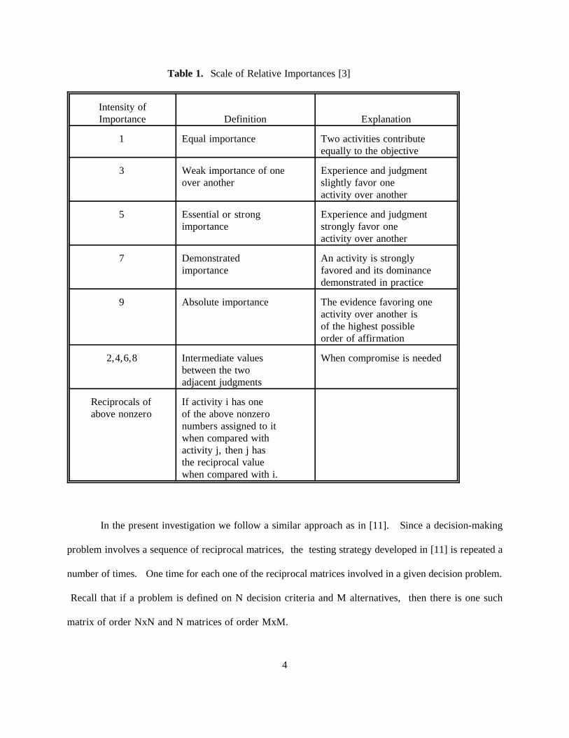
achieved by using the scale presented in table 1. That is not to say that a discrete set or even continuous

values could not be used, for it is known that even continuous values satisfy the Saaty axioms [27].

However, in practice the above discrete set is almost always used. After a decision maker forms the

entries of all the pertinent reciprocal matrices, an approach based on eigenvalue theory is used to derive

the relative weights of each criterion and also of each alternative in terms of each criterion in a

decision-making problem. An investigation on the development and performance of alternative scales for

quantifying pairwise comparisons can be found in [40].

Triantaphyllou and Mann in [11] tested the eigenvalue approach under a data continuity

assumption. According to this assumption the actual (and thus unknown) values of the pairwise

comparisons take on continuous values and not necessarily discrete ones. That continuity assumption is

made in order to capture the continuous nature of most real life decision-making problems. In that

investigation it was found that the eigenvalue approach is likely to yield a ranking of elements that is

different than the ranking yielded when actual data were used.

4

Table 1. Scale of Relative Importances [3]

Intensity ofImportance Definition Explanation

1 Equal importance Two activities contributeequally to the objective

3 Weak importance of oneover another

Experience and judgment slightly favor oneactivity over another

5 Essential or strongimportance

Experience and judgmentstrongly favor oneactivity over another

7 Demonstratedimportance

An activity is stronglyfavored and its dominancedemonstrated in practice

9 Absolute importance The evidence favoring oneactivity over another isof the highest possibleorder of affirmation

2,4,6,8 Intermediate valuesbetween the twoadjacent judgments

When compromise is needed

Reciprocals of above nonzero

If activity i has oneof the above nonzero numbers assigned to itwhen compared withactivity j, then j hasthe reciprocal valuewhen compared with i.

In the present investigation we follow a similar approach as in [11]. Since a decision-making

problem involves a sequence of reciprocal matrices, the testing strategy developed in [11] is repeated a

number of times. One time for each one of the reciprocal matrices involved in a given decision problem.

Recall that if a problem is defined on N decision criteria and M alternatives, then there is one such

matrix of order NxN and N matrices of order MxM.

5

In [11] it was found that when the eigenvalue method is used to derive relative weights, then it

is possible for some items (that is, decision criteria or alternatives) to have the same rank while in reality

they are distinct. However, the present paper demonstrates that it is possible alternatives which in reality

are less important than others to appear to be more important after the AHP or the revised AHP are

used. Furthermore, this problem of rank reversals is more severe in the present investigation. Also,

the present findings reveal that the rate of the rank reversals increases dramatically as the number of

alternatives increases.

In the following sections we briefly review the notion of the Saaty reciprocal, the eigenvalue

approach of deriving weights, the AHP method, the revised AHP method, as well as other relevant

concepts.

SOME BACKGROUND INFORMATION

Reciprocal Matrices with Pairwise Comparisons.

Let A1, A2,...,An be the members of a fuzzy set. This can be a set of alternatives which the

decision maker needs to evaluate in terms of a singe decision criterion. We are interested in evaluating

the membership values (i.e., the relative weights) of the above members. Saaty [1], [2], [3] proposes

to use a matrix A of rational numbers taken from the finite set: {1/9,1/8,...,1,2,...,8,9}. Each entry of

the above matrix A represents a pairwise judgment. Specifically, the entry aij denotes the number which

estimates the relative membership value of element Ai when it is compared with element Aj. Obviously,

aij = 1/aji and aii = 1. That is, the matrix A is a reciprocal one. Saaty in [3] asserts that the desired

relative membership values are the elements of the principle right eigenvector of matrix A. More

discussion on the problem of how to estimate relative membership values from such matrices can be found

in [10].

Saaty estimates the principal right eigenvector of the reciprocal matrices by multiplying the entries

6

in each row of matrix A together and then taking the n-th root (n is the number of the elements in the

fuzzy set). Since in the AHP it is desired to have values that add up to 1.00 the previously found vector

is normalized by dividing each entry by the sum of the above values. If we want (as is the case in the

revised AHP method) the element with the highest value to have membership value equal to 1.00, then

we need to divide the previously found vector by the highest value.

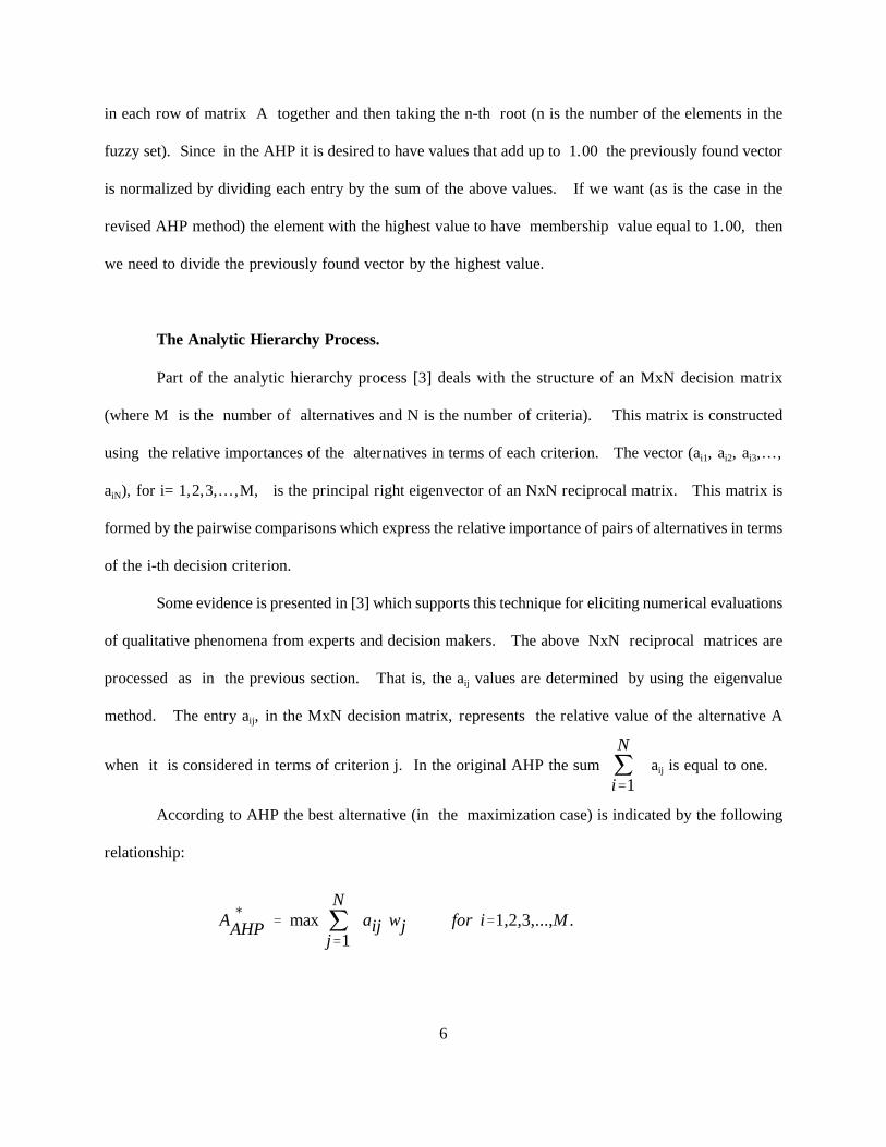
The Analytic Hierarchy Process.

Part of the analytic hierarchy process [3] deals with the structure of an MxN decision matrix

(where M is the number of alternatives and N is the number of criteria). This matrix is constructed

using the relative importances of the alternatives in terms of each criterion. The vector (ai1, ai2, ai3,...,

aiN), for i=1,2,3,...,M, is the principal right eigenvector of an NxN reciprocal matrix. This matrix is

formed by the pairwise comparisons which express the relative importance of pairs of alternatives in terms

of the i-th decision criterion.

Some evidence is presented in [3] which supports this technique for eliciting numerical evaluations

of qualitative phenomena from experts and decision makers. The above NxN reciprocal matrices are

processed as in the previous section. That is, the aij values are determined by using the eigenvalue

method. The entry aij, in the MxN decision matrix, represents the relative value of the alternative A

when it is considered in terms of criterion j. In the original AHP the sum aij is equal to one.jN

i'1

According to AHP the best alternative (in the maximization case) is indicated by the following

relationship:

A(

AHP ' max jN

j'1aij wj for i'1,2,3,...,M .

7

The Revised Analytic Hierarchy Process.

Belton and Gear [24] propose a revised version of the original AHP model. They demonstrate

that an inconsistency can occur when the AHP is used. A numerical example is presented in [24] which

consists of three decision criteria and three alternatives. The indication of the best alternative changes

when an alternative identical to one of the nonoptimal alternatives is introduced (thus creating four

alternatives). According to the authors the root for that inconsistency is the fact that the relative values

for each criterion sum up to one. Instead of having the relative values of the alternatives A1, A2, A3,...,

AM sum up to 1.00, they propose to divide each relative value in the columns of the decision matrix by

the maximum value of that column.

THE CONCEPTS OF THE RCP AND CDP MATRICES

The following forward error analysis is based on the assumption that in the real world the

membership values in a fuzzy set take on continuous values. This assumption is believed to be a

reasonable one since it captures the majority of real world cases. As it was mentioned earlier, these

members could be a set of alternatives to be examined in terms of a given decision criterion. In this case

the membership function expresses the degree that these alternatives meet the single decision criterion.

Let T1,T3,T3,..., Tn be the real (and thus unknown) membership values of a fuzzy set with

n members. If the decision maker knew the above real values, then he would be able to construct a

matrix with the real pairwise comparisons. In this matrix, say matrix A, the entries are "ij = Ti/ Tj. This

matrix is called the Real Continuous Pairwise matrix, or the RCP matrix. Since in the real world the

Ti's are unknown, so are the entries "ij of the previous matrix. However, we can assume here that the

decision maker instead of an unknown entry "ij is able to determine the closest values taken from the set:

{1/9,1/8,...,1,2,...,8,9}. That is, instead of the real (and thus unknown) value "ij one is able to

determine aij such that:

8

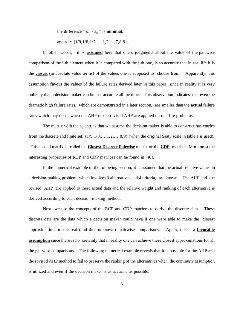
the difference * "ij - aij * is minimal,

and aij , {1/9,1/8,1/7,...,1,2,...,7,8,9}.

In other words, it is assumed here that one's judgments about the value of the pairwise

comparison of the i-th element when it is compared with the j-th one, is so accurate that in real life it is

the closest (in absolute value terms) of the values one is supposed to choose from. Apparently, this

assumption favors the values of the failure rates derived later in this paper, since in reality it is very

unlikely that a decision maker can be that accurate all the time. This observation indicates that even the

dramatic high failure rates, which are demonstrated in a later section, are smaller than the actual failure

rates which may occur when the AHP or the revised AHP are applied on real life problems.

The matrix with the aij entries that we assume the decision maker is able to construct has entries

from the discrete and finite set: {1/9,1/8,...,1,2,...,8,9} (when the original Saaty scale in table 1 is used).

This second matrix is called the Closest Discrete Pairwise matrix or the CDP matrix. More on some

interesting properties of RCP and CDP matrices can be found in [40].

In the numerical example of the following section, it is assumed that the actual relative values in

a decision-making problem, which involves 3 alternatives and 4 criteria, are known. The AHP and the

revised AHP are applied to these actual data and the relative weight and ranking of each alternative is

derived according to each decision-making method.

Next, we use the concepts of the RCP and CDP matrices to derive the discrete data. These

discrete data are the data which a decision maker could have if one were able to make the closest

approximations to the real (and thus unknown) pairwise comparisons. Again, this is a favorable

assumption since there is no certainty that in reality one can achieve these closest approximations for all

the pairwise comparisons. The following numerical example reveals that it is possible for the AHP and

the revised AHP method to fail to preserve the ranking of the alternatives when the continuity assumption

is utilized and even if the decision maker is as accurate as possible.

9

A NUMERICAL EXAMPLE

Suppose that a decision-making problem with 3 alternatives and 4 criteria has in reality the

following matrix as the decision matrix with the actual relative weights:

Criterion 1 2 3 4

Alt. (0.1325 0.0890 0.5251 0.2533) A1 0.5008 0.4804 0.0850 0.2113 A2 0.3785 0.2133 0.4434 0.3799 A3 0.1207 0.3063 0.4716 0.4089

That is, the actual relative weights of the 4 criteria are: (0.1325 0.0890 0.5251 0.2533). The

relative importances of the 3 alternatives in terms of the first criterion are: (0.5008 0.3785 0.1207), and

so on.

The above values can also be viewed as the principal right eigenvectors of the following 1 + 4

= 5 perfectly consistent RCP matrices. For the case of the four criteria we have:

RCP0 '

1 1.4890 0.2524 0.5231

0.6716 1 0.1695 0.3513

3.9622 5.8995 1 2.0727

1.9116 2.8462 0.4825 1

For instance, in the previous matrix the (1,2) entry is equal to 1.4890 because the corresponding pairwise

comparison is: 0.1325/0.0890 (= 1.4890). Similar interpretations hold for the remaining entries. For

the three alternatives we have in terms of each of the four criteria:

RCP1 '

1 1.3230 4.1502

0.7559 1 3.1371

0.2410 0.3188 1

RCP2 '

1 2.2552 1.5682

0.4440 1 0.6963

0.6377 1.4362 1

10

RCP3 '

1 0.1917 0.1803

5.2156 1 0.9403

5.5468 1.0635 1

RCP4 '

1 0.5561 0.5167

1.7982 1 0.9291

1.9355 1.0763 1

Applying the AHP and the revised AHP it can be shown that the following results are obtained:

The AHP solution The revised AHP solution

Alt. weights ranking weights ranking

A1 0.2073 3 0.2048 3

A2 0.3982 1 0.3980 1

A3 0.3945 2 0.3972 2

In reality, however, the decision maker does not know the previous real values. Instead, one has

to use matrices with entries from the set: {1/9,1/8,...,1,2,...,8,9} (that is, to use the scale presented in

table 1). The CDP matrices which best approximate the previous 5 RCP matrices can be shown to be as

follows. For the case of the four criteria the corresponding CDP matrix and its corresponding eigenvector

is:

RCP0 6 CDP0 '

1 1.5000 0.2500 0.5000

0.6667 1 0.1667 0.3333

4.0000 6.0000 1 2.0000

2.0000 3.0000 0.5000 1

6

0.1304

0.0870

0.5217

0.2609

For instance, the (1,2) entry in the previous matrix is equal to 1.5000 because the corresponding entry in

the RCP matrix is 1.4890 and the value 1.5000 is the closest value from the permissible values (when the

scale in table 1 is used). Similar interpretations hold for the remaining entries.

Similarly with above, for the three alternatives in terms of each one of the four criteria the CDP

matrices and their corresponding eigenvectors are:

11

RCP1 6 CDP1 '

1 1.3333 4.0000

0.7500 1 3.0000

0.2500 0.3333 1

6

0.5000

0.3750

0.1250

RCP2 6 CDP2 '

1 2.2500 1.6000

0.4444 1 0.7143

0.6250 1.4000 1

6

0.4833

0.2151

0.3016

RCP3 6 CDP3 '

1 0.2000 0.1667

5.0000 1 0.8889

6.0000 1.1250 1

6

0.0835

0.4264

0.4901

RCP4 6 CDP4 '

1 0.5556 0.5000

1.8000 1 0.8889

2.0000 1.1250 1

6

0.2083

0.3734

0.4183

That is, the data which are assumed to be available in reality to the decision maker for the

present problem are:

Criterion 1 2 3 4 Alt. (0.1304 0.0870 0.5217 0.2609) A1 0.5000 0.4833 0.0835 0.2083 A2 0.3750 0.2151 0.4264 0.3734 A3 0.1250 0.3016 0.4901 0.4183

Similarly, as in the first part of this example, the AHP and the revised AHP yield the following results:

12

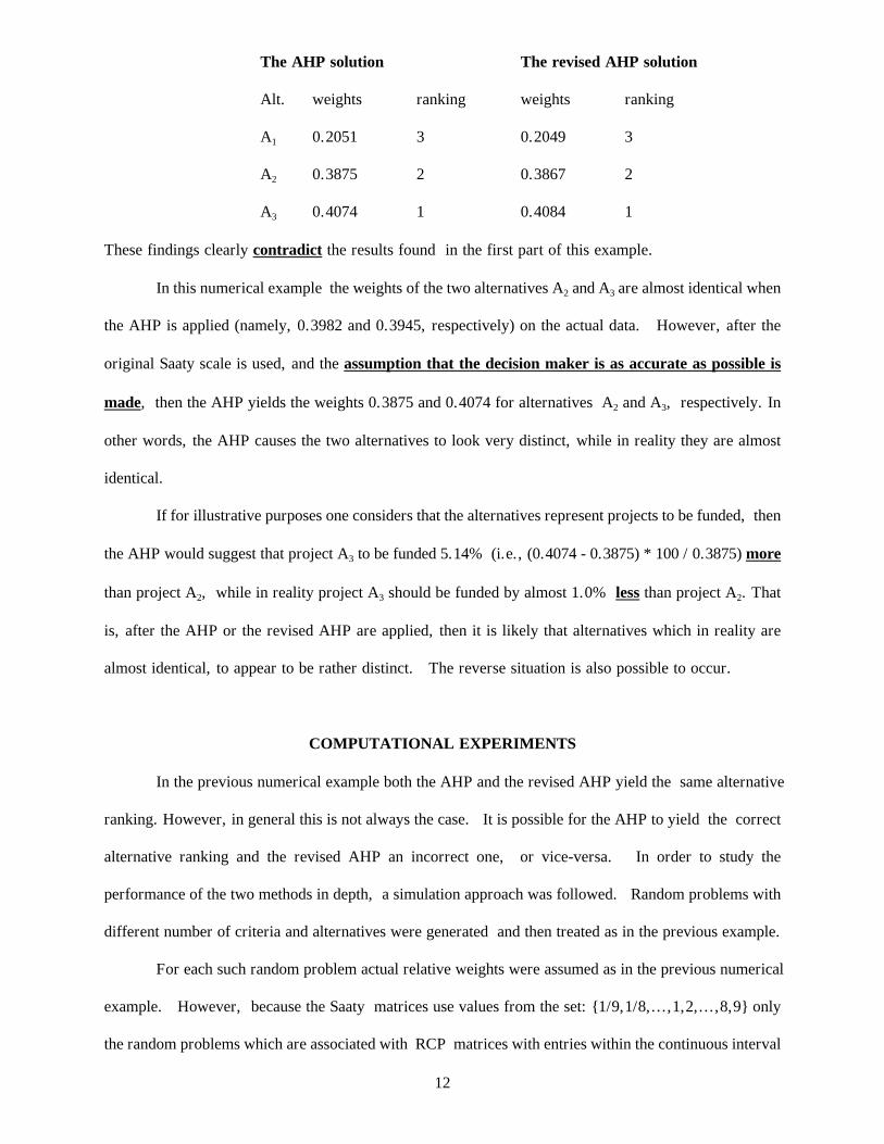
The AHP solution The revised AHP solution

Alt. weights ranking weights ranking

A1 0.2051 3 0.2049 3

A2 0.3875 2 0.3867 2

A3 0.4074 1 0.4084 1

These findings clearly contradict the results found in the first part of this example.

In this numerical example the weights of the two alternatives A2 and A3 are almost identical when

the AHP is applied (namely, 0.3982 and 0.3945, respectively) on the actual data. However, after the

original Saaty scale is used, and the assumption that the decision maker is as accurate as possible is

made, then the AHP yields the weights 0.3875 and 0.4074 for alternatives A2 and A3, respectively. In

other words, the AHP causes the two alternatives to look very distinct, while in reality they are almost

identical.

If for illustrative purposes one considers that the alternatives represent projects to be funded, then

the AHP would suggest that project A3 to be funded 5.14% (i.e., (0.4074 - 0.3875) * 100 / 0.3875) more

than project A2, while in reality project A3 should be funded by almost 1.0% less than project A2. That

is, after the AHP or the revised AHP are applied, then it is likely that alternatives which in reality are

almost identical, to appear to be rather distinct. The reverse situation is also possible to occur.

COMPUTATIONAL EXPERIMENTS

In the previous numerical example both the AHP and the revised AHP yield the same alternative

ranking. However, in general this is not always the case. It is possible for the AHP to yield the correct

alternative ranking and the revised AHP an incorrect one, or vice-versa. In order to study the

performance of the two methods in depth, a simulation approach was followed. Random problems with

different number of criteria and alternatives were generated and then treated as in the previous example.

For each such random problem actual relative weights were assumed as in the previous numerical

example. However, because the Saaty matrices use values from the set: {1/9,1/8,...,1,2,...,8,9} only

the random problems which are associated with RCP matrices with entries within the continuous interval

13

[1/9, 9/1] were considered. Each test problem was treated as in the previous example. If the AHP or

the revised AHP yielded a ranking different than the one derived when actual data were used, then the

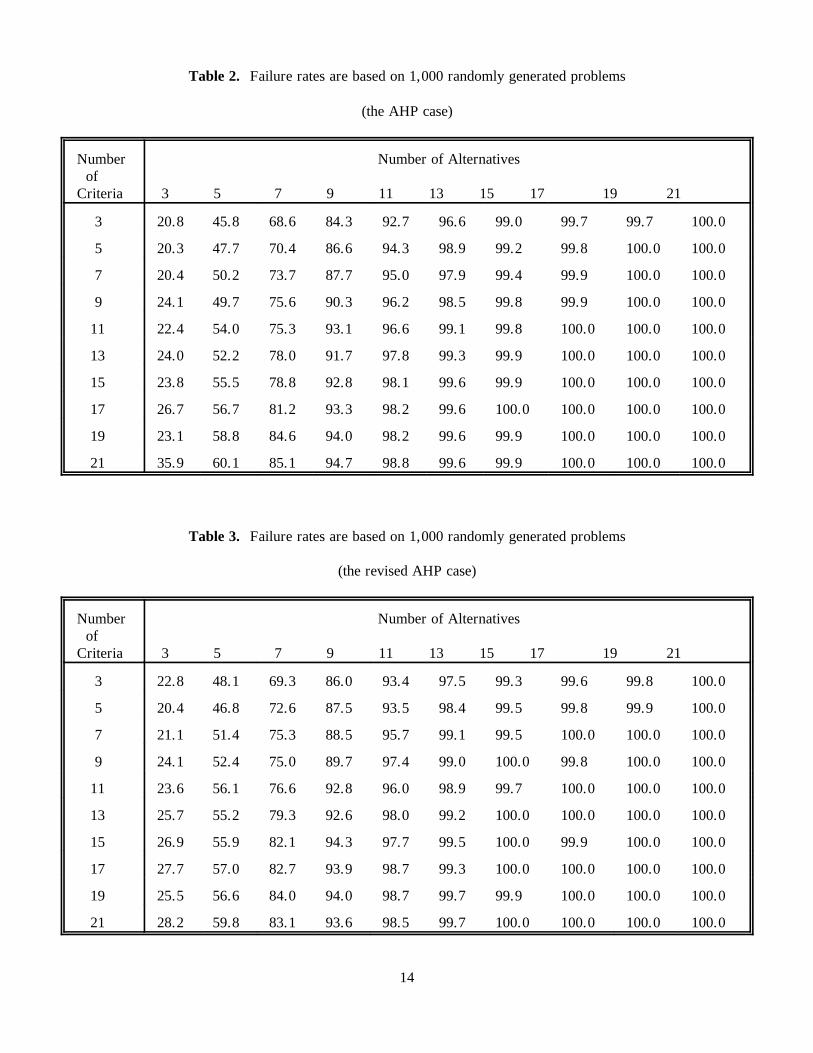
case was recorded as a failure. Tables 2 and 3 present the results of this simulation approach for random

problems of different sizes. Table 2 deals with the AHP and table 3 with the revised AHP. Figures

1 and 2 graphically depict the results presented in tables 2 and 3, respectively. The simulation

program was written in FORTRAN and the random numbers were generated by using the IMSL library

of subroutines.

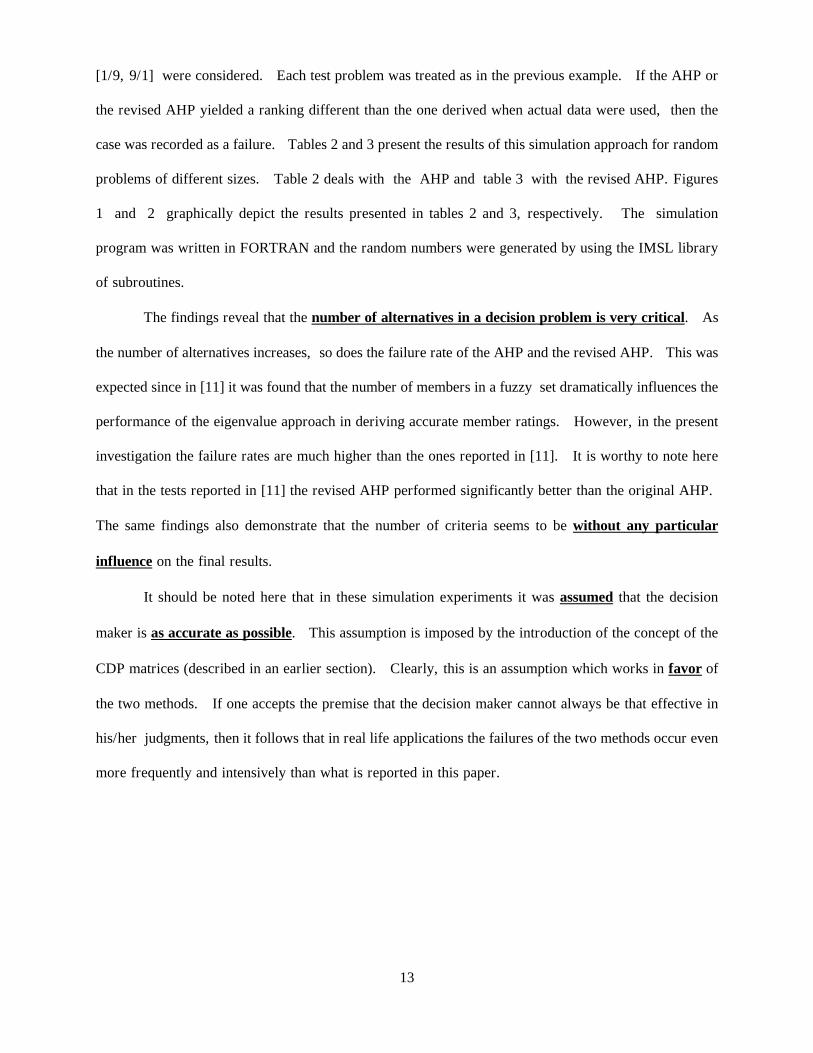
The findings reveal that the number of alternatives in a decision problem is very critical. As

the number of alternatives increases, so does the failure rate of the AHP and the revised AHP. This was

expected since in [11] it was found that the number of members in a fuzzy set dramatically influences the

performance of the eigenvalue approach in deriving accurate member ratings. However, in the present

investigation the failure rates are much higher than the ones reported in [11]. It is worthy to note here

that in the tests reported in [11] the revised AHP performed significantly better than the original AHP.

The same findings also demonstrate that the number of criteria seems to be without any particular

influence on the final results.

It should be noted here that in these simulation experiments it was assumed that the decision

maker is as accurate as possible. This assumption is imposed by the introduction of the concept of the

CDP matrices (described in an earlier section). Clearly, this is an assumption which works in favor of

the two methods. If one accepts the premise that the decision maker cannot always be that effective in

his/her judgments, then it follows that in real life applications the failures of the two methods occur even

more frequently and intensively than what is reported in this paper.

14

Table 2. Failure rates are based on 1,000 randomly generated problems

(the AHP case)

Number of Criteria

Number of Alternatives

3 5 7 9 11 13 15 17 19 21

3 20.8 45.8 68.6 84.3 92.7 96.6 99.0 99.7 99.7 100.0

5 20.3 47.7 70.4 86.6 94.3 98.9 99.2 99.8 100.0 100.0

7 20.4 50.2 73.7 87.7 95.0 97.9 99.4 99.9 100.0 100.0

9 24.1 49.7 75.6 90.3 96.2 98.5 99.8 99.9 100.0 100.0

11 22.4 54.0 75.3 93.1 96.6 99.1 99.8 100.0 100.0 100.0

13 24.0 52.2 78.0 91.7 97.8 99.3 99.9 100.0 100.0 100.0

15 23.8 55.5 78.8 92.8 98.1 99.6 99.9 100.0 100.0 100.0

17 26.7 56.7 81.2 93.3 98.2 99.6 100.0 100.0 100.0 100.0

19 23.1 58.8 84.6 94.0 98.2 99.6 99.9 100.0 100.0 100.0

21 35.9 60.1 85.1 94.7 98.8 99.6 99.9 100.0 100.0 100.0

Table 3. Failure rates are based on 1,000 randomly generated problems

(the revised AHP case)

Number of Criteria

Number of Alternatives

3 5 7 9 11 13 15 17 19 21

3 22.8 48.1 69.3 86.0 93.4 97.5 99.3 99.6 99.8 100.0

5 20.4 46.8 72.6 87.5 93.5 98.4 99.5 99.8 99.9 100.0

7 21.1 51.4 75.3 88.5 95.7 99.1 99.5 100.0 100.0 100.0

9 24.1 52.4 75.0 89.7 97.4 99.0 100.0 99.8 100.0 100.0

11 23.6 56.1 76.6 92.8 96.0 98.9 99.7 100.0 100.0 100.0

13 25.7 55.2 79.3 92.6 98.0 99.2 100.0 100.0 100.0 100.0

15 26.9 55.9 82.1 94.3 97.7 99.5 100.0 99.9 100.0 100.0

17 27.7 57.0 82.7 93.9 98.7 99.3 100.0 100.0 100.0 100.0

19 25.5 56.6 84.0 94.0 98.7 99.7 99.9 100.0 100.0 100.0

21 28.2 59.8 83.1 93.6 98.5 99.7 100.0 100.0 100.0 100.0

15

Fig. 1. Failure rates are based on 1,000 randomly generated problems(the AHP case)

Fig. 2. Failure rates are based on 1,000 randomly generated problems(the revised AHP case)

16

From the above observations it is concluded that if one uses the AHP or the revised AHP in order to select the

best alternative, then he/she may instead select an alternative which is not the best. Similarly, if one is interested in

determining the relative weights of the alternatives, then distortions in the calculated weights are possible.

The answer to the critical question whether the numerical anomalies reported here are severe or not, depends on

the particular application under consideration, and no generalizations can be made. If the impact of choosing a non-

optimal alternative is not that severe, then the decision maker should not be highly concerned. However, if the application

is very critical, then the present investigation may serve as a warning for caution before reaching the final decision. The

present investigation reaffirms the belief of many practitioners today, that multi-attribute decision-making methods should

be used only as decision support tools, and not to be taken literally.

CONCLUDING REMARKS

In this paper we investigated the reversals in the alternative ranking which occur when Saaty pairwise comparison

matrices are used as input in decision-making problems. Saaty pairwise comparison matrices are widely considered as

successful means for gathering data in many real world decision-making situations. The AHP and some of its variants

have found a considerable appeal in approaching many real life engineering applications. Many computer packages have

been developed (see, for instance, [13]) to automate their application to real life problems.

The forward error analysis in this paper reveals that when the AHP or the revised AHP methods are used in

combination with the eigenvalue approach for processing the input data, then severe alternative ranking failures are

possible. These failures are more dramatic as the number of alternatives increases. However, even for decision problems

with a few alternatives the possibility of ranking alterations is significantly high. The number of criteria or the

decision-making method used (i.e., the AHP or the revised AHP) seem to be without any particular influence in the above

rates. Therefore, these results can be used to properly guide the decision maker when applying these methods to real life

engineering problems.

The present paper provides a justification on why the application of the AHP (or the revised AHP) should be

treated with some skepticism and their results not to be taken literally. This consideration comes in symphony with the

concerns expressed by other researchers in the past (see, for instance, [24], [29], [25], [26], [30], and [33]). However,

17

the assumption that the decision maker is as accurate as possible in deriving his/her judgments (i.e., the concept of the

CDP matrices ) and its application in evaluating multi-criteria decision making methods is a very new one.

It is worthy to emphasize here that in under less than perfect conditions the real failure rates can be even more

dramatic. It should also be kept in mind, that the present investigation is based on the assumption that the actual data

for evaluating alternatives in terms of decision criteria, take on continuous values. Therefore, the previous results are

subject to this continuity assumption.

The present results, along with the realization that data in multi-attribute decision-making problems are constant,

urge for the need to perform a sensitivity analysis on any real life decision problem. Masuda in [41] presents a very

interesting approach for performing a sensitivity analysis when the AHP is used. Another approach for performing a

systematic sensitivity analysis when the AHP is used, is due to Sanchez and Triantaphyllou [42]. Note that the computer

software EXPERT CHOICE, which is based on the AHP, also allows for some preliminary sensitivity analysis. It is

highly advised that a sensitivity analysis should be always be applied in real applications, especially when some alternatives

appear to be close to each other.

Finally, it should be stated here that the same investigation, besides being a mechanism for testing future models,

also reveals that there is an open problem in this class of decision-making models and more research in this topic is

needed.

REFERENCES

1. T.L. Saaty. A Scaling Method for Priorities in Hierarchical Structures. Journal of Mathematical Psychology,

15, 57-68 (1977).

2. T.L. Saaty. Exploring the interface between hierarchies, multiple objects and fuzzy sets, Journal of Fuzzy Sets

and Systems, 1, 57-68 (1978).

3. T.L. Saaty. The Analytic Hierarchy Process, McGraw-Hill International, New York, NY (1980).

4. A.T.W. Chu, R.E. Kalaba, and K. Spingarn. A Comparison of Two Methods for Determining the Weights of

Belonging to Fuzzy Sets. Journal of Optimization Theory and Applications, 27, 531-538 (1979).

18

5. V.V. Federov, V.B. Kuz'min, V.B., and A.I. Vereskov. Membership Degrees Determination from Saaty Matrix

Totalities, Institute for System Studies, Moscow, USSR. Paper appeared in: Approximate Reasoning in Decision

Analysis, M.M. Gupta, and E. Sanchez (editors), North-Holland Publishing Company, 23-30 (1982).

6. J.I. Khurgin, and V.V. Polyakov. Fuzzy Analysis of the Group Concordance of Expert Preferences, defined by

Saaty Matrices. Fuzzy Sets Applications, Methodological Approaches and Results, Akademie-Verlag Berlin,

111-115 (1986).

7. J.I. Khurgin, and V.V. Polyakov (1986). Fuzzy Approach to the Analysis of Expert Data. Fuzzy Sets

Applications, Methodological Approaches and Results, Akademie-Verlag Berlin, 116-124 (1986).

8. E. Triantaphyllou and S.H. Mann. An Examination of the Effectiveness of Multi-Dimensional Decision-Making

Methods: A Decision-Making Paradox, International Journal of Decision Support Systems, 5, 303-312 (1989).

9. E. Triantaphyllou, P.M. Pardalos, and S.H. Mann. A Minimization Approach to Membership Evaluation in

Fuzzy Sets and Error Analysis, Journal of Optimization Theory and Applications, 66(2), 275-287 (1990).

10. E. Triantaphyllou, P.M. Pardalos, and S.H. Mann. The Problem of Evaluating Membership Values in Real

World Situations. Operations Research and Artificial Intelligence: The Integration of Problem Solving Strategies,

(D.E. Brown and C.C. White III, editors), Kluwer Academic Publishers, 197-214 (1990).

11. E. Triantaphyllou and S.H. Mann. An Evaluation of the Eigenvalue Approach for Determining the Membership

Values in Fuzzy Sets. Fuzzy Sets and Systems. 35(3), 295-301 (1990).

12. L.G. Vargas. Reciprocal Matrices with Random Coefficients. Mathematical Modeling, 3, 69-81 (1982).

13. Decision Support Software, Inc. Expert Choice Software Package. McLean, Virginia (1986).

14. R. Putrus. Accounting for Intangibles in Integrated Manufacturing (nonfinancial justification based on the

Analytical Hierarchy Process). Information Strategy, 6, 25-30 (1990).

15. C. Falkner and S. Benhajla. Multi-attribute Decision Models in the Justification of CIM Systems. The

Engineering Economist, 35, 91-114 (1990).

16. K. Swann and W.D. O'Keefe. Advanced Manufacturing Technology: Investment Decision Process.

Management Decisions, 28(1), 20-31 (1990).

19

17. G.C. Roper-Lowe and J.A. Sharp. The Analytic Hierarchy Process and its Application to an Information

Technology Decision. Operational Research Society Ltd., 41(1), 49-59 (1990).

18. J. Finnie. The Role of Financial Appraisal in Decisions to Acquire Advanced Manufacturing Technology.

Accounting and Business Research, 18(7), 133-139 (1988).

19. T.O. Boucher and E.L. McStravic. Multi-attribute Evaluation within a Present Value Framework and its Relation

to the Analytic Hierarchy Process. The Engineering Economist, 37(1), 55-71 (1991).

20. R.N. Wabalickis. Justification of FMS with the Analytic Hierarchy Process. Journal of Manufacturing Systems,

17(3), 175-182 (1988).

21. K.E. Cambron and G.W. Evans. Layout Design Using the Analytic Hierarchy Process. Computers & IE. 20(2)

221-229 (1991).

22. L. Wang and T. Raz. Analytic Hierarchy Process Based on Data Flow Problem. Computers & IE. 20(3) 355-

365 (1991).

23. A. Arbel and A. Seidmann. Selecting a Microcomputer for Process Control and Data Acquisition. IEE Trans.

16(1) (1984).

24. V. Belton and T. Gear. On a Short-coming of Saaty's Method of Analytic Hierarchies. Omega, 228-230 (1983).

25. J.S. Dyer and H.V. Ravinder. Irrelevant Alternatives and the Analytic Hierarchy Process. Working Paper,

Department of Management, The University of Texas at Austin, (1983).

26. J.S. Dyer and R.E. Wendell. A Critique of the Analytic Hierarchy Process. Working Paper 84/85-4-24,

Department of Management, The University of Texas at Austin, (1985).

27. T.L. Saaty. Axiomatic Foundations of the Analytic Hierarchy Process. Management Science, 32(7), 841-855

(1983).

28. T.L. Saaty. Rank Generation, Preservation, and Reversal in the Analytic Hierarchy Process. Decision Sciences,

18, 157-177 (1987).

29. J.S. Dyer. Remarks on the Analytic Hierarchy Process. Management Science, 36(3), 249-258 (1990).

30. J.S. Dyer. A Clarification of "Remarks on the Analytic Hierarchy Process". Management Science, 36(3),

20

274-275 (1990).

31. T.L. Saaty. An Exposition of the AHP in Reply to the Paper "Remarks on the Analytic Hierarchy Process".

Management Science, 36(3), 259-268 (1990).

32. P.T. Harker and L.G. Vargas. Reply to "Remarks on the Analytic Hierarchy Process". Management Science,

36(3), 269-273 (1990).

33. R.L. Winkler. Decision Modeling and Rational Choice: AHP and Utility Theory. Management Science, 36(3),

247-248 (1990).

34. D.E. Bell and P.H. Farquhar. Perspectives on Utility Theory. Operations Research, 34, 179-183 (1986).

35. R.M. Hogarth and M.W. Reder, (Eds.). Rational Choice: The Contrast Between Economics and Psychology,

University of Chicago Press, Chicago, Illinois, (1986).

36. M. Weber and C. Camerer. Recent Developments in Modeling Preferences Under Risk. OR Spectrum, 9,

129-151 (1987).

37. B.R. Munier (Ed.). Risk, Decision and Rationality. D. Reidel, Dordrecht, Holland, 1988.

38. P.C. Fishburn and I.H. LaValle (Eds.). Annals of Operations Research. Volume 19: Choice Under Uncertainty.

J.C. Baltzer, Basel, Switzerland, 1989.

39. R.K. Sarin. Analytical Issues in Decision Methodology. In I. Horowitz (Ed.), Organization and Decision Theory,

Kluwer- Nijhoff, Dordrecht, Holland, 156-172 (1989).

40. E. Triantaphyllou, F.A. Lootsma, P.M. Pardalos, and S.H. Mann. On the Evaluation and Application of

Different Scales For Quantifying Pairwise Comparisons in Fuzzy Sets. Multi-Criteria Decision Analysis, 3(3),

133-155 (1993).

41. T. Masuda. Hierarchical Sensitivity Analysis of the Priorities Used in the Analytic Hierarchy Process. Int. J.

of Systems Science, 21(2), 415-427 (1990).

42. E. Triantaphyllou and A. Sanchez and E. Triantaphyllou. A Sensitivity Analysis Approach for Some

Deterministic Multi-Criteria Decision-Making. Decision Sciences, 28(1), 151-194 (1997).