A Dynamic Flight Model for Slocum Gliders and Implications for TurbulenceMicrostructure Measurements

LUCAS MERCKELBACH AND ANJA BERGER

Institute of Coastal Research, Helmholtz-Zentrum Geesthacht, Geesthacht, Germany

GERD KRAHMANN AND MARCUS DENGLER

GEOMAR Helmholtz Centre for Ocean Research Kiel, Kiel, Germany

JEFFREY R. CARPENTER

Institute of Coastal Research, Helmholtz-Zentrum Geesthacht, Geesthacht, Germany

(Manuscript received 20 September 2018, in final form 14 December 2018)

ABSTRACT

The turbulent dissipation rate « is a key parameter tomany oceanographic processes. Recently, gliders have

been increasingly used as a carrier formicrostructure sensors. Compared to conventional ship-basedmethods,

glider-based microstructure observations allow for long-duration measurements under adverse weather

conditions and at lower costs. The incident water velocity U is an input parameter for the calculation of the

dissipation rate. SinceU cannot bemeasured using the standard glider sensor setup, the parameter is normally

computed from a steady-state glider flight model. As « scales with U2 or U4, depending on whether it is

computed from temperature or shear microstructure, respectively, flight model errors can introduce a sig-

nificant bias. This study is the first to use measurements of in situ glider flight, obtained with a profiling

Doppler velocity log and an electromagnetic current meter, to test and calibrate a flight model, extended to

include inertial terms. Compared to a previously suggested flight model, the calibrated model removes a bias

of approximately 1 cm s21 in the incident water velocity, which translates to roughly a factor of 1.2 in estimates

of the dissipation rate. The results further indicate that 90% of the estimates of the dissipation rate from the

calibratedmodel are within a factor of 1.1 and 1.2 formeasurements derived frommicrostructure temperature

sensors and shear probes, respectively. We further outline the range of applicability of the flight model.

1. Introduction

The dissipation rate of turbulent kinetic energy is a

parameter that plays a key role in many physical and

biogeochemical processes in oceans and coastal seas.

However, direct oceanic measurements of turbulence

are relatively scarce, as most observations stem from

free-falling profilers, operated from seagoing vessels.

The monetary and labor cost of taking such profiles is

therefore substantial, and is most often limited to rela-

tively calm conditions.

An emerging alternative to ship-based profiling is the

use of ocean gliders, a class of buoyancy-driven auton-

omous underwater vehicles (Griffiths 2002, chapter 3;

Rudnick 2016). Although gliders have been increasingly

used over almost two decades, it is only recently that

turbulence profilers have been mounted onto gliders

(Wolk et al. 2009; Fer et al. 2014; Peterson and Fer 2014;

Palmer et al. 2015; Schultze et al. 2017; St. Laurent and

Merrifield 2017; Scheifele et al. 2018). The glider as a

measurement platform has relatively low levels of

vibration and mechanical noise, mainly because of the

absence of a propeller. This makes gliders suitable for

turbulence observations using shear probes. Using gliders

as an alternative to oceangoing ships removes a sub-

stantial part of the human factor in the data collection

process and therefore eases long-duration data collec-

tion while reducing costs, and it effectively removes any

measurement constraints imposed by adverse weather

conditions.

Despite the advantages of glider-based turbulence

measurements, the major drawback of this setup is the

uncertainty in the flight of the glider.A required parameterCorresponding author: Lucas Merckelbach, lucas.merckelbach@

hzg.de

FEBRUARY 2019 MERCKELBACH ET AL . 281

DOI: 10.1175/JTECH-D-18-0168.1

� 2019 American Meteorological Society. For information regarding reuse of this content and general copyright information, consult the AMS CopyrightPolicy (www.ametsoc.org/PUBSReuseLicenses).

Unauthenticated | Downloaded 04/04/22 11:50 PM UTC

in the processing of microstructure shear and temperature

measurements is the speed of flow past the sensors. The

speed through water enters the processing raised to the

fourth power when using airfoil shear probes, and to

the second power when using microtemperature sen-

sors (see section 6a for details). For free-falling vertical

profilers, this is usually determined from the rate of

change of pressure. For glider-based measurements,

this gives only the vertical speed of the glider, with a

horizontal speed that must be either measured directly

or modeled.

It is uncommon for a microstructure glider to be

equipped with a device that directly measures (a hori-

zontal component of) the speed through water, so

often a flight model is used for the computation of

turbulent dissipation (Fer et al. 2014; Peterson and Fer

2014; Palmer et al. 2015; Schultze et al. 2017; St.

Laurent and Merrifield 2017; Scheifele et al. 2018).

The most commonly used flight model is that of

Merckelbach et al. (2010), who assume a steady-state

balance between buoyancy, drag, and lift, and use the

measured pitch angle and buoyancy change achieved

by the buoyancy engine to compute the speed through

water (Fer et al. 2014; Peterson and Fer 2014; Palmer

et al. 2015; Schultze et al. 2017; Scheifele et al. 2018).

The numerical evaluation of these forces requires

values to be attributed to a number of coefficients,

such as the glider density, compressibility, drag, and lift

coefficients. Merckelbach et al. (2010) show that the

glider density, compressibility, and drag coefficients

can be determined from standard glider sensors; how-

ever, they note that it is not possible to simulta-

neously determine the lift coefficient without a direct

measurement of the horizontal component of the glider

speed.1 The model therefore relies on tabulated co-

efficients from aerodynamic studies of bodies of similar

shape in its specification of lift coefficients. To date, no

study has been published where the glider flight model

by Merckelbach et al. (2010) is calibrated and com-

pared with direct measurements of the glider velocity

through water.

In summary, glider-based turbulence microstructure

measurements represent new possibilities for sampling

ocean turbulence, but they suffer from uncertainties in

glider flight models, which are particularly sensitive,

and as yet untested. In this work a Teledyne Webb

Research Slocum Electric Shallow glider has been

fitted with a Teledyne RD Instruments (RDI) Explorer

Doppler velocity log (DVL). This device primarily

measures the horizontal and vertical components of the

glider velocity with respect to the seabed (bottom

track), provided the seabed is within the acoustic range

of about 80m. A profiling mode also allows the mea-

surement of the glider velocity relative to the water at

some distance below the glider (about 5–15m). In ad-

dition, we also utilize data collected from an electro-

magnetic current meter mounted inside a microstructure

package to assess glider flight characteristics. Using

these data we calibrate and extend the glider flight

model of Merckelbach et al. (2010) based on direct

measurements of glider flight, as well as examine the

implications for the accuracy of turbulent dissipa-

tion rate estimates as measured with glider-mounted

microstructure sensors.

2. Background: Steady-state glider flight model

Key to the work presented herein is a steady-state

planar glider flight model developed by Merckelbach

et al. (2010) in order to obtain vertical water velocities

from glider observations. The model is based on a hor-

izontal (x) and vertical (z) force balance, in which the

acceleration terms are neglected, given by 2

05 sin(u1a)FL2 cos(u1a)F

D(1)

05FB2F

g2 cos(u1a)F

L2 sin(u1a)F

D, (2)

where the pitch angle u and the angle of attack a are

defined in Fig. 1. The forces that act on the glider are due

to buoyancy FB, gravity Fg, lift FL, and drag FD:

Fg5m

gg , (3)

FB5 grfV

g[12 «

cP1a

T(T2T

0)]1DV

bpg , (4)

FD51

2rSU2ðC

D01a2C

D1Þ , (5)

FL5

1

2rSU2C

L(a) , (6)

CL(a)5 aa , (7)

where mg is the mass of the glider, g is the acceleration

due to gravity, r is the in situ density,Vg is the volume of

the glider at atmospheric pressure, «c is the coefficient of

1Depth-averaged velocities computed using surface GPS data,

as attempted by Merckelbach et al. (2010), would provide such a

measurement. However, for calibrating the lift coefficient, water

velocities along the track of the glider must be known with a bias of

less than approximately 1 cm s21, making this method unreliable.

2 This system of equations is identical to the equations given by

Merckelbach et al. (2010), if their equations are corrected for an

unfortunate sign error.

282 JOURNAL OF ATMOSPHER IC AND OCEAN IC TECHNOLOGY VOLUME 36

Unauthenticated | Downloaded 04/04/22 11:50 PM UTC

compressibility, aT is the thermal expansion co-

efficient of the glider, DVbp is the volume change

achieved by the buoyancy engine, S is the total surface

area of the wings, U is the magnitude of the glider

speed through water, and CD0and CD1

are the parasite

and induced drag coefficients, respectively. For small

a, the lift coefficient CL is assumed to be linear in the

angle of attack, proportional to the lift angle co-

efficient a.

An expression for U can be obtained by either elimi-

nating FD or FL from (1) and (2), and substituting from

(5) and (6), respectively, relating U to either drag co-

efficients or lift angle coefficients. Expressed in drag

coefficients, we get

sin(u1a)(FB2F

g)2

1

2rSU2ðC

D01C

D1a2Þ5 0: (8)

In addition, an expression for the angle of attack is found

by combining (1), and (5)–(7), yielding

a5C

D01a2C

D1

atan(u1a). (9)

Equations (8) and (9) provide a model to compute the

steady-state flight condition at any time, given mea-

surements of the buoyancy drive, pitch angle, and in situ

density, and a set of model coefficients for drag, lift,

compressibility, and thermal expansion (if applicable).

Merckelbach et al. (2010) determine model coeffi-

cients by minimizing a cost function that is mathemati-

cally identical to

R05

1

N�N21

i50

�U[i] sin(u[i]1a[i])1

dh

dt[i]

�2

. (10)

Herein, the depth rate dh/dt and pitch u are observations

with index i from a total ofN values, andU and a are the

corresponding model results using (8) and (9), respec-

tively. It can be shown, however, that the cost function

does not yield unique values if both the parasite drag

and the lift angle coefficient are present in the minimi-

zation parameter space. Although the model may be

optimized for the vertical velocity component, the hor-

izontal velocity component, and therefore the speed

through water, depends on the actual value of the lift

angle coefficient. This means that depth-rate observa-

tions alone are not sufficient to calibrate a glider flight

model that also computes accurately the glider speed

through water. Consequently, additional measurements

of a nonvertical glider velocity component are required

and are presented in section 4.

3. Dynamic glider flight model

Although the steady-state glider flight assumption

seems reasonable for most practical situations, a dy-

namic nonsteady-state glider flight model may provide a

better estimate of the glider speed for rapidly chang-

ing conditions, for example, when strong density

gradients are present or around dive-to-climb turning

points. Requiring little additional effort, such a dy-

namic flight model can be obtained by (re)inserting

the acceleration terms into the steady-state model.

Besides the glider mass accounting for its inertia, the

so-called added mass needs to be considered. Added

mass terms arise from the fact that if a submerged

body accelerates, not only does the body’s mass op-

pose the acceleration, but also the flow around the

body changes. From an energy principle, it then fol-

lows that the body does work on the ambient water

mass and additional forces act on the submerged body

(Imlay 1961). These additional forces can be conve-

niently written as a 6 3 6 mass matrix, multiplied by a

vector composed of three linear and three angular

acceleration components (Newman 1977).

For planar flight with negligible rotational accelera-

tions, which are typical for glider flight, the inertial

forces to be inserted into the dimensional steady-state

model can be simplified to M[du/dt dw/dt]T. Herein u

and w are the horizontal and vertical glider velocity com-

ponents in a georeferenced coordinate system, respec-

tively; andM is a 23 2matrix, composed of the glidermass

on the diagonal, mgI, where I is the identity matrix, and a

23 2 matrixm, representing the addedmass terms.When

expressed in the orthogonal glider referenced coordinate

FIG. 1. Schematic representation of a glider, defining an or-

thogonal coordinate system with x and z axes, and an orthogonal

glider referenced coordinate system (j, h). The latter originates

from the former after a rotation of the pitch angle. The glider path

(dashed line)makes a small angle, equal to the angle of attack, with

the glider’s principal axis, which coincides with the j axis. The

forces resulting drag, lift, and net buoyancy are drawn by the yellow

vectors. The positions of the EMC sensor and the DVL are in blue

and red, respectively. The DVL is mounted such that the principal

axis of the DVL (dashed) makes an 118 angle with the h axis.

FEBRUARY 2019 MERCKELBACH ET AL . 283

Unauthenticated | Downloaded 04/04/22 11:50 PM UTC

system, (j, h) (see Fig. 1), with its axes (from the glider’s

perspective) pointing forward and upward, the added m

for a glider-shaped object can adequately be described by a

diagonal matrix, diag(m11, m22), where m11 and m22 are

the dominant added mass components (Imlay 1961;

Newman 1977). Expressed in the (x, y) coordinate system,

the transformed m is not necessarily diagonal, and the

inertia matrix becomes

M5mgI1

"m

11cos2(u)1m

22sin2(u) (m

112m

22) cos(u) sin(u)

(m112m

22) cos(u) sin(u) m

g1m

22cos2(u)1m

11sin2(u)

#. (11)

Based on the expressions given in Imlay (1961) for a

finned prolate spheroid–shaped glider with a length of

2 m, the numerical values of the added mass terms are

estimated at m11 5 0:2mg and m22 5 0:92mg.

With this result the dynamic flight model can be

written as [see (1), (2)]

Md

dt

�u

w

�5

"sin(u1a)F

L2 cos(u1a)F

D

FB2F

g2 cos(u1a)F

L2 sin(u1a)F

D

#.

(12)

To integrate this initial value problem using a classi-

cal Runge–Kutta (RK4) explicit method, we specify

u5w5 0 as initial conditions and when the glider is at

the surface. Furthermore, the incident flow velocity is set

equal to U5ffiffiffiffiffiffiffiffiffiffiffiffiffiffiffiffiu2 1w2

p. In fact, this is true only if the

water column behaves as a steady-state flow without

shear. However, under most conditions the oceanic shear

is small so that the errors of the estimated lift and drag

forces can be assumed small too. We also note that

transient effects caused by changing flow conditions on

the drag and lift forces generated are not accounted for.

Both the steady-state and dynamic models are im-

plemented in Python 3. The source code, documentation,

and examples are available at a public repository under

the MIT software license (Merckelbach 2018a,b).

4. Experimental data

a. Instrumentation

The glider COMET is a Teledyne Webb Research G2

shallow electric glider that is equipped with a Sea-Bird

Scientific glider payload CTD, a Rockland Scientific

MicroRider, and a profiling Teledyne RDI 600-kHz

phased array Explorer DVL. The CTD received a firm-

ware update allowing it to sample at 1Hz, rather than the

default 0.5Hz.A thermal lag correction algorithm, similar

to that described by Garau et al. (2011), was applied to

correct themeasured conductivity within the conductivity

cell. TheMicroRider sampled pressure and pitch at 64Hz.

The DVL mounted on glider COMET measured ve-

locities acoustically along four beams in a Janus config-

uration at a 308 angle. The device was mounted in a

separate hull section, placed in front of the science bay

(Fig. 1). Since the DVL is primarily designed to mea-

sure bottom-track velocities, it was installed downward

looking and mounted with a forward pitch angle of 118.The mounting angle ensures that if the glider is at a

nominal dive angle of 268, then the principal axis of the

tetrahedron defined by three of its beams is aligned with

the vertical ordinate.

Besides measuring bottom-track velocities, the DVL

was configured (by means of a firmware upgrade) to

collect three-dimensional current profiles, like a classi-

cal acoustic Doppler current profiler (ADCP). The

DVL was set up to continuously record ensembles, each

consisting of 10 profile pings with a bin size of 2m and

two bottom-track pings. With a typical ping rate of 7Hz

(Teledyne RD Instruments 2017), the measurement

time of an ensemble amounted to up to 1 s, during which

the vertical distance traveled by the glider was about

10–15 cm. The realized sample rate of the ensembles was

between once per 4 and 3s, indicating a significant amount

of time required to process and store the ensemble data.

According to the DVL’s datasheet, the standard de-

viations for single-bottom-track and velocity profile pings

are 1.0 and 4.7 cms21, respectively. For the configuration

used, the standard deviation of the profile velocity rela-

tive to the seabed, computed from an ensemble, amounts

to 1.7 cms21, assuming that all pings can be treated as

independent variables. As this is calculated for ideal

conditions, we use a more conservative value, estimated

at s5 2:5 cms21, allowing for additional uncertainty re-

sulting from vertical shear, horizontal heterogeneity of

the flow, and pitch, heading, and roll readings.

The DLV measurements are georeferenced using the

pressure measured by the glider, after correcting for a

small delay of about 3 s inDVLmeasurements. The time

delay was computed for each profile by matching the

glider and DVL time stamps of the pitch, a parameter

that is measured by the glider’s attitude sensor and fed

into the DVL.

RawDVL data were subjected to a number of quality-

checking algorithms to mask low-quality data as well as

data correction algorithms. Following Todd et al. (2017), a

pipeline of operations was set up to correct the speed of

284 JOURNAL OF ATMOSPHER IC AND OCEAN IC TECHNOLOGY VOLUME 36

Unauthenticated | Downloaded 04/04/22 11:50 PM UTC

sound using the salinity measured by the glider; to correct

for offsets in roll and pitch; to mask relative water veloci-

ties and bottom-track velocities that exceed 0.75ms21; to

mask velocities for which the signal-to-noise ratio (SNR) is

smaller than 3, where SNR5 10(SdB2NdB)/10 with SdB and

NdB as the signal and noise levels (dB), respectively; and,

finally, to mask velocities, the signal levels of which ex-

ceed 75dB. It is noted that in this work, the SNR

threshold was set more permissively to 3, rather than 20

as used in Todd et al. (2017).

To compute eastward, northward, and upward velocity

components, theDVLuses heading, pitch, and roll angles

that are reported by the glider. It was found that the

difference between the upward bottom-track velocity and

the depth rate was positively biased for upcasts and

negatively biased for downcasts. It turned out that the tilt

sensor had leaked a small amount of electrolyte fluid, so

pitch and roll angles were reported larger than they were

in reality. The associated error in the pitch and roll angles

is proportional to their real values (D. Pheifer 2018,

personal communication). Matching upward bottom-

track velocity and depth rate yielded a scaling factor of

0.83. Prior to the step to correct the pitch and roll offsets

in the processing pipeline, the DVL velocities were

recomputed using scaled pitch and roll angles.

The glider IFM03 is a Teledyne Webb Research G1

deep glider (short version) equipped with an unpumped

Sea-Bird CTD and a Rockland Scientific MicroRider

(similar to the onemounted on top of the glider COMET).

Added to this MicroRider (by Rockland Scientific) was an

electromagnetic current (EMC) sensor (AEM1-G, by

JFE Advantech Co., Ltd). CTD data were recorded at a

sample rate of 1Hz and were corrected for thermal

lag effects following Garau et al. (2011). The relevant

MicroRider data (pitch, pressure, and EMC velocity)

were logged at a rate of 64Hz.

The EMC sensor measures the axial speed of the glider

through the water. The sensor was calibrated in a water

tank by the manufacturer JFEAdvantech. This was done

by towing the EMC sensor mounted to aMicroRider hull

at different speeds through the tank. Although the EMC

sensor is sampled at 64Hz, the sensor itself has a mea-

surement frequency of 15Hz. During the postprocessing

the velocity measurements were averaged to yield a time

series with a frequency of 1Hz, with each sample being

the average of about 10–15 individualmeasurements. The

accuracy of the velocity measurements claimed by

Rockland Scientific (2017) is 0.5 cm s21 or 2% of the

readings, without stating the measurement bandwidth.

It is therefore not clear how much averaging of raw data

samples is required to obtain this accuracy. We assume

that the uncertainty in the EMC readings is 1 cm s21 or

better for the velocity data averaged to 1-Hz time series.

b. Datasets

For the analysis of the glider flightmodel three datasets

were selected (see Fig. 2 and Table 1 for a summary).

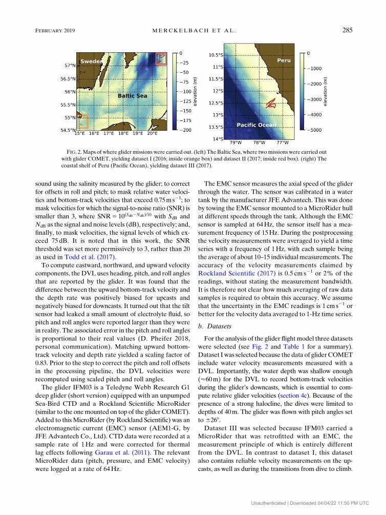
Dataset I was selected because the data of gliderCOMET

include water velocity measurements measured with a

DVL. Importantly, the water depth was shallow enough

(’60m) for the DVL to record bottom-track velocities

during the glider’s downcasts, which is essential to com-

pute relative glider velocities (section 4c). Because of the

presence of a strong halocline, the dives were limited to

depths of 40m. The glider was flown with pitch angles set

to 6268.Dataset III was selected because IFM03 carried a

MicroRider that was retrofitted with an EMC, the

measurement principle of which is entirely different

from the DVL. In contrast to dataset I, this dataset

also contains reliable velocity measurements on the up-

casts, as well as during the transitions from dive to climb.

FIG. 2.Maps of where glider missions were carried out. (left) The Baltic Sea, where twomissions were carried out

with glider COMET, yielding dataset I (2016; inside orange box) and dataset II (2017; inside red box). (right) The

coastal shelf of Peru (Pacific Ocean), yielding dataset III (2017).

FEBRUARY 2019 MERCKELBACH ET AL . 285

Unauthenticated | Downloaded 04/04/22 11:50 PM UTC

This glider was programmed to dive to 800m, or when

limited by topography to 15m above the seabed. From

this dataset we selected a sequence of profiles where the

glider dives to the full 800m. The glider was flown with

fixed battery positions, resulting in typical downcast and

upcast pitch angles of 328 and 288, respectively.Dataset II used the same glider setup as dataset I;

however, the glider was flown in water depths that were

too large to obtain bottom-track velocities for most of

the profiles. Hence, the DVL data from this dataset are

not used. This dataset is still of interest, because the day

prior to recovery was used to fly the glider for short

periods at two different pitch angles than the standard

268—namely, 6208 and 6308—in order to quantify the

effects of the induced drag.

c. Relative glider velocities from DVL measurements

The velocity profile data, configured to be outputted

by the DVL as eastward, northward, and upward ve-

locity components, represent the water velocity relative

to the glider. The first bin is found at 2.92m from the

transducer. However, the data from the first two bins

often show a signal that is distinctively different from the

other bins and therefore the first two bins are excluded

from the analysis to follow. The echoes from bins posi-

tioned farther away than about 15m were often weak,

not yielding a signal with a sufficiently high signal-to-

noise ratio. As a result, the typical range for which

meaningful data were obtained is some 7–15m away

from the glider. In the presence of significant vertical

shear, the relative velocity of the glider measured by the

DVL from a particular depth may not represent the

actual relative velocity at the depth of the glider. To

improve the estimates of the relative water velocity at

the glider’s position, we used the following approach.

Consider a glider collecting data using a downward-

looking DVL while diving (Fig. 3). When a profile en-

semble is collected, water velocities relative to the glider

are measured at a distance of about 10m below the

glider and turned into absolute water velocities by ac-

counting for the absolute glider velocity using the

bottom-track velocity. Some hundreds of seconds later,

assuming a nominal depth rate of 10 cm s21, the glider

reaches a depth at which it previously collected velocity

data. On the assumption that vertical changes in cur-

rents are much greater than horizontal changes, we

estimate the water velocity at the current glider’s depth

from previously collected profile ensembles and then

compute the relative glider velocity by subtracting the

glider absolute velocity (bottom-track velocity) at

this depth.

The drawback of this method is that in estimating the

water velocity components at the glider’s position, an

average is constructed from profile ensembles taken

100–200 s earlier. No tendencies, or ‘‘future’’ profile

ensemble data are taken into account. As an alternative,

we also implemented a simple Kalman filter. A Kalman

filter operates by propagating the mean and covariance

of a state using a dynamic model, in an optimal way,

given a time series of observations of the process (see,

e.g., Anderson and Moore 2005; Simon 2006). As for a

dynamicmodel we choose a simple one: the acceleration

of a current component (eastward, northward, or up-

ward) at a given depth is constant, with a model un-

certainty of s2 5 13 10216 m2 s24 to reflect the fact that

the model is only approximate in describing the real sys-

tem. The state vector consists of a velocity component at a

given depth and the corresponding acceleration. This filter

is run for each component and depth bin separately, using

measurements of the water velocity when they become

available. The variance of the measurement noise is esti-

mated at s2 5 0:0252 m2 s22; see also section 4a. The filter

is implemented as a forward–backward smoother, or a so-

called RTS filter after Rauch, Tung, and Striebel who

presented this filter in 1965; see Simon (2006). This filter is

first run forward and then backward in time, making

maximal use of available data.

In comparison with the Kalman filter, the averaging

method is much simpler to implement and is also compu-

tationally considerably more efficient. The Kalman filter

method, however, produces smoother, less noisy data and

has been used in the results reported in this work.

d. Incident water velocity from EMC measurements

The one-dimensional EMC sensor measures the ve-

locity component along the principal axis of the glider

(the j axis; see Fig. 1). Therefore, the incident water

velocity derived from this sensor UEMC relates to the

actual measured velocity UEMC, as

UEMC

5U

EMC

cos(a). (13)

TABLE 1. Dates and regions of the datasets used.

Dataset Glider Velocity sensor Region Start End

I COMET DVL Baltic Sea (southwest) 20 Jun 2016 26 Jun 2016

II COMET — Baltic Sea (central) 19 Oct 2017 28 Oct 2017

III IFM03 EMC Peru 29 Apr 2017 23 May 2017

286 JOURNAL OF ATMOSPHER IC AND OCEAN IC TECHNOLOGY VOLUME 36

Unauthenticated | Downloaded 04/04/22 11:50 PM UTC

Since a is not measured, values computed from the

steady-state model, for example, can be used instead.

These are generally small, so cos(a)5 11O (a2). How-

ever, it is noted that as a result of local shear, the angle of

attack may not always be small, leading to (13) being a

lower-bound estimate of the actual incident velocity.

During the processing of the EMC data, it was found that

the vertical water velocity computed from UEMC and the

glider’s pitch anglewas consistently larger inmagnitude than

the measured depth rate. In contrast to the glider COMET,

we have confidence in the pitch angles reported by glider

IFM03, as they were nearly identical to the pitch angles re-

ported by its MicroRider sensor. Therefore, we applied a

scaling factor to the velocities reported by the EMC so that

the difference between the vertical velocity component and

the depth rate vanishes. Using the angle of attack estimated

from the steady-state model (with lift angle and induced

drag settings found for glider COMET; see next section),

the factor was found to be equal to 0.93. A similar scaling

factor was found by the MircoRider’s manufacturer during

tests with a SeaExplorer glider with a built-in MicroRider

fitted with an EMC sensor, and an additionally mounted

ADCP (R. Lueck 2018, personal communication).

5. Glider flight model calibration and results

It is not possible to find optimal choices for both CD0

and a when using only the depth-rate measurement as

a model constraint; an additional velocity measurement

with a significant orthogonal (horizontal) component is re-

quired. In this section we use measurements of the incident

water velocity as an additionalmodel constraint to calibrate

for the lift angle coefficient. This is done first for the DVL

measurements and then for the EMC measurements.

Numerical values of drag and lift coefficients have a

meaning only, if referenced to a known surface area S

[see also (5) and (6)]. In this study we follow the con-

ventions used in aerodynamics and use the surface area

of the wings as reference area, giving S5 0:1 m2. An-

other choice for S could be the frontal area. To express

drag and lift coefficients, referenced to the frontal area,

the numerical values found in this study are to be mul-

tiplied by the ratio of wing area to frontal area.

In the subsections below, the value forCD1used by the

flight models is preset to 10.5 rad22, in anticipation of

the result presented at the end of this section, where we

also estimate the optimal value of CD1.

a. Lift angle coefficient

A simple approach is taken to estimate the optimal

value of a. To that end, an additional cost function R1 is

defined as

R15

1

N�N21

i50

(U[i]2UDVL

[i])2 , (14)

where UDVL[i] is the incident water velocity derived

from the DVL measurements with i. The cost function

FIG. 3. Construction of water current profiles, expressed in a geographic Cartesian reference frame, as measured

by a profiling glider. The dashed line represents the glider’s path. (left) Current profiles are measured during the

downcast only. (right) A zoomed-in view of the rectangle in the left panel. At t5 200 s, the glider (indicated by the

open circle) collects an absolute velocity profile, of which usable data are delineated by the dashed rectangle. Some

hundreds of seconds later, the absolute velocity at the depth of the glider (solid circle) can be estimated from

previousmeasurements (shaded rectangle). Subtracting the bottom-track velocity from the thus estimated absolute

velocity yields the relative velocity.

FEBRUARY 2019 MERCKELBACH ET AL . 287

Unauthenticated | Downloaded 04/04/22 11:50 PM UTC

R0 [(10)] is minimized for the parameter space

fCD0, mgg, for a range of preset values of a. Then, for

each triplet (CD0, mg, a), the cost functionR1 is evaluated.

Figure 4 summarizes the results of these successive

minimization steps, using the steady-state model (solid

lines) and the dynamic model (dashed lines) applied to

data from a subinterval of 4 h of data collected on

23 June 2017. The figure shows the optimal values for the

parasite drag coefficient and the mass (by minimizing

R0) for a range of preset values of a. It is seen that the

mass is independent of the value of the lift angle co-

efficient but that the drag coefficient is not. Moreover,

the steady-state model estimates lower values for CD0

than the dynamic model does, the explanation of

which is left for section 5c. The optimal value for a

(for which R1 is minimal) is found to be a’ 7:4 rad21,

for both models, where also the mean difference be-

tween the modeled and observed incident velocity is

approximately zero.

We can now repeat the procedure to determine the

glider flight model parameters CD0, mg, and a, but using

the EMC-derived incident velocity instead as the re-

quired nonvertical velocity component. The results are

shown in Fig. 5 and are found to be in line with the re-

sults obtained from the DVL data (cf. Fig. 4). The data

show a similar relationship between the optimized lift

and drag coefficients, and the mass appears to be in-

dependent of the lift angle coefficient. For this glider

(IFM03) an unbiased difference between measured and

modeled incident velocities is found for a5 7:5 rad21,

which is slightly higher than found for glider COMET.

In contrast to theDVL, the EMC provides continuous

velocity data on both the up- and downcasts, so that R0

can be modified to include a nonvertical velocity com-

ponent, yielding

R25

1

N�N21

i50

k

�U[i] sin(u[i]1a[i])1

dh

dt[i]

�2

1 (12 k)(U[i]2UEMC[i])2 , (15)

where k is a weighting coefficient, set to k5 1/2, giving

both velocity components equal importance assuming

that the accuracy of their measurements is similar. The

additional constraint allows for minimizing R2 for the

parameter tripletCD0,mg, and a simultaneously, yielding

CD05 0:136,mg 5 59:454 kg, and a5 7:7 rad21, indicated

by the cross symbols in Fig. 5.

The values for the lift angle coefficient, found for the

gliders COMET (DVL) and IFM03 (EMC), are only

slightly different. Figures 4 and 5 show, however, that

a variation in a of 1 rad21 would lead to a bias in the

incident velocity of approximately 6 and 3mms21 for

gliders COMET and IFM03, respectively. Given the

uncertainties in the velocity measurements, we consider

these findings to be consistent.

b. Induced drag coefficient

The induced drag coefficient CD1is another shape

parameter, the setting of which may influence the results

after calibrating themodel formg,CD0, and a. From (9) it

follows that the effect of the induced drag can be ab-

sorbed into the parasite drag coefficient if the glider is

flown with pitch angles that are similar in magnitude for

the up- and downcasts and (near) constant over time. In

most cases this is how gliders are operated, and this

second-order effect has little consequence on the model

FIG. 4. Dependency of mg and CD0on a (left ordinate axes), and corresponding mean and

standard deviations of the difference between the modeled and measured (DVL) incident

velocity as well asR1 (right ordinate axes). Results are shown for the steady-statemodel (solid

lines) and the dynamic model (dashed lines). The mean of the incident velocity difference is

denoted by mDU .

288 JOURNAL OF ATMOSPHER IC AND OCEAN IC TECHNOLOGY VOLUME 36

Unauthenticated | Downloaded 04/04/22 11:50 PM UTC

results. However, when operating gliders with micro-

structure sensors, the pitch battery position is usually

fixed to avoid vibrations that can interfere with shear

probe measurements during the moving of the pitch

battery. As a consequence, especially for deep glider

profiles, the pitch anglemay vary substantially as a result

of changes in the in situ water density and compression

of the hull, so changes in flight resulting from the in-

duced drag depend on the depth. The compressibility of

the hull also causes the flight to change with depth, and

hence it is difficult to distinguish between both effects.

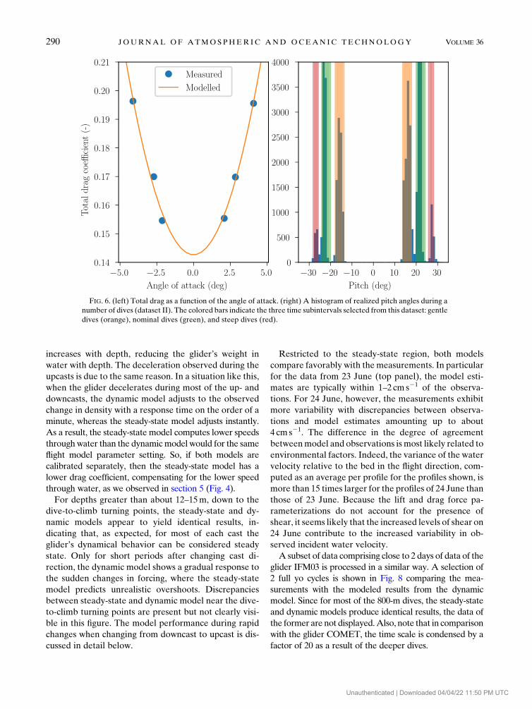
At the end of the glider experiment in dataset II, the

pitch settings of the glider COMET were varied. Over

the course of a day, the target pitch was changed to three

values—ut 5 168, 198, 278—where the absolute values of

the target pitch angles ut were the same for up- and

downcasts. Using a5 7:5 rad21 as found previously, the

glider flight model was calibrated for the mass and total

drag coefficient, CD 5CD01a2CD1

, for the three sub-

sets, each having a narrow range of pitch angles; see

Fig. 6, right panel. The optimization routine yields for

each pitch band a different value for CD. Since the angle

of attack can be assumed more or less constant within

each pitch band, CD can be plotted as a function of the

corresponding angle of attack; see the blue dots in Fig. 6,

left panel. As the induced drag effect is proportional to

the angle of attack squared, a parabola is fitted to the

data, yielding CD05 0:147 and CD1

5 10:5 rad22. The

value found for the induced drag coefficient is signifi-

cantly higher than the one estimated by Merckelbach

et al. (2010), who suggested a total value for the induced

drag of about 3 rad22. The discrepancy is most likely to

be due to the protruding features that the glider has,

such as the tail fin, the CTD, and, most importantly, the

Microrider package, which was not considered by

Merckelbach et al. (2010).

Like the parasite drag coefficient, the induced drag

coefficient is likely to change when the vehicle gets

biofouled. The value quoted here was determined for a

glider without noticeable biofouling. But, as argued

before, the effect caused by the induced drag is of

second-order importance, and some change in the in-

duced drag coefficient caused by biofouling is likely to

be insignificant.

c. Results

After calibrating the flight model for mass, parasite,

and induced drag coefficients, and lift angle coefficients

above, we use subsets of the data and solve both the

steady-state and dynamic model to yield time series of

incident water velocities. By comparing the time series

withmeasurements, we can assess themodel performance.

First, we compare the model results with measure-

ments obtained with the DVL for two subsets of about 4

and 9h of data, respectively. Measurements and model

results are shown in Fig. 7 for two intervals comprising

four full yos down to 40m of water depth spanning

about 30min on 23 June 2017 (top panels) and on

24 June 2017 (bottom panels), respectively. The incident

water velocity computed from the DVL measurements

is available only for water depths in excess of about 10m

and during downcasts. The DVL measurements (blue

curves, left panel) show that the glider quickly gains

speed when starting the downcast and then gradually

slows down as it gets deeper. This deceleration is also

reproduced in the incident water velocities computed by

the steady-state model (orange) and the dynamic model

(red). The reason for this is that the in situ density

FIG. 5. Dependency of mg and CD0on a (left ordinate axes), and corresponding mean and

standard deviations of the difference between the modeled and measured (EMC) incident

velocity as well as R1 (right ordinate axes). The cross symbols indicate the results of a

minimization of R2.

FEBRUARY 2019 MERCKELBACH ET AL . 289

Unauthenticated | Downloaded 04/04/22 11:50 PM UTC

increases with depth, reducing the glider’s weight in

water with depth. The deceleration observed during the

upcasts is due to the same reason. In a situation like this,

when the glider decelerates during most of the up- and

downcasts, the dynamic model adjusts to the observed

change in density with a response time on the order of a

minute, whereas the steady-state model adjusts instantly.

As a result, the steady-state model computes lower speeds

throughwater than the dynamicmodel would for the same

flight model parameter setting. So, if both models are

calibrated separately, then the steady-state model has a

lower drag coefficient, compensating for the lower speed

through water, as we observed in section 5 (Fig. 4).

For depths greater than about 12–15m, down to the

dive-to-climb turning points, the steady-state and dy-

namic models appear to yield identical results, in-

dicating that, as expected, for most of each cast the

glider’s dynamical behavior can be considered steady

state. Only for short periods after changing cast di-

rection, the dynamic model shows a gradual response to

the sudden changes in forcing, where the steady-state

model predicts unrealistic overshoots. Discrepancies

between steady-state and dynamic model near the dive-

to-climb turning points are present but not clearly visi-

ble in this figure. The model performance during rapid

changes when changing from downcast to upcast is dis-

cussed in detail below.

Restricted to the steady-state region, both models

compare favorably with themeasurements. In particular

for the data from 23 June (top panel), the model esti-

mates are typically within 1–2 cm s21 of the observa-

tions. For 24 June, however, the measurements exhibit

more variability with discrepancies between observa-

tions and model estimates amounting up to about

4 cm s21. The difference in the degree of agreement

betweenmodel and observations is most likely related to

environmental factors. Indeed, the variance of the water

velocity relative to the bed in the flight direction, com-

puted as an average per profile for the profiles shown, is

more than 15 times larger for the profiles of 24 June than

those of 23 June. Because the lift and drag force pa-

rameterizations do not account for the presence of

shear, it seems likely that the increased levels of shear on

24 June contribute to the increased variability in ob-

served incident water velocity.

A subset of data comprising close to 2 days of data of the

glider IFM03 is processed in a similar way. A selection of

2 full yo cycles is shown in Fig. 8 comparing the mea-

surements with the modeled results from the dynamic

model. Since for most of the 800-m dives, the steady-state

and dynamic models produce identical results, the data of

the former are not displayed.Also, note that in comparison

with the glider COMET, the time scale is condensed by a

factor of 20 as a result of the deeper dives.

FIG. 6. (left) Total drag as a function of the angle of attack. (right) A histogram of realized pitch angles during a

number of dives (dataset II). The colored bars indicate the three time subintervals selected from this dataset: gentle

dives (orange), nominal dives (green), and steep dives (red).

290 JOURNAL OF ATMOSPHER IC AND OCEAN IC TECHNOLOGY VOLUME 36

Unauthenticated | Downloaded 04/04/22 11:50 PM UTC

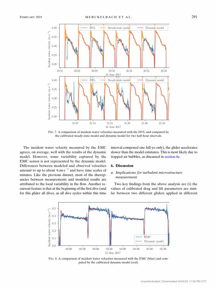
The incident water velocity measured by the EMC

agrees, on average, well with the results of the dynamic

model. However, some variability captured by the

EMC sensor is not represented by the dynamic model.

Differences between modeled and observed velocities

amount to up to about 4 cm s21 and have time scales of

minutes. Like the previous dataset, most of the discrep-

ancies between measurements and modeled results are

attributed to the local variability in the flow. Another re-

current feature is that at the beginning of the first dive (and

for this glider all dives, as all dive cycles within this time

interval composed one full yo only), the glider accelerates

slower than the model estimates. This is most likely due to

trapped air bubbles, as discussed in section 6c.

6. Discussion

a. Implications for turbulent microstructuremeasurement

Two key findings from the above analysis are (i) the

values of calibrated drag and lift parameters are simi-

lar between two different gliders applied in different

FIG. 7. A comparison of incident water velocities measured with the DVL and computed by

the calibrated steady-state model and dynamic model for two half-hour intervals.

FIG. 8. A comparison of incident water velocities measured with the EMC (blue) and com-

puted by the calibrated dynamic model (red).

FEBRUARY 2019 MERCKELBACH ET AL . 291

Unauthenticated | Downloaded 04/04/22 11:50 PM UTC

conditions, and (ii) the time series show good agree-

ment between the observed and modeled glider speed

through waterU. A question that naturally arises is what

errors a (calibrated) glider flight model then produces in

U, and what implications this has for estimates of the

dissipation rate from temperature and shear micro-

structure. These errors add to the uncertainty of the

dissipation rate measurements over that for standard

free-fall profilers, where the speed along the sensors is

estimated from the pressure rate of change. Although

not rigorously derived, the uncertainties of free-fall

profilers are generally estimated at a factor of approxi-

mately 2 (Dewey and Crawford 1988;Moum et al. 1995).

To estimate the errors produced from deviations in

the measured and modeled glider speeds, we first note

the scaling of the dissipation rate « with the flow speed

past the sensors, U. For « measured with airfoil shear

probes,

«515

2n

�›y

›x

�2

, (16)

where x represents the distance in the glider path di-

rection, y denotes across-path velocity fluctuations, n is

the kinematic viscosity, and the bar denotes a mean. The

probe returns a signal E(t) that is proportional to the lift

force on the probe (Uy), so we can express the across-

path velocities as y}E/U. Spatial gradients of y are then

found using Taylor’s frozen turbulence hypothesis,

whereby

›y

›x5

1

U

›y

›t}

1

U2

›E

›t. (17)

Therefore,

«}1

U4

�›E

›t

�2

, (18)

showing that « scales with the fourth power of the flow

speed past the sensors and that it will thus be sensitive to

errors in its estimation. Note that if « is measured by

using microstructure temperature sensors (Gregg 1999;

Ruddick et al. 2000), then «}U22 as a result of the lack

ofU dependence arising from the lift force in the case of

shear probes.

Errors in the estimation of « arising from deviations

between the glider flight model and the true speed

through water will therefore appear through the factor

(Umeas/Udyn)n, where n5 f2, 4g for measurements from

microstructure temperature sensors and shear probes,

respectively, and the U ratio corresponds to the mea-

sured speed to that obtained from the dynamic model.

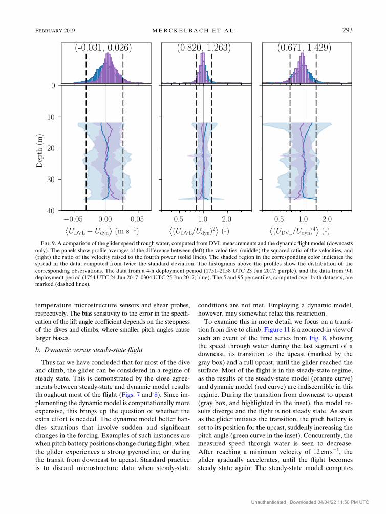
These factors are computed as profile averages (in-

dicated by angled braces) in Fig. 9 from the DVL da-

tasets. It shows averages as solid lines with the shaded

area indicating twice the standard deviation in the data

for both DVL datasets. Depths shallower than 12m are

not shown, since no reliable DVL data can be collected

(see also section 4c). Although some bias toward positive

or negative differences—amounting to close to 1cms21—

exists, the bias is not systematic, as it is different for two

consecutive deployments. When multiple deployments

are considered, there is negligible bias in the difference

between mean measured and modeled speeds.

The histograms in Fig. 9 show that 90% of the errors

expected in dissipation rate estimates as a result of

modeled glider speeds are within a factor of 0.67–1.43

for shear probe measurements (n5 4) and within 0.82–

1.26 for temperature microstructure (n5 2). These er-

rors should be compared to the factor-of-2 uncertainty

normally associated with dissipation rate measurements

from vertical profilers (Dewey and Crawford 1988;

Moum et al. 1995). In addition, it is not clear how much

of this difference between modeled and measured

speeds can be attributed to the need to use DVL mea-

surements that are not coincident in time and space with

the glider position, and require averaging to reduce

measurement noise.

An advantage the EMC sensor has over the DVL is

that it measures velocities collocated in time and space

with the glider flight model. As long as the instanta-

neous angle of attack remains small, themeasured quantity

represents the glider speed through water, an assumption

we havemade in the analysis. The same profile averaged

quantities as in Fig. 9, but now for the EMC sensor, are

shown in Fig. 10. For depths deeper than 150m, we also

find unbiased results, with error ratios that have a

smaller spread than for the DVL [i.e., 90% of the data

lie in the ranges of 0:83, h(UEMC/Udyn)4 , 1:20 and

0:91, h(UEMC/Udyn)2 , 1:09]. The velocity measure-

ments made by the EMC sensor have a standard de-

viation that is about an order of magnitude smaller than

the readings from the DVL (section 4a), so this suggests

that a fraction of the spread of the data observed for the

DVL (and possibly also for the EMC) could be due to

uncertainty in the measurements.

If the steady-state model were applied to the pres-

ent data but using a lift angle coefficient of 6.1 rad21

(Merckelbach et al. 2010), then the bias in the differ-

ence between measured and modeled incident veloci-

ties would be 1.3 and 0.5 cm s21 for datasets I (Fig. 4)

and III (Fig. 5), respectively. The associated biases

in the estimates for the dissipation rate applied to

dataset I (dataset III) would an underestimation of a

factor of 1.10 (1.05) and 1.20 (1.07) for estimates from

292 JOURNAL OF ATMOSPHER IC AND OCEAN IC TECHNOLOGY VOLUME 36

Unauthenticated | Downloaded 04/04/22 11:50 PM UTC

temperature microstructure sensors and shear probes,

respectively. The bias sensitivity to the error in the specifi-

cation of the lift angle coefficient depends on the steepness

of the dives and climbs, where smaller pitch angles cause

larger biases.

b. Dynamic versus steady-state flight

Thus far we have concluded that for most of the dive

and climb, the glider can be considered in a regime of

steady state. This is demonstrated by the close agree-

ments between steady-state and dynamic model results

throughout most of the flight (Figs. 7 and 8). Since im-

plementing the dynamic model is computationally more

expensive, this brings up the question of whether the

extra effort is needed. The dynamic model better han-

dles situations that involve sudden and significant

changes in the forcing. Examples of such instances are

when pitch battery positions change during flight, when

the glider experiences a strong pycnocline, or during

the transit from downcast to upcast. Standard practice

is to discard microstructure data when steady-state

conditions are not met. Employing a dynamic model,

however, may somewhat relax this restriction.

To examine this in more detail, we focus on a transi-

tion from dive to climb. Figure 11 is a zoomed-in view of

such an event of the time series from Fig. 8, showing

the speed through water during the last segment of a

downcast, its transition to the upcast (marked by the

gray box) and a full upcast, until the glider reached the

surface. Most of the flight is in the steady-state regime,

as the results of the steady-state model (orange curve)

and dynamic model (red curve) are indiscernible in this

regime. During the transition from downcast to upcast

(gray box, and highlighted in the inset), the model re-

sults diverge and the flight is not steady state. As soon

as the glider initiates the transition, the pitch battery is

set to its position for the upcast, suddenly increasing the

pitch angle (green curve in the inset). Concurrently, the

measured speed through water is seen to decrease.

After reaching a minimum velocity of 12 cm s21, the

glider gradually accelerates, until the flight becomes

steady state again. The steady-state model computes

FIG. 9. A comparison of the glider speed through water, computed from DVLmeasurements and the dynamic flight model (downcasts

only). The panels show profile averages of the difference between (left) the velocities, (middle) the squared ratio of the velocities, and

(right) the ratio of the velocity raised to the fourth power (solid lines). The shaded region in the corresponding color indicates the

spread in the data, computed from twice the standard deviation. The histograms above the profiles show the distribution of the

corresponding observations. The data from a 4-h deployment period (1751–2158 UTC 23 Jun 2017; purple), and the data from 9-h

deployment period (1754 UTC 24 Jun 2017–0304 UTC 25 Jun 2017; blue). The 5 and 95 percentiles, computed over both datasets, are

marked (dashed lines).

FEBRUARY 2019 MERCKELBACH ET AL . 293

Unauthenticated | Downloaded 04/04/22 11:50 PM UTC

false behavior during the transition. The dynamic model,

however, does reproduce the dip in speed.

c. Flight model error sources

Although errors in the velocity measurements lead to

discrepancies between measured and modeled incident

velocities, some of these discrepancies can be related to

the model failing to capture all aspects of the glider

flight. For water depths less than 150m, discrepancies

between observed and modeled velocities are very

clearly present in the dataset of glider IFM03 (Fig. 10). It

is unlikely that these discrepancies can be related to

inaccurate velocity measurements. It is, however, a

known issue for Slocum gliders with an oil-based dis-

placement pump, such as the glider IFM03, that air can

diffuse into the oil system. Air bubbles in the oil system

will lead to inaccurate reporting of the actual glider

volume change, causing the flight model to compute

erroneous buoyancy forces and as a result erroneous

flight velocities. Because there is currently no way to

measure how much air is present, and where it resides,

this aspect is not included in the flight model. The effect

of air bubbles can be identified by comparing the com-

puted vertical glider velocities with the observed depth

rate; if calibrated for deep dives, the presence of air

bubbles manifests itself as a bias in the vertical velocity

difference during the shallower part of the dives.

A further assumption underlying both the steady-

state and dynamic flight models is that the ocean cur-

rents are steady and free of shear. The consequence is

that in the presence of, for example, vertical shear and

internal waves with short periods, the inertia of the

glider can cause the instantaneous incident velocity to

be significantly different from the modeled incident

velocity, introducing errors in the drag and lift forces

computed by the model. Unfortunately, this issue is not

remedied by the dynamic model developed herein, de-

spite having the inertial terms included. This is because

the model cannot discern between the glider velocity in

an inertial frame, the time derivative of which equals the

acceleration, and the incident water velocity (relative to

the glider), which is used in the parameterizations of the

lift and drag forces. The results shown in Figs. 7 and 8

indicate that the discrepancies observed between the

FIG. 10. A comparison of the glider speed throughwater, computed fromEMCmeasurements and the dynamic flightmodel. The panels

show profile averages of the difference between (left) the velocities, (middle) the squared ratio of the velocities, and (right) the ratio of the

velocity raised to the fourth power (solid lines). The shaded region in the corresponding color indicates the spread in the data, computed

from twice the standard deviation. The downcasts (blue) and upcasts (red) are indicated. The histograms above the profiles show the

distribution of the corresponding observations. The 5 and 95 percentiles, computed over both the down- and upcasts combined, are

marked (dashed lines). The data encompass a 45-h period (0020 UTC 12 May–2113 UTC 13 May 2017).

294 JOURNAL OF ATMOSPHER IC AND OCEAN IC TECHNOLOGY VOLUME 36

Unauthenticated | Downloaded 04/04/22 11:50 PM UTC

measured incident velocities and the dynamic model

results occur on time scales on the order of 1–10min,

and are likely caused by the model failing to capture

the effects caused by an unsteady ocean.

The present measurements suggest that the steady

ocean assumption introduces errors in the estimates of

the dissipation rate that are within acceptable levels

given the current uncertainties in microstructure esti-

mates. This may not be true anymore for more dynamic

environments than those encountered in this study, so in

those conditions measuring the dissipation rate with an

acceptable accuracy may still require direct measure-

ments of the glider flight.

7. Conclusions

This study is the first to use measurements of in situ

glider flight to test, calibrate, and extend a glider flight

model. Our principal motivation is to quantify and

reduce uncertainties in the use of flight models for tur-

bulent microstructure studies. Calibration of the steady-

state model of Merckelbach et al. (2010) resulted in

changes in the lift angle coefficient to a5 7:5 rad21 as

well as the induced drag coefficient CD15 10:5 rad21.

This change in the value of the lift angle coefficient from

that reported in Merckelbach et al. (2010) results in a

reduction of the difference between measured and

modeled incident water velocities of about 0.5–1.3 cms21.

Measurements of in situ glider flight allow us to quantify

errors in dissipation rate calculations associatedwith errors

in the incident water velocity predicted by the flightmodel.

Using velocities from theEMCas a baseline, we found that

90% of the estimates of the dissipation rate based on the

calibrated flight model are within a factor of 1.1 and 1.2 for

measurements derived from microstructure temperature

sensors and shear probes, respectively. The uncalibrated

model would produce a bias of factors of 1.05–1.10 and

1.07–1.20 for temperature and shear microstructure, re-

spectively. The uncertainty in dissipation rate estimates

can be attributed to the local variability in the flow, which

is not accounted for in the flight model, as well as possible

noise from the velocity measurement itself. When using

water velocities measured with the DVL, for which the

estimates are more prone to instrument noise, the factors

are slightly larger, namely, 1.2 and 1.4, respectively.

To better represent the hydrodynamics, we have ex-

tended the steady-state glider flight model ofMerckelbach

et al. (2010) to a dynamic model by including the inertial

and added mass terms. A comparison of the two models

found that the flight is largely well described by the

steady-state model and that only when conditions change

rapidly, such as during dive–climb transitions, does the

steady-state model fail, whereas the dynamic model pre-

dicts the incident water velocity reasonably well.

Acknowledgments. We are grateful to Rolf Lueck

(Rockland Scientific) for the useful discussion on the

interpretation of the velocities measured with the elec-

tromagnetic currentmeter.We also thankDavid Pheifer

(True North Technologies) for sharing his expertise on

how to correct the attitude data of glider COMET. The

bathymetry data used in this work were provided by

GEBCO (www.gebco.net). This paper is a contribution

to the projects M6 and T2 of the Collaborative Research

FIG. 11. A section of a time series showing the speed through water as measured by the

EMC (blue curve), the steady-state model (orange), and a dynamic glider flight model (red).

The inset is a zoomed-in view of a deep transition from dive to climb.

FEBRUARY 2019 MERCKELBACH ET AL . 295

Unauthenticated | Downloaded 04/04/22 11:50 PM UTC

Centre TRR 181, ‘‘Energy Transfer in Atmosphere and

Ocean’’; and the projectB6of theCollaborativeResearch

Centre SFB 754, ‘‘Climate–Biogeochemistry Interactions

in the Tropical Ocean’’—all funded by the German Re-

search Foundation (Deutsche Forschungsgemeinschaft).

Part of the measurements (dataset I) took place during

the Expedition Clockwork Ocean, which was partially

supported by the Helmholtz-Zentrum Geesthacht as

part of its PACES II program.We thank the captain and

crew of the R/V Elisabeth Mann Borgese for the excel-

lent technical support, and express our appreciation for

the constructive comments and suggestions by two anon-

ymous reviewers. The data used in this manuscript are

available online (https://doi.org/10.5281/zenodo.2270123).

REFERENCES

Anderson, B. D. O., and J. B. Moore, 2005:Optimal Filtering.Dover

Books on Electrical Engineering, Dover Publications, 368 pp.

Dewey, R., and W. Crawford, 1988: Bottom stress estimates from

vertical dissipation rate profiles on the continental shelf.

J. Phys. Oceanogr., 18, 1167–1177, https://doi.org/10.1175/

1520-0485(1988)018,1167:BSEFVD.2.0.CO;2.

Fer, I., A. K. Peterson, and J. E. Ullgren, 2014: Microstructure

measurements from and underwater glider in the turbulent

FaroeBankChannel overflow. J. Atmos. Oceanic Technol., 31,

1128–1150, https://doi.org/10.1175/JTECH-D-13-00221.1.

Garau, B., S. Ruiz,W. G. Zhang, A. Pascual, E. Heslop, J. Kerfoot,

and J. Tintoré, 2011: Thermal lag correction on Slocum CTD

glider data. J. Atmos. Oceanic Technol., 28, 1065–1071, https://

doi.org/10.1175/JTECH-D-10-05030.1.

Gregg, M., 1999: Uncertainties and limitations in measuring « and

xT . J. Atmos. Oceanic Technol., 16, 1483–1490, https://doi.org/10.1175/1520-0426(1999)016,1483:UALIMA.2.0.CO;2.

Griffiths, G., Ed., 2002:Technology andApplications of Autonomous

Underwater Vehicles. Ocean Science and Technology Series,

CRC Press, 368 pp., https://doi.org/10.1201/9780203522301.

Imlay, F. H., 1961: The complete expressions for ‘‘addedmass’’ of a

rigid body moving in an ideal fluid. David Taylor Model Basin

Research and Development Rep. 1528, 31 pp.

Merckelbach,L., 2018a:Aglider flightmodel for Slocumoceangliders.

GitHub, https://github.com/smerckel/gliderflight/tree/1.0.1.

——, 2018b: Initial release of glider flight model. Version 1.0.1,

Zenodo, https://doi.org/10.5281/zenodo.2222694.

——, D. Smeed, and G. Griffiths, 2010: Vertical velocities from

underwater gliders. J. Oceanic Atmos. Technol., 27, 547–563,

https://doi.org/10.1175/2009JTECHO710.1.

Moum, J., M. Gregg, R. Lien, and M. Carr, 1995: Comparison of

turbulence kinetic energy dissipation rate estimates from two

ocean microstructure profilers. J. Atmos. Oceanic Technol.,

12, 346–366, https://doi.org/10.1175/1520-0426(1995)012,0346:

COTKED.2.0.CO;2.

Newman, J. N., 1977: Marine Hydrodynamics. MIT Press, 402 pp.,

https://doi.org/10.7551/mitpress/4443.001.0001.

Palmer,M., G. Stephenson,M. Inall, C. Balfour, A. Düsterhus, andJ.Green, 2015: Turbulence andmixing by internal waves in the

Celtic Sea determined from ocean glider microstructure

measurements. J. Mar. Syst., 144, 57–69, https://doi.org/10.1016/

j.jmarsys.2014.11.005.

Peterson, A. K., and I. Fer, 2014: Dissipation measurements using

temperature microstructure from an underwater glider.Methods

Oceanogr., 10, 44–69, https://doi.org/10.1016/j.mio.2014.05.002.

Rockland Scientific, 2017: MicroPod-EM: Electromagnetic flow

sensor. Rockland Scientific Rep., 2 pp., https://rocklandscientific.

com/wp-content/uploads/2017/05/RSI-Data-Sheet-MicroPodEM-

A4-1_00-web.pdf.

Ruddick, B., A. Anis, and K. Thompson, 2000: Maximum likeli-

hood spectral fitting: The Batchelor spectrum. J. Atmos.

Oceanic Technol., 17, 1541–1555, https://doi.org/10.1175/1520-

0426(2000)017,1541:MLSFTB.2.0.CO;2.

Rudnick, D., 2016: Ocean research enabled by underwater gliders.

Annu. Rev. Mar. Sci., 8, 519–541, https://doi.org/10.1146/

annurev-marine-122414-033913.

Scheifele, B., S. Waterman, L. Merckelbach, and J. Carpenter,

2018: Measuring the dissipation rate of turbulent kinetic en-

ergy in strongly stratified, low-energy environments: A case

study from the Arctic Ocean. J. Geophys. Res. Oceans, 123,

5459–5480. https://doi.org/10.1029/2017JC013731.

Schultze, L. K. P., L. M. Merckelbach, and J. R. Carpenter, 2017:

Turbulence and mixing in a shallow stratified shelf sea from

underwater gliders. J. Geophys. Res. Oceans, 122, 9092–9109,

https://doi.org/10.1002/2017JC012872.

Simon, D., 2006: Optimal State Estimation: Kalman, H‘, and

Nonlinear Approaches. Wiley and Sons, 526 pp.

St. Laurent, L., and S. Merrifield, 2017: Measurements of near-surface

turbulence and mixing from autonomous ocean gliders. Ocean-

ography, 30 (2), 116–125, https://doi.org/10.5670/oceanog.2017.231.Teledyne RD Instruments, 2017: Explorer Doppler velocity log

(DVL): Navigation performance in a compact package. Teledyne

RD Instruments Rep., 2 pp., http://www.teledynemarine.com/

Lists/Downloads/explorer_datasheet_hr.pdf.

Todd, R., D. Rudnick, J. Sherman, W. Owens, and L. George,

2017: Absolute velocity estimates from autonomous under-

water gliders equipped with Doppler current profilers.

J. Atmos. Oceanic Technol., 34, 309–330, https://doi.org/10.1175/

JTECH-D-16-0156.1.

Wolk, F., R. Lueck, and L. St. Laurent, 2009: Turbulence mea-

surements from a glider. Proc. 13th Workshop on Physical

Processes in Natural Waters, Palermo, Italy, University of

Palermo, https://rocklandscientific.com/wp-content/uploads/

2015/01/Wolk_Lueck_StLaurent_final_PPNW.pdf.

296 JOURNAL OF ATMOSPHER IC AND OCEAN IC TECHNOLOGY VOLUME 36

Unauthenticated | Downloaded 04/04/22 11:50 PM UTC