Uludag University Journal of The Faculty of Engineering, Vol. 22, No.1, 2017 RESEARCH DOI: 10.17482/uumfd.308630

103

A COMPARISON OF ATMOSPHERIC CORRECTION METHODS

ON HYPERION IMAGERY IN FOREST AREAS

Mufit CETIN *

Nebiye MUSAOGLU **

Osman Hilmi KOCAL*

Received: 26.02.2016; revised: 05.12.2016; accepted: 28.02.2017

Abstract: The reflectance values recorded by Earth observing satellite sensors can be different from the

surface reflectance values measured on the ground due to interference of gases and water vapor in the

atmosphere. Therefore, atmospheric correction is a significant procedure to derive the true surface

reflectance value during the processing of remotely sensed imagery especially with hyperspectral data. In

this context, this study attempts to analyze the quality of the surface reflectance derived from EO-1

Hyperion hyperspectral imagery using the atmospheric radiative transfer (RT) models (FLAASH and

ATCOR) and empirical line (EL) method. In the study, ground-based reflectance measurements derived

from ASD FieldSpec spectroradiometer are used as reference to evaluate the quality of the retrieved

surface reflectance. The results showed that EL and ATCOR methods achieved the best results for

reducing some of the atmospheric effects, but FLAASH method resulted in strong anomalies in the

corrected reflectance.

Keywords: Satellite Image, Hyperspectral, Hyperion, Atmospheric Correction.

HYPERION Görüntüsü ile Atmosferik Düzeltme Yöntemlerinin Karşılaştırılması:Orman Alanı

Örneği

Öz: Uzaktan algılama amaçlı algılayıcılar tarafından elde edilen yansıma değerleri atmosferik etkilerden

dolayı hatalar içermektedir. Dolayısıyla, özellikle hiperspektral uydu görüntülerinin işlenmesinde ve

analizinde doğru sonuçlar elde edilmesi için atmosferik düzeltme önemli bir işlemdir. Bu kapsamda, EO-

1 Hyperion hiperspektral uydu görüntüsü kullanılarak atmosferik ışınımsal transfer modelleri (FLAASH,

ATCOR) ve Doğrusal Ampirik (EL) yöntemi kullanılarak performans sonuçları sunulmuştur. Elde edilen

düzeltilmiş verilerin kalite analizi ASD spektroradyometre aleti ile yapılan yer ölçmeleri kullanılarak

gerçekleştirilmiştir. Çalışmada elde edilen sonuçlara göre EL ve ATCOR yöntemlerinin atmosferik

etkinin giderilmesinde en iyi sonuçları verdiği, FLAASH yönteminin ise düzeltilmiş reflektans eğrilerinde

güçlü sapmalara neden olduğu görülmüştür.

Anahtar Kelimeler: Uydu görüntüsü, Hiperspektral, Hyperion, Atmosferik düzeltme.

1. INTRODUCTION

Spaceborne remote sensing is an efficient and relatively inexpensive way as compared to

the conventional ground-based methods for the mapping of land covers, especially at regional

and national levels. Hyperspectral imaging, which is one of the technological developments in

remote sensing, opens new possibilities to detect particular types of earth surface materials. The

hyperspectral systems generate hundreds of discrete, contiguous spectral narrow bands than the

* Yalova University, Department of Computer Engineering, Tigem Campus Yalova, 77200, TURKEY ** Istanbul Technical University, Department of Geomatic Engineering, Maslak/Istanbul, 34469, TURKEY

Correspondence Author: Mufit Cetin (mufit.cetin@yalova.edu.tr)

Cetin M.,Musaoglu N.,Koçal O:H.: A Comp.of Atmospheric Corr. Meth. on Hyp. Imagery in Forest Areas

104

multispectral sensors which are most commonly used in remote sensing applications. For that

reason, hyperspectral remote sensing has wide range of scientific and technical applications in

forestry, agriculture, geology and environmental management such as mineral exploration,

predictions of crop yield, detection of vegetation stress and soil mapping (Hardin and Hardin,

2013; Shang and Chisholm, 2014; Lee and others, 2014; Schmid and others, 2016).

Using of raw hyperspectral satellite images directly is not very convenient to retrieve

reflectance values of the ground materials in the specific applications of remote sensing due to

atmospheric effects and sensor sensitivity. Therefore, radiometric calibration and atmospheric

correction are significant procedures to create a consistent surface reflectance from the

hyperspectral data (Guanter and others, 2007a). A number of atmospheric correction methods

have been developed based on radiative transfer codes (i.e. LOWTRAN and MODTRAN) in

literature such as ATREM (Gao and others,1993), FLAASH (Matthew and others, 2000),

ACORN (Miller, 2002), HATCH (Qu and others, 2003) and ATCOR (Richter, 1996). Various

studies are conducted to evaluate the performance of atmospheric correction methods for

different remotely sensed images such as Landsat TM (Lu and others, 2002; Norjamäki and

Tokola, 2007), AVIRIS (Airborne Visible/Infrared Imaging Spectrometer) (Farrand and others,

1994; Veraguth and others, 1995), IKONOS (Karpouzli and Malthus, 2003; Xu and Huang,

2008) and others (Dwyer and others, 1995; Perry and others, 2000).

In this study, both qualitative and quantitative spectral analysis on Hyperion imagery are

implemented to compare three common methods including Empirical Line (EL), Atmospheric

correction (ATCOR) and Fast Line-of-sight Atmospheric Analysis of Spectral Hypercubes

(FLAASH). The field reflectance measurements are obtained from known locations

simultaneously with an Analytical Spectral Devices (ASD) Fieldspec Pro spectroradiometer in

order to perform the spectral quality analysis of the methods. The results showed that EL and

ATCOR methods achieved the best results for reducing some of the atmospheric effects, but

FLAASH method is caused to strong anomalies in the corrected reflectance.

2. DATA

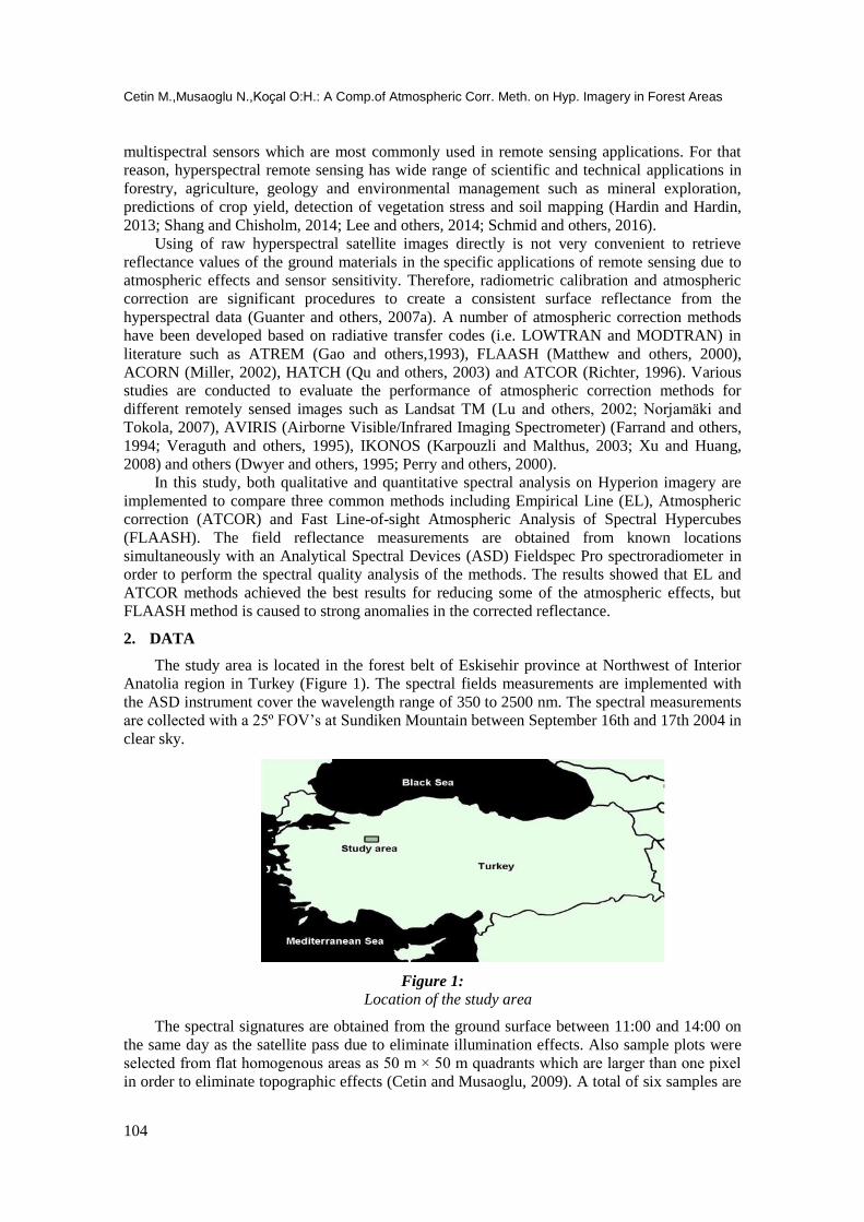
The study area is located in the forest belt of Eskisehir province at Northwest of Interior

Anatolia region in Turkey (Figure 1). The spectral fields measurements are implemented with

the ASD instrument cover the wavelength range of 350 to 2500 nm. The spectral measurements

are collected with a 25º FOV’s at Sundiken Mountain between September 16th and 17th 2004 in

clear sky.

Figure 1:

Location of the study area

The spectral signatures are obtained from the ground surface between 11:00 and 14:00 on

the same day as the satellite pass due to eliminate illumination effects. Also sample plots were

selected from flat homogenous areas as 50 m × 50 m quadrants which are larger than one pixel

in order to eliminate topographic effects (Cetin and Musaoglu, 2009). A total of six samples are

Uludag University Journal of The Faculty of Engineering, Vol. 22, No.1,2017

105

used in the study, including water, stubble field, pasture, one deciduous (oak) and two

coniferous species (Pinus sylvestris and Pinus nigra).

The hyperspectral data were acquired by EO-1 Hyperion sensor on September 17, 2004,

around 10:30 a.m. local time. EO-1 spacecraft has two types of optic sensors that include the

Advanced Land Imager (ALI) and Hyperion. EO-1 satellite can collect both high-resolution

panchromatic (PAN) and low-resolution multispectral (MS) images simultaneously by using

ALI sensor and hyperspectral image gathered using Hyperion sensor. Hyperion scenes cover

just about 7.7 km in the across-track direction, and 42 km in the along-track direction on the

ground. The Hyperion image contains 242 channels ranging from 356 to 2577 nm in 10 nm

spectral and 30 m spatial resolutions (Cetin and Musaoglu, 2009; Pearlman et al., 2003).

3. METHODOLOGY

The methodology for retrieving reflectance spectra from Hyperion imagery consists of the

following three main steps including radiometric, geometric and atmospheric corrections. The

radiometric errors such as destriping and smile effects generally occur in the Hyperion dataset

due to the internal effects of the sensor such as miscalibration of the detector and noise of the

system. All the methodological steps are illustrated in Figure 2.

Figure 2:

The flow diagram for retrieval of surface reflectance values.

3.1. Radiometric Correction

3.1.1. Exclusion of Bad Bands

EO-1 Hyperion Level 1 Radiometric product contains only 198 calibrated bands include 8-

57 for the VNIR and 77-224 for the SWIR due to the detectors' low responsivity. Band 56

Cetin M.,Musaoglu N.,Koçal O:H.: A Comp.of Atmospheric Corr. Meth. on Hyp. Imagery in Forest Areas

106

(915.23 nm) and band 57 (925.41 nm) in VNIR with band 77 (912.45 nm) and band 78 (922.54

nm) in SWIR are overlapped. Only 196 unique channels remained when un-calibrated bands

with band 77 and 78 are removed. Water absorption bands in 1340-1450 nm and 1750-1970 nm

are eliminated. In this study, the EO-1 Hyperion image is visually inspected band by band to

eliminate spectral channels whose signals were significantly affected by atmospheric absorption

windows and low signal to noise ratio (Christian and Krishnayya, 2007).The defective bands are

excluded 1-7, 58-78, 119 – 130, 164 – 186, and 217 – 224, namely and 153 healthy bands are

remained for analysis (Table 1). EO-1 Hyperion Level 1R product include some sensor related

artifacts such as vertical striping and smile effects are corrected before image fusion

(Goodenough and others, 2003).

Table 1. The spectral bands used in the Hyperion data sets

Detectors Bands Wavelength (nm) Number of bands

VNIR 8–57 426 – 926 50

SWIR

79 – 118 933 – 1326 40

131 – 163 1457 – 1780 33

187 – 216 2022 – 2315 30

Total used bands 153

3.1.2. Destriping

Vertical-striping is usually occurs in the image acquired using pushbroom sensors such as

Airborne Visible/Infrared Imaging Spectrometer and Hyperion due to various effects such as

detector nonlinearities, movement of the slit with respect to the focal plane and temperature

effects (Kruse and others, 2003). First, vertical stripes should be removed before the analysis of

the Hyperion image and eliminated to provide accurate radiometric calibration (Goetz and

others, 2003). Therefore, the mean of each column per image was calculated and the quality

control is performed by inspecting visually.

3.1.3. Smile Correction

The spectral shift errors caused by the large spectral artifacts in the atmospheric absorption

regions. A spectral shift in the size of 0.1 nm for the band center with Full Width at Half

Maximum (FWHM) of 10 nm can be caused to 5% difference in the reflectance values (Goetz

and others, 2003; Guanter and others, 2007b). Moreover, some studies showed that the spectral

shift errors can reach up to 20% in the NIR region and 50% in the atmospheric absorption bands

close to 1400 and 1900 nm due to strong water vapor absorption (Cocks and others, 1998;

Guanter and others, 2006). Prior to atmospheric correction, this spectral shift effect has to be

corrected to retrieve the proper surface reflectance values. Therefore, a weighted linear

interpolation method is performed on each column of the hyperspectral data using the auxiliary

spectral calibration table (smile table), extracted from the header file of Level 1R product.

The "weighted linear interpolation" can be thought as "moving linear interpolation" in

spectral direction, which is performed with the following formula:

(1)

where d is the real DN at the nominal band centre wavelength w, which is in header file;

d(i) is the DN at wavelength w(i), which is in smile table;

d(i+1) is the DN at wavelength w(i+1), which is in smile table. w is usually between w(i)

and w(i+1).

Uludag University Journal of The Faculty of Engineering, Vol. 22, No.1,2017

107

Figure 3:

MNF band 1 of VNIR and SWIR bands, corrected spectral curvature effects (smile)

Figure 3 shows minimum noise fraction (MNF) transform of VNIR bands. First MNF band

represents brightness gradients due to smile effect for Hyperion images. On the other hand, this

brightness gradient is not observed in the SWIR region. Hyperion data, applied for the weighted

linear interpolation to reduce the smile effects, is examined in MNF space to evaluate the smile

correction results. But the results show that improved imagery still contains cross-track

brightness gradients.

3.2. Geometric Correction

Firstly, Hyperion imagery is orthorectified by using digital elevation model (DEM) created

from 1:25 000 scaled topographic maps, with 19 Ground Control Points (GCPs) and 7

Independent Check Points (ICPs). The Root Mean Square (RMS) residuals of the GCPs are 0.39

pixels in X, 0.40 pixels in Y directions and 0.55 pixels in total, respectively. The RMS errors of

the ICPs are 0.37 pixels, 0.58 pixels and 0.69 pixels in X, Y directions and in total, respectively.

The nearest neighbor resampling method is used to preserve the original values in the image

rectification (Cetin and Musaoglu, 2009).

3.3. Atmospheric Correction

The main objective of atmospheric correction methods is to reduce atmospheric effects in

order to retrieve more accurate surface reflectance values from the satellite images. Methods can

be divided into two broad categories including relative and absolute techniques. Also, the

relative atmospheric correction method consists of three sub-groups include flat field method,

internal average relative reflectance model and empirical line method. Relative atmospheric

correction methods utilize some statistical information extracted from images and priori

a. VNIR b. SWIR

Cetin M.,Musaoglu N.,Koçal O:H.: A Comp.of Atmospheric Corr. Meth. on Hyp. Imagery in Forest Areas

108

knowledge of the ground surfaces obtained from field measurements. On the other hand, the

absolute atmospheric correction methods needs some inputs such as solar geometry (azimuth,

elevation), sensor geometry (zenith, azimuth), scene centrel location, aerosol model (rural,

urban, etc), atmospheric condition and time of image acquisition. Therefore, each of the

atmospheric correction methods has their own benefits and challenges according to the aim and

opportunities of the research (Gao and others, 1993; Guanter and others, 2007a; Mahiny and

Turner, 2007; Cetin and Musaoglu, 2008; San and Suzen, 2010).

3.3.1.1. Empirical Line Method

This method suggest that there is linear relationship between the spectral radiance values

observed by the sensor and the spectral reflectance values obtained from the ground field

spectrometer for each of the calibration objects within each band of the remotely sensed image.

Atmospherically corrected images can be produced applying this extracted linear relationship to

remotely sensed data (Smith and Milton, 1999). The EL method is based on the the linear

regression model as fllows:

(2)

where is the spectral radiance for a given pixel in spectral band i, is the reflectance

value of the sample, and coefficients are slope and intercept derived from band i by the

linear regression model, respectively.

The coefficients can be determined by using the Eq.(2). Field measurements of calibration

objects are the most important stage to obtain the valid and accurate results in EL method. The

field measurements of the calibration objects have to be done at the same time with satellite

overpass. This method assumes that all study area has the same atmospheric conditions and no

topographic effect. Besides, selected sample areas should be flat, homogeneous and a few pixels

in size. Various studies are conducted to calibrate remotely sensed data using empirical line

method especially for broad band images (Farrand and others, 1994; Karpouzli and Malthus,

2003; Xu and Huang, 2008). As in many atmospheric calibration studies in the literature, the

water and stubble sample areas as the dark and light calibration targets for spectral calibration

depending on the number of selected samples. Thus, the linear equation is used to predict the

reflectance of other targets on the image. Moreover, additional field spectral measurements are

carried out to evaluate the performance of the atmospheric correction methods.

3.3.1.2. Radiative Transfer Models

It can be modeled using the radiative transfer codes to reduce the scattering, water vapor

absorptions and transmission properties of the atmosphere without field measurements or priori

knowledge. In literature, radiative transfer models are more commonly used than the relative

correction techniques (especially flat field and internal average relative reflectance) since they

provide more accurate results (Goetz and others, 2002). Radiative transfer models are based on

the following simple expression:

(3)

where the radiance value is acquired by a sensor, is the atmospheric path radiance

computed by radiative transfer model and is corrected radiance value for a given pixel in

the satellite image.

In this study, ATCOR and FLAASH atmospheric models, based on MODTRAN-4

radiative transfer code, are used to evaluate the results of the corrected images using the field

spectral measurements and to compare with relative atmospheric methods. For accomplising

this, we have inserted some parameters to the model that include sensor altitude, wavelength

date, Full Width Half Maximum (FWHM), time, season, latitude/longitude of study area,

Uludag University Journal of The Faculty of Engineering, Vol. 22, No.1,2017

109

average elevation etc. A FLAASH atmospheric correction model developed to eliminate

atmospheric effects by the Air Force Phillips Laboratory (Adler-Golden and others, 1999). It

provides accurate surface reflectance values using the atmospheric parameters (Felde and

others, 2003) ATCOR model have been developed by Dr. Richter of the German Aerospace

Center in the last decade. ATCOR model has several different sub-models include ATCOR-2,

ATCOR-3, ATCOR-4 and ATCOR Thermal. It is used ATCOR-2 in nearly flat terrain,

ATCOR-3 in mountainous terrain. ATCOR-4 is utilized for airborne remotely sensed images.

Moreover, ATCOR model can provide the atmospheric correction for thermal images (Richter,

1996).

4. RESULTS

The surface reflectance values retrieved from atmospheric correction methods, which are

applied to a Hyperion image, are compared with simultaneously acquired field spectral

measurements obtained by an ASD spectrometer for each sample and performed quantitative

analysis to assess the performance of the atmospheric correction methods. Spectral regions

around 1450 nm, 1950 nm and 2500 nm have been excluded from the evaluation because of the

strong water vapor and atmospheric gases.

4.1. Visual Analysis

Figure 4 shows that the spectral matching between the retrieved and ground field

reflectance spectra of the sample objects which are considerably better for EL and ATCOR

models at many wavelengths.

The calculated reflectance values at the spectral regions which do not have strong

atmospheric absorption features are within one standard deviation of the ground reflectance.

But, there are some anomalies in some parts of SWIR regions. Moreover, the calculated

reflectance values for all samples at visible wavelengths are very close to the ground

reflectance. The differences in spectral behaviors are remarkable in the atmospheric absorption

bands due to water vapor and atmospheric gaseous especially around 940 nm, 960 nm, 1100nm

and 1200 nm for FLAASH and EL methods. In particularly, FLAASH model shows the most

sensitivity and significant anomalies in some spectral bands of Hyperion data due to the strong

atmospheric effects and low signal to noise ratio.

To provide an accurate comparison between field and retrieved surface spectra, the natural

conditions of field measurements can not be the same as the satellite sensing because IFOV is

different for both systems. For that reason, the spectral curves of vegetations including oak and

pine samples retrieved by ground field measurements is noticeably shifted from all atmospheric

correction models in the NIR and SWIR spectral region due to the natural variability of samples

such as the background soil reflectance and angular effects in vegetated areas. But, there is a

good agreement between the ground field and corrected spectral curves for the pasture, stubble

and water samples. As a result of the visual evaluation, EL and ATCOR models applied on the

Hyperion data generated more similar to ground truth spectra and smoother spectral curves of

the collected samples than FLAASH model in all spectral regions.

4.2. Statistical Analysis

The performance of the atmospheric correction algorithms for Hyperion data is examined

using a number of different statistical indexes to increase the robustness of quantitative

assessment and to measure the similarity between the field spectra and the retrieved spectra for

each sample at the same location. The principles of statistical metrics including Correlation

Coefficient (CC), Root Mean Square Error (RMSE), Spectral Feature Fitting (SFF) and Spectral

Angle Mapper (SAM) are briefly presented as follows.

Cetin M.,Musaoglu N.,Koçal O:H.: A Comp.of Atmospheric Corr. Meth. on Hyp. Imagery in Forest Areas

110

a. Water b. Stubble Field

c. Oak d. Pasture

e. Pinus Sylvestris f. Pinus Nigra

Figure 4: Spectral curves of the samples obtained from ground field (black) and corrected Hyperion

image using EL (red), FLAASH (brown) and ATCOR (blue) models.

CC is the correlation between the reference spectra and the retrieved spectra. It shows the

similarity between each other. It should be as close as to 1.

RMSE, as defined below, are calculated from the reference field and retrieved spectra in each

sample. The RMSE should be as low as possible (Wald, 2000; Wang, 2004).

√∑

(4)

In the above formula, n is the number of bands of the retrieved spectra, Vok and Vfk are the

reflectance values of the k th band of the reference and the retrieved spectra for each sample,

respectively.

Uludag University Journal of The Faculty of Engineering, Vol. 22, No.1,2017

111

Spectral Feature Fitting (SFF) utilizes the specific absorption features in spectra for both

the reference and the unknown materials. This technique provides direct identification of

unknown materials comparing the band depths of the both spectrum. The root-mean-square

(RMS) error between the unknown and the reference spectra is calculated using the least-

squares-fitting model. A lower RMS value indicates a better match of the unknown to the

reference (Clark and others, 2003).

Spectral Angle Mapper (SAM) indicates the spectral angle between the reference and the

retrieved spectra for each sample (Wang, 2005). A value of SAM that is close to zero shows the

similarity of two spectra and it is measured in radians.

(

∑

√∑ ∑

)

(5)

N is the number of bands, Vok and Vfk are the reflectance values of the k th band of the

reference and the retrieved spectra, respectively.

The results in Table 2 show that correlation coefficients of all methods are higher than 0.90

except ATCOR and FLAASH methods for water sample due to water absorption bands in the

940 nm and 1200 nm. At the same time, the RMSE values of EL method are lowest for water,

stubble and pasture sample areas; but FLAASH method has low quality. Besides, SFF and SAM

values for FLAASH method represent low performances than others. Especially SFF and SAM

values retrieved from all samples indicate that EL method for the Hyperion data is slightly

better than to ATCOR method.

Results of spectral quality assessment techniques include visual and statistical analysis for

the Hyperion imagery show that EL method generally has better performance than ATCOR and

FLAASH methods in all types of objects. Besides, FLAASH method yielded poor results than

other methods. Furthermore, the results indicate that there is consistently good agreement

between visual and statistical comparison of the atmospheric methods.

Table 2: Results of CC, RMSE, SFF and SAM statistical parameters for ground and

corrected image spectral reflectance from ATCOR, FLAASH and EL atmospheric

models.

CC RMSE SFF SAM

EL

AT

CO

R

FL

AA

SH

EL

AT

CO

R

FL

AA

SH

EL

AT

CO

R

FL

AA

SH

EL

AT

CO

R

FL

AA

SH

Water 0.94 0.77 0.64 0.0003 0.0006 0.0013 0.897 0.889 0.852 0.173 0.588 1.099

Stubble 0.98 0.94 0.92 0.0014 0.0030 0.0042 0.978 0.959 0.950 0.060 0.065 0.131

Pasture 1.00 0.92 0.92 0.0002 0.0039 0.0041 0.991 0.941 0.933 0.007 0.054 0.137

Oak 1.00 0.97 0.97 0.0027 0.0027 0.0027 0.953 0.908 0.846 0.069 0.075 0.128

P. Nigra 0.97 0.95 0.93 0.0026 0.0022 0.0043 0.885 0.802 0.784 0.242 0.246 0.258

P. Sylvestris 0.99 0.93 0.92 0.0015 0.0024 0.0049 0.924 0.917 0.841 0.087 0.110 0.230

Note: The results are ranked using the three colors as normal (red), good (yellow) and better (green).

5. CONCLUSION

Surface reflectance spectra for various samples retrieved with EL, ATCOR and FLAASH

methods from Hyperion image is compared with simultaneously collected ground

measurements by ASD field spectrometer. As can be seen in the graphical plots and statistical

quantitative results among three models, EL and ATCOR methods achieved the best results for

Cetin M.,Musaoglu N.,Koçal O:H.: A Comp.of Atmospheric Corr. Meth. on Hyp. Imagery in Forest Areas

112

reducing some of the atmospheric effects required for hyperspectral image processing. Besides,

EL method has sligthly better performance than ATCOR as shown by the statistical analysis. As

a conlusion, we observe that the atmospheric correction is a significantly important procedure

for the hyperspectral image analysis of forest areas. Furthermore, the results of spectral quality

analysis also show the importance of selecting appropriate methods to correct the atmospheric

effects on the hyperspectral images such as EO-1 Hyperion and CHRIS Proba.

REFERENCES

1. Adler-Golden, S.M., Matthew, M.W., Bernstein, L.S., Levine, R.Y., Berk, A., Richtsmeier,

S.C., Acharya, P.K., Anderson, G.P., Felde, G., Gardner, J., Hike, M., Jeong, L.S., Pukall,

B., Mello, J., Ratkowski, A. and Burke, H.H. (1999) Atmospheric correction for shortwave

spectral imagery based on MODTRAN4, SPIE Proc. Imaging Spectrometry, 61-69.

doi:10.1117/12.366315

2. Cetin, M. and Musaoglu, N. (2008). Spectral calibration and atmospheric correction of

Hyperion images, 2th Remote Sensing and GIS Symposium, Kayseri, Turkey, October, Proc.

no:60. (In Turkish)

3. Cetin, M. and Musaoglu, N. (2009) Merging hyperspectral and panchromatic image data:

qualitative and quantitative analysis, Int. J. Remote Sens., 30(7), 1779–1804.

doi:10.1080/01431160802639525

4. Christian, B. and Krishnayya, N. S. R. (2007) Spectral signatures of teak (Tectona grandis

L.) using hyperspectral (EO-1) data, Current Science, 93(9), 1291-1296.

5. Clark, R.N., Swayze, G.A., Livo, K.E., Kokaly, R.F., Sutley, S.J., Dalton, J.B., McDougal,

R.R. and Gent, C.A. (2003) Imaging spectroscopy: Earth and planetary remote sensing with

the USGS Tetracorder and expert systems, Journal of Geophysical Research, 108(E12), 5.1-

5.44. doi:10.1029/2002JE001847

6. Cocks, T., Jenssen, R., Stewart, A., Wilson, I. and Shields, T. (1998) The hymap airborne

hyperspectral sensor: The system, calibration and performance, Proc. of the First EARSeL

Workshop on Imaging Spectroscopy, Zurich, Switzerland, 37–42.

7. Dwyer, J.L., Kruse, F.A. and Lefkoff, A.B. (1995) Effects of empirical versus model based

reflectance calibration on automated analysis of imaging spectrometer data: A case study

from the Drum Mountains, Utah, Photogrammetric Engineering and Remote Sensing,

61(10), 1247–1254.

8. Felde, G.W., Anderson, G.P., Cooley, T.W., Matthew, M.W., Adler-Golden, S.M., Berk,

A., and Lee, J. (2003) Analysis of Hyperion Data with the FLAASH Atmospheric

Correction Algorithm, IEEE Geoscience and Remote Sensing Symposium, 2003, 1, 90–92.

doi: 10.1109/IGARSS.2003.1293688

9. Farrand, W.H., Singer, R.B. and Merenyi, E. (1994) Retrieval of apparent surface

reflectance from AVIRIS data: A comparison of empirical line, radiative transfer, and

spectral mixture methods, Remote Sensing of Environment, 47(3), 311–321. doi:

10.1016/0034-4257(94)90099-X

10. Gao, B.C., Heidebrecht, K.B. and Goetz, A.F.H. (1993) Derivation of scaled surface

reflectances from AVIRIS data, Remote Sensing of Environment, 44(2-3), 165-178.

doi:10.1016/0034-4257(93)90014-O

11. Goetz, A., Ferri, M., Kindel, B., and Qu, Z. (2002) Atmospheric Correction of Hyperion

Data and Techniques for Dynamic Scene Correction, Proc. International Geoscience and

Remote Sensing Symposium (IGARSS), 1408–1410. doi: 10.1109/IGARSS.2002.1026132

Uludag University Journal of The Faculty of Engineering, Vol. 22, No.1,2017

113

12. Goetz, A.F.H., Kindel, B.C., Ferri M. and Qu, Z. (2003) HATCH: Results from simulated

radiances, AVIRIS and HYPERION, IEEE Transactions on Geoscience and Remote

Sensing, 41(6/1), 1215–1221. doi: 10.1109/TGRS.2003.812905

13. Goodenough, D.G., Dyk, A., Niemann, O., Pearlman, J.S., Chen, H., Han, T., Murdoch, M.,

and West, C. (2003) Processing HYPERION and ALI for Forest Classification, IEEE Trans.

Geosci. Remote Sensing, 41(6/1), 1321-1331. doi: 10.1109/TGRS.2003.813214

14. Guanter, L., Richter, R. and Moreno, J. (2006) Spectral calibration of hyperspectral imagery

using atmospheric absorption features, Applied Optics, 45(10), 2360–2370. doi:

10.1364/AO.45.002360

15. Guanter, L., Estellés, V. and Moreno, J. (2007a) Spectral calibration and atmospheric

correction of ultra-fine spectral and spatial resolution remote sensing data. Application to

CASI-1500 data, Remote Sensing of Environment, 109(1), 54–65.

doi:10.1016/j.rse.2006.12.005

16. Guanter, L., Gonzalez-Sanpedro, M., Del, C. and Moreno, J. (2007b) A method for the

atmospheric correction of ENVISAT/MERIS data over land targets, International Journal

of Remote Sensing, 28(3-4), 709–728. doi: 10.1080/01431160600815525

17. Hardin, P. and Hardin, A. (2013) Hyperspectral remote sensing of urban areas, Geography

Compass, 7(1), 7-21. doi: 10.1111/gec3.12017

18. Karpouzli, E. and Malthus, T. (2003) The empirical line method for the atmospheric

correction of IKONOS imagery, International Journal of Remote Sensing, 24(5), 1143–

1150.doi: 10.1080/0143116021000026779

19. Kruse, F.A., Boardman, J.W. and Huntigton, J.F. (2003) Comparison of airborne

hyperspectral data and EO-1 Hyperion for mineral mapping, IEEE Transactions on

Geoscience and Remote Sensing, 41(6), 1388-1400. doi: 10.1109/TGRS.2003.812908

20. Lee, M., Huang, Y., Yao, H., Thomson, S.J. and Bruce, L. (2014) Determining the Effects

of Storage on Cotton and Soybean Leaf Samples for Hyperspectral Analysis. IEEE Journal

of Selected Topics in Applied Earth Observations and Remote Sensing, 7(6).

doi:10.1109/JSTARS.2014.2330521

21. Lu, D., Mausel, P., Brondízio, E., and Moran, E. (2002) Assessment of atmospheric

correction methods for Landsat TM data applicable to Amazon basin LBA research,

International Journal of Remote Sensing, 23(13), 2651–2671. doi:

10.1080/01431160110109642

22. Mahiny, A.S. and Turner, B.J. (2007) A Comparison of Four Common Atmospheric

Correction Methods, Photogrammetric Engineering & Remote Sensing, 73(4), 361-368. doi:

10.14358/PERS.73.4.361

23. Matthew, M.W., Adler-Golden, S.M., Berk, A., Richtsmeier, S.C., Levine, R.Y., Bernstein,

L.S., Acharya, P.K., Anderson, G.P., Felde, G.W., Hoke, M.P., Ratkowski, A., Burke, H.-

H., Kaiser, R.D. and Miller, D.P. (2000) Status of Atmospheric Correction Using a

MODTRAN4-based Algorithm, Proc. SPIE Algorithms for Multispectral, Hyperspectral

and Ultraspectral Imagery VI, 199-207. doi:10.1117/12.410341

24. Miller, C.J. (2002) Performance assessment of ACORN atmospheric correction algorithm,

Proc. SPIE Algorithms and Technologies for Multispectral, Hyperspectral and

Ultraspectral Imagery VIII, 438–449. doi: 10.1117/12.478777

25. Norjamäki, I. and Tokola, T. (2007) Comparison of Atmospheric Correction Methods in

Mapping Timber Volume with Multitemporal Landsat Images in Kainuu, Finland,

Cetin M.,Musaoglu N.,Koçal O:H.: A Comp.of Atmospheric Corr. Meth. on Hyp. Imagery in Forest Areas

114

Photogrammetric Engineering and Remote Sensing, 73(2), 155-164. doi:

10.14358/PERS.73.2.155

26. Pearlman, J.S., Barry, P.S., Segal, C.C., Shepanski, J., Beiso, D. and Carman, S.L. (2003)

Hyperion, a Space-Based Imaging Spectrometer, IEEE Transactions on Geoscience and

Remote Sensing, 41(6), 1160-1173. doi: 10.1109/TGRS.2003.815018

27. Perry, E.M., Warner, T. and Foote, P. (2000) Comparison of atmospheric modeling versus

empirical line fitting for mosaicking HYDICE imagery, International Journal of Remote

Sensing, 21(4), 799–803.doi:10.1080/014311600210588

28. Qu, Z., Kindel, B.C. and Goetz, A.F.H. (2003) The high accuracy atmospheric correction

for hyperspectral data (HATCH) model, IEEE Transactions on Geoscience and Remote

Sensing, 41(6/1), 1223–1231. doi:10.1109/TGRS.2003.813125

29. Richter, R. (1996) Atmospheric correction of satellite data with haze removal including a

haze/clear transition region, Computers and Geosciences, 22(6), 675–681.

doi:10.1016/0098-3004(96)00010-6

30. San, B.T. and Suzen, M.L. (2010) Evaluation of different atmospheric correction algorithms

for EO-1 Hyperion Imagery, ISPRS Technical Commision VII Symposium, Kyoto,

JAPONYA, 38(8), 392-397.

31. Schmid, T., Rodriguez-Rastrero, M., Escribano, P., Palacios-Orueta, A., Ben-Dor, E., Plaza,

A., Milewski, R., Huesca, M., Bracken, A., Cicuendez, V., Pelayo, M., Chabrillat, S. (2016)

Characterization of soil erosion indicators using hyperspectral data from a Mediterranean

rainfed cultivated region, IEEE J. Sel. Topics Appl. Earth Observ. Remote Sens., 9(2), 845-

860. doi: 10.1109/JSTARS.2015.2462125

32. Shang, S. and Chisholm, L.A. (2014) Classification of Australian native forest species using

hyperspectral remote sensing and machine-learning classification algorithms, IEEE J. Sel.

Topics Appl. Earth Observ. Remote Sens., 7(6), 2481-2489. doi:

10.1109/JSTARS.2013.2282166

33. Smith, G.M. and Milton, E.J. (1999) The use of the empirical line method to calibrate

remotely sensed data to reflectance, International Journal of Remote Sensing, 20(13), 2653–

2662. doi: 10.1080/014311699211994

34. Veraguth, S., Keller, J., Schaepman, M. and Itten, K.I. (1995) Atmospheric correction of

AVIRIS imagery in Central Switzerland. Sensitivity analysis regarding correction methods,

radiation transfer models and atmospheric profiles, Proc. International Geoscience and

Remote Sensing Symposium (IGARSS), 2069-2071. doi:10.1109/IGARSS.1995.524110

35. Wald, L. (2000) Quality of high resolution synthesised images: Is there a simple criterion?.

Proceedings of the third conference "Fusion of Earth data: merging point measurements,

raster maps and remotely sensed images", Sophia Antipolis, France, 99-103.

36. Wang, Z., Bovik, A.C., Sheikh, H.R. and Simoncelli, E.P. (2004) Image quality assessment:

From error visibility to structural similarity, IEEE Trans. Image Process., 13(4), 600-612.

doi: 10.1109/TIP.2003.819861

37. Wang, Z., Ziou, D., Armenakis, C., Li, D. and Li, Q. (2005) A comparative analysis of

image fusion methods, IEEE Trans. Geosci. Remote Sens., 43(6), 1391-1402. doi:

10.1109/TGRS.2005.846874

38. Xu, J.F. and Huang, J.F. (2008) Empirical Line Method Using Spectrally Stable Targets to

Calibrate IKONOS Imagery, Pedosphere, 18(1), 124-130. doi:10.1016/S1002-

0160(07)60110-6