atmospheric correction inter-comparison exercise · remote sensing article atmospheric correction...
TRANSCRIPT
remote sensing
Article
Atmospheric Correction Inter-Comparison Exercise
Georgia Doxani 1,*, Eric Vermote 2,*, Jean-Claude Roger 2,3 ID , Ferran Gascon 4,Stefan Adriaensen 5, David Frantz 6,† ID , Olivier Hagolle 7, André Hollstein 8, Grit Kirches 9,Fuqin Li 10, Jérôme Louis 11, Antoine Mangin 12, Nima Pahlevan 2,13, Bringfried Pflug 14 ID
and Quinten Vanhellemont 15
1 SERCO SpA c/o European Space Agency ESA-ESRIN, Largo Galileo Galilei, 00044 Frascati, Italy2 NASA/GSFC Code 619, Greenbelt, MD 20771, USA; [email protected] (J.-C.R.);
[email protected] (N.P.)3 Department of Geographical Sciences, University of Maryland, College Park, MD 20742, USA4 European Space Agency ESA-ESRIN, Largo Galileo Galilei, 00044 Frascati, Italy; [email protected] VITO, Boeretang 200, 2400 Mol, Belgium; [email protected] Environmental Remote Sensing and Geoinformatics, Faculty of Regional and Environmental Sciences,
Trier University, 54286 Trier, Germany; [email protected] Centre d’études Spatiales de la Biosphère, CESBIO Unite mixte Université de Toulouse-CNES-CNRS-IRD,
18 Avenue E.Belin, 31401 Toulouse CEDEX 9, France; [email protected] Helmholtz Centre Potsdam GFZ German Research Centre for Geosciences, Section Remote Sensing,
Telegrafenberg, 14473 Potsdam, Germany; [email protected] Brockmann Consult GmbH, Max-Planck-Straße 2, 21502 Geesthacht, Germany;
[email protected] National Earth and Marine Observation Branch, Geoscience Australia, GPO Box 378, Canberra, ACT 2601,
Australia; [email protected] Telespazio France, SSA Business Unit (Satellite Systems & Applications), 31023 Toulouse CEDEX 1, France;
[email protected] ACRI-ST, 260 Route du Pin Montard, BP 234, 06904 Sophia-Antipolis CEDEX, France;
[email protected] Science Systems and Applications, Inc., 10210 Greenbelt Road, Suite 600, Lanham, MD 20706, USA14 German Aerospace Center (DLR) Remote Sensing Technology Institute Photogrammetry and Image
Analysis Rutherfordstraße 2, 12489 Berlin-Adlershof, Germany; [email protected] Royal Belgian Institute for Natural Sciences (RBINS), Operational Directorate Natural Environment,
100 Gulledelle, 1200 Brussels, Belgium; [email protected]* Correspondence: [email protected] (G.D.); [email protected] (E.V.); Tel.: +39-06-941-88496
(G.D.); +1-301-614-5413 (E.V.)† Present address: Geomatics Lab, Geography Department, Humboldt-Universität zu Berlin, Unter den
Linden 6, 10099 Berlin, Germany.
Received: 24 January 2018; Accepted: 20 February 2018; Published: 24 February 2018
Abstract: The Atmospheric Correction Inter-comparison eXercise (ACIX) is an international initiativewith the aim to analyse the Surface Reflectance (SR) products of various state-of-the-art atmosphericcorrection (AC) processors. The Aerosol Optical Thickness (AOT) and Water Vapour (WV) arealso examined in ACIX as additional outputs of AC processing. In this paper, the general ACIXframework is discussed; special mention is made of the motivation to initiate the experiment, theinter-comparison protocol, and the principal results. ACIX is free and open and every developer waswelcome to participate. Eventually, 12 participants applied their approaches to various Landsat-8and Sentinel-2 image datasets acquired over sites around the world. The current results divergedepending on the sensors, products, and sites, indicating their strengths and weaknesses. Indeed, thisfirst implementation of processor inter-comparison was proven to be a good lesson for the developersto learn the advantages and limitations of their approaches. Various algorithm improvements areexpected, if not already implemented, and the enhanced performances are yet to be assessed in futureACIX experiments.
Remote Sens. 2018, 10, 352; doi:10.3390/rs10020352 www.mdpi.com/journal/remotesensing

Remote Sens. 2018, 10, 352 2 of 18
Keywords: remote sensing; atmospheric correction; processors inter-comparison; surface reflectance;aerosol optical thickness; water vapour; Sentinel-2; Landsat-8
1. Introduction
Today, free and open data policy allows access to a large amount of remote sensing data, whichtogether with the advanced cloud computing services, significantly facilitate the analysis of longtime series. As the correction of the atmospheric impacts on optical observations is a fundamentalpre-analysis step for any quantitative analysis [1–3], operational processing chains towards accurateand consistent Surface Reflectance (SR) products have become essential. To this end, several entitieshave already started to generate, or they plan to generate in the short term, Surface Reflectance (SR)products at a global scale for Landsat-8 (L-8) and Sentinel-2 (S-2) missions.
A number of L-8 and S-2 atmospheric correction (AC) methodologies are already available andwidely implemented in various applications [3–9]. In certain cases, the users validate the performanceof different AC processors, in order to select the most suitable over their area of interest [10]. Moreover,some studies have already been conducted on the validation of SR products derived from specificprocessors at larger scales [11–13]. So far though there has not been a complete inter-comparisonanalysis for the current advanced approaches. Therefore, in the international framework of theCommittee on Earth Observation Satellites (CEOS), the National Aeronautics and Space Administration(NASA) and the European Space Agency (ESA) initiated the Atmospheric Correction Inter-comparisonExercise (ACIX) to explore the different aspects of every AC processor and the quality of the SR products.
ACIX is an international collaborative initiative to inter-compare a set of AC processors for L-8 andS-2 imagery over a selected sample of sites. The exercise aimed to contribute to a better understandingof the different uncertainty components and to the improvement of the AC processors’ performance.In order to obtain an accurate SR product, ready to use for land or water applications, two main stepsare required: first, the detection of cloud and cloud shadow and then, the correction for atmosphericeffects. Although both parts of the process have equal importance, ACIX only concentrated on theatmospheric correction in this first experiment.
This paper describes in detail the protocol defined for the implementation of the exercise,the results for both L-8 and S-2 datasets, and the experience gained through this study. In particular,details are given for the input data, sites, and metrics involved in the inter-comparison analysis and itsoutcomes are presented per sensor and product. For brevity, the analysis performed per test site isnot presented in this paper, but all the results can be found on the ACIX web site hosted on the CEOSCal/Val portal (http://calvalportal.ceos.org/projects/acix).
2. ACIX Protocol
The ACIX protocol was designed to include some typical experimental cases over diverse landcover types and atmospheric conditions, which were considered suitable to fulfil the purposes ofthe exercise. In particular, the ACIX sites were selected based on the locations of the internationalAerosol Robotic Network (AERONET). The network provides a reliable, globally representative andconsistent dataset of atmospheric variables that allows for the validation of the performance of an ACprocessor using common metrics [14,15]. Since there were no other global networks mature enough orwith similar global representation, the AERONET in-situ measurements were considered to be theground truth in ACIX. The inter-comparison analyses were conducted separately for Aerosol OpticalThickness (AOT), Water Vapour (WV), and Surface Reflectance (SR) products.
The organizers, together with the participants, prepared the protocol after having discussed andagreed on all the major points, i.e., sites, input data, results’ specifications, etc. The protocol was draftedin the 1st ACIX workshop (21–22 June 2016, USA) taking into account most of the recommendations thatwere feasible in this first implementation. ACIX was conceived as a free and open exercise in which any
Remote Sens. 2018, 10, 352 3 of 18
developer team of an AC algorithm could participate. The list of the processors, and the correspondingparticipants’ names and affiliations are presented in Table 1. Some of the participants for variousreasons, e.g., time constraints, tuning of the processor, processor’s limitations, etc., implemented theirAC algorithms on certain L-8 and/or S-2 imagery of the available dataset (Table 1). iCOR, CorA, andGFZ-AC in Table 1 are the current acronyms for OPERA, Brockmann, and SCAPE-M, respectively.The new names were defined after the end of the exercise, when the plots were already created, so bothcurrent and former names may appear in this manuscript. The MACCS processor has recently beenrenamed MAJA, but it will appear here with its former name, as MAJA corresponds to a newer version.
Table 1. The list of ACIX participants.
AC Processor Participants Affiliation ReferenceData Submitted
Landsat-8 Sentinel-2
ACOLITE Quinten VanhellmontRoyal Belgian Institute for
Natural Sciences[Belgium]
- 3 3
ATCOR/S2-AC2020Bringfried Pflug, Rolf
Richter, AliakseiMakarau
DLR German AerospaceCenter [Germany] [16,17] 3 3
CorA [Brockmann] Grit Kirches, CarstenBrockmann
Brockmann ConsultGmbH [Germany] [18] - 3
FORCE David Frantz, JoachimHill
Trier University[Germany] [19] 3 3
iCOR [OPERA] Stefan Adriaensen VITO [Belgium] - 3 3
GA-PABT Fuqin Li Geoscience Australia[Australia] [20] 3 3
LAC Antoine Mangin ACRI [France] - - 3
LaSRC Eric Vermote GSFC NASA [USA] [13] 3 3
MACCS Olivier Hagolle CNES [France] [3] - 3
GFZ-AC[SCAPE-M] André Hollstein
GFZ German ResearchCentre for Geosciences
[Germany]- - 3
SeaDAS Nima Pahlevan GSFC NASA [USA] [7,8,21] 3 -
Sen2Cor v2.2.2Jerome Louis Telespazio France [France] - - 3
Bringfried Pflug DLR German AerospaceCenter [Germany]
2.1. ACIX Sites and Datasets
The inter-comparison analysis was made over 19 AERONET sites around the world, as agreedunanimously by the ACIX organizers and participants (Table 2). The sites were used for L-8 andS-2 datasets and covered various climatological zones and land cover types. Although ACIX wasonly initiated to inter-compare the performance of AC processors over land, five coastal and inlandwater sites were included in the analysis, in order to examine the performance over diverse sites.The availability of AERONET measurements for the study time period was a critical parameter duringthe selection phase.
Input Data and Processing Specifications
Time series over a period of one year were available for L-8 OLI, while for S-2 MSI, the time seriescovered a seven-month period, from the Level-1 data provision (December 2015) to the beginning ofACIX (June 2016). Thus, the S-2 MSI time series only covered the winter half year on the Northernhemisphere. In addition, Level-1C products were not provided at the nominal S-2 revisit time (10 daysat the equator with one satellite) until the end of March, when S-2A started being steadily operational.
Remote Sens. 2018, 10, 352 4 of 18
Therefore, the imagery was not provided at regular time intervals with sometimes only one or twoavailable observations per month. This was a hindrance for processors based on a multi-temporalmethod, i.e., MACCS, which would not have been operated in their optimal configuration. In total,around 120 L-8 and 90 S-2 scenes with coincident AERONET measurements were available.
Table 2. The 19 AERONET sites involved in ACIX.
Test Sites * Zone ** Land CoverAeronet Station
Lat., Lon.
Temperate
Carpentras [France] Temperate vegetated, bare soil, coastal 44.083, 5.058Davos [Switzerland] Temperate forest, snow, agriculture 46.813, 9.844
Beijing [China] Temperate urban, mountains 39.977, 116.381Canberra [Australia] Temperate urban, vegetated, water −35.271, 149.111
Pretoria_CSIR-DPSS [South Africa] Temperate urban, semi-arid −25.757, 28.280Sioux_Falls [USA] Temperate cropland, vegetated 43.736, −96.626
GSFC [USA] Temperate urban, forest, cropland, water 38.992, −76.840Yakutsk [Russia] Temperate forest, river, snow 61.662, 129.367
AridBanizoumbou [Niger] Tropical desert, cropland 13.541, 2.665
Capo_Verde [Capo Verde] Tropical desert, ocean 16.733, −22.935SEDE_BOKER [Israel] Temperate desert 34.782, 30.855
EquatorialForest
Alta_Floresta [Brazil] Tropical cropland, urban, forest −9.871, −56.104ND_Marbel_Univ [Philippines] Tropical cropland, urban, forest 6.496, 124.843
Boreal Rimrock [USA] Temperate semi-arid 46.487, −116.992
Coastal
Thornton C-power [Belgium] Temperate water, vegetated 51.532, 2.955Gloria [Romania] Temperate water, vegetated 44.600, 29.360
Sirmione_Museo_GC [Italy] Temperate water, vegetated, urban 45.500, 10.606Venice [Italy] Temperate water, vegetated, urban 45.314, 12.508
WaveCIS_Site_CSI_6 [USA] Temperate water, vegetated 28.867, −90.483
* Selected considering the AERONET data availability. The nomenclature for the site names is according to theAERONET sites. ** The nomenclature for latitude region was 66.5◦ < Temperate < 23.5, 23.5◦ < Tropical < −23.5◦
and equivalent for southern hemisphere latitudes.
The L-8 data were in GeoTIFF data format, as provided by USGS, including Bands 1-7 and 9of OLI and the two thermal bands of TIRS. The metadata file *MTL.txt was also available. The S-2data were in JPEG2000 data format, as provided by ESA, including the 13 bands of S-2 data in allthe corresponding spatial resolutions (10 m, 20 m, 60 m). However, after ACIX processor runs werecompleted, a new version of the S-2A spectral response functions was released by ESA in December2017 with a particular impact on the responses of bands B01, B02, and B08. The greatest centralwavelength difference was 4 nm for B02, and this difference could be translated into a change ofabout 4% in the atmospheric molecular scattering reflectance. The corresponding S-2 metadata file‘scenename.xml’ was also available.
Considering the diversity of the corrections involved in the approaches of ACIX, a twofoldimplementation was proposed, in order to obtain more stable and consistent AC and inter-comparisonresults amongst all the processors. The first implementation was mandatory and it included thecorrection of the Rayleigh scattering effects, aerosol scattering, and atmospheric gases. The correctionof adjacency effects was only involved if it could not be omitted from the processing chain. The secondapplication was optional, allowing the participants to implement the full processing chain of theirprocessors. In this case, the approach could involve any corrections considered necessary bythe participant/developer (adjacency effects, bidirectional reflectance distribution function, terraincorrection, etc.). For all the experimental scenarios, the participants were encouraged to additionallysubmit the quality flags at pixel level, indicating the quality assured pixel to be involved in the analysis.
2.2. Inter-Comparison Analysis
The inter-comparison analysis was performed separately for all the products, i.e., AOT, WV,and SRs, and on image subsets of 9 km × 9 km centered on the AERONET Sunphotometer station of
Remote Sens. 2018, 10, 352 5 of 18
every site. The size of the subset was selected in order to cover a whole number of pixels at L-8 andS-2 spatial resolutions, i.e., 30 m, 60 m, 20 m, and 10 m, accordingly. However, the 9 km resolution didnot allow any significant difference to be perceived related to adjacency effect correction or terraincorrection. The quality masks submitted by the participants were blended either altogether or incombinations and only the common pixels flagged as ‘good quality pixels’ were considered in theanalysis. The pixel categories excluded from the inter-comparison of each product are described in therespective section.
2.2.1. Aerosol Optical Thickness (AOT) and Water Vapour (WV)
The estimated AOT values by the ACIX processors were compared to Level 1.5 (cloud screened)AERONET observations of spectral aerosol optical depth. The common quality pixels approved byall the participants were combined in a single quality mask in this case. The analysis was performedat λ = 550 nm, since for both L-8 and S-2, the AOT is estimated and reported in the products at thiswavelength. The AERONET AOT values were interpolated correspondingly using the AngstromExponent. Due to large AOT variations in time, only the AERONET measurements within a ±15 mintime difference from the AOT retrieved values (L-8/S-2 overpass) were considered, including all rangesof AOT. The inter-comparison analysis was implemented per date, site, and method, also including atime series analysis of the submitted AOT values against AERONET measurements.
The WV values could only be estimated from S-2 observations. The S-2 MSI instrument has thespectral band B09 located in the WV absorption region (Central Wavelength: 945 nm) and so it isappropriate for the WV correction, while L-8 OLI lacks this feature. The inter-comparison approachfor WV was similar to the one implemented for AOT analysis.
2.2.2. Surface Reflectance (SR)
Inter-Comparison of the Retrieved SRs
The inter-comparison of the SRs was initially achieved by plotting the averaged values over thesubset test area per date, band, and AC approach. The time series plots provided an indication ofsimilarities and differences among the various approaches and atmospheric conditions of differentdates and test sites.
A distance N × N matrix was also created, where N is the number of AC processors. The rowsand the column headings referred to the names of the participating models. The elements of the matrixwere the normalized distances between the resulting averaged SR values of the 9 km × 9 km subsets,considering only the pixels commonly classified as of “good quality” and averaged them over theavailable dates. The values on the main diagonal are all zero and the off-diagonal values indicate thedifference between the two compared AC processors. The distance matrix is symmetric with dij = dji
for every pair of processors i, j and was calculated per test site (Table 3).
Table 3. The matrix of the distances, taken pairwise, between the AC processors.
AC Processor 1 AC Processor 2 AC Processor 3 . . . AC Processor n
AC Processor 1 0 d12 d13 . . . d1nAC Processor 2 d21 0 d23 . . . d2nAC Processor 3 d31 d32 0 . . . d3n
. . . . . . . . . . . . . . . . . . .AC Processor n dn1 dn2 dn3 . . . 0
Comparison with AERONET Corrected Data
The SR products from L-8 OLI and S-2 MSI were compared to a reference SR dataset computedby the 6S radiative transfer (RT) code [22] and AERONET measurements. AOT, aerosol model,and column water vapour were derived from the AERONET sunphotometer measurements and were
Remote Sens. 2018, 10, 352 6 of 18
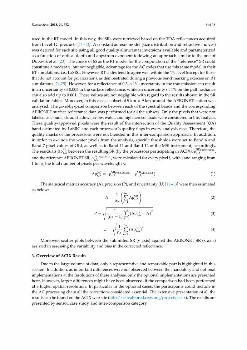
used in the RT model. In this way, the SRs were retrieved based on the TOA reflectances acquiredfrom Level-1C products [11–13]. A constant aerosol model (size distribution and refractive indices)was derived for each site using all good quality almucantar inversions available and parameterizedas a function of optical depth and angstrom exponent following an approach similar to the one ofDubovik et al. [23]. The choice of 6S as the RT model for the computation of the “reference” SR couldconstitute a moderate, but not negligible, advantage for the AC codes that use this same model in theirRT simulations, i.e., LaSRC. However, RT codes tend to agree well within the 1% level (except for thosethat do not account for polarization), as demonstrated during a previous benchmarking exercise on RTsimulations [24,25]. However, for a reflectance of 0.3, a 1% uncertainty in the transmission can resultin an uncertainty of 0.003 in the surface reflectance, while an uncertainty of 1% on the path radiancecan also add up to 0.001. These values are not negligible with regard to the results shown in the SRvalidation tables. Moreover, in this case, a subset of 9 km × 9 km around the AERONET station wasanalysed. The pixel-by-pixel comparison between each of the spectral bands and the correspondingAERONET surface reflectance data was performed for all the subsets. Only the pixels that were notlabeled as clouds, cloud shadows, snow, water, and high aerosol loads were considered in this analysis.These quality-approved pixels were the result of the intersection of the Quality Assessment (QA)band estimated by LaSRC and each processor’s quality flags in every analysis case. Therefore, thequality masks of the processors were not blended in this inter-comparison approach. In addition,in order to exclude the water pixels from the analysis, specific thresholds were set to Band 6 andBand 7 pixel values of OLI, as well as to Band 11 and Band 12 of the MSI instrument, accordingly.The residuals ∆ρSR
ι,λ between the resulting SR (by the processors participating in ACIX), ρSRPROCESSORι,λ ,
and the reference AERONET SR, ρSR AERONETι,λ , were calculated for every pixel i, with i and ranging from
1 to nλ the total number of pixels per wavelength λ:
∆ρSRι,λ = (ρSRPROCESSOR
ι,λ − ρSRAERONETι,λ ) (1)
The statistical metrics accuracy (A), precision (P), and uncertainty (U) [11–13] were then estimatedas below:
A =1
nλ
(nλ
∑i=1
∆ρSRι,λ
)(2)
P =
√1
(nλ − 1)
nλ
∑i=1
(∆ρSRι,λ − A)
2(3)
U =
√1
nλ
nλ
∑i=1
(∆ρSRι,λ)
2(4)
Moreover, scatter plots between the submitted SR (y axis) against the AERONET SR (x axis)assisted in assessing the variability and bias in the corrected reflectance.
3. Overview of ACIX Results
Due to the large volume of data, only a representative and remarkable part is highlighted in thissection. In addition, as important differences were not observed between the mandatory and optionalimplementations at the resolutions of these analyses, only the optional implementations are presentedhere. However, larger differences might have been observed, if the comparison had been performedat a higher spatial resolution. In particular in the optional cases, the participants could include inthe AC processing chain all the corrections considered essential. The extensive presentation of all theresults can be found on the ACIX web site (http://calvalportal.ceos.org/projects/acix). The results arepresented by sensor, case study, and inter-comparison category.
Remote Sens. 2018, 10, 352 7 of 18
3.1. Landsat-8
In total, four AC processors, i.e., ATCOR, FORCE, iCOR, and LaSRC, were applied to most of theL-8 datasets. GA-PABT was only implemented on the Australian site (Canberra), while ACOLITE andSeaDAS only for the coastal sites. Because of the small sample size of these cases, the interpretation ofthe inter-comparison results may be biased; therefore, the corresponding analyses are not presentedin this paper. These results, however, can be found on the ACIX web site. The data involved in theAOT analysis were filtered from (i) cloud; (ii) cloud shadow; (iii) adjacent to cloud; (iv) cirrus cloud;(v) no data values; and (vi) interpolated values. All the quality masks provided by the participantswere taken into consideration and a combined mask was used to exclude the unwanted pixels.
3.1.1. Aerosol Optical Thickness
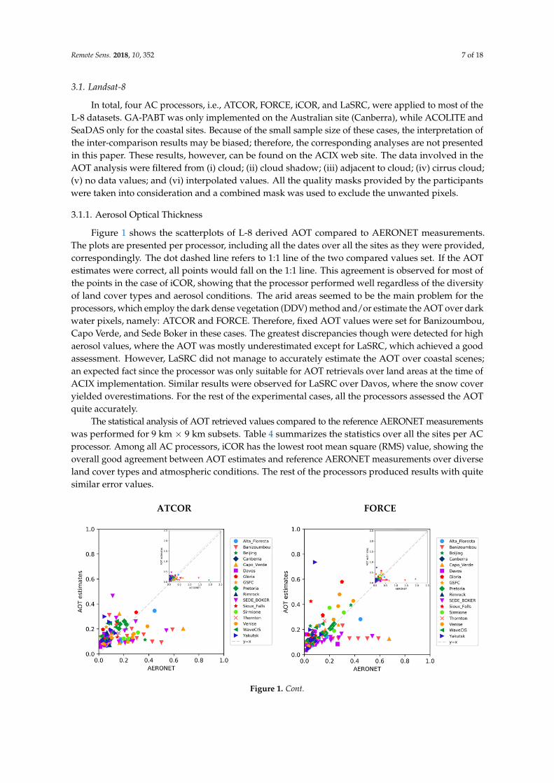
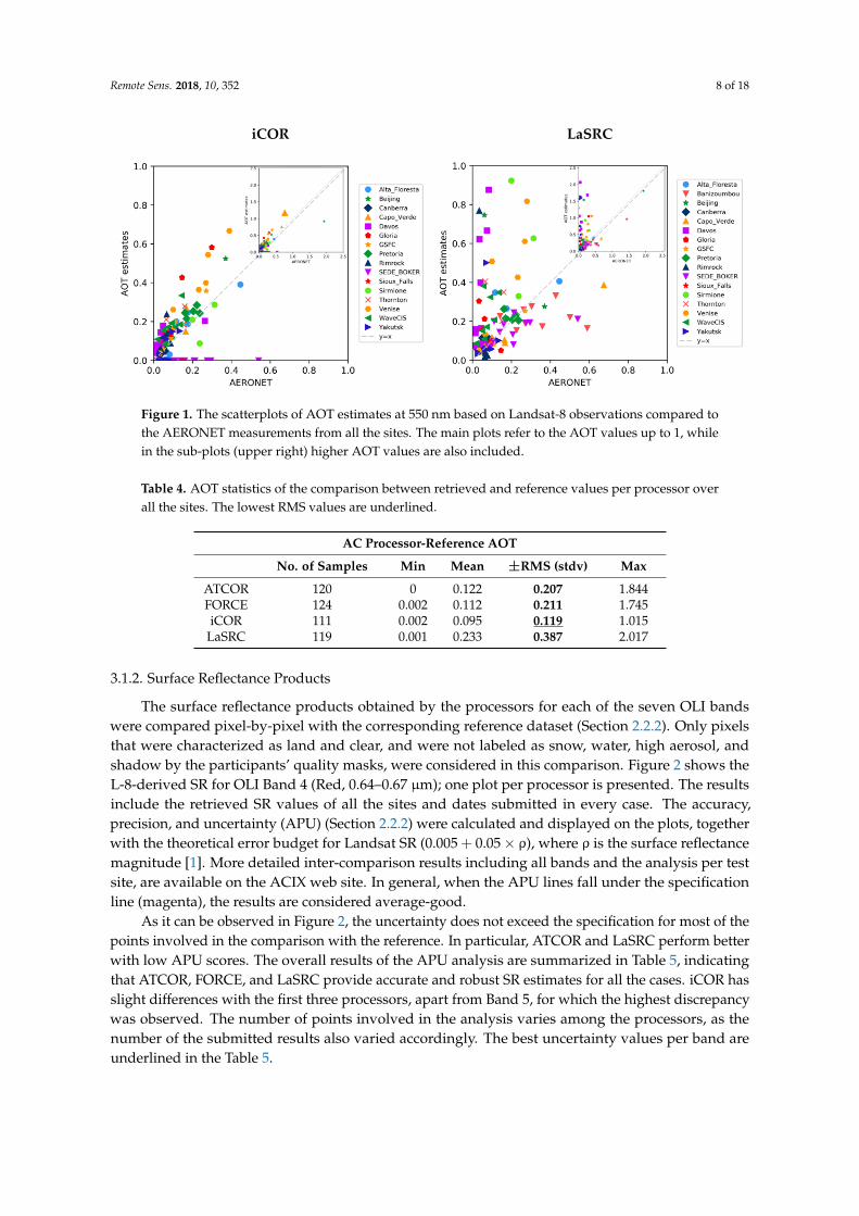
Figure 1 shows the scatterplots of L-8 derived AOT compared to AERONET measurements.The plots are presented per processor, including all the dates over all the sites as they were provided,correspondingly. The dot dashed line refers to 1:1 line of the two compared values set. If the AOTestimates were correct, all points would fall on the 1:1 line. This agreement is observed for most ofthe points in the case of iCOR, showing that the processor performed well regardless of the diversityof land cover types and aerosol conditions. The arid areas seemed to be the main problem for theprocessors, which employ the dark dense vegetation (DDV) method and/or estimate the AOT over darkwater pixels, namely: ATCOR and FORCE. Therefore, fixed AOT values were set for Banizoumbou,Capo Verde, and Sede Boker in these cases. The greatest discrepancies though were detected for highaerosol values, where the AOT was mostly underestimated except for LaSRC, which achieved a goodassessment. However, LaSRC did not manage to accurately estimate the AOT over coastal scenes;an expected fact since the processor was only suitable for AOT retrievals over land areas at the time ofACIX implementation. Similar results were observed for LaSRC over Davos, where the snow coveryielded overestimations. For the rest of the experimental cases, all the processors assessed the AOTquite accurately.
The statistical analysis of AOT retrieved values compared to the reference AERONET measurementswas performed for 9 km × 9 km subsets. Table 4 summarizes the statistics over all the sites per ACprocessor. Among all AC processors, iCOR has the lowest root mean square (RMS) value, showing theoverall good agreement between AOT estimates and reference AERONET measurements over diverseland cover types and atmospheric conditions. The rest of the processors produced results with quitesimilar error values.
Remote Sens. 2018, 10, x FOR PEER REVIEW 7 of 18
the participants were taken into consideration and a combined mask was used to exclude the unwanted pixels.
3.1.1. Aerosol Optical Thickness
Figure 1 shows the scatterplots of L-8 derived AOT compared to AERONET measurements. The plots are presented per processor, including all the dates over all the sites as they were provided, correspondingly. The dot dashed line refers to 1:1 line of the two compared values set. If the AOT estimates were correct, all points would fall on the 1:1 line. This agreement is observed for most of the points in the case of iCOR, showing that the processor performed well regardless of the diversity of land cover types and aerosol conditions. The arid areas seemed to be the main problem for the processors, which employ the dark dense vegetation (DDV) method and/or estimate the AOT over dark water pixels, namely: ATCOR and FORCE. Therefore, fixed AOT values were set for Banizoumbou, Capo Verde, and Sede Boker in these cases. The greatest discrepancies though were detected for high aerosol values, where the AOT was mostly underestimated except for LaSRC, which achieved a good assessment. However, LaSRC did not manage to accurately estimate the AOT over coastal scenes; an expected fact since the processor was only suitable for AOT retrievals over land areas at the time of ACIX implementation. Similar results were observed for LaSRC over Davos, where the snow cover yielded overestimations. For the rest of the experimental cases, all the processors assessed the AOT quite accurately.
ATCOR FORCE
iCOR LaSRC
Figure 1. The scatterplots of AOT estimates at 550 nm based on Landsat-8 observations compared to the AERONET measurements from all the sites. The main plots refer to the AOT values up to 1, while in the sub-plots (upper right) higher AOT values are also included.
Figure 1. Cont.
Remote Sens. 2018, 10, 352 8 of 18
Remote Sens. 2018, 10, x FOR PEER REVIEW 7 of 18
the participants were taken into consideration and a combined mask was used to exclude the unwanted pixels.
3.1.1. Aerosol Optical Thickness
Figure 1 shows the scatterplots of L-8 derived AOT compared to AERONET measurements. The plots are presented per processor, including all the dates over all the sites as they were provided, correspondingly. The dot dashed line refers to 1:1 line of the two compared values set. If the AOT estimates were correct, all points would fall on the 1:1 line. This agreement is observed for most of the points in the case of iCOR, showing that the processor performed well regardless of the diversity of land cover types and aerosol conditions. The arid areas seemed to be the main problem for the processors, which employ the dark dense vegetation (DDV) method and/or estimate the AOT over dark water pixels, namely: ATCOR and FORCE. Therefore, fixed AOT values were set for Banizoumbou, Capo Verde, and Sede Boker in these cases. The greatest discrepancies though were detected for high aerosol values, where the AOT was mostly underestimated except for LaSRC, which achieved a good assessment. However, LaSRC did not manage to accurately estimate the AOT over coastal scenes; an expected fact since the processor was only suitable for AOT retrievals over land areas at the time of ACIX implementation. Similar results were observed for LaSRC over Davos, where the snow cover yielded overestimations. For the rest of the experimental cases, all the processors assessed the AOT quite accurately.
ATCOR FORCE
iCOR LaSRC
Figure 1. The scatterplots of AOT estimates at 550 nm based on Landsat-8 observations compared to the AERONET measurements from all the sites. The main plots refer to the AOT values up to 1, while in the sub-plots (upper right) higher AOT values are also included.
Figure 1. The scatterplots of AOT estimates at 550 nm based on Landsat-8 observations compared tothe AERONET measurements from all the sites. The main plots refer to the AOT values up to 1, whilein the sub-plots (upper right) higher AOT values are also included.
Table 4. AOT statistics of the comparison between retrieved and reference values per processor overall the sites. The lowest RMS values are underlined.
AC Processor-Reference AOT
No. of Samples Min Mean ±RMS (stdv) Max
ATCOR 120 0 0.122 0.207 1.844FORCE 124 0.002 0.112 0.211 1.745iCOR 111 0.002 0.095 0.119 1.015
LaSRC 119 0.001 0.233 0.387 2.017
3.1.2. Surface Reflectance Products
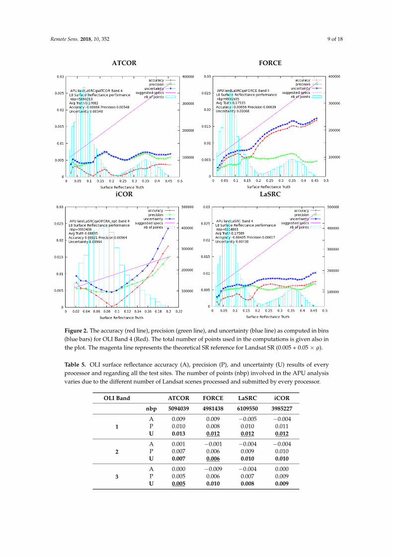
The surface reflectance products obtained by the processors for each of the seven OLI bandswere compared pixel-by-pixel with the corresponding reference dataset (Section 2.2.2). Only pixelsthat were characterized as land and clear, and were not labeled as snow, water, high aerosol, andshadow by the participants’ quality masks, were considered in this comparison. Figure 2 shows theL-8-derived SR for OLI Band 4 (Red, 0.64–0.67 µm); one plot per processor is presented. The resultsinclude the retrieved SR values of all the sites and dates submitted in every case. The accuracy,precision, and uncertainty (APU) (Section 2.2.2) were calculated and displayed on the plots, togetherwith the theoretical error budget for Landsat SR (0.005 + 0.05 × ρ), where ρ is the surface reflectancemagnitude [1]. More detailed inter-comparison results including all bands and the analysis per testsite, are available on the ACIX web site. In general, when the APU lines fall under the specificationline (magenta), the results are considered average-good.
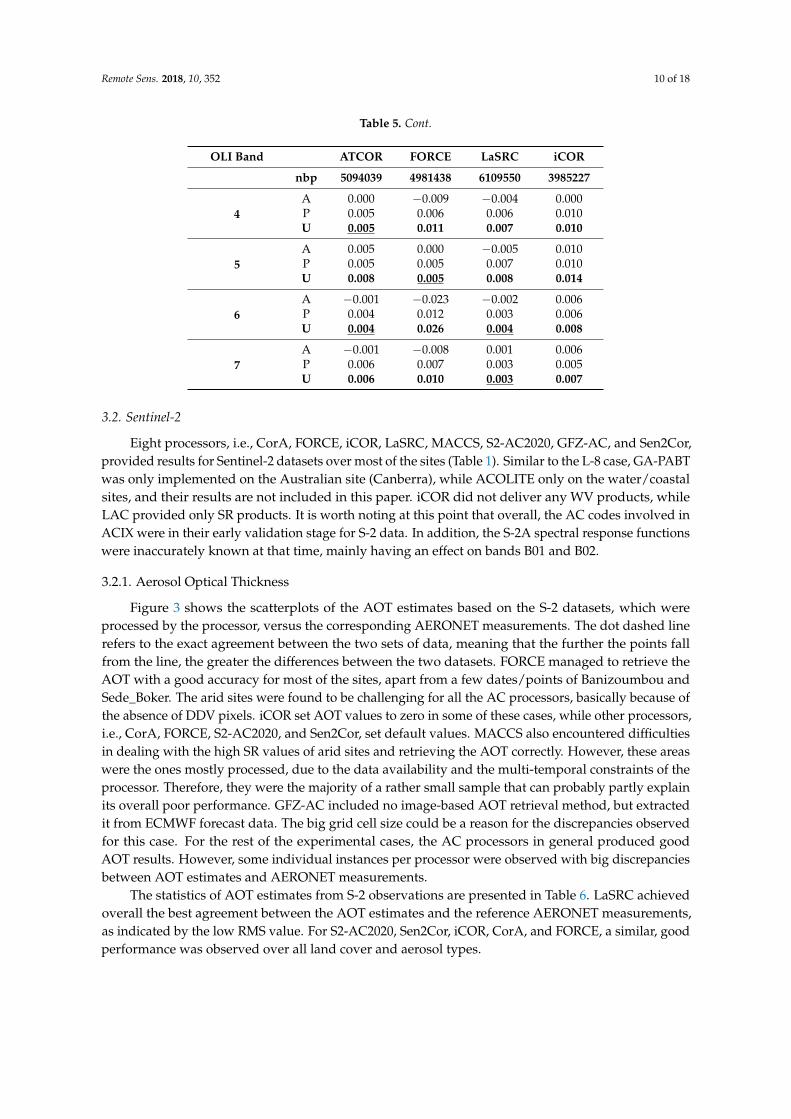
As it can be observed in Figure 2, the uncertainty does not exceed the specification for most of thepoints involved in the comparison with the reference. In particular, ATCOR and LaSRC perform betterwith low APU scores. The overall results of the APU analysis are summarized in Table 5, indicatingthat ATCOR, FORCE, and LaSRC provide accurate and robust SR estimates for all the cases. iCOR hasslight differences with the first three processors, apart from Band 5, for which the highest discrepancywas observed. The number of points involved in the analysis varies among the processors, as thenumber of the submitted results also varied accordingly. The best uncertainty values per band areunderlined in the Table 5.
Remote Sens. 2018, 10, 352 9 of 18
Remote Sens. 2018, 10, x FOR PEER REVIEW 8 of 18
The statistical analysis of AOT retrieved values compared to the reference AERONET measurements was performed for 9 km × 9 km subsets. Table 4 summarizes the statistics over all the sites per AC processor. Among all AC processors, iCOR has the lowest root mean square (RMS) value, showing the overall good agreement between AOT estimates and reference AERONET measurements over diverse land cover types and atmospheric conditions. The rest of the processors produced results with quite similar error values.
Table 4. AOT statistics of the comparison between retrieved and reference values per processor over all the sites. The lowest RMS values are underlined.
AC Processor-Reference AOT No. of Samples Min Mean ±RMS (stdv) Max
ATCOR 120 0 0.122 0.207 1.844 FORCE 124 0.002 0.112 0.211 1.745 iCOR 111 0.002 0.095 0.119 1.015
LaSRC 119 0.001 0.233 0.387 2.017
3.1.2. Surface Reflectance Products
The surface reflectance products obtained by the processors for each of the seven OLI bands were compared pixel-by-pixel with the corresponding reference dataset (Section 2.2.2). Only pixels that were characterized as land and clear, and were not labeled as snow, water, high aerosol, and shadow by the participants’ quality masks, were considered in this comparison. Figure 2 shows the L-8-derived SR for OLI Band 4 (Red, 0.64–0.67 µm); one plot per processor is presented. The results include the retrieved SR values of all the sites and dates submitted in every case. The accuracy, precision, and uncertainty (APU) (Section 2.2.2) were calculated and displayed on the plots, together with the theoretical error budget for Landsat SR (0.005 0.05 ρ), where ρ is the surface reflectance magnitude [1]. More detailed inter-comparison results including all bands and the analysis per test site, are available on the ACIX web site. In general, when the APU lines fall under the specification line (magenta), the results are considered average-good.
ATCOR FORCE
iCOR LaSRC Remote Sens. 2018, 10, x FOR PEER REVIEW 9 of 18
Figure 2. The accuracy (red line), precision (green line), and uncertainty (blue line) as computed in bins (blue bars) for OLI Band 4 (Red). The total number of points used in the computations is given also in the plot. The magenta line represents the theoretical SR reference for Landsat SR (0.005 + 0.05 × ρ).
As it can be observed in Figure 2, the uncertainty does not exceed the specification for most of the points involved in the comparison with the reference. In particular, ATCOR and LaSRC perform better with low APU scores. The overall results of the APU analysis are summarized in Table 5, indicating that ATCOR, FORCE, and LaSRC provide accurate and robust SR estimates for all the cases. iCOR has slight differences with the first three processors, apart from Band 5, for which the highest discrepancy was observed. The number of points involved in the analysis varies among the processors, as the number of the submitted results also varied accordingly. The best uncertainty values per band are underlined in the Table 5.
Table 5. OLI surface reflectance accuracy (A), precision (P), and uncertainty (U) results of every processor and regarding all the test sites. The number of points (nbp) involved in the APU analysis varies due to the different number of Landsat scenes processed and submitted by every processor.
OLI Band ATCOR FORCE LaSRC iCOR nbp 5094039 4981438 6109550 3985227
1 A 0.009 0.009 −0.005 −0.004 P 0.010 0.008 0.010 0.011 U 0.013 0.012 0.012 0.012
2 A 0.001 −0.001 −0.004 −0.004 P 0.007 0.006 0.009 0.010 U 0.007 0.006 0.010 0.010
3 A 0.000 −0.009 −0.004 0.000 P 0.005 0.006 0.007 0.009 U 0.005 0.010 0.008 0.009
4 A 0.000 −0.009 −0.004 0.000 P 0.005 0.006 0.006 0.010 U 0.005 0.011 0.007 0.010
5 A 0.005 0.000 −0.005 0.010 P 0.005 0.005 0.007 0.010 U 0.008 0.005 0.008 0.014
6 A −0.001 −0.023 −0.002 0.006 P 0.004 0.012 0.003 0.006 U 0.004 0.026 0.004 0.008
7 A −0.001 −0.008 0.001 0.006 P 0.006 0.007 0.003 0.005 U 0.006 0.010 0.003 0.007
Figure 2. The accuracy (red line), precision (green line), and uncertainty (blue line) as computed in bins(blue bars) for OLI Band 4 (Red). The total number of points used in the computations is given also inthe plot. The magenta line represents the theoretical SR reference for Landsat SR (0.005 + 0.05 × ρ).
Table 5. OLI surface reflectance accuracy (A), precision (P), and uncertainty (U) results of everyprocessor and regarding all the test sites. The number of points (nbp) involved in the APU analysisvaries due to the different number of Landsat scenes processed and submitted by every processor.
OLI Band ATCOR FORCE LaSRC iCOR
nbp 5094039 4981438 6109550 3985227
1A 0.009 0.009 −0.005 −0.004P 0.010 0.008 0.010 0.011U 0.013 0.012 0.012 0.012
2A 0.001 −0.001 −0.004 −0.004P 0.007 0.006 0.009 0.010U 0.007 0.006 0.010 0.010
3A 0.000 −0.009 −0.004 0.000P 0.005 0.006 0.007 0.009U 0.005 0.010 0.008 0.009
Remote Sens. 2018, 10, 352 10 of 18
Table 5. Cont.
OLI Band ATCOR FORCE LaSRC iCOR
nbp 5094039 4981438 6109550 3985227
4A 0.000 −0.009 −0.004 0.000P 0.005 0.006 0.006 0.010U 0.005 0.011 0.007 0.010
5A 0.005 0.000 −0.005 0.010P 0.005 0.005 0.007 0.010U 0.008 0.005 0.008 0.014
6A −0.001 −0.023 −0.002 0.006P 0.004 0.012 0.003 0.006U 0.004 0.026 0.004 0.008
7A −0.001 −0.008 0.001 0.006P 0.006 0.007 0.003 0.005U 0.006 0.010 0.003 0.007
3.2. Sentinel-2
Eight processors, i.e., CorA, FORCE, iCOR, LaSRC, MACCS, S2-AC2020, GFZ-AC, and Sen2Cor,provided results for Sentinel-2 datasets over most of the sites (Table 1). Similar to the L-8 case, GA-PABTwas only implemented on the Australian site (Canberra), while ACOLITE only on the water/coastalsites, and their results are not included in this paper. iCOR did not deliver any WV products, whileLAC provided only SR products. It is worth noting at this point that overall, the AC codes involved inACIX were in their early validation stage for S-2 data. In addition, the S-2A spectral response functionswere inaccurately known at that time, mainly having an effect on bands B01 and B02.
3.2.1. Aerosol Optical Thickness
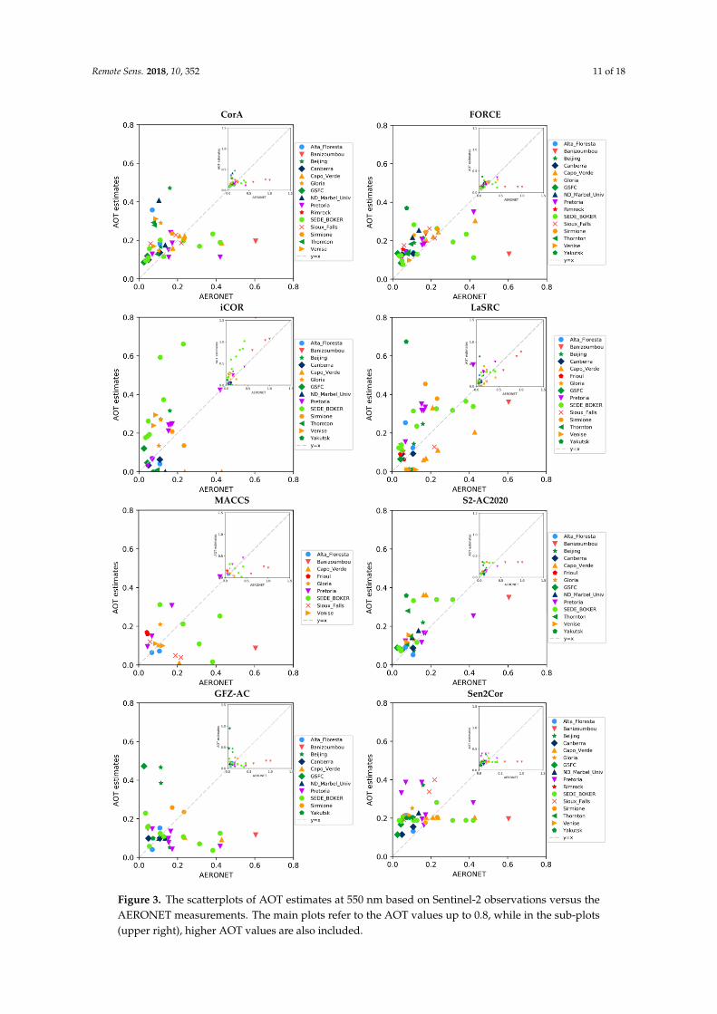
Figure 3 shows the scatterplots of the AOT estimates based on the S-2 datasets, which wereprocessed by the processor, versus the corresponding AERONET measurements. The dot dashed linerefers to the exact agreement between the two sets of data, meaning that the further the points fallfrom the line, the greater the differences between the two datasets. FORCE managed to retrieve theAOT with a good accuracy for most of the sites, apart from a few dates/points of Banizoumbou andSede_Boker. The arid sites were found to be challenging for all the AC processors, basically because ofthe absence of DDV pixels. iCOR set AOT values to zero in some of these cases, while other processors,i.e., CorA, FORCE, S2-AC2020, and Sen2Cor, set default values. MACCS also encountered difficultiesin dealing with the high SR values of arid sites and retrieving the AOT correctly. However, these areaswere the ones mostly processed, due to the data availability and the multi-temporal constraints of theprocessor. Therefore, they were the majority of a rather small sample that can probably partly explainits overall poor performance. GFZ-AC included no image-based AOT retrieval method, but extractedit from ECMWF forecast data. The big grid cell size could be a reason for the discrepancies observedfor this case. For the rest of the experimental cases, the AC processors in general produced goodAOT results. However, some individual instances per processor were observed with big discrepanciesbetween AOT estimates and AERONET measurements.
The statistics of AOT estimates from S-2 observations are presented in Table 6. LaSRC achievedoverall the best agreement between the AOT estimates and the reference AERONET measurements,as indicated by the low RMS value. For S2-AC2020, Sen2Cor, iCOR, CorA, and FORCE, a similar, goodperformance was observed over all land cover and aerosol types.
Remote Sens. 2018, 10, 352 11 of 18
Remote Sens. 2018, 10, x FOR PEER REVIEW 11 of 18
CorA FORCE
iCOR LaSRC
MACCS S2-AC2020
GFZ-AC Sen2Cor
Figure 3. The scatterplots of AOT estimates at 550 nm based on Sentinel-2 observations versus the AERONET measurements. The main plots refer to the AOT values up to 0.8, while in the sub-plots (upper right), higher AOT values are also included.
Figure 3. The scatterplots of AOT estimates at 550 nm based on Sentinel-2 observations versus theAERONET measurements. The main plots refer to the AOT values up to 0.8, while in the sub-plots(upper right), higher AOT values are also included.
Remote Sens. 2018, 10, 352 12 of 18
Table 6. AOT statistics of the comparison between retrieved and reference values per processor overall the sites. The lowest RMS values are underlined.
AC Processor-Reference AOT
No. of Samples Min Mean ±RMS (Stdv) Max
CorA 47 0 0.133 0.155 0.757FORCE 48 0.003 0.116 0.169 0.871iCOR 37 0.002 0.15 0.151 0.599
LaSRC 48 0.002 0.115 0.097 0.602MACCS 24 0.002 0.176 0.2 0.778
S2-AC2020 36 0.002 0.107 0.144 0.652GFZ-AC 41 0.001 0.159 0.223 0.92Sen2Cor 47 0.005 0.158 0.147 0.805
3.2.2. Water Vapour (WV)
Water Vapour was an additional product derived from S-2 observations. Seven processors includedthe WV estimation in their approaches, i.e., CorA, FORCE, LaSRC, MACCS, S2-AC2020, GFZ-AC, andSen2Cor. The inter-comparison analysis was similar to the one implemented to inter-compare the AOTvalues. It should be noted that the pixels labeled as ‘Water’ in the participants’ quality masks wereexcluded from the analysis of WV retrievals.
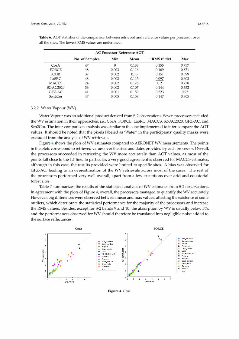
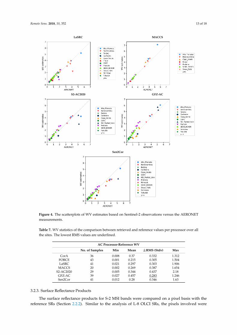
Figure 4 shows the plots of WV estimates compared to AERONET WV measurements. The pointsin the plots correspond to retrieved values over the sites and dates provided by each processor. Overall,the processors succeeded in retrieving the WV more accurately than AOT values, as most of thepoints fall close to the 1:1 line. In particular, a very good agreement is observed for MACCS estimates,although in this case, the results provided were limited to specific sites. A bias was observed forGFZ-AC, leading to an overestimation of the WV retrievals across most of the cases. The rest ofthe processors performed very well overall, apart from a few exceptions over arid and equatorialforest sites.
Table 7 summarizes the results of the statistical analysis of WV estimates from S-2 observations.In agreement with the plots of Figure 4, overall, the processors managed to quantify the WV accurately.However, big differences were observed between mean and max values, attesting the existence of someoutliers, which deteriorate the statistical performance for the majority of the processors and increasethe RMS values. Besides, except for S-2 bands 9 and 10, the absorption by WV is usually below 5%,and the performances observed for WV should therefore be translated into negligible noise added tothe surface reflectances.
Remote Sens. 2018, 10, x FOR PEER REVIEW 12 of 18
3.2.2. Water Vapour (WV)
Water Vapour was an additional product derived from S-2 observations. Seven processors included the WV estimation in their approaches, i.e., CorA, FORCE, LaSRC, MACCS, S2-AC2020, GFZ-AC, and Sen2Cor. The inter-comparison analysis was similar to the one implemented to inter-compare the AOT values. It should be noted that the pixels labeled as ‘Water’ in the participants’ quality masks were excluded from the analysis of WV retrievals.
Figure 4 shows the plots of WV estimates compared to AERONET WV measurements. The points in the plots correspond to retrieved values over the sites and dates provided by each processor. Overall, the processors succeeded in retrieving the WV more accurately than AOT values, as most of the points fall close to the 1:1 line. In particular, a very good agreement is observed for MACCS estimates, although in this case, the results provided were limited to specific sites. A bias was observed for GFZ-AC, leading to an overestimation of the WV retrievals across most of the cases. The rest of the processors performed very well overall, apart from a few exceptions over arid and equatorial forest sites.
Table 7 summarizes the results of the statistical analysis of WV estimates from S-2 observations. In agreement with the plots of Figure 4, overall, the processors managed to quantify the WV accurately. However, big differences were observed between mean and max values, attesting the existence of some outliers, which deteriorate the statistical performance for the majority of the processors and increase the RMS values. Besides, except for S-2 bands 9 and 10, the absorption by WV is usually below 5%, and the performances observed for WV should therefore be translated into negligible noise added to the surface reflectances.
Table 7. WV statistics of the comparison between retrieved and reference values per processor over all the sites. The lowest RMS values are underlined.
AC Processor-Reference WV No. of Samples Min Mean ±RMS (Stdv) Max
CorA 36 0.008 0.37 0.332 1.312 FORCE 43 0.001 0.215 0.305 1.504 LaSRC 41 0.021 0.297 0.303 1.906
MACCS 20 0.002 0.269 0.387 1.654 S2-AC2020 29 0.005 0.344 0.437 2.18
GFZ-AC 39 0.027 0.457 0.283 1.246 Sen2Cor 41 0.012 0.28 0.346 1.63
CorA FORCE
Figure 4. Cont.
Remote Sens. 2018, 10, 352 13 of 18
Remote Sens. 2018, 10, x FOR PEER REVIEW 13 of 18
LaSRC MACCS
S2-AC2020 GFZ-AC
Sen2Cor
Figure 4. The scatterplots of WV estimates based on Sentinel-2 observations versus the AERONET measurements.
3.2.3. Surface Reflectance Products
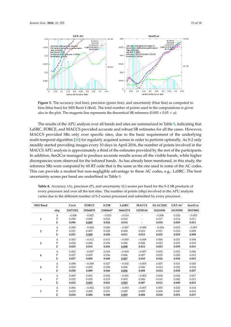
The surface reflectance products for S-2 MSI bands were compared on a pixel basis with the reference SRs (Section 2.2.2). Similar to the analysis of L-8 OLCI SRs, the pixels involved were labeled as land and clear, and were filtered from snow, water, high aerosol, and shadow based on the participants’ quality masks. As has already been mentioned, the APU analysis of all the SR values obtained by every processor and for every site is available on the ACIX web site. Band 9 (Water vapour) and Band 10 (SWIR–Cirrus) were excluded from this analysis because they are not intended for land applications. Figure 5 demonstrates a representative example of the APU outcomes for MSI Band 4 (Red, central wavelength 665 nm) for all the datasets processed by the processor. The overall analysis of the plots shows that FORCE, LaSRC, MACCS, and Sen2Cor managed to estimate the SRs quite well over all the sites. The good performance is confirmed by the low values of accuracy (A), proving that the SR products are not biased. In addition, U curves fall under the line of specified uncertainty, showing that these processors met the requirement of the theoretical SR reference [1].
Figure 4. The scatterplots of WV estimates based on Sentinel-2 observations versus the AERONETmeasurements.
Table 7. WV statistics of the comparison between retrieved and reference values per processor over allthe sites. The lowest RMS values are underlined.
AC Processor-Reference WV
No. of Samples Min Mean ±RMS (Stdv) Max
CorA 36 0.008 0.37 0.332 1.312FORCE 43 0.001 0.215 0.305 1.504LaSRC 41 0.021 0.297 0.303 1.906
MACCS 20 0.002 0.269 0.387 1.654S2-AC2020 29 0.005 0.344 0.437 2.18
GFZ-AC 39 0.027 0.457 0.283 1.246Sen2Cor 41 0.012 0.28 0.346 1.63
3.2.3. Surface Reflectance Products
The surface reflectance products for S-2 MSI bands were compared on a pixel basis with thereference SRs (Section 2.2.2). Similar to the analysis of L-8 OLCI SRs, the pixels involved were

Remote Sens. 2018, 10, 352 14 of 18
labeled as land and clear, and were filtered from snow, water, high aerosol, and shadow based on theparticipants’ quality masks. As has already been mentioned, the APU analysis of all the SR valuesobtained by every processor and for every site is available on the ACIX web site. Band 9 (Water vapour)and Band 10 (SWIR–Cirrus) were excluded from this analysis because they are not intended for landapplications. Figure 5 demonstrates a representative example of the APU outcomes for MSI Band 4(Red, central wavelength 665 nm) for all the datasets processed by the processor. The overall analysisof the plots shows that FORCE, LaSRC, MACCS, and Sen2Cor managed to estimate the SRs quitewell over all the sites. The good performance is confirmed by the low values of accuracy (A), provingthat the SR products are not biased. In addition, U curves fall under the line of specified uncertainty,showing that these processors met the requirement of the theoretical SR reference [1].
Remote Sens. 2018, 10, x FOR PEER REVIEW 15 of 18
CorA FORCE
iCOR LaSRC
MACCS S2-AC2020
Figure 5. Cont.
Remote Sens. 2018, 10, 352 15 of 18
Remote Sens. 2018, 10, x FOR PEER REVIEW 16 of 18
GFZ-AC Sen2Cor
Figure 5. The accuracy (red line), precision (green line), and uncertainty (blue line) as computed in bins (blue bars) for MSI Band 4 (Red). The total number of points used in the computations is given also in the plot. The magenta line represents the theoretical SR reference (0.005 + 0.05 × ρ).
4. Conclusions
The ACIX is designed as an open and free initiative to compare AC codes applicable either to L-8 or S-2 imagery. Therefore, every developer of an AC algorithm was welcome to participate in the exercise. Indeed, in the first implementation of ACIX, several participants from different institutes, companies, and agencies around the world contributed by defining the inter-comparison protocol and processing a big volume of data. However, different factors, e.g., time constraints, tuning of the processors, processor’s limitations, etc., prevented the application of some AC algorithms to the whole L-8 and/or S-2 dataset. Due to this variance of the submitted results, it was not feasible to draw common conclusions among all the algorithms, but fortunately, these cases were not the majority. Being completed for the first time, ACIX has proven to be successful in (a) addressing the strengths and weaknesses of the processors over diverse land cover types and atmospheric conditions, (b) quantifying the discrepancies of AOT and WV products compared to AERONET measurements, and (c) identifying the similarities among the processors by analysing and presenting all the results in the same manner.
The ACIX results are a unique source of information over the performance of notable AC processors, which will be made publicly available on the CEOS Cal/Val portal. Based on these outcomes, the user and scientific community can be informed about the state-of-art approaches, including their highlights and shortcomings, across different sensors, products, and sites. It should be noted here that the developers were determined to participate in the exercise; although the processors were not mature enough to handle different source data and land cover types. Considering S-2 datasets for instance, ACIX only started six months after the beginning of S-2 Level-1 data provision to all users. The research community was still inexperienced during that phase, and time and effort was needed to adapt the processors to the new data requirements. The discrepancies observed in ACIX inter-comparison results have assisted, in many cases, the developers to learn about the performance and identify the flaws in their algorithms. As a matter of fact, the participants have already modified and improved their processors and will have a chance to present the enhanced versions during the following ACIX implementation.
The continuation of the exercise has already been discussed and agreed, suggesting some new implementation parameters. More datasets need to be exploited, in order to obtain more concrete conclusions, so at least a one-year period of complete time series from L-8, S-2A, and S-2B will be employed. However, it is important that all the participants will apply their processors over all sites, in order to gain an overall assessment of their inter-performance. The sites will also be redefined and more representative cases concerning land cover and aerosol types will be included. The analyses of the performances over aquatic sites (i.e., coastal and inland waters) and comparisons of cloud masks
Figure 5. The accuracy (red line), precision (green line), and uncertainty (blue line) as computed inbins (blue bars) for MSI Band 4 (Red). The total number of points used in the computations is givenalso in the plot. The magenta line represents the theoretical SR reference (0.005 + 0.05 × ρ).
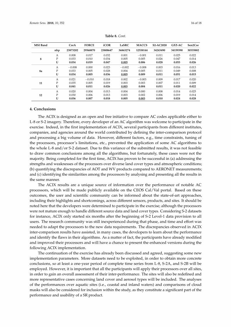
The results of the APU analysis over all bands and sites are summarized in Table 8, indicating thatLaSRC, FORCE, and MACCS provided accurate and robust SR estimates for all the cases. However,MACCS provided SRs only over specific sites, due to the basic requirement of the underlyingmulti-temporal algorithm [26] for regularly acquired scenes in order to perform optimally. As S-2 onlysteadily started providing images every 10 days in April 2016, the number of points involved in theMACCS APU analysis is approximately a third of the estimates provided by the rest of the participants.In addition, Sen2Cor managed to produce accurate results across all the visible bands, while higherdiscrepancies were observed for the infrared bands. As has already been mentioned, in this study, thereference SRs were computed by 6S RT code that is the same as the one used in some of the AC codes.This can provide a modest but non-negligible advantage to these AC codes, e.g., LaSRC. The bestuncertainty scores per band are underlined in Table 8.
Table 8. Accuracy (A), precision (P), and uncertainty (U) scores per band for the S-2 SR products ofevery processor and over all the test sites. The number of points (nbp) involved in the APU analysisvaries due to the different number of S-2 scenes processed and submitted by every processor.
MSI Band CorA FORCE iCOR LaSRC MACCS S2-AC2020 GFZ-AC Sen2Cor
nbp 23873202 29568870 23808647 36863274 12538144 34243490 34159390 30335882
1A −0.006 −0.002 −0.010 −0.010 - −0.006 0.026 −0.003P 0.096 0.009 0.024 0.010 - 0.017 0.014 0.011U 0.096 0.009 0.026 0.014 - 0.018 0.029 0.011
2A 0.000 −0.004 0.000 −0.007 −0.008 −0.004 0.023 −0.001P 0.021 0.007 0.028 0.008 0.010 0.021 0.016 0.009U 0.021 0.008 0.028 0.011 0.013 0.022 0.029 0.009
3A 0.003 −0.012 0.013 −0.005 −0.008 0.000 0.031 0.004P 0.024 0.006 0.034 0.006 0.008 0.023 0.023 0.010U 0.025 0.014 0.036 0.008 0.012 0.023 0.039 0.011
4A 0.002 −0.007 0.018 −0.003 −0.007 0.002 0.022 0.006P 0.027 0.005 0.036 0.006 0.007 0.025 0.020 0.012U 0.027 0.009 0.040 0.007 0.010 0.026 0.030 0.013
5A 0.008 −0.008 0.027 −0.002 −0.005 0.007 0.031 0.020P 0.029 0.005 0.038 0.006 0.006 0.012 0.022 0.018U 0.030 0.009 0.046 0.006 0.008 0.014 0.038 0.027
6A 0.005 0.001 0.024 −0.001 −0.003 0.004 0.024 0.017P 0.032 0.005 0.033 0.005 0.006 0.010 0.042 0.011U 0.032 0.005 0.041 0.005 0.007 0.011 0.049 0.021
7A 0.006 −0.002 0.025 −0.003 −0.007 0.005 0.020 0.014P 0.033 0.005 0.031 0.005 0.005 0.009 0.047 0.010U 0.034 0.006 0.040 0.005 0.008 0.010 0.051 0.017
Remote Sens. 2018, 10, 352 16 of 18
Table 8. Cont.
MSI Band CorA FORCE iCOR LaSRC MACCS S2-AC2020 GFZ-AC Sen2Cor
nbp 23873202 29568870 23808647 36863274 12538144 34243490 34159390 30335882
8A 0.008 0.017 0.032 0.001 −0.001 0.011 0.025 0.022P 0.033 0.010 0.034 0.005 0.005 0.026 0.047 0.014U 0.034 0.019 0.047 0.005 0.006 0.028 0.053 0.026
8aA −0.008 0.000 0.023 −0.002 −0.008 0.003 0.016 0.013P 0.033 0.005 0.028 0.004 0.005 0.011 0.049 0.008U 0.034 0.005 0.036 0.005 0.009 0.011 0.051 0.015
11A 0.021 −0.010 0.018 0.002 −0.003 0.009 0.017 0.020P 0.035 0.005 0.019 0.003 0.003 0.007 0.011 0.009U 0.041 0.011 0.026 0.003 0.004 0.011 0.020 0.022
12A 0.020 0.004 0.013 0.004 0.000 0.008 0.014 0.025P 0.030 0.006 0.013 0.003 0.002 0.006 0.019 0.014U 0.036 0.007 0.018 0.005 0.003 0.010 0.024 0.028
4. Conclusions
The ACIX is designed as an open and free initiative to compare AC codes applicable either toL-8 or S-2 imagery. Therefore, every developer of an AC algorithm was welcome to participate in theexercise. Indeed, in the first implementation of ACIX, several participants from different institutes,companies, and agencies around the world contributed by defining the inter-comparison protocoland processing a big volume of data. However, different factors, e.g., time constraints, tuning ofthe processors, processor’s limitations, etc., prevented the application of some AC algorithms tothe whole L-8 and/or S-2 dataset. Due to this variance of the submitted results, it was not feasibleto draw common conclusions among all the algorithms, but fortunately, these cases were not themajority. Being completed for the first time, ACIX has proven to be successful in (a) addressing thestrengths and weaknesses of the processors over diverse land cover types and atmospheric conditions;(b) quantifying the discrepancies of AOT and WV products compared to AERONET measurements;and (c) identifying the similarities among the processors by analysing and presenting all the results inthe same manner.
The ACIX results are a unique source of information over the performance of notable ACprocessors, which will be made publicly available on the CEOS Cal/Val portal. Based on theseoutcomes, the user and scientific community can be informed about the state-of-art approaches,including their highlights and shortcomings, across different sensors, products, and sites. It should benoted here that the developers were determined to participate in the exercise; although the processorswere not mature enough to handle different source data and land cover types. Considering S-2 datasetsfor instance, ACIX only started six months after the beginning of S-2 Level-1 data provision to allusers. The research community was still inexperienced during that phase, and time and effort wasneeded to adapt the processors to the new data requirements. The discrepancies observed in ACIXinter-comparison results have assisted, in many cases, the developers to learn about the performanceand identify the flaws in their algorithms. As a matter of fact, the participants have already modifiedand improved their processors and will have a chance to present the enhanced versions during thefollowing ACIX implementation.
The continuation of the exercise has already been discussed and agreed, suggesting some newimplementation parameters. More datasets need to be exploited, in order to obtain more concreteconclusions, so at least a one-year period of complete time series from L-8, S-2A, and S-2B will beemployed. However, it is important that all the participants will apply their processors over all sites,in order to gain an overall assessment of their inter-performance. The sites will also be redefined andmore representative cases concerning land cover and aerosol types will be included. The analysesof the performances over aquatic sites (i.e., coastal and inland waters) and comparisons of cloudmasks will also be considered for inclusion within the study, as they constitute a significant part of theperformance and usability of a SR product.
Remote Sens. 2018, 10, 352 17 of 18
Having experience of the first ACIX implementation, the inter-comparison strategy will berefined, complementing the current metrics with comparisons to other sources of measurements,e.g., RadCalNet, and analysis at a higher spatial resolution (pixel scale) in order to allow testing theadjacency effect correction. Using criteria that assess the time consistency of time series would alsoprovide an idea of the noise that affects L2A time series, including the effects of undetected clouds orshadows. The next phase of ACIX is anticipated to involve more participants and more datasets willbe assessed.
Acknowledgments: The authors would like to thank all the AERONET Principal Investigators and their staff forestablishing and maintaining the 19 sites used in this investigation. We would like also to thank the editors andthe anonymous reviewers for their constructive comments, which helped us to improve the quality of the article.
Author Contributions: Georgia Doxani, Eric Vermote, Jean-Claude Roger and Ferran Gascon contributed to thedefinition of the protocol, the inter-comparison analysis and the preparation of the manuscript. Eric Vermote,Stefan Adriaensen David Frantz, Olivier Hagolle, André Hollstein, Grit Kirches, Fuqin Li, Jérôme Louis,Antoine Mangin, Nima Pahlevan, Bringfried Pflug and Quinten Vanhellmont contributed to the definitionof the protocol, implemented their AC processors on the input data and participated in the preparation ofthe manuscript.
Conflicts of Interest: The authors declare no conflict of interest.
References
1. Vermote, E.F.; Kotchenova, S. Atmospheric correction for the monitoring of land surfaces. J. Geophys. Res.2008, 113. [CrossRef]
2. Franch, B.; Vermote, E.F.; Roger, J.C.; Murphy, E.; Becker-Reshef, I.; Justice, C.; Claverie, M.; Nagol, J.;Csiszar, I.; Meyer, D.; et al. A 30+ Year AVHRR Land Surface Reflectance Climate Data Record and ItsApplication to Wheat Yield Monitoring. Remote Sens. 2017, 9, 296. [CrossRef]
3. Hagolle, O.; Huc, M.; Villa Pascual, D.; Dedieu, G. A multi-temporal and multi-spectral method to estimateaerosol optical thickness over land, for the atmospheric correction of FormoSat-2, LandSat, VENµS andSentinel-2 images. Remote Sens. 2015, 7, 2668–2691. [CrossRef]
4. Ng, W.T.; Rima, P.; Einzmann, K.; Immitzer, M.; Atzberger, C.; Eckert, S. Assessing the Potential of Sentinel-2and Pléiades Data for the Detection of Prosopis and Vachellia spp. in Kenya. Remote Sens. 2017, 9, 74.[CrossRef]
5. Van der Werff, H.; Van der Meer, F. Sentinel-2A MSI and Landsat 8 OLI Provide Data Continuity forGeological Remote Sensing. Remote Sens. 2016, 8, 883. [CrossRef]
6. Radoux, J.; Chomé, G.; Jacques, D.C.; Waldner, F.; Bellemans, N.; Matton, N.; Lamarche, C.; d’Andrimont, R.;Defourny, P. Sentinel-2’s Potential for Sub-Pixel Landscape Feature Detection. Remote Sens. 2016, 8, 488.[CrossRef]
7. Pahlevan, N.; Sarkar, S.; Franz, B.A.; Balasubramanian, S.V.; He, J. Sentinel-2 MultiSpectral Instrument (MSI)data processing for aquatic science applications: Demonstrations and validations. Remote Sens. Environ.2017, 201, 47–56. [CrossRef]
8. Pahlevan, N.; Schott, J.R.; Franz, B.A.; Zibordi, G.; Markham, B.; Bailey, S.; Schaaf, C.B.; Ondrusek, M.;Greb, S.; Strait, C.M. Landsat 8 remote sensing reflectance (R rs) products: Evaluations, intercomparisons,and enhancements. Remote Sens. Environ. 2017, 190, 289–301. [CrossRef]
9. Rouquié, B.; Hagolle, O.; Bréon, F.-M.; Boucher, O.; Desjardins, C.; Rémy, S. Using Copernicus AtmosphereMonitoring Service Products to Constrain the Aerosol Type in the Atmospheric Correction Processor MAJA.Remote Sens. 2017, 9, 1230. [CrossRef]
10. Dörnhöfer, K.; Göritz, A.; Gege, P.; Pflug, B.; Oppelt, N. Water Constituents and Water Depth Retrieval fromSentinel-2A—A First Evaluation in an Oligotrophic Lake. Remote Sens. 2016, 8, 941. [CrossRef]
11. Ju, J.; Roy, D.P.; Vermote, E.; Masek, J.; Kovalskyy, V. Continental-scale validation of MODIS-based andLEDAPS Landsat ETM+ atmospheric correction methods. Remote Sens. Environ. 2012, 122, 175–184. [CrossRef]
12. Claverie, M.; Vermote, E.F.; Franch, B.; Masek, J.G. Evaluation of the Landsat-5 TM and Landsat-7 ETM+surface reflectance products. Remote Sens. Environ. 2015, 169, 390–403. [CrossRef]
13. Vermote, E.; Justice, C.; Claverie, M.; Franch, B. Preliminary analysis of the performance of the Landsat8/OLI land surface reflectance product. Remote Sens. Environ. 2016, 185, 46–56. [CrossRef]
Remote Sens. 2018, 10, 352 18 of 18
14. Holben, B.N.; Eck, T.F.; Slutsker, I.; Tanre, D.; Buis, J.P.; Setzer, A.; Vermote, E.; Reagan, J.A.; Kaufman, Y.J.;Nakajima, T.; et al. AERONET—A federated instrument network and data archive for aerosol characterization.Remote Sens. Environ. 1998, 66, 1–16. [CrossRef]
15. Smirnov, A.; Holben, B.N.; Eck, T.F.; Dubovik, O.; Slutsker, I. Cloud-screening and quality control algorithmsfor the AERONET database. Remote Sens. Environ. 2000, 73, 337–349. [CrossRef]
16. Richter, R. Correction of satellite imagery over mountainous terrain. Appl. Opt. 1998, 37, 4004–4015.[CrossRef] [PubMed]
17. Richter, R.; Schläpfer, D. Atmospheric/Topographic Correction for Satellite Imagery; DLR Report DLR-IB565-02/15); German Aerospace Center (DLR): Wessling, Germany, 2015.
18. Defourny, P.; Arino, O.; Boettcher, M.; Brockmann, C.; Kirches, G.; Lamarche, C.; Radoux, J.; Ramoino, F.;Santoro, M.; Wevers, J. CCI-LC ATBDv3 Phase II. Land Cover Climate Change Initiative—AlgorithmTheoretical Basis Document v3. Issue 1.1, 2017. Available online: https://www.esa-landcover-cci.org/?q=documents# (accessed on 20 February 2018).
19. Frantz, D.; Röder, A.; Stellmes, M.; Hill, J. An Operational Radiometric Landsat Preprocessing Frameworkfor Large-Area Time Series Applications. IEEE Trans. Geosci. Remote Sens. 2016, 54, 3928–3943. [CrossRef]
20. Li, F.; Jupp, D.L.B.; Thankappan, M.; Lymburner, L.; Mueller, N.; Lewis, A.; Held, A. A Physics-basedAtmospheric and BRDF Correction for Landsat Data over Mountainous Terrain. Remote Sens. Environ. 2012,124, 756–770. [CrossRef]
21. Franz, B.A.; Bailey, S.W.; Kuring, N.; Werdell, P.J. Ocean color measurements with the Operational LandImager on Landsat-8: Implementation and evaluation in SeaDAS. J. Appl. Remote Sens. 2015, 9, 096070.[CrossRef]
22. Vermote, E.F.; Tanré, D.; Deuze, J.L.; Herman, M.; Morcette, J.J. Second simulation of the satellite signal inthe solar spectrum, 6S: An overview. IEEE Trans. Geosci. Remote Sens. 1997, 35, 675–686. [CrossRef]
23. Dubovik, O.; Holben, B.; Eck, T.F.; Smirnov, A.; Kaufman, Y.J.; King, M.D.; Tanré, D.; Slutsker, I. Variability ofabsorption and optical properties of key aerosol types observed in worldwide locations. J. Atmos. Sci. 2002,59, 590–608. [CrossRef]
24. Kotchenova, S.Y.; Vermote, E.F.; Matarrese, R.; Klemm, F.J. Validation of a vector version of the 6S radiativetransfer code for atmospheric correction of satellite data. Part I: Path radiance. Appl. Opt. 2006, 45, 6762–6774.[CrossRef] [PubMed]
25. Kotchenova, S.Y.; Vermote, E.F. Validation of a vector version of the 6S radiative transfer code for atmosphericcorrection of satellite data. Part II. Homogeneous Lambertian and anisotropic surfaces. Appl. Opt. 2007, 46,4455–4464. [CrossRef] [PubMed]
26. Petrucci, B.; Huc, M.; Feuvrier, T.; Ruffel, C.; Hagolle, O.; Lonjou, V.; Desjardins, C. MACCS: Multi-MissionAtmospheric Correction and Cloud Screening tool for high-frequency revisit data processing. In Proceedingsof the Image and Signal Processing for Remote Sensing XXI, Toulouse, France, 21–24 September 2015.
© 2018 by the authors. Licensee MDPI, Basel, Switzerland. This article is an open accessarticle distributed under the terms and conditions of the Creative Commons Attribution(CC BY) license (http://creativecommons.org/licenses/by/4.0/).