A Branch-and-Bound Algorithm for Globally Optimal Hand-Eye Calibration

Jan Heller Michal Havlena Tomas PajdlaCzech Technical University, Faculty of Electrical Engineering,

Karlovo namestı 13, Prague, Czech Republic{hellej1,havlem1,pajdla}@cmp.felk.cvut.cz

Abstract

This paper introduces a novel solution to hand-eye ca-libration problem. It is the first method that uses camerameasurements directly and at the same time requires neitherprior knowledge of the external camera calibrations nor aknown calibration device. Our algorithm uses branch-and-bound approach to minimize an objective function basedon the epipolar constraint. Further, it employs Linear Pro-gramming to decide the bounding step of the algorithm. Thepresented technique is able to recover both the unknownrotation and translation simultaneously and the solution isguaranteed to be globally optimal with respect to the L∞-norm.

1. IntroductionThe need to relate measurements made by a camera to a

different known coordinate system arises in many engineer-ing applications. Historically, it appeared for the first timein the connection with cameras mounted on robotic systems.The problem is commonly known as hand-eye calibrationand has been studied abundantly in the past. Early solutionmethods solved for rotational and translational parts sepa-rately [13, 14, 11, 2]. Such separation inevitably leads topropagation of the residual error of the estimated rotationinto the translation estimation, so later on methods for si-multaneous estimation of both rotation and translation ap-peared [7, 3, 15].

However, none of these methods work with camera mea-surements directly. They require prior knowledge of theexternal camera calibrations instead. Specifically, an ob-jective function based on camera transformation matrices,rather that a more geometrically meaningful criteria basedon the original camera measurements, is minimized in all ofthe algorithms.

Recently, Heller et al. [6] proposed a method for opti-mal estimation of the translational part from camera mea-surement. However, it still requires prior knowledge of therelative camera rotations and solves for rotation separately.

Bi

AiX

X

uij

vij

Yij

Figure 1: A gripper-camera rig motion.

In work by Seo et al. [10], the rotational part is solved opti-mally but all the translations are assumed to be zero.

In this paper we solve for rotation and translation simul-taneously by minimizing an objective function based on theepipolar constraint without any prior knowledge of the ex-ternal camera calibration. Our method is based on branch-and-bound search over the space of rotations presented in[4] and is guaranteed to converge to the optimum with re-spect to L∞-norm.

First, we motivate the problem using a camera rigidlymounted on a robotic gripper. Next, we overview thebranch-and-bound scheme and derive a feasibility test forthe bounding step of the algorithm based on Linear Pro-gramming (LP). Finally, we validate the method experimen-tally using both synthetic and real world datasets.

2. Problem FormulationLet’s assume a camera has been rigidly mounted on a

robot’s gripper. To find hand-eye calibration is to determinea homogeneous transformation

X =

(RX tX0> 1

),

such that rotation RX ∈ SO(3) ⊂ R3×3 and translation tX ∈R3 transform the coordinate system of the gripper to thecoordinate system of the camera.

Now let’s suppose that the gripper has been manipulatedinto n+ 1 positions resulting into n relative motions. Thesemotions can be described by homogeneous transformations

1

Bi, i = 1, . . . , n and are supposed to be known, e.g., ob-tained from the robot’s control software. The gripper’smotions give rise to n relative camera transformations Ai,which are related to Bi through the unknown transformationX as

AiX = XBi,

see Figure 1. This equation can be further decomposed to

RAiRX = RXRBi ,

RAitX + tAi = RXtBi + tX,

where RAi , RBi ∈ SO(3) and tAi , tBi ∈ R3. By substitutingt′X = −R>X tX and isolating RAi and tAi respectively, we get

RAi = RXRBiR>X , tAi = RX ((RBi − I) t′X + tBi) .

Further suppose that in the i-th motion the camera measuredm correspondences uij ↔ vij , j = 1, . . . ,m. Through therest of the paper we will assume that the camera’s internalcalibration is known [5] and that uij ,vij ∈ R3 are unitvectors representing the directions to scene points from therespective camera positions. Further, we will assume thatthe correspondences satisfy the cheirality condition [5], i.e.,that uij ,vij correspond to scene points Yij ∈ R3 that liein front of the cameras.

Let us consider an elementary fact from the geometryof stereo vision known as the epipolar constraint [5]. Forcamera motion Ai it states that if vectors uij and vij forma correspondence, tAi lies in the plane containing the twovectors. Putting it into an equation,

eij = ∠([vij ]× RAiuij , tAi)− π2 = 0,

where [·]× denotes the 3 × 3 skew symmetric matrix suchthat ∀u,v : [u]× v = u × v. This will however not holdfor noised measurements and so we can formulate hand-eyecalibration as an optimization problem:Problem 1

(RX, t′X) = arg min

RX,t′X

maxi,j

∣∣∣∠([vij ]× RAiuij , tAi)− π2

∣∣∣ .This problem can be also seen as L∞-norm minimiza-

tion of vector e = (|e11|, . . . , |eij |) with the residual errorε = ‖e‖∞. After solving Problem 1, the optimal translationis determined as tX = −RXt′X . This substitution may seemsuperfluous, however, it will allow us to proof the correct-ness of the branch-and-bound algorithm later.

3. Branch and BoundIn order to solve Problem 1 we employ branch-and-

bound optimization to search over the space of all rotationspresented in [4]. We represent rotations using the angle-axisparametrization, where all rotations can be represented by

vectors in the closed ball of radius π, Bπ = {α : ‖α‖ ≤ π}.Let Dσ ⊂ Bπ be a cubic block in the rotation space withside length 2σ. Let’s consider Problem 1 restricted to Dσ:Problem 2

(RX, t′X) = arg min

RX∈Dσ,t′Xmaxi,j

∣∣∣∠([vij ]× RAiuij , tAi)− π2

∣∣∣ .Here RX ∈ Dσ stands for all rotations represented by

block Dσ . The structure of brand-and-bound is as follows.

1. Obtain initial an estimate of εmin for the optimal solu-tion of Problem 1.

2. Divide up the space of rotations into cubic blocks Djσ

and repeat the following steps.(a) For each block Dj

σ test whether there exists a solu-tion to the restricted Problem 2 on Dj

σ having theresidual error smaller than εmin. This test can beformulated as a feasibility test, see Section 5.

(b) If the answer to the test is no, throw the block away.(c) Otherwise, evaluate the residual error ε for some

rotation from block Djσ . If ε < εmin then update

the value εmin ← ε. Subdivide Djσ into eight cubic

sub-blocks and continue to (a).

The iteration loop is terminated when the size of the blockσ reaches a sufficiently small size σmin.

Note that although Problem 1 has 6 degrees of freedom,we search only over the tree dimensional space of rotations.By limiting rotations in angle-axis parametrization to Dσ

we are able to decide the feasibility test for Problem 2 effec-tively and optimally using LP. The LP solution also providest′X needed to compute the residual error in step (c) and thuswe have no need to search over the space of translations.

4. The Geometry of the Space of RotationsIn this section we establish the relation between matrix

and angle-axis parameterizations of rotations and providenecessary lemmas for the proof of correctness of the hand-eye feasibility test.

Let α ∈ Bπ , then α represents the rotation aboutaxis α/ ‖α‖ by angle ‖α‖. The corresponding matrixparametrization R ∈ SO(3) can be obtained as

R = exp [α]× = I +[α]× sin‖α‖‖α‖ +

[α]2×(1−cos‖α‖)‖α‖ .

This relation is also known as Rodrigues’ formula. The in-verse map is given by

[α]× = log R = 1

sin(arccostrace(R)−1

2 )

(R− R>

).

Now we can precisely define R ∈ D ⊂ Bπ as the shorthandfor R ∈

{R′ ∈ SO(3) : ∃α ∈ D such that R′ = exp [α]×

}.

For R1, R2 ∈ SO(3) we define the distance d∠(R1, R2) asthe angle θ of the rotation R>1 R2, such that 0 ≤ θ ≤ π.

The following four lemmas are from [4].

2

Lemma 1 Let R1, R2 ∈ SO(3). Then for ∀v ∈ R3

∠(R1v, R2v) ≤ d∠(R1, R2).

Lemma 2 Let α1,α2 ∈ Bπ and R1, R2 ∈ SO(3) such thatR1 = exp [α1]× and R2 = exp [α2]×. Then

d∠(R1, R2) ≤ ‖α1 −α2‖ .

Lemma 3 Let RX be the rotation represented by the centerof a cube Dσ ⊂ Bπ and RX ∈ Dσ . Then for ∀v ∈ R3

∠(RXv, RXv) ≤√

3σ.

Lemma 4 Let u,v,w ∈ R3 be unit vectors determining aspherical triangle on a unit sphere and the edges be arcs oflengths u, v, and w respectively. Let α, β be the angles at vand w respectively. It follows that if β is a right angle thensinα = sin v/ sinw.

The following two lemmas are from [10].

Lemma 5 Let RX ∈ SO(3) and β ∈ Bπ . Then

log RX [β]× R>X = [RXβ]× .

Lemma 6 Let RX be the rotation represented by the centerof a cube Dσ ⊂ Bπ , β ∈ Bπ . Then for ∀ RX ∈ Dσ

‖RXβ − RXβ‖ ≤ 2 ‖β‖ sin(√

3σ/2).

Let us prove two more lemmas here.

Lemma 7 Let RX be the rotation represented by the centerof a cube Dσ ⊂ Bπ , β ∈ Bπ . Let RX ∈ Dσ and RA =RX exp [β]× R

>X , RA = RX exp [β]× R

>X . Then for ∀u ∈ R3

∠(RAu, RAu) ≤ 2 ‖β‖ sin(√

3σ/2).

Proof. Note where Lemmas 1, 5, 2 and 6 were used,respectively.

∠(RAu, RAu) ≤ d∠(RA, RA)

= d∠(exp [RXβ]× , exp [RXβ]×)

≤ ‖RXβ − RXβ‖≤ 2 ‖β‖ sin(

√3σ/2). �

Lemma 8 Let RX be the rotation represented by the centerof a cube Dσ ⊂ Bπ , β ∈ Bπ and u,v ∈ R3. Let RX ∈ Dσ

and RA = RX exp [β]× R>X , RA = RX exp [β]× R

>X . Then if

∠(±v, RAu) > 2 ‖β‖ sin(√

3σ/2), the following inequalityholds

∠([v]× RAu, [v]× RAu) ≤ arcsin

(sin(2‖β‖ sin(

√3σ/2))√

1−(v>RAu)2

).

v ρ

R′Au

n′ = [v]× R′Au

α

RAu

α

n = [v]× RAu

Figure 2: Illustration of the proof of Lemma 8.

Proof. We know from Lemma 7 that for every RX ∈ Dσ

and u ∈ R3 the angle ∠(RAu, RAu) is limited by ρ =2 ‖β‖ sin(

√3σ/2), see Figure 2. Let v ∈ R3 such that

∠(±v, RAu) > ρ, i.e., vectors ±v do not lie in the cone Cdetermined by vector RAu and radius ρ. Now let’s considerthe geometrical relation between vectors n = [v]× RAu andn = [v]× RAu. It is an elementary geometrical fact, that ifv, RAu and RAu are coplanar vectors, then ∠(n,n) = 0. LetR′X ∈ Dσ be a rotation such that the plane determined byvector n′ = [v]× R

′Au is tangential to the cone C. Triv-

ially, ∀RX ∈ Dσ : ∠(n,n) ≤ ∠(n,n′). Now the angleα = ∠(n,n′) can be determined. By using Lemma 4 onvectors v, R′Au and RAu we get

sinα =sin∠([v]×RAu,[v]×RAu)

sin∠(v,RAu) = sin ρsin arccosv>RAu

.

From this follows that for ∀RX ∈ Dσ

∠(n,n) ≤ α = arcsin sin ρ√1−(v>RAu)2

. �

5. Feasibility Test for Hand-Eye CalibrationIn this section the feasibility test for branch-and-bound

is formulated.First, let us introduce a few more shorthands

RAi = RXRBi R>X , tAi = RX ((RBi − I) t′X + tBi) ,

RAi = RXRBi R>X , tAi = RX ((RBi − I) t′X + tBi) .

5.1. Feasibility Test Formulation

The following is Problem 2 written as a feasibility test.Problem 3

Given Dσ, εmin

do there exist RX ∈ Dσ, t′X

subject to ∠([vij ]× RAiuij , tAi) ≤ π2 + εmin

∠(− [vij ]× RAiuij , tAi) ≤ π2 + εmin

for i = 1, . . . , n, j = 1, . . . ,m ?

3

ǫmin

ǫminvij

[−vij ]×RAiuij

[vij ]×RAiuij

[−vij ]×RAiuij

vij

RAiuij

[vij ]×RAiuij

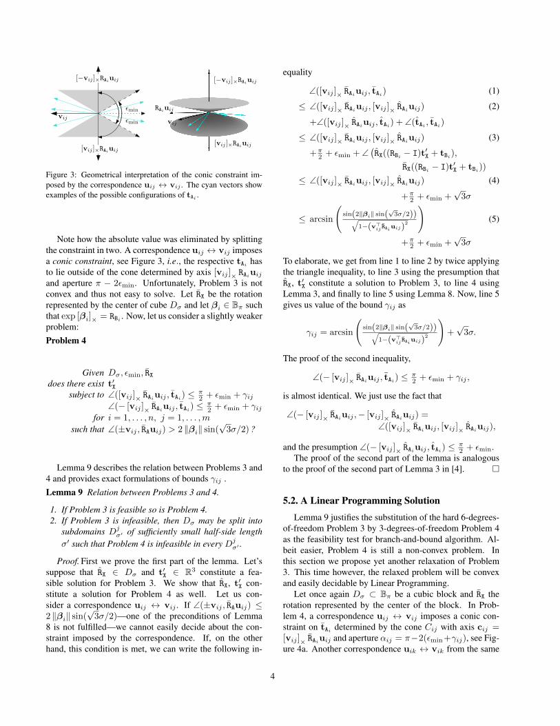
Figure 3: Geometrical interpretation of the conic constraint im-posed by the correspondence uij ↔ vij . The cyan vectors showexamples of the possible configurations of tAi .

Note how the absolute value was eliminated by splittingthe constraint in two. A correspondence uij ↔ vij imposesa conic constraint, see Figure 3, i.e., the respective tAi hasto lie outside of the cone determined by axis [vij ]× RAiuijand aperture π − 2εmin. Unfortunately, Problem 3 is notconvex and thus not easy to solve. Let RX be the rotationrepresented by the center of cube Dσ and let βi ∈ Bπ suchthat exp [βi]× = RBi . Now, let us consider a slightly weakerproblem:Problem 4

Given Dσ, εmin, RXdoes there exist t′X

subject to ∠([vij ]× RAiuij , tAi) ≤ π2 + εmin + γij

∠(− [vij ]× RAiuij , tAi) ≤ π2 + εmin + γij

for i = 1, . . . , n, j = 1, . . . ,m

such that ∠(±vij , RAuij) > 2 ‖βi‖ sin(√

3σ/2) ?

Lemma 9 describes the relation between Problems 3 and4 and provides exact formulations of bounds γij .Lemma 9 Relation between Problems 3 and 4.

1. If Problem 3 is feasible so is Problem 4.2. If Problem 3 is infeasible, then Dσ may be split into

subdomains Djσ′ of sufficiently small half-side length

σ′ such that Problem 4 is infeasible in every Djσ′ .

Proof. First we prove the first part of the lemma. Let’ssuppose that RX ∈ Dσ and t′X ∈ R3 constitute a fea-sible solution for Problem 3. We show that RX, t′X con-stitute a solution for Problem 4 as well. Let us con-sider a correspondence uij ↔ vij . If ∠(±vij , RAuij) ≤2 ‖βi‖ sin(

√3σ/2)—one of the preconditions of Lemma

8 is not fulfilled—we cannot easily decide about the con-straint imposed by the correspondence. If, on the otherhand, this condition is met, we can write the following in-

equality

∠([vij ]× RAiuij , tAi) (1)

≤ ∠([vij ]× RAiuij , [vij ]× RAiuij) (2)

+∠([vij ]× RAiuij , tAi) + ∠(tAi , tAi)

≤ ∠([vij ]× RAiuij , [vij ]× RAiuij) (3)

+π2 + εmin + ∠

(RX((RBi − I)t′X + tBi),

RX((RBi − I)t′X + tBi))

≤ ∠([vij ]× RAiuij , [vij ]× RAiuij) (4)

+π2 + εmin +

√3σ

≤ arcsin

(sin(2‖βi‖ sin(

√3σ/2))√

1−(v>ij RAiuij)2

)(5)

+π2 + εmin +

√3σ

To elaborate, we get from line 1 to line 2 by twice applyingthe triangle inequality, to line 3 using the presumption thatRX, t′X constitute a solution to Problem 3, to line 4 usingLemma 3, and finally to line 5 using Lemma 8. Now, line 5gives us value of the bound γij as

γij = arcsin

(sin(2‖βi‖ sin(

√3σ/2))√

1−(v>ij RAiuij)2

)+√

3σ.

The proof of the second inequality,

∠(− [vij ]× RAiuij , tAi) ≤ π2 + εmin + γij ,

is almost identical. We just use the fact that

∠(− [vij ]× RAiuij ,− [vij ]× RAiuij) =

∠([vij ]× RAiuij , [vij ]× RAiuij),

and the presumption ∠(− [vij ]× RAiuij , tAi) ≤ π2 + εmin.

The proof of the second part of the lemma is analogousto the proof of the second part of Lemma 3 in [4]. �

5.2. A Linear Programming Solution

Lemma 9 justifies the substitution of the hard 6-degrees-of-freedom Problem 3 by 3-degrees-of-freedom Problem 4as the feasibility test for branch-and-bound algorithm. Al-beit easier, Problem 4 is still a non-convex problem. Inthis section we propose yet another relaxation of Problem3. This time however, the relaxed problem will be convexand easily decidable by Linear Programming.

Let once again Dσ ⊂ Bπ be a cubic block and RX therotation represented by the center of the block. In Prob-lem 4, a correspondence uij ↔ vij imposes a conic con-straint on tAi determined by the cone Cij with axis cij =[vij ]× RAiuij and aperture αij = π−2(εmin+γij), see Fig-ure 4a. Another correspondence uik ↔ vik from the same

4

RAiuij

vij

−cij

Cij

(a)

RAiuik

vik

−cik

Cij

Cik

l1ijk

l2ijk

l3ijk

l4ijk

(b)

n1ijk

n4ijk

n2ijk

n3ijk

(c)

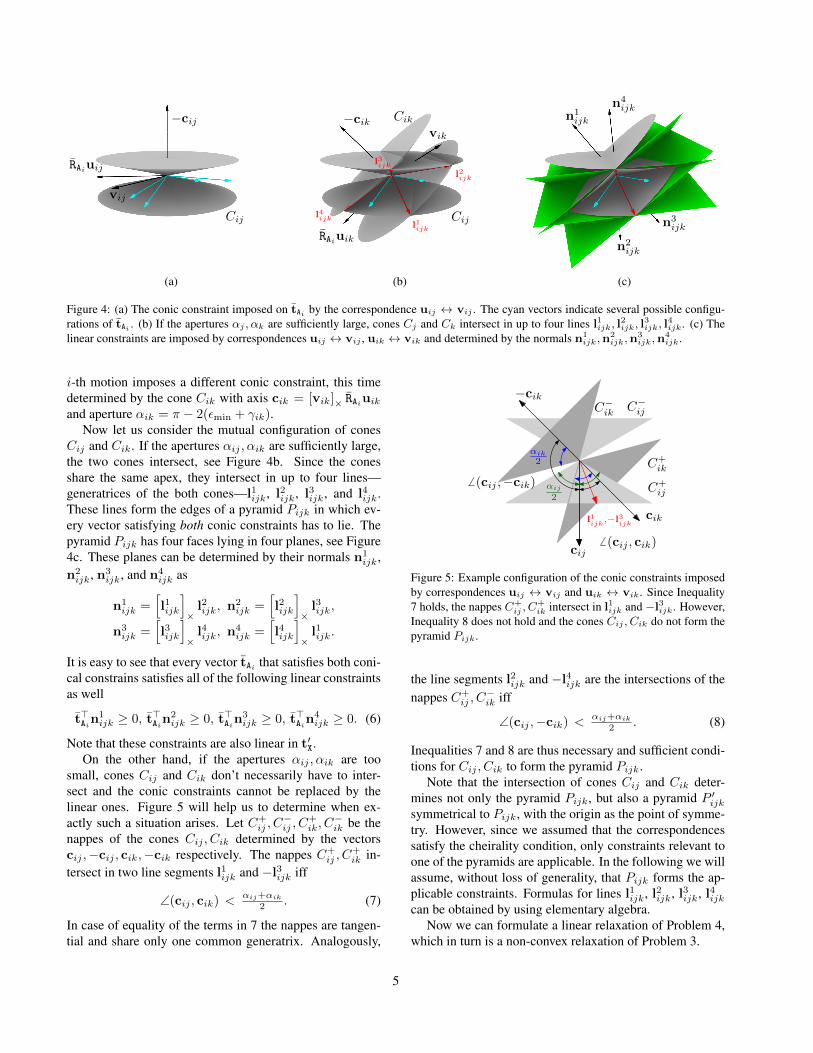
Figure 4: (a) The conic constraint imposed on tAi by the correspondence uij ↔ vij . The cyan vectors indicate several possible configu-rations of tAi . (b) If the apertures αj , αk are sufficiently large, cones Cj and Ck intersect in up to four lines l1ijk, l

2ijk, l

3ijk, l

4ijk. (c) The

linear constraints are imposed by correspondences uij ↔ vij , uik ↔ vik and determined by the normals n1ijk,n

2ijk,n

3ijk,n

4ijk.

i-th motion imposes a different conic constraint, this timedetermined by the cone Cik with axis cik = [vik]× RAiuikand aperture αik = π − 2(εmin + γik).

Now let us consider the mutual configuration of conesCij and Cik. If the apertures αij , αik are sufficiently large,the two cones intersect, see Figure 4b. Since the conesshare the same apex, they intersect in up to four lines—generatrices of the both cones—l1ijk, l2ijk, l3ijk, and l4ijk.These lines form the edges of a pyramid Pijk in which ev-ery vector satisfying both conic constraints has to lie. Thepyramid Pijk has four faces lying in four planes, see Figure4c. These planes can be determined by their normals n1

ijk,n2ijk, n3

ijk, and n4ijk as

n1ijk =

[l1ijk

]×l2ijk, n

2ijk =

[l2ijk

]×l3ijk,

n3ijk =

[l3ijk

]×l4ijk, n

4ijk =

[l4ijk

]×l1ijk.

It is easy to see that every vector tAi that satisfies both coni-cal constrains satisfies all of the following linear constraintsas well

t>Ain1ijk ≥ 0, t>Ain

2ijk ≥ 0, t>Ain

3ijk ≥ 0, t>Ain

4ijk ≥ 0. (6)

Note that these constraints are also linear in t′X.On the other hand, if the apertures αij , αik are too

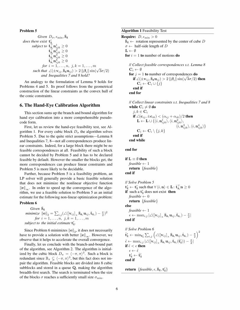
small, cones Cij and Cik don’t necessarily have to inter-sect and the conic constraints cannot be replaced by thelinear ones. Figure 5 will help us to determine when ex-actly such a situation arises. Let C+

ij , C−ij , C

+ik, C

−ik be the

nappes of the cones Cij , Cik determined by the vectorscij ,−cij , cik,−cik respectively. The nappes C+

ij , C+ik in-

tersect in two line segments l1ijk and −l3ijk iff

∠(cij , cik) <αij+αik

2 . (7)

In case of equality of the terms in 7 the nappes are tangen-tial and share only one common generatrix. Analogously,

cik

−cik

C+ik

αij

2

αik

2

6 (cij ,−cik)

6 (cij , cik)

C−ijC−

ik

C+ij

cij

l1ijk

,−l3ijk

Figure 5: Example configuration of the conic constraints imposedby correspondences uij ↔ vij and uik ↔ vik. Since Inequality7 holds, the nappes C+

ij , C+ik intersect in l1ijk and−l3ijk. However,

Inequality 8 does not hold and the cones Cij , Cik do not form thepyramid Pijk.

the line segments l2ijk and −l4ijk are the intersections of thenappes C+

ij , C−ik iff

∠(cij ,−cik) <αij+αik

2 . (8)

Inequalities 7 and 8 are thus necessary and sufficient condi-tions for Cij , Cik to form the pyramid Pijk.

Note that the intersection of cones Cij and Cik deter-mines not only the pyramid Pijk, but also a pyramid P ′ijksymmetrical to Pijk, with the origin as the point of symme-try. However, since we assumed that the correspondencessatisfy the cheirality condition, only constraints relevant toone of the pyramids are applicable. In the following we willassume, without loss of generality, that Pijk forms the ap-plicable constraints. Formulas for lines l1ijk, l2ijk, l3ijk, l4ijkcan be obtained by using elementary algebra.

Now we can formulate a linear relaxation of Problem 4,which in turn is a non-convex relaxation of Problem 3.

5

Problem 5Given Dσ, εmin, RX

does there exist t′Xsubject to t>Ain

1ijk ≥ 0

t>Ain2ijk ≥ 0

t>Ain3ijk ≥ 0

t>Ain4ijk ≥ 0

for i = 1, . . . , n, j, k = 1, . . . ,m

such that ∠(±vij , RAuij) > 2 ‖βi‖ sin(√

3σ/2)and Inequalities 7 and 8 hold?

An analogy to the formulation of Lemma 9 holds forProblems 4 and 5. Its proof follows from the geometricalconstruction of the linear constraints as the convex hull ofthe conic constraints.

6. The Hand-Eye Calibration AlgorithmThis section sums up the branch and bound algorithm for

hand eye calibration into a more comprehensible pseudo-code form.

First, let us review the hand-eye feasibility test, see Al-gorithm 1. For every cubic block Dσ the algorithm solvesProblem 5. Due to the quite strict assumptions—Lemma 8and Inequalities 7, 8—not all correspondences produce lin-ear constraints. Indeed, for a large block there might be nofeasible correspondences at all. Feasibility of such a blockcannot be decided by Problem 5 and it has to be declaredfeasible by default. However the smaller the blocks get, themore correspondences can produce linear constraints andProblem 5 is more likely to be decidable.

Further, because Problem 5 is a feasibility problem, anLP solver will generally provide a basic feasible solutionthat does not minimize the nonlinear objective function‖e‖∞. In order to speed up the convergence of the algo-rithm, we use a feasible solution to Problem 5 as an initialestimate for the following non-linear optimization problem:Problem 6

Given RXminimize ‖e‖2 =

∑i,j(∠([vij ]× RAiuij , tAi)− π

2 )2

for i = 1, . . . , n, j, k = 1, . . . ,msubject to the initial estimate t′X.

Since Problem 6 minimizes ‖e‖2, it does not necessarilyhave to provide a solution with better ‖e‖∞. However, weobserve that it helps to accelerate the overall convergence.

Finally, let us conclude with the branch-and-bound partof the algorithm, see Algorithm 2. The algorithm is initial-ized by the cubic block Dπ = 〈−π, π〉3. Such a block isredundant since Bπ ( 〈−π, π〉3, but this fact does not im-pair the algorithm. Feasible blocks are divided into 8 cubicsubblocks and stored in a queue Q, making the algorithmbreadth-first search. The search is terminated when the sizeof the blocks σ reaches a sufficiently small size σmin.

Algorithm 1 Feasibility Test

Require: D, εmin > 0RX ← rotation represented by the center of cube Dσ ← half-side length of DL← ∅for i = 1 to number of motions do

// Collect feasible correspondences s.t. Lemma 8Ci ← ∅for j = 1 to number of correspondences do

if ∠(±vij , RAuij) > 2 ‖βi‖ sin(√

3σ/2) thenCi ← Ci ∪ {j}

end ifend for

// Collect linear constraints s.t. Inequalities 7 and 8while Ci 6= ∅ doj, k ∈ Ci

if ∠(cij ,±cik) < (αij + αik)/2 thenL← L ∪ {〈i,n1

ijk〉, 〈i,n2ijk〉,〈i,n3

ijk〉, 〈i,n4ijk〉}

Ci ← Ci \ {j, k}end if

end while

end for

if L ≡ ∅ thenfeasible← 1return {feasible}

end if

// Solve Problem 5t′X ← t′X such that ∀ 〈i,n〉 ∈ L : t>Ain ≥ 0if such a t′X does not exist then

feasible← 0return {feasible}

elsefeasible← 1ε← maxi,j |∠([vij ]× RAiuij , tAi)− π

2 |end if

// Solve Problem 6t′X ← mint′X

∑i,j

(∠([vij ]× RAiuij , tAi)− π

2

)2

ε← maxi,j |∠([vij ]× RAiuij , tAi(t′X))− π

2 |if ε < ε thenε← εt′X ← t′X

end if

return {feasible, ε, RX, t′X}

6

Algorithm 2 Branch and Bound

Require: initial estimate of εmin, stopping criterion σmin

Dπ ← 〈−π, π〉3PushBack(Q, Dπ)σ ← 2πwhile σ > σmin doD ← PopFront(Q)σ ← half-side length of D{feasible, ε, RX, t′X} ← FeasibilityTest(D, εmin)if feasible ≡ true then

if ε < εmin thenRX ← RXt′X ← t′Xεmin ← ε

end ifPushBack(Q,SubdivideBlock(D)

end ifend whiletX ← −RXt′Xreturn {RX, tX, εmin}

7. Experimental ResultsNext, the performance of the proposed algorithm is eval-

uated using both synthetically generated and real world datameasurements. We use GLPK [1] to solve Problem 5 andlevmar [8] to solve nonlinear Problem 6. The values of theinitial estimate εmin and the stopping criterion σmin wereset to 0.02 and 0.0005 respectively. All the reported timeswere achieved on a 3GHz Intel Core i7 based desktop com-puter running 64-bit Linux. The source code is available athttp://cmp.felk.cvut.cz/∼hellej1/bbhec/.

7.1. Experiment with Synthetic Data

A synthetic scene consisting of 100 3D points was gen-erated into a ball of radius 1,000 mm. 10 absolute ca-mera poses were set up so that (i) the centers of the cam-eras were outside the ball but close to its ‘surface’, (ii) thecenters were positioned so that the offsets of the cameramotions would be ˜500 mm and (iii) the cameras faced ap-proximately the center of the ball. In order to simulate theeffect of decreasing field of view (FOV), 7 progressivelysmaller balls were generated inside the initial ball so that theballs shared the centers and the volume of the newly createdball was half the volume of the previous ball. This defined8 FOV levels, namely 180◦, 105◦, 78◦, 60◦, 47◦, 37◦, 29◦,and 23◦. Additional 3D points were generated inside eachof the smaller balls in order to have exactly 100 3D pointsat each FOV level measured in the respective cameras giv-ing raise to correspondences uij ↔ vij (newly generatedpoints did not contribute to the larger balls).

σ2 of the Gaussian noise||

e||∞

ofth

eob

tain

edso

lutio

n[r

ad]

00 10.2 0.4 0.6 0.8

0.002

0.004

0.006

0.008

0.01

0.012

0.014

×10-3

(a)

Euc

lidea

ner

ror

of3D

poin

ts[m

m]

σ2 of the Gaussian noise

narrowstandardwide

00

1

1

2

3

4

5

6

7

0.2 0.4 0.6 0.8

×10-3

(b)

Number of subdivisions

Num

ber

ofcu

bes

narrowstandardwide

10

10

10

1010 12

2

3

4

5

4 6 8

(c)Number of subdivisions||

e||∞

ofth

eob

tain

edso

lutio

n[r

ad]

lowmediumhigh

10 1204 6 8

0.01

0.005

0.015

0.02

(d)

Figure 6: Synthetic data experiment. (a) The maximum residualerror of the obtained solutions for the various values of σ2(redline) and the distribution of the measured errors over all corre-spondences (boxes). (b) The mean Euclidean distance between the3D points transformed to the gripper’s coordinate systems usingground truth X and the 3D points transformed to the gripper’s co-ordinate systems using the estimated X. Different FOV levels wereclustered into three groups. (c) The mean number of remainingcubes plotted against the number of subdivision phases. Note thatthe computation starts after the fourth subdivision. (d) The meanresidual error at the beginning of the respective subdivision phase.Different noise levels were clustered into three groups.

Further, ten random transformations X were generatedand the optimization tasks composed of the known corre-spondences uij ↔ vij and 9 motions Bi—computed fromthe known absolute camera poses and the generated X—were constructed for each of the 8 FOV levels. Finally, thecorrespondences were corrupted with Gaussian noise in theangular domain using 11 noise levels, σ2 ∈

⟨0, 10−3⟩ in

10−4 steps resulting to 88 tasks per transformation.The results of the experiment are shown in Figure 6.

Note that the median of the measured errors over all cor-respondences is approximately one order of magnitudesmaller than the maximum residual error. The actual errorsof the calibration—being the Euclidean distance betweenthe 3D points transformed to the gripper’s coordinate sys-tems using ground truth X and the 3D points transformed tothe gripper’s coordinate systems using the estimated X—arelower for wide FOV. Considering the timings resulting fromboth single-threaded and multi-threaded C++ implementa-tions of the algorithm,

narrow FOV standard FOV wide FOV1 thread 1985.5 s 792.7 s 478.7 s8 threads 430.4 s 168.0 s 101.5 s

7

(a) (b)

Figure 7: Real data experiment. (a) Close up of the camera-gripperrig, sample images from the sequence. (b) Model resulting fromSfM, cameras are denoted by red pyramids.

the solutions are found faster for wide FOV as the corre-spondences of narrow FOV camera pairs do not generateenough linear constraints for large blocks and thus moreblocks are subdivided.

7.2. Experiment with Real Data

A Mitsubishi MELFA-RV-6S serial manipulator with aCanon 7D digital SLR camera and a Sigma 8 mm lens (pixelsize ˜0.0011 rad, FOV ˜130◦) were used to acquire the datafor the real experiment. The robot was instructed to movethe gripper along the surface of a sphere of radius ˜700 mmcentered in the middle of the scene objects. The positionof the gripper was adjusted using the yaw and pitch anglesmeasured from the center of the sphere to reach 25 differentlocations at four different pitch angles and the gripper wasset to face the center of the sphere, see Figure 7a.

The internal calibration of the camera was obtained fromseveral images of a checkerboard using OCamCalib [9] asa polynomial model of degree 3. A state-of-the-art sequen-tial SfM software [12] was used to automatically generateimage feature points, match them, verify the matches bypairwise epipolar geometries, and create tracks and triangu-lated 3D points, see Figure 7b. We used 24 motions Bi and100 correspondences uij ↔ vij per motion—randomly se-lected from the feature tracks—to construct the optimiza-tion task. Note that the knowledge of the relative cameraposes Ai and the triangulated 3D points was not used.

We executed the task for εmin being 0.1 and received asolution with residual error ‖e‖∞ = 0.0414 rad (median ofthe measured errors 0.0055 rad) in 1572.8 seconds (runningin 8 threads). The computed rotation RX was close to therotation along the z-axis by π/4 as expected.

8. ConclusionIn this paper we removed the requirement for known ca-

mera extrinsics from hand-eye calibration problem. Since

the presented algorithm is completely independent on thescene geometry and scale, there is no need for a known ca-libration device and the calibration can be performed solelyfrom a general scene. The algorithm solves for both the un-known rotation and translation simultaneously and is guar-anteed to be globally optimal with respect to L∞-norm.

Acknowledgment The authors were supported by the ECunder projects FP7-SPACE-218814 PRoVisG and FP7-SPACE-241523 PRoViScout and by Grant Agency of the CTU Pragueproject SGS10/277/OHK3/3T/13. The authors would also like tothank Martin Meloun for his help with the real-data experiment.

References[1] GNU linear programming kit version 4.47, 2011,

http://www.gnu.org/software/glpk/glpk.html

[2] J. C. K. Chou and M. Kamel. Finding the position and orien-tation of a sensor on a robot manipulator using quaternions.IJRR, 10(3):240–254, 1991.

[3] K. Daniilidis. Hand-eye calibration using dual quaternions.IJRR, 18:286–298, 1998.

[4] R. Hartley and F. Kahl. Global optimization through rotationspace search. IJCV, 82(1):64–79, 2009.

[5] R. Hartley and A. Zisserman. Multiple View Geometry inComputer Vision. Cambridge University Press, 2003.

[6] J. Heller, M. Havlena, A. Sugimoto, and T. Pajdla. Structure-from-motion based hand-eye calibration using L∞ mini-mization. In CVPR, pp. 3497–3503, 2011.

[7] R. Horaud and F. Dornaika. Hand-eye calibration. IJRR,14(3):195–210, 1995.

[8] M. Lourakis. levmar: Levenberg-marquardt non-linear least squares algorithms in C/C++, 2004,http://www.ics.forth.gr/∼lourakis/levmar/

[9] D. Scaramuzza, A. Martinelli, and R. Siegwart. A toolboxfor easily calibrating omnidirectional cameras. In Interna-tional Conference on Intelligent Robots and Systems, pp.5695–5701, 2006.

[10] Y. Seo, Y.-J. Choi, and S. W. Lee. A branch-and-boundalgorithm for globally optimal calibration of a camera-and-rotation-sensor system. In ICCV, pp. 1173–1178, 2009.

[11] Y. Shiu and S. Ahmad. Calibration of wrist-mounted roboticsensors by solving homogeneous transform equations of theform AX=XB. IEEE Transactions on Robotics and Automa-tion, 5(1):16–29, 1989.

[12] A. Torii, M. Havlena, and T. Pajdla. Omnidirectional imagestabilization for visual object recognition. IJCV, 91(2):157–174, 2011.

[13] R. Tsai and R. Lenz. Real time versatile robotics hand/eyecalibration using 3d machine vision. In International Confer-ence on Robotics and Automation, pp. 554–561 vol.1, 1988.

[14] R. Tsai and R. Lenz. A new technique for fully autonomousand efficient 3d robotics hand/eye calibration. IEEE Trans-actions on Robotics and Automation, 5(3):345–358, 1989.

[15] H. Zhang. Hand/eye calibration for electronic assemblyrobots. IEEE Transactions on Robotics and Automation,14(4):612–616, 1998.

8