HAL Id: hal-02905816https://hal.archives-ouvertes.fr/hal-02905816v2

Preprint submitted on 2 Sep 2021

HAL is a multi-disciplinary open accessarchive for the deposit and dissemination of sci-entific research documents, whether they are pub-lished or not. The documents may come fromteaching and research institutions in France orabroad, or from public or private research centers.

L’archive ouverte pluridisciplinaire HAL, estdestinée au dépôt et à la diffusion de documentsscientifiques de niveau recherche, publiés ou non,émanant des établissements d’enseignement et derecherche français ou étrangers, des laboratoirespublics ou privés.

Globally Optimal Solution to Inverse Kinematics of7DOF Serial Manipulator

Pavel Trutman, Mohab Safey El Din, Didier Henrion, Tomas Pajdla

To cite this version:Pavel Trutman, Mohab Safey El Din, Didier Henrion, Tomas Pajdla. Globally Optimal Solution toInverse Kinematics of 7DOF Serial Manipulator. 2021. �hal-02905816v2�

Globally Optimal Solution to Inverse Kinematics of 7DOF SerialManipulator

Pavel TrutmanFEE and CIIRC CTU in Prague

Mohab Safey El DinSorbonne Université, LIP6 CNRS

Didier HenrionLAAS-CNRS, FEE CTU in Prague

Tomas PajdlaCIIRC CTU in Prague

September 2, 2021

AbstractThe Inverse Kinematics (IK) problem is concerned with finding robot control parameters to

bring the robot into a desired position under the kinematics and collision constraints. We presenta global solution to the optimal IK problem for a general serial 7DOF manipulator with revolutejoints and a quadratic polynomial objective function. We show that the kinematic constraints dueto rotations can be all generated by the second-degree polynomials. This is an important result sinceit significantly simplifies the further step where we find the optimal solution by Lasserre relaxationsof nonconvex polynomial systems. We demonstrate that the second relaxation is sufficient to solvea general 7DOF IK problem. Our approach is certifiably globally optimal. We demonstrate themethod on the 7DOF KUKA LBR IIWA manipulator and show that we are in practice able tocompute the optimal IK or certify infeasibility in 99.9 % tested poses. We also demonstrate thatby the same approach, we are able to solve the IK problem for a random generic manipulator withseven revolute joints.

1 Introduction

The Inverse Kinematics (IK) problem is one of the most important problems in robotics [33]. Thesolution to the IK problem finds robot control parameters to bring the robot into a desired positionunder the kinematics and collision constraints [14].

The IK problem has been extensively studied in robotics and control [30, 31]. The classical formu-lation [30] of the problem for 6 degrees of freedom (6DOF) serial manipulators leads to solving a systemof polynomial equations [6, 34]. This is, in general, a hard (“EXPSPACE complete” [26]) algebraiccomputational problem, but practical solving methods have been developed for 6DOF manipulators[30, 24, 9].

An important generalization of the IK problem aims at finding the optimal control parametersfor an underconstrained mechanism, i.e., when the number of controlled joints in a manipulator islarger than six. Then, an algebraic computation problem turns into an optimization problem overan algebraic variety [6] of possible IK solutions. It is particularly convenient to choose a polynomialobjective function to arrive at a semialgebraic optimization problem.

Semi-algebraic optimization problems are in general nonconvex, but they can be solved with certi-fied global optimality [21] using the Lasserre hierarchy of convex optimization problems [20]. Compu-tationally, however, semialgebraic optimization problems are in general extremely hard and were oftenconsidered too expensive to be used in practice. In this paper, we show that using “algebraic prepro-cessing”, semialgebraic optimization methods become practical in solving the IK problem of general7DOF serial manipulators with a polynomial objective function.

1.1 Contribution

Our main contributions are as follows.

1

-800-600-400-200 0 200 400 600 800-800-600-400-2000200400600800

01002003004005006007008009001000

x [mm]

y [mm]

z [mm]

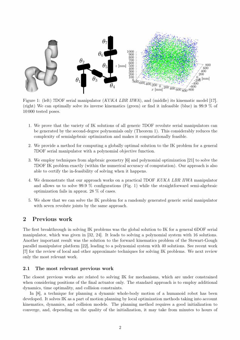
Figure 1: (left) 7DOF serial manipulator (KUKA LBR IIWA), and (middle) its kinematic model [17].(right) We can optimally solve its inverse kinematics (green) or find it infeasible (blue) in 99.9 % of10 000 tested poses.

1. We prove that the variety of IK solutions of all generic 7DOF revolute serial manipulators canbe generated by the second-degree polynomials only (Theorem 1). This considerably reduces thecomplexity of semialgebraic optimization and makes it computationally feasible.

2. We provide a method for computing a globally optimal solution to the IK problem for a general7DOF serial manipulator with a polynomial objective function.

3. We employ techniques from algebraic geometry [6] and polynomial optimization [21] to solve the7DOF IK problem exactly (within the numerical accuracy of computation). Our approach is alsoable to certify the in-feasibility of solving when it happens.

4. We demonstrate that our approach works on a practical 7DOF KUKA LBR IIWA manipulatorand allows us to solve 99.9 % configurations (Fig. 1) while the straightforward semi-algebraicoptimization fails in approx. 28 % of cases.

5. We show that we can solve the IK problem for a randomly generated generic serial manipulatorwith seven revolute joints by the same approach.

2 Previous work

The first breakthrough in solving IK problems was the global solution to IK for a general 6DOF serialmanipulator, which was given in [32, 24]. It leads to solving a polynomial system with 16 solutions.Another important result was the solution to the forward kinematics problem of the Stewart-Goughparallel manipulator platform [22], leading to a polynomial system with 40 solutions. See recent work[7] for the review of local and other approximate techniques for solving IK problems. We next reviewonly the most relevant work.

2.1 The most relevant previous work

The closest previous works are related to solving IK for mechanisms, which are under constrainedwhen considering positions of the final actuator only. The standard approach is to employ additionaldynamics, time optimality, and collision constraints.

In [8], a technique for planning a dynamic whole-body motion of a humanoid robot has beendeveloped. It solves IK as a part of motion planning by local optimization methods taking into accountkinematics, dynamics, and collision models. The planning method requires a good initialization toconverge, and, depending on the quality of the initialization, it may take from minutes to hours of

2

running time. Our approach provides a globally optimal solution for 7DOF kinematics subchains ofmore complex mechanisms and could be used to initialize the kinematic part of motion planning.

Work [17] presented an IK solution for 7DOF manipulators with zero link offsets, e.g., the KUKALBR IIWA manipulators. The solution uses special kinematics of its class of manipulators to decomposethe general IK problem into two simpler IK problems that can be solved in a closed form. The one-dimensional variety of self-motions becomes circular, and hence the paper proposes to parameterize it bythe angle of a point of the circle. Our approach generalizes this solution to a general 7DOF manipulatorand shows that it is feasible to solve the IK problem for completely general 7DOF manipulators andoptimize over their self-motion varieties.

Paper [7] presents a global (but only approximate) solution to the IK for 7DOF manipulators. Itformulates the IK problem as a mixed-integer convex optimization program. The key idea of the paperis to approximate the nonconvex space of rotations by piecewise linear functions on several intervalsthat partition the original space. This turns the original nonconvex problem into an approximateconvex problem when a correct interval is chosen. Selecting the values of auxiliary binary variablesto pick the actual interval of approximation leads to the integer part of the optimization. This wasthe first practical globally optimal approach, but it is only approximate and delivers solutions witherrors in units of centimeters and units of degrees. It also fails to detect about 5 % of infeasible poses.Our approach solves the original problem with sub-10−6 mm and sub-10−3 degree error, and we cansolve/decide the feasibility in all but 0.1 % of the tested cases. The computation times of [7] and ourapproach are roughly similar in units of seconds.

A global and precise solution to the IK problem for redundant serial manipulators is presented in[25]. It models the kinematic constraints as a distance geometry problem. Alongside a novel formulationof the joint limit constraints, it delivers quadratic constraints only. The final configuration is found asthe nearest configuration to the given one while satisfying the quadratic constraints. This approachleads to a QCQP problem, which is solved by an SDP relaxation with a global optimality certificateand infeasibility detection. Their implementation is fast (2.5 ms per pose) and accurate (sub-10−2 mmposition error) with the failure rate of less than 0.4 %. This formulation is restricted only to revolutejoints for planar manipulators and spherical joints for three-dimensional ones. It does not take intoaccount the full rotation of each link and can thus solve only for simplified situations. In contrast,our method is general and applicable to any serial manipulator with revolute joints. Moreover, anyspherical joint can be modeled as three revolute joints with the advantage of finer control of the jointangle limits.

3 Problem formulation

Here we formulate the IK problem for 7DOF serial manipulators as a semialgebraic optimizationproblem with a polynomial objective function.

The task is to find the joint coordinates of the manipulator in a way that the end-effector reachesthe desired pose in space. The IK problem is called underconstrained for manipulators, which havemore DOF than they require to execute the given task. In our case, to reach the desired pose in space,the manipulators require to have six DOFs, and therefore the IK problem for a 7DOF manipulatoris underconstrained. The consequence is that the IK problem has an infinite number of solutions forreachable generic end-effector poses for such manipulators. This results in the self-motion propertyof these manipulators. A self-motion is a motion of a manipulator, which is not observed in the taskspace, i.e., the end-effector pose of the manipulator is constant while the links of the manipulator aremoving. Therefore, moving the manipulator along a path consisting of joint configurations of differentsolutions of the IK problem for the same pose in space, will result in a self-motion of the manipulator.

The self-motion property provides the manipulator more adaptability since it allows, e.g., to avoidmore obstacles in the path and to avoid singularities, which leads to a more versatile mechanism. Onthe other hand, increasing the number of degrees of freedom increases the difficulty of the IK problemcomputation dramatically. The IK problem has no longer a finite number of solutions, and thus, it ismeaningful to formulate it as a constrained optimization problem choosing the optimal solution fromthe set of all feasible solutions.

3

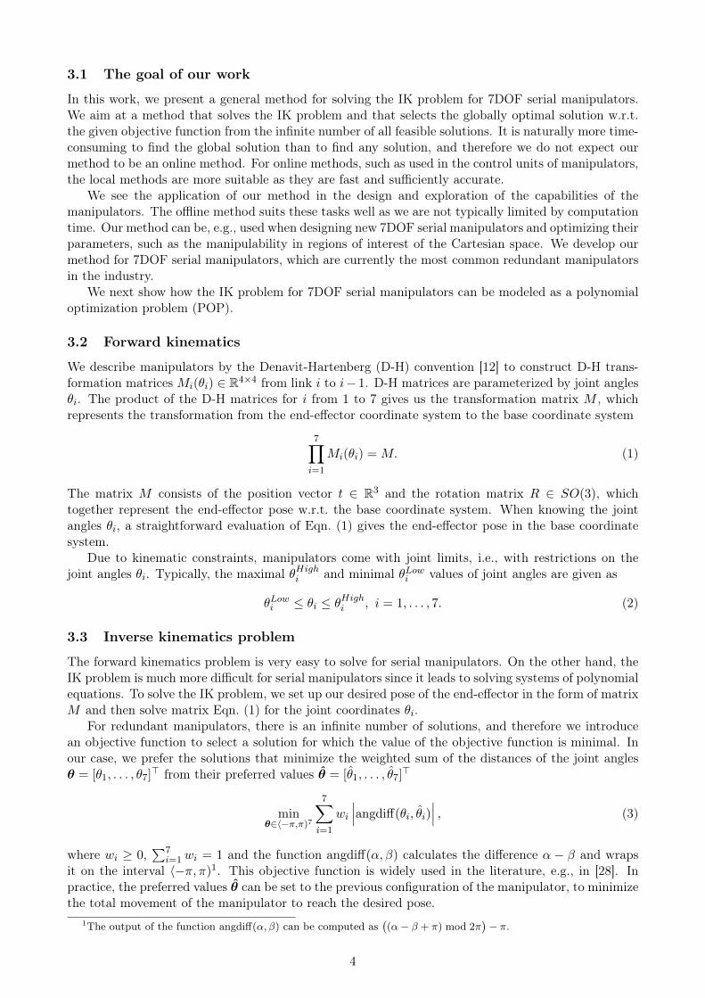
3.1 The goal of our work

In this work, we present a general method for solving the IK problem for 7DOF serial manipulators.We aim at a method that solves the IK problem and that selects the globally optimal solution w.r.t.the given objective function from the infinite number of all feasible solutions. It is naturally more time-consuming to find the global solution than to find any solution, and therefore we do not expect ourmethod to be an online method. For online methods, such as used in the control units of manipulators,the local methods are more suitable as they are fast and sufficiently accurate.

We see the application of our method in the design and exploration of the capabilities of themanipulators. The offline method suits these tasks well as we are not typically limited by computationtime. Our method can be, e.g., used when designing new 7DOF serial manipulators and optimizing theirparameters, such as the manipulability in regions of interest of the Cartesian space. We develop ourmethod for 7DOF serial manipulators, which are currently the most common redundant manipulatorsin the industry.

We next show how the IK problem for 7DOF serial manipulators can be modeled as a polynomialoptimization problem (POP).

3.2 Forward kinematics

We describe manipulators by the Denavit-Hartenberg (D-H) convention [12] to construct D-H trans-formation matrices Mi(θi) ∈ R4×4 from link i to i− 1. D-H matrices are parameterized by joint anglesθi. The product of the D-H matrices for i from 1 to 7 gives us the transformation matrix M , whichrepresents the transformation from the end-effector coordinate system to the base coordinate system

7∏i=1

Mi(θi) = M. (1)

The matrix M consists of the position vector t ∈ R3 and the rotation matrix R ∈ SO(3), whichtogether represent the end-effector pose w.r.t. the base coordinate system. When knowing the jointangles θi, a straightforward evaluation of Eqn. (1) gives the end-effector pose in the base coordinatesystem.

Due to kinematic constraints, manipulators come with joint limits, i.e., with restrictions on thejoint angles θi. Typically, the maximal θHighi and minimal θLowi values of joint angles are given as

θLowi ≤ θi ≤ θHighi , i = 1, . . . , 7. (2)

3.3 Inverse kinematics problem

The forward kinematics problem is very easy to solve for serial manipulators. On the other hand, theIK problem is much more difficult for serial manipulators since it leads to solving systems of polynomialequations. To solve the IK problem, we set up our desired pose of the end-effector in the form of matrixM and then solve matrix Eqn. (1) for the joint coordinates θi.

For redundant manipulators, there is an infinite number of solutions, and therefore we introducean objective function to select a solution for which the value of the objective function is minimal. Inour case, we prefer the solutions that minimize the weighted sum of the distances of the joint anglesθ = [θ1, . . . , θ7]

> from their preferred values θ = [θ1, . . . , θ7]>

minθ∈〈−π,π)7

7∑i=1

wi

∣∣∣angdiff(θi, θi)∣∣∣ , (3)

where wi ≥ 0,∑7

i=1wi = 1 and the function angdiff(α, β) calculates the difference α − β and wrapsit on the interval 〈−π, π)1. This objective function is widely used in the literature, e.g., in [28]. Inpractice, the preferred values θ can be set to the previous configuration of the manipulator, to minimizethe total movement of the manipulator to reach the desired pose.

1The output of the function angdiff(α, β) can be computed as((α− β + π) mod 2π

)− π.

4

Next, we add the joint limits to obtain the following optimization problem

minθ∈〈−π,π)7

7∑i=1

wi

∣∣∣angdiff(θi, θi)∣∣∣

s.t.∏7i=1Mi(θi) = M

θLowi ≤ θi ≤ θHighi (i = 1, . . . , 7)

(4)

To be able to use the techniques of polynomial optimization, we need to remove the trigonometricfunctions that appear in Eqn. (1). We do that by introducing new variables c = [c1, . . . , c7]

> ands = [s1, . . . , s7]

>, which represent the cosines and sines of the joint angles θ = [θ1, . . . , θ7]>, respectively.

Then, we can rewrite Problem (4) in the new variables. To preserve the structure of the problem, weneed to add the trigonometric identities

qi(c, s) = c2i + s2i − 1 = 0, i = 1, . . . , 7. (5)

Matrix Eqn. (1) contains 12 trigonometric equations and can be directly rewritten as 12 polynomialequations of degrees up to seven in the newly introduced variables. To lower the maximal degree of theequations, we use fact that the inverse of a rotation matrix is its transpose, i.e., it is a linear functionof the original rotation matrix, and rewrite Eqn. (1) as

5∏i=3

Mi(θi)−M−12 (θ2)M−11 (θ1)MM−17 (θ7)M

−16 (θ6) = 0. (6)

It reduces the maximal degree of the polynomials in unknowns c and s to four. We denote thesepolynomials in Eqn. (6) as

pj(c, s) = 0, j = 1, . . . , 12. (7)

The next step is to change the objective function (3) to a polynomial in the new variables c, s.Instead of evaluating the distance between the joint angles and their preferred values, we can do thesame in the space of their cosines and sines to reach the same goal, i.e., to get θ as close as possible toθ. Choosing the proper `p norm for the problem at hand may lead to a more straightforward solutionto the problem (e.g., the `∞ norm is often used in multiple view geometry problems [15] to obtain aconvex relaxation of the original problem). We have decided to use the squared `2 norm on the cosinesand sines since it leads to an objective function, which is linear in the new variables c and s:

minc∈〈−1,1〉7, s∈〈−1,1〉7

7∑i=1

wi

((ci − cos θi)

2 + (si − sin θi)2)

(8)

= minc∈〈−1,1〉7, s∈〈−1,1〉7

7∑i=1

2wi(1− ci cos θi − si sin θi). (9)

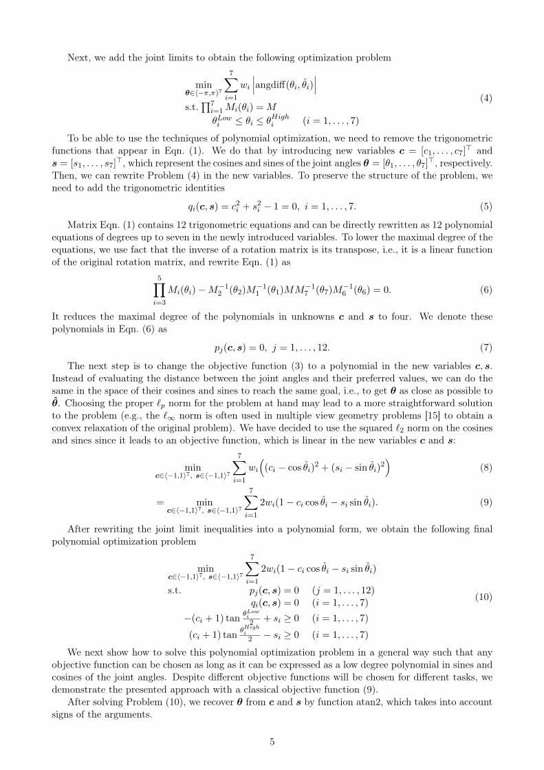
After rewriting the joint limit inequalities into a polynomial form, we obtain the following finalpolynomial optimization problem

minc∈〈−1,1〉7, s∈〈−1,1〉7

7∑i=1

2wi(1− ci cos θi − si sin θi)

s.t. pj(c, s) = 0 (j = 1, . . . , 12)qi(c, s) = 0 (i = 1, . . . , 7)

−(ci + 1) tanθLowi2 + si ≥ 0 (i = 1, . . . , 7)

(ci + 1) tanθHighi2 − si ≥ 0 (i = 1, . . . , 7)

(10)

We next show how to solve this polynomial optimization problem in a general way such that anyobjective function can be chosen as long as it can be expressed as a low degree polynomial in sines andcosines of the joint angles. Despite different objective functions will be chosen for different tasks, wedemonstrate the presented approach with a classical objective function (9).

After solving Problem (10), we recover θ from c and s by function atan2, which takes into accountsigns of the arguments.

5

4 Polynomial optimization

Here we describe the polynomial optimization methods we use to solve Problem (10).Polynomial optimization problems (POPs) are generally nonconvex, but they can be solved with

global optimality certificates with the help of convex optimization, as surveyed in [21]. The idea consistsof building a hierarchy of convex optimization problems of increasing size whose values converge to thevalue of the POP. The convergence proof is based on the results of real algebraic geometry, namely,on the representation of positive polynomials, or Positivstellensatz (PSatz for short). One of themost popular PSatz is due to Putinar [29], and it expresses a polynomial positive on a compact basicsemialgebraic set as a weighted sum of squares (SOS).

Finding this SOS representation amounts to solving a semidefinite programming (SDP) problem,a particular convex optimization problem that can be solved efficiently numerically with interior pointalgorithms. By increasing the degree of the SOS representation, we increase the size of the SDPproblem, thereby constructing a hierarchy of SDP problems. Dual to this polynomial positivity problemis the problem of characterizing the moments of measures supported on a compact basic semialgebraicset. This also admits an SDP formulation, called moment relaxations, yielding a dual hierarchy indexedby the so-called relaxation order.

The primal-dual hierarchy is called the moment-SOS hierarchy, or the Lasserre hierarchy since itwas first proposed in [20] in the context of POP with convergence and duality proofs. As the relaxationorder increases, the Lasserre hierarchy generates a monotone sequence of superoptimal bounds on theglobal optimum of a given POP. Eventually, the result on the moment problem can be used to certifythe exactness of the bound for the current relaxation order. This solves the original nonconvex POP atthe price of solving a relaxed convex SDP problem of typically (quite) bigger size than was the originalproblem. A Matlab package GloptiPoly [13] has been designed to construct the SDP problems in thehierarchy and solve them with a general-purpose SDP solver.

As observed in many applications, the main limitation of the Lasserre hierarchy (in its originalform) is its poor scalability as a function of the number of variables and the degree of the POP. Thisis balanced by the practical observation that, very often, global optimality is certified by the secondor third-order relaxation. As our experiments reveal, for the degree 4 POP studied in our paper,the third-order relaxation is out of reach of state-of-the-art SDP solvers. It becomes hence critical toinvestigate reformulation techniques to reduce the degree as much as possible. This is the topic of thenext section.

5 Symbolic reduction of the POP

Here we provide the description of the algebraic geometry technique we use to reduce the degree ofour POP problem to obtain a practical solving method. See [6] for algebraic-geometric notation andconcepts.

Let us assume that our POP is constrained by polynomial equations

f1 = · · · = fs = 0 (11)

of degree 4 in Q[x1, . . . , xn]. Observe that one can replace these polynomial equations in the POPformulation with any other set of polynomial equations

g1 = · · · = gt = 0 (12)

as long as both systems of equations have the same solution set. Natural candidates for gi’s arepolynomials in the ideal generated by f1, . . . , fs, i.e., in the set of algebraic combinations I = {

∑i qifi |

qi ∈ Q[x1, . . . , xn]}, which we denote as I = 〈f1, . . . , fs〉. It is clear that if all fi’s vanish simultaneouslyat a point, any polynomial g in this set I will vanish at that point.

The difficulty is how to understand the structure of this set and find a nice finite representationof it that would allow many algebraic operations (such as deciding whether a given polynomial lies inthis set). Solutions have been brought by symbolic computation, aka computer algebra, through thedevelopment of algorithms computing Gröbner bases, which were introduced by Buchberger, see [6].

6

These are finite sets, depending on a monomial ordering [6], which generate I as input equations do,but from which the whole structure of I can be read off.

Modern algorithms for computing Gröbner bases (F4 and F5 algorithms), which significantlyimproved by several orders of magnitude the state-of-the-art, were introduced next by J. C. Faugère[10, 11]. These latter algorithms bring a linear algebra approach to Gröbner bases computations. Inparticular, noticing that the intersection of I with the subset of polynomials in Q[x1, . . . , xn] of degree≤ d is a vector space of finite dimension is the key to reduce Gröbner bases computations to exactlinear algebra operations.

Hence, Gröbner bases provide bases of such vector spaces when one uses monomial orderings whichfilter monomials w.r.t. degree first. Finally, going back to our problem, a Gröbner basis computationallows us to discover if I contains degree 2 polynomials (and is generated by such quadrics).

While this is never the case when starting with a generic POP of degree 4, observe that there aremany relations between the coefficients of the degree 4 equations of our POP. Hence, we are not facinga generic situation here, and we will see further that a Gröbner basis computation provides a set ofquadrics that can replace our initial set of constraints. Note also that since Gröbner basis algorithmsrely on exact linear algebra, such a property holds for every generic instance of our POP if it holds for arandomly chosen one (the trace of the computation will always be the same, giving rise to polynomialsof degree ≤ 2).

6 Solving the IK problem

To solve the IK problem, we need to solve the optimization problem (10). First, we apply the imple-mentation GloptiPoly [13] of the method described in Section 4 directly on the Problem (10).

6.1 Direct application of polynomial solver

Since the original Problem (10) contains polynomials of degree four, we start with the first relaxationof order two. It means we substitute each monomial in the original 14 variables up to degree four bya new variable, and therefore the resulting SDP program will have 3060 variables.

Solving the first relaxation typically does not yield the solution for this parameterization of theproblem, and therefore it is required to go higher in the relaxation hierarchy. Unfortunately, therelaxation order three for a polynomial problem in 14 variables leads to an SDP problem in 38 760variables. Such a huge problem is still often solvable on contemporary computers, but it often takeshours to finish.

An example of using the GloptiPoly package [13] to solve a polynomial problem is shown in Listing 1.In the first part (lines 1–5), we create the unknowns c and s and load the kinematic parameters ofthe manipulator from a file. In the second part (lines 7–15), based on the kinematic parameters,function FKT generates the polynomials from the forward kinematics (Eqn. (7)), and we add to themthe trigonometric identities (Eqn. (5)). Then, function jointLimits, also based on the kinematicparameters of the manipulator, generates the inequalities coming from the joint limits. We define theobjective function f, which depends on the weights w and preferred values of the joint angles thHat.In the third part (lines 17–21), we configure GloptiPoly. We use the YALMIP toolbox [23] to definethe SDP problems and the MOSEK solver [2] to solve them. In the fourth part (lines 23–27), we useGloptiPoly to create the SDP problem from the POP for the given relaxation order relaxOrder andsolve it. In the last part (lines 29–34), we extract the solutions if we have succeeded in solving. Thevariable status is set to −1 if the POP is infeasible, to 0 if GloptiPoly can not certify the globality ofthe found solution, or to 1 if the found optimum was certified as global. If it is set to 1, then in thevariable obj is the value of the objective function evaluated on the solution, and we can recover thejoint angles from their sines and cosines by the function atan2.

6.2 Symbolic reduction

In the view of the previous paragraph, we aim at simplifying the original polynomial problem to beable to obtain solutions even for the relaxation of order two, which takes seconds to solve.

7

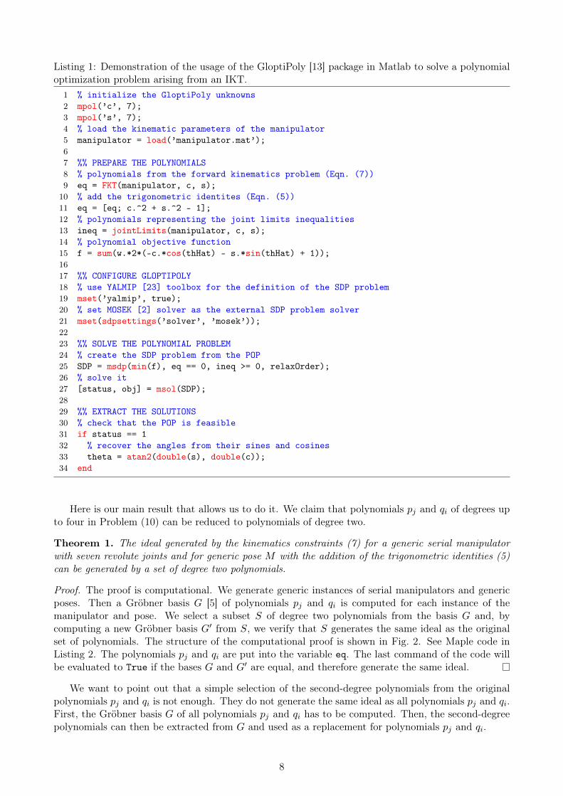
Listing 1: Demonstration of the usage of the GloptiPoly [13] package in Matlab to solve a polynomialoptimization problem arising from an IKT.

1 % initialize the GloptiPoly unknowns2 mpol(’c’, 7);3 mpol(’s’, 7);4 % load the kinematic parameters of the manipulator5 manipulator = load(’manipulator.mat’);67 %% PREPARE THE POLYNOMIALS8 % polynomials from the forward kinematics problem (Eqn. (7))9 eq = FKT(manipulator, c, s);

10 % add the trigonometric identites (Eqn. (5))11 eq = [eq; c.^2 + s.^2 - 1];12 % polynomials representing the joint limits inequalities13 ineq = jointLimits(manipulator, c, s);14 % polynomial objective function15 f = sum(w.*2*(-c.*cos(thHat) - s.*sin(thHat) + 1));1617 %% CONFIGURE GLOPTIPOLY18 % use YALMIP [23] toolbox for the definition of the SDP problem19 mset(’yalmip’, true);20 % set MOSEK [2] solver as the external SDP problem solver21 mset(sdpsettings(’solver’, ’mosek’));2223 %% SOLVE THE POLYNOMIAL PROBLEM24 % create the SDP problem from the POP25 SDP = msdp(min(f), eq == 0, ineq >= 0, relaxOrder);26 % solve it27 [status, obj] = msol(SDP);2829 %% EXTRACT THE SOLUTIONS30 % check that the POP is feasible31 if status == 132 % recover the angles from their sines and cosines33 theta = atan2(double(s), double(c));34 end

Here is our main result that allows us to do it. We claim that polynomials pj and qi of degrees upto four in Problem (10) can be reduced to polynomials of degree two.

Theorem 1. The ideal generated by the kinematics constraints (7) for a generic serial manipulatorwith seven revolute joints and for generic pose M with the addition of the trigonometric identities (5)can be generated by a set of degree two polynomials.

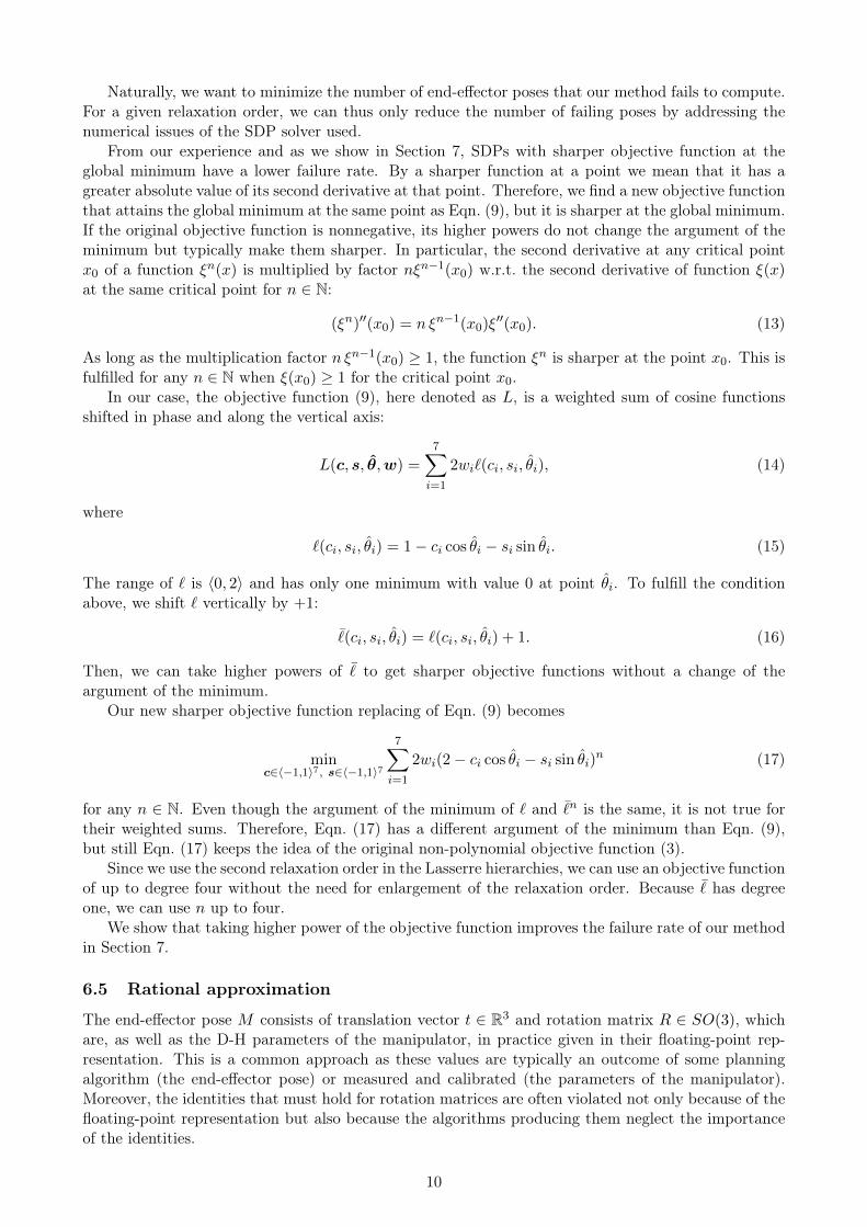
Proof. The proof is computational. We generate generic instances of serial manipulators and genericposes. Then a Gröbner basis G [5] of polynomials pj and qi is computed for each instance of themanipulator and pose. We select a subset S of degree two polynomials from the basis G and, bycomputing a new Gröbner basis G′ from S, we verify that S generates the same ideal as the originalset of polynomials. The structure of the computational proof is shown in Fig. 2. See Maple code inListing 2. The polynomials pj and qi are put into the variable eq. The last command of the code willbe evaluated to True if the bases G and G′ are equal, and therefore generate the same ideal.

We want to point out that a simple selection of the second-degree polynomials from the originalpolynomials pj and qi is not enough. They do not generate the same ideal as all polynomials pj and qi.First, the Gröbner basis G of all polynomials pj and qi has to be computed. Then, the second-degreepolynomials can then be extracted from G and used as a replacement for polynomials pj and qi.

8

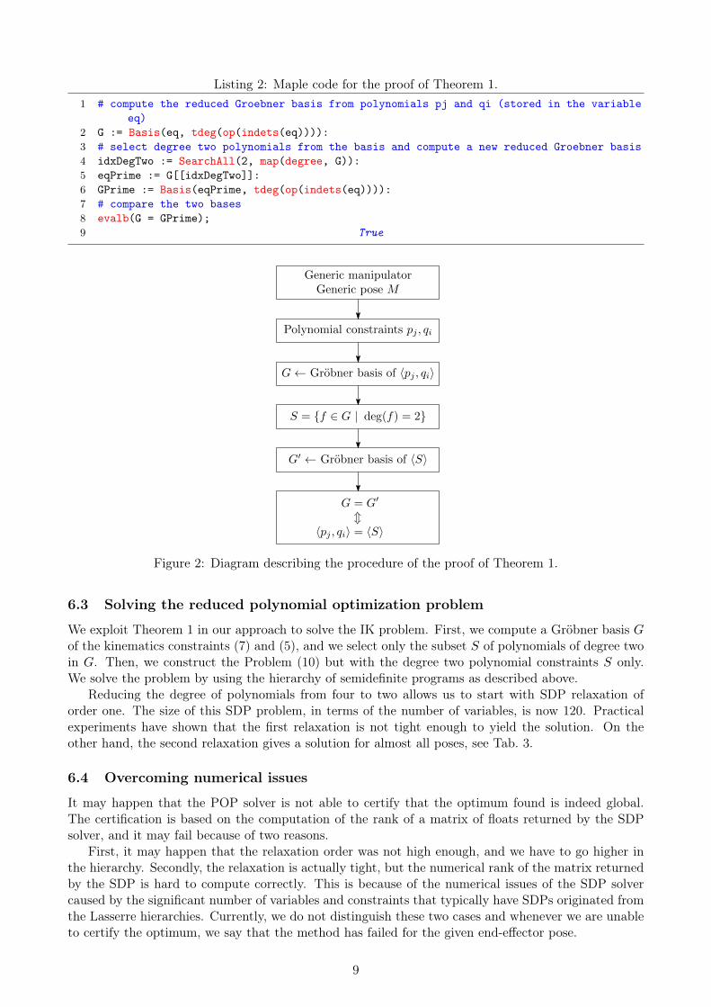
Listing 2: Maple code for the proof of Theorem 1.1 # compute the reduced Groebner basis from polynomials pj and qi (stored in the variable

eq)2 G := Basis(eq, tdeg(op(indets(eq)))):3 # select degree two polynomials from the basis and compute a new reduced Groebner basis4 idxDegTwo := SearchAll(2, map(degree, G)):5 eqPrime := G[[idxDegTwo]]:6 GPrime := Basis(eqPrime, tdeg(op(indets(eq)))):7 # compare the two bases8 evalb(G = GPrime);9 True

Generic manipulatorGeneric pose M

Polynomial constraints pj , qi

G← Grobner basis of 〈pj , qi〉

S = {f ∈ G | deg(f) = 2}

G′ ← Grobner basis of 〈S〉

G = G′

m〈pj , qi〉 = 〈S〉

Figure 2: Diagram describing the procedure of the proof of Theorem 1.

6.3 Solving the reduced polynomial optimization problem

We exploit Theorem 1 in our approach to solve the IK problem. First, we compute a Gröbner basis Gof the kinematics constraints (7) and (5), and we select only the subset S of polynomials of degree twoin G. Then, we construct the Problem (10) but with the degree two polynomial constraints S only.We solve the problem by using the hierarchy of semidefinite programs as described above.

Reducing the degree of polynomials from four to two allows us to start with SDP relaxation oforder one. The size of this SDP problem, in terms of the number of variables, is now 120. Practicalexperiments have shown that the first relaxation is not tight enough to yield the solution. On theother hand, the second relaxation gives a solution for almost all poses, see Tab. 3.

6.4 Overcoming numerical issues

It may happen that the POP solver is not able to certify that the optimum found is indeed global.The certification is based on the computation of the rank of a matrix of floats returned by the SDPsolver, and it may fail because of two reasons.

First, it may happen that the relaxation order was not high enough, and we have to go higher inthe hierarchy. Secondly, the relaxation is actually tight, but the numerical rank of the matrix returnedby the SDP is hard to compute correctly. This is because of the numerical issues of the SDP solvercaused by the significant number of variables and constraints that typically have SDPs originated fromthe Lasserre hierarchies. Currently, we do not distinguish these two cases and whenever we are unableto certify the optimum, we say that the method has failed for the given end-effector pose.

9

Naturally, we want to minimize the number of end-effector poses that our method fails to compute.For a given relaxation order, we can thus only reduce the number of failing poses by addressing thenumerical issues of the SDP solver used.

From our experience and as we show in Section 7, SDPs with sharper objective function at theglobal minimum have a lower failure rate. By a sharper function at a point we mean that it has agreater absolute value of its second derivative at that point. Therefore, we find a new objective functionthat attains the global minimum at the same point as Eqn. (9), but it is sharper at the global minimum.If the original objective function is nonnegative, its higher powers do not change the argument of theminimum but typically make them sharper. In particular, the second derivative at any critical pointx0 of a function ξn(x) is multiplied by factor nξn−1(x0) w.r.t. the second derivative of function ξ(x)at the same critical point for n ∈ N:

(ξn)′′(x0) = n ξn−1(x0)ξ′′(x0). (13)

As long as the multiplication factor n ξn−1(x0) ≥ 1, the function ξn is sharper at the point x0. This isfulfilled for any n ∈ N when ξ(x0) ≥ 1 for the critical point x0.

In our case, the objective function (9), here denoted as L, is a weighted sum of cosine functionsshifted in phase and along the vertical axis:

L(c, s, θ,w) =7∑i=1

2wi`(ci, si, θi), (14)

where

`(ci, si, θi) = 1− ci cos θi − si sin θi. (15)

The range of ` is 〈0, 2〉 and has only one minimum with value 0 at point θi. To fulfill the conditionabove, we shift ` vertically by +1:

¯(ci, si, θi) = `(ci, si, θi) + 1. (16)

Then, we can take higher powers of ¯ to get sharper objective functions without a change of theargument of the minimum.

Our new sharper objective function replacing of Eqn. (9) becomes

minc∈〈−1,1〉7, s∈〈−1,1〉7

7∑i=1

2wi(2− ci cos θi − si sin θi)n (17)

for any n ∈ N. Even though the argument of the minimum of ` and ¯n is the same, it is not true fortheir weighted sums. Therefore, Eqn. (17) has a different argument of the minimum than Eqn. (9),but still Eqn. (17) keeps the idea of the original non-polynomial objective function (3).

Since we use the second relaxation order in the Lasserre hierarchies, we can use an objective functionof up to degree four without the need for enlargement of the relaxation order. Because ¯ has degreeone, we can use n up to four.

We show that taking higher power of the objective function improves the failure rate of our methodin Section 7.

6.5 Rational approximation

The end-effector pose M consists of translation vector t ∈ R3 and rotation matrix R ∈ SO(3), whichare, as well as the D-H parameters of the manipulator, in practice given in their floating-point rep-resentation. This is a common approach as these values are typically an outcome of some planningalgorithm (the end-effector pose) or measured and calibrated (the parameters of the manipulator).Moreover, the identities that must hold for rotation matrices are often violated not only because of thefloating-point representation but also because the algorithms producing them neglect the importanceof the identities.

10

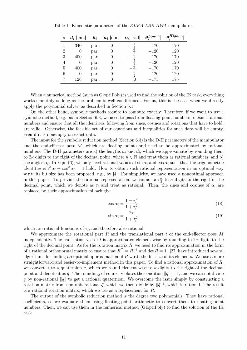
Table 1: Kinematic parameters of the KUKA LBR IIWA manipulator.

i di [mm] θi ai [mm] αi [rad] θLowi [°] θHighi [°]

1 340 par. 0 −π2 −170 170

2 0 par. 0 π2 −120 120

3 400 par. 0 −π2 −170 170

4 0 par. 0 π2 −120 120

5 400 par. 0 −π2 −170 170

6 0 par. 0 π2 −120 120

7 126 par. 0 0 −175 175

When a numerical method (such as GloptiPoly) is used to find the solution of the IK task, everythingworks smoothly as long as the problem is well-conditioned. For us, this is the case when we directlyapply the polynomial solver, as described in Section 6.1.

On the other hand, symbolic methods require to compute exactly. Therefore, if we want to use asymbolic method, e.g., as in Section 6.3, we need to pass from floating-point numbers to exact rationalnumbers and ensure that all the identities, following from sines, cosines and rotations that have to hold,are valid. Otherwise, the feasible set of our equations and inequalities for such data will be empty,even if it is nonempty on exact data.

The input for the symbolic reduction method (Section 6.3) is the D-H parameters of the manipulatorand the end-effector pose M , which are floating points and need to be approximated by rationalnumbers. The D-H parameters are a) the lengths ai and di, which we approximate by rounding themto 2κ digits to the right of the decimal point, where κ ∈ N and treat them as rational numbers, and b)the angles αi. In Eqn. (6), we only need rational values of sinαi and cosαi such that the trigonometricidentities sin2 αi + cos2 αi = 1 hold. How to obtain such rational representation in an optimal wayw.r.t. its bit size has been proposed, e.g., by [4]. For simplicity, we have used a nonoptimal approachin this paper. To provide the rational representation, we round tan α

2 to κ digits to the right of thedecimal point, which we denote as τi and treat as rational. Then, the sines and cosines of αi arereplaced by their approximation followingly:

cosαi =1− τ2i1 + τ2i

, (18)

sinαi =2τ

1 + τ2i, (19)

which are rational functions of τi, and therefore also rational.We approximate the rotational part R and the translational part t of the end-effector pose M

independently. The translation vector t is approximated element-wise by rounding to 2κ digits to theright of the decimal point. As for the rotation matrix R, we need to find its approximation in the formof a rational orthonormal matrix to ensure that R> = R−1 and detR = 1. [27] have introduced severalalgorithms for finding an optimal approximation of R w.r.t. the bit size of its elements. We use a morestraightforward and easier-to-implement method in this paper. To find a rational approximation of R,we convert it to a quaternion q, which we round element-wise to κ digits to the right of the decimalpoint and denote it as q. The rounding, of course, violates the condition ‖q‖ = 1, and we can not divideq by non-rational ‖q‖ to get a rational quaternion. We overcome the issue simply by constructing arotation matrix from non-unit rational q, which we then divide by ‖q‖2, which is rational. The resultis a rational rotation matrix, which we use as a replacement for R.

The output of the symbolic reduction method is the degree two polynomials. They have rationalcoefficients, so we evaluate them using floating-point arithmetic to convert them to floating-pointnumbers. Then, we can use them in the numerical method (GloptiPoly) to find the solution of the IKtask.

11

-200 0 200 4000

0

200

400

600

800

1000

1200

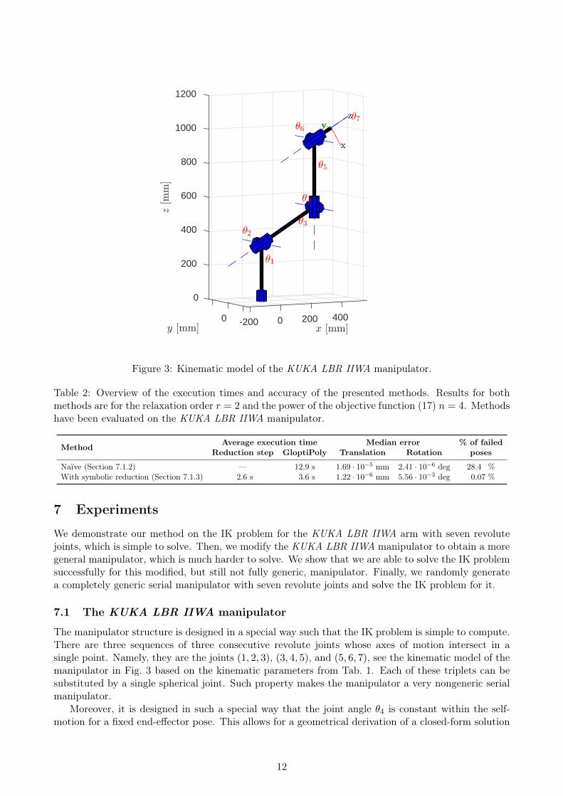
Figure 3: Kinematic model of the KUKA LBR IIWA manipulator.

Table 2: Overview of the execution times and accuracy of the presented methods. Results for bothmethods are for the relaxation order r = 2 and the power of the objective function (17) n = 4. Methodshave been evaluated on the KUKA LBR IIWA manipulator.

Method Average execution time Median error % of failedReduction step GloptiPoly Translation Rotation poses

Naïve (Section 7.1.2) — 12.9 s 1.69 · 10−5 mm 2.41 · 10−6 deg 28.4 %With symbolic reduction (Section 7.1.3) 2.6 s 3.6 s 1.22 · 10−6 mm 5.56 · 10−3 deg 0.07 %

7 Experiments

We demonstrate our method on the IK problem for the KUKA LBR IIWA arm with seven revolutejoints, which is simple to solve. Then, we modify the KUKA LBR IIWA manipulator to obtain a moregeneral manipulator, which is much harder to solve. We show that we are able to solve the IK problemsuccessfully for this modified, but still not fully generic, manipulator. Finally, we randomly generatea completely generic serial manipulator with seven revolute joints and solve the IK problem for it.

7.1 The KUKA LBR IIWA manipulator

The manipulator structure is designed in a special way such that the IK problem is simple to compute.There are three sequences of three consecutive revolute joints whose axes of motion intersect in asingle point. Namely, they are the joints (1, 2, 3), (3, 4, 5), and (5, 6, 7), see the kinematic model of themanipulator in Fig. 3 based on the kinematic parameters from Tab. 1. Each of these triplets can besubstituted by a single spherical joint. Such property makes the manipulator a very nongeneric serialmanipulator.

Moreover, it is designed in such a special way that the joint angle θ4 is constant within the self-motion for a fixed end-effector pose. This allows for a geometrical derivation of a closed-form solution

12

-800-600-400-200 0 200 400 600 800-800-600-400-2000200400600800

01002003004005006007008009001000

x [mm]

y [mm]

z [mm]

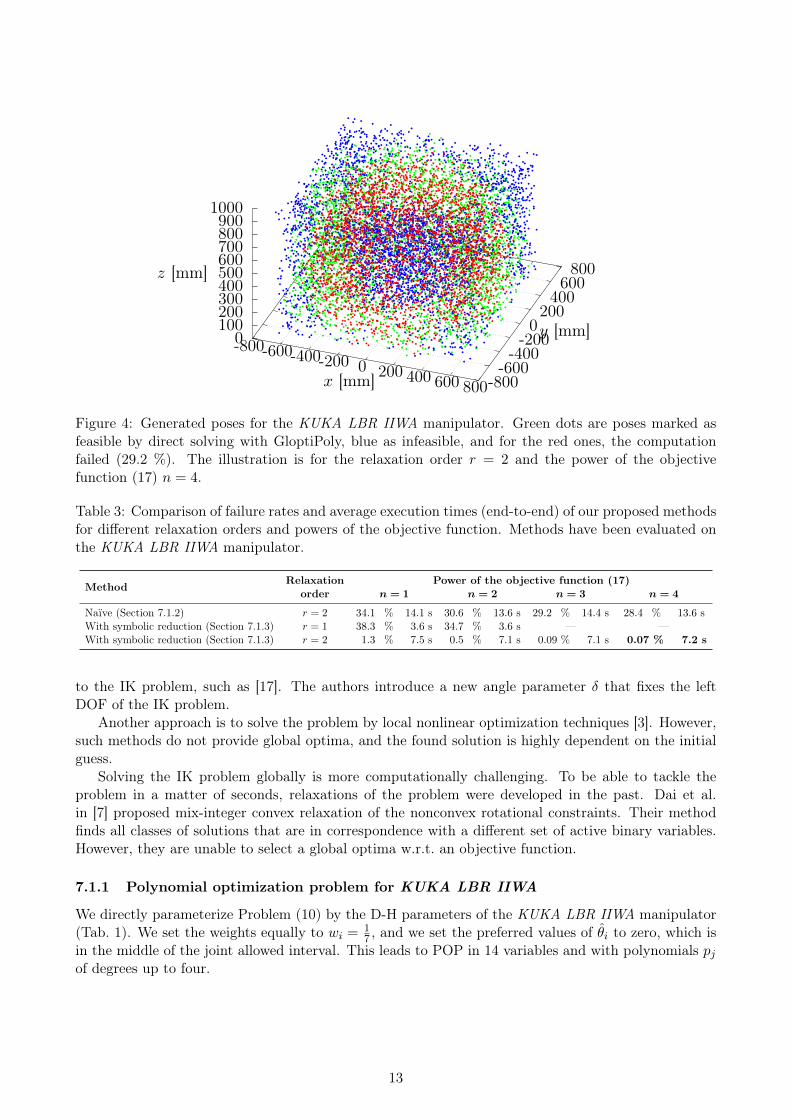
Figure 4: Generated poses for the KUKA LBR IIWA manipulator. Green dots are poses marked asfeasible by direct solving with GloptiPoly, blue as infeasible, and for the red ones, the computationfailed (29.2 %). The illustration is for the relaxation order r = 2 and the power of the objectivefunction (17) n = 4.

Table 3: Comparison of failure rates and average execution times (end-to-end) of our proposed methodsfor different relaxation orders and powers of the objective function. Methods have been evaluated onthe KUKA LBR IIWA manipulator.

Method Relaxation Power of the objective function (17)order n = 1 n = 2 n = 3 n = 4

Naïve (Section 7.1.2) r = 2 34.1 % 14.1 s 30.6 % 13.6 s 29.2 % 14.4 s 28.4 % 13.6 sWith symbolic reduction (Section 7.1.3) r = 1 38.3 % 3.6 s 34.7 % 3.6 s — —With symbolic reduction (Section 7.1.3) r = 2 1.3 % 7.5 s 0.5 % 7.1 s 0.09 % 7.1 s 0.07 % 7.2 s

to the IK problem, such as [17]. The authors introduce a new angle parameter δ that fixes the leftDOF of the IK problem.

Another approach is to solve the problem by local nonlinear optimization techniques [3]. However,such methods do not provide global optima, and the found solution is highly dependent on the initialguess.

Solving the IK problem globally is more computationally challenging. To be able to tackle theproblem in a matter of seconds, relaxations of the problem were developed in the past. Dai et al.in [7] proposed mix-integer convex relaxation of the nonconvex rotational constraints. Their methodfinds all classes of solutions that are in correspondence with a different set of active binary variables.However, they are unable to select a global optima w.r.t. an objective function.

7.1.1 Polynomial optimization problem for KUKA LBR IIWA

We directly parameterize Problem (10) by the D-H parameters of the KUKA LBR IIWA manipulator(Tab. 1). We set the weights equally to wi = 1

7 , and we set the preferred values of θi to zero, which isin the middle of the joint allowed interval. This leads to POP in 14 variables and with polynomials pjof degrees up to four.

13

-800-600-400-200 0 200 400 600 800-800-600-400-2000200400600800

01002003004005006007008009001000

x [mm]

y [mm]

z [mm]

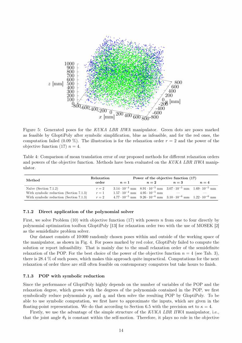
Figure 5: Generated poses for the KUKA LBR IIWA manipulator. Green dots are poses markedas feasible by GloptiPoly after symbolic simplification, blue as infeasible, and for the red ones, thecomputation failed (0.09 %). The illustration is for the relaxation order r = 2 and the power of theobjective function (17) n = 4.

Table 4: Comparison of mean translation error of our proposed methods for different relaxation ordersand powers of the objective function. Methods have been evaluated on the KUKA LBR IIWA manip-ulator.

Method Relaxation Power of the objective function (17)order n = 1 n = 2 n = 3 n = 4

Naïve (Section 7.1.2) r = 2 3.14 · 10−4 mm 8.91 · 10−5 mm 3.07 · 10−5 mm 1.69 · 10−5 mmWith symbolic reduction (Section 7.1.3) r = 1 1.57 · 10−4 mm 4.95 · 10−5 mm — —With symbolic reduction (Section 7.1.3) r = 2 4.77 · 10−5 mm 9.26 · 10−6 mm 3.10 · 10−6 mm 1.22 · 10−6 mm

7.1.2 Direct application of the polynomial solver

First, we solve Problem (10) with objective function (17) with powers n from one to four directly bypolynomial optimization toolbox GloptiPoly [13] for relaxation order two with the use of MOSEK [2]as the semidefinite problem solver.

Our dataset consists of 10 000 randomly chosen poses within and outside of the working space ofthe manipulator, as shown in Fig. 4. For poses marked by red color, GloptiPoly failed to compute thesolution or report infeasibility. That is mainly due to the small relaxation order of the semidefiniterelaxation of the POP. For the best choice of the power of the objective function n = 4 (see Tab. 3),there is 28.4 % of such poses, which makes this approach quite impractical. Computations for the nextrelaxation of order three are still often feasible on contemporary computers but take hours to finish.

7.1.3 POP with symbolic reduction

Since the performance of GloptiPoly highly depends on the number of variables of the POP and therelaxation degree, which grows with the degrees of the polynomials contained in the POP, we firstsymbolically reduce polynomials pj and qi and then solve the resulting POP by GloptiPoly. To beable to use symbolic computation, we first have to approximate the inputs, which are given in thefloating-point representation. We do that according to Section 6.5 with the precision set to κ = 4.

Firstly, we use the advantage of the simple structure of the KUKA LBR IIWA manipulator, i.e.,that the joint angle θ4 is constant within the self-motion. Therefore, it plays no role in the objective

14

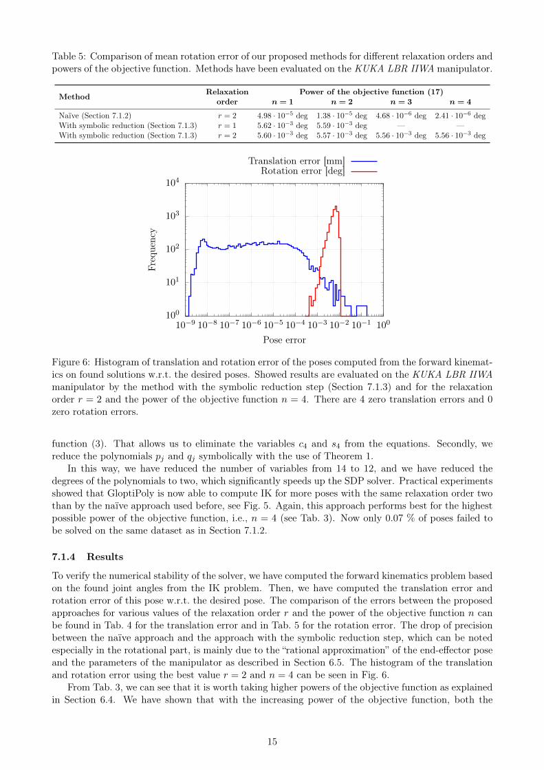
Table 5: Comparison of mean rotation error of our proposed methods for different relaxation orders andpowers of the objective function. Methods have been evaluated on the KUKA LBR IIWA manipulator.

Method Relaxation Power of the objective function (17)order n = 1 n = 2 n = 3 n = 4

Naïve (Section 7.1.2) r = 2 4.98 · 10−5 deg 1.38 · 10−5 deg 4.68 · 10−6 deg 2.41 · 10−6 degWith symbolic reduction (Section 7.1.3) r = 1 5.62 · 10−3 deg 5.59 · 10−3 deg — —With symbolic reduction (Section 7.1.3) r = 2 5.60 · 10−3 deg 5.57 · 10−3 deg 5.56 · 10−3 deg 5.56 · 10−3 deg

100

101

102

103

104

10−9 10−8 10−7 10−6 10−5 10−4 10−3 10−2 10−1 100

Frequency

Pose error

Translation error [mm]Rotation error [deg]

Figure 6: Histogram of translation and rotation error of the poses computed from the forward kinemat-ics on found solutions w.r.t. the desired poses. Showed results are evaluated on the KUKA LBR IIWAmanipulator by the method with the symbolic reduction step (Section 7.1.3) and for the relaxationorder r = 2 and the power of the objective function n = 4. There are 4 zero translation errors and 0zero rotation errors.

function (3). That allows us to eliminate the variables c4 and s4 from the equations. Secondly, wereduce the polynomials pj and qj symbolically with the use of Theorem 1.

In this way, we have reduced the number of variables from 14 to 12, and we have reduced thedegrees of the polynomials to two, which significantly speeds up the SDP solver. Practical experimentsshowed that GloptiPoly is now able to compute IK for more poses with the same relaxation order twothan by the naïve approach used before, see Fig. 5. Again, this approach performs best for the highestpossible power of the objective function, i.e., n = 4 (see Tab. 3). Now only 0.07 % of poses failed tobe solved on the same dataset as in Section 7.1.2.

7.1.4 Results

To verify the numerical stability of the solver, we have computed the forward kinematics problem basedon the found joint angles from the IK problem. Then, we have computed the translation error androtation error of this pose w.r.t. the desired pose. The comparison of the errors between the proposedapproaches for various values of the relaxation order r and the power of the objective function n canbe found in Tab. 4 for the translation error and in Tab. 5 for the rotation error. The drop of precisionbetween the naïve approach and the approach with the symbolic reduction step, which can be notedespecially in the rotational part, is mainly due to the “rational approximation” of the end-effector poseand the parameters of the manipulator as described in Section 6.5. The histogram of the translationand rotation error using the best value r = 2 and n = 4 can be seen in Fig. 6.

From Tab. 3, we can see that it is worth taking higher powers of the objective function as explainedin Section 6.4. We have shown that with the increasing power of the objective function, both the

15

100

101

102

103

104

2 4 6 8 10

Frequency

GloptiPoly execution time [s]2 2.2 2.4 2.6 2.8 3 3.2 3.4

Maple execution time [s]

Feasible posesInfeasible poses

Poses failed to compute

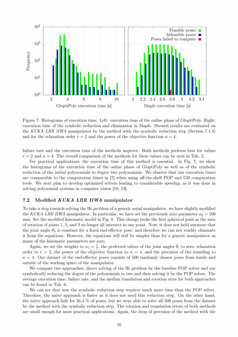
Figure 7: Histograms of execution time. Left: execution time of the online phase of GloptiPoly. Right:execution time of the symbolic reduction and elimination in Maple. Showed results are evaluated onthe KUKA LBR IIWA manipulator by the method with the symbolic reduction step (Section 7.1.3)and for the relaxation order r = 2 and the power of the objective function n = 4.

failure rate and the execution time of the methods improve. Both methods perform best for valuesr = 2 and n = 4. The overall comparison of the methods for these values can be seen in Tab. 2.

For practical applications, the execution time of this method is essential. In Fig. 7, we showthe histograms of the execution time of the online phase of GloptiPoly as well as of the symbolicreduction of the initial polynomials to degree two polynomials. We observe that our execution timesare comparable to the computation times in [7] when using off-the-shelf POP and GB computationtools. We next plan to develop optimized solvers leading to considerable speedup, as it was done insolving polynomial systems in computer vision [18, 19].

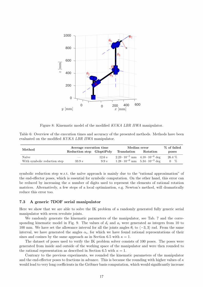
7.2 Modified KUKA LBR IIWA manipulator

To take a step towards solving the IK problem of a generic serial manipulator, we have slightly modifiedthe KUKA LBR IIWA manipulator. In particular, we have set the previously zero parameter a2 = 100mm. See the modified kinematic model in Fig. 8. This change broke the first spherical joint as the axesof rotation of joints 1, 2, and 3 no longer all intersect in one point. Now, it does not hold anymore thatthe joint angle θ4 is constant for a fixed end-effector pose, and therefore we can not readily eliminateit from the equations. However, the equations will still be simpler than for a generic manipulator asmany of the kinematic parameters are zero.

Again, we set the weights to wi = 17 , the preferred values of the joint angles θi to zero, relaxation

order to r = 2, the power of the objective function to n = 4, and the precision of the rounding toκ = 4. Our dataset of the end-effector poses consists of 500 randomly chosen poses from inside andoutside of the working space of the manipulator.

We compare two approaches: direct solving of the IK problem by the baseline POP solver and oursymbolically reducing the degree of the polynomials to two and then solving it by the POP solver. Theaverage execution time, failure rate, and the median translation and rotation error for both approachescan be found in Tab. 6.

We can see that now the symbolic reduction step requires much more time than the POP solver.Therefore, the naïve approach is faster as it does not need this reduction step. On the other hand,the naïve approach fails for 26.4 % of poses, but we were able to solve all 500 poses from the datasetby the method with the symbolic reduction step. The rotation and translation errors of both methodsare small enough for most practical applications. Again, the drop of precision of the method with the

16

0 200 400 6000

0

200

400

600

800

1000

Figure 8: Kinematic model of the modified KUKA LBR IIWA manipulator.

Table 6: Overview of the execution times and accuracy of the presented methods. Methods have beenevaluated on the modified KUKA LBR IIWA manipulator.

Method Average execution time Median error % of failedReduction step GloptiPoly Translation Rotation poses

Naïve — 12.6 s 2.23 · 10−5 mm 4.18 · 10−6 deg 26.4 %With symbolic reduction step 33.9 s 9.9 s 1.28 · 10−6 mm 5.34 · 10−3 deg 0 %

symbolic reduction step w.r.t. the naïve approach is mainly due to the “rational approximation” ofthe end-effector poses, which is essential for symbolic computation. On the other hand, this error canbe reduced by increasing the κ number of digits used to represent the elements of rational rotationmatrices. Alternatively, a few steps of a local optimization, e.g. Newton’s method, will dramaticallyreduce this error too.

7.3 A generic 7DOF serial manipulator

Here we show that we are able to solve the IK problem of a randomly generated fully generic serialmanipulator with seven revolute joints.

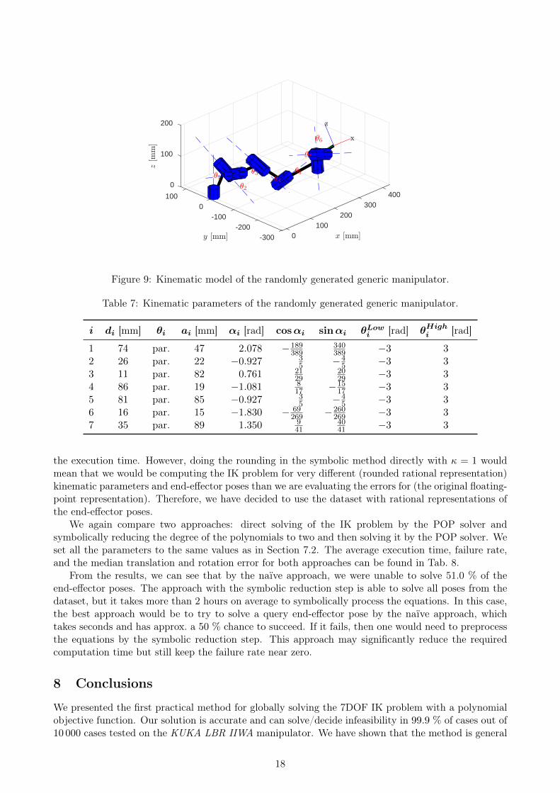
We randomly generate the kinematic parameters of the manipulator, see Tab. 7 and the corre-sponding kinematic model in Fig. 9. The values of di and ai were generated as integers from 10 to100 mm. We have set the allowance interval for all the joints angles θi to 〈−3, 3〉 rad. From the sameinterval, we have generated the angles αi, for which we have found rational representations of theirsines and cosines by the same approach as in Section 6.5 with κ = 1.

The dataset of poses used to verify the IK problem solver consists of 100 poses. The poses weregenerated from inside and outside of the working space of the manipulator and were then rounded tothe rational representation as described in Section 6.5 with κ = 1.

Contrary to the previous experiments, we rounded the kinematic parameters of the manipulatorand the end-effector poses to fractions in advance. This is because the rounding with higher values of κwould lead to very long coefficients in the Gröbner basis computation, which would significantly increase

17

0100

200300

400

-300-200

-1000

100

0

100

200

Figure 9: Kinematic model of the randomly generated generic manipulator.

Table 7: Kinematic parameters of the randomly generated generic manipulator.

i di [mm] θi ai [mm] αi [rad] cosαi sinαi θLowi [rad] θHighi [rad]

1 74 par. 47 2.078 −189389

340389 −3 3

2 26 par. 22 −0.927 35 −4

5 −3 33 11 par. 82 0.761 21

292029 −3 3

4 86 par. 19 −1.081 817 −15

17 −3 35 81 par. 85 −0.927 3

5 −45 −3 3

6 16 par. 15 −1.830 − 69269 −260

269 −3 37 35 par. 89 1.350 9

414041 −3 3

the execution time. However, doing the rounding in the symbolic method directly with κ = 1 wouldmean that we would be computing the IK problem for very different (rounded rational representation)kinematic parameters and end-effector poses than we are evaluating the errors for (the original floating-point representation). Therefore, we have decided to use the dataset with rational representations ofthe end-effector poses.

We again compare two approaches: direct solving of the IK problem by the POP solver andsymbolically reducing the degree of the polynomials to two and then solving it by the POP solver. Weset all the parameters to the same values as in Section 7.2. The average execution time, failure rate,and the median translation and rotation error for both approaches can be found in Tab. 8.

From the results, we can see that by the naïve approach, we were unable to solve 51.0 % of theend-effector poses. The approach with the symbolic reduction step is able to solve all poses from thedataset, but it takes more than 2 hours on average to symbolically process the equations. In this case,the best approach would be to try to solve a query end-effector pose by the naïve approach, whichtakes seconds and has approx. a 50 % chance to succeed. If it fails, then one would need to preprocessthe equations by the symbolic reduction step. This approach may significantly reduce the requiredcomputation time but still keep the failure rate near zero.

8 Conclusions

We presented the first practical method for globally solving the 7DOF IK problem with a polynomialobjective function. Our solution is accurate and can solve/decide infeasibility in 99.9 % of cases out of10 000 cases tested on the KUKA LBR IIWA manipulator. We have shown that the method is general

18

Table 8: Overview of the execution times and accuracy of the presented methods. Methods have beenevaluated on the randomly generated generic manipulator.

Method Average execution time Median error % of failedReduction step GloptiPoly Translation Rotation poses

Naïve — 14.0 s 1.02 · 10−6 mm 0 deg 51.0 %With symbolic reduction step 7331 s 11.0 s 9.62 · 10−8 mm 0 deg 0 %

and therefore can be used to solve the IK problem of a generic 7DOF serial revolute manipulator. Thecode is open-sourced at https://github.com/PavelTrutman/Global-7DOF-IKT.

For future work, we consider two interesting directions. First, in the case that the POP constraintsare incompatible (i.e., the feasible set of admissible parameters is empty), it would be desirable toreturn a certificate of infeasibility. This certificate can be either numerical (obtained by solving themoment-SOS hierarchy with an SDP solver) or symbolic (obtained by the Gröbner basis method).It can be obtained, e.g., by computing an SOS representation for the polynomial −1 (or any othernegative polynomial) on the quadratic module corresponding to the feasible set. See, e.g., [16] in thespecific case of certifying emptiness of spectrahedra (SDP feasibility sets).

Secondly, it would be interesting to exploit the specific structure of the POP studied in this paperto prove (maybe under some assumptions on the data) the exactness of the first or the second SDPrelaxation in the moment-SOS hierarchy, i.e., that solving this relaxation always solves the originalPOP. For Euclidean distance POP arising in computer vision, this was achieved in [1] by arguing onthe curvature properties of the Lagrangian and its SOS representation in the quadratic module.

Acknowledgments

P. Trutman and T. Pajdla were supported by the EU Structural and Investment Funds, OperationalPrograme Research, Development and Education under the project IMPACT (reg. no. CZ.02.1.01/0.0/-0.0/15_003/0000468) and Grant Agency of the CTU Prague project SGS19/173/OHK3/3T/13. Di-dier Henrion and Mohab Safey El Din are supported by the European Union’s Horizon2020 researchand innovation programme under the Marie Skłodowska-Curie grant agreement N°813211 (POEMA).Mohab Safey El Din is supported by the ANR grants ANR-18-CE33-0011 Sesame, ANR-19-CE40-0018De Rerum Natura, ANR-19-CE48-0015 ECARP, and the CAMiSAdo PGMO project.

References

[1] Chris Aholt, Sameer Agarwal, and Rekha Thomas. A qcqp approach to triangulation. In EuropeanConference on Computer Vision, pages 654–667. Springer, 2012.

[2] MOSEK ApS. The MOSEK optimization toolbox for MATLAB manual. Version 8.0., 2016.

[3] Samuel R Buss. Introduction to inverse kinematics with jacobian transpose, pseudoinverse anddamped least squares methods. IEEE Journal of Robotics and Automation, 17(1-19):16, 2004.

[4] John Canny, Bruce Donald, and Eugene K Ressler. A rational rotation method for robust geo-metric algorithms. In Proceedings of the eighth annual symposium on Computational geometry,pages 251–260, 1992.

[5] David Cox, John Little, and Donal OShea. Ideals, varieties, and algorithms: an introduction tocomputational algebraic geometry and commutative algebra. Springer Science & Business Media,2013.

[6] David A. Cox, John Little, and Donald O’Shea. Ideals, Varieties, and Algorithms: An Introductionto Computational Algebraic Geometry and Commutative Algebra. Springer, 2015.

19

[7] Hongkai Dai, Gregory Izatt, and Russ Tedrake. Global inverse kinematics via mixed-integer convexoptimization. The International Journal of Robotics Research, page 0278364919846512, 2017.

[8] Hongkai Dai, Andrés Valenzuela, and Russ Tedrake. Whole-body motion planning with centroidaldynamics and full kinematics. In 2014 IEEE-RAS International Conference on Humanoid Robots,pages 295–302. IEEE, 2014.

[9] Rosen Diankov. Automated Construction of Robotic Manipulation Programs. PhD thesis, Pitts-burgh, PA, USA, 2010. AAI3448143.

[10] Jean-Charles Faugère. A new efficient algorithm for computing gröbner bases (f4). Journal ofPure and Applied Algebra, 139(1):61 – 88, 1999.

[11] Jean Charles Faugère. A new efficient algorithm for computing gröbner bases without reductionto zero (f5). In Proceedings of the 2002 International Symposium on Symbolic and AlgebraicComputation, ISSAC ’02, pages 75–83, New York, NY, USA, 2002. ACM.

[12] Richard S Hartenberg and Jacques Denavit. A kinematic notation for lower pair mechanismsbased on matrices. Journal of applied mechanics, 77(2):215–221, 1955.

[13] Didier Henrion and Jean-Bernard Lasserre. Gloptipoly: Global optimization over polynomialswith matlab and sedumi. ACM Transactions on Mathematical Software (TOMS), 29(2):165–194,2003.

[14] Reza Jazar. Theory of Applied Robotics: Kinematics, Dynamics, and Control. Springer, 2007.

[15] Fredrik Kahl and Richard Hartley. Multiple-view geometry under the L∞-norm. IEEE Transac-tions on Pattern Analysis and Machine Intelligence, 30(9):1603–1617, 2008.

[16] Igor Klep and Markus Schweighofer. An exact duality theory for semidefinite programming basedon sums of squares. Mathematics of Operations Research, 38(3):569–590, 2013.

[17] I Kuhlemann, A Schweikard, P Jauer, and F Ernst. Robust inverse kinematics by configurationcontrol for redundant manipulators with seven dof. In 2016 2nd International Conference onControl, Automation and Robotics (ICCAR), pages 49–55. IEEE, 2016.

[18] Zuzana Kukelova, Martin Bujnak, and Tomas Pajdla. Automatic generator of minimal problemsolvers. In European Conference on Computer Vision (ECCV), pages 302–315. Springer, 2008.

[19] Viktor Larsson, Magnus Oskarsson, Kalle Åström, Alge Wallis, Zuzana Kukelova, and TomásPajdla. Beyond grobner bases: Basis selection for minimal solvers. In 2018 IEEE Conference onComputer Vision and Pattern Recognition, CVPR 2018, Salt Lake City, UT, USA, June 18-22,2018, pages 3945–3954, 2018.

[20] Jean Bernard Lasserre. Global optimization with polynomials and the problem of moments. SIAMJournal on optimization, 11(3):796–817, 2001.

[21] Jean Bernard Lasserre. An introduction to polynomial and semi-algebraic optimization, volume 52.Cambridge University Press, 2015.

[22] Daniel Lazard. Generalized stewart platform: How to compute with rigid motions. 1993.

[23] Johan Löfberg. YALMIP : A toolbox for modeling and optimization in MATLAB. In Proceedingsof the CACSD Conference, Taipei, Taiwan, 2004.

[24] Dinesh Manocha and John F. Canny. Efficient inverse kinematics for general 6r manipulators.IEEE Trans. Robotics and Automation, 10(5):648–657, 1994.

[25] Filip Marić, Matthew Giamou, Soroush Khoubyarian, Ivan Petrović, and Jonathan Kelly. Inversekinematics for serial kinematic chains via sum of squares optimization. In 2020 IEEE InternationalConference on Robotics and Automation (ICRA), pages 7101–7107. IEEE, 2020.

20

[26] Ernst W Mayr and Albert R Meyer. The complexity of the word problems for commutativesemigroups and polynomial ideals. Advances in Mathematics, 46(3):305 – 329, 1982.

[27] Victor J Milenkovic and Veljko Milenkovic. Rational orthogonal approximations to orthogonalmatrices. Computational Geometry, 7(1-2):25–35, 1997.

[28] Ugo Pattacini, Francesco Nori, Lorenzo Natale, Giorgio Metta, and Giulio Sandini. An exper-imental evaluation of a novel minimum-jerk cartesian controller for humanoid robots. In 2010IEEE/RSJ international conference on intelligent robots and systems, pages 1668–1674. IEEE,2010.

[29] Mihai Putinar. Positive polynomials on compact semi-algebraic sets. Indiana University Mathe-matics Journal, 42(3):969–984, 1993.

[30] Manasa Raghavan and Bernard Roth. Inverse kinematics of the general 6r manipulator and relatedlinkages. 1993.

[31] Manasa Raghavan and Bernard Roth. Solving polynomial systems for the kinematic analysis andsynthesis of mechanisms and robot manipulators. 1995.

[32] Madhusudan Raghaven and Bernard Roth. Kinematic analysis of the 6r manipulator of generalgeometry. In The Fifth International Symposium on Robotics Research, pages 263–269, Cambridge,MA, USA, 1990. MIT Press.

[33] J.E. Shigley and J.J. Uicker. Theory of machines and mechanisms. McGraw-Hill series in me-chanical engineering. McGraw-Hill, 1980.

[34] Charles W. Wampler, Alexander P. Morgan, and Andrew J. Sommese. Numerical continuationmethods for solving polynomial systems arising in kinematics. 1990.

21