1

Transformation of Optimal Centralized Controllers IntoNear-Globally Optimal Static Distributed Controllers

Salar Fattahi∗, Ghazal Fazelnia+, and Javad Lavaei∗∗Department of Industrial Engineering and Operations Research, University of California, Berkeley

+Department of Electrical Engineering, Columbia University

Abstract—This paper is concerned with the optimal dis-tributed control problem for linear discrete-time deterministicand stochastic systems. The objective is to design a stabilizingstatic distributed controller whose performance is close to thatof the optimal centralized controller. To this end, a necessaryand sufficient condition is derived to guarantee the existenceof a distributed controller that generates the same input andstate trajectories as the optimal centralized controller for a givendeterministic system. This condition is then translated into a con-vex optimization problem. Subsequently, a regularization termis incorporated into the objective of the proposed optimizationproblem to indirectly account for the stability of the distributedcontrol system. The designed optimization problem has a closed-form solution (explicit formula) and can be efficiently solvedfor large-scale systems that require low computational efforts.Furthermore, strong theoretical lower bounds are derived onthe optimality guarantee of the designed distributed controllerin the case where the proposed conditions do not hold. Weshow that if the optimal objective value of the proposed convexprogram is sufficiently small, the designed controller is stabilizingand nearly globally optimal. The results are then extended tostochastic systems that are subject to input disturbance andmeasurement noise. By building upon the developed methodology,we partially address some long-standing problems, such asfinding the minimum number of free elements required in thedistributed controller under design to achieve a performanceclose to the optimal centralized one. Numerical results on a powernetwork and several random systems are reported to demonstratethe efficacy of the proposed method.

I. INTRODUCTION

The area of distributed control has been created to addresscomputation and communication challenges in the control oflarge-scale real-world systems. The main objective is to designa controller with a prescribed structure, as opposed to thetraditional centralized controller, for an interconnected systemconsisting of an arbitrary number of interacting local subsys-tems. This structurally constrained controller is composed ofa set of local controllers associated with different subsystems,which are allowed to interact with one another accordingto the given control structure. The names “decentralized”and “distributed” are interchangeably used in the literature torefer to structurally constrained controllers (the latter term isoften used for geographically distributed systems). It has beenknown that solving the long-standing optimal decentralizedcontrol problem is a daunting task due to its NP-hardness [1],[2]. Since it is not possible to design an efficient algorithm

Email: fattahi@berkeley.edu, gf2293@columbia.edu andlavaei@berkeley.edu

This work was supported by the ONR YIP Award, DARPA Young FacultyAward, NSF CAREER Award, and NSF EPCN Award.

to solve this complex problem in its general form unlessP = NP , several methods have been devoted to solving theoptimal distributed control problem for special structures, suchas spatially distributed systems [3]–[6], dynamically decoupledsystems [7], [8], strongly connected systems [9], and optimalstatic distributed systems [10], [11].

Due to the evolving role of convex optimization in solvingcomplex problems, more recent approaches for the optimaldistributed control problem have shifted toward a convex refor-mulation of the problem [12]–[19]. This has been carried out inthe seminal work [20] by deriving a sufficient condition namedquadratic invariance, which has been specialized in [21] bydeploying the concept of partially order sets. These conditionshave been further investigated in several other papers [22]–[24]. A different approach is taken in the recent papers [25]and [26], where it has been shown that the distributed controlproblem can be cast as a convex program for positive systems.Using the graph-theoretic analysis developed in [27], [28],we have shown in [29]–[31] that a semidefinite programming(SDP) relaxation of the distributed control problem has a low-rank solution for finite- and infinite-time cost functions inboth deterministic and stochastic settings. The low-rank SDPsolution may be used to find a near-globally optimal distributedcontroller. Moreover, we have proved in [32] that either alarge input weighting matrix or a large noise covariancecan convexify the optimal distributed control problem forstable systems, and hence one can use a variety of iterativealgorithms to find globally optimal distributed controllers.Since SDPs and iterative algorithms are often computationallyexpensive for large-scale problems, it is desirable to developa computationally-cheap method for designing suboptimaldistributed controllers.

A. ContributionsConsider the gap between the optimal costs of the optimal

centralized and distributed control problems. This gap could bearbitrarily large in practice (as there may not exist a stabilizingcontroller with the prescribed structure). This paper is focusedon systems for which this gap is expected to be relativelysmall. The main problem to be addressed is the following:given an optimal centralized controller, is it possible to designa stabilizing static distributed controller with a given structurewhose performance is close to that of the best centralized one?The primary objective of this paper is to propose a candidatedistributed controller via an explicit formula, which is indeeda solution to a system of linear equations.

In this work, we first study deterministic systems and derivea necessary and sufficient condition under which the states

2

and inputs produced by a candidate static distributed controllerand the optimal centralized controller are identical for a giveninitial state. We translate the condition into an optimizationproblem, where the closeness of the optimal centralized anddistributed control systems are captured by the smallness ofthe optimal objective value of this convex program. We thenincorporate a regularization term into the objective functionof the optimization problem to account for the stability of theclosed-loop system. This problem has a closed-form solution,which depends on the given sparsity pattern of the to-be-designed controller. Subsequently, a lower bound is obtainedto guarantee the performance of the designed static distributedcontroller. This lower bound determines the distance betweenthe performances of the designed controller and the optimalcentralized one. We show that the proposed convex programindirectly maximizes the derived lower bound while strivingto achieve a closed-loop stability. In the extreme case, ifthe optimal value of the optimization problem is zero, thedistributed and centralized controller are equivalent in termsof their performances. By building upon the derived resultsfor deterministic systems, the proposed method is extendedto stochastic systems that are subject to disturbance andmeasurement noises. We show that these systems benefit fromsimilar lower bounds on optimality guarantee.

The proposed technique could be used to quantify how thesparsity pattern of the unknown controller affects the perfor-mance of the optimal distributed control system. We show thatif the number of free elements in each row of the unknownstatic distributed controller gain is higher than the rank of someLyapunov matrix, then there exists a distributed controller withthe same performance as the optimal centralized one. However,this controller may not be stabilizing and therefore having ahigher number of free elements in each row of the controllergain increases the likelihood of finding both a stabilizingand a high-performance controller. Based on this observa-tion, the subspace of high-performance distributed controllersis explicitly characterized, and an optimization problem isdesigned to seek a stabilizing controller in the subspaceof high-performance and structurally constrained controllers.The efficacy of the developed mathematical framework isdemonstrated on a power network and random systems.

The rest of this paper is organized as follows. The problemis formulated in Section II. Deterministic systems are studiedin Section III, followed by an extension to stochastic systemsin Section IV. Numerical examples are provided in Section V.Concluding remarks are drawn in Section VI. Some of theproofs are given in the appendix.

Notations: The space of real numbers is denoted by R.The symbols trace{W} and null{W} denote the trace andthe null space of a matrix W , respectively. Im denotes theidentity matrix of dimension m. The symbols (.)T and (.)∗ areused for transpose and Hermitian transpose, respectively. Thesymbols ∥W ∥2 and ∥W ∥F denote the 2-norm and Frobeniusnorm of W , respectively. The (i, j)th entry of a matrix W isshown as W (i, j) or Wij , whereas the ith entry of a vectorw is shown as w(i) or wi. The Frobenius inner productof the matrices W1 and W2 is denoted as ⟨W1,W2⟩. Theexpected value of a random variable x is shown as E{x}. The

symbol λmax(W ) is used to show the maximum eigenvalueof a symmetric matrix W . The spectral radius of W is themaximum absolute value of the eigenvalues of matrix W andis denoted by ρ(W ).

II. PROBLEM FORMULATION

In this paper, the optimal distributed control (ODC) problemis studied. The objective is to develop a cheap, fast andscalable algorithm for the design of distributed controllers forlarge-scale systems. It is aimed to obtain a static distributedcontroller with a pre-determined structure that achieves a highperformance compared to the optimal centralized controller.We implicitly assume that the gap between the optimal valuesof the optimal centralized and distributed control problemsis not too large (otherwise, our method cannot produce ahigh-quality static distributed controller since there is no suchcontroller). The mathematical framework to be developedhere is particularly well-suited for mechanical and electricalsystems such as power networks that are not highly unstable,for which it is empirically known that the above-mentionedgap is relatively small (note that the design problem is stillhard even if the gap is small).

Definition 1. Define K ⊆ Rm×n as a linear subspace withsome pre-specified sparsity pattern (enforced zeros in certainentries). A feedback gain belonging to K is called a dis-tributed (decentralized) controller with its sparsity patterncaptured by K. In the case of K = Rm×n, there is no structuralconstraint imposed on the controller, which is referred to asa centralized controller. Throughout this paper, we use thenotations Kc, Kd, and K to show an optimal centralizedcontroller gain, a designed (near-globally optimal) distributedcontroller gain, and a variable controller gain (serving as avariable of an optimization problem), respectively.

In this work, we will study two versions of the ODCproblem, which are stated below.

Infinite-horizon deterministic ODC problem: Consider thediscrete-time system

x[τ + 1] = Ax[τ] +Bu[τ], τ = 0,1, ...,∞ (1)

with the known matrices A ∈ Rn×n, B ∈ Rn×m and x[0] ∈ Rn.The objective is to design a stabilizing static controller u[τ] =Kx[τ] to satisfy certain optimality and structural constraints.Associated with the system (1) under an arbitrary controlleru[τ] = Kx[τ], we define the following cost function for theclosed-loop system:

J(K) =∞

∑τ=0

(x[τ]TQx[τ] + u[τ]TRu[τ]) (2)

where Q and R are constant positive-definite matrices ofappropriate dimensions. Assume that the pair (A,B) is stabi-lizable. The minimization problem of

minK∈Rm×n

J(K) (3)

subject to (1) and the closed-loop stability condition is anoptimal centralized control problem and the optimal controller

3

gain can be obtained from the Riccati equation. However, ifthere is an enforced sparsity pattern on the controller via thelinear subspace K, the additional constraint K ∈ K shouldbe added to the optimal centralized control problem, and itis well-known that Riccati equations cannot be used to findan optimal distributed controller in general. We refer to thisproblem as the infinite-horizon deterministic ODC problem.

Infinite-horizon stochastic ODC problem: Consider thediscrete-time system

{x[τ + 1] = Ax[τ] +Bu[τ] +Ed[τ]

y[τ] = x[τ] + Fv[τ]τ = 0,1,2, ... (4)

where A,B,E,F are constant matrices, and d[τ] and v[τ]denote the input disturbance and measurement noise, respec-tively. Furthermore, y[τ] is the noisy state measured at timeτ . Associated with the system (4) under an arbitrary controlleru[τ] =Ky[τ], consider the cost functional

J(K) = limτ→+∞

E {x[τ]TQx[τ] + u[τ]TRu[τ]} (5)

The infinite-horizon stochastic ODC problem aims to min-imize the above objective function for the system (4) withrespect to a stabilizing distributed controller K belonging to K(note that the operator limτ→+∞ in the definition of J(K)

can be alternatively changed to limτ ′→+∞1τ ′ ∑

τ ′

τ=0 withoutaffecting the solution, due to the closed-loop stability).

Finding an optimal distributed controller with a pre-definedstructure is NP-hard and intractable in its worst case. There-fore, we seek to find a near-globally optimal distributedcontroller. To measure the performance of the designed subop-timal distributed controller, the value of the objective functionevaluated at the designed distributed controller is compared tothat of the optimal centralized controller.

Definition 2. Consider the deterministic system (1) withthe performance index (2) or the stochastic system (4) withthe performance index (5). Given a matrix Kd ∈ K and apercentage number µ ∈ [0,100], it is said that the distributedcontroller u[τ] =Kdx[τ] has the global optimality guaranteeof µ if

J(Kc)

J(Kd)× 100 ≥ µ (6)

where Kc denotes an optimal centralized controller gain forthe corresponding deterministic or stochastic ODC problem.

To understand Definition 2, if µ is equal to 90% for instance,it means that the distributed controller u[τ] = Kdx[τ] is atmost 10% worse than the best (static) centralized controllerwith respect to the cost function (2) or (5). It also impliesthat if there exists a better static distributed controller, itoutperforms Kd by at most a factor of 0.1. This paper aimsto address two problems.

Objective 1) Distributed Controller Design: Given thedeterministic system (1) or the stochastic system (4), find adistributed controller u[τ] =Kdx[τ] such that

i) The design procedure for obtaining Kd is based on asimple formula with respect to Kc, rather than solvingan optimization problem.

ii) The controller u[τ] =Kdx[τ] has a high global optimal-ity guarantee.

iii) The system (1) is stable under the controller u[τ] =

Kdx[τ].Objective 2) Minimum number of required communica-tions: Given the optimal centralized controller Kc, find theminimum number of free (nonzero) elements in the sparsitypatterns imposed by K that is required to ensure the existenceof a stabilizing controller Kd with a high optimality guarantee.

III. DISTRIBUTED CONTROLLER DESIGN: DETERMINISTICSYSTEMS

In this section, we study the design of static distributedcontrollers for deterministic systems. We consider two criteriain order to design a distributed controller. The first criterionis about the performance of the to-be-designed controller.The second criterion is concerned with the stability of thesystem under the designed controller. In what follows, we willinvestigate these criteria.

A. Performance Criterion

Consider the optimal centralized controller u[τ] = Kcx[τ]and an arbitrary distributed controller u[τ] = Kdx[τ]. Letxc[τ] and uc[τ] denote the state and input of the system (1)under the centralized controller. Likewise, define xd[τ] andud[τ] as the state and input of the system (1) under thedistributed controller. The next lemma derives a necessaryand sufficient condition under which the centralized and dis-tributed controllers generate the same state trajectory for thesystem (1).

Lemma 1. Given the optimal centralized gain Kc, an arbi-trary distributed controller gain Kd ∈ K, and the initial statex[0], the relation

xc[τ] = xd[τ], τ = 0,1,2, ... (7)

holds if and only if

B(Kc −Kd)(A +BKc)τx[0] = 0, τ = 0,1,2, ... (8)

Proof. The proof is provided in the appendix.

Lemma 1 investigates the equivalence of the centralized anddistributed controllers from the the perspective of the closenessof the state trajectories. The next lemma studies the analogy ofthe input trajectories for the centralized and distributed controlsystems.

Lemma 2. Given the optimal centralized gain Kc, an arbi-trary distributed controller gain Kd ∈ K, and the initial statex[0], the relation

uc[τ] = ud[τ], τ = 0,1,2, ... (9)

holds if and only if

(Kc −Kd)(A +BKc)τx[0] = 0, τ = 0,1,2, ... (10)

Proof. The proof is provided in the appendix.

4

Using Lemmas 1 and 2, we aim to derive necessaryand sufficient conditions for the equivalence of the state andinput trajectories generated by the centralized and distributedcontrollers.

Theorem 1. Given the optimal centralized gain Kc, anarbitrary gain Kd ∈ K, and the initial state x[0], the relations

uc[τ] = ud[τ], τ = 0,1,2, ... (11a)xc[τ] = xd[τ], τ = 0,1,2, ... (11b)

hold if and only if

(Kc −Kd)(A +BKc)τx[0] = 0, τ = 0,1,2, ... (12)

Proof. This theorem is an immediate consequence of Lem-mas 1 and 2.

Theorem 1 derives a necessary and sufficient condition inorder for a distributed control system to perform identicallyto its centralized counterpart. To flourish this condition, anoptimization problem will be introduced below.

Optimization A. This problem is defined as

minK

trace{(Kc −K)P (Kc −K)T } (13a)

s.t. K ∈ K (13b)

where the symmetric positive-semidefinite matrix P ∈ Rn×n isthe unique solution of the Lyapunov equation

(A +BKc)P (A +BKc)T− P + x[0]x[0]T = 0 (14)

Since P is positive semidefinite and the feasible set K islinear, Optimization A is convex. The next theorem explainshow this optimization problem can be used to study theanalogy of the centralized and distributed control systems.

Theorem 2. Given the optimal centralized gain Kc, anarbitrary gain Kd ∈ K, and the initial state x[0], the relations

uc[τ] = ud[τ], τ = 0,1,2, ... (15a)xc[τ] = xd[τ], τ = 0,1,2, ... (15b)

hold if and only if the optimal objective value of Optimiza-tion A is zero and Kd is a minimizer of this problem.

Proof. In light of Theorem 1, we need to show that con-dition (12) is equivalent to the optimal objective value ofOptimization A being equal to 0. To this end, define the semi-infinite matrix

X = [x[0] (A +BKc)x[0] (A +BKc)2x[0] ⋯ ] (16)

Now, observe that (12) is satisfied if and only if the Frobeniusnorm of (Kc −Kd)X is equal to 0 or equivalently

trace{(Kc −Kd)XXT(Kc −Kd)

T } = 0 (17)

On the other hand, if P is defined as XXT , then it is theunique solution of (14). This completes the proof.

Theorem 2 states that if the optimal objective value ofOptimization A is 0, then there exists a distributed controller

ud[τ] = Kdxd[τ] with the structure induced by K whoseglobal optimality guarantee is 100%. Roughly speaking, asmall optimal value for Optimization A implies that thecentralized and distributed control systems can become closeto each other. This statement will be formalized later in thepaper.

B. Stability Criterion

In the preceding subsection, we have derived conditions toguarantee that the centralized and distributed control systemspossess the same input and state trajectories for a given initialstate. However, these conditions do not necessarily ensure thestability of the distributed closed-loop system. To elaborate onthis statement, assume that condition (12) is satisfied, implyingthat xc[τ] = xd[τ] and uc[τ] = ud[τ] for every nonnegativeinteger τ . Assume also that A + BKd is diagonalizable asA + BKd = V DV −1, where V is a matrix consisting of theeigenvectors of A+BKd and D is a diagonal matrix containingthe eigenvalues of A +BKd. One can write

xd[τ] = (A +BKd)τx[0] = V DτV −1x[0] (18)

Moreover, due to the stability of the centralized closed-loopsystem, one can write

0 = limτ→∞

∥xc[τ]∥2 = limτ→∞

∥xd[τ]∥2 = limτ→∞

∥V DτV −1x[0]∥2

The above equation does not imply that all diagonal entriesof D have norms less than 1 (to guarantee stability). Instead,it implies that x[0] is orthogonal to every eigenvector whosecorresponding eigenvalue is an unstable mode.

It follows from the above discussion that whenever thecentralized and distributed control systems have the same inputand state trajectories, x[0] resides in the stable manifold of thesystem x[τ +1] = (A+BKd)x[τ], but the closed-loop systemis not necessarily stable. To address this issue, we introducean optimization problem next.

Optimization B. This problem is defined as

minK

trace{(Kc −K)TBTB(Kc −K)} (19a)

s.t. K ∈ K (19b)

Lemma 3. There exists a strictly positive number ε such thatan arbitrary distributed controller u[τ] =Kdx[τ] with a gainKd ∈ K stabilizes the system (1) if the objective value ofOptimization B at the point Kd is less than ε.

Proof. Notice that A +BKd could be interpreted as a struc-tured additive perturbation of the closed-loop system matrixcorresponding to the centralized controller Kc, i.e.,

A +BKd = A +BKc +B(Kd −Kc) (20)

The proof follows from the above equation.

Note that there are several techniques in matrix perturbationand robust control to maximize or find a sub-optimal valueε [33]. Note also that the stability criterion (19a) is conserva-tive, and can be improved by exploiting any possible structurein the matrices A and B together with the set K.

5

C. Candidate Distributed Controller

Optimization A and Optimization B were introduced earlierto separately guarantee a high performance and closed-loopstability for a to-be-designed controller Kd. To benefit fromboth approaches, they will be merged into a single convexprogram below.

Optimization C. Given a constant number α ∈ [0,1], thisproblem is defined as the minimization of the function

C(K) = α ×C1(K) + (1 − α) ×C2(K) (21)

with respect to the matrix variable K ∈ K, where

C1(K) =trace{(Kc −K)P (Kc −K)T } (22a)

C2(K) =trace{(Kc −K)TBTB(Kc −K)} (22b)

Note that C1(K) accounts for the performance of thedistributed controller and C2(K) indirectly enforces a closed-loop stability. Assume that each matrix in the space K has lfree entries to be designed. Denote these unknown parametersas h1, h2, ...hl. Furthermore, let M1, ...,Ml ∈ Rm×n be con-stant 0-1 matrices such that Mt(i, j) is equal to 1 if the pair(i, j) is the location of the free entry ht in K ∈ K and is zerootherwise, for every t ∈ {1,2, ..., l}.

In the next subsection, we will connect the optimal objectivevalue of Optimization C to the stability and the performanceguarantee of the distributed controller under design. Beforedeveloping that result, we aim to show that the solution ofOptimization C can be found via an explicit formula.

Theorem 3. Consider the matrix X ∈ Rl×l and vector y ∈ Rlwith the entries

X(i, j) = α trace{MiPMTj }

+ (1 − α) trace{MTi B

TBMj} (23a)

y(i) = α trace{MiPKTc }

+ (1 − α) trace{MTi B

TBKc} (23b)

for every i, j ∈ {1,2, ..., l}. A matrix Kd is an optimal solutionof Optimization C if and only if it can be expressed as Kd =

∑li=1Mihi such that the vector h defined as [h1 ⋯ hl]

T is asolution to the linear equation Xh = y.

Proof. The space of permissible controllers can be character-ized as

K ≜ {l

∑i=1

Mihi ∣ h ∈ Rl} (24)

for M1, ...,Ml ∈ Rm×n (note that hi’s are the entries of h).Substituting Kd = ∑

li=1Mihi into (21) and taking its gradient

with respect to h lead to the optimality conditionl

∑j=1

α trace{MiPMTj }hj

+l

∑j=1

(1 − α) trace{MTi B

TBMj}hj

= α trace{MiPKTc } + (1 − α) trace{MT

i BTBKc}

(25)

The above equation can be written in a compact form as Xh =y. Note that since (21) is convex with respect to h and the

constraint Kd ∈ K is linear, the above optimality condition isnecessary and sufficient for the optimality of h.

Remark 1. Depending on the ranks of the matrices P and Band the positions of the free elements in each matrix K ∈ K,the equation Xh = y may have more than one solution. Inother words, the null space of matrix X can have a dimensionhigher than 0. Due to Theorem 3, each feasible solution ofXh = y yields a solution for Optimization C. This degree offreedom enables us to obtain a set of candidate distributedcontrollers.

To illustrate Theorem 3, consider the case where m = n andK consists of diagonal matrices. One naive strategy to designKd is to simply remove the off-diagonal entries of Kc andkeep its diagonal. However, Optimization C proposes that thediagonal elements of the distributed controller be equal to

hk =α⟨P k,Kk

c ⟩ + (1 − α)⟨(BTB)k,Kck⟩

αP (k, k) + (1 − α)∥Bk∥22

(26)

for k ∈ {1,2, ...,m}, where

● P k and Kkc denote the kth rows of the matrices P and

Kc, respectively.● (BTB)k, Kck and Bk denote the kth columns of the

matrices BTB, Kc and B, respectively.

The diagonal distributed controller gain Kd proposed by theabove equation has the property that the (k, k)th entry of Kd

is a weighted sum of the elements of the kth row and kth

column of Kc, where the weights come from the Lyapunovmatrix P and B. The performance of the diagonal controllerdesigned using this simple formula will be evaluated later inthis paper.

D. Lower Bound on Optimality Guarantee

So far, a convex optimization problem has been designedwhose explicit solution produces a distributed controller withthe right sparsity pattern such that it yields the same per-formance as the optimal centralized controller if the optimalobjective value of this optimization problem is zero. Then, ithas been argued that if the objective value is not zero butsmall enough at optimality, then its corresponding distributedcontroller has a high optimality guarantee. In this section,this statement will be formalized by finding a lower boundon the global optimality guarantee of the designed distributedcontroller. In particular, it is aimed to show that this lowerbound is in terms of the value of C1(Kd) in (21), and thata small C1(Kd) translates into a high optimality guarantee(where Kd is a solution of Optimization C that can beexplicitly found in terms of Kc using Theorem 3). To this end,we first derive an upper bound on the deviation of the stateand input trajectories generated by the distributed controllerfrom those of the centralized controller.

Lemma 4. Given the optimal centralized gain Kc and an

6

arbitrary stabilizing gain Kd ∈ K, the relations

∞

∑τ=0

∥xd[τ] − xc[τ]∥22 ≤ (

κ(V )∥B∥2

1 − ρ(A +BKd))

2

C1(Kd) (27a)

∞

∑τ=0

∥ud[τ] − uc[τ]∥22 ≤ (1 +

κ(V )∥Kd∥2∥B∥2

1 − ρ(A +BKd))

2

C1(Kd)

(27b)

hold, where κ(V ) is the condition number in 2-norm of theeigenvector matrix V of A +BKd.

Proof. The proof is provided in the appendix.

Notice that, according to the statement of Lemma 4, theupper bounds in (27a) and (27b) are valid if the distributedcontroller gain Kd makes the system stable. According to (16)and (17), one can verify that

C1(Kd) =∞

∑τ=0

∥(Kd −Kc)(A +BKc)τx[0]∥

22 (28)

An important observation can be made on the connectionbetween Optimization C and the upper bounds in (27a) and(27b). Note that Optimization C minimizes a combination ofC1(K) and C2(K). While the second term indirectly accountsfor stability, the first term C1(K) directly appears in theupper bounds in (27a) and (27b). Hence, Optimization Caims to minimize the deviation between the trajectories of thedistributed and centralized control systems.

Theorem 4. Assume that Q = In and R = Im. Given theoptimal centralized gain Kc and an arbitrary stabilizing gainKd ∈ K, the relations

(1 + µ√C1(Kd))

2J(Kc) ≥ J(Kd) ≥ J(Kc) (29)

hold, where

µ = max

⎧⎪⎪⎨⎪⎪⎩

κ(V )∥B∥2

(1 − ρ(A +BKd))√∑∞τ=0 ∥xc[τ]∥2

2

,

1 − ρ(A +BKd) + κ(V )∥Kd∥2∥B∥2

(1 − ρ(A +BKd))√∑∞τ=0 ∥uc[τ]∥2

2

⎫⎪⎪⎬⎪⎪⎭

(30)

Proof. The proof is provided in the appendix.

Notice that whenever the optimal solution of Optimiza-tion C does not satisfy the equation C1(Kd) = 0, Theorem 2cannot be used to show the equivalence of the distributedand centralized controllers. Instead, Theorem 4 quantifies thesimilarity between the two control systems. It also states thatone may find a distributed controller with a high performanceguarantee by minimizing the objective of Optimization C.More precisely, it follows from (29) that

J(Kc)

J(Kd)≥

1

(1 + µ√C1(Kd))

2(31)

Since a small C1(Kd) in (31) results in a high optimalityguarantee for the designed distributed controller, this theoremjustifies why it is beneficial to minimize (21), which inturn minimizes C1(Kd) while striving to find a stabilizingcontroller. Another implication of Theorem 4 is as follows:

if there exists a better linear static distributed controller withthe given structure, it outperforms Kd by at most a factor of(1 + µ

√C1(Kd))

2.

Remark 2. One may speculate that there is no guarantee thatthe parameter µ remains small if C1(K) is minimized viaOptimization C. In particular, it could theoretically occur thatρ(A + BKd) approaches 1 and µ goes to infinity. However,note that µ is implicitly controlled by the term C2(K) in theobjective function of Optimization C. In fact, by minimizing∥B(Kd −Kc)∥F in the objective function, it is attempted tomake that eigenvalues and eigenvectors of A +BKd close tothose of A +BKc. This implies that κ(V ) and ρ(A +BKd)

are forced to be close to κ(V ′) and ρ(A +BKc), where V ′

is the eigenvector matrix of A +BKc.

Remark 3. The bounds in Theorem 4 are derived to substanti-ate the reason behind the minimization of C(Kd) in Optimiza-tion C for the controller design. However, these bounds arerather conservative compared to the actual performance of thedesigned distributed controller Kd. It will be shown throughsimulations that while the lower bound in (31) may not besatisfactory for the optimality guarantee, the actual optimalityguarantee is high and close to 100% in several examples.Finding tighter bounds on the optimality guarantee is left asfuture work.

Remark 4. Notice that Theorem 4 is developed for the caseof Q = In and R = Im. However, its proof can be adopted toderive similar bounds for the general case. Alternatively, forarbitrary positive-definite matrices Q and R, one can transformthem into identity matrices through a reformulation of theODC problem in order to use the bounds in Theorem 4. DefineQd and Rd as Q = QTdQd and R = RTdRd, respectively.The ODC problem with the tuple (A,B,x[⋅], u[⋅]) can bereformulated with respect to a new tuple (A, B, x[⋅], u[⋅])defined as

A ≜ QdAQ−1d , B ≜ QdBR

−1d ,

x[τ] ≜ Qdx[τ], u[τ] ≜ Rdu[τ],

Furthermore, in order to extend the result of Theorem 3 togeneral positive definite Q and R, the following mapping forthe basis matrices M1, ...,Ml is required

Mi ≜ RdMiQ−1d , i ∈ {1,2, ..., l}

While this transformation is indeed useful to obtain a goodlower bound, one can alternatively derive a lower bound onthe optimality guarantee for arbitrary positive-definite matricesQ and R by multiplying the first and second terms in (30) byλmax(Q) and λmax(R), respectively.

E. Sparsity Pattern

Consider a general discrete Lyapunov equation

MPMT− P +HHT

= 0 (32)

for constant matrices M and H . It is well known that if M isstable, the above equation has a unique positive semidefinitesolution P . Extensive amount of work has been devoted to thebehavior of the eigenvalues of the solution of (32) whenever

7

HHT is low rank. [34]–[38]. Those papers show that ifHHT possesses a small rank compared to the size of P , theeigenvalues of P satisfying (32) would tend to decay quickly.

Supported by the above explanation, one can notice thatsince x[0]x[0]T has rank 1 in the Lyapunov equation (14),the matrix P tends to have a small number of dominanteigenvalues. To illustrate this property, we will later show inExample 3 that only 15% of the eigenvalues of P are dominantfor certain random highly-unstable systems. In the extremecase, if the closed-loop matrix A+BKc is 0 (the most stablediscrete system) or alternatively x[0] is chosen to be one ofthe eigenvectors of A +BKc, the matrix P becomes rank-1.

On the other hand, Theorem 2 states that there exists adistributed controller with the global optimality guarantee of100% if the optimal objective value of Optimization A iszero. In what follows, it will be shown that this optimal valuebecomes zero if the number of free elements in each matrixK ∈ K is higher than a threshold that depends on the rank of P .Given a natural number r, let P denote a rank-r approximationof P that is obtained by setting the n− r smallest eigenvaluesof P equal to zero in its eigenvalue decomposition. We definean approximate version of Optimization A below.

Approximate Optimization A. This problem is defined as

minK

trace{(Kc −K)P (Kc −K)T } (33a)

s.t. K ∈ K (33b)

Let W ∈ Rn×r be a matrix whose columns are thoseeigenvectors of P associated with the r nonzero eigenvaluesof this matrix. Under the mild (generic) condition that every rrows of W are linearly independent, it is aimed to prove thatif the number of free elements in each row of every matrixK ∈ K is greater than or equal to r, the optimal value ofApproximate Optimization A is zero.

Theorem 5. The optimal objective value of ApproximateOptimization A is 0 if the spark of W is r + 1 and each rowof every matrix K ∈ K has at least r free elements.

Proof. The optimal objective value of Approximate Optimiza-tion A is 0 if there is a controller Kd such that (Kc−Kd)W = 0or equivalently

KjdW =Kj

cW, j = 1,2, ..., n (34)

where Kjc and Kj

d denote the jth rows of Kc and Kd,respectively. Note that the rows of Kd ∈ K can be designedindependently. On the other hand, (34) has a solution Kj

d withthe right sparsity pattern because it has at least r free elementsto be designed and the corresponding rows of W are linearlyindependent by assumption. This completes the proof.

Corollary 1. Given a natural number r, assume that the rankof P is r and that each row of every matrix K ∈ K has atleast r free elements. Then, there exists a controller Kd ∈ K

whose global optimality degree is 100%.

Proof. The proof follows from Theorems 2 and 5.

It is desirable to show that the difference between theobjective values of Optimization A and Approximate Opti-

mization A can be upper bounded in terms of the maximumeigenvalue of P − P .

Theorem 6. Let Kd denote an optimal solution of Approx-imate Optimization A. The difference between the optimalobjective values of Optimization A and Approximate Optimiza-tion A is upper bounded by the expression

√n×λmax(P −P )×

∥(Kc −Kd)T (Kc −Kd)∥F

Proof. Since the matrix P − P is positive semidefinite, theobjective function of Approximate Optimization A is a lowerbound on that of Optimization A. This implies that the differ-ence between the optimal objective values of Optimization Aand Approximate Optimization A is upper bounded by the dif-ference between the objective functions of these two problemsevaluated at the solution of Approximate Optimization A, i.e.,

trace{(Kc −Kd)(P − P )(Kc −Kd)T } (35)

which is equal to

trace{(Kc −Kd)T(Kc −Kd)(P − P )} (36)

Using the Cauchy-Schwarz inequality, it can be verified that

trace{(Kc −Kd)T(Kc −Kd)(P − P )}

≤ ∥(Kc −Kd)T(Kc −Kd)∥F

∥P − P ∥F

(37)

The proof follows from a property of the Frobenius norm.

Remark 5. Due to Corollary 1, there is a controller Kd whoseglobal optimality degree is close to 100% if the number of freeelements in each row of every matrix K ∈ K is greater thanor equal to the approximate rank of P (i.e., the number ofclearly dominant eigenvalues). If the degree of freedom of Kd

in each row is higher than r, then there are infinitely manydistributed controllers with a high optimality degree, and thenthe chance of existence of a stabilizing controller among thosecandidates would be higher.

Motivated by Remark 5 and Corollary 1, we introduce anoptimization problem next.

Approximate Optimization D. This problem is defined as

minK

trace{(Kc −K)BTB(Kc −K)T } (38a)

s.t. K ∈ K (38b)(Kc −K)W = 0 (38c)

Approximate Optimization D aims to make the closed-loop system stable while imposing a constraint on the perfor-mance of the distributed controller. In particular, the designedoptimization problem indirectly searches for a stabilizingdistributed controller in the subspace of high-performancecontrollers with the prescribed sparsity pattern. As before,Approximate Optimization D has a closed-form solution. Moreprecisely, analogous to Theorem 3, one can derive an explicitformula for Kd through a system of linear equations.

For each row i of Kd, let ri denote the number of freeelements at row i. Since the rank of P is equal to r, inorder to assure that the system of equations (38c) is not over-determined, assume that ri ≥ r for every i ∈ {1,2, ...,m}.Furthermore, define lji as a 0-1 row vector of size n such

8

that lji (k) = 1 if the jth free element of row i in Kd residesin column k of Kd and lji (k) = 0 otherwise, for everyj ∈ {1,2, ..., ri}. Define

li = [l1iT, l2i

T, ..., lrii

T]T

(39)

The set of all permissible vectors for the ith row of Kd arecharacterized in terms of the left null space of liW and aninitial vector as

Kid =K

i0 + βi null{liW} li (40)

where βi is an arbitrary row vector with size equal to thenumber of rows in null{liW} and Ki

0 is equal to

Ki0 =K

icW (liW )

−1 li (41)

where

li = [l1iT, l2i

T, ..., lri

T]T

(42)

Therefore, the set of permissible distributed controllers withthe structure imposed by (38) can be characterized as

K = {K0 + βN ∣β ∈ B} (43)

where

K0 = [K10

T,K2

0

T, ...,Km

0T]T

(44a)

N = [lT1 null{l1W}T , ..., lTmnull{lmW}

T ] (44b)

and B is the set of all matrices in the form of

⎡⎢⎢⎢⎢⎢⎢⎢⎣

β1 0 ⋯ 00 β2 ⋯ 0⋮ ⋱ ⋮

0 ⋯ βm

⎤⎥⎥⎥⎥⎥⎥⎥⎦

(45)

for arbitrary vectors βi with size equal to the number of rowsin null{liW}. Similar to the basis matrices used in Theorem 3,denote M1, ..., Ml as 0-1 matrices such that, for every t ∈{1,2, ..., l}, Mt(i, j) is equal to 1 if (i, j) is the location ofthe tth element of the vector [β1, β2, ..., βm]T in B and is 0otherwise.

Theorem 7. Consider the matrix X ∈ Rl×l and vector y ∈ Rlwith the entries

X(i, j) = trace{NT MTi B

TBMjN} (46a)

y(i) = trace{NT MTi B

TB(Kc −K0)} (46b)

for every i, j ∈ {1,2, ..., l}. The matrix Kd is an optimalsolution of Approximate Optimization D if and only if it canbe expressed as Kd = K0 + βN , where β is defined as thematrix in (45) and the parameters β1, β2..., βm satisfy thelinear equation X[β1, β2, ..., βm]T = y.

Proof. The method used in the proof of Theorem 3 can beadopted to prove this theorem after noting that the set ofpermissible distributed controllers with the structure imposedby (38) is equal to the set K in (43).

IV. DISTRIBUTED CONTROLLER DESIGN: STOCHASTICSYSTEMS

In this section, the results developed earlier are generalizedto stochastic systems. For input disturbance and measurementnoise, define the covariance matrices

Σd = E {Ed[τ]d[τ]TET } , Σv = E {Fv[τ]v[τ]

TFT } (47)

for all τ ∈ {0,1, ...,∞}. It is assumed that d[τ] and v[τ] areidentically distributed and independent random vectors withGaussian distribution and zero mean for all times τ . Let Kc

denote the gain of the optimal static centralized controlleru[τ] = Kcy[τ] minimizing (5) for the stochastic system (4).Note that if F = 0, the matrix Kc can be found using theRiccati equation. The goal is to design a stabilizing distributedcontroller u[τ] = Kdy[τ] with a high global optimality guar-antee such that Kd ∈ K. For an arbitrary discrete-time randomprocess a[τ] with τ ∈ {0,1, ...,∞}, denote the random variablelimτ→+∞

a[τ] as a[∞] if the limit exists. Note that the closenessof the random tuples (uc[∞], xc[∞]) and (ud[∞], xd[∞])

is sufficient to guarantee that the centralized and distributedcontrollers lead to similar performances. This is due to thefact that only the limiting behaviors of the states and inputsdetermine the objective value of the optimal control problemin (5). Hence, it is not necessary for the centralized anddistributed control systems to have similar trajectories forstates and inputs at all times as long as they have similarlimiting behaviors.

Before proceeding with the main results for stochasticsystems, it is worthwhile to mention that whenever the statesand inputs of the distributed control system are compared totheir counterparts for the centralized one on different times,it is implicitly assumed that the measurement noise and inputdisturbance are equal for both systems at each time step. Thereason behind this assumption is that the system under studyundergoes the same input disturbance and measurement noisein both distributed and centralized cases. Therefore, at a giventime, the measured states contain the same input disturbanceand measurement noise for both centralized and distributedcontrol systems.

Lemma 5. Given the optimal centralized gain Kc and anarbitrary stabilizing distributed controller gain Kd ∈ K, therelations

E {uc[∞]} = E {ud[∞]} = E {xc[∞]} = E {xd[∞]} = 0 (48)

hold.

Proof. The proof is a direct consequence of the stability ofthe closed-loop systems and the Gaussian distributions of themeasurement noise and disturbance. The details are omittedfor brevity.

Lemma 5 states that any stabilizing controller, regardless ofits structure, generates states and inputs whose expected valuesattenuate to zero as τ → +∞. However, in order to guaranteethat the objective value (5) for the distributed control systemis close to that of the centralized control system, the secondmoments of xc[∞] and xd[∞] should be similar. To this end,we propose an optimization problem to indirectly minimize

9

E {∥xc[∞] − xd[∞]∥22}. Then, analogous to the deterministic

scenario, we aim to show that a small value for a convexsurrogate of E {∥xc[∞] − xd[∞]∥2

2} leads to similar objectivevalues for the distributed and centralized controllers.

Consider the expression E {∥xc[∞] − xd[∞]∥22}. Define

∆x[τ] = xd[τ] − xc[τ].

Lemma 6. Given the optimal centralized gain Kc and anarbitrary stabilizing distributed controller gain Kd ∈ K, therelation

E {∥xc[∞] − xd[∞]∥22} = trace{P1 + P2 − P3 − P4} (49)

holds, where P1, P2, P3 and P4 are the unique solutions of theequations

(A+BKd)P1(A+BKd)T− P1 +Σd + (BKd)Σv(BKd)

T= 0

(50a)

(A+BKc)P2(A+BKc)T− P2 +Σd + (BKc)Σv(BKc)

T= 0

(50b)

(A+BKd)P3(A+BKc)T− P3 +Σd + (BKd)Σv(BKc)

T= 0

(50c)

(A+BKc)P4(A+BKd)T− P4 +Σd + (BKc)Σv(BKd)

T= 0

(50d)

Proof. The proof is provided in the appendix.

Note that (50a) and (50b) are Lyapunov equations, whereas(50c) and (50d) are Stein equations. These equations all haveunique solutions if A+BKd and A+BKc are stable. Lemma 6implies that in order to minimize E {∥xc[∞] − xd[∞]∥2

2}, thetrace of P1+P2−P3−P4 should be minimized subject to (50)and Kd ∈ K. However, this is a hard problem in general. Inparticular, the minimization of the singleton trace{P1} subjectto (50a) and Kd ∈ K is equivalent to the ODC problem understudy (if Q and R are identity matrices). Due to the possibleintractability of the minimization of E {∥xc[∞] − xd[∞]∥2

2},we aim to minimize an upper bound on this function (similarto the deterministic case).

In what follows, we will propose an optimization problemas the counterpart of Optimization C for stochastic systems.

Stochastic Optimization C: Given a constant number α ∈

[0,1], this problem is defined as the minimization of thefunction

Cs(K) = α ×Cs1(K) + (1 − α) ×Cs2(K) (51)

with respect to the matrix variable K ∈ K, where Ps is theunique solution to

(A +BKc)Ps(A +BKc)T− Ps

+Σd + (BKc)Σv(BKc)T= 0

(52)

and

Cs1(K) =trace{(Kc −K)(Σv + Ps)(Kc −K)T } (53a)

Cs2(K) =trace{(Kc −K)TBTB(Kc −K)} (53b)

It is straightforward to observe that Theorem 3 can beadopted to find an explicit formula for all solutions of Stochas-tic Optimization C by replacing P with Σv + Ps in thedefinitions of X and y.

Lemma 7. Cs1(Kd) in Stochastic Optimization C is equal to

E {∥(Kc −Kd)(Fv[∞] + xc[∞])∥22} (54)

Proof. One can verify that

∥(Kc −Kd)(Fv[∞] + xc[∞])∥22

= trace{{(Kc −Kd) (Fv[∞] + xc[∞])

× (Fv[∞] + xc[∞])T(Kc −Kd)

T}}

(55)

Moreover,

x[∞] = limτ→∞

τ−1

∑i=0

(A +BK)τ−1−i

(Ed[i] +BKFv[i]) (56)

The proof is completed by substituting (56) into (55) andtaking its expected value.

The next lemma proves that the covariance matrix of therandom vector ∆x[τ] converges to a finite and constant matrixunder a stability condition.

Lemma 8. Given the optimal centralized gain Kc and anarbitrary stabilizing distributed controller gain Kd ∈ K, theterm E {∆x[τ]∆x[τ]T } converges to a finite constant matrixas τ goes to infinity.

Proof. The proof is immediate using Lemma 6.

Lemmas 7 and 8 can be combined to prove a main resultstated below.

Lemma 9. Given the optimal centralized gain Kc and anarbitrary stabilizing gain Kd ∈ K, the relations

E {∥xc[∞] − xd[∞]∥22} ≤ (

κ(V )∥B∥2

1 − ρ(A +BKd))

2

Cs1(Kd)

(57a)

E {∥uc[∞] − ud[∞]∥22} ≤ (1 +

κ(V )∥Kd∥2∥B∥2

1 − ρ(A +BKd))

2

Cs1(Kd)

(57b)

hold, where κ(V ) is the condition number in 2-norm of theeigenvector matrix V of A +BKd.

Proof. The proof is provided in the appendix.

In what follows, the counterpart of Theorem 4 will bepresented for stochastic systems.

Theorem 8. Assume that Q = In and R = Im. Given theoptimal centralized gain Kc and an arbitrary stabilizing gainKd ∈ K, the relations

(1 + µs√Cs1(Kd))

2J(Kc) ≥ J(Kd) ≥ J(Kc) (58)

hold, where

µs = max

⎧⎪⎪⎨⎪⎪⎩

κ(V )∥B∥2

(1 − ρ(A +BKd))√E{∥xc[∞]∥2

2},

1 − ρ(A +BKd) + κ(V )∥Kd∥2∥B∥2

(1 − ρ(A +BKd))√E{∥uc[∞]∥2

2}

⎫⎪⎪⎬⎪⎪⎭

(59)

Proof. The proof is a consequence of Lemma 9 and theargument made in the proof of Theorem 4.

10

It can be inferred from Theorem 8 that Stochastic Optimiza-tion C aims to indirectly maximize the optimality guaranteeand assure stability. Similar to the deterministic case, one canextend the results of Theorem 8 to stochastic systems withgeneral positive-definite matrices Q and R, using Remark 4after two additional changes of parameters

E ≜ QdE, F ≜ QdF

Remark 6. It is well-known that finding the optimal central-ized controller in the presence of measurement noise wouldbe a difficult problem in general. If the optimal controller Kc

is not available, one can use a near-globally optimal feedbackgain as a substitute for Kc in Stochastic Optimization C (inorder to design a distributed controller that performs similarlyto the near-globally optimal centralized controller). Such acontroller could be designed using a convex relaxation orthe Riccati equation for the LQG problem. To evaluate theoptimality guarantee of the designed distributed controller, onecan compare J(Kd) against a lower bound on J(Kc) (e.g.,using the SDP relaxation proposed in [31]).

V. NUMERICAL RESULTS

Three examples will be offered in this section to demon-strate the efficacy of the proposed controller design technique.

A. Example 1: Power Networks

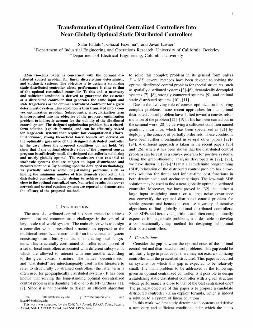
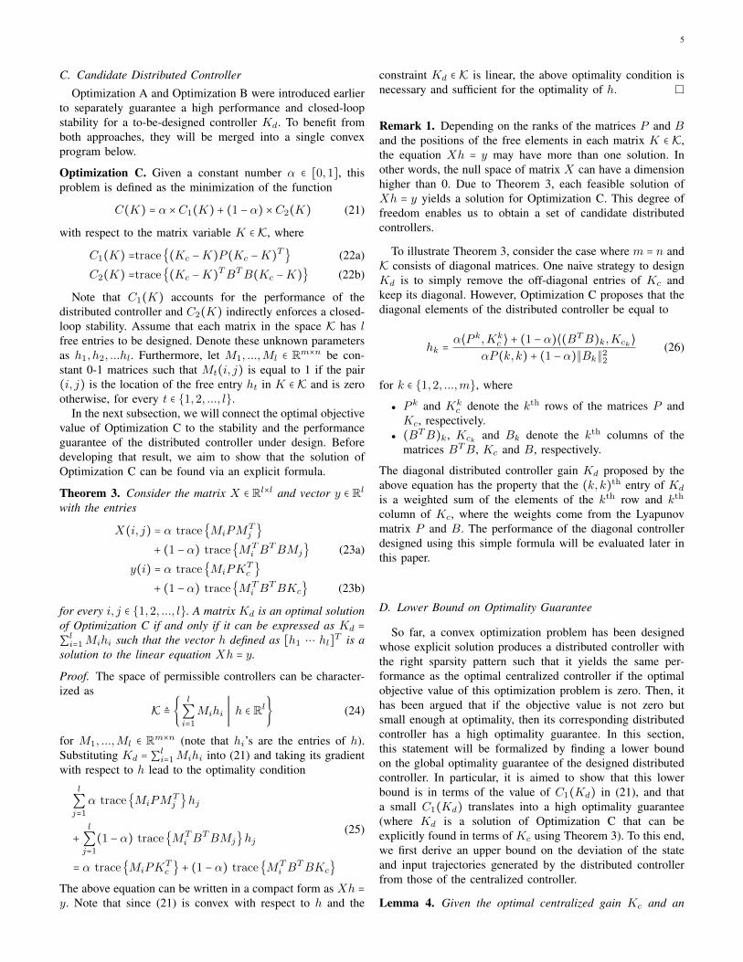
In this part, we study the distributed frequency controlproblem for electrical power systems. The goal is to design adistributed controller that controls the frequency of a systemconsisting of a number of generators and loads that areconnected together via an underlying transmission network.As a case study, we consider the IEEE 39-Bus New EnglandPower System. The Single-line diagram of this system isprovided in Figure 1. The distributed controller constrainedby a user-defined structure is used to optimally adjust themechanical power input to each generator. This pre-determinedcommunication topology specifies which generators exchangetheir rotor angle and frequency measurements with one an-other. To formulate the problem, we consider the widely usedper-unit swing equation

Miθi +Diθi = PMi − PEi (60)

where θi denotes the voltage (or rotor) angle at a generator busi (in rad), PMi is the mechanical power input to the generatorat bus i (in per unit), PEi is the electrical active power injectionat bus i (in per unit), Mi is the inertia coefficient of thegenerator at bus i (in pu-sec2/rad), and Di is the dampingcoefficient of the generator at bus i (in pu-sec/rad) [39]. Theelectrical real power PEi in (60) can be found using thenonlinear AC power flow equation

PEi =n

∑j=1

∣Vi∣∣Vj ∣ [ Gij cos(θi − θj) +Bij sin(θi − θj) ]

(61)where n denotes the number of buses in the system, Vi isthe voltage phasor at bus i, Gij is the line conductance, andBij is the line susceptance. To simplify the formulation, a

Fig. 1: Single-line diagram of IEEE 39-Bus New England Power System.

commonly-used technique is to use the DC power flow equa-tion corresponding to (61) in which all the voltage magnitudesare assumed to be 1 per unit, each branch is modeled as aseries inductor, and the angle differences across the lines areassumed to be relatively small:

PEi =n

∑j=1

Bij(θi − θj) (62)

It is possible to rewrite (62) into the matrix format PE = Lθ,where PE and θ are the vectors of real power injections andvoltage (or rotor) angles at only the generator buses. In thisequation, L denotes the Laplacian matrix and can be found asfollows [40]:

Lii =n

∑j=1,j≠i

BKronij if i = j

Lij = −BKronij if i ≠ j

(63)

where BKron is the susceptance of the Kron reduced admit-tance matrix Y Kron defined as

Y Kronij = Yij −

YikYkj

Ykk(i, j = 1,2, . . . , n and i, j ≠ k) (64)

where k is the index of the non-generator bus to be eliminatedfrom the admittance matrix and n is the number of generatorbuses. Note that the Kron reduction method aims to eliminatethe static buses of the network because the dynamics andinteractions of only the generator buses are of interest [41].

Using θ = [θ1, . . . , θn]T as rotor angle state vector and w =

[w1, . . . ,wn]T as the frequency state vector and substituting

the matrix format of PE into (60), the state space model of theswing equation used for frequency control in power systemscould be written as

[θw] = [

0n×n In−M−1L −M−1D

] [θw] + [

0n×nM−1]PM

y = [θw]

(65)

11

(a) Fully Distributed (b) Localized

(c) Star Topology (G10 in center) (d) Ring

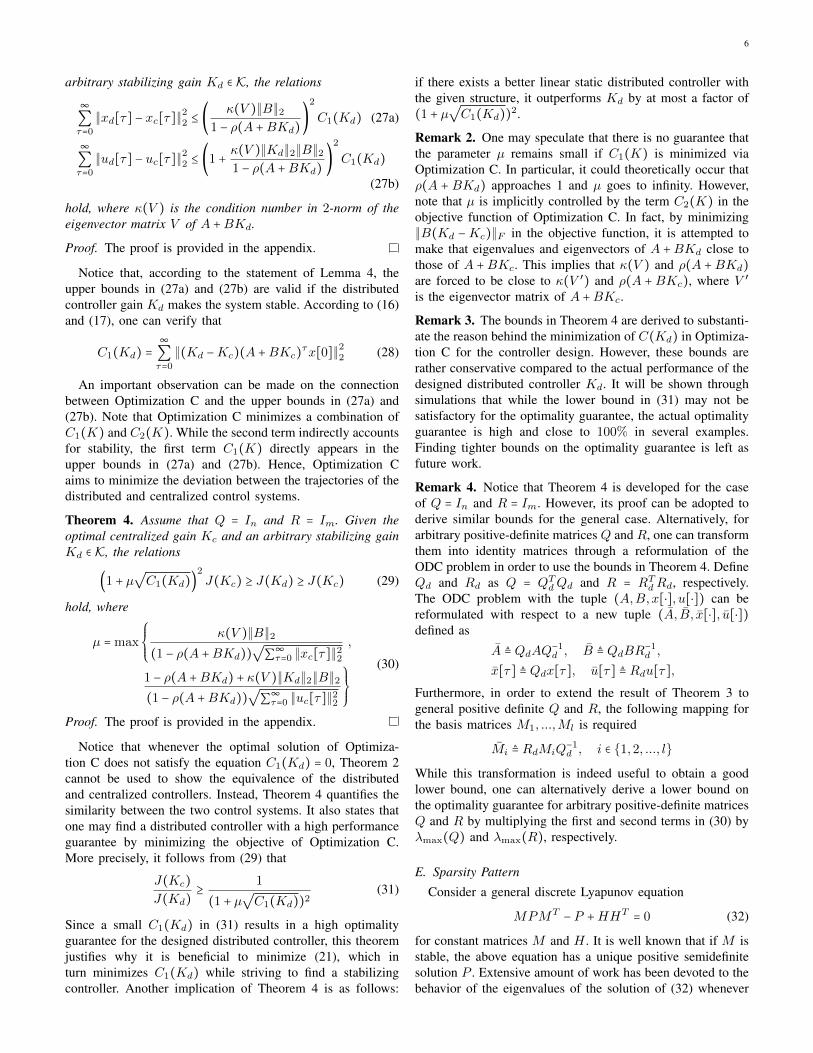
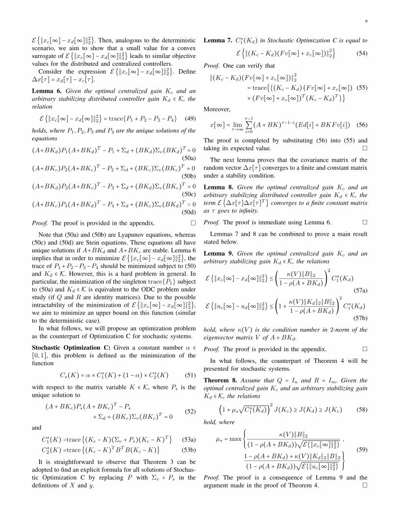
Fig. 2: Communication structures studied in Example 1 for the IEEE 39-Bustest System (borrowed from [31]).

where M = diag(M1, . . . ,Mn) and D = diag(D1, . . . ,Dn).The details of this modeling may be found in [30].

The goal is to first discretize the system with the samplingtime of 0.2 second, and then design a distributed controllerto stabilize the system while achieving a high degree ofoptimality. The 39-bus system has 10 generators, labeled asG1,G2, ...,G10. We consider four different topologies for thestructure of the controller: distributed, localized, star and ring.A visual illustration of these topologies is provided in Figure 2,where each node represents a generator and each line specifieswhat generators are allowed to communicate. We will studyboth deterministic and stochastic cases below, by choosingthe entries of the initial state x(0) uniformly from the interval[0,1].

Deterministic Case: In this experiment, we generate theweighting matrices Q and R in a random fashion as Q = QQT

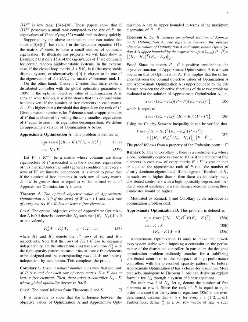
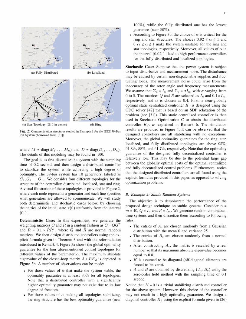
and R = 0.1 × RRT , where Q and R are normal randommatrices. We then design distributed controllers using the ex-plicit formula given in Theorem 3 and with the reformulationintroduced in Remark 4. Figure 3a shows the global optimalityguarantee for the four aforementioned control topologies fordifferent values of the parameter α. The maximum absoluteeigenvalue of the closed-loop matrix A +BKd is depicted inFigure 3b. A number of observations can be made:

● For those values of α that make the system stable, theoptimality guarantee is at least 80% for all topologies.Note that a distributed controller with a significantlyhigher optimality guarantee may not exist due to its lowdegree of freedom.

● For those values of α making all topologies stabilizing,the ring structure has the best optimality guarantee (near

100%), while the fully distributed one has the lowestguarantee (near 80%).

● According to Figure 3b, the choice of α is critical for thering and star structures. The choices 0.92 ≤ α ≤ 1 and0.77 ≤ α ≤ 1 make the system unstable for the ring andstar topologies, respectively. Moreover, all values of α inthe interval [0.02,1] lead to high-performance controllersfor the fully distributed and localized topologies.

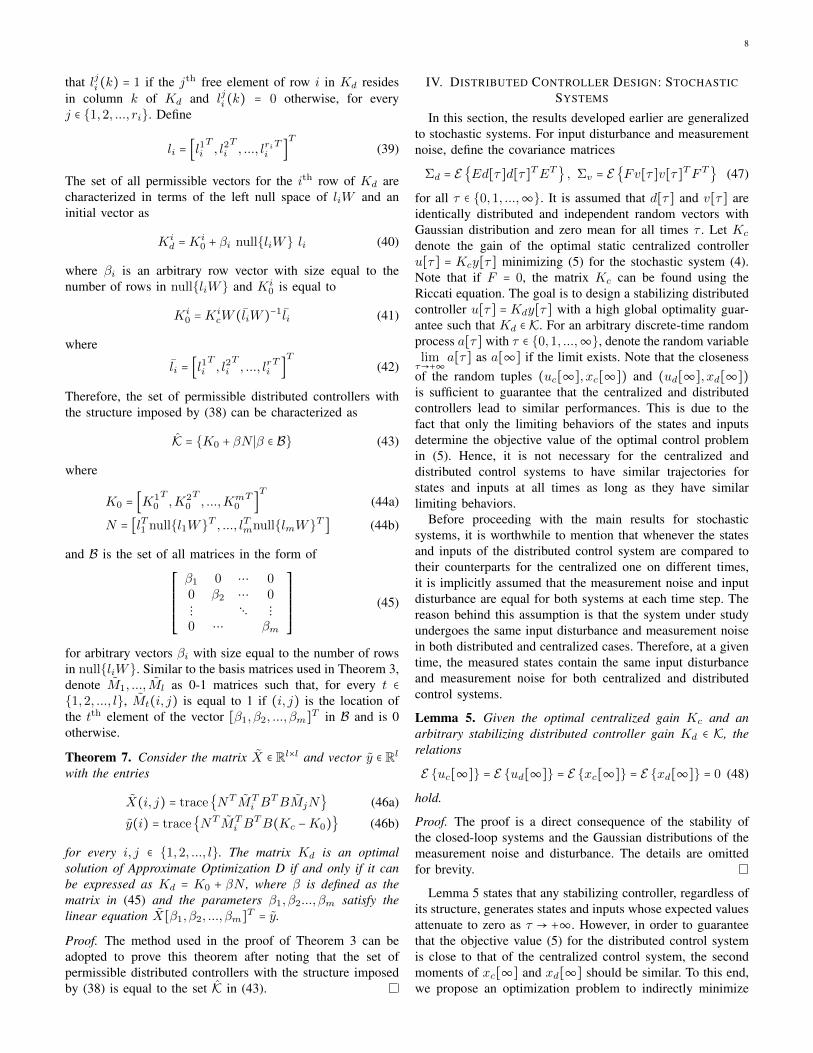
Stochastic Case: Suppose that the power system is subjectto input disturbance and measurement noise. The disturbancemay be caused by certain non-dispatchable supplies and fluc-tuating loads. The measurement noise could arise from theinaccuracy of the rotor angle and frequency measurements.We assume that Σd = In and Σv = σIn, with σ varying from0 to 5. The matrices Q and R are selected as In and 0.1×Im,respectively, and α is chosen as 0.4. First, a near-globallyoptimal static centralized controller Kc is designed using theODC solver [42] that is based on an SDP relaxation of theproblem (see [31]). This static centralized controller is thenused in Stochastic Optimization C to obtain the distributedcontroller Kd, as explained in Remark 6. The simulationresults are provided in Figure 4. It can be observed that thedesigned controllers are all stabilizing with no exceptions.Moreover, the global optimality guarantees for the ring, star,localized, and fully distributed topologies are above 95%,91.8%, 88%, and 61.7%, respectively. Note that the optimalityguarantee of the designed fully decentralized controller isrelatively low. This may be due to the potential large gapbetween the globally optimal costs of the optimal centralizedand fully decentralized control problems. Furthermore, noticethat the designed distributed controllers are all found using theexplicit formulas provided in this paper, as opposed to solvingoptimization problems.

B. Example 2: Stable Random Systems

The objective is to demonstrate the performance of theproposed design technique on stable systems. Consider n =

m = 40, Q = In and R = Im. We generate random continuous-time systems and then discretize them according to followingrules:

● The entries of Ac are chosen randomly from a Gaussiandistribution with the mean 0 and variance 25.

● The entries of Bc are chosen randomly from a normaldistribution.

● After constructing Ac, the matrix is rescaled by a realnumber so that its maximum absolute eigenvalue becomesequal to 0.8.

● K is assumed to be diagonal (off-diagonal elements areforced to be zero).

● A and B are obtained by discretizing (Ac,Bc) using thezero-order hold method with the sampling time of 0.1second.

Notice that K = 0 is a trivial stabilizing distributed controllerfor the above system. However, this choice of the controllermay not result in a high optimality guarantee. We design adiagonal controller Kd using the explicit formula given in (26)

12

α

0 0.2 0.4 0.6 0.8 1

Glo

ba

l O

ptim

alit

y G

ua

ran

tee

0

20

40

60

80

100

Fully DecentralizedLocalizedStarRing

(a) Optimality Guaranteeα

0 0.2 0.4 0.6 0.8 1

Ma

xim

um

Ab

so

lute

Eig

en

va

lue

0.8

0.9

1

1.1

1.2

1.3Fully DecentralizedLocalizedStarRing

(b) Maximum Absolute Eigenvalues

Fig. 3: Global optimality guarantee and maximum absolute eigenvalue of A +BKd for four different topologies and different values of α (deterministiccase).

σ

0 1 2 3 4 5

Optim

alit

y G

uara

nte

e

60

70

80

90

100

Fully DecentralizedLocalizedStarRing

(a) Optimality Guaranteeσ

0 1 2 3 4 5

Ma

xim

um

Ab

so

lute

Eig

en

va

lue

0.94

0.95

0.96

0.97

0.98

0.99

1

Fully DecentralizedLocalizedStarRing

(b) Maximum Absolute Eigenvalues

Fig. 4: Global optimality guarantee and maximum absolute eigenvalue of A + BKd for four different topologies and different values of σ, under theassumptions Σd = In and Σv = σIn (stochastic case).

trials0 20 40 60 80 100

Glo

ba

l O

ptim

alit

y G

ua

ran

tee

20

30

40

50

60

70

80

90

100

Designed Kd

Kd=0

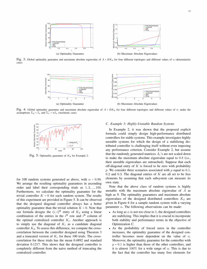
Fig. 5: Optimality guarantee of Kd for Example 2.

for 100 random systems generated as above, with α = 0.98.We arrange the resulting optimality guarantees in ascendingorder and label their corresponding trials as 1,2, ...,100.Furthermore, we calculate the optimality guarantee for thetrivial controller K = 0 for each random system. The resultsof this experiment are provided in Figure 5. It can be observedthat the designed diagonal controller always has a betteroptimality guarantee than the trivial solution K = 0. Note thatour formula designs the (i, i)th entry of Kd using a linearcombination of the entries in the ith row and ith column ofthe optimal centralized controller Kc. Another approach isto simply use the diagonal of Kc as a candidate diagonalcontroller Kd. To assess this difference, we compute the cross-correlation between the controller designed using Theorem 3and a truncated version of Kc for these 100 trials. The cross-correlation for these trials has the mean 0.4892 and standarddeviation 0.1217. This shows that the designed controller iscompletely different from the naive method of truncating thecentralized controller.

C. Example 3: Highly-Unstable Random Systems

In Example 2, it was shown that the proposed explicitformula could simply design high-performance distributedcontrollers for stable systems. This example investigates highlyunstable systems for which the design of a stabilizing dis-tributed controller is challenging itself without even imposingany performance criterion. Consider Example 2, but assumethat the randomly generated matrices Ac’s are not scaled downto make the maximum absolute eigenvalue equal to 0.8 (i.e.,their unstable eigenvalues are untouched). Suppose that eachoff-diagonal entry of K is forced to be zero with probabilityp. We consider three scenarios associated with p equal to 0.1,0.2 and 0.3. The diagonal entries of K are all set to be freeelements by assuming that each subsystem can measure itsown state.

Note that the above class of random systems is highlyunstable with the maximum absolute eigenvalue of A ashigh as 9. The optimality guarantees and maximum absoluteeigenvalues of the designed distributed controllers Kd aregiven in Figure 6 for a sample random system with a varyingparameter α. The following observations can be made:

● As long as α is not too close to 1, the designed controllersare stabilizing. This implies that it is crucial to incorporateboth stability and performance terms in the objective ofOptimization C.

● As the probability of forced zeros in the controllerincreases, the optimality guarantee of the designed con-troller becomes more dependent on the value of α.Moreover, the optimality guarantee for the controller withp = 0.1 is higher than those of the other controllers, andit is almost 100% for a wide range of α. This is due tothe fact that the controller has many free elements for

13

α

0 0.2 0.4 0.6 0.8 1

Glo

ba

l O

ptim

alit

y G

ua

ran

tee

0

20

40

60

80

100p = 0.1p = 0.2p = 0.3

(a) Optimality Degreeα

0 0.2 0.4 0.6 0.8 1Ma

xim

um

Ab

so

lute

Eig

en

va

lue

0

2

4

6

8

10p = 0.1p = 0.2p = 0.3

(b) Maximum Absolute Eigenvalues

Fig. 6: Optimality guarantee and maximum absolute eigenvalue of A +BKd for a highly-unstable random system in Example 3.

trials0 20 40 60 80 100

Glo

ba

l O

ptim

alit

y G

ua

ran

tee

0

20

40

60

80

100p=0.1p=0.2p=0.3

(a) Optimality Degreetrials

0 20 40 60 80 100

Ma

x A

bso

lute

Eig

en

va

lue

0.4

0.6

0.8

1

1.2

1.4

1.6p=0.1p=0.2p=0.3

Ma

xim

um

Ab

so

lute

Eig

en

va

lue

(b) Maximum Absolute Eigenvalues

Fig. 7: Optimality guarantee and maximum absolute eigenvalue of A +BKd.

design.

Now, consider 100 random systems generated according to theaforementioned rules and set α = 0.98. We design distributedcontrollers for the three scenarios of p equal to 0.1, 0.2 and0.3. We arrange the obtained maximum absolute eigenvaluesin ascending order and subsequently label their correspondingtrials as 1,2, ...,100. Figure 7 shows the optimality guar-antees and maximum absolute eigenvalues of the designeddistributed controllers. For p = 0.1, the proposed methodalways yields stabilizing controllers with optimality guaranteesnear to 100%. For p = 0.2, 99 control systems are stable withoptimality guarantees near to 100%. For p = 0.3, 54 controlsystems are stable with high optimality guarantees. Note thatthe designed controllers are different from truncated versionsof Kc (by simply discarding 10%-30% entries of Kc). Moreprecisely, the cross-correlation between the controller designedusing Theorem 3 and a truncated version of Kc for the above100 trials with p = 0.1 has the mean 0.6245 and standarddeviation 0.0677.

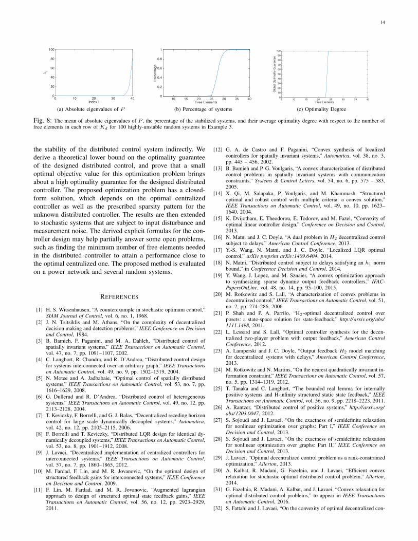
As mentioned earlier, the eigenvalues of P in the Lyapunovequation (14) may decay rapidly. To support this statement,we compute the eigenvalues of P for previously generated100 random unstable systems. Subsequently, we arrange theabsolute eigenvalues of P for each system in ascending orderand label them as λ1, λ2, ..., λ40. For every i ∈ {1,2, ...,40},the mean of λi for these 100 independent random systemsis drawn in Figure 8a (the variance is very low). It can beobserved that only 15% of the eigenvalues are dominant andP can be well approximated by a low-rank matrix. Due toCorollary 1, in order to ensure a high optimality guarantee,each row of Kd should have at least 6 free elements. However,as discussed earlier, more free elements may be required tomake the system stable via Approximate Optimization D. Tostudy the minimum number of free elements needed to achieve

a closed-loop stability and a high optimality guarantee, wefind distributed controllers using Approximate Optimization Dfor different numbers of free elements at each row of Kd. Inall of these random systems, P is approximated by a rank-6 matrix P . For each sparsity level, we then calculate thepercentage of closed-loop systems that become stable usingApproximate Optimization D. Moreover, their average globaloptimality guarantee using the designed Kd is also obtained.The results are provided in Figures 8b and 8c. The number ofstable closed-loop systems increases quickly as the numberof free elements in each row of the distributed controllergain exceeds 25. As mentioned earlier, there could be a non-trivial gap between the minimum number of free elementssatisfying the performance criterion and the minimum numberof free elements required to make the closed-loop systemstable. Furthermore, it can be observed in Figure 8c that thedesigned distributed controller has an optimality guaranteeclose to 100% for all stable closed-loop systems. This optimal-ity guarantee is ensured via constraint (38c) in ApproximateOptimization D.

VI. CONCLUSIONS

This paper studies the optimal distributed control prob-lem for linear discrete-time systems. The goal is to designa stabilizing static distributed controller with a pre-definedstructure, whose performance is close to that of the best (static)centralized controller. To this end, we derive a necessaryand sufficient condition under which there exists a distributedcontroller that produces the same input and state trajectoriesas the optimal centralized controller for a given deterministicsystem. We then convert this condition into a convex opti-mization problem. We also add a regularization term into theobjective of the proposed optimization problem to account for

14

index i

0 10 20 30 40

λi

0

20

40

60

80

100

(a) Absolute eigenvalues of PFree Elements

10 15 20 25 30 35 40

Perc

enta

ge

0

0.2

0.4

0.6

0.8

1

(b) Percentage of systemsFree Elements

5 10 15 20 25 30 35 40

Glo

bal O

ptim

alit

y G

uara

nte

e

0

10

20

30

40

50

60

70

80

90

100

(c) Optimality Degree

Fig. 8: The mean of absolute eigenvalues of P , the percentage of the stabilized systems, and their average optimality degree with respect to the number offree elements in each row of Kd for 100 highly-unstable random systems in Example 3.

the stability of the distributed control system indirectly. Wederive a theoretical lower bound on the optimality guaranteeof the designed distributed control, and prove that a smalloptimal objective value for this optimization problem bringsabout a high optimality guarantee for the designed distributedcontroller. The proposed optimization problem has a closed-form solution, which depends on the optimal centralizedcontroller as well as the prescribed sparsity pattern for theunknown distributed controller. The results are then extendedto stochastic systems that are subject to input disturbance andmeasurement noise. The derived explicit formulas for the con-troller design may help partially answer some open problems,such as finding the minimum number of free elements neededin the distributed controller to attain a performance close tothe optimal centralized one. The proposed method is evaluatedon a power network and several random systems.

REFERENCES

[1] H. S. Witsenhausen, “A counterexample in stochastic optimum control,”SIAM Journal of Control, vol. 6, no. 1, 1968.

[2] J. N. Tsitsiklis and M. Athans, “On the complexity of decentralizeddecision making and detection problems,” IEEE Conference on Decisionand Control, 1984.

[3] B. Bamieh, F. Paganini, and M. A. Dahleh, “Distributed control ofspatially invariant systems,” IEEE Transactions on Automatic Control,vol. 47, no. 7, pp. 1091–1107, 2002.

[4] C. Langbort, R. Chandra, and R. D’Andrea, “Distributed control designfor systems interconnected over an arbitrary graph,” IEEE Transactionson Automatic Control, vol. 49, no. 9, pp. 1502–1519, 2004.

[5] N. Motee and A. Jadbabaie, “Optimal control of spatially distributedsystems,” IEEE Transactions on Automatic Control, vol. 53, no. 7, pp.1616–1629, 2008.

[6] G. Dullerud and R. D’Andrea, “Distributed control of heterogeneoussystems,” IEEE Transactions on Automatic Control, vol. 49, no. 12, pp.2113–2128, 2004.

[7] T. Keviczky, F. Borrelli, and G. J. Balas, “Decentralized receding horizoncontrol for large scale dynamically decoupled systems,” Automatica,vol. 42, no. 12, pp. 2105–2115, 2006.

[8] F. Borrelli and T. Keviczky, “Distributed LQR design for identical dy-namically decoupled systems,” IEEE Transactions on Automatic Control,vol. 53, no. 8, pp. 1901–1912, 2008.

[9] J. Lavaei, “Decentralized implementation of centralized controllers forinterconnected systems,” IEEE Transactions on Automatic Control,vol. 57, no. 7, pp. 1860–1865, 2012.

[10] M. Fardad, F. Lin, and M. R. Jovanovic, “On the optimal design ofstructured feedback gains for interconnected systems,” IEEE Conferenceon Decision and Control, 2009.

[11] F. Lin, M. Fardad, and M. R. Jovanovic, “Augmented lagrangianapproach to design of structured optimal state feedback gains,” IEEETransactions on Automatic Control, vol. 56, no. 12, pp. 2923–2929,2011.

[12] G. A. de Castro and F. Paganini, “Convex synthesis of localizedcontrollers for spatially invariant systems,” Automatica, vol. 38, no. 3,pp. 445 – 456, 2002.

[13] B. Bamieh and P. G. Voulgaris, “A convex characterization of distributedcontrol problems in spatially invariant systems with communicationconstraints,” Systems & Control Letters, vol. 54, no. 6, pp. 575 – 583,2005.

[14] X. Qi, M. Salapaka, P. Voulgaris, and M. Khammash, “Structuredoptimal and robust control with multiple criteria: a convex solution,”IEEE Transactions on Automatic Control, vol. 49, no. 10, pp. 1623–1640, 2004.

[15] K. Dvijotham, E. Theodorou, E. Todorov, and M. Fazel, “Convexity ofoptimal linear controller design,” Conference on Decision and Control,2013.

[16] N. Matni and J. C. Doyle, “A dual problem in H2 decentralized controlsubject to delays,” American Control Conference, 2013.

[17] Y.-S. Wang, N. Matni, and J. C. Doyle, “Localized LQR optimalcontrol,” arXiv preprint arXiv:1409.6404, 2014.

[18] N. Matni, “Distributed control subject to delays satisfying an h1 normbound,” in Conference Decision and Control, 2014.

[19] Y. Wang, J. Lopez, and M. Sznaier, “A convex optimization approachto synthesizing sparse dynamic output feedback controllers,” IFAC-PapersOnLine, vol. 48, no. 14, pp. 95–100, 2015.

[20] M. Rotkowitz and S. Lall, “A characterization of convex problems indecentralized control,” IEEE Transactions on Automatic Control, vol. 51,no. 2, pp. 274–286, 2006.

[21] P. Shah and P. A. Parrilo, “H2-optimal decentralized control overposets: a state-space solution for state-feedback,” http://arxiv.org/abs/1111.1498, 2011.

[22] L. Lessard and S. Lall, “Optimal controller synthesis for the decen-tralized two-player problem with output feedback,” American ControlConference, 2012.

[23] A. Lamperski and J. C. Doyle, “Output feedback H2 model matchingfor decentralized systems with delays,” American Control Conference,2013.

[24] M. Rotkowitz and N. Martins, “On the nearest quadratically invariant in-formation constraint,” IEEE Transactions on Automatic Control, vol. 57,no. 5, pp. 1314–1319, 2012.

[25] T. Tanaka and C. Langbort, “The bounded real lemma for internallypositive systems and H-infinity structured static state feedback,” IEEETransactions on Automatic Control, vol. 56, no. 9, pp. 2218–2223, 2011.

[26] A. Rantzer, “Distributed control of positive systems,” http://arxiv.org/abs/1203.0047, 2012.

[27] S. Sojoudi and J. Lavaei, “On the exactness of semidefinite relaxationfor nonlinear optimization over graphs: Part I,” IEEE Conference onDecision and Control, 2013.

[28] S. Sojoudi and J. Lavaei, “On the exactness of semidefinite relaxationfor nonlinear optimization over graphs: Part II,” IEEE Conference onDecision and Control, 2013.

[29] J. Lavaei, “Optimal decentralized control problem as a rank-constrainedoptimization,” Allerton, 2013.

[30] A. Kalbat, R. Madani, G. Fazelnia, and J. Lavaei, “Efficient convexrelaxation for stochastic optimal distributed control problem,” Allerton,2014.

[31] G. Fazelnia, R. Madani, A. Kalbat, and J. Lavaei, “Convex relaxation foroptimal distributed control problems,” to appear in IEEE Transactionson Automatic Control, 2016.

[32] S. Fattahi and J. Lavaei, “On the convexity of optimal decentralized con-

15

trol problem and sparsity path,” http://www.ieor.berkeley.edu/∼lavaei/SODC 2016.pdf , 2016.

[33] G. Dullerud and F. Paganini, Course in Robust Control Theory.Springer-Verlag New York, 2000.

[34] P. Benner, J. Li, and T. Penzl, “Numerical solution of largescale lya-punov equations, riccati equations, and linearquadratic optimal controlproblems,” Numerical Linear Algebra with Applications, vol. 15, no. 9,pp. 755–777, 2008.

[35] L. Grubisic and D. Kressner, “On the eigenvalue decay of solutions tooperator lyapunov equations,” Systems and control letters, vol. 73, pp.42–47, 2014.

[36] J. Baker, M. Embree, and J. Sabino, “Fast singular value decay forlyapunov solutions with nonnormal coefficients,” SIAM Journal onMatrix Analysis and Applications, vol. 36, no. 2, pp. 656–668, 2015.

[37] L. Grasedyck, W. Hackbusch, and B. N. Khoromskij, “Solution of largescale algebraic matrix riccati equations by use of hierarchical matrices,”Computing, vol. 70, no. 2, pp. 121–165, 2003.

[38] T. Penzl, “Eigenvalue decay bounds for solutions of lyapunov equations:the symmetric case,” Systems and Control Letters, vol. 40, no. 2, pp.139–144, 2000.

[39] M. A. Pai, Energy Function Analysis for Power System Stability. KluwerAcademic Publishers, Boston, 1989.

[40] F. Dorfler and F. Bullo, “Novel insights into lossless AC and DC powerflow,” IEEE Power and Energy Society General Meeting, 2013.

[41] A. R. Bergen and V. Vittal, Power Systems Analysis. Prentice Hall,1999, vol. 2.

[42] G. Fazelnia and J. Lavaei, “ODC Solver,” http://www.ee.columbia.edu/∼lavaei/Software.html, 2014.

APPENDIX

Proof of Lemma 1: Note thatxd[τ] = (A +BKd)

τx[0]

xc[τ] = (A +BKc)τx[0]

(66)

To prove the necessity part, suppose that xd[τ] = xc[τ] andxd[τ + 1] = xc[τ + 1]. One can write

0 = (A +BKd)τ+1x[0] − (A +BKc)

τ+1x[0]

= (A +BKd)(A +BKc)τx[0] − (A +BKc)

τ+1x[0]

= B(Kc −Kd)(A +BKc)τx[0]

To prove the sufficiency part, we use a mathematical induction.The validity of the base case can be easily verified. Assumethat xd[k] = xc[k] for τ = k, and consider the case τ = k + 1.It follows from the equality BKc(A+BKc)

τx[0] = BKd(A+BKd)

τx[0] of the induction step that

(A +BKc)k+1x[0] = A(A +BKd)

kx[0]

+BKd(A +BKd)kx[0]

= (A +BKd)k+1x[0]

This completes the proof. ◻

Proof of Lemma 2: First, we aim to show that (9) im-plies (10). To this end, assume that the equation (9) is satisfied.Since xc[0] = xd[0] = x[0], the relation xc[τ] = xd[τ] holdsfor every nonnegative integer τ (note that the system (1)generates identical state signals under two identical inputsignals uc[τ] and ud[τ] ). Now, one can write

uc[τ] =Kcxc[τ] =Kc(A +BKc)τx[0] (67a)

ud[τ] =Kdxd[τ] =Kd(A +BKd)τx[0] (67b)

On the other hand, the relation xc[τ] = xd[τ] can be ex-pressed as

(A +BKc)τx[0] = (A +BKd)

τx[0] (68)

Combining (67) and (68) leads to (10).To prove that (10) implies (9), suppose that the equation (10)

is satisfied. By pre-multiply the left side of (10) with B, itfollows from Lemma 1 that xc[τ] = xd[τ]. Therefore,

uc[τ] − ud[τ] =Kcxc[τ] −Kdxd[τ]

=Kcxc[τ] −Kdxc[τ]

= (Kc −Kd)(A +BKc)τx[0]

= 0

(69)

This yields the equation (9), and completes the proof. ◻

Proof of Lemma 4: First, we prove the inequality (27a). Itis straightforward to verify that

∆x[τ + 1] = B(Kd −Kc)xc[τ] + (A +BKd)∆x[τ] (70)

Consider the eigen-decomposition of A + BKd as V −1DV .Define ∆x[τ] = V∆x[τ]. Multiplying both sides of (70) byV yields that

∆x[τ + 1] = V B(Kd −Kc)xc[τ] +D∆x[τ] (71)

Taking the 2-norm from both sides of (71) leads to

∥∆x[τ + 1]∥2 ≤∥V B(Kd −Kc)xc[τ]∥2

+ ∥D∥2 × ∥∆x[τ]∥2

≤∥V B(Kd −Kc)xc[τ]∥2

+ ρ(A +BKd) × ∥∆x[τ]∥2

(72)

(note that ∥D∆x[τ]∥2 ≤ ∥D∥2∥∆x[τ]∥2 and ∥D∥2 ≤ ρ(A +

BKd)). It can be concluded from (72) that

(∥∆x[τ + 1]∥2 − ρ(A +BKd) × ∥∆x[τ]∥2)2

≤ ∥V B(Kd −Kc)xc[τ]∥22 (73)

or equivalently

∥∆x[τ + 1]∥22 + ρ(A +BKd)

2∥∆x[τ]∥2

2

− 2ρ(A +BKd)∥∆x[τ + 1]∥2∥∆x[τ]∥2

≤ ∥V B(Kd −Kc)xc[τ]∥22 (74)

Summing up both sides of (74) over all values of τ gives riseto the inequality

∞

∑τ=0

∥∆x[τ + 1]∥22 + ρ(A +BKd)

2∞

∑τ=0

∥∆x[τ]∥22

− 2ρ(A +BKd)∞

∑τ=0

∥∆x[τ + 1]∥2∥∆x[τ]∥2

≤∞

∑τ=0

∥V B(Kd −Kc)(xc[τ])∥22 (75)

Using the Cauchy-Schwarz inequality, one can write

∞

∑τ=0

∥∆x[τ + 1]∥22 + ρ(A +BKd)

2∞

∑τ=0

∥∆x[τ]∥22

− 2ρ(A +BKd)

¿ÁÁÀ(

∞

∑τ=0

∥∆x[τ + 1]∥22)(

∞

∑τ=0

∥∆x[τ]∥22)

≤∞

∑τ=0

∥V B(Kd −Kc)(xc[τ])∥22 (76)

16

Note that ∑∞τ=0 ∥∆x[τ + 1]∥22 = ∑

∞τ=0 ∥∆x[τ]∥2

2. Hence, it canbe inferred from (76) and (28) that

∞

∑τ=0

∥∆x[τ]∥22 ≤ (

∥V ∥2∥B∥2

1 − ρ(A +BKd))

2

C1(Kd) (77)

Since ∆x[τ] = V −1∆x[τ], one can write∞

∑τ=0

∥∆x[τ]∥22 ≤ ∥V −1

∥22

∞

∑τ=0

∥∆x[τ]∥22

≤ (∥V −1∥2∥V ∥2∥B∥2

1 − ρ(A +BKd))

2

C1(Kd)

(78)

This proves the inequality (27a). The above argument can beadopted to prove (27b) after noting that

∆u[τ] = (Kd −Kc)xc[τ] +Kd∆x[τ] (79)

where ∆u[τ] = ud[τ] − uc[τ]. ◻

Proof of Theorem 4: According to Lemma 4, one can write

∞

∑τ=0

∥xd[τ]∥22+

∞

∑τ=0

∥xc[τ]∥22 ≤ (

κ(V )∥B∥2

1 − ρ(A +BKd))

2

C1(Kd)

+ 2∞

∑τ=0

∥xc[τ]∥2∥xd[τ]∥2 (80)

Dividing both sides of (80) by ∑∞τ=0 ∥xc[τ]∥22 and using the

Cauchy-Schwarz inequality for ∑∞τ=0 ∥xc[τ]∥2∥xd[τ]∥2 yieldthat

∑∞τ=0 ∥xd[τ]∥

22

∑∞τ=0 ∥xc[τ]∥2

2

≤⎛

⎝1 +

κ(V )∥B∥2

(1 − ρ(A +BKd))√∑∞τ=0 ∥xc[τ]∥2

2

√C1(Kd)

⎞

⎠

2

(81)Likewise,

∑∞τ=0 ∥ud[τ]∥

22

∑∞τ=0 ∥uc[τ]∥2

2

≤⎛

⎝1 +

1 − ρ(A +BKd) + κ(V )∥Kd∥2∥B∥2

(1 − ρ(A +BKd))√∑∞τ=0 ∥uc[τ]∥2

2

√C1(Kd)

⎞

⎠

2

(82)Combining (81) and (82) leads to

J(Kd)

J(Kc)=∑∞τ=0 ∥xd[τ]∥

22 +∑

∞τ=0 ∥ud[τ]∥

22

∑∞τ=0 ∥xc[τ]∥2

2 +∑∞τ=0 ∥uc[τ]∥2

2

≤ (1 + µ√C1(Kd))

2

(83)

This completes the proof. ◻

Proof of Lemma 6: It is straightforward to verify that

E {∥xc[∞] − xd[∞]∥22} = trace{E {xd[∞]xd[∞]

T }}

+ trace{E {xc[∞]xc[∞]T }}

− trace{E {xd[∞]xc[∞]T }}

− trace{E {xc[∞]xd[∞]T }}

(84)

On the other hand, since d[⋅] and v[⋅] are independentand identically distributed random vectors, the equation

E {d[τ1]d[τ2]T } = E {v[τ1]v[τ2]

T } = 0 holds for ev-ery two different indices τ1 and τ2. In addition, we haveE {v[τ1]d[τ2]

T } = E {d[τ1]v[τ2]T } = 0, for all nonnative

integers τ1 and τ2. It follows from these relations and theequations (84) and (56) that

E {xd[τ]xd[τ]T } = P1, E {xc[τ]xc[τ]

T } = P2,

E {xd[τ]xc[τ]T } = P3, E {xc[τ]xd[τ]

T } = P4,(85)

where P1, P2, P3 and P4 satisfy (50). Moreover, note that(50a) and (50b) are Lyapunov equations, whereas (50c) and(50d) are Stein equations. These equations all have uniquesolutions since A + BKd and A + BKc are stable. Thiscompletes the proof. ◻

Proof of Lemma 9: The proof is similar to that of Lemma 4.First, we prove the inequality (57a). It is straightforward toverify that

∆x[τ +1] = B(Kd −Kc)(Fv[τ]+xc[τ])+ (A+BKd)∆x[τ](86)

Using the eigen-decomposition of A + BKd as V −1DV andpursuing the method developed in the proof of Lemma 4, onecan write

E {(∥∆x[τ + 1]∥2 − ρ(A +BKd) × ∥∆x[τ]∥2)2}

≤ E {∥V B(Kd −Kc)(Fv[τ] + xc[τ])∥22} (87)

where ∆x[τ] = V∆x[τ]. It follows from the Cauchy-Schwarzinequality and (87) that

E {∥∆x[τ + 1]∥22} + ρ(A +BKd)

2E {∥∆x[τ]∥2

2}

− 2ρ(A +BKd)

√

E {∥∆x[τ + 1]∥22}E {∥∆x[τ]∥

22}

≤ E {∥V B(Kd −Kc)(Fv[τ] + xc[τ])∥22} (88)

According to Lemma 8, E {∆x[τ]∆x[τ]T } (and hence,E {∆x[τ]∆x[τ]∗}) converges to a constant matrix as τ ap-proaches infinity. This implies that E {∥∆x[τ + 1]∥2

2} andE {∥∆x[τ]∥2

2} converge to the same number. Taking the limitsfrom both sides of (88) and interchanging the limit operatorwith the expected value operator result in

E {∥∆x[∞]∥22} ≤ (

∥V ∥2∥B∥2

1 − ρ(A +BKd))

2

Cs1(Kd) (89)

Substituting ∆x[∞] = V −1∆x[∞] into the above inequalityleads to

E {∥∆x[∞]∥22} ≤ ∥V −1

∥22 × E {∥∆x[∞]∥

22}

≤ (∥V −1∥2∥V ∥2∥B∥2

1 − ρ(A +BKd))

2

Cs1(Kd)(90)

The inequality (57b) can be proved similarly. ◻