logic-based outer approximation for globally optimal...
TRANSCRIPT

1
Logic-Based Outer Approximation for Globally Optimal Synthesis of Process Networks
Maria Lorena Bergamini#, Pio Aguirre# and Ignacio Grossmann+*
# INGAR – Instituto de Desarrollo y Diseño, Avellaneda 3657, (S3002GJC), Santa Fe, Argentina + Department of Chemical Engineering, Carnegie Mellon University, Pittsburgh, PA 15213, USA
Abstract Process network problems can be formulated as Generalized Disjunctive Programs where a logic-based representation is used to deal with the discrete and continuous decisions. A new deterministic algorithm for the global optimization of process networks is presented in this work. The proposed algorithm, which does not rely on spatial branch-and-bound, is based on the Logic-Based Outer Approximation that exploits the special structure of flowsheet synthesis models. The method is capable of considering nonconvexities, while guaranteeing globality in the solution of an optimal synthesis of process network problem. This is accomplished by solving iteratively reduced NLP subproblems to global optimality and MILP master problems, which are valid outer approximations of the original problem. Piecewise linear under and overestimators for bilinear and concave terms have been constructed with the property of having zero gap in a finite set of points. The global optimization of the reduced NLP may be performed either with a suitable global solver or using the inner optimization strategy that is proposed in this work. Theoretical properties are discussed as well as several alternatives for implementing the proposed algorithm. Several examples were successfully solved with this algorithm. Results show that only few iterations are required to solve them to global optimality.
1. Introduction.
The synthesis of process networks can be formulated as Generalized Disjunctive Programming (GDP) problems. GDP is an alternative to Mixed Integer Non-linear Programming (MINLP) for modeling problems where both continuous and discrete decisions are involved. GDP allows the combination of algebraic and logic equations to represent a synthesis problem in a more natural way.
GDP problems can be solved as MINLP problems by replacing each disjunction with its big-M or its convex hull reformulation (Lee and Grossmann, 2000). Major methods for MINLP problems include Branch-and-Cut, which is a generalization of the linear case (Stubbs and Mehrotra, 1999) Generalized Benders Decomposition (GBD) (Geoffrion, 1972), Outer Approximation (OA) (Duran and Grossmann, 1986, Fletcher and Leyffer, 1994) and Extended Cutting Plane (ECP) method (Westerlund and
* To whom all the correspondence should be addressed

2
Petterson, 1995). GBD and OA are iterative methods that solve a sequence of alternate NLP subproblems with all the discrete variables fixed, and MILP master problems that perform the optimization in the discrete space. The ECP method relies on successive linearizations to build MILP approximation problems.
There are also specific algorithms that exploit the disjunctive structure of the model. In the solution method by Hooker and Osorio (1997) for linear problems, a search tree is created by branching on the logic expressions. A continuous relaxation of the problem is solved at each node of the tree
Lee and Grossmann (2000) presented an optimization algorithm for solving general nonlinear GDP problems. This algorithm consists of a branch-and-bound search that branches on terms of the disjunctions and considers the convex hull relaxation of the remaining disjunctions. Türkay and Grossmann (1996) proposed a Logic-Based Outer Approximation algorithm that solves nonlinear GDP problems for process networks involving two terms in the disjunction. Since the NLP subproblem only involves the active terms of the disjunctions, this algorithm overcomes difficulties that arise in the synthesis of process network problems, such as singularities that are due to zero flows. This algorithm has been implemented in LOGMIP, a computer code developed by Vecchietti and Grossmann (1999).
All the methods mentioned above assume convexity to guarantee convergence to a global solution. Therefore, when applied to nonconvex problems, these algorithms may cut off the global optimum.
Viswanathan and Grossmann (1990) proposed a heuristic modification to the OA algorithm for MINLP in order to reduce the likelihood of cutting-off part of the feasible region. They introduced slacks in the linearization of nonconvex constraints, an included them in an augmented penalty function. The search is stopped when there is no improvement in the NLP subproblems.
Rigorous global optimization methods for addressing nonconvexities in NLP problems have been developed when special structures are assumed in the continuous terms (Quesada and Grossmann, 1995; Ryoo and Sahinidis, 1995; Horst and Tuy, 1996; Viswanathan and Floudas, 1996; Zamora and Grossmann, 1999; Floudas, 2000). Tawarmalani and Sahinidis (2002) have developed the Branch-And-Reduce-Optimization-Navigator (BARON), a software for general purpose global optimization that implements a spatial branch-and-bound method combined with reduction techniques for the variables bounds. For nonconvex MINLP problems Smith and Pantelides (1999), Adjman et al (2000), Tawarmalani and Sahinidis (2000) and Kesavan and Barton (2000) have proposed global optimization algorithms based on spatial branch-and-bound search. Lee and Grossmann (2001) proposed a two-level branching scheme for solving nonconvex GDP problems to global optimality and specialized the algorithm to GDP problem with bilinear equality constraints (2002).
Spatial branch-and-bound methods can be computationally expensive, since the tree may not be finite (except for ε-convergence). For the case of process networks there is the added complication that the NLP subproblems are usually difficult and expensive to solve. Thus, there is a strong motivation for developing a decomposition algorithm for this class of problems that does not rely on spatial branch-and-bound.

3
An outer-approximation strategy for addressing the global optimization of nonconvex MINLP problems was recently proposed by Kesavan et al (2994). The algorithm solves alternatively relaxed master MILP problems and primal and primal bounding NLP problems. The bounding problems are constructed replacing the nonconvex function by known underestimating functions. Solution of primal problems involves the application of NLP global optimization algorithm.
In this work we propose a new algorithm for solving nonconvex GDP problems that arise in process synthesis. It exploits the particular structure of this kind of model, as in the case of the Logic-Based OA algorithm by Türkay and Grossmann (1996). The proposed modifications make the algorithm capable of handling nonconvexities, while guaranteeing the global optimum of the synthesis of process networks. This is accomplished by constructing a master problem that is based on valid piecewise bounding representations of the original problem and by solving the NLP subproblems to global optimality. An NLP global optimization strategy is also proposed in this work.
Theoretical properties are discussed as well as several alternatives for implementing the proposed algorithm. Several numerical examples are presented to illustrate the performance of this method.
2. Background
The GDP model for synthesis of process networks is given as follows:
,,0,0)(
000)(
0)(..
)(min
FalseTrueYcxTrueY
Djc
xBY
cxhY
xgts
xfcZ
j
j
jj
jj
j
j
jj
∈≥≥=Ω
∈
==
¬∨
=≤
≤
+=∑
γ
(O-GDP)
The nonlinear GDP model (O-GDP) contains continuous variables x and c, and Boolean variables Y. The disjunctions D apply for the processing units. If a process unit exists (Yj=True), the constraints hj describing that unit are enforced, and a fixed charge γj is applied. Otherwise (Yj=False) a subset of continuous variables and the fixed charges are set to zero. The matrix Bj is such that the ith row is the unit vector, bj
i =ei, if the ith variables must be set to zero for Yj=False, and zero row for variables that must not be set to zero for Yj=False. For convenience in the presentation, we consider that the units are modeled with inequalities. This is not a severe restriction, since it is always possible to relax an equality constraint into two inequality constraints. Alternatively, they may be relaxed as inequalities if prior analysis is performed to determine the sign of its Lagrange multipliers (eg see Bazaara et al, 1993).

4
The OA algorithm requires the solution of NLP subproblems, which are obtained by fixing the Boolean variables, and MILP master problems. The master problem is formulated by using hyperplanes that replace the nonlinear functions. If the original problem is convex, these hyperplanes underestimate the objective function and overestimate the original feasible region, and therefore the master problem provides a lower bound of the optimal solution of (O-GDP) (eg see Duran and Grossmann, 1986).
The NLP subproblem for fixed values Dj
kjY
∈ that satisfy Ω(Yk) = True, is as
follows:
(R-NLP)
This NLP may be nonconvex and therefore it may not have a unique local optimum.
As it was mentioned before, the master MILP problem in the Logic-Based OA by Türkay and Grossmann (1996) is obtained by linearizing the nonlinear terms, and applying the convex hull of the disjunctions. However, if the NLP is nonconvex, this process does not provide a valid bounding relaxation of the original problem and therefore the OA algorithm can be trapped in a suboptimal solution. This is illustrated in the next section
3. Motivating Example Let us consider the following simple GDP problem, to illustrate how the Logic-
Based OA algorithm can fail to find the global solution.
0,
00
0)(0)(.
)(min
≥∈
=
==
=
=≤
≤
+=∑
cRx
FalseYforc
xB
TrueYforc
xhxgts
xfcZ
n
kj
j
j
kj
jj
j
jj
γ

5
1,2,3j ,6,...1 ,0,25
,
00
90)exp(1
00
551
13
00
302
95
.8.1min
6
21
3231
3
56
3
3
56
3
2
42
2
2
2
24
2
1
31
1
1
1
13
1
435
3216
==≥≤
∈∨
⇒⇒
===
¬∨
=≤−+
===
¬∨
==
−=
===
¬∨
==
−=
+=+++−=
ixcx
FalseTrueYYY
YYYYc
xxY
cxx
Y
cxxY
cx
xxY
cxxY
cx
xxY
xxxtscccxz
ij
j
If one were to solve this problem with the Logic-Based OA, one NLP subproblem has to be solved in order to obtain a feasible point for the linearization of the constraints in the third disjunction. Let us consider the first NLP corresponding to Y=True,True,True. The optimal solution of this first subproblem is x3=1, x4=2, x5=3, x6=19.09, Z =59.65. The linear constraint that replaces the nonlinear inequality in the third disjunction is,
008.2017.41 56 ≤−+ xx
With this inequality the master problem is now infeasible, since the discrete decisions that could be taken (Y=True, False, True and Y=False, True, True) are both infeasible in the x-space (Figure 1) and the algorithm stops. However, the global optimum occurs when units 1 and 3 are selected, with x5=1, x6=1.72 and Z =35.91.
3. Lower Bounding Master Problem
The proposed algorithm iterates between the subproblems (R-NLP) where all the boolean variables of the GDP are fixed, and master problem (MILP-1) that predicts new values for the boolean variables. The key point of the algorithm is the construction of master problem (MILP-1) that rigorously overestimates the original feasible region. To accomplish this a convex GDP is derived, replacing the nonconvex terms in the functions g, f and h by valid convex underestimators. The underestimators are constructed over a

6
partition of the original domain. This convex GDP is then linearized and converted into an MILP problem by formulating the convex hull of the disjunctions. In order to improve the outer approximation, the partition is refined and supporting hyperplanes are added to the master problem. The estimation over a partition of the entire domain will require additional continuous and discrete variables.
Problems (R-NLP) must be solved to global optimality. A local lower bounding problem (MILP-2) is constructed to find rigorous lower bound to the global optimum of problem (R-NLP).
3.1 Transformation strategies. It will be assumed that the nonconvex terms are univariate concave and bilinear
functions. This is not a very restrictive assumption since Smith and Pantelides (1999) have shown that a suitable reformulation in terms of convex, univariate concave, bilinear and linear fractional functions can be applied to any model of process synthesis that involves algebraic functions. The convex envelopes of these types of nonconvex functions are widely known (McCormick, 1976; Tawalarmani and Sahinidis, 2002; Zamora and Grosmann, 1999) and they provide the tightest relaxation for the corresponding function. Moreover, every problem with concave univariate, bilinear and linear fractional functions can be reformulated so that it involves only concave and
bilinear functions. This just requires the introduction of a new variable j
iij x
xz = . The
new variable zij replaces every occurrence of the fractional term, and the bilinear constraint iijj xzx = is added to the model.
However, another alternative for certain terms that do not belong to the classes listed before is a variable transformation strategy. The idea in variable transformation is to express the constraints in a different space, such that they become convex. An example are exponential transformations applied to Geometric Programs to convexify these problems. For Generalized Geometric Programs, Pörn et al (2002) propose a single variable transformation and approximation of the inverse transformation function by piecewise linear function. Different transformation functions have been proposed by these authors for signomial functions (Björn et al, 2003). These transformations will not be explored in this paper.
In the next subsection, special piecewise estimators are derived for concave univariate and bilinear functions.
3.2 Under and Overestimators for nonconvex terms constructed on partitions of the original domain.
Approximation of nonlinear separable functions by piecewise-linear estimators has been addressed for linearizing a nonlinear problem (Dantzig, 1963; Nemhauser and Wolsey, 1999). Piecewise linear estimators are valid underestimators for concave terms and valid overestimators for convex terms, but they lack bounding properties for
7
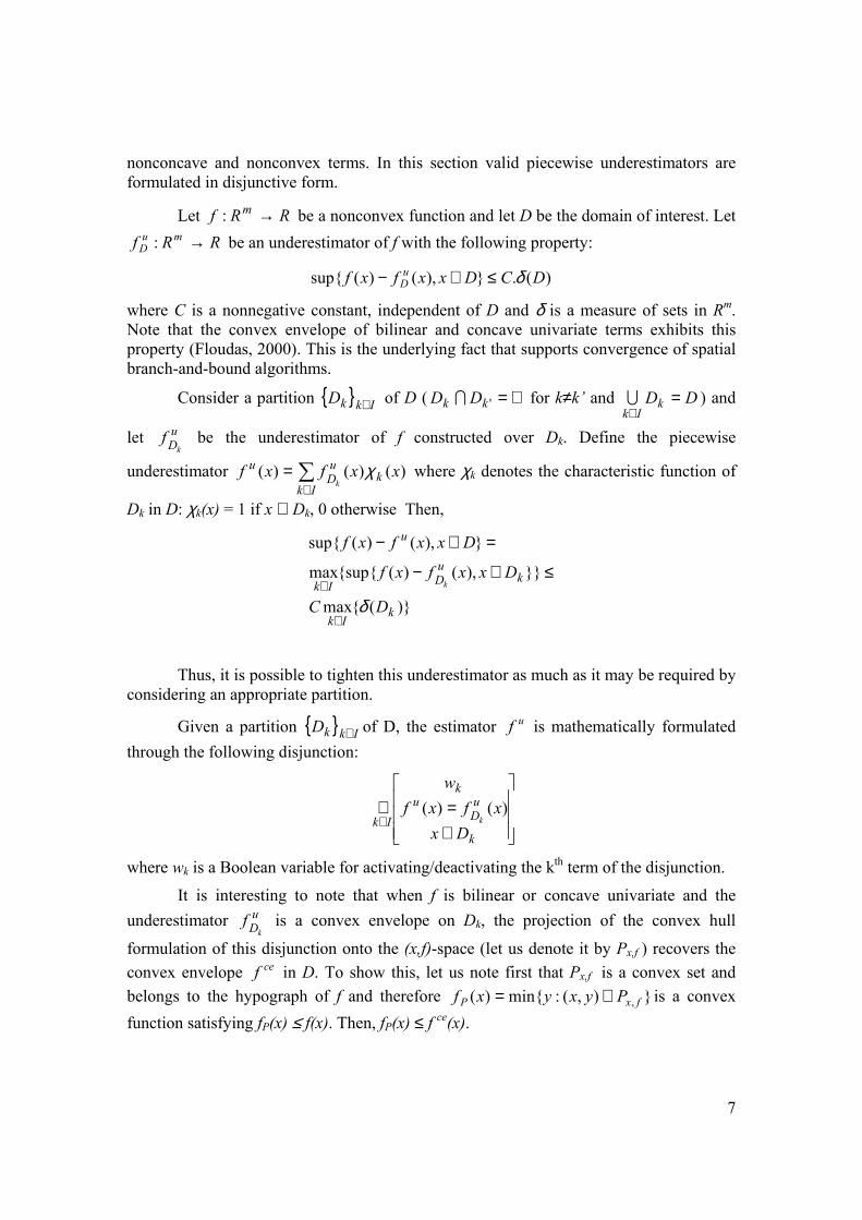
nonconcave and nonconvex terms. In this section valid piecewise underestimators are formulated in disjunctive form.
Let RRf m →: be a nonconvex function and let D be the domain of interest. Let RRf mu
D →: be an underestimator of f with the following property:
)(.),()(sup DCDxxfxf uD δ≤∈−
where C is a nonnegative constant, independent of D and δ is a measure of sets in Rm. Note that the convex envelope of bilinear and concave univariate terms exhibits this property (Floudas, 2000). This is the underlying fact that supports convergence of spatial branch-and-bound algorithms.
Consider a partition IkkD ∈ of D ( ='kk DD I ∅ for k≠k’ and DDkIk
=∈U ) and
let uDk
f be the underestimator of f constructed over Dk. Define the piecewise
underestimator ∑∈
=Ik
kuD
u xxfxfk
)()()( χ where χk denotes the characteristic function of
Dk in D: χk(x) = 1 if x ∈ Dk, 0 otherwise Then,
)(max
),()(supmax
),()(sup
kIk
kuDIk
u
DC
Dxxfxf
Dxxfxf
k
δ∈
∈≤∈−
=∈−
Thus, it is possible to tighten this underestimator as much as it may be required by considering an appropriate partition.
Given a partition IkkD ∈ of D, the estimator uf is mathematically formulated through the following disjunction:
∈=∨
∈k
uD
uk
IkDx
xfxfw
k)()(
where wk is a Boolean variable for activating/deactivating the kth term of the disjunction.
It is interesting to note that when f is bilinear or concave univariate and the underestimator u
Dkf is a convex envelope on Dk, the projection of the convex hull
formulation of this disjunction onto the (x,f)-space (let us denote it by Px,f ) recovers the convex envelope cef in D. To show this, let us note first that Px,f is a convex set and belongs to the hypograph of f and therefore ),(:min)( , fxP Pyxyxf ∈= is a convex function satisfying fP(x) ≤ f(x). Then, fP(x) ≤ f ce(x).

8
Conversely, Px,f contains the sets )),(,( ku
Dk Dxxfxk
∈=φ , for all k∈ I (φk is the projection of the facet defined by wk=1). Actually, Px,f is the convex hull of the union
kIkφ
∈U . Then, since u
Dkf is the convex envelope of f on Dk , φk is contained in the epigraph
of cef , and also Px,f is in it. Then, fP(x) ≥ fce(x).
In the remaining part of this section, the specific piecewise underestimators are obtained.
3.2.a -Univariate Concave Terms. The convex envelope of a univariate concave function over an interval I=[xlo, xup]
is the linear function matching the original one at the extreme points of the interval. The underestimator constructed on a partition KkkI ,...,1= of I (Ik = [xk, xk+1]) is piecewise
linear and matches the function in K+1 points 1,...1 += Kkkx . The mathematical
formulation in terms of mixed-integer linear constraints is (see Appendix A for derivation):
1,0
1
0
)()()(
)(
1
1
1
1
1
∈
=
≤≤
−+=
−+=
∑
∑
∑
=
=
+
=
+
k
K
kk
kk
K
k
kkk
kk
u
K
k
kkk
kk
w
w
w
xfwxff
xwxx
λ
λλ
λλ
3.2.b –Bilinear Terms The convex envelope of bilinear terms on a rectangular domain D is given in
McCormick (1976). It estimates a bilinear function with zero gap in the boundary of D, and the maximum approximation gap depends linearly on the area of D.
Let us consider the bilinear term f(x,y) = xy, defined in the domain D = [xlo, xup]× [ylo, yup], and consider the K+1 points xlo=x1, x2, …, xK+1=xup. In Appendix B the derivation of the piecewise convex underestimator of f over the partition KkkD ,...1= ,
Dk=[xk, xk+1]× [ylo, yup] is presented. The following formulation is obtained,

9
1,0
1
,...,1
,max
...
...
1
11
11
21
21
∈
=
=≤≤
≤≤
−+−+=
+++=
+++=
∑
∑
=
+=
++
k
K
k
k
kupkklo
kkkkk
K
k
kupkkkupkklokkkloku
K
K
w
w
Kkwywy
wxwx
wyxxywyxxyf
y
x
γυ
γυγυ
γγγυυυ
Note that uf = xy when x = xk for some k = 1,…,K+1 or when y = ylo or y = yup.
This formulation provides an underestimation for the bilinear term xy. Overestimation is required for bilinear terms appearing with negative coefficient, that is, -xy. In such a case, the previous formulation is applied to the bilinear term zy, where z = –x.
Also note that the partition is performed in one unique dimension. Partition in both variables is possible, but the formulation requires many more binary and continuous variables.
3.3 Bounding Problem Assume that the functions f, g and h in (O-GDP), after a possible variable
transformation, are expressed as follows,
∑
∑
∑
∈
∈
∈
+=
+=
+=
jHi
ncjijj
Gi
nci
Fi
nci
xhxhxh
xgxgxg
xfxfxf
)()()(
)()()(
)()()(
0
0
0
where f 0, h0, g0 are convex terms and fi nc, hinc, gji
nc are the nonconvex terms (concave univariate or bilinear terms) of the corresponding function. Given a gridpoint set K, the hybrid convex bounding GDP problem is as follows,
Min ZL = ∑j
jc + α
s.t. ∑∈
+≥Fi
fi
o zxf )(α
0)( ≤+ ∑∈ Gi
gi
o zxg
Fiztwxf fi
uKi ∈≤),,(,

10
Giztwxg gi
uKi ∈≤),,(,
=
=
¬
∨
=∈≤
≤+ ∑∈
0
0),,(
0)(
,
j
j
j
jj
jhji
uKji
Hi
hji
oj
j
ctwx
B
Y
cHiztwxh
zxhY
γ
j∈ D
Ω(Y) = True
α∈ R ,x≥0, c≥ 0, Y ∈ True, Falsem zf
i , zgi ,zh
ji∈ R, w∈ 0,1k×s , t∈ Rp×q
(C-GDP)
New variables fiz , g
iz and hijz are added, representing the nonconvex terms in f, g
and hj respectively. uKif , , u
Kig , , and uKjih , are piecewise underestimators of the nonconvex
terms. They are expressed in terms of the original variables x, the new 0-1 variables w and the continuous variables t that are needed for defining the approximation in the grid. The subindex K means that these estimators are constructed using the gridpoint set K. The problem (C-GDP) is a relaxation of (O-GDP), and therefore the optimal solution of (C-GDP) is a lower bound to the solution of (O-GDP).
The following theorem is important to validate the algorithm:
Theorem: If the optimal solution of (C-GDP) belongs to the set of grid points, this corresponds to the global solution of (O-GDP).
Proof: Let us denote (x*, w*, t*, Y*) the optimal point in (C-GDP) and assume x* is a grid point. Thus, the piecewise underestimators have zero gap in x*, that is:
)(),,( ****, xftwxf iuKi = for i∈ F, )(),,( ****
, xgtwxg iu
Ki = i∈ G, and
)(),,( ****, xhtwxh ji
uKji = for i∈ Hj and Yj
*=True. Moreover, Bj(x*, w*, t*)T=0 for Yj
*=False. Therefore, (x*,Y*) is feasible in (O-GDP). Since x* is an optimal point, the first and third global constraints in (C-GDP) are active, and
∑∈
+=Fi
uKi
o twxfxf ),,()( ***,
*α . Thus,
****
***,
**
)()()(
),,()(
∑ ∑∑
∑∑∑
∈
∈
=+=++
=++=+=
Fi jji
o
jj
Fi
uKi
o
jj
jj
L
Zxfcxfxfc
twxfxfccZ α
This proves that the optimal objective value of (C-GDP) is equal to the objective value in a feasible point in (O-GDP). Since the (C-GDP) problem is a relaxation of the (O-GDP), Z* is the best value for the objective in (O-GDP).

11
It should be noted, however, that if the global optimum of (O-GDP) is a grid point of (C-GDP), this point might not be the optimum of (C-GDP), due to the underestimation gap.
The disjunctive problem (C-GDP) is then linearized using supporting hyperplanes derived at solution points, similarly as in the OA algorithm, and converted into an MILP problem, by formulating the convex hull representation of the disjunctions and replacing the boolean variables with binary variables y. The resulting MILP has binary variables of two different types: the variables w, introduced in the piecewise underestimators, and the variables y denoting the existence of units. Let us denote this problem (MILP-1).
Assume that L subproblems (R-NLP) have been solved, with solution points ,...,1, Llxl = . The convex part of the objective function and the global constraints are
linearized in such L points. The convex part of the constraints in disjunction j is linearized in the subset of points , jl Llx ∈ , where Lj is the set of iterations with Yj=True. Specifically, the problem (MILP-1) is constructed as follows,
Min ZL = ∑
jjc + α
s.t. ∑∈
+−∇+≥Fi
fi
llolo zxxxfxf ))(()(α
0))(()( ≤+−∇+ ∑∈ Gi
gi
llolo zxxxgxg Ll ,...,1=
Fiztwxf fi
uKi ∈≤),,(,
Giztwxg gi
uKi ∈≤),,(,
=
=
¬
∨
=∈≤
∈≤−∇+ ∑∈
0
0),,(
0))(()(
,
j
j
j
jj
jhji
uKji
j
Hi
hji
lloj
loj
j
ctwx
B
Y
cHiztwxh
LlzxxxhxhY
γ
j∈ D
Ω(Y) = True
α∈ R ,x≥0, c≥ 0, Y ∈ True, Falsem zf
i , zgi ,zh
ji∈ R, w∈ 0,1k×s , t∈ Rp×q
(MILP-1)
4. Reduced NLP
Reduced NLP (R-NLP) problems are solved iteratively with the master problem. Similarly to the Logic-Based OA, these NLPs are reduced, in the sense that fixing the Boolean variables means that a set of continuous variables (those related to nonexistent units) is set to zero and removed from the NLP, as well as the constraints modeling those

12
units. The NLPs have to be solved to global optimality. Having fixed unit configurations in the network allows us to contract the bounds, and therefore reduce the search region.
In order to solve (R-NLP) to global optimality, the algorithm relies on the local lower bounding problem (C-MINLP). This problem is obtained from (C-GDP) by fixing the boolean variables Yj or, in other way, by introducing the piecewise underestimators in (R-NLP). The local bounding problem is as follows,
Min Z = ∑
jjc + α
s.t. ∑∈
+≥Fi
uKi
o twxfxf ),,()( ,α
0),,()( , ≤+∑∈ Gi
uKi
o twxgxg
TrueYc
twxhxhj
jj
Hi
uKji
oj
j =
=
≤+ ∑∈
γ
0),,()( ,
FalseY
ctwx
Bj
j
j
=
=
=
0
0
α∈ R ,x∈ Rn, c≥ 0,
w∈ 0,1k×s , t∈ Rp×q
(C-MINLP)
Let us denote by (MILP-2) the MILP problem that is the linearization of the problem (C-MINLP). Note that (MILP-2) is also obtained by fixing the binary variables y in (MILP-1).
In Figure 2 the relation between the different previously defined problems is shown. Upper bounding problems are obtained by moving to the right in the figure. Lower bounding problems appear by moving down.
Note that in some cases some simplifications are possible. For example, in bilinear programs, (C-GDP) is the same as (MILP-1) and (C-MINLP) is the same as (MILP-2), since there are no nonlinear convex terms in the original problem or any possible variable transformation. Certainly, if the original problem is convex, problems (O-GDP) and (C-GDP), and problems (R-NLP) and (C-MINLP) are identical. It may also be the case that, although the original problem is nonconvex, a convex NLP arises by fixing the boolean variables. In such a case, (R-NLP) and (C-MINLP) are the same problem, perhaps in different variable spaces (e.g. Geometric Programs).

13
5. Algorithm
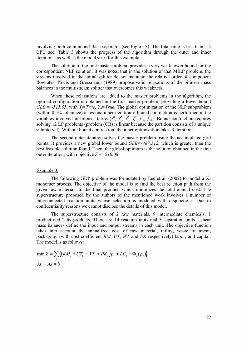
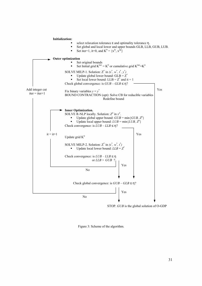
The algorithm has two main phases as can be seen in Fig. 3:
Outer Optimization: This phase calculates a global lower bound (GLB) of the optimum of problem (O-GDP). The problem (MILP-1) is solved using an initial grid and initial linearization points, to predict a new structure in the network and a new global lower bound. An increasing sequence of global lower bounds is obtained in the successive iterations of this phase. This is true because (MILP-1) is modified by adding integer cuts in Yj that avoid repeating structures and supporting hyperplanes of the convex functions.
The initial grid can be redefined when solving (MILP-1) or it can accumulate the grid points generated during the inner optimization. The cumulative option has the disadvantage of exponentially increasing the size of the model (MILP-1), making it very difficult to solve. Both alternatives are implemented in the numerical examples.
Inner Optimization: A fixed structure is globally optimized. This is performed by iteratively solving the problems (R-NLP) and (MILP-2) that bound the global solution of the reduced NLP.
Solutions of (R-NLP) provide feasible solutions of (O-GDP), and allow to update the local and global upper bound (LUB and GUB respectively). Tighter local lower bounds (LLB) arise refining the grid and solving the local bounding problem (MILP-2), which is actually a relaxation of (R-NLP).
There may be cases where fixing the boolean variables Y, the resulting NLP problem is convex, or it is known that it has a unique optimal solution. An example of this kind of problem is the GDP model for the synthesis and design of a batch plant formulated by Lee and Grossmann (2001). In such cases, the inner optimization can be accomplished by simply solving the problem (R-NLP) with a local solver.
Alternatively, one might resort to a global NLP optimizer (e.g. BARON, Sahinidis, 1996) that will take advantage of the tighter variable bounds that arise in a fixed configuration.
Bound Contraction: Since the elimination of non-optimal subregions is crucial in accelerating the search, an optional bound contraction procedure is considered in order to reduce the search space in the global optimization of the NLP subproblems. This contraction is performed before the algorithm enters in the inner optimization phase. The scheme for contraction adopted in this work is the same as the one proposed by Zamora and Grossmann (1999). Basically, the problem solved at each contraction step is the following,
min/max xi
s.t Z ≤ GUB
constraints in C-MINLP
(CB)
This problem is a convex problem whose feasible region overestimates the subregion of (R-NLP) where the objective function can be improved. The aim of this

14
problem is to eliminate part of the original feasible region where the global optimum does not exist.
Note that in general, (CB) is a MINLP problem, since binary variables w related to the initial grid are involved. However, if the initial grid consists of only variable bounds and therefore the original domain is not really subdivided, (CB) can be solved as an NLP.
The bound contraction is performed on those variables that are involved in the relaxation so that the underestimators can be tightened.
Grid Update: The grid is updated for each nonconvex term. The idea in refining the grid is to include in it those points obtained as optimal points in the relaxed problem.
The decision of adding a new point to the grid is based on the error between the
nonconvex term nciζ and the substituting variable ζ
iz in the solution ),(∗∗ ζ
izx of (MILP-1) or (MILP-2) where ζ = f, g or h. The following criterion is adopted:
If nci
ncii xz ζεζζ >− ∗∗
)( , then add x* to the grid corresponding to nciζ , where ε is a
specified tolerance.
An alternative strategy for updating the grid is to include in it the middle point of
the active subinterval in the solution of the master problem. If the solution ),(∗∗ ζ
izx of
the master problem is such that 1* +≤≤ kk xxx (interval k is active) then, the grid
corresponding to nciζ is modified by adding the point
2
1++ kk xx .
Convergence: The proposed underestimators are constructed over a partition of the domain, and they involve an approximation error that depends on the size of each subdomain. Then, as the dimension of the subdomains is reduced by further partitions, the gap of approximation is also reduced.
6. Illustrative Example.
Let us consider again the illustrative example discussed in section 2.
The proposed algorithm starts solving the MILP obtained by replacing the concave constraint in the third disjunction with the piecewise linear relaxation constructed over the interval defined by the bounds of x5 and replacing the disjunctions with their convex hull reformulation. This first master problem MILP-1 predicts the lower bound GLB = 25.19, with Y=True, False, True with x5
*=1, x6*
=7.67 (see Figure 4). The NLP subproblem corresponding to these boolean values predicts an upper bound GUB= 35.91. Since there is a gap between the lower and upper bounds, the problem MILP-2 is solved, including x5
* in the grid. This problem has an optimal solution Z
=35.91 with x5*
= 1 and x6*
= 1.72, which in fact is the global optimum of this configuration.

15
In the second outer iteration, the new global lower bound obtained is GLB=36.38, with Y=False, True, True. This bound is greater than the best known solution, therefore the algorithm stops with the global solution Z =35.91.
7. Numerical Examples:
The proposed algorithm was implemented in GAMS (Brooke et al, 1997) and 5 examples were solved on a 1.8 GHz Pentium 4 PC with 256 Mbytes memory. GAMS/CONOPT2 and GAMS/BARON 5.0 (Sahinidis, 1996) were used with their default options to solve the reduced NLP problems, and GAMS/CPLEX 8.1 for the MILP problems.
Example 1: A process network problem, which is a variation of the problem in Duran and
Grossmann (1986) was solved using the proposed algorithm. The problem involves 8 processes, with 25 flow streams (Fig. 5). The objective function to be minimized considers fixed costs cj for selected units and operating costs for stream xi, with coefficients pi . The GDP formulation of the model is as follows:
22121
21919
21010
233
222
8
1
)2.1(5.010)3(
)4(3.015)7.0()3(122min
−−+−
−−−+−+−−++ ∑∑∈=
xpxp
xpxpxpxpcLi
iij
j
s.t.
00
00
00
00
241423
222023
876
151211
2516917
211913
11653
421
=−−=−−
=−−=−−
=−−−=−−
=−−−=−−
xxxxxx
xxxxxx
xxxxxxx
xxxxxxx
0205
04.008.0
1412
1412
1710
1710
≥−≤−
≥−≤−
xxxx
xxxx
===
¬∨
=≤−−
00
2501
1
23
1
1
2
13
cxxY
cxe
Yx

16
===
¬∨
=≤−−
00
4001
2
45
2
2
42.1
25
cxxY
cxe
Yx
====
¬∨
==+−
00
3005.1
3
1089
3
3
1089
3
cxxx
Y
cxxx
Y
====
¬∨
==−
00
50025.1
4
141213
4
4
131412
4
cxxx
Y
cxxx
Y
===
¬∨
=≤−
00
3002
5
1615
5
5
1615
5
cxxY
cxx
Y
===
¬∨
=≤−−
00
3501
6
1920
6
6
195.1
620
cxxY
cxe
Yx
===
¬∨
=≤−−
00
2001
7
2122
7
7
21
722
cxxY
cxe
Yx
====
¬∨
=≤−−−
00
2501
8
171018
8
8
1710
818
cxxx
Y
cxxe
Yx
54
76
YYYY
¬∨¬¬∨¬
xi , cj ≥ 0, Yj ∈ True, False, i=1, 2, …,25, j=1, 2,…, 8
When the Logic-Based OA algorithm by Türkay and Grossmann (1996) is applied in this problem, using the termination criterion of no improvement in the objective of the NLP solutions, it stops in the third major iteration with a suboptimal solution Z =10.627. Also, none of the master solutions is lower than the global optimum. If the termination criterion is not applied and we let the algorithm continue iterating, the global solution is found in major iteration 18. However, there is no guarantee of globality.
The problem was also formulated as an MINLP using the Big-M formulation of the disjunctions (with M=100) and solved using the GAMS/DICOPT solver, which

17
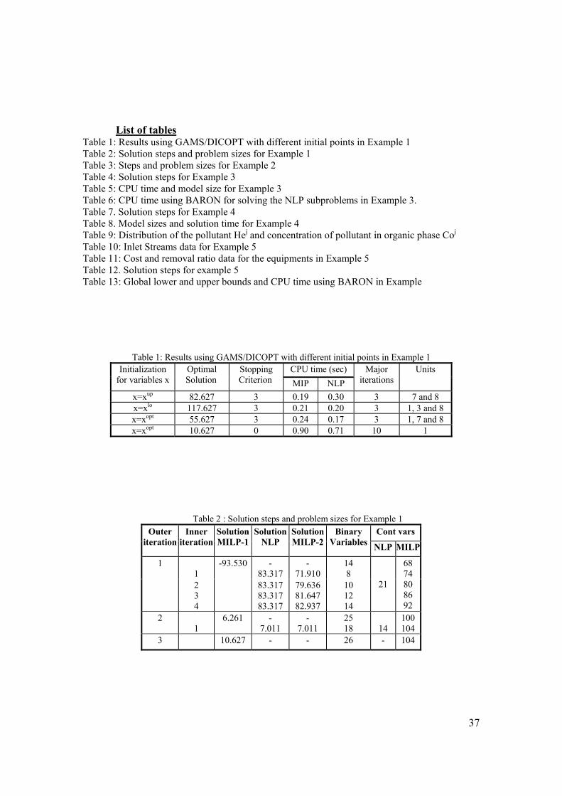
implements the AP/OA/ER algorithm (Viswanathan and Grossmann, 1990). The solution depends strongly on the initial point. Several initial points were used, but none of the runs finds the global solution. Some results are shown in Table 1. Using the stopping criterion 3, DICOPT stops when the solutions of the NLP subproblems have no improvement, and the stopping criterion 0 forces DICOPT to continue performing a specified number of iterations (10 iteration in the results of Table 1)
The algorithm proposed in this work obtains the optimal structure (units 1,4,7) in two outer iterations. The configuration obtained in the first master (MILP-1) consists of units 1, 3, 4, 7 and 8, and the lower bound is GLB = -93.53. This structure is optimized in 4 inner iterations. The corresponding (MILP-2) subproblems are set up adding in the grid the variable values obtained in the optimal solution of the master problem, and adding the linearizations of the convex term in the solution of the NLP subproblem. An integer cut is added in order to make this configuration infeasible in subsequent master problems. The gridpoint set is updated by simply adding the new point to the grid of the previous iteration.
The optimal structure with objective f=7.011 and involving units 1, 4 and 7 is selected in the next outer iteration, and it requires one inner iteration to prove globality in the solution of the subproblem. One additional outer iteration is required to check convergence to the global optimum.
The algorithm requires less than 1 CPU sec in solving the MILP subproblem and 0.5 CPU sec in solving the NLP subproblems. Details of the solution steps and problem sizes can be seen in Table 2. The problem was also solved with BARON (Sahinidis, 1996), which required 0.3 CPU-sec and 25 nodes in the branch-and-bound tree, yielding the same solution of f=7.011.
Example 2:
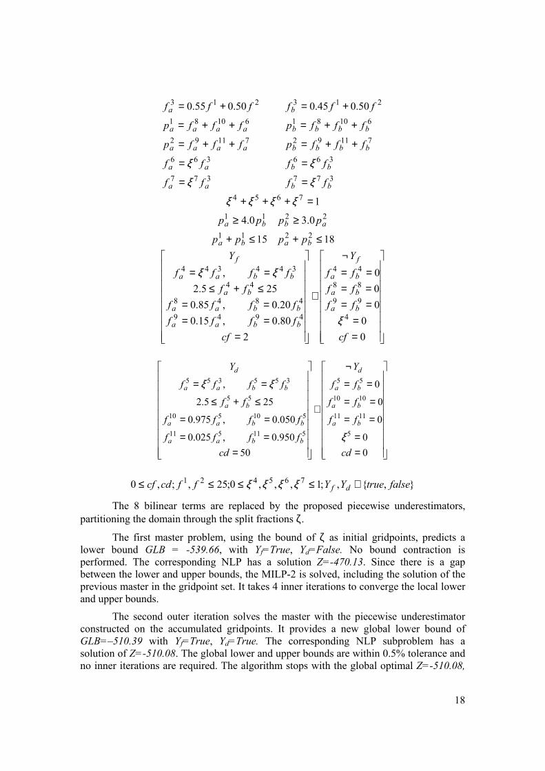
The next example was taken from Kocis and Grossmann (1989). It involves the selection of the optimal separation scheme to be used to separate a multicomponent process stream into a set of product streams with given purity specifications. The superstructure consists of feed and product mixers, two possible separation units and a splitter that splits the feed into streams towards the separators or towards the final mixers (Figure 6). The alternative schemes include the use of flash separation, distillation, or the elimination of the complete separation process if it is proven to be unprofitable. The nonconvex (bilinear) GDP model for this problem is as follows,
Min cdcfffffffppz bababa ++++++++−−= 55442121 448103035
18
1815
0.30.4
1
50.045.050.055.0
2211
2211
7654
377
366
71192
61081
213
377
366
71192
61081
213
≤+≤+
≥≥
=+++
=
=
++=
++=
+=
=
=
++=
++=
+=
baba
abba
bb
bb
bbbb
bbbb
b
aa
aa
aaaa
aaaa
a
pppp
pppp
ff
ff
fffp
fffp
fff
ff
ff
fffp
fffp
fff
ξξξξ
ξ
ξ
ξ
ξ
==
======
¬
∨
=====
≤+≤==
00
000
280.0,15.020.0,85.0
255.2,
4
99
88
44
4949
4848
44
344344
cf
ffffffY
cfffffffff
ffffff
Y
ba
ba
ba
f
bbaa
bbaa
ba
bbaa
f
ξ
ξξ
5 5 3 5 5 3 5 5
5 5 10 10
10 5 10 5 11 11
11 5 11 5 5
, 0
2.5 25 0
0.975 , 0.050 0
0.025 , 0.950 050 0
d d
a a b b a b
a b a b
a a b b a b
a a b b
Y Y
f f f f f f
f f f f
f f f f f f
f f f fcd cd
ξ ξ
ξ
¬
= = = = ≤ + ≤ = = ∨ = = = = = = =
= =
,,;1,,,0;25,;,0 765421 falsetrueYYffcdcf df ∈≤≤≤≤ ξξξξ
The 8 bilinear terms are replaced by the proposed piecewise underestimators, partitioning the domain through the split fractions ζ.
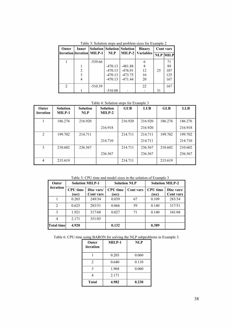
The first master problem, using the bound of ζ as initial gridpoints, predicts a lower bound GLB = -539.66, with Yf=True, Yd=False. No bound contraction is performed. The corresponding NLP has a solution Z=-470.13. Since there is a gap between the lower and upper bounds, the MILP-2 is solved, including the solution of the previous master in the gridpoint set. It takes 4 inner iterations to converge the local lower and upper bounds.
The second outer iteration solves the master with the piecewise underestimator constructed on the accumulated gridpoints. It provides a new global lower bound of GLB=–510.39 with Yf=True, Yd=True. The corresponding NLP subproblem has a solution of Z=-510.08. The global lower and upper bounds are within 0.5% tolerance and no inner iterations are required. The algorithm stops with the global optimal Z=-510.08,
19
involving both column and flash separator (see Figure 7). The total time is less than 1.5 CPU sec. Table 3 shows the progress of the algorithm through the outer and inner iterations, as well as the model sizes for this example.
The solution of the first master problem provides a very weak lower bound for the correspondent NLP solution. It was noted that in the solution of that MILP problem, the streams involved in the initial splitter do not maintain the relative order of component flowrates. Kocis and Grossmann (1989) propose valid relaxations of the bilinear mass balances in the multistream splitter that overcomes this weakness.
When these relaxations are added to the master problems in the algorithm, the optimal configuration is obtained in the first master problem, providing a lower bound GLB = -515.55, with Yf=True, Yd=True. The global optimization of the NLP subproblem (within 0.5% tolerance) takes one inner iteration if bound contraction is performed in the variables involved in bilinear terms (ζ4, ζ5, ζ6, ζ7, f3
a, f3b). Bound contraction requires
solving 12 LP problems (problem (CB) is linear because the partition consists of a unique subinterval). Without bound contraction, the inner optimization takes 3 iterations.
The second outer iteration solves the master problem using the accumulated grid points. It provides a new global lower bound GLB=-487.512, which is greater than the best feasible solution found. Then, the global optimum is the solution obtained in the first outer iteration, with objective Z = -510.08.
Example 3.
The following GDP problem was formulated by Lee et al. (2002) to model a X-monomer process. The objective of the model is to find the best reaction path from the given raw materials to the final product, which minimizes the total annual cost. The superstructure proposed by the authors of the mentioned work involves a number of interconnected reaction units whose selection is modeled with disjunctions. Due to confidentiality reasons we cannot disclose the details of this model.
The superstructure consists of 2 raw materials, 8 intermediate chemicals, 1 product and 2 by-products. There are 14 reaction units and 3 separation units. Linear mass balances define the input and output streams in each unit. The objective function takes into account the annualized cost of raw material, utility, waste treatment, packaging, (with cost coefficient RM, UT, WT and PK respectively) labor, and capital. The model is as follows:
( ) ∑ Φ+++++=
iiiiiiiii pLCpPKWTUTRMZ )(min
bAxts =..

20
TrueY
Ii
LCp
x
x
Y
XUBpxx
LCxp
xxYield
Y
i
i
OUTi
INi
i
iOUTi
INi
ii
OUTii
OUTi
INii
i
=Ω
∈∀
==
=
=
¬
∨
≤≤
==
=×
)(
,
00
0
0
,,0
α
IifalsetrueYIiLC
NnIiXUBpxxx
i
i
iOUTi
INin
∈∀∈∈∀≤
∈∀∈∀≤≤
,,,0
,,,,,0
I denotes the set of units and N the set of chemicals. The variables xn represents the molar flowrate of component n, and xi
IN and xiOUT are the inlet and oulet flowrates in
unit i. The production of each unit is represented with pi. It is assumed that the conversion of unit i, Yieldi, is given.
The capital cost Φi(pi) is a concave function of the production rate. The master problems are set up replacing each of these terms with a variable bounded by the piecewise linear underestimator.
GAMS/DICOPT solves the Big-M reformulation of this problem providing a local solution Z =246.342 M$/yr, for a production of 450 Mlb/yr of X-monomer and no by-product production. This solution involves 7 reaction units and 2 separation units. DICOPT stops with worsening of the NLP solutions at the second major iteration. If we allow the solver to go on the search until a maximum of 20 major iteration, the best found solution is Z =242.760 and none of the master objective is below this value.
The global optimal reaction path involves 5 reaction units and 2 separation units (see Figure 8). The production of X-monomer is 450 Mlb/yr with a by-product production of 26.1 Mlb/yr. The total annual cost is 214.711 M$/yr.
The sequence of steps for obtaining the global solution using the proposed algorithm is shown in Table 4, as well as the progress of the lower and upper bounds. No bound contraction was performed. Four outer iterations were required to obtain a global lower bound greater than the best feasible solution. Each NLP subproblem was solved to global optimality in one inner iteration and the gridpoint sets were updated with the solution of the MILP problems. The grid was not reset in the outer iterations but it accumulated all the added points. Table 5 shows the CPU time required in each step and the size of each solved subproblem. Note that the total CPU time used is 5.441 sec.
This example was also solved using GAMS/BARON in two ways. In the first one BARON was used to solve the NLP subproblems to global optimality instead of performing the inner loop in Fig. 3. The optimal objective values obtained with this alternative are the same as shown in Table 4 for the problems (MILP-1) and NLP subproblems and the CPU time are shown in Table 6. As can be seen the CPU-time is slightly lower (5.212 sec vs. 5.441 sec). The second way that BARON was used was to

21
directly solve the full problem O-GBD (its Big-M reformulation). In this case BARON could not solve the problem O-GDP in less than 960 sec. At that point, the search was interrupted, and the lower bound that BARON provided (109.018) was about 50% below the global optimal solution (214.711).
Example 4:
This example corresponds to a synthesis problem of a distributed wastewater multicomponent network, which is taken from example 10 of Galan and Grossmann (1998). Given a set of process liquid streams with known composition, a set of technologies for the removal of pollutants, and a set of mixers and splitters, the objective is to find the interconnections of the technologies and their flowrates to meet the specified discharge composition of pollutant at minimum total cost. Discrete choices involve deciding what equipment to use for each treatment unit. Lee and Grossmann (2001) formulated the problem as a GDP model.
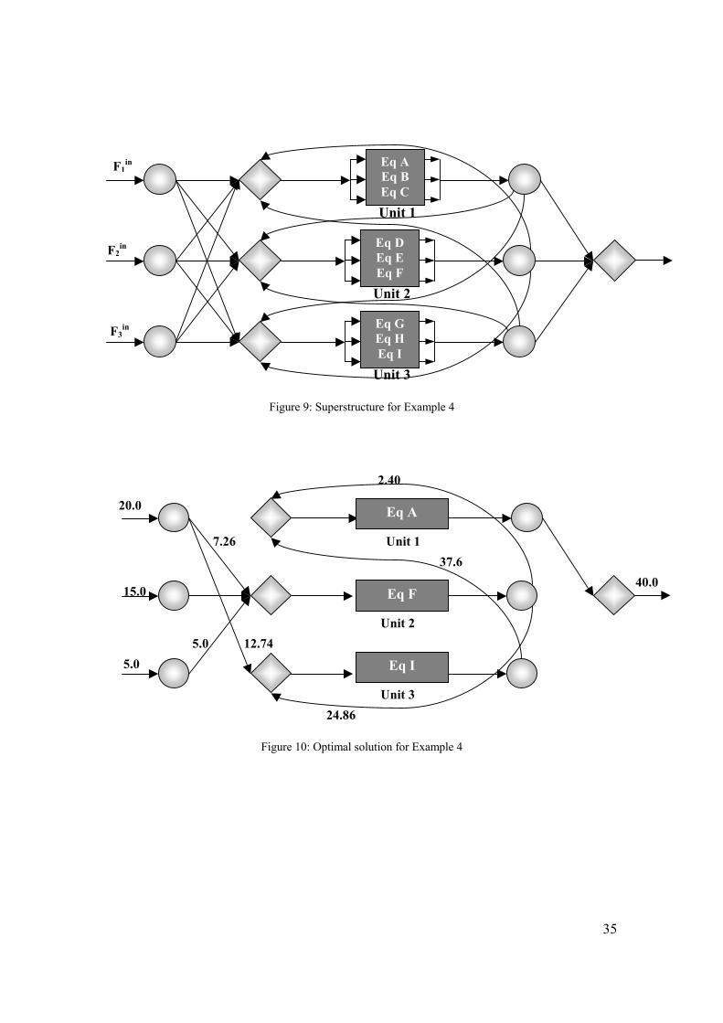
The superstructure is shown in Figure 9, involving three inlet streams, which are split into streams going into the treatment units. There are three different equipment available for removal of each of the pollutants. Each equipment has different removal ratio of the pollutants and cost function. The outlet stream of each treatment unit is again split and then a fraction of the stream is recycled, while the rest of the stream is sent to the final mixer for discharge. The data for this example are given in Lee and Grossmann (2001).
The nonlinearities in this model are due to the bilinearities that arise in the component mass balances in the final splitters and the concave cost functions.
This problem was solved to global optimality with our algorithm in just under 2 min. Bound reduction was performed in the complicating variables representing the total flows in the treatment units. These variables are involved in the bilinear mass balances in the final splitters. The initial grid for the outer iterations was set up with three points: the lower and upper bounds and the middle point. Within each inner iteration, the gridpoint sets were updated using the middle point of the active subinterval. Adding the master solution point to the grid causes slower convergence to the global solution of the reduced NLP.
The global optimum solution is shown in Figure 10. Six outer iterations were necessary to prove globality of the solution as seen in Table 7. In the third outer iteration, (MILP-1) selected the optimal equipment, and obtained a lower bound within a tolerance of 0.5% requiring 5 iterations in the inner optimization. Table 8 shows the computing times and the problem sizes. The total time required by the algorithm was 11.31 sec for solving the (MILP-1) problems, 0.54 sec for solving (R-NLP) subproblems, 8 sec for reducing bounds in total flows and 117.56 sec in solving the (MILP-2) subproblems.
The most time consuming step in this example is the inner optimization of the optimal structure. Due to the bound contraction procedure, the reduced NLP could be solved to global optimality with the solver BARON 6.0. It rapidly detected the infeasibility of the first two NLP subproblems. In the third equipment selection, BARON

22
found the global optimum of the NLP in 20 CPU sec. The MILP-1 problems in the following outer iterations detected infeasible structures. The total time required with this implementation of the method was approximately 38 CPU sec, which is considerably lower than the 118 secs with the algorithm of Fig. 3.
Example 5:
The next example is a wastewater treatment network problem, where the separation is performed using nondispersive solvent extraction (NDSX) (see Galan and Grossmann, 1998). For NDSX technologies, the outlet concentration depends on the inlet concentration of the pollutant and on the flow rate. However, the flowrate of the inlet stream is assumed not to change during the treatment, since the concentration of the pollutants is low. A short-cut model of the NDSX is used. The equation for the NDSX treatment is as follows
))(.exp( jjjtjjj CoceHeFLOWT
NMKmHeaCocsHe −−=−
where csj is the outlet concentration of pollutant j, cej is the inlet concentration of j, at is the surface area of the hollow fiber module (135 m2), NM is the number of modules, Km is the membrane transport coefficient (a value of 2.2 10-8 m/s was used), Hej is the distribution constant of the pollutant between the organic phase and the aqueous phase, and Coj is the concentration of the contaminant in the organic phase. In the simplified case, where extraction and back-extraction are carried out at the same rate, we can assume that Coj remains constant.
The superstructure for this problem is identical to example 4. The data for the equipment, inlet streams and costs are shown in Tables 9, 10 and 11.
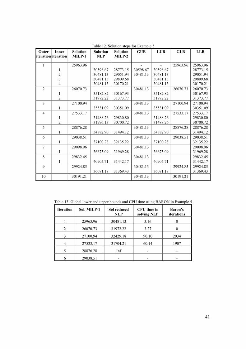
The global optimum ($30,481.13) was found in the first outer iteration, but the convergence within 1% tolerance of the global optimum was obtained in 10 outer iterations. The first selected structure required 4 inner iterations each to check globality. The gridpoint sets were updated in each inner optimization using the middle point of the active subinterval. Details of the solution in each iteration can be seen in Table 12, as well as the global and local lower and upper bounds. Figure 11 shows the progress of the bounds. Note that the global lower bound defines a piecewise increasing path, and the global upper bounds describes a piecewise decreasing path, always above the global lower bound line. This does not occur with the local bounds. Local bounds involve discontinuities when the inner loop finishes and outer iteration changes. Also note that inner loop stops if the local lower bound reaches the global local bound.
(MILP-1) problems have 51 binary and 790 continuous variables, whilst the (MILP-2) problems have on average 60 binary variables and 973 continuous variables in the first inner iteration, and their size grow as the inner iterations proceed. The fourth (MILP-2) in outer iteration 1 has 114 binary variables and 1522 continuous variables. The time required to solve the 10 outer master problems is 0.33 min aproximately; the bound reduction steps take a total of 0.83 min. The algorithm spends 2.5 sec in solving the NLPs problems and 18 min in solving the bounding problems (MILP-1). The optimal values for the flows are shown in Figure 12 (flow values are given in ton/h)

23
Numerical difficulties were experienced with BARON, which prevented convergence to feasible solutions, and hence a comparison of computational times was not possible for this problem.
8. Conclusions and future works.
A new deterministic algorithm for the global optimization of synthesis of processes network problems has been presented. It is based on a new methodology for constructing underestimators of nonconvex functions based on partitions of the entire domain. In this work, the derivation of this class of estimators for univariate concave terms and bilinear terms has been developed.
The proposed algorithm relies on an outer approximation methodology. The global solution of the problem is achieved by solving problems that are relaxations of the original one. As iterations proceed, the bounding problem approximates the original problem with more accuracy.
The effectiveness of the proposed algorithm has been illustrated in several examples as well as comparisons with other existent algorithm to solve this class of problems. The computational experience, although still limited, suggests that this algorithm has several advantages with respect to spatial branch-and-bound algorithms, particularly in regard to ease of implementation and potential strengthening of lower bounds.
For larger problems, however, the relaxed MILP problems predict bounds with significant gap and convergence is achieved at high computational cost. A modification of the algorithm is being studied, involving the solution of the convexified C-MINLP problem. Also, most of the computing time is spent in the inner optimization. This is due to the iterative procedure and the increasing size of the MILP-2 problems. An alternative methodology for obtaining the global solution of the reduced NLPs is also being investigated. It involves the simultaneous grid update and solution of the local bounding problem.
Acknowledgment. The authors would like to acknowledge financial support from CONICET, ANCyT and UNL from Argentina, the Center for Advanced Process Decision-making at Carnegie Mellon, and the National Science Foundation under grant INT-0104315.
References
Adjman C.S., Androulakis I.P. and Floudas C.A., “Global Optimization of Mixed-Integer Nonlinear Problems. AIChE Journal, 46(9), 1769-1797, 2000
M.S. Bazaraa, H.D. Sherali and C.M. Shetty. Nonlinear Programming, Theory and Algorithms, second edition. Wiley, New York, 1993.
Björn K.M., Lindberg P.O., Westerlund T., “Some convexifications in global optimization of problems containing signomial terms”, Comp and Chem Engng, 27, 669, 2003

24
Brooke A., D. Kendrick, A. Meeraus and R. Raman, GAMS Language Guide, Release 2.25, Version 92. GAMS Development Corporation, 1997.
Duran M.A. and Grossmann I.E., “An Outer-Approximation Algorithm for a Class of Mixed-Integer Nonlinear Programms”, Math Programming 36, 307, 1986
Fletcher R. and Leyffer S., “Solving mixed Integer nonlinear programs by outer approximation”, Math Programming, 66, 550, 1994
Floudas C.A., “Deterministic Global Optimization: Theory, Methods and Applications, Kluwer Academic Publishers: Dordrecht, The Netherlands, 2000
Galan B. and Grossmann I.E., “Optimal Design of Distributed Wastewater Treatment Networks”. Industrial and Engineering Chemistry Research, 37(10), 4036, 1998.
Geoffrion A.M., “Generalized Benders Decomposition”, Journal of Optimization Theory and Applications, 10(4) 237, 1972
Grossmann, I., “Review of Nonlinear Mixed-Integer and Disjunctive Programming Techniques”, Optimization and Engineering, 3, 227, 2002.
Hooker N. and Osorio M.A., “Mixed logical/linear programming”, Discrete Applied Mathematics 96/97, 395 1999
Horst R. and Tuy P.M., “Global Optimization: deterministic approaches”, 3rd edn, Springer-Verlag: Berlin, 1996
Kesavan P. and Barton P.I., “Generalized Branch and Cut framework for mixed-integer Nonlinear Optimization Programs” Comp and Chem Engng, 24, 1361, 2000
Kocis G.R. and Grossmann I.E., “Relaxation Strategy for the structural optimization of Process Flow Sheets”, Industrial and Engineering Chemistry Research, 26,1869, 1987
Lee, S., R.D. Colberg, J. J. Siirola and I.E. Grossmann, “Global Optimization of Disjunctive Program for the Superstructure of an Industrial Monomer Process," Annual Meeting AIChE, Indianapolis, 2002.
Lee S. and Grossmann I.E., “A global optimization algorithm for nonconvex Generalized Disjuntive Programming and Applications to Process Systems”, Comp and Chem Engng, 25 1675, 2001.
Lee S. and Grossmann I.E., “Global optimization for nonlinear Generalized Disjunctive Programming with Bilinear Equality constraints: Applications to Process Networks”, Comp and Chem Engng,27(11) 1557 2003
McCormick G.P., “Computability of global solutions to factorable nonconvex programs-Part I. Convex underestimating problems”, Mathematical Programming. 10, 146, 1976.
Nemhauser and Wosley. “Integer and Combinatorial Optimization”. John Wiley and Son. New York, 1999.
Padberg M. “Approximating separable nonlinear functions via mixed zero-one programs”. Operations Research Letters, 1, 2000.
Pörn, Björn and Westerlund, “Global Solution of Optimization Problems with Signomial Parts, submitted to Optimization and Engineering, 2002
Quesada I. and Grossmann I.E., “A Global Optimization algorithm for linear fractional and bilinear programs”, Journal of Global Optimization, 6, 39, 1995

25
Ryoo and Sahinidis N., “Global Optimization of nonconvex NLPs and MINLPs with applications in Process Design”, Comp and Chem Engng, 19(5), 551, 1995
Sahinidis N., “BARON: a general purpose global optimization software package” Journal of Global Optimization, 8(2), 201, 1996
Smith E.M.B. and Pantelides C.C., “A symbolic reformulation/spatial branch and bound algorithm for the global optimization of nonconvex MINLPs”, Comp Chem Engng, 23,457, 1999
Stubbs R.A. and Mehrotra S, “A Branch and Cut Method for 0-1 Mixed Convex Programming”, Mathematical Programming, 86(3),515, 1999
Tawarmalani M. and Sahinidis N., “Global Optimization of Mixed-Integer Nonlinear Programs: A theoretical and Computational Study”, submitted to Mathematical Programming 2000
Tawarmalani M. and Sahinidis N., “Convexification and Global Optimization in continuous and Mixed-Integer Nonlinear Programming”, Kluwer 2002
Türkay M. and Grossmann I.E., “Logic-Based MINLP Algorithm for the Optimal Synthesis of Process Networks”, Comp and Chem Engng, 20, 959, 1996
Vecchietti A. and Grossmann I.E., “LOGMIP: a Disjunctive 0-1 nonlinear Optimizer for Process System Models”. Comp and Chem Engng, 23,555, 1999
Viswanathan and Grossmann, “A Combined Penalty Function and Outer Approximation Method for MINLP Optimization”, Comp and Chem Engng, 14, 769, 1990
Visweswaran and Floudas, “New Reformulations and branching strategies for the GOP algorithm” in Global Optimization in Engineering Design, ed I.E. Grossmann, Kluwer, 1996
Westerlund and Petterson, “A cutting plane Method for Solving Convex MINLP Problems”, Comp and Chem Engng, 19, S131-S136, 1995
Zamora J.M. and Grossmann I.E., “A branch and contract algorithm for problems with concave univariate, bilinear and linear fractional terms”, Journal of Global Optimization, 14, 217, 1999

26
Appendix A: Derivation of piecewise linear underestimators of concave univariate functions.
The convex envelope of a concave function on an interval I=[xlo, xup] is )()1()()( uplou xfxfxf λλ −+=
where λ is such that uplo xxx )1( λλ −+= .
Given the partition KkkI 1= , with Ik=[xk, xk+1], k=1,…,K, x1=xlo, xK+1=xup, the
piecewise underestimator can be formulated as a disjunction with k terms:
≤≤−+=
−+=+
+
=∨
10)()1()(
)1(1
1
,...1
λλλ
λλkku
kkk
Kk xfxffxxx
W
The mixed-integer formulation based on the convex hull relaxation (Raman and Grossmann, 1994) is as follows,
1,0
1
0)()(...)()()(
)()()(
)(...)()(
1
12211
11
1
1
12211
11
1
1
∈
=
≤≤−+++−+
=−+=
−+++−+=−+=
∑
∑
∑
=
+=
+
+
=
+
k
K
kk
kk
KKK
K
k
kkk
kk
u
KKK
K
k
kkk
kk
w
w
wxfwxfwxf
xfwxff
xwxwxxwxx
λλλλλ
λλ
λλλλλλ
Let us define γk = wk-1 - λk-1 + λk , k=2,…, K , γ1 = λ1 and γK+1 = wK - λK. With these weights, the convex combination can be expressed as the equivalent formulation:

27
1
0,...,20
0
)(
1
1
1
11
1
1
1
1
=
≤≤=+≤≤
≤≤
=
=
∑
∑
∑
=
+
−
+
=
+
=
K
kk
KK
kkk
k
k
kk
K
k
kk
w
wKkww
w
xff
xx
γγγ
γ
γ
This second formulation is the same as the formulation given in Nemhauser and Wolsey (1999). An interesting discussion about the quality of two formulations of piecewise-linear estimators can be found in Padberg (2000).
Appendix B. Piecewise underestimators for bilinear terms Consider the bilinear term f(x,y) = xy, defined in the domain D = [xlo,xup]×
[ylo,yup], and consider the partition KkkD 1= , with Dk=[xk, xk+1] ]× [ylo,yup], k=1,…,K,
x1=xlo, xk+1=xup. A piecewise linear underestimator uf will be derived, such that
),(),( yxfyxf kku = .
≤≤=
−+=−+=
∨
+
++
=
1
11
...1,max
kk
kku
upkkupk
lokklokk
Kk
xxxbaf
yxyxxybyxyxxya
W
The mixed-integer formulation based on the convex hull relaxation is as follows,

28
1,0
1
,max
,...,1
...
...
...
1
1
11
21
21
21
∈
=
≤≤
≤≤
=
=−+=
−+=
+++=
+++=
+++=
∑=
+
++
k
K
k
k
kupkklo
kkkkk
kku
kupkkkupkk
klokkklokk
uuuu
K
K
w
w
wywy
wxwx
baf
Kkwyxxyb
wyxxya
ffff
y
x
k
K
γυ
γυγυ
γγγυυυ

29
List of Figures. Figure 1: Feasible region for disjunction 3 at first master. Figure 2: Relations between the original and bounding problems Figure 3: Scheme of the algorithm. Figure 4: Feasible region and solution for MILP-1 and MILP-2 in the first iteration in the illustrative example Figure 5: Superstructure for Example 1 Figure 6: Superstructure in the Example 2 Figure 7: Optimal solution of Example 2 Figure 8: Optimal solution of Example 3 Figure 9: Superstructure for Example 4 Figure 10: Optimal solution for Example 4 Figure 11: Bound Progress in Example 4 Figure 12: Global optimal solution for Example 5
0.5 1 1.5 2 2.5 3 3.5x5
-5
5
10
15
20
25
30 x6
Figure 1: Feasible region for disjunction 3 at first master.
Y1=T, Y2=F Y1=F, Y2=T
Y1=T, Y2=T

30
Figure 2: Relations between the original and bounding problems
O-GDP R-NLP
C-GDP
MILP-1
C-MINLP
MILP-2
Transformationconvexification
Y* fixed
Transformation convexification
Y* fixed
Linearization
Lower bound of O-GDP
Lower bound of C-GDP
Linearization
Lower bound of C-MINLP
Upper bound of MILP-1
Lower bound of R-NLP Upper bound of C-GDP
Upper bound of O-GDP
Y* fixed
Inner Optimization
Outer Optimization
Upper bounding
Lower bounding
31
0.5 1 1.5 2 2.5 3 3.5x5
-5
5
10
15
20
25
30
x6
Figure 1: Feasible region for disjunction 3 at first master.
Figure 3: Scheme of the algorithm.
Y1=T, Y2=F Y1=F, Y2=T
Y1=T, Y2=T
Initialization: select relaxation tolerance ε and optimality tolerance η. Set global and local lower and upper bounds GLB, LLB, GUB, LUB. Set iter=1, it=0, and K0 = xlo, xup
Outer optimization
Set original bounds Set Initial grid Kiter = K0 or cumulative grid Kiter=Kit
SOLVE MILP-1. Solution: Z* in (x*, w*, t*, y*) Update global lower bound: GLB = Z* Set local lower bound: LLB = Z* and it = 1
Check global convergence: is GUB – GLB ≤ η?
Fix binary variables y = y* BOUND CONTRACTION (opt): Solve CB for reducible variables Redefine bound
Inner Optimization. SOLVE R-NLP locally. Solution: Zit in xit.
Update global upper bound: GUB = minGUB, Zit Update local upper bound: LUB = minLUB, Zit
Check convergence: is LUB – LLB ≤ η? Update grid Kit SOLVE MILP-2. Solution: Z* in (x*, w*, t*)
Update local lower bound: LLB = Z* Check convergence: is LUB – LLB ≤ η or LLB > GUB ?
Check global convergence: is GUB – GLB ≤ η? STOP. GUB is the global solution of O-GDP
NoYes
Add integer cut iter = iter+1
NoYes
it = it+1 Yes
Yes

32
0.5 1 1.5 2 2.5 3x5
5
10
15
20
25x6
Solution of MILP−1
0.5 1 1.5 2 2.5 3x5
5
10
15
20
25
x6
Solution of MILP−2
Figure 4: Feasible region and solution for MILP-1 and MILP-2 in the first iteration in the
illustrative example
Figure 5: Superstructure for Example 1 with stream prices p.
Unit 1
Unit 2
Unit 3
Unit 4
Unit 5Unit 8
Unit 7
Unit 6
x1
x2
x4 x5
x3
x11
x6
x8
x15x16
x10
x13
x14
x24 x21
x19
x12
x17x18
x25
x7
x22
x20
x9
p2=1 p3=-10
p4=1 p5=-15
p9=-40p10=15
p14=15
p17=80
p18=-65
p19=25 p20=-60
p21=35 p22=-80
p25=-35

33
Figure 6: Superstructure in the Example 2
Figure 7: Optimal solution of Example 2
f1
f2 f4
f9
f7
f6
f3
f5
p2
f10
f11
f8
p1
Flash
Column
8.0
3.58
25.0
8.0
25.0
1.67
13.09
1.91
11.91
18.0
15.0

34
Figure 8: Optimal solution of Example 3
A
B
R 1
D
R 3
H
C
F
G
R 14
J
R 10
M
By-product
389
371
60.9
15.5
406
242
402
114761
76.4
450
250
744
421
26.1
93.9
54.4
152
817
565
SEP15
SEP16
R 5
X-Monomer
35
Eq AEq BEq C
Eq DEq EEq F
Eq GEq HEq I
Unit 1
Unit 2
Unit 3
F1in
F2in
F3in
Figure 9: Superstructure for Example 4
Figure 10: Optimal solution for Example 4
Unit 1
Unit 2
Unit 3
20.0 Eq A
Eq F
Eq I 12.74
5.0
15.0
7.26
5.0
24.86
37.6
2.40
40.0

36
0.7
0.8
0.9
1
1.1
1.2
1.3
Outer Iterations
Rel
ativ
e bo
unds
LUBLLBGUBGLB
1 2 43 765 8 9 10
Figure 11: Bound Progress in Example 5
Figure 12: Global optimal solution for Example 5
Unit 2
32.7 Eq D
13.1
56.5
41.41
44.51
8.24
38.87
17.63
Eq A
Eq G
5.82
90.76
5.71
102.3
Unit 1
Unit 3
37
List of tables Table 1: Results using GAMS/DICOPT with different initial points in Example 1 Table 2: Solution steps and problem sizes for Example 1 Table 3: Steps and problem sizes for Example 2 Table 4: Solution steps for Example 3 Table 5: CPU time and model size for Example 3 Table 6: CPU time using BARON for solving the NLP subproblems in Example 3. Table 7. Solution steps for Example 4 Table 8. Model sizes and solution time for Example 4 Table 9: Distribution of the pollutant Hej and concentration of pollutant in organic phase Coj Table 10: Inlet Streams data for Example 5 Table 11: Cost and removal ratio data for the equipments in Example 5 Table 12. Solution steps for example 5 Table 13: Global lower and upper bounds and CPU time using BARON in Example
Table 1: Results using GAMS/DICOPT with different initial points in Example 1 CPU time (sec) Initialization
for variables x Optimal Solution
Stopping Criterion MIP NLP
Major iterations
Units
x=xup 82.627 3 0.19 0.30 3 7 and 8 x=xlo 117.627 3 0.21 0.20 3 1, 3 and 8 x=xopt 55.627 3 0.24 0.17 3 1, 7 and 8 x=xopt 10.627 0 0.90 0.71 10 1
Table 2 : Solution steps and problem sizes for Example 1
Cont vars Outer iteration
Inner iteration
Solution MILP-1
Solution NLP
Solution MILP-2
Binary Variables NLP MILP
1
- 83.317
- 71.910
14 8
1
2 3 4
-93.530
83.317 83.317 83.317
79.636 81.647 82.937
10 12 14
21
68 74 80 86 92
2 1
6.261 - 7.011
- 7.011
25 18
14
100 104
3 10.627 - - 26 - 104
38
Table 3: Solution steps and problem sizes for Example 2 Cont vars Outer
iteration Inner
iteration Solution MILP-1
Solution NLP
Solution MILP-2
Binary Variables NLP MILP
1 1 2 3 4
-539.66 -470.13 -470.13 -470.13 -470.13
-481.88 -476.91 -473.75 -471.44
6 8 12 16 20
25
71 89 107 125 167
2 1
-510.39 -510.08
-
22 -
31
167
Table 4: Solution steps for Example 3
Outer iteration
Solution MILP-1
Solution NLP
Solution MILP-2
GUB LUB GLB LLB
216.920 216.920 216.920 186.276 186.276 1 186.276
216.918 216.920 216.918
214.711 214.711 214.711 199.702 199.702 2 199.702
214.710 214.711 214.710
236.567 214.711 236.567 210.602 210.602 3 210.602
236.567 236.567 236.567
4 215.619 214.711 215.619
Table 5: CPU time and model sizes in the solution of Example 3 Solution MILP-1 Solution NLP Solution MILP-2 Outer
iteration CPU time (sec)
Disc vars/ Cont vars
CPU time(sec)
Cont vars CPU time(sec)
Disc vars/ Cont vars
1 0.203 249/34 0.039 67 0.109 283/34
2 0.625 283/51 0.066 59 0.140 317/51
3 1.921 317/68 0.027 71 0.140 341/68
4 2.171 351/85
Total time 4.920 0.132 0.389
Table 6: CPU time using BARON for solving the NLP subproblems in Example 3.
Outer iteration
MILP-1 NLP
1 0.203 0.060
2 0.640 0.110
3 1.968 0.060
4 2.171
Total 4.982 0.230

39
Table 7. Solution steps for Example 4
Outer iteration
Inner iteration
Solution MILP-1
Solution NLP
Solution MILP-2
GUB LUB GLB LLB
1 1
1080714.18 Infeasible
Infeasible
-
-
1080714.18 1080714.18
2 1
1082892.69 Infeasible
Infeasible
-
-
1082892.69 1082892.69
3 1 2 3 4 5
1235559.63 1992836.211692583.881992836.211692583.881697253.17
1449071.221482263.351508500.951635451.811683607.48
1992836.211692583.88
1992836.211692583.88
1235559.63 1235559.631449071.221482263.351508500.951635451.811683607.48
4 1235559.63* 1235559.63
5 1235559.63* 1235559.63
6 inf
*: The selection of the equipment from the MILP-1 is proven to be worse than the best solution in the reduction steps.
Table 8. Model sizes and solution time for Example 4
Solution MILP-1 Solution NLP Solution MILP-2 Outer iteration
Inner iteration CPU time
(sec) Disc vars/ Cont vars
CPU time(sec)
Cont vars CPU time (sec)
Disc vars/ Cont vars
1 1
2.062 33/544 0.039
180
1.265
30/616
2 1
1.953 33/544 0.098
180
1.453
30/616
3 1 2 3 4 5
3.359 33/544 0.059 0.121 0.090 0.095 0.041
180 180 180 180 180
1.593
11.921 15.468 30.670 55.187
31/624 41/740 48/820 51/856 57/916
4 1.437 33/544
5 1.218 33/544
6 1.281 33/544
Total time 11.310 0.543 117.557

40
Table 9: Distribution of the pollutant Hej and concentration of pollutant in organic phase Coj
Unit A B C Hej 1900 1700 0 Treatment X Coj 200 200 0 Hej 0 1700 1900 Treatment XX Coj 0 200 200 Hej 1700 0 1500 Treatment XXX Coj 200 0 200
Table 10: Inlet Streams data for Example 5 Inlet Stream Flowrate (ton/h) Pollutant ppm
A 390 B 100 1 13.1 C 250 A 168 B 110 2 32.7 C 400 A 250 B 100 3 56.5 C 350
Table 11: Cost and removal ratio data for the equipments in Example 5 Cost Function* (αF0.6 + γF) Treatment
Unit k Equipment
H NM
Investment α Operating γ EA 15 250.00 0.0180 EB 20 301.40 0.0247
1
EC 25 348.45 0.0316 ED 15 250.00 0.0180 EE 20 301.40 0.0247
2
EF 25 348.45 0.0316 EG 15 250.00 0.0180 EH 20 301.40 0.0247
3
EI 25 348.45 0.0316
41
Table 12. Solution steps for Example 5 Outer
iteration Inner
iteration Solution MILP-1
Solution NLP
Solution MILP-2
GUB LUB GLB LLB
1 1 2 3 4
25963.96 30598.67 30481.13 30481.13 30481.13
28773.15 29051.94 29809.68 30170.21
- 30598.67 30481.13
- 30598.67 30481.13 30481.13 30481.13
25963.96 25963.96 28773.15 29051.94 29809.68 30170.21
2 1 2
26070.73 35182.82 31972.22
30167.93 31373.77
30481.13 35182.82 31972.22
26070.73 26070.73 30167.93 31373.77
3 1
27100.94 35531.09
30351.09
30481.13 35531.09
27100.94 27100.94 30351.09
4 1 2
27533.17
31488.26 31796.13
29830.80 30700.72
30481.13 31488.26 31488.26
27533.17 27533.17 29830.80 30700.72
5 1
28876.28 34882.90
31494.12
30481.13 34882.90
28876.28 28876.28 31494.12
6 1
29038.51 37100.28
32135.22
30481.13 37100.28
29038.51 29038.51 32135.22
7 1
29098.96 36675.09
31969.28
30481.13 36675.09
29098.96 31969.28
8 1
29832.45 40905.71
31442.17
30481.13 40905.71
29832.45 31442.17
9 29924.85 36071.18
31369.43
30481.13 36071.18
29924.85 29924.85 31369.43
10 30191.21 30481.13 30191.21
Table 13: Global lower and upper bounds and CPU time using BARON in Example 5
Iteration Sol. MILP-1 Sol reduced NLP
CPU time in solving NLP
Baron’s iterations
1 25963.96 30481.13 3.16 0
2 26070.73 31972.22 3.27 0
3 27100.94 32429.18 90.10 2934
4 27533.17 31704.21 60.14 1907
5 28876.28 Inf - -
6 29038.51 - - -