672 ieee transactions on signal processing, vol. 51, …krim. the author is with the naval undersea...

672 IEEE TRANSACTIONS ON SIGNAL PROCESSING, VOL. 51, NO. 3, MARCH 2003

The PDF Projection Theorem and theClass-Specific Method

Paul M. Baggenstoss, Member, IEEE

Abstract—In this paper, we present the theoretical foundationfor optimal classification using class-specific features and provideexamples of its use. A new probability density function (PDF) pro-jection theorem makes it possible to project probability densityfunctions from a low-dimensional feature space back to the rawdata space. An -ary classifier is constructed by estimating thePDFs of class-specific features, then transforming each PDF backto the raw data space where they can be fairly compared. Althoughstatistical sufficiency is not a requirement, the classifier thus con-structed will become equivalent to the optimal Bayes classifier ifthe features meet sufficiency requirements individually for eachclass. This classifier is completely modular and avoids the dimen-sionality curse associated with large complex problems. By recur-sive application of the projection theorem, it is possible to analyzecomplex signal processing chains. We apply the method to featuresets including linear functions of independent random variables,cepstrum, and MEL cepstrum. In addition, we demonstrate howit is possible to automate the feature and model selection processby direct comparison of log-likelihood values on the common rawdata domain.

Index Terms—Bayesian classification, class-dependent features,classification, class-specific features, hidden Markov models, max-imum likelihood estimation, pattern classification, PDF estimation,probability density function.

I. INTRODUCTION

A. Overview and Outline

I N this paper, we introduce a theorem that can be applied toany statistical approach, which makes use of likelihood com-

parisons, such as detection, classification, and statistical mod-eling. The theorem allows likelihood comparisons to be madein the common raw data domain while the difficult task of prob-ability density function (PDF) estimation can be made in class(or state) dependent low-dimensional feature spaces. Becauseeach feature set can be designed without regard to other classes(or states), it can be of much lower dimension than a commonfeature set that must account for all classes, effectively avoidingthe curse of dimensionality. The transformation of feature PDFsto the raw data domain, which we term “PDF projection,” isaccomplished by deriving a correction term that amounts to ageneralized Jacobian of the feature transformation. This correc-tion term depends only upon the feature transformation and ahand-picked class (or state) dependent statistical reference hy-pothesis. When combined with the feature likelihood value, it

Manuscript received March 20, 2002; revised October 17, 2002. This workwas supported by the Office of Naval Research. The associate editor coordi-nating the review of this paper and approving it for publication was Dr. HamidKrim.

The author is with the Naval Undersea Warfare Center, Newport, RI 02841USA (e-mail: [email protected]).

Digital Object Identifier 10.1109/TSP.2002.808109

results in a raw data likelihood function which is guaranteed bythe theorem to be a PDF on the raw data space. Examples of themethod involving commonly used autoregressive and cepstrumfeatures are provided.

A few words about the chronology of development are inorder. This paper is based on previous work in class-specificfeatures by the author and by Prof. S. Kay at the University ofRhode Island. The first two papers on the subject [1], [2] de-scribe the original form of the class-specific method, which wasbased on a common fixed reference hypothesis and the proper-ties of sufficient statistics. Although the present method is basedon this previous work, we say little about it in this paper. This isbecause the present work is best understood from the viewpointof PDF projection, and it would confuse the readers to beginwith sufficient statistics. The interested reader is encouraged toexamine this previous work, especially [2].

In Section I, we review classical Bayesian classification anddiscuss the dimensionality problem. In Section II, we introducethe PDF projection theorem (PPT) and the associated chain rule.In Section III, we discuss various methods of calculating thePPT correction term. In Section IV, we discuss how to apply thePPT to classification. In Section V, we apply the method to fea-ture transformations involving linear functions of independentrandom variables (RVs). In Section VI, we apply the methodto cepstrum and MEL cepstrum. In Section VII, we present amethod of automatic feature selection.

B. Classical Classification Theory and the DimensionalityProblem

The so-called -ary classification problem is that of as-signing a multidimensional sample of data to oneof classes. The statistical hypothesis that classis true isdenoted by . The statistical characterization of

under each of the hypotheses is described completely bythe PDFs, which are written . Classicaltheory as applied to the problem results in the so-called Bayesclassifier, which simplifies to the Neyman–Pearson rule forequiprobable prior probabilities

(1)

Because this classifier attains the minimum probability of errorof all possible classifiers, it is the basis of most classifier de-signs. Unfortunately, it does not provide simple solutions to thedimensionality problem that arises when the PDFs are unknownand must be estimated. The most common solution is to reducethe dimension of the data by extraction of a small number of

1053-587X/03$17.00 © 2003 IEEE

Report Documentation Page Form ApprovedOMB No. 0704-0188

Public reporting burden for the collection of information is estimated to average 1 hour per response, including the time for reviewing instructions, searching existing data sources, gathering andmaintaining the data needed, and completing and reviewing the collection of information. Send comments regarding this burden estimate or any other aspect of this collection of information,including suggestions for reducing this burden, to Washington Headquarters Services, Directorate for Information Operations and Reports, 1215 Jefferson Davis Highway, Suite 1204, ArlingtonVA 22202-4302. Respondents should be aware that notwithstanding any other provision of law, no person shall be subject to a penalty for failing to comply with a collection of information if itdoes not display a currently valid OMB control number.

1. REPORT DATE MAR 2003 2. REPORT TYPE

3. DATES COVERED 00-00-2003 to 00-00-2003

4. TITLE AND SUBTITLE The PDF Projection Theorem and the Class-Specific Method

5a. CONTRACT NUMBER

5b. GRANT NUMBER

5c. PROGRAM ELEMENT NUMBER

6. AUTHOR(S) 5d. PROJECT NUMBER

5e. TASK NUMBER

5f. WORK UNIT NUMBER

7. PERFORMING ORGANIZATION NAME(S) AND ADDRESS(ES) Naval Undersea Warfare Center,Newport,RI,02841

8. PERFORMING ORGANIZATIONREPORT NUMBER

9. SPONSORING/MONITORING AGENCY NAME(S) AND ADDRESS(ES) 10. SPONSOR/MONITOR’S ACRONYM(S)

11. SPONSOR/MONITOR’S REPORT NUMBER(S)

12. DISTRIBUTION/AVAILABILITY STATEMENT Approved for public release; distribution unlimited

13. SUPPLEMENTARY NOTES

14. ABSTRACT

15. SUBJECT TERMS

16. SECURITY CLASSIFICATION OF: 17. LIMITATION OF ABSTRACT Same as

Report (SAR)

18. NUMBEROF PAGES

14

19a. NAME OFRESPONSIBLE PERSON

a. REPORT unclassified

b. ABSTRACT unclassified

c. THIS PAGE unclassified

Standard Form 298 (Rev. 8-98) Prescribed by ANSI Std Z39-18

BAGGENSTOSS: PDF PROJECTION THEOREM AND THE CLASS-SPECIFIC METHOD 673

information-bearing features , then recasting the clas-sification problem in terms of:

(2)

This leads to a fundamental tradeoff: whether to discard featuresin an attempt to reduce the dimension to something manage-able or to include them and suffer the problems associated withestimating a PDF at high dimension. Unfortunately, there maybe no acceptable compromise. Virtually all methods which at-tempt to find decision boundaries on a high-dimensional spaceare subject to this tradeoff or “curse” of dimensionality. For thisreason, many researchers have explored the possibility of usingclass-specific features [3]–[9].

The basic idea in using class-specific features is to extractclass-specific feature sets ,

where the dimension of each feature set is small, and then toarrive at a decision rule based only upon functions of the lowerdimensional features. Unfortunately, the classifier modeled onthe Neyman–Pearson rule

(3)

is invalid because comparisons of densities on different featurespaces are meaningless. One of the first approaches that comesto mind is to computes for each class a likelihood ratio againsta common hypothesis composed of “all other classes.” Whilethis seems beneficial on the surface, there is no theoretical di-mensionality reduction since for each likelihood ratio to be asufficient statistic, “all features” must be included when testingeach class against a hypothesis that includes “all other classes.”A number of other approaches have emerged in recent years toarrive at meaningful decision rules. Each method makes a strongassumption (such as that the classes fall into linear subspaces)that limits the applicability of the method or else usesad hocmethod of combining the likelihoods of the various feature sets.

1) A method used in speech recognition [3] uses phone-spe-cific features. While, at first, this method appears to useclass-specific features, it is actually using the same fea-tures extracted from the raw data but applyoing differentmodels to the time evolution of these features.

2) A method of image recognition [10] uses class-specificfeatures to detect various image “fragments.” The methoduses a nonprobabilistic means of combining fragments toform an image.

3) A method has been proposed that tests all pairs of classes[4]. To be exhaustive, this method has a complexity of

different tests and may be prohibitive for large. A hierarchical approach has been proposed based on

a binary tree of tests [5]. Implementation of the binarytree requires initial classification into meta-classes, whichis an approach that is suboptimal because it makes harddecisions based on limited information.

4) Methods based on linear subspaces [6], [7] are popular be-cause they use the powerful tool of linear subspace anal-ysis. These methods can perform well in certain applica-tions but are severely limited to problems where when theclasses are separable by linear processing.

5) Support vectors [8] are a relatively new approach that isbased on finding a linear decision function between everypair of classes.

As evidenced by the various approaches, there is a strong moti-vation for using class-specific features. Unfortunately, classicaltheory as it stands requires operating in a common feature spaceand fails to provide any guidance for a suitable class-specific ar-chitecture. In this paper, we present an extension to the classicaltheory that provides for an optimal architecture using class-spe-cific features.

II. PDF PROJECTIONTHEOREM

It is well known how to write the PDF of from the PDF ofwhen the transformation is 1:1. This is the change of variables

theorem from basic probability. Let , where is aninvertible and differentiable multidimensional transformation.Then

(4)

where is the determinant of the Jacobian matrix of thetransformation

What we seek is a generalization of (4), which is valid formany-to-1 transformations. Define

and

that is, is the set of PDFs , which, through ,generate PDF on . If is many-to-one, willcontain more than one member. Therefore, it is impossible touniquely determine from and . We can, how-ever, find a particular solution if we constrain . In order toapply the constraint, it is necessary to make use of a referencehypothesis for which we know the PDF of both and . Ifwe constrain such that for every transform pair wehave

(5)

or that the likelihood ratio (with respect to ) is the same inboth the raw data and feature domains, we arrive at a satisfac-tory answer. We cannot offer a justification for this constraintother than it is a means of arriving at an answer; however, wewill soon show that this constraint produces desirable proper-ties. The particular form of is uniquely defined by theconstraint itself, namely

where (6)

Theorem 1 states that not only is a PDF but that it is amember of .

Theorem 1—PDF Projection Theorem:Let be somefixed reference hypothesis with known PDF . Letbe the region of support of . In other words, is theset of all points , where . Let be amany-to-one transformation. Let be the image of under


the transformation . Let the PDF of when is drawnfrom exist and be denoted by . It followsthat for all . Now, let be any PDFwith the same region of support. Then, the function (6) is aPDF on , and thus

Furthermore, is a member of .Proof: These assertions are proved in [11].

A. Usefulness and Optimality Conditions of the Theorem

The theorem shows that, provided we know the PDF undersome reference hypothesis at both the input and output oftransformation , if we are given an arbitrary PDFdefined on , we can immediately find a PDF definedon that generates . Although it is interesting thatgenerates , there are an infinite number of them, and it isnot yet clear that is the best choice. However, supposewe would like to use as an approximation to the PDF

. Let this approximation be

where (7)

From Theorem 1, we see that (7) is a PDF. Furthermore, ifis a sufficient statistic for versus , then as

, we have

This is immediately seen from the well-known property of thelikelihood ratio, which states that if is sufficient forversus

(8)

Note that for a given , the choice of and are coupledso that they must be chosenjointly. In addition, note that the suf-ficiency condition is required for optimality, but is not necessaryfor 7 to be a valid PDF. Here, we can see the importance of thetheorem. The theorem, in effect, provides a means of creatingPDF approximations on the high-dimensional input data spacewithout dimensionality penalty using low-dimensional featurePDFs and provides a way to optimize the approximation by con-trolling both the reference hypothesis as well as the featuresthemselves. This is the remarkable property of Theorem 1: thatthe resulting function remains a PDF whether or not the featuresare sufficient statistics. Since sufficiency means optimality ofthe classifier, approximate sufficiency means PDF approxima-tion and approximate optimality.

Theorem 1 allows maximum likelihood (ML) methods to beused in the raw data space to optimize the accuracy of the ap-proximation over and as well as . Let be pa-rameterized by the parameter. Then, the maximization

(7a)

is a valid ML approach and can be used for model selection (withappropriate data cross-validation).

Example 1: In this simple example, we demonstrate the ap-plicability of Theorem 1. We consider the case of independentGaussian RV’s and two hypotheses concerning the mean. Let

. Let the feature transformation be

where . Let under andunder , where is the expectation operator. Becauseand are hypotheses concerning the mean of Gaussian RV’swith fixed variance, is a sufficient statistic for the mean when

. The Gaussian PDF of under may be written

Under , will be Gaussian zero-mean with variance ,and thus

We let be the Gaussian PDF

By the projection theorem

Thus

where we have made the substitution . It is clearthat the result is a Gaussian PDF with mean for

and for . Note also that it is a PDF,regardless of (that is to say the sufficiency of). It is alsoclear that the PDF generates the PDF . In addition,note that if , then , as predicted bythe theory.


B. Data-Dependent Reference Hypothesis

We now mention a useful property of (7). Let be aregionof sufficiency(ROS) of , which is defined as a set of all hy-potheses such that for every pair of hypotheses ,we have

An ROS may be thought of as a family of PDFs traced out by theparameters of a PDF, whereis a sufficient statistic for the pa-rameters. The ROS may or may not be unique. For example, theROS for a sample mean statistic could be a family of GaussianPDFs with variance 1 traced out by the mean parameter. AnotherROS would be produced by a different variance. The “-func-tion”

is independent of as long as remains within ROS .Defining the ROS should in no way be interpreted as a suffi-

ciency requirement for. All statistics have an ROS that mayor may not include (it does only in the ideal case). Defining

is used only in determining the allowable range of referencehypotheses when using a data-dependent reference hypothesis.

For example, let be the sample variance of. Let bethe hypothesis that is a set of independent identically dis-tributed zero-mean Gaussian samples with variance. Clearly,an ROS for is the set of all PDFs traced out by. We have

and, since is a random variable (scaled by )

It is easily verified that the contribution of is canceled in the-function ratio.Because is independent of , it is possible

to make a function of the data itself, changing it with eachinput sample. In the example above, sinceis the sample vari-ance, we could let the assumed variance underdepend onaccording to .

However, if is independent of , one mayquestion what purpose does it serve to vary. The reason ispurely numerical. Note that in general, we do not have an ana-lytic form for the -function but instead have separate numer-ator and denominator terms. Often, computingcan pose some tricky numerical problems, particularly ifandare in the tails of the respective PDFs. Therefore, our approach isto position to maximize the numerator PDF (which simulta-neously maximizes the denominator). Another reason to do thisis to allow PDF approximations to be used in the denominatorthat are not valid in the tails, such as the central limit theorem(CLT).

In our example, the maximum of the numerator clearly hap-pens at because is the maximum likelihood estimatorof . We will explore the relationship of this method to asymp-totic ML theory in a later section. To reflect the possible depen-dence of on , we adopt the notation . Thus

where (9)

The existence of on the right side of the conditioning operatoris admittedly a very bad use of notation but is done for sim-

plicity. The meaning of can be understood using the followingimaginary situation. Imagine that we are handed a data sample

, and we evaluate (7) for a particular hypothesis .Out of curiosity, we try it again for a different hypothesis of

. We find that no matter which we use, theresult is the same. We notice, however, that for anthat pro-duces larger values of and , the re-quirement for numerical accuracy is less stringent. It may re-quire fewer terms in a polynomial expansion or else fewer bitsof numerical accuracy. Now, we are handed a new sample of,but this time, having learned our lesson, we immediately choosethe that maximizes . If we do this everytime, we realize that is now a function of . The dependence,however, carries no statistical meaning and only has a numericalinterpretation.

In many problems, is not easily found, and we must besatisfied withapproximatesufficiency. In this case, there is aweak dependence of upon . This dependenceis generally unpredictable unless, as we have suggested,is always chosen to maximize the numerator PDF. Then, thebehavior of is somewhat predictable. Because thenumerator is always maximized, the result is a positive bias.This positive bias is most notable when there is a good match tothe data, which is a desirable feature.

C. Asymptotic ML Theory as a Special Case of the PDFProjection Theorem

We have stated that when we use a data-dependent refer-ence hypothesis, we prefer to choose the reference hypothesissuch that the numerator of the-function is a maximum. Sincewe often have parametric forms for the PDFs, this amounts tofinding the ML estimates of the parameters. If there are a smallnumber of features,all of the features are ML estimators forparameters of the PDF, and there is sufficient data to guaranteethat the ML estimators fall in the asymptotic (large data) region,then the data-dependent hypothesis approach is equivalent to anexisting approach based on classical asymptotic ML theory. Wewill derive the well-known asymptotic result using (9).

Two well-known results from asymptotic theory [12] are thefollowing.

1) Subject to certain regularity conditions (large amount ofdata, a PDF that depends on a finite number of parame-ters and is differentiable, etc.), the PDF may beapproximated by

(10)


where is an arbitrary value of the parameter,is themaximum likelihood estimate (MLE) of, and is theFisher’s information matrix(FIM) [12]. The componentsof the FIM for PDF parameters are given by

The approximation is valid only for in the vicinity ofthe MLE (and the true value).

2) The MLE is approximately Gaussian with mean equalto the true value and covariance equal to or

(11)where is the dimension of . Note that we use inevaluating the FIM in place of, which is unknown. Thisis allowed because has a weak dependence on.The approximation is valid only for in the vicinity ofthe MLE.

To apply (9), takes the place of , and is the hy-pothesis that is the true value of . We substitute (10) for

and (11) for . Under the stated con-ditions, the exponential terms in approximations (10), and (11)become 1. Using these approximations, we arrive at

(12)

which agrees with the PDF approximation from asymptotictheory [13], [14].

To compare (9) and (12), we note that for both, there is an im-plied sufficiency requirement for and , respectively. Specif-ically, must remain in the ROS of, whereas mustbe asymptotically sufficient for . However, (9) is more gen-eral since (12) is valid only whenall of the features are MLestimators and only holds asymptotically for large data recordswith the implication that tends to Gaussian, whereas (9) has nosuch implication. This is particularly important in upstream pro-cessing, where there has not been significant data reduction, andasymptotic results do not apply. Using (9), we can make simpleadjustments to the reference hypothesis to match the data betterand avoid the PDF tails (such as controlling variance), where weare certain that we remain in the ROS of. As an aside, we notethat (7) with a fixed reference hypothesis is even more generalsince there is no implied sufficiency requirement for.

D. Chain Rule

In many cases, it is difficult to derive the-function for anentire processing chain. On the other hand, it may be quite easyto do it for one stage of processing at a time. In this case, thechain rule can be used to good advantage. The chain rule is justthe recursive application of the PDF projection theorem. Forexample, consider a processing chain

(13)

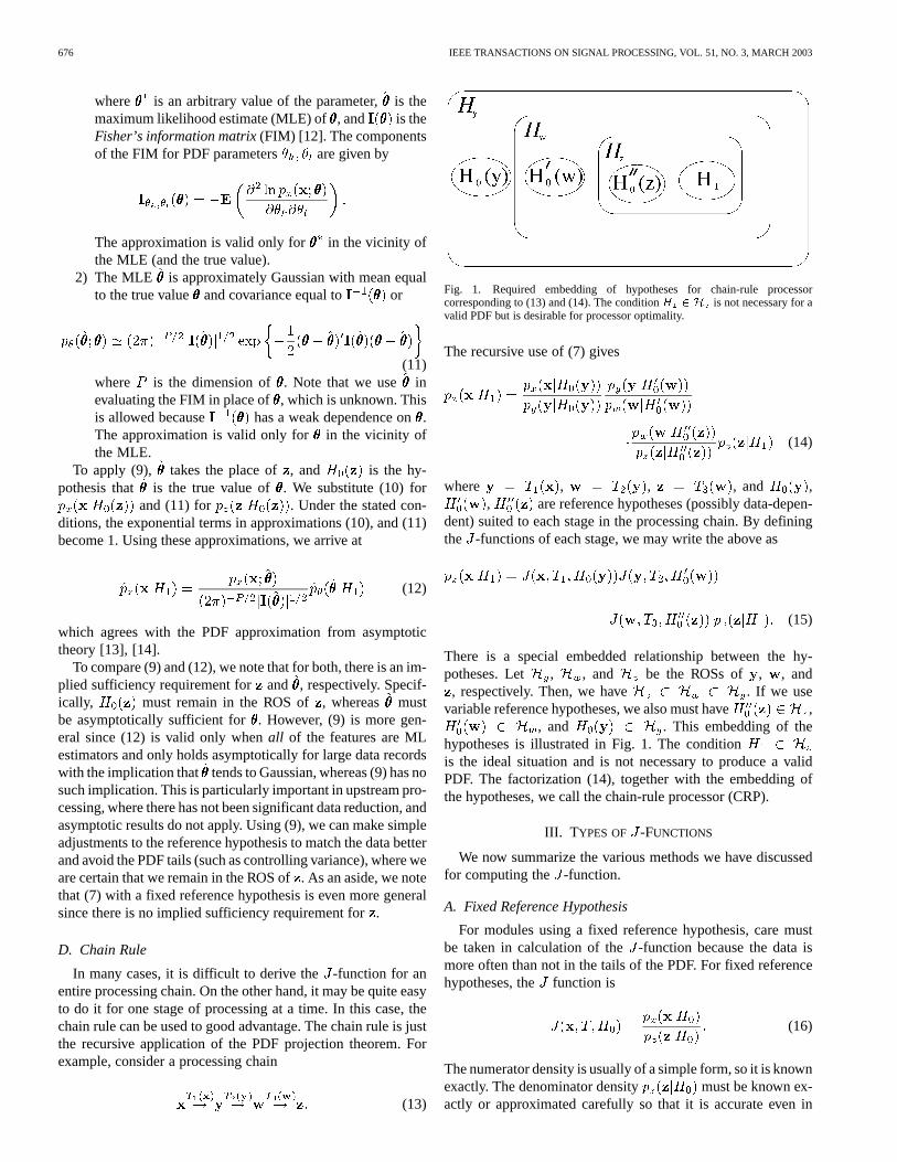
Fig. 1. Required embedding of hypotheses for chain-rule processorcorresponding to (13) and (14). The conditionH 2 H is not necessary for avalid PDF but is desirable for processor optimality.

The recursive use of (7) gives

(14)

where , , , and ,, are reference hypotheses (possibly data-depen-

dent) suited to each stage in the processing chain. By definingthe -functions of each stage, we may write the above as

(15)

There is a special embedded relationship between the hy-potheses. Let , , and be the ROSs of , , and, respectively. Then, we have . If we use

variable reference hypotheses, we also must have ,, and . This embedding of the

hypotheses is illustrated in Fig. 1. The conditionis the ideal situation and is not necessary to produce a validPDF. The factorization (14), together with the embedding ofthe hypotheses, we call the chain-rule processor (CRP).

III. T YPES OF -FUNCTIONS

We now summarize the various methods we have discussedfor computing the -function.

A. Fixed Reference Hypothesis

For modules using a fixed reference hypothesis, care mustbe taken in calculation of the-function because the data ismore often than not in the tails of the PDF. For fixed referencehypotheses, the function is

(16)

The numerator density is usually of a simple form, so it is knownexactly. The denominator density must be known ex-actly or approximated carefully so that it is accurate even in


the far tails of the PDF. The saddlepoint approximation (SPA),which was described in a recent publication [15], provides a so-lution for cases when the exact PDF cannot be derived but theexact moment-generating function (MGF) is known. The SPAis known to be accurate in the far tails of the PDF [15].

Example 2: As a very simple example of a fixed-referencemodule, let be a time-series, and letbe the power estimate

For being WGN, is quite simple to write, namely

(17)

Clearly, is a Chi-square RV with degrees of freedom scaledby . Thus

(18)

B. Variable Reference Hypothesis Modules

For a variable reference hypotheses, thefunction is

(19)

Modules using a variable reference are usually designed to po-sition the reference hypothesis at the peak of the denominatorPDF, which is approximated by the CLT.

Example 3: We can use the Example 2 and redesign themodule as a variable reference module. Now, instead of usingreference , we use the reference hypothesis thathas variance . Thus

(20)

Now, will still be Chi-square, but we can approximate its PDFby the CLT. Accordingly, has mean and variance

. Thus

(21)

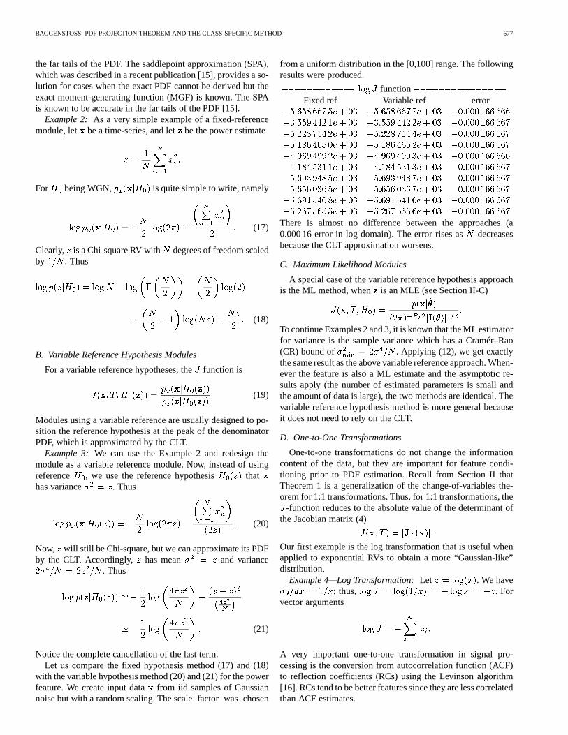
Notice the complete cancellation of the last term.Let us compare the fixed hypothesis method (17) and (18)

with the variable hypothesis method (20) and (21) for the powerfeature. We create input datafrom iid samples of Gaussiannoise but with a random scaling. The scale factor was chosen

from a uniform distribution in the [0,100] range. The followingresults were produced.

functionFixed ref Variable ref error

There is almost no difference between the approaches (a0.000 16 error in log domain). The error rises asdecreasesbecause the CLT approximation worsens.

C. Maximum Likelihood Modules

A special case of the variable reference hypothesis approachis the ML method, when is an MLE (see Section II-C)

To continue Examples 2 and 3, it is known that the ML estimatorfor variance is the sample variance which has a Cramér–Rao(CR) bound of . Applying (12), we get exactlythe same result as the above variable reference approach. When-ever the feature is also a ML estimate and the asymptotic re-sults apply (the number of estimated parameters is small andthe amount of data is large), the two methods are identical. Thevariable reference hypothesis method is more general becauseit does not need to rely on the CLT.

D. One-to-One Transformations

One-to-one transformations do not change the informationcontent of the data, but they are important for feature condi-tioning prior to PDF estimation. Recall from Section II thatTheorem 1 is a generalization of the change-of-variables the-orem for 1:1 transformations. Thus, for 1:1 transformations, the

-function reduces to the absolute value of the determinant ofthe Jacobian matrix (4)

Our first example is the log transformation that is useful whenapplied to exponential RVs to obtain a more “Gaussian-like”distribution.

Example 4—Log Transformation:Let . We have; thus, . For

vector arguments

A very important one-to-one transformation in signal pro-cessing is the conversion from autocorrelation function (ACF)to reflection coefficients (RCs) using the Levinson algorithm[16]. RCs tend to be better features since they are less correlatedthan ACF estimates.


Fig. 2. Block diagram of a class-specific classifier.

Example 5—Conversion From ACF to RCs:Let ,where and , where

are the RCs. The Jacobian is

Although the RCs are uncorrelated, they are subject to thelimit , which gives their distribution a discontinuity. Toobtain more Gaussian behavior, the log-bilinear transformationis recommended (thanks to S. Kay).

Example 6—Log Bilinear Transformation:Let

We have

Additionally, taking the log of the first feature () results ina further improvement.

IV. A PPLICATION OFTHEOREM 1 TO CLASSIFICATION

A. Classifier Architecture

Application of the PDF projection theorem to classificationis simply a matter of substituting (9) into (1). In other words,

we implement the classical Neyman–Pearson classifier but withthe class PDFs factored using the PDF projection theorem

at

(22)where we have allowed for class-dependent, data-dependent,reference hypotheses.

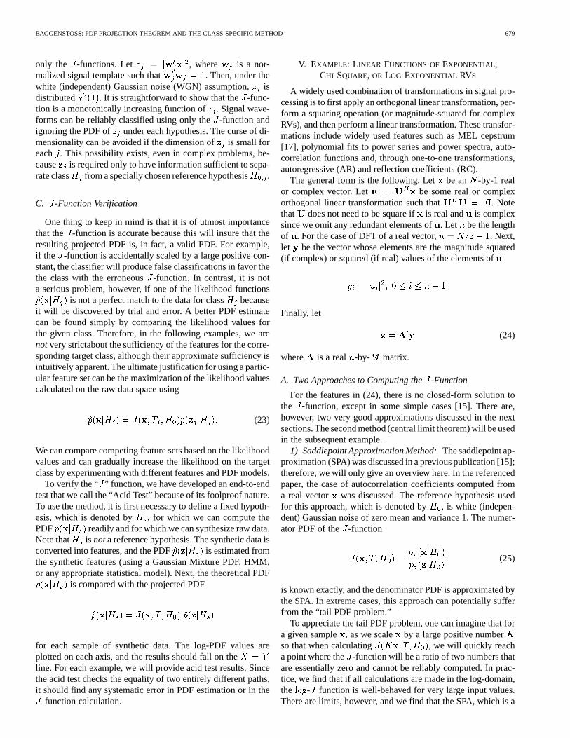
The chain-rule processor (14) is ideally suited to classifiermodularization. Fig. 2 is a block diagram of a class-specific clas-sifier. The packaging of the feature calculation together with the

-function calculation is called the class-specific module. Eacharm of the classifier is composed of a series of modules calleda “chain.”

B. Feature Selectivity: Classifying Without Training

The -function and the feature PDF provide a factorization ofthe raw data PDF into trained and untrained components. Theability of the -function to provide a “peak” at the “correct”feature set gives the classifier a measure of classification per-formance without needing to train. In fact, it is not uncommonthat the -function dominates, eliminating the need to train atall. This we call thefeature selectivity effect. For a fixed amountof raw data, as the dimension of the feature set decreases, indi-cating a larger rate of data compression, the effect of the-func-tion compared with the effect of the feature PDF increases. Anexample where the-function dominates is a bank of matchedfilter for known signals in noise. If we regard the matched filtersas feature extractors and the matched filter outputs as scalar fea-tures, it may be shown that this method is identical to comparing


only the -functions. Let , where is a nor-malized signal template such that . Then, under thewhite (independent) Gaussian noise (WGN) assumption,isdistributed . It is straightforward to show that the-func-tion is a monotonically increasing function of. Signal wave-forms can be reliably classified using only the-function andignoring the PDF of under each hypothesis. The curse of di-mensionality can be avoided if the dimension ofis small foreach . This possibility exists, even in complex problems, be-cause is required only to have information sufficient to sepa-rate class from a specially chosen reference hypothesis .

C. -Function Verification

One thing to keep in mind is that it is of utmost importancethat the -function is accurate because this will insure that theresulting projected PDF is, in fact, a valid PDF. For example,if the -function is accidentally scaled by a large positive con-stant, the classifier will produce false classifications in favor thethe class with the erroneous-function. In contrast, it is nota serious problem, however, if one of the likelihood functions

is not a perfect match to the data for classbecauseit will be discovered by trial and error. A better PDF estimatecan be found simply by comparing the likelihood values forthe given class. Therefore, in the following examples, we arenotvery strictabout the sufficiency of the features for the corre-sponding target class, although their approximate sufficiency isintuitively apparent. The ultimate justification for using a partic-ular feature set can be the maximization of the likelihood valuescalculated on the raw data space using

(23)

We can compare competing feature sets based on the likelihoodvalues and can gradually increase the likelihood on the targetclass by experimenting with different features and PDF models.

To verify the “ ” function, we have developed an end-to-endtest that we call the “Acid Test” because of its foolproof nature.To use the method, it is first necessary to define a fixed hypoth-esis, which is denoted by , for which we can compute thePDF readily and for which we can synthesize raw data.Note that is nota reference hypothesis. The synthetic data isconverted into features, and the PDF is estimated fromthe synthetic features (using a Gaussian Mixture PDF, HMM,or any appropriate statistical model). Next, the theoretical PDF

is compared with the projected PDF

for each sample of synthetic data. The log-PDF values areplotted on each axis, and the results should fall on theline. For each example, we will provide acid test results. Sincethe acid test checks the equality of two entirely different paths,it should find any systematic error in PDF estimation or in the

-function calculation.

V. EXAMPLE: LINEAR FUNCTIONS OFEXPONENTIAL,CHI-SQUARE, OR LOG-EXPONENTIAL RVS

A widely used combination of transformations in signal pro-cessing is to first apply an orthogonal linear transformation, per-form a squaring operation (or magnitude-squared for complexRVs), and then perform a linear transformation. These transfor-mations include widely used features such as MEL cepstrum[17], polynomial fits to power series and power spectra, auto-correlation functions and, through one-to-one transformations,autoregressive (AR) and reflection coefficients (RC).

The general form is the following. Let be an -by-1 realor complex vector. Let be some real or complexorthogonal linear transformation such that . Notethat does not need to be square ifis real and is complexsince we omit any redundant elements of. Let be the lengthof . For the case of DFT of a real vector, . Next,let be the vector whose elements are the magnitude squared(if complex) or squared (if real) values of the elements of

Finally, let

(24)

where is a real -by- matrix.

A. Two Approaches to Computing the-Function

For the features in (24), there is no closed-form solution tothe -function, except in some simple cases [15]. There are,however, two very good approximations discussed in the nextsections. The second method (central limit theorem) will be usedin the subsequent example.

1) Saddlepoint Approximation Method:The saddlepoint ap-proximation (SPA) was discussed in a previous publication [15];therefore, we will only give an overview here. In the referencedpaper, the case of autocorrelation coefficients computed froma real vector was discussed. The reference hypothesis usedfor this approach, which is denoted by , is white (indepen-dent) Gaussian noise of zero mean and variance 1. The numer-ator PDF of the -function

(25)

is known exactly, and the denominator PDF is approximated bythe SPA. In extreme cases, this approach can potentially sufferfrom the “tail PDF problem.”

To appreciate the tail PDF problem, one can imagine that fora given sample , as we scale by a large positive numberso that when calculating , we will quickly reacha point where the -function will be a ratio of two numbers thatare essentially zero and cannot be reliably computed. In prac-tice, we find that if all calculations are made in the log-domain,the - function is well-behaved for very large input values.There are limits, however, and we find that the SPA, which is a


recursive search for the saddlepoint itself, will eventually haveconvergence problems. To alleviate this problem, we use a vari-able reference hypothesis (see Section II-B). Letbe a roughestimate of the variance of. Let be the hypothesis that theinput variance equals. Assuming and are in the ROSof , (25) is theoretically independent of , and thus

However

where is the dimension of . Therefore

(26)

which provides a convenient way to normalizeprior to calcu-lating the SPA.

2) CLT Method: The second method that gives us a work-able solution is the CLT. We use the chain rule to separately an-alyze the two stages: a) orthogonal transformation and squaringand b) linear transformation. We will design a two-module chainfor a subset of the autocorrelation function (ACF) estimates. Theprocessing chain necessary to compute the ACF coefficients canbe broken down into two stages:

1) Compute , which are the magnitude-squared FFT bins.2) Compute , which is a subset of the elements of IFFT,

which is the real part of the inverse FFT of.

B. Structure of the Examples

As explained previously, a class-specific classifier can be or-ganized into “modules”. Each module consist of a feature trans-formation and a -function calculation. The -function requiresthe definition of a reference hypothesis and the calculation of thenumerator (input) and denominator (output) PDF. Accordingly,we organize this example and those that follow into modules.For each module, we explain the following.

1) Features and ROS. We describe the feature transforma-tion and the ROS for the features (see Sec-tion II-B). Ideally, the ROS, which is denoted by , in-cludes the “target class” for which this feature set isdesigned.

2) Reference Hypothesis. We define the reference hypoth-esis used in the -function. Often, this hypothesis isa data-dependent reference, which is written .

3) Input PDF . We define this as the numerator of thefunction.

4) Output PDF. This is the denominator of the-function.5) Test Results. When appropriate, we present results of the

“acid test” (Section IV-C).

C. Stage 1: DFT Magnitude-Squared

Stage 1 of the two-stage CLT approach is discussed here.

1) Features and Region of Sufficiency:Let be the lengthvector of magnitude-squared bins of the DFT of.

where

The ROS of is quite broad, encompassing all Gaussian pro-cesses with a power spectrum.

2) Reference Hypothesis:For our reference hypothesis forthis stage, we use , which is the standard normal density(WGN hypothesis with unit variance).

3) Input PDF: We have

(27)

4) Output PDF: Note that under , is a set of indepen-dent RVs. It is easily shown that , obey the densitywith mean and variance 2 . In addition, obeythe or exponential density with mean and variance .Thus

(28)

where

(29)and

(30)

and is the mean of the elements of( ).

D. Stage 2: Linear Transformation

Stage 2 of the two-stage CLT approach is discussed here. Instage 2, we apply a linear transformation to. We use ACF asan example, but the basic method applies to any linear transfor-mation.

1) Features and Region of Sufficiency:We let be the firstcircular ACF samples

(31)

where is taken modulo- . We use the circular ACF esti-mates in this example for simplicity because they may be writtenin terms of , but the -function may be found for any variety


of ACF estimate. The features (31) may be written in terms ofas follows:

(32)

This has a compact matrix notation

where is the ( )-by-( ) matrix defined by

(33)

(34)

Since is the ACF estimates of order, the approximate ROSis all AR processes of order and less.

2) Reference Hypothesis:Because we intend to use the CLTto approximate the -function denominator, we need to use avariable reference hypothesis such that the mean ofunder is equal to or close to itself. There are two pos-sible methods. For arbitrary matrices, this can be done byprojecting the input vector upon the column space of. Let

be the hypothesis that has mean

(35)

Notice that , that is, under , the mean of isitself.

One possible problem that can occur is if in (35) happensto be negative, which is quite possible, but not allowed. A suit-able solution is to use a constrained optimization, that is, choose

such that it is positive, and is as close as possible to.A more satisfying way to guarantee a positivein the case

of ACF is the following. We let be the hypothesis thatobeys the AR spectrum corresponding to. Thus, we must usethe Levinson algorithm to solve for theth-order AR coeffi-cients , . If is the DFT of (padded to length ), then

is the AR spectrum corresponding to. We let

(36)

For large , we have .3) Input PDF: We need to evaluate and

. We assume { } are a set of independent expo-

nential and RVs with means corresponding to {}, whichare the elements of . Specifically

(37)

and

(38)

4) Output PDF: Because is “close” to , we approx-imate by the central limit theorem (CLT). Under

, the elements of are independent with mean and di-agonal covariance , which are defined by

.

We can then easily compute the mean and covariance of:

and

det

det

(39)

where in the last step, we make the approximation .This approximation becomes better asbecomes larger. Notealso that the method just described is closely related to the MLapproach. In fact, is related to the Fisher’s information ofthe ACF estimates [16].

E. Test Results

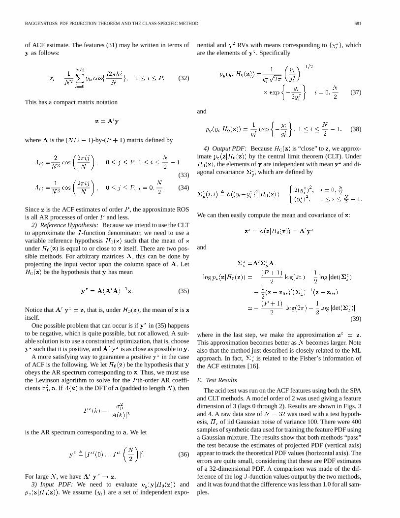
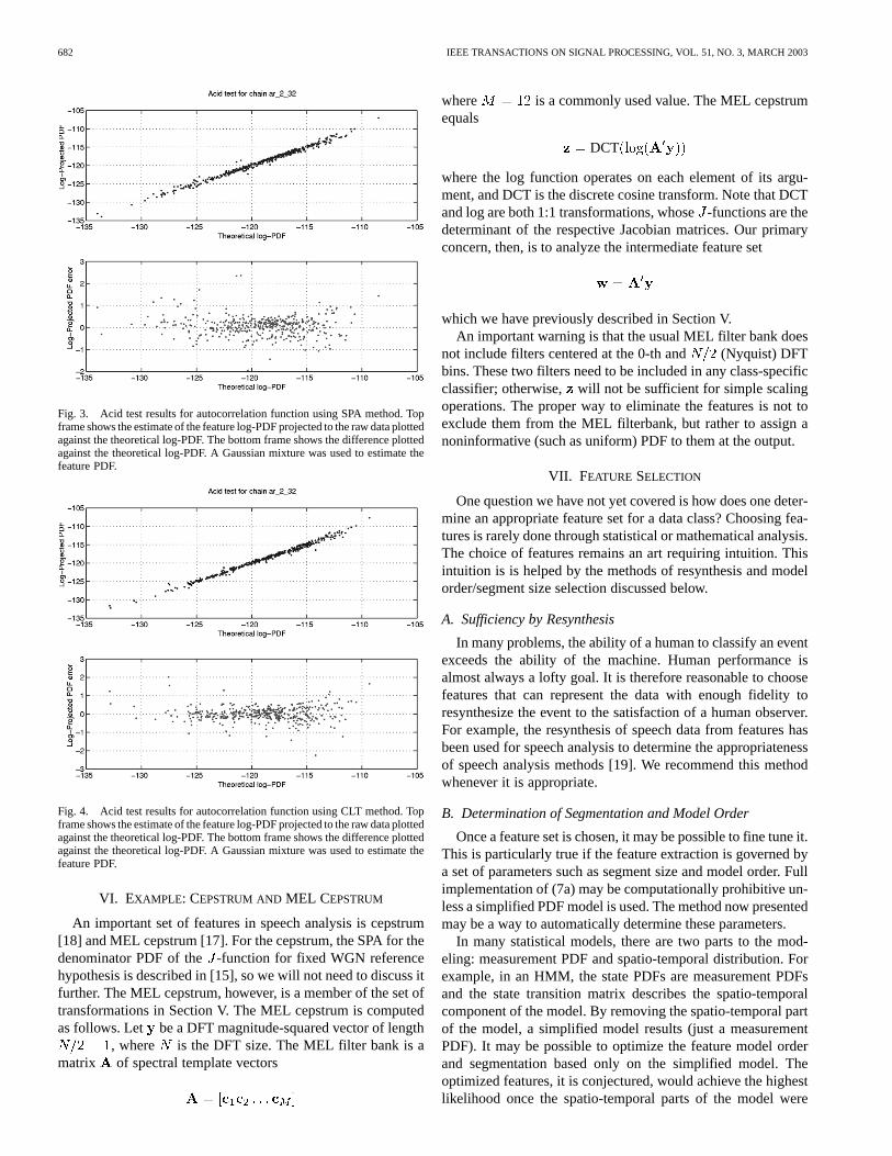
The acid test was run on the ACF features using both the SPAand CLT methods. A model order of 2 was used giving a featuredimension of 3 (lags 0 through 2). Results are shown in Figs. 3and 4. A raw data size of was used with a test hypoth-esis, of iid Gaussian noise of variance 100. There were 400samples of synthetic data used for training the feature PDF usinga Gaussian mixture. The results show that both methods “pass”the test because the estimates of projected PDF (vertical axis)appear to track the theoretical PDF values (horizontal axis). Theerrors are quite small, considering that these are PDF estimatesof a 32-dimensional PDF. A comparison was made of the dif-ference of the log -function values output by the two methods,and it was found that the difference was less than 1.0 for all sam-ples.


Fig. 3. Acid test results for autocorrelation function using SPA method. Topframe shows the estimate of the feature log-PDF projected to the raw data plottedagainst the theoretical log-PDF. The bottom frame shows the difference plottedagainst the theoretical log-PDF. A Gaussian mixture was used to estimate thefeature PDF.

Fig. 4. Acid test results for autocorrelation function using CLT method. Topframe shows the estimate of the feature log-PDF projected to the raw data plottedagainst the theoretical log-PDF. The bottom frame shows the difference plottedagainst the theoretical log-PDF. A Gaussian mixture was used to estimate thefeature PDF.

VI. EXAMPLE: CEPSTRUM ANDMEL CEPSTRUM

An important set of features in speech analysis is cepstrum[18] and MEL cepstrum [17]. For the cepstrum, the SPA for thedenominator PDF of the -function for fixed WGN referencehypothesis is described in [15], so we will not need to discuss itfurther. The MEL cepstrum, however, is a member of the set oftransformations in Section V. The MEL cepstrum is computedas follows. Let be a DFT magnitude-squared vector of length

, where is the DFT size. The MEL filter bank is amatrix of spectral template vectors

where is a commonly used value. The MEL cepstrumequals

DCT

where the log function operates on each element of its argu-ment, and DCT is the discrete cosine transform. Note that DCTand log are both 1:1 transformations, whose-functions are thedeterminant of the respective Jacobian matrices. Our primaryconcern, then, is to analyze the intermediate feature set

which we have previously described in Section V.An important warning is that the usual MEL filter bank does

not include filters centered at the 0-th and (Nyquist) DFTbins. These two filters need to be included in any class-specificclassifier; otherwise, will not be sufficient for simple scalingoperations. The proper way to eliminate the features is not toexclude them from the MEL filterbank, but rather to assign anoninformative (such as uniform) PDF to them at the output.

VII. FEATURE SELECTION

One question we have not yet covered is how does one deter-mine an appropriate feature set for a data class? Choosing fea-tures is rarely done through statistical or mathematical analysis.The choice of features remains an art requiring intuition. Thisintuition is is helped by the methods of resynthesis and modelorder/segment size selection discussed below.

A. Sufficiency by Resynthesis

In many problems, the ability of a human to classify an eventexceeds the ability of the machine. Human performance isalmost always a lofty goal. It is therefore reasonable to choosefeatures that can represent the data with enough fidelity toresynthesize the event to the satisfaction of a human observer.For example, the resynthesis of speech data from features hasbeen used for speech analysis to determine the appropriatenessof speech analysis methods [19]. We recommend this methodwhenever it is appropriate.

B. Determination of Segmentation and Model Order

Once a feature set is chosen, it may be possible to fine tune it.This is particularly true if the feature extraction is governed bya set of parameters such as segment size and model order. Fullimplementation of (7a) may be computationally prohibitive un-less a simplified PDF model is used. The method now presentedmay be a way to automatically determine these parameters.

In many statistical models, there are two parts to the mod-eling: measurement PDF and spatio-temporal distribution. Forexample, in an HMM, the state PDFs are measurement PDFsand the state transition matrix describes the spatio-temporalcomponent of the model. By removing the spatio-temporal partof the model, a simplified model results (just a measurementPDF). It may be possible to optimize the feature model orderand segmentation based only on the simplified model. Theoptimized features, it is conjectured, would achieve the highestlikelihood once the spatio-temporal parts of the model were


restored. We have conducted many experiments that supportthis conjecture.

The particulars of the method are now presented. Let the fea-ture data be written , where is a par-ticular choice of segment size and/or model order andisthe corresponding total number of observation vectors corre-sponding to choice. Note that we have collected all the avail-able data from all events into one mass, forgetting the temporalor spatial organization, and forgetting which event the obser-vations are from. We also assume that are low enough indimension that a parametric PDF estimator (i.e., Gaussian mix-ture) can be estimated from the data. Let the data be divided intoa training set ( , ) and testing set ( , ) for cross-val-idation. Next, we estimate the PDF

using for model choice . The feature PDF is projected tothe input data space where it can be compared across differentvalues of . We have

where is the aggregate - -function for the dataset. Next, is calculated for ( , ). For added accuracy,

can also be computed by swapping and and aver-aging. The optimal choice of is that which maximizes .

This approach is robust against overparameterization becauseas the model order (and dimension of) increases above theoptimal value, the ability to estimate the PDF worsens and theaverage of the cross-validated likelihood will begin to fall.

C. Example

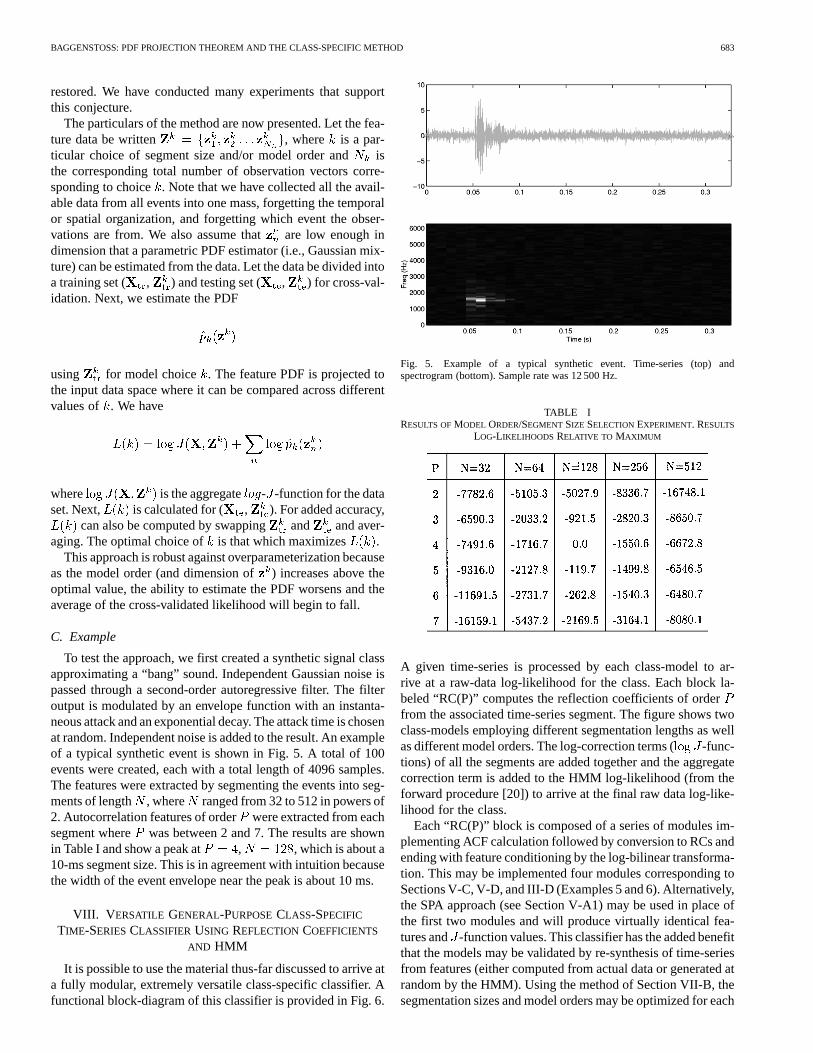
To test the approach, we first created a synthetic signal classapproximating a “bang” sound. Independent Gaussian noise ispassed through a second-order autoregressive filter. The filteroutput is modulated by an envelope function with an instanta-neous attack and an exponential decay. The attack time is chosenat random. Independent noise is added to the result. An exampleof a typical synthetic event is shown in Fig. 5. A total of 100events were created, each with a total length of 4096 samples.The features were extracted by segmenting the events into seg-ments of length , where ranged from 32 to 512 in powers of2. Autocorrelation features of orderwere extracted from eachsegment where was between 2 and 7. The results are shownin Table I and show a peak at , , which is about a10-ms segment size. This is in agreement with intuition becausethe width of the event envelope near the peak is about 10 ms.

VIII. V ERSATILE GENERAL-PURPOSECLASS-SPECIFIC

TIME-SERIESCLASSIFIER USING REFLECTION COEFFICIENTS

AND HMM

It is possible to use the material thus-far discussed to arrive ata fully modular, extremely versatile class-specific classifier. Afunctional block-diagram of this classifier is provided in Fig. 6.

Fig. 5. Example of a typical synthetic event. Time-series (top) andspectrogram (bottom). Sample rate was 12 500 Hz.

TABLE IRESULTS OFMODEL ORDER/SEGMENT SIZE SELECTION EXPERIMENT. RESULTS

LOG-LIKELIHOODS RELATIVE TO MAXIMUM

A given time-series is processed by each class-model to ar-rive at a raw-data log-likelihood for the class. Each block la-beled “RC(P)” computes the reflection coefficients of orderfrom the associated time-series segment. The figure shows twoclass-models employing different segmentation lengths as wellas different model orders. The log-correction terms ( -func-tions) of all the segments are added together and the aggregatecorrection term is added to the HMM log-likelihood (from theforward procedure [20]) to arrive at the final raw data log-like-lihood for the class.

Each “RC(P)” block is composed of a series of modules im-plementing ACF calculation followed by conversion to RCs andending with feature conditioning by the log-bilinear transforma-tion. This may be implemented four modules corresponding toSections V-C, V-D, and III-D (Examples 5 and 6). Alternatively,the SPA approach (see Section V-A1) may be used in place ofthe first two modules and will produce virtually identical fea-tures and -function values. This classifier has the added benefitthat the models may be validated by re-synthesis of time-seriesfrom features (either computed from actual data or generated atrandom by the HMM). Using the method of Section VII-B, thesegmentation sizes and model orders may be optimized for each


Fig. 6. Block diagram of an HMM and RC-based class-specific classifier. A given time-series is processed by each class-model to arrive at a raw-datalog-likelihood for the class. Each block labeled “RC(P)” computes theP th order reflection coefficients from the corresponding time-series segment and isimplemented by a series of modules.

class individually, eliminating the need to “compromise,” and,because it is a class-specific classifier, features of any kind maybe used. Adding new class processors will not affect the existingclass processors or their training.

IX. CONCLUSIONS

We have introduced a powerful new theorem that opens up awide range of new statistical methods for signal processing, pa-rameter estimation, and hypothesis testing. Instead of needing acommon feature space for likelihood comparisons, the theoremallows likelihood comparisons to be made on a common rawdata space, while the difficult problem of PDF estimation canbe accomplished in separate feature spaces. We have discussedthe recursive application of the theorem which gives a hierar-chical breakdown and allows processing streams to be analyzedin stages. Whereas previous publications on the method haverelied on a common fixed reference hypothesis, this paper haspresented the use of class-dependent and data-dependent refer-ence hypotheses and has explored the relationship to asymptoticmaximum likelihood theory. The use of a data-dependent refer-ence hypothesis allows two new methods of analyzing the fea-ture sets – maximum likelihood (ML) and central limit theorem(CLT). These extensions significantly broaden the applicabilityof the method. We have illustrated the use of the approach usingcommon feature types including autoregressive and MEL cep-strum features. We have also presented a method of combinedfeature/model order selection that is enabled by the class-spe-cific approach. Finally, we have provided an example of a ver-satile class-specific classifier using autoregressive features.

REFERENCES

[1] P. Baggenstoss, “Class-specific features in classification,”IEEE Trans.Signal Processing, vol. 47, pp. 3428–3432, Dec. 1999.

[2] S. M. Kay, “Sufficiency, classification and the class-specific feature the-orem,” IEEE Trans. Inform Theory, vol. 46, pp. 1654–1658, July 2000.

[3] Frimpong-Ansah, K. Pearce, D. Holmes, and W. Dixon, “A sto-chastic/feature based recognizer and its training algorithm,” inProc.ICASSP, vol. 1, 1989, pp. 401–404.

[4] S. Kumar, J. Ghosh, and M. Crawford, “A versatile framework for la-beling imagery with large number of classes,” inProc. Int. Joint Conf.Neural Networks, Washington, DC, 1999, pp. 2829–2833.

[5] , “A hierarchical multiclassifier system for hyperspectral data anal-ysis,” in Multiple Classifier Systems, J. Kittler and F. Roli, Eds. NewYork: Springer, 2000, pp. 270–279.

[6] H. Watanabe, T. Yamaguchi, and S. Katagiri, “Discriminative metric de-sign for robust pattern recognition,”IEEE Trans. Signal Processing, vol.45, pp. 2655–2661, Nov. 1997.

[7] P. Belhumeur, J. Hespanha, and D. Kriegman, “Eigenfaces vs. Fisher-faces: Recognition using class specific linear projection,”IEEE Trans.Pattern Anal. Machine Intell., vol. 19, pp. 711–720, July 1997.

[8] D. Sebald, “Support vector machines and the multiple hypothesis testproblem,”IEEE Trans. Signal Processing, vol. 49, pp. 2865–2872, Nov.2001.

[9] I.-S. Oh, J.-S. Lee, and C. Y. Suen, “A class-modularity for characterrecognition,” inProc. Int. Conf. Document Anal. Recognition, Seattle,WA, Sept. 2001, pp. 64–68.

[10] E. Sali and S. Ullman, “Combining class-specific fragments for objectclassification,” in Proc. British Machine Vision Conf., 1999, pp.203–213.

[11] P. M. Baggenstoss, “A modified Baum-Welch algorithm for hiddenMarkov models with multiple observation spaces,”IEEE Trans. SpeechAudio Processing, vol. 9, pp. 411–416, May 2001.

[12] D. R. Cox and D. V. Hinkley,Theoretical Statistics. London, U.K.:Chapman and Hall, 1974.

[13] R. L. Strawderman, “Higher-order asymptotic approximation: Laplace,saddlepoint, and related methods,”J. Amer. Statist. Assoc., vol. 95, pp.1358–1364, Dec. 2000.


[14] J. Durbin, “Approximations for densities of sufficient estimators,”Biometrika, vol. 67, no. 2, pp. 311–333, 1980.

[15] S. M. Kay, A. H. Nuttall, and P. M. Baggenstoss, “Multidimensionalprobability density function approximation for detection, classificationand model order selection,”IEEE Trans. Signal Processing, pp.2240–2252, Oct. 2001.

[16] S. Kay, “Modern spectral estimation,” inTheory and Applica-tions. Englewood Cliffs, NJ: Prentice-Hall, 1998.

[17] J. W. Picone, “Signal modeling techniques in speech recognition,”Proc.IEEE, vol. 81, pp. 1215–1247, Sept. 1993.

[18] A. Oppenheim and R. Schafer, “Homomorphic analysis of speech,”IEEE Trans. Audio Electroacoust., vol. AU-16, pp. 221–226, 1968.

[19] C. Bell, H. Fujisaki, J. Heinz, K. Stevens, and A. House, “Reductionof speech spectra by analysis-by-synthesis techniques,”J. Acoust. Soc.Amer., pp. 1725–1736, Dec. 1961.

[20] L. R. Rabiner, “A tutorial on hidden Markov models and selected appli-cations in speech recognition,”Proc. IEEE, vol. 77, pp. 257–286, Feb.1989.

Paul M. Baggenstoss(M’90) received the Ph.D. de-gree in electrical engineering (statistical signal pro-cessing) from the University of Rhode Island (URI),Kingston, in 1990.

Since then, he has been applying signal processingand hypothesis testing (classification) to sonarproblems. From 1979 to 1996, he was with RaytheonCo, Portsmouth, RI. Since 1996, he has been with theNaval Undersea Warfare Center (NUWC), Newport,RI. He is the author of numerous conference andjournal papers in the field of signal processing and

classification and has taught part-time as an adjunct professor of electricalengineering at the University of Connecticut, Storrs.

Dr. Baggenstoss received the 2002 URI Excellence Award in Science andTechnology.

672 ieee transactions on signal processing, vol. 51, …krim. the author is with the naval undersea...

Documents