CHAPTER 5

MULTIPLE SCALES

5.1. OVERVIEW OF MULTIPLE SCALES AND AVERAGING

This chapter and the next concern initial value problems of oscillatory typeon long intervals of time. Until Section 5.4, we will study autonomousoscillatory second order initial value problems of the form

Y + kly =v(0) _ «, (5.1.1)

v(o) =P.

In Section 5.4 it will be shown that this and many other systems, includingperiodically forced oscillators and systems of several coupled oscillators,can be put into periodic standard form

u = ef(u,t,e), (5.1.2)

where u = (u1, ... ,UN) is an N-dimensional vector variable and f is peri-odic in t. Because of its generality and simplicity, periodic standard formwill be used in the rest of this chapter and most of the next. It may appearthat changing an equation into standard form is an unnecessary step re-quiring extra work, but in fact the variables which form the components ofu are often exactly those of greatest interest from the standpoint of applica-tions. In addition, theoretical discussions can be given once for equationsin standard form and then applied to a wide variety of problems, Bach ofwhich would require separate treatment if standard form were not used.

227

Dow

nloa

ded

02/1

1/16

to 1

28.6

1.77

.45.

Red

istr

ibut

ion

subj

ect t

o SI

AM

lice

nse

or c

opyr

ight

; see

http

://w

ww

.sia

m.o

rg/jo

urna

ls/o

jsa.

php

228 MULTIPLE SCALES

For these reasons we consider standard form to be an advantage ratherthan a disadvantage. On the other hand, beginning with (5.1.1) makes fora smooth transition from previous chapters.

Of course, equation (5.1.1) has been studied in Section 4.4 by the Lind-stedt method. However, due to the inherent limitations of that method,only periodic solutions could be found at that time. For instance, the limitcycle of a Van der Pol equation could be located, but it was not possibleto find approximations of the nonperiodic orbits that approach the limitcycle. It is the purpose of the method of multiple scales and the method ofaveraging to remove this limitation. These methods enable the construc-tion of an approximate solution with arbitrary initial conditions which nolonger need to satisfy a determining equation. One feature of the Lindstedtmethod carries over to these new methods: the results are usually valid onan "expanding interval" of time. In most cases this expanding interval haslength 0(1 /c). Error estimates on longer intervals, such as 0(1 /e 2 ) or evenfor all time, can be obtained under various special circumstances, but thereare no general results of this type. In particular, the "trade-off" propertyof Lindstedt expansions expressed in equation (4.2.15) is definitely falsefor multiple scale and averaging methods in general.

The solution of the reduced problem of (5.1.1) can be written in severalways, such as

y=Acoskt+Bsinkt ( 5.1.3)

and

y = p cos(>p — kt), (5.1.4)

where A, B, p, and yr are constants of integration. The first of these, (5.1.3),will be called Cartesian form, and (5.1.4) will be called polar form, becausethe relations A = p cos yr and B = p sin v, which follow from (5.1.3)and (5.1.4), are the same as the relations between Cartesian and polarcoordinates in the plane. (This will become more explicit in Section 5.4and explains our preference for (5.1.4) over forms such as y = asin(6 +kt).) The solution of the reduced problem can be regarded as the "zeroth"approximation to the solution of the perturbed problem (5.1.1). Accordingto the results of Chapter 2, this zeroth approximation has an error 0(e)uniformly for t in a finite interval 0 < t < T, and is (in most cases) uselesson longer intervals. The first task of both the method of multiple scalesand the method of averaging is to improve this zeroth approximation toproduce a "first approximation" having error 0(e) uniformly for t in anexpanding interval of the foren 0 < t < L/e. This is an essentially differentproblem from that of improving the accuracy to 0(e2 ) on a finite interval,a task which is accomplished quite satisfactorily by regular perturbationtheory.

Dow

nloa

ded

02/1

1/16

to 1

28.6

1.77

.45.

Red

istr

ibut

ion

subj

ect t

o SI

AM

lice

nse

or c

opyr

ight

; see

http

://w

ww

.sia

m.o

rg/jo

urna

ls/o

jsa.

php

5.1. OVERVIEW OF MULTIPLE SCALES AND AVERAGING 229

The terms "zeroth" and "first" approximation, used in the last para-graph, have a slightly different significance here than in previous chapters.The phrase zeroth approximation always refers to the solution of the re-duced problem. In earlier chapters, the solution of the reduced problemwas also the leading term in the asymptotic series being constructed. How-ever, in the methode of multiple scales and averaging, the leading term ofthe asymptotic solution is not the solution of the reduced problem, but isalready an improvement over that solution. The phrase first approximationwill always be used to refer to the first improvement of the zeroth approx-imation. Therefore, in regular perturbation theory, the "first approxima-tion" consists of two terms of the asymptotic solution (the zeroth and firstorder terms, as measured by powers of e); in Chapters 5 and 6, the "firstapproximation" will consist only of the leading term of the asymptoticseries.

The method of multiple scales and the method of averaging both givethe same answer to the problem of finding a first approximation to the so-lution of (5.1.1) on an expanding interval, although they obtain this answerby quite different reasoning. The first approximation given by both meth-ods takes the same form as the zeroth approximation (5.1.3) or (5.1.4),except that the quantities A, B, p, and +p, which were constants of in-tegration, become slowly varying functions of time. More precisely, theapproximations take the form

y _ A(et) cos kt + B(et) sin kt (5.1.5)

or

y ^' p(et) cos(yr(et) — kt), (5.1.6)

where the functions of et are the solutions of certain differential equationswhich will be given in the next section. Any function of et can be consid-ered as a slowly varying function of time, since the derivative of such afunction contains a factor of e due to the chain rule. (Another way to lookat this is that t must increase a great deal before et will change very much,when e is small.) It is customary to write either T := et, or else To = t andT1 = et, so that the approximations take the form

y - A(r) cos kt + B(T) sin kt = A(T1) cos kTo + B(TI ) sin kTo(5.1.7)

or

y L2 p(z) cos(w(T) — kt) = p(T1) cos(w(Ti) — kTo). (5.1.8)

Here r is called slow time, and the variables t and r (or To and T1 ) arereferred to as two time scales. When form (5.1.8) is used, one speaks of

Dow

nloa

ded

02/1

1/16

to 1

28.6

1.77

.45.

Red

istr

ibut

ion

subj

ect t

o SI

AM

lice

nse

or c

opyr

ight

; see

http

://w

ww

.sia

m.o

rg/jo

urna

ls/o

jsa.

php

230 MULTIPLE SCALES

the method of slowly varying amplitude and phase, since p and yr are theamplitude and phase of the simple harmonic motion (5.1.4) in the reducedcase. (The "method" of slowly varying amplitude and phase is not actuallya method in itself, but only a notation which can be used with severalmethods such as averaging and multiple scales.)

In most applications of the methods of multiple scales or averaging,the first approximation is sufficient. Therefore this approximation will bediscussed at length, in both this chapter (Section 5.2) and the next (Sec-tions 6.1, 6.2, and 6.3). To go beyond the first approximation can be quitedifficult. Beyond the first approximation, the methods of averaging and ofmultiple scales do not always give the same results; in fact, each of thesemethods (multiple scales and averaging) has several forms, and these dif-ferent forms do not give the same results beyond the first approximation.(This is possible because these are generalized asymptotic expansions anddo not satisfy a uniqueness theorem like Theorem 1.8.3. The differentresults do not conflict with each other; each is a legitimate asymptotic ap-proximation of the exact solution.) The various multiple scale methodshave the reputation of being computationally simpler than the method ofaveraging after the first approximation, and this is no doubt true in manyspecific problems. On the other hand, the theoretical foundations of themethod of averaging are much better understood than those of multiplescales, and it is possible to draw many conclusions about the behavior ofthe solutions, such as stability and periodicity, from the averaging calcu-lations.

Higher order multiple scale methods for oscillatory problems can begrouped into three types:

1. Two-scale methods using To := t and Ti = T := et. The solutions arewritten in the form yo (t, r) + ey i (t, z) +

2. Two-scale methods using a strained time t+ :_ (vo +evl + e2 v2 + • • +

el vl ) t and a slow time T := et, with a suitable choice of v1 ,. . . , ve .The solutions appear as yo(t+, T) + eyl (t+, t) + • • • .

3. Multiple scale methods using M scales Tm := em t for m = 1, ... , M.The solutions are written yo(To, T1 ,. .. , TM) + eyl (To, T1 ,..., Tm) +• • • . A variation of this method (the "short form") omits one timescale in each successive term; for instante, a three-scale three-termsolution would look like yo(To, T1 , T2) + eyl(To, T1) + e2y2(To).

The theory of higher order approximations by the first of these meth-ods is fairly well understood. This form is applicable to a wide variety ofproblems and gives approximations to any order of accuracy which arevalid on expanding intervals of length 0(1 /E) but not (except under spe-cial circumstances) on longer intervals. The second and third forms areless satisfactory; they are intended to give approximations on expandingintervals longer than 0(1 /e), but they do not always work (even formally),D

ownl

oade

d 02

/11/

16 to

128

.61.

77.4

5. R

edis

trib

utio

n su

bjec

t to

SIA

M li

cens

e or

cop

yrig

ht; s

ee h

ttp://

ww

w.s

iam

.org

/jour

nals

/ojs

a.ph

p

5.1. OVERVIEW OF MULTIPLE SCALES AND AVERAGING 231

and why. The second form is motivated by the Lindstedt method; the ideais that many nonperiodic solutions have the form of damped oscillations---- ----in which the "periodic part" can be described using t+ -and the dampingtakes place on the time scale T. The third form is the most general, sinceit includes the first two, the first by taking M = 1, and the second sincet+ (taken to 9 terms) can be written as a function of the scales T0,..., Ti .In Section 5.3 (which may be omitted without loss of continuity) the firstand third of these methods will be illustrated.

To conclude this introductory section we will study a certain linear prob-lem of the form (5.1.1) "in reverse." That is, we will write down the ex-act solution, and then expand this solution into three different forms ofmultiple scale approximations and examine the error. This is, of course,"cheating," and is intended only to give insight; we are not actually usingthe method of multiple scales. (It is rather like "cheating" by using thequadratic formula in Chapter 1.) The example to be studied is

5'+2e5' +(1 +e)y=0,

y(0) = a, (5.1.9)y(0)=O,

with exact solution

y = ae-e 1 cos 1 + e — e2 t + Ea e -el sin 1 + E — e2 t. (5.1.10)1 +e —E

There are two effects apparent here: The damping term in (5.1.9) causesan exponential decay of the solution "on the time scale et," while bothperturbation terms interact to produce a frequency shift from the freefrequency 1. The shifted frequency can be expanded as

1 +E-E2 1 +ZE- 8E2 +48N E 3 +.... (5.1.11)

The first form of multiple scale solution which will be developed isa two-time-scale expansion using t and i. The technique for converting(5.1.10) into a two-time expansion is the same as that used in Section 4.7for changing a Lindstedt expansion into a two-time expansion. First, using(5.1.10) and (5.1.11), and the time scales t and r, write

y= ae-Tcos(t+ 8er+••.)

+Eae1 +e -E \

- T sin (t + 1 j + • • . . ( 5.1.12)

Next, expand each term in e holding t and T constant as though T were

Dow

nloa

ded

02/1

1/16

to 1

28.6

1.77

.45.

Red

istr

ibut

ion

subj

ect t

o SI

AM

lice

nse

or c

opyr

ight

; see

http

://w

ww

.sia

m.o

rg/jo

urna

ls/o

jsa.

php

232 MULTIPLE SCALES

an independent variable rather than a function of e. The result, throughorder e, is

^=' ae-= cos (t + 2T) + eae-1 5 z 11 sin (t + 1 T)y . (5.1.13)

The same argument as in Section 4.7 shows that the error committed inpassing from (5.1.10) to (5.1.13) is of order e 2 on expanding intervals oforder 1/e.

In fact, it is not hard to show that for this example the error is actually oforder e2 for all t > 0. Consider the first term of (5.1.12). When this term isexpanded in e and two terms are retained, the error committed is boundedby a constant times e2 te —". This expression reaches a maximum of e2e —`at t = 1, and since this maximum is less than e 2 , the error is of order e2as claimed. A similar analysis can be done for the second term of (5.1.12).The reason that a solution using only two time scales is able to remain validfor all time, rather than only on an expanding interval of order 1 /e, is thatthe exponential damping acts to reduce not only the size of the solution butalso of the error as t — ► oo. The mechanism is similar to that by which theregular perturbation solution of a damped oscillation was found to be validfor all time in Chapter 4, the difference being that in Chapter 4 the dampingwas of order 0(1) and here it is O(e); such damping is too wenk to rescuethe regular expansion from the ravages of its secular terras.

The second type of multiple scale approximation to be derived from(5.1.10) is a two-scale approximation using the scales

t+_ - 8e2) ,

\\

(5.1.14)

T=et.

Such an approximation can be obtained from (5.1.12) by dropping thedotted terms inside the trig functions:

y ae- t cos (t+ + 2 ) + eae-T sin (t+ + Z) . (5.1.15)

The final type of multiple scale expansion to be derived from (5.1.10)is a three-scale solution using t, T, and a := e2 t (or To, T1 , and T2). Weleave it to the reader (Exercise 5.1.1) to check that the complete two-term,three-scale expansion of (5.1.10) is

y^'ae-i cos (t+2T -5 a)

+eae-T ^1 - 4s a sin (t+ 2T- 5a . (5.1.16)

Dow

nloa

ded

02/1

1/16

to 1

28.6

1.77

.45.

Red

istr

ibut

ion

subj

ect t

o SI

AM

lice

nse

or c

opyr

ight

; see

http

://w

ww

.sia

m.o

rg/jo

urna

ls/o

jsa.

php

5.2. THE FIRST ORDER TWO-SCALE APPROXIMATION 233

The "short form" of this three-scale expansion is obtained by dropping afrom the term of order e; this is equivalent to (5.1.15). We have said thatadding a third time scale is usually an attempt to gain validity on a longertime interval. Here it is not needed for that purpose, since as noted above,(5.1.13) is already uniformly valid for all time because of the damping.

Exercises 5.1

1. Introduce t, r, and a as "independent" variables in (5.1.10) and expandin e to obtain (5.1.16).

5.2. THE FIRST ORDER TWO-SCALE APPROXIMATION

The idea of the two-scale method is to seek an approximate solution ofthe initial value problem

p + k2y =

y(0) = a, (5.2.1)(0)=fl

in the form

y Nyo(t, r) +ey,(t,T)+e2y2(t,T)+••• , (5.2.2)

where T = et. In this section, only the first term of (5.2.2) will be deter-mined. (Recall from the last section that yo is called the first approxima-tion, rather than the zeroth, because it is not equal to the solution of thereduced problem.) As in the Lindstedt method, finding yo requires that theequation for y, be written down as well; the equation for Y2 will also befound, since it is needed in the next section.

It must be understood that (5.2.2) is a rather peculiar way to write thesolution of an ordinary differential equation. There are actually only twoindependent variables, t and e, in (5.2.2); T is a function of these two,and so is not independent. Nevertheless, the principal steps in finding thecoefficients y„ are carried out as though t, z, and e were independent vari-ables. This is one reason why these steps cannot be justified rigorouslyin advance, but are merely heuristic. Secondly, it must be remarked that(5.2.2) is a generalized asymptotic expansion, since e enters both throughthe gauges (which are just the powers of e) and also through the coefficientsy„ by way of T. Although there is no general theorem allowing the differ-entiation of a generalized asymptotic expansion term by term (see Section1.8), it is nevertheless reasonable to construct the coefficients of (5.2.2) onthe assumption that such differentiation is possible, and then to justify theresulting series by direct error estimation afterwards. The procedure is totake the total derivative of (5.2.2) with respect to t twice, termwise, andsubstitute the result into (5.2.1). At the time of taking these derivatives, T

is regarded as equal to et, but afterwards, T is treated as an independent

Dow

nloa

ded

02/1

1/16

to 1

28.6

1.77

.45.

Red

istr

ibut

ion

subj

ect t

o SI

AM

lice

nse

or c

opyr

ight

; see

http

://w

ww

.sia

m.o

rg/jo

urna

ls/o

jsa.

php

(5.2.3)

(5.2.4)

(5.2.6a)

234 MULTIPLE SCALES

variable. Since the total dependence of each term Yn(t, f) upon t is a com­bination of its explicit dependence on t and its indirect dependence on tby way of r, the first and second total derivatives of each term are givenby the following formulas based on the chain rule:

d d 8 8dtYn(t, f) = d?n(t, et) = 8tYn(t, et) + e8fYn(t, f)

=Ynt(t, f) + eYnT(t, f),

d2dt 2Yn(t, f) =Ynu(t, f) + 2eYntT(t, f) + e2YnTT(t, f).

These equations are easiest to remember in operator form:

d 8 8dt = 8t +e 8 f ,

d2 8 2 8 2 8 2

dt2 = 8t2 + 2e8f8t + e2

8f2·

Substituting the derivatives of (5.2.2), computed in this way, into (5.2.1)gives the following expressions for the differential equation and initialconditions:

(You + 2eYOtT + e2YOTT) + e(yw + 2eYltT + e2YlTT)

+ e2(Y2tt + 2eY2tT + e2Y2n) + ... + k 2(yo+ eYI + e2Y2 + ... ),= ef(Yo + eYl + ... ,YOt + eYOT + eYlt + ... ), (5.2.5)

YO(O, 0) + eYl(0, 0) + e2Y2(0, 0) + ... =o,

YOt(O, 0) + e{YoT(O, 0) +Ylt(O, On + e2{YlT(0, 0) +Y2t(0, on + ... = p.

Expanding the right hand side of the differential equation in powers of eand identifying coefficients of equal powers leads to the following sequenceof initial value problems for the coefficients:

You + k 2yo = 0,

YO(O, 0) = c,

YOt(O, O) = p;

Yw + k2Yl = f(Yo,YOt) - 2YOtT'

Yl(O,O) =0,

Ylt(O,O) = -YOT(O,O);

Y2u + k2Y2 = .{y(Yo,YOt)Yl + .{y(Yo,YOt)(YOT +Ylt)- YOn - 2YltT'

Y2(0,0) = 0,

Y2t(0, 0) = -YlT(O,O).

(5.2.6b)

(5.2.6c)Dow

nloa

ded

02/1

1/16

to 1

28.6

1.77

.45.

Red

istr

ibut

ion

subj

ect t

o SI

AM

lice

nse

or c

opyr

ight

; see

http

://w

ww

.sia

m.o

rg/jo

urna

ls/o

jsa.

php

5.2. THE FIRST ORDER TWO-SCALE APPROXIMATION 235

It should be remembered that even the step of equating coefficients ofequal powers of e, used in passing from (5.2.5) to (5.2.6), is not justifiedby any theorem about generalized asymptotic expansions (since there isno uniqueness theorem for such expansions). It is instead a heuristic as-sumption used to arrive at a candidate for an approximate solution, whosevalidity is to be determined afterwards by error analysis.

Since t and T are being treated (temporarily) as independent, the differ-ential equation in (5.2.6a) is actually a partial differential equation for afunction yo of two variables t and T. However, since no derivatives withrespect to r appear in (5.2.6a), it may be regarded instead as an ordinarydifferential equation for a function of t, regarding r as merely an auxil-iary parameter. Therefore the general solution of (5.2.6a) may be obtainedfrom the general solution of the corresponding ordinary differential equa-tion just by letting the arbitrary constants become arbitrary functions of z:

yo(t, T) = A(z) cos kt + B(z) sin kt = p(T) cos (yi(T) – kt). (5.2.7)

The initial conditions of (5.2.6a) impose the following restrictions uponthe otherwise arbitrary functions in (5.2.7):

A(0) = a,

B(0) = fl /k,

p(0) = V1a2 + ( fl /k)2,(5.2.8)

>V(0) = arctan(fl /ka).

Up to this point, the calculations are routine, although they require takingcareful thought for the meaning of each step, so that, for instance, the totaland partial derivatives with respect to t are not confused. Now, however,we have reached a crucial point, because it becomes clear that the initialvalue problem (5.2.6a) for yo does not completely determine yo. We haveused all of the information contained in (5.2.6a), and the functions Aand B, or (alternatively) p and yr, are still undetermined except for theirinitial values (5.2.8). Some new idea is necessary in order to complete thedetermination of these functions, and hence of yo.

The new idea needed is actually not so new—it is the concept of elim-inating secular terms, used repeatedly in Chapter 4. However, the potionof secular term required here is slightly different from that of Chapter 4. Itcan be motivated as follows. Our aim is that (5.2.2) should be a uniformlyvalid asymptotic expansion, on expanding intervals of (at least) order 1 /e,of the exact solution of (5.2.1). In an asymptotic expansion, the error afterthe first term (that is, the differente between yo and the exact solution) isexpected to be of the order of the second term, eyl . Therefore to. try tomake the error be of order e on expanding intervals of order 1 /e, we shouldarrange things so that eyl is of order e on such intervals, or in other words,that y1 is bounded on these interwals. It is not guaranteed in advance that

Dow

nloa

ded

02/1

1/16

to 1

28.6

1.77

.45.

Red

istr

ibut

ion

subj

ect t

o SI

AM

lice

nse

or c

opyr

ight

; see

http

://w

ww

.sia

m.o

rg/jo

urna

ls/o

jsa.

php

236 MULTIPLE SCALES

this will produce a valid asymptotic solution, but the plan we are adoptingis the most likely to lead to the desired result. (In the language of Section1.8, we know that in order to be uniformly valid on expanding intervals oforder 1 /e, the series must be uniformly ordered on these intervals, and thatin turn requires that the coefficients must be bounded. On the other hand,achieving this uniform ordering does not automatically guarantee that theseries is uniformly valid.) Since t is bounded on expanding intervals oforder 1 /e, it is permissible for yl to contain so-called r-secular terms (orT1 -secular terms) which involve factors of T, but not t-secular terms whichinvolve factors of t. (Both kinds of terms are secular in the sense of beingunbounded on the positive t axis, but only the latter are unbounded onexpanding intervals of order 1/e.)

With this idea in mind, we shall examine the differential equation(5.2.6b) for yl in order to see whether y l will contain t-secular terms.In view of (5.2.7), this differential equation takes the form

Yi:t + k 2y1 = f (A(T) cos kt + B(z) sin kt, —kA(r) sin kt + kB(i) cos kt)

+ 2kA'(z) sin kt — 2kB'(i) cos kt (5.2.9)

in Cartesian variables. Since the right hand side of (5.2.9) is periodic int with period 2n/k, it can be expanded in a Fourier series in t (for fixedi). Then yl will be free of t-secular terms if and only if this Fourier serieshas no terms in sin kt and cos kt; these terms, if present, would be lin-early resonant with the free frequency k. Setting the coefficients of theseterms equal to zero imposes two conditions on A(r) and B(z), namely, thefollowing differential equations:

dA_PA,B

di ( ) -1 2n/k

— 2̂ f(Acoskt+Bsinkt,—kAsinkt+kBcoskt)sinktdt,

dB (5.2.10)T = Q(A,B):=

+— f2a/k

f(Acoskt+Bsinkt,—kAsinkt+kBcoskt)cosktdt.0

For any specific function f, the integrals on the right hand side can (atleast in principle, and often in fact) be evaluated, so that P(A, B) andQ(A, B) become known functions and (5.2.10) becomes an explicit set ofdifferential equations for A and B. These equations are to be solved withthe initial conditions given by (5.2.8); this completes the determination ofA and B, and hence of yo (see (5.2.7)).

Since our purpose in this section is only to find the first approximation,we will not solve (5.2.9) for yl. It was necessary to make use of the equation

Dow

nloa

ded

02/1

1/16

to 1

28.6

1.77

.45.

Red

istr

ibut

ion

subj

ect t

o SI

AM

lice

nse

or c

opyr

ight

; see

http

://w

ww

.sia

m.o

rg/jo

urna

ls/o

jsa.

php

5.2. THE FIRST ORDER TWO-SCALE APPROXIMATION 237

for y l , but only in order to arrive at equations (5.2.10) for A and B.Briefly, the way to continue is as follows. Now that A and B are fixed, theequation (5.2.9) can be solved for yl; but this equation does not completelydetermine yl, rather it introduces further unknown functions that must bedetermined by eliminating resonant terms from the equation for Y2. Thisidea will be developed further in the next section.

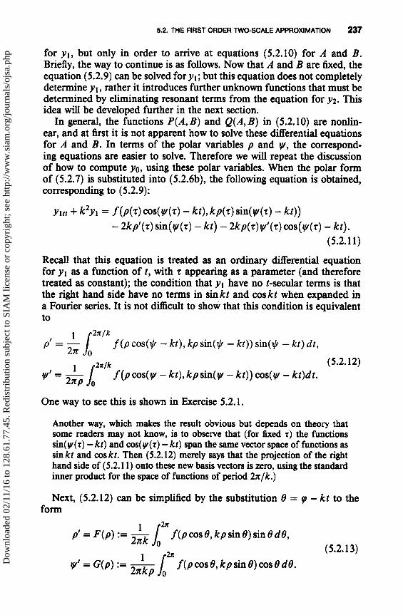
In general, the functions P(A, B) and Q(A, B) in (5.2.10) are nonlin-ear, and at first it is not apparent how to solve these differential equationsfor A and B. In terms of the polar variables p and W, the correspond-ing equations are easier to solve. Therefore we will repeat the discussionof how to compute yo, using these polar variables. When the polar formof (5.2.7) is substituted into (5.2.6b), the following equation is obtained,corresponding to (5.2.9):

Yitt + k2Y1 = ƒ(p(T) cos( ►Y(z) — kt), kp('r) sin(W(r) — kt))

— 2kp'(r) sin(y^(T) — kt) — 2kp(T)yi'(r) cos(yr(T) — kt).(5.2.11)

Recall that this equation is treated as an ordinary differential equationfor y1 as a function of t, with r appearing as a parameter (and thereforetreated as constant); the condition that y1 have no t-secular terras is thatthe right hand side have no terms in sinkt and coskt when expanded ina Fourier series. It is not difficult to show that this condition is equivalentto

p2/1c

p' = 1 J f (p cos(* — kt), kp sin(i — kt)) sin(* — kt) dt,

2x/k (5.2.12)yr' = 21rp 0 f(pcos(yi — kt),kpsin(gr — kt)) cos( yr — kt)dt.

One way to see this is shown in Exercise 5.2.1.

Another way, which makes the result obvious but depends on theory thatlome readers may not know, is to observe that (for fixed z) the functionssin(y^(z) — kt) and cos(W(:) - kt) span the same vector space of functions assin kt and cos kt. Then (5.2.12) merely says that the projection of the righthand side of (5.2.11) onto these new basis vectors is zero, using the standardinner product for the space of functions of period 21r/k.)

Next, (5.2.12) can be simplified by the substitution 0 = q? — kt to theform

1p'= F(p) := ^k 1

2z

f(p cos 0, kp sin 0) sin 9 d0, 2^ (5.2.13)

1yr'=G(p):= 27rkp J f(p cos 0, kp sin 0) cos 0 do.D

ownl

oade

d 02

/11/

16 to

128

.61.

77.4

5. R

edis

trib

utio

n su

bjec

t to

SIA

M li

cens

e or

cop

yrig

ht; s

ee h

ttp://

ww

w.s

iam

.org

/jour

nals

/ojs

a.ph

p

238 MULTIPLE SCALES

These are the promised equations, which are simpler than the correspond-ing equations (5.2.10) in Cartesian variables since F and G depend upononly one variable p, whereas P and Q depend upon both A and B. Al-though both (5.2.10) and (5.2.13) are in general nonlinear, the equationsin (5.2.13) are "solvable by quadrature," that is, the problem of solvingthem is reducible to a problem of integration. Namely, the first equationcan be written in separated form d p/F(p) = dr and integrated, using theinitial condition from (5.2.8); after the solution p(r) is found, the sec-ond equation becomes di/i = G(p(r)) dr, where the right hand side is aknown function of r to be integrated. Provided these two integrations can bedone, the solution is complete.

Of course, since (5.2.10) is equivalent to (5.2.13) by a simple changeof variables, it also is solvable by quadrature although that is not obviousfrom its form. This observation is useful, since the Cartesian form hasa definite advantage when it comes to computing higher approximations(Section 5.3). The procedure for solving (5.2.10) by quadrature will bedeveloped in the examples below.

This completes the heuristic derivation of the first order two-scale ap-proximation. It has already been mentioned that the same approximationwill be derived again, from an entirely different point of view, in Chapter6. The question remains: Does this approximation accomplish its purpose?The answer is yes. The following theorem is proved at the end of Section5.5:

Theorem 5.2.1. For fixed a and fl there exist constants el, c, and T suchthat the exact solution y(t, e) of (5.2.1) satisfies

^y(t,e)—yo(t,et)I <ce for 0<t<T/e, 0<e<el. (5.2.14)

A similar theorem giving more information about T is proved in Chap-ter 6 (Theorem 6.2.2).

Example 5.2.1. A Linear Problem

As a first illustration of the method of multiple scales, we will computethe first approximation to the (exactly solvable) linear problem discussedin Section 5.1:

y+2ey+(1+e)y=0,

y(0) = a, (5.2.15)

y(0)=0.

The desired approximation has already been derived from the exact solu-tion; it is the first term of (5.1.13). Here it will be obtained by followingthe procedures described above. As always, it is more instructive to work

Dow

nloa

ded

02/1

1/16

to 1

28.6

1.77

.45.

Red

istr

ibut

ion

subj

ect t

o SI

AM

lice

nse

or c

opyr

ight

; see

http

://w

ww

.sia

m.o

rg/jo

urna

ls/o

jsa.

php

5.2. THE FIRST ORDER TWO-SCALE APPROXIMATION 239

out each step of the procedure for each application, rather than to applyformulas such as (5.2.10) or (5.2.13) mechanically. Substitution of (5.2.2)into (5.2.15), using (5.2.4), leads to the following sequence of linear initialvalue problems (compare (5.2.6)):

Yott + Yo = 0,

yo(0,0) = a, (5.2.16a)Yot(0, 0) = 0;

Ylu +Yl = — (Yo + 2Yot + 2Yon),yl(0,0) = 0, (5.2.16b)

Ylt(0, 0) = —Yot(0, 0);

Y2tt + Y2 = —(2yoT +Yott +Yl + 2Ylt + 2Yltt),

Y2(0,0) = 0, (5.2.16c)

Y2t(0, 0) _ —YI„(0, 0)•

We will need only the first two of these in this section, but the third willbe used later. The solution of (5.2.16a) in "amplitude/phase" form is

Yo = p(r) cos(W(r) — t),

p(0) = a, (5.2.17)

qr(0) = 0,

where p(z) and yr(T) are as yet undetermined except for their initial con-ditions. The equation for y l now becomes

Yltt +yl = — p(1 + 2w') cos( — t) — 2(p' + p) sin( W — t) . (5.2.18)

Since v is a function of r only, it is treated as a constant while solvingthe equation for y l . Rather than expand the right hand side in a Fourierseries in t, it is more convenient to expand it in yi — t; in fact, it is alreadyexpressed as a Fourier series in yr — t, which contains only two terms, bothof them resonant with the free frequency 1. Therefore the heuristic rulethat t-secular terms should be eliminated compels us to choose p(r) andy^(r) to satisfy

yr'=-1/2.(5.2.19)

The solution of these equations, with the initial conditions given in (5.2.17),are

P(r) =(5.2.20)

W(r) _ —T/2,

Dow

nloa

ded

02/1

1/16

to 1

28.6

1.77

.45.

Red

istr

ibut

ion

subj

ect t

o SI

AM

lice

nse

or c

opyr

ight

; see

http

://w

ww

.sia

m.o

rg/jo

urna

ls/o

jsa.

php

240 MULTIPLE SCALES

leading to the complete first approximation,

yo(t, z) = ae-T cos(-z/2 - t) = ae -T cos(t + z/2). (5.2.21)

Now we will repeat these calculations in Cartesian variables. As re-marked above, it is more difficult to compute the first approximation inCartesian variables than in polar, but for higher approximations the re-verse is true. Therefore it is worthwhile to understand how to compute thefirst approximation in Cartesian variables. Beginning with (5.2.16a), thesolution can be written

yo = A(z) cos t + B(z) sint,

A(0) = a, (5.2.22)

B(0) = 0.

The equation for yl is

yl« + yl = -(A + 2B + 2B') cos t + (-B + 2A + 2A') sin t. (5.2.23)

The right hand side is, once again, already expanded in a Fourier series(this time in t), having two terms, both of which are resonant. The non-secularity conditions are

A' = -A + B/2,(5.2.24)

B'=-A/2--B.

This is a linear system of two differential equations in two unknown func-tions, and can be solved as such, for instante by matrix methods. But itis linear only because the original equation (5.2.15) is linear; so to solve(5.2.24) by linear methods will not help with more general problems. In-stead, observe that by the chain rule and by (5.2.24),

di: B2) = 2AA' + 2BB' = -2(A 2 + B2). (5.2.25)

This equation can be solved for the quantity A2 + B2 :

A2 +•B2 = [A (0)2 + B(0)2] e-2t = (ae- t)2 . (5.2.26)

(Notice that since A2 + B2 = p2 , we have actually introduced polar coor-dinates "on the sly" here. This is the secret of how to solve (5.2.10) byquadrature.) It follows that there exists (z) such that

A(z) = ae-icos^(z),(5.2.27)

B(z) = ae-T sin(z).

Dow

nloa

ded

02/1

1/16

to 1

28.6

1.77

.45.

Red

istr

ibut

ion

subj

ect t

o SI

AM

lice

nse

or c

opyr

ight

; see

http

://w

ww

.sia

m.o

rg/jo

urna

ls/o

jsa.

php

5.2. THE FIRST ORDER TWO-SCALE APPROXIMATION 241

To compute , substitute the first equation of (5.2.27) into the first equa-tion of (5.2.24) to obtain

2A'+2A-B = -a(2^'+ 1) sin = 0

M•II

= -1/2, (5.2.28)

so that (r) = (0) - T/2. (Compare (5.2.28) with the second equation of(5.2.19): c is another "secret" polar coordinate.) The initial value (0) = 0follows from (5.2.22) and (5.2.27), from which

A(T) = ae-T cos 2,(5.2.29)

B(T) = -ae -T sin 2,

givingT Tyo(t, z) = ae't {cos cos t - sin 2 sin t} ,

( 5.2.30 )

in agreement with (5.2.21).

Example 5.2.2. The Van der Pol Equation

For the next example, consider the Van der Pol equation

y+e(y2 - 1)y+y=0,y(0)=c, (5.2.31)

y(0)=O,

which has been studied in Section 4.4. Since this is a nonlinear equation,the exact solution is not available for comparison with the approximationfound by multiple scale methods. However, it has been seen that for smalle there is a unique limit cycle and it is stable. These features can be rec-ognized in the approximate solution by two-timing, which is (see Exercise5.2.2):

y . 2acos t. (5.2.32)

va +(4-a

It is possible to recognize some of the properties of the exact solutionsof Van der Pol's equation in this approximate solution. For instance, ast -> oo in (5.2.32), the transient effect (on the time scale i) dies out, leavingthe periodic solution

y ^` 2 cos t (5.2.33)

Dow

nloa

ded

02/1

1/16

to 1

28.6

1.77

.45.

Red

istr

ibut

ion

subj

ect t

o SI

AM

lice

nse

or c

opyr

ight

; see

http

://w

ww

.sia

m.o

rg/jo

urna

ls/o

jsa.

php

242 MULTIPLE SCALES

which coincides with the Lindstedt approximation to the limit cycle foundin Exercise 4.4.1. Thus the approximate solution exhibits a stable limitcycle close to the exact limit cycle of the Van der Pol equation. One mightwonder why the two-timing approximation is this good; after all, it is onlyintended to be uniformly valid on an expanding interval, not for all time.It turns out that a careful analysis of the error in (5.2.33) shows that whilethe phase W is only approximated well on an expanding interval, the am-plitude p is approximated well for all time. As in the previous example,this is due to damping (or more precisely, to the attracting character of thelimit cycle). In this problem, damping only affects the error in a directionnormal to the limit cycle, and "in-track error" continues to accumulate inthe tangential direction just as it does for the Lindstedt approximation tothe limit cycle. (See Section 4.3 for the notion of "in-track error.") It isnot always permissible to draw conclusions about the behavior of a systemas time approaches infinity from approximate solutions, but when the be-havior in question is sufficiently "strong" in some sense, it will survive inthe approximations. The further exploration of this topic is beyond thisbook; see Notes and References.

Exercises 5.2

1. Derive (5.2.12) from the nonsecularity condition on (5.2.11) by anothermethod than that indicated in the text. Hint: Multiply the right handside of (5.2.11) by sinkt and by coskt, and integrate from 0 to 2n/k.Set the results equal to zero, and use trig identities.

2. Find the first order two-scale approximation for the Van der Pol equa-tion (5.2.30). Do not use the general formulas, but carry out the pro-cedure of substituting (5.2.2) into (5.2.30) and obtaining equations foryo and yl. Use polar form for the solution for yo, and fix p(r) and w(t)by eliminating resonant terms from the equation for yl. After you haveobtained your approximate solution, compare it with the solution toExercise 2.4.4b. Repeat the calculation using Cartesian variables.

3. Find the first order two-scale approximation for the autonomous Duifing equation ,y + y + ey3 = 0, y(0) = a, y(0) = 0. Do the calculation inboth polar and Cartesian variables.

4. Find a leading order approximation (by the multiple scale method) fory + eyy + y = 0, y(0) = 1, 5'(0) = 0. Compare the result with Exer-cise 4.3.6.

5.3* HIGHER ORDER APPROXIMATIONS

In this section (which may be omitted without loss of continuity) we willinvestigate three strategies for finding higher order multiple scale approx-imations. These three strategies have already been mentioned at the end

Dow

nloa

ded

02/1

1/16

to 1

28.6

1.77

.45.

Red

istr

ibut

ion

subj

ect t

o SI

AM

lice

nse

or c

opyr

ight

; see

http

://w

ww

.sia

m.o

rg/jo

urna

ls/o

jsa.

php

5.3* HIGHER ORDER APPROXIMATIONS 243

of Section 5.1, where three types of second order approximations weregiven for the linear initial value problem (5.1.9). Briefly stated, the threeapproaches are: (1) to continue as in Section 5.2 with the two time scalest and r, computing higher order terms in the series (5.2.2); (2) to use twotime scales, but replace t by a "strained" time scale similar to that used inthe Lindstedt method; and (3) to add more time scales besides t and T.

The purpose of the first strategy is to improve the accuracy of the firstapproximation, without attempting to increase the length of time 0(1 /e)for which the approximation is valid. For problems of the form (5.1.1) itcan be shown that the two-time-scale expansion using t and i which wasbegun in the last section can be carried out to any order, and that thesolution (5.2.2) taken through the term yk_ 1 has error Q(8k) on expandingintervals of length 0(1 /e). Thus, at least in theory, the first strategy isalways successful at achieving its goal. However, to carry out the solution inpractice requires solving certain differential equations in order to eliminatesecular terms; these differential equations are in general nonlinear, andtherefore may not have "closed form" solutions (that is, explicit solutionsin terms of elementary functions). So the fact that the solutions are possible"in theory" does not always guarantee that the calculations are possible inpractice, although in many cases they are.

The second and third strategies are more ambitious. Their aim is notonly to improve the asymptotic order of the error estimate, but also toextend the validity of the approximations to "longer" intervals of time,that is, expanding intervals of length 0(1 /e2 ) or longer. In other words,these methods are an attempt to recapture some of the "trade-off" propertyenjoyed by Lindstedt expansions in the periodic case. These methods wereoriginally developed by heuristic reasoning only, and there does not yetexist a fully adequate rigorous theory explaining their range of validity.There are a number of specific problems of the form (5.1.1) for whichthese methods work, or seem to work. There are others for which theydefinitely do not work. Because the situation is not yet fully understood,we will not attempt to state any general results for these strategies, but willillustrate the third strategy briefly and comment on the difficulties.

It should be mentioned that there is another approach to finding higher or-der approximations for these problems, namely the method of "higher orderaveraging" which will be developed in the next chapter. This method doesnot require specifying a set of time scales in advance. Instead, the necessarytime scales appear automatically in the course of solving the problem. Theapproximations constructed by averaging are always valid at least on expand-ing intervals of order 1 /e, and sometimes on longer intervals. It would appearthat this method is the most powerful.

To explain the higher order two-time-scale method using t and T, wewill continue the solution of the linear example (5.2.15) from where it wasleft off in Section 5.2. At that time we had found yo, either in the form

Dow

nloa

ded

02/1

1/16

to 1

28.6

1.77

.45.

Red

istr

ibut

ion

subj

ect t

o SI

AM

lice

nse

or c

opyr

ight

; see

http

://w

ww

.sia

m.o

rg/jo

urna

ls/o

jsa.

php

244 MULTIPLE SCALES

(5.2.21) or (5.2.30). In doing so, we had eliminated resonant terms fromthe right hand side of (5.2.16b) and had in fact found that the entire righthand side was resonant. Therefore we begin with (5.2.16b) in the form

Yin + Y1 = 0,

yl(0,0) = 0, (5.3.1)Yit(0, 0) = a.

Although the polar form was simplest for finding yo, the computationaladvantage seems to lie with the Cartesian form this time, so we write thesolution of (5.3.1) as

y l (t, T) = C(T) cos t + D(T) sin t,

C(0) = 0, (5.3.2)D(0) = a.

As before, the solution is not uniquely determined by the informationavailable, and it is necessary to adopt heuristic reasoning to fix the func-tions C and D completely. Since the error in the approximation y ^_' yo+eylis expected to behave like e2y2, the procedure is to eliminate t-secular termsfrom Y2 so that it remains bounded on expanding intervals of order 1 /e.To this end we examine equation (5.2.16c), which can be written out as

Y2a+Y2 = -{A"+2A'+2D'+C+2D}cost

- {B" + 2B' - 2C' + D - 2C} sin t, (5.3.3)

where A and B are as in (5.2.29), and C and D are as yet unknown.Both terms on the right hand side of (5.3.3) are resonant and must be setequal to zero. Making use of the expressions for A and B, the resultingnonsecularity conditions are

C'=-C+ 1D+ 5ae- t sin 2,(5.3.4)

D'=-1C-D + 5ae-tcos2.

This inhomogeneous linear system of ordinary differential equations issolvable, with the initial conditions given in (5.3.2):

C(r) = ae-t 1 8 T+ i) sin 2,(5.3.5)

D(z)= ae`(8z+1)cos2.Dow

nloa

ded

02/1

1/16

to 1

28.6

1.77

.45.

Red

istr

ibut

ion

subj

ect t

o SI

AM

lice

nse

or c

opyr

ight

; see

http

://w

ww

.sia

m.o

rg/jo

urna

ls/o

jsa.

php

5.3* HIGHER ORDER APPROXIMATIONS 245

When this is substituted into (5.3.2), it is easy to see that yo+ey l coincideswith the approximation (5.1.13) developed from the exact solution.

If we had solved (5.3.1) in polar form y = plcos(yr1 — t), the nonsecularityconditions and initial conditions to be satisfied by pl (T) and vi (T) wouldhave been (after some calculation)

p'+p= 8ae' T sin (W +2),

p(2w'+ 1) = 4ae—t cos (vi+ 2 ) '

p(0) = a,

w(0) =

It is possible to solve these by clever inspection; the solution is

p=ae—T I r +1 I,

w=2-2•

However there does not seem to be any technique behind this, and if oneattempts to solve the original problem (5.2.15) with initial velocity fi in-stead of zero, the polar equation becomes intractable, whereas the analog of(5.3.4) is still an inhomogeneous linear system. This is why we said that theCartesian form seems preferable for this problem. Nevertheless, it must beemphasized that (5.3.4) is linear only because the original problem (5.3.4) islinear, and there is no general procedure for solving the nonsecularity condi-tions that arise in the course of the two-timing method. As mentioned before,the problem is a practical one, not a theoretical one: The nonsecularity con-ditions in the two-timing method (using "unstrained" fast time t and slowtime r) are always initial value problems of a soit which, in theory, have so-lutions, although they may not be solvable in "closed form" using elementaryfunctions.

The method to be investigated next has been used to solve a numberof applied problems and is quite popular in the engineering literature.However, it rests on quite shaky foundations from a mathematica) pointof view. The purpose of the following example is not so much to teachthe method, as to discuss it and point out some of the difficulties with it.Anyone wishing to learn the method for practical use wil) have to studymany examples from the literature to see how these difficulties are dealtwith on an ad hoc basis in different situations.

The problem we will study is once again the linear example (5.2.15).The solution wil) be sought in the form

y ~ Yo(t, T, a) + eyl (t, T, a) + e2Y2(t, T, a), (5.3.6)

Dow

nloa

ded

02/1

1/16

to 1

28.6

1.77

.45.

Red

istr

ibut

ion

subj

ect t

o SI

AM

lice

nse

or c

opyr

ight

; see

http

://w

ww

.sia

m.o

rg/jo

urna

ls/o

jsa.

php

246 MULTIPLE SCALES

where T = et and a = eet. Working with the operator equation

dt8t +E 8T +E2= ^ '

one obtains the following sequence of differential equations and initialconditions:

Yott + Yo = 0,

yo(0, 0, 0) = a, (5.3.7a)Yot(0, 0, 0) = 0;

Ytn +Yt = — (Yo + 2Yot + 2Yott),

yl (0, 0, 0) = 0, (5.3.7b)

Yit(0, 0, 0) _ —Yot(0, 0, 0);

Y2tt + Y2 = —(2Yot + Yo + 2Yota +Y1 + 2y1t + 2Y1tz),

Y2(0, 0, 0) = 0, (5.3.7c)

Y2t(0, 0, 0) _ —y1(0, 0, 0) — Y0a(0, 0, 0)•

These equations are very similar to (5.2.16), the only differences being thatthe initial conditions occur at (0, 0, 0) rather than (0, 0) and that (5.3.7c)has additional terms involving derivatives with respect to o. Therefore thesolution of these equations proceeds very much like that of (5.2.16) until(5.3.7c) is reached. It is only necessary to remember that each function isallowed to depend on a. Thus, the solution of (5.3.7a) is

yo=A(i,a) cos t+B(T,a) sin t, (5.3.8)

with

A(0,0) = a,

B(0,0) = 0;

compare (5.2.22). Then it is possible to follow through the steps from(5.2.23) to (5.2.26) almost exactly, except that A' and B' must be writtenAt and BT because they depend also on a, and in (5.2.25) one has . Inplace of (5.2.27), one gets

A(; c) = K(a)e -T cos ^(r, a),

B(i, a) = K(a)e- t sin (T, a),

where

K(0) = a,

(0,0) = 0.

Dow

nloa

ded

02/1

1/16

to 1

28.6

1.77

.45.

Red

istr

ibut

ion

subj

ect t

o SI

AM

lice

nse

or c

opyr

ight

; see

http

://w

ww

.sia

m.o

rg/jo

urna

ls/o

jsa.

php

5.3* HIGHER ORDER APPROXIMATIONS 247

As in (5.2.28), = -1/2; therefore

(T,a)_i(ci) 2

for lome function (a) satisfying n(0) = 0. Putting (5.3.8) together withthe results just obtained, one finds that at this point yo is given by

yo(t, i, o) = K(a)e- T cos (t + 2 - n(Q)) , ( 5.3.9)

where K and rj are as yet unspecified functions satisfying

K(0) = a,n(0) = o.

Here we see the first serious difference between this method and the two-scale method: in the Jatter, yo is completely specified when the resonantterras are eliminated from the yl equation, while in the present methodthere is a dependence on a which is not yet determined.

Having eliminated the resonant terms from the yl equation, one is leftwith

Yitt +Yt = 0,yl (0, 0, 0) = 0,Y11(0, 0, 0) = a,

resembling (5.3.1). In solving (5.3.1) by (5.3.2), we used cos t and sin t as afundamental set of solutions, but in the present case later calculations willbe simplified if we use the cosine and sine of the quantity t + T/2 - (ai)appearing in (5.3.9); this is permissible since for fixed i and a these arelinearly independent solutions of the differential equation. Therefore wewrite

y, (t, r, a) = C(i, a) cos(t + - n(o)) + D(i, a) sin(t + 2 - ,(a)). (5.3.10)

It is easy to check (using the fact that i(0) = 0 and the initial conditionsfor y l ) that

C(0,0) = 0,D(0, 0) = a.

Until now the calculations have been routine. We are now rapidly ap-proaching the point at which the fundamental nature of the method (and

Dow

nloa

ded

02/1

1/16

to 1

28.6

1.77

.45.

Red

istr

ibut

ion

subj

ect t

o SI

AM

lice

nse

or c

opyr

ight

; see

http

://w

ww

.sia

m.o

rg/jo

urna

ls/o

jsa.

php

248 MULTIPLE SCALES

its difficulties) will become clear. Substituting (5.3.9) and (5.3.10) into theright hand side of (5.3.7c), one obtains the following equation for y2 :

y2tt + y2 = [ (4 - 2ri') Ke-' - 2 (D + DT)l cos(t + 2 - n)

+ [2K'e-T + 2 (C + CT)] sin(t + - ri). (5.3.11)

Here, of course, the prime denotes a derivative with respect to a, since it isapplied to functions of a alone. In order that Y2 will contain no t-secularterms (terms proportional to t), the resonant terms must be eliminatedfrom the right hand side of (5.3.11), as usual. Since the entire right handside is resonant, the coefficients of the cosine and sine terms must vanish,leading to the equations

Cr = —C — K'e`,

Dt = -D + 5 ' Ke.(5.3.12)

This provides differential equations for C and D once K and , are known,but is of no help in determining the Jatter functions which are stil un-known. It is clear that a new principle is required, besides the avoidanceof t-secular terras, which will serve to determine K and n.

Recall the reason for avoiding t-secular terms: A term proportional to twill grow with time (assuming the other factors do not approach zero) andwilt become of order 1 /e at the end of an expanding interval of length 1 /e.If a term of formal order e" is t-secular, its actual order on the expandinginterval is e"- 1 , and the series fails to be uniformly ordered. Now the aimof a three-scale method is to achieve uniform validity on an expandinginterval of length 1/e2 . On an interval of this length, a r-secular term willproduce the same type of disordering that a t-secular term produces onthe shorter expanding interval. Now it is clear from (5.3.9) that t-secularterms cannot arise in yo. (And in any case, according to the definition ofuniform ordering in Section 1.8, the leading term of a perturbation seriesdoes not matter.) So the first possibility for such a term occurs in y l ; andin fact yl will contain a z-secular term if and only if C or D contains sucha term. So we propose the following rule: K(o) and rj(o) should be chosenin such a way that the solutions C and D of (5.3.12) contain no T-secularterms.

We will now test this proposed rule by examining the solutions of(5.3.12). Remember that the coefficients K' and (5/8 - ,') are functionsof a alone and therefore may be treated as constants in solving (5.3.12)for C and D as functions of t. Now it is apparent that the "forcing" termsproportional to e produce a response proportional to Te-t; this can beseen by explicitly solving the equations, or by the fact that the associatedhomogeneous equations have a solution proportional to e -T and so the

Dow

nloa

ded

02/1

1/16

to 1

28.6

1.77

.45.

Red

istr

ibut

ion

subj

ect t

o SI

AM

lice

nse

or c

opyr

ight

; see

http

://w

ww

.sia

m.o

rg/jo

urna

ls/o

jsa.

php

5.3* HIGHER ORDER APPROXIMATIONS 249

forced equations respond with an additional factor of T. Now a term of theform re- t is often considered as a T-secular term. In fact, we shall showbelow that this is not the case; but for the moment let us regard this termas something to be avoided, because it contains a factor of T. In order toavoid this term it is necessary to take

K'=0,(5.3.13)

With the initial conditions, this implies

K(a) = a,

,i(a) _ 0.

Finally, then, yo is completely determined:

Yo=ae -Z cos(t +2- ), (5.3.14)

in agreement with the first term of the expansion (5.1.16) derived fromthe exact solution.

Although it appears that we have solved this problem successfully, thereis a difficulty: As hinted above, the term re-" is not actually a r-secularterm. To understand why, recall the precise meaning of a secular term: aterm that is unbounded (on the domaio of interest) and therefore causesthe perturbation series to be not uniformly ordered. Now te-t attains amaximum and then decreases to zero as z approaches infinity. Thereforeit is not secular, either on an expanding interval or indeed on the entirereal line. It follows that in fact there is no need to impose the conditions(5.3.13) which we used to determine K and rl. It is convenient to do so,because these conditions simplify the equations (5.3.12). But we wouldhave obtained just as good a solution (as far as the presence of secularterms is concerned) had we made any choice at all for K and . Theultimate reason that K and are not unique in this problem is that threescales are not actually needed to solve it: We have already pointed out inSection 5.1 that the two-scale solution for this problem is in fact valid forall time, because of the damping.

In the literature, one finds at least three justifications given for requiring(5.3.13) in this problem. One is that it simplifies the equations (5.3.12).Another is that it eliminates the term re`, which is considered as a badterm merely because it looks secular. The third is that it makes the ratio yl /yobounded. If yl contains a term proportional to re— ', then indeed this ratiois unbounded; but this is not harmful. The demand that y„ + 1 /y„ be boundedcomes from the idea that the n + 1 st term of a perturbation series should besmall compared to the nth term. But a careful study of the requirements for

Dow

nloa

ded

02/1

1/16

to 1

28.6

1.77

.45.

Red

istr

ibut

ion

subj

ect t

o SI

AM

lice

nse

or c

opyr

ight

; see

http

://w

ww

.sia

m.o

rg/jo

urna

ls/o

jsa.

php

250 MULTIPLE SCALES

uniform asymptotic validity (see the discussion surrounding Theorem 1.8.1)shows that the correct concept of uniform ordering involves the boundednessof the coefficients and not of their ratios. So in the present problem the onlyvalid justification of (5.3.12) is the first: that it simplifies the equations.

In the foregoing discussion we have emphasized repeatedly that in thisproblem the requirement to eliminate r-secular terms does not determine Kand rl uniquely. In general, there are three a priori possibilities, all of whichdo in fact occur in specific problems: There may be a unique solution thatis free of r-secular terms; there may be many solutions that are free of theseterms (as in the problem treated above); or there may be no solution that isfree of these terms. Clearly nonuniqueness of the solution (as in our case)is not a serious drawback for a method. What is most disconcerting aboutthe three-scale method is the existence of problems for which the equationscorresponding to (5.3.12) have no solutions that are free of r-secular terms.When this is encountered, the method simply fails. An example of sucha problem is the following equation, which combines a "Duffing term" oforder e with a "Van der Pol term" of order e 2 :

y + e2 (y2 — 1)y + y + ey3 = 0. (5.3.15)

The ambitious reader may wish to attempt a three-scale solution of thisproblem, although the calculations are formidable (and are best handledwith a notation that uses complex variables). But the fact is that at the endone finds there is no way to eliminate secular terms. (A reference is givenin Section 5.7.) At this point there is no general theory that would explainwhy the method fails for some problems and succeeds with others.

In cases for which the three-scale method works (formally), the resultingseries is uniformly ordered on expanding intervals of length 1 /e2 . This initself does not imply that the series is uniformly valid on these intervals;as usual, uniform ordering of the terms in the series says nothing aboutthe error. But it is at least plausible that such solutions are uniformlyvalid. We will not address the question of error estimation for the methodsdiscussed in this section, but will prove the validity of the first order two-scale approximation in Section 5.5.

5.4. PERIODIC STANDARD FORM

All of the differential equations considered in Chapter 4 and in this chap-ter, and a great many others, can be put into the form

i= ef(x, t, e) = efl (x, t) + e2f2(x, t) + • • • , ( 5.4.1)

where x is an N-dimensional vector and f is an N-vector-valued functionthat is periodic in t with period independent of e. Usually the period isassumed to be 2n; this can always be achieved by changing the unit of time.

Dow

nloa

ded

02/1

1/16

to 1

28.6

1.77

.45.

Red

istr

ibut

ion

subj

ect t

o SI

AM

lice

nse

or c

opyr

ight

; see

http

://w

ww

.sia

m.o

rg/jo

urna

ls/o

jsa.

php

5.4. PERIODIC STANDARD FORM 251

This section is entirely concerned with the procedure for achieving theform (5.4.1), which we call periodic standard form, and which is frequentlyreferred to in the literature as standard form for the method of averaging.(There are actually several standard forms used in averaging and multiplescale methods, some of which will appear later, and we distinguish these bycalling them periodic standard form, quasiperiodic standard form, angularstandard form, and so forth.) The section is organized into examples; eachexample is a general class of equations, rather than a concrete instance.The first few examples are types of equations which have been consideredbefore. After these, new types of problems are introduced, including some(for illustrative purposes) which cannot be put into standard form.

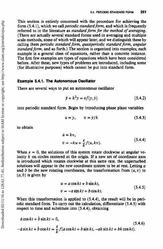
Example 5.4.1. The Autonomous Oscillator

There are several ways to put an autonomous oscillator

y + k2y = ef(y,y) (5.4.2)

into periodic standard form. Begin by introducing phase plane variables

u = y, v=y/k (5.4.3)

to obtain

ü = kv,E

v=—ku+kf(u,kv).(5.4.4)

When e = 0, the solutions of this system rotate clockwise at angular ve-locity k on circles centered at the origin. If a new set of coordinate axesis introduced which rotates clockwise at this same rate, the unperturbedsolutions will appear in the new coordinate system to be at rest. Letting aand b be the new rotating coordinates, the transformation from (u, v) to(a, b) is given by

u = a cos kt + b sin kt,(5.4.5)

v = —asinkt + b cos kt.

When this transformation is applied to (5.4.4), the result will be in peri-odic standard form. To carry out the calculation, differentiate (5.4.5) withrespect to time and substitute into (5.4.4), obtaining

ácoskt+bsinkt=0,(5.4.6)

—á sin kt + b cos kt = k f(a cos kt + b sin kt, —ak sin kt + bk cos kt).Dow

nloa

ded

02/1

1/16

to 1

28.6

1.77

.45.

Red

istr

ibut

ion

subj

ect t

o SI

AM

lice

nse

or c

opyr

ight

; see

http

://w

ww

.sia

m.o

rg/jo

urna

ls/o

jsa.

php

252 MULTIPLE SCALES

Now solve this system for á and b (by, for example, multiplying the firstequation by cos kt and the second by — sin kt and adding) to obtain

á = — k f(acoskt+bsinkt,—aksinkt+bkcoskt)sinkt,(5.4.7)

b=+kf(acoskt+b ski kt, —ak sin kt+bk cos kt)coskt.

The right hand side of this system is periodic in t with period 2n /k,and contains a factor of e; it is therefore in periodic standard form withx = (a, b). Note that the function f is constructed from f as specified onthe right hand side of (5.4.7); in particular, the lightface letter f does notdenote the magnitude (norm or length) of the boldface vector f, a conven-tion common in physics. Instead we regard f as an entirely separate letterfrom f, and define it as needed in each example. (In this book the normof a vector v is denoted IIvII, as usual in mathematics.)

Another way to put (5.4.2) into standard form is to introduce polarcoordinates into the phase plane before rotating. Setting

u = r cos O,(5.4.8)

v = rsin0

in (5.4.4) leads to

i= k f(r cos 0, kr sin 0) sin 0,(5.4.9)

= —k+ kr f(rcos0,krsin0)cos0.

(A specific example of this computation is given below; see the steps from(5.4.17) to (5.4.18).) To rotate polar coordinates at angular velocity k inthe clockwise direction it is only necessary to change the angular variable,leaving the radial variable as it is: setting

0=0 —kt (5.4.10)

yields

r = k f (r cos(ip — kt), kr sin(ip — kt)) sin(rp — kt),(5.4.11)

Ir f (r cos(9 — kt), kr sin(rp — kt)) cos(rp — kt),

which is in periodic standard form with x = (r, q). (Do not forget, inchecking that an equation is in periodic standard form, to check both thatit is periodic and that it contains the factor e.)

The crucial step in arriving at the periodic standard forms (5.4.7) and(5.4.11) is to make a change of variables which "removes" the unperturbed

Dow

nloa

ded

02/1

1/16

to 1

28.6

1.77

.45.

Red

istr

ibut

ion

subj

ect t

o SI

AM

lice

nse

or c

opyr

ight

; see

http

://w

ww

.sia

m.o

rg/jo

urna

ls/o

jsa.

php

5.4. PERIODIC STANDARD FORM 253

solution, that is, renders the unperturbed solution constant (in the newvariables). In the present example, it is easy to see how to remove theunperturbed solution: Since that solution is a rotation, it is only necessaryto rotate the coordinaten at the same rate. When it is not obvious howto proceed, the following strategy is useful: First find the general solutionof the reduced problem, which will contain arbitrary constants, and thenreinterpret this solution as a change of variables (the new variables beingthe "constants"). In the present case, the solution of (5.4.4) with e = 0 is(5.4.5) with a and b constant, or else

u = rcos(rp — kt),(5.4.12)

v = r sin( — kt),

with r and q constant. Using (5.4.5) as a coordinate change (with a and bas the new variables) leads to (5.4.7), and using (5.4.12) leads to (5.4.11).

The idea of using the unperturbed solution to define a change of variablesis closely related to the method of variation of constants (or variation ofparameters). In Appendix C, it is shown that the usual method of variation ofconstants (for second order inhomogeneous linear differential equations) canbe regarded as a change of variables. We will now show that the changes ofvariables used above can be regarded as a variation of constants, and that inthis way it is possible to achieve both of the periodic standard forms (5.4.7)and (5.4.11) directly from the second order equation (5.4.2) without firstintroducing the phase plane variables u and v. We will not make much useof this method, since we regard the previous methods as more conceptuallyclear, but variation of parameters is commonly seen in the literature. Onebegins with the solution of (5.4.2) when e = 0, which can be written in theform

y = acoskt + bsinkt, ( 5.4.13)

where a and b are constants. The derivative of (5.4.13) is, of course,

,y = —ak sin kt + bk cos kt. (5.4.14)

The idea of variation of constants is to look for the solution of the perturbedproblem (5.4.2) in the form (5.4.13) by allowing a and b to become functionsof t rather than constants. Since it requires two conditions to determinethe two unknown functions a and b, it is permissible to impose (5.4.14) asa condition on a and b in addition to the requirement that (5.4.13) solve(5.4.2); this is equivalent to

k cos kt + b sin kt = 0. (5.4.15)

Substituting (5.4.13) and (5.4.14) into (5.4.2) leads directly to (5.4.7), byalgebraic steps similar to those carried out above. A similar analysis beginringwith y = rcos(q — kt) leads to (5.4.11).

Dow

nloa

ded

02/1

1/16

to 1

28.6

1.77

.45.

Red

istr

ibut

ion

subj

ect t

o SI

AM

lice

nse

or c

opyr

ight

; see

http

://w

ww

.sia

m.o

rg/jo

urna

ls/o

jsa.

php

254 MULTIPLE SCALES

In order to understand the procedures leading to periodic standard form,it is important to follow the steps in some specific examples. We will there-fore put the Van der Pol equation

g+ e(y2 — 1)y + y = 0 (5.4.16)

into periodic standard form. First write (5.4.16) as a system with u = y,v=y:

u =v,(5.4.17)

v = — u + E(1 — u2 )v.

Then differentiate (5.4.8) and substitute into (5.4.17), obtaining

r cos 0 — r9 sin 0 = r sin 0,

ksin0 +r9cos0 = —rcos8 +e(1 — r2 cos2 9)rsin0.

Multiplying these equations by cos 0 and sin 0, and adding or subtracting,gives

r = e(1 — r2 cos2 9)r sin2 9,(5.4.18)

9 = — 1 +e(1 — r2 cos2 0)sin0cos0.

(Notice the division by r in obtaining the second equation.) Now (5.4.10)gives the periodic standard form (remember k = 1):

r = e (1 — r2 cos2 (rp — t)) r sin2 (q, — t),(5.4.19)

rp = e (1 — r2 cos2 (9 — t)) sin(gp — t) cos( rp — t).

Additional practice with these ideas will be found in Exercises 5.4.1, 5.4.2,and 5.4.3.

Example 5.4.2. Harmonic Resonance

The periodically forced nearly linear oscillator is

y + k2y = ef (y, y, cv(e)t), (5.4.20)

where f is periodic of period 2n in its third argument and therefore ofperiod 2n /w(e) in t. Consider the harmonie resonance case (defined inSection 4.5) for equation (5.4.20), that is, the case in which the forcingfrequency reduces to the free frequency when e = 0:

w(e)— k +eo),+e2cv2+•••. (5.4.21)

Dow

nloa

ded

02/1

1/16

to 1

28.6

1.77

.45.

Red

istr

ibut

ion

subj

ect t

o SI

AM

lice

nse

or c

opyr

ight

; see

http

://w

ww

.sia

m.o

rg/jo

urna

ls/o

jsa.

php

5.4. PERIODIC STANDARD FORM 255

Since the unperturbed form of (5.4.20) is the same as that of (5.4.2), it istempting to try the same coordinate transformations (5.4.5) and (5.4.12)which lead to periodic standard form in the previous example. However,the result of applying (5.4.5) to (5.4.20) is

á = — k f (a cos kt + b sin kt, —ak sin kt + bk cos kt, w(e)t) sin kt,

b =+kf (a cos kt + b sin kt, —ak sin kt + bk cos kt, w(e)t) cos kt,

which is not in periodic standard form because the right hand side is notperiodic in t (unless w(e) _— k). This periodicity can be recaptured bymodifying the angular velocity at which the coordinates are rotated whene 0 0. Namely, if (5.4.5) is replaced by

u = a cos to(e)t + b sin to(e)t,(5.4.22)

v = —a sin w(e)t + b cos w(e)t,

which reduces to (5.4.5) when e = 0, then the result of transforming(5.4.20) is

á = —b (cw(e) — k) — k f (u, kv, w(e)t) sin w(e)t,(5.4.23)

b = +a (w(e) — k) + k ƒ(u, kv, w(e)t) cos to(e)t,

where u and v are being used not as separate variables but as "stand-ins"for the expressions given by (5.4.22), in order to shorten the equations.This system is nearly in periodic standard form, except that the period ofthe right hand side is 2n/cw(e), which depends upon e. For some purposesthis is satisfactory, but in order to eliminate the e dependence from theperiod it is only necessary to introduce the strained time

t+ = w(e)t. (5.4.24)

Then (5.4.23) becomes

da — —b cw(e)—kd t+ — w(e)

ekco(e) f (a cos t+ + b sin t+, —ak sin t+ + bk tost+, t+) sin t+

db — + a w(e)—kdt+ w(e)

(5.4.25)

e+ koxe) f (a cos t+ + b sin t+, —ak sin t+ + bk cos t+, t+) cos t+Dow

nloa

ded

02/1

1/16

to 1

28.6

1.77

.45.

Red

istr

ibut

ion

subj

ect t

o SI

AM

lice

nse

or c

opyr

ight

; see

http

://w

ww

.sia

m.o

rg/jo

urna

ls/o

jsa.

php

256 MULTIPLE SCALES

which can be expanded, using (5.4.21), into

dadt+

—k {boel+kf(a cost+ +bsint+,—aksint++bkcost+,t+)sint+}

+0(82 ),

db (5.4.26)

d t+ _

+ k 1aco 1 + kf(acost+ + b sin t+, —ak sint+ + bk cos t+, t+) cos t+ }

+ O(e2 ).

This is in periodic standard form. It would not have been correct to ex-pand in e prior to introducing t+, because this would have destroyed theperiodicity (since the period in t depends upon e). The essential point inachieving periodic standard form for this problem is to use (5.4.22). In Ex-ample 5.4.1, the coordinate change that leads to periodic standard form isthe solution of the unperturbed equation. In the present example, (5.4.22)has built into it both the solution of the unperturbed equation (to whichit reduces when e = 0) and the perturbation frequency w(e). If variationof constants is used, it is necessary to modify the postulated form of thesolution in the same way. (Exercise 5.4.4.)

Similarly, it is possible to obtain a periodic standard form in polarcoordinates. Setting

u = rcos(q> — to(e)t),(5.4.27)

v = r sin (9 — to(e)t)

results in

r = k f (u, kv, to(e)t) sin (, — to(e)t) ,(5.4.28)

= (w(e) — k) + kr f (u, kv, to(e)t) cos (rp — w(E)t) + 0(82 ),

where this time u and v stand for the expressions given in (5.4.27). (SeeExercise 5.4.5.) Upon introducing t+ and expanding in e, this gives

d+ = k2 f (r cos(ip — t+), kr sin( ~ t+), t) sin(, — t+) + 0(82 ),

(5.4.29)

d = k { w1 + krf (rcos(CD — t+), krsin(9p — t+), t) cos(ip _t+)}

+ 0(e2),

which is in periodic standard form.

Dow

nloa

ded

02/1

1/16

to 1

28.6

1.77

.45.

Red

istr

ibut

ion

subj

ect t

o SI

AM

lice

nse

or c

opyr

ight

; see

http

://w

ww

.sia

m.o

rg/jo

urna

ls/o

jsa.

php

5.4. PERIODIC STANDARD FORM 257

As an illustration of periodic standard form for a forced oscillator inharmonic resonance, consider the weakly forced and damped Duffing equa-tion

,y + eal,y + y + e#%jy3 = eyl cos co(e)t. (5.4.30)

Here k = 1, so u = y and v = ,y, and by comparison with (5.4.20),

f(u,v,t+ ) = 71 colt+ —2lu 3 —C 1v.

Therefore the periodic standard form in polar coordinates (5.4.24) is inthis case

drdt+ _

e {yl cos t+ sin(rp —t) — A,1 r3 cos3 (rp — t+) sin(rp — t+) — 8 1 r sin2 (rp — t+) }

+0(e2 ),drpdt+

(5.4.31)

s {cvl + rl cos t+ cos(ip — t+) —),1r2 cos4(f — t+ ) — 81 cos(gy — t) sin( — t+)}

+ O(e2 ).

The reader should obtain these equations by working through the stepsleading to (5.4.29) beginning with (5.4.30). See Exercise 5.4.6. Anotherway to obtain a periodic standard form for (5.4.20) is given in Exercise5.4.7.

Similar periodic standard forms are possible for subharmonie, super-harmonic, and supersubharmonic resonances. In nonresonant cases, whenw(0)/k is not rational, it is not possible to achieve periodic standard foren.In this case either quasiperiodic standard form or angular standard formmay be used; these forms will be mentioned again in the next example,but serious consideration of them is deferred to Chapter 6.

Example 5.4.3. Coupled Autonomous Oscillators

Consider the following system of coupled autonomous oscillators:

j) +k?Yi = Ef (Y1,...,YN,.Y1,...,YN) (5.4.32)

for i = 1, ..., N. When e = 0, these oscillators are uncoupled, each havingits own free frequency kt . Following the ideas in Example 5.4.1, phaseplan variables

u; := y;, vi := ,y;/k; (5.4.33)

Dow

nloa

ded

02/1

1/16

to 1

28.6

1.77

.45.

Red

istr

ibut

ion

subj

ect t

o SI

AM

lice

nse

or c

opyr

ight

; see

http

://w

ww

.sia

m.o

rg/jo

urna

ls/o

jsa.

php

258 MULTIPLE SCALES

may be introduced for each oscillator, and polar coordinates r ; and 9;defined by

ui = ri cos 9i,(5.4.34)

v i = r; sin O.

In these coordinates the system looks like

ri = k! f (r, cos 8k,.. ., rN cos 9N, kl r, sin 8k, ..., kNrN sin 6N) sin Bi,

E (5.4.35)6; = –k; + — f (rl cos Ok,. .., kNrN sin 9N) cos 8.

kl ri

This is a form which will appear again in Chapter 6, and will be calledangular standard form. If we continue as in Example 5.4.1, rotating eachphase plane at its own angular velocity ki by introducing

gij := 9; + kit, (5.4.36)

the result is

ri = 1l f (r, cos(ç1 — kl t),. .. , kNrN sin(q N — kNt)) sin( ; — kit),

(5.4.37)O; = k , f (r, cos(rp1 — kl t),.. . , kNrN sin(rDN — kNt)) cos(rp; — kt).

The right hand side is not periodic unless all of the free frequencies k; areequal, or at least are all integer multiples of a single frequency K:

k; = miK. (5.4.38)

In this case, (5.4.37) is in periodic standard form with period 2n/K. Oth-erwise, the right hand side of (5.4.37) is what is called a quasiperiodicfunc-tion, and (5.4.37) is said to be in quasiperiodic standard form. A quasiperi-odic function is one which results from the combination of finitely manyperiodic components with different periods. (This is a special case of an al-most periodic function, which allows for infinitely many different periods.)We will not discuss multiple scale methods for quasiperiodic or angularstandard forms, but averaging methods for these cases will be introducedin Chapter 6.

Dow

nloa

ded

02/1

1/16

to 1

28.6

1.77

.45.

Red

istr

ibut

ion

subj

ect t

o SI

AM

lice

nse

or c

opyr

ight

; see

http

://w

ww

.sia

m.o

rg/jo

urna

ls/o

jsa.

php

5.4. PERIODIC STANDARD FORM 259

Example 5.4.4. The Duffing Equation with Strong Forcing

Recall from Section 4.7 that the general form of Duffing's equation innatura! (but already nondimensionalized) parameters is

y+óy+y+2y3 = ycoswt,y(0) = a, (5.4.39)

$, (0) =0.

Until now, the perturbation families that we have considered for (5.4.39)have always involved weak forcing, that is, y has been made into a functionof e in such a way that y(0) = 0. Usually we have taken y(e) = ey, forsimplicity, although it is equally possible to take y(e) = eyl + E2 y2 + • • •,

as in (4.7.2). Now we will consider what happens under the assumption ofstrong forcing, that is, y(e) = yo + ey l + • • • with yo 54 0; for simplicity, wewill assume y(e) = yo. The parameters E and 2 will be taken to be small asusual, so the differential equation to be considered is

y+e81,y+y+e2iy 3 = yo cos cv(e)t. (5.4.40)

The reduced problem for this equation is

y+y = yocosw(0)t, (5.4.41)

which behaves quite differently according to whether co(0) = 1 (the har-monic resonance case) or w(0) 1. In the former case, all solutions of(5.4.41) are unbounded (since they contain a term with a factor of t). It isnot possible to attain periodic standard foren in this case.

In the Jatter case, all solutions of (5.4.41) are bounded and are the sumof two periodic functions, one having frequency 1 and the other w(0).Such solutions are periodic if these two periodic terms have a commonperiod; this happens whenever w(0) = p/q is a rational number other than1. Under these circumstances, that is, in the nonharmonic resonance case,periodic standard foren can be achieved. As an illustration, consider thethird subharmonic problem

co(e) = 3 + eco . (5.4.42)

In this case the general solution of the reduced problem (5.4.41) can bewritten

Y=acost+bsint— 8 cos3t, (5.4.43)

with a and b constant. Our previous experience suggests that somethingsimilar to (5.4.43) should be used as a variation-of-constants solution forthe perturbed problem (5.4.40); more precisely, the correct form should

Dow

nloa

ded

02/1

1/16

to 1

28.6

1.77

.45.

Red

istr

ibut

ion

subj

ect t

o SI

AM

lice

nse

or c

opyr

ight

; see

http

://w

ww

.sia

m.o

rg/jo

urna

ls/o

jsa.

php

260 MULTIPLE SCALES

reduce to (5.4.43) when e = 0 but should have period depending on e insuch a way as to be entrained to the forcing frequency w with entrainmentindex e = 3; in other words the period should equal6n/w. In order to findthe correct form, we will use the strategy developed for the harmonic casein Exercise 5.4.7. Namely, write (5.4.40) in the form

+ 92 2_9y= YoCOS (Ot + 9 y—e81Y—eAly 3, (5.4.44)

where w is given by (5.4.42). All of the terms on the right hand side,except for the first, are small of order e, and the new "free frequency" onthe left hand side matches the expected solution frequency. Now set e = 0to obtain the reduced equation in the form

w2y+ --y = yocoswt. (5.4.45)

This is exactly the same as (5.4.41), considering that co = 3 when e = 0;however, by retaining co (and not replacing it by 3) the general solution of(5.4.45) will still have the correct frequency when e 0. (1f this all seemsslightly mystical, remember that once the correct change of variables isfound, it will justify itself.) The general solution of (5.4.45) is

y= a cos 3 t+ b sin 3 t— 8 2 cos wt. (5.4.46)

Again, this is actually the same as (5.5.43) when e = 0, but now it hasthe correct form for a variation-of-constants solution when e 0. (Sur-prisingly, perhaps, one cannot get the right form just by modifying thefrequencies in (5.5.43); there is also a change in the coefficient of the thirdterm.)

From here the sailing is smooth, although tedious. One allows a andb to become variables, while imposing the usual condition that the firstderivative of (5.4.46) be the same as if a and b were constants; that is tosay, one sets

á cos 3t+bsin 3t=0

and proceeds to differentiate (5.4.46) twice and use (5.4.44) to obtain asecond equation for á and b. The final result is that

á = —ef(a, b, t, e) sin co(e)

t+O(e2 ),(5.4.47)

0(e)

b = +ef(a,b,t,e)cos t+O(e2),

Dow

nloa

ded

02/1

1/16

to 1

28.6

1.77

.45.

Red

istr

ibut

ion

subj

ect t

o SI

AM

lice

nse

or c

opyr

ight

; see

http

://w

ww

.sia

m.o

rg/jo

urna

ls/o

jsa.

php

5.4. PERIODIC STANDARD FORM 261

where

2 w wf(a,b,t,e) = wi (acos 3 t+bsin Yo3 t- coscot)

-ô1 (-a sin 3 t + b cos 3 t + g sin cvt)

3-Al ^acos

CL) t+b sin 3 t- 8 cos cwt) , (5.4.48)

with (of course) w again given by (5.4.42). In obtaining (5.4.48) we havereplaced co by 3 everywhere except inside the trig functions, since the errorcommitted by doing so belongs to the O(e 2 ) terms in (5.4.47). Now (5.4.47)is in periodic standard form, except that one may still wish to introduce astrained time t+ to make the period independent of e.

To understand the idea of a third subharmonic, consider what it meansfor the forcing to undergo three cycles while the solution goes through one.Imagine, for instance, pushing a child on a swing. One usually pushes thechild with a harmonic resonance, pushing once for each period. But aneccentric swing-pusher might try a cycle of push-pull-push as the childgoes forward, pull-push-pull as the child swings back. Since the push pre-dominates during the forward phase, and the pull predominates duringthe return phase, the overall input of energy acts to sustain the swingingmotion against air resistance or other damping forces. Therefore it seemsreasonable that a third subharmonic problem such as (5.4.42) might haveperiodic solutions. It has been shown in Exercise 4.7.3 that there are noperiodic solutions to the third subharmonic problem when the forcing issmall, at least when damping is present. Using the periodic standard formpresented above, together with the methods of Section 6.3 below, it can beshown that periodic solutions do exist when the forcing is strong.

Exercises 5.4

1. Put the Van der Pol equation (5.4.16) into the periodic standard form(5.4.7) in Cartesian coordinates. Do this by following through the stepsleading to (5.4.7), as we did in (5.4.17)-(5.4.19) for the polar form.

2. Put the free Duffing equation ,y + y + ey 3 = 0 into periodic standardform in both Cartesian and Polar coordinates.

3. Repeat the derivation of (5.4.19) from (5.4.16), this time using varia-tion of constants, beginning with (5.4.13) and (5.4.14) with k = 1.

4. Derive (5.4.26) by variation of constants. Begin by looking for a solutionof (5.4.20) in the form y = a cos w(e)t + b sin to(e)t, where a and b arefunctions of t. (When a and b are constants and e = 0, this expressionreduces to the solution of the unperturbed equation; it also has the

Dow

nloa

ded

02/1

1/16

to 1

28.6

1.77

.45.

Red

istr

ibut

ion

subj

ect t

o SI

AM

lice

nse

or c

opyr

ight

; see

http

://w

ww

.sia

m.o

rg/jo

urna

ls/o

jsa.

php

262 MULTIPLE SCALES

correct frequency when e 54 0, since cv(e) has been used in place of k.)Remember that an additional condition must be imposed on a and bwhen they become functions of t.

5. Carry out the details of the derivations of (5.4.26) and (5.4.29), begin-ning from (5.4.20). If hints are needed beyond those in the text, followthe patterns of Example 5.4.1.

6. Put the forced Duffing equation (5.4.30) into periodic standard form inpolar coordinates (5.4.31) by working through the steps in the derivationof (5.4.29). Also obtain the Cartesian form corresponding to (5.4.26).

7. An alternate way to obtain a periodic standard form for (5.4.20) is toadd cw2y to both sides, obtaining

y + co(E)2y = (cv(e) 2 '— k2) y + eƒ(y,.v,W(e)t)

Introduce phase plane coordinates U = y, V = '/w (s), then introducerotating Cartesian coordinates A, B by an equation similar to (5.4.22). In-troduce t+ as in (5.4.24), show from (5.4.21) that w2 —k2 = 2skw1+0(62),and obtain a periodic standard form slightly different from (5.4.26). Thendo the same thing in polar coordinates. (This is related to the discussionof "detuning" in Section 4.5; see (4.5.14).)

5.5. THE FIRST ORDER TWO-SCALE APPROXIMATION INPERIODIC STANDARD FORM AND ITS JUSTIFICATION

This section has three objectives. The first order two-scale approximationwill be obtained for an arbitrary system in periodic standard form. Thenthis approximation will be applied to an autonomous oscillator using theperiodic standard form obtained in Example 5.4.1. Finally it will be shownthat for any system in periodic standard form this first approximation haserror 0(e) on expanding intervals of order 1/e. The method of error esti-mation used is similar to that in Section 3.3, but takes advantage of specialfeatures of the periodic standard form and of the two-scale approximation.As a corollary of the general result, Theorem 5.2.1 will be proved at theend of this chapter; this theorem was stated without proof in Section 5.2,and justifies the direct application of the two-scale method to second orderequations without finding the periodic standard form.

Consider the initial value problem

X = ef(x, t, e),x(0) = a,

(5.5.1)Dow

nloa

ded

02/1

1/16

to 1

28.6

1.77

.45.

Red

istr

ibut

ion

subj

ect t

o SI

AM

lice

nse

or c

opyr

ight

; see

http

://w

ww

.sia

m.o

rg/jo

urna

ls/o

jsa.

php

5.5. THE FIRST ORDER TWO-SCALE APPROXIMATION IN PERIODIC STANDARD FORM 263

where x is an N-vector and f is periodic in t with period 27r. This is to besolved by a two-time expansion

X—xo(t,T) +ex l (t,T)+•••, (5.5.2)

where T = et. The total time derivative of (5.5.2) is (or, since this isheuristic, is supposed to be)

X—xot +e{xj t +x0} +. . ( 5.5.3)

Substituting into (5.5.1), the equations for the first two coefficients are

xot =0,xo(0, 0) = a;

(5.5.4a)

xlt = f(xo, t, 0) — xot, (5.5.4b)x1(0, 0) = 0.

The differential equation in (5.5.4a) tells us that xo is a function of T

alone, and so we write simply xQ = xo(T) with xo(0) = a. The functionxo(T) must be determined so that the solution x l of (5.5.4b) contains not-secular terms.

The differential equation in (5.5.4b) now reads

x11(1, T) = f(xo(T), t, 0) — xot(T), (5.5.5)

and is to be thought of as an ordinary differential equation containing T asa parameter; in fact, it can be solved simply by integrating both sides withrespect to t. The right hand side is periodic in t and so can be expandedin a Fourier series. This is a first order equation, unlike the second orderequations considered in Section 5.2, and for first order equations, secularterms do not arise from resonance between a Fourier component of theright hand side and a free frequency on the left. Instead, it is the constantterm in the Fourier series that matters, since the integral of a constant isa linear function of time. In fact, all that is necessary to solve (5.5.5) is toexpand f(xo(-r), t, 0) in a Fourier series in t having vector-valued coefficientswhich are functions of T:

f(xo(T), t, 0) _ am(T)e'ml. (5.5.6)m=—oo

Then (5.5.5) becomes

x1t(t, T) = {ao (T) — xo(T)} + am (i)eimt. (5.5.7)m960

Upon integrating with respect to t, each term in the summation remainsperiodic and hence bounded, while the term in braces becomes multiplied

Dow

nloa

ded

02/1

1/16

to 1

28.6

1.77

.45.

Red

istr

ibut

ion

subj

ect t

o SI

AM

lice

nse

or c

opyr

ight

; see

http

://w

ww

.sia

m.o

rg/jo

urna

ls/o

jsa.

php

264 MULTIPLE SCALES

by t, producing a secular term unless x(r) = ao(r). Since ao(T), being theconstant term of a Fourier series, is merely the average of the periodicfunction, this nonsecularity condition can be written

dxo _ 2R

d^ 2nf(xo(r), t, 0)dt

or

dxo _-dT

= f(x), (5.5.8)

where1

í(x) :_ f(x, t, 0)dt. (5.5.9)ƒ2„

(If f(x, t, e) has a fixed period other than 2n, (5.5.9) is replaced by theaverage over the appropriate period.) Since xo is in fact a function of onlyone time scale, we can just as well change (5.5.8) back into terms of t andwrite

dxo = ef(xo). (5.5.10)drThis has the following interpretation: To find the differential equation(5.5.10) for the first order two time approximation for (5.5.1), it is onlynecessary to average the right hand side of (5.5.1) over one period in t,with x held constant. This is just the recipe which will be given for the firstapproximation by the method of averaging, to be considered in the nextchapter.

For the remainder of this section, we will work with this recipe for thefirst approximation. All of the heuristic reasoning leading from (5.5.1) to(5.5.10) may be set aside, including the notation xo and the existence of theseries (5.5.2); we will merely consider the idea that a good approximationto the solution of (5.5.1) might happen to be given by the solution of

i = eí(z),(5.5.11)

z(0) = a.

The only equations appearing above that will be used in the remainderof this section are (5.5.1), (5.5.9), and (5.5.11). The reason for the letterz is so that solutions of (5.5.1) and (5.5.11) can be compared withoutconfusion. When one is only interested in the approximate solutions, itis more convenient to write (5.5.11) as x ef(x), without introducinganother variable; but then there is no notational distinction between theexact and approximate solutions.

Before examining the error in the approximation given by (5.5.11), westop to consider what these equations look like in the familiar case of an

Dow

nloa

ded

02/1

1/16

to 1

28.6

1.77

.45.

Red

istr

ibut

ion

subj

ect t

o SI

AM

lice

nse

or c

opyr

ight

; see

http

://w

ww

.sia

m.o

rg/jo

urna

ls/o

jsa.

php

5.5. THE FIRST ORDER TWO-SCALE APPROXIMATION IN PERIODIC STANDARD FORM 265

autonomous oscillator. The standard form for an autonomous oscillatoris given by either (5.4.7) in Cartesian coordinates or by (5.4.11) in polarcoordinates. We repeat these here as

à = — k f(a cos kt + b sin kt, —ak sin kt + bk cos kt, e) sin kt,(5.5.12)

b =+kf(a cos kt+b sin kt, —ak sinkt+bk cos kt, e)coskt

and

r = e f (r cos( — kt), kr sin(rp — kt), e) sin(rp — kt),E(5.5.13)

krf (r cos(q — kt), kr sin(rp — kt), e) cos( — kt).

Averaging (5.5.12) over one period and changing the names of the variablesfrom x = (a, b) to z = (A, B) gives

dAdt=

E2,/k

— 2̂ f(A cos kt + B sin kt, —Ak sin kt + Bk cos kt) sin kt d t,

dB (5.5.14)

dt =2x/k

+ 2^ f f(A cos kt + B sin kt, —Ak sin kt + Bk cos kt) cos kt dt.0

Recall that the original second order autonomous oscillator (5.4.2) waschanged into periodic standard form by using (5.4.3) and (5.4.5). There-fore the relationship between the solution y of the second order equationand the solution (a, b) of the first order system (5.5.12) is

y = a cos kt + b sin kt. (5.5.15)

According to our present ideas, the solution (A, B) of (5.5.14) should givethe first approximation to (a, b), and therefore the first approximation tothe solution of the autonomous oscillator in the original variables shouldbe given by

y ! A cos kt + B sin kt. (5.5.16)

When we applied the method of multiple scales directly to the autonomousoscillator, in Section 5.2, the first approximation yo was found to have theform (5.5.16) with A and B being functions of r satisfying (5.2.10). But(5.2.10) is exactly the same as (5.5.14) when the Jatter is expressed in terms

Dow

nloa

ded

02/1

1/16

to 1

28.6

1.77

.45.

Red

istr

ibut

ion

subj

ect t

o SI

AM

lice

nse

or c

opyr

ight

; see

http

://w

ww

.sia

m.o

rg/jo

urna

ls/o

jsa.

php

266 MULTIPLE SCALES

of T. Therefore our current procedure gives the same results as the methodof Section 5.2.

A similar analysis can be made of the polar form. Namely, if (5.5.13)is averaged over t, the variable names are changed from x = (r, q,) toz = (p, tv), and the result is expressed in terms of T, then the equationsobtained are exactly (5.2.12).

Next we turn to the question of error estimation for the first order two-scale approximation. The theorem stated below will be proved again inChapter 6 as Theorem 6.2.2, by quite different methods.

The solution of (5.5.1) will be denoted x(t, a, e). A similar expressioncould be used for the solution of (5.5.11), but in Chapter 6 it is moreconvenient to use a slightly different notation, and we will introduce ithere to avoid conflict. Notice that if r := et is introduced in (5.5.11) theresult is dz/di = f(z); this is the same as (5.5.8) and does not containthe perturbation parameter e. The solution of this equation will be writtenz(T, a); of course, it does not depend upon e. Then the solution of (5.5.11)is z(et, a) (where z is the same function). Writing z(et, a) for the solu-tion of (5.5.11) reveals the manoer of dependence upon e more preciselythan writing z(t, a, e) would do. Of course, x(t, a, e) cannot be written asx(et, a) since it depends upon e in a more complicated way than throughthe combination et.

Theorem 5.5.1. Let f be smooth. There exist positive constants eo, T, and csuch that the solutions of (5.5.1) and (5.5.11) satisfy

IIx(t, a, e) — z(et, a)II < ce for O< t< É and O < E < 80 . (5.5.17)

Proof Choose a closed ball K of some positive radius 8 centered at a,and let eo > 0. Let M be an upper bound for both IIf(z)II and IIf(z,t,e)IIfor z in K and 0 < e < Eo; such a bound exists because f is periodic in t.Then both solutions x and z begin at the center of K and reach at mosta distance eMt from the center by time t, as long as they remain in K(assuming 0 < e < Eo). But on the other hand, they cannot leave K untilthey have travelled a distance 5. It follows that they must remaio in Kat least until time T/e, where T = E /M. In the remainder of the proof,various bounds and Lipschitz constants will be defined using the set K;these are now automatically known to hold for the interval 0 < t < T/e.

Since a is fixed throughout the proof, it will be omitted from the expres-sions x(t, a, e) and z(et, a) for conveniente. Write x(t, e) = z(et) + R(t, e),so that R is the remainder (or error) to be estimated. Then (5.5.1) impliesz + It = ef(z + R, t, e). Combining this with (5.5.11) gives the followingequation satisfied by the remainder:

R= e [f (z(et) + R, t, e) — i(z(et)), ,(5.5.18)

R(0, e) = 0.

Dow

nloa

ded

02/1

1/16

to 1

28.6

1.77

.45.

Red

istr

ibut

ion

subj

ect t

o SI

AM

lice

nse

or c

opyr

ight

; see

http

://w

ww

.sia

m.o

rg/jo

urna

ls/o

jsa.

php

5.5. THE FIRST ORDER TWO-SCALE APPROXIMATION IN PERIODIC STANDARD FORM 267

Integrating from 0 to t, using the initial condition, yields

R(t, s) = e J [f(z(ss) + R(s, s), s, s) — f(z(ss))] ds. (5.5.19)

Notice that the dummy variable of integration s (not t) now appears in theargument of z and R inside the integrals; from here on these argumentswill be oinitted for brevity. Adding and subtracting f(z, s, e) and using thetriangle inequality and the fact that the norm of an integral is less than orequal to the integral of the norm, we have

IIR(t,e)II < e f t Ilf(z+R, s, e) —f(z,s,e)Ilds (5.5.20)

Jpt

+6 I [f (z, s, s) — f (z, s, 0)] ds II + e J(I to

[f (z, s, 0) — f (z)] ds II0

Notice that only in the first term has the norm been taken inside the integral.Let L be a Lipschitz constant for f with respect to its first (vector) argument,valid in K. Then the first term on the right in (5.5.20) is bounded by theintegral of sL IIRI) • The second term is bounded by a constant times set andthe third term is estimated in Lemma 5.5.2 below. The key result is that thereis a constant co such that the last two terms in (5.5.20) are bounded by cos aslong as 0 < t < T/s. Assuming this result for the moment, (5.5.20) implies

R(t,e)II <eL o IIR(s,e)Ilds+coe. (5.5.21)

From here the argument follows the familiar Gronwall pattern. Let

S(t, e) = fo IIR(s, e)Ilds; (5.5.22)

then (5.5.21) can be written

R(t, e)II = dS < eLS + coe,(5.5.23)

S(0) = 0.

Solving this differential inequality in the usual way (see, for instance, thesolution of (4.2.13)) gives

S(t, e) ^ (eE',r _ 1 ) ^ (eLT —1), (5.5.24)Dow

nloa

ded

02/1

1/16

to 1

28.6

1.77

.45.

Red

istr

ibut

ion

subj

ect t

o SI

AM

lice

nse

or c

opyr

ight

; see

http

://w

ww

.sia

m.o

rg/jo

urna

ls/o

jsa.

php

268 MULTIPLE SCALES

where the last expression uses t < T/e; recall that the entire argument onlyholds up to this time. Finally, putting (5.5.24) back into (5.5.23) gives

IIR(t,e)II <— ecoe LT . ( 5.5.25)

This is the statement (5.5.17) of the theorem. 1

The missing step in the above proof is the estimate for the last term in(5.5.20). The crucial fact about the integrand f (z, s, 0) — f(z) is that for fixedz, it has zero average (with respect to s). Therefore, if z were fixed duringthe integration, the integral would be bounded for all time. Of course, zis not fixed during the integration, but is a slowly varying function of s;specifically, it is z(es). The crucial point is that because this is only slowlyvarying, the integral is still bounded, not for all time, but on the expandinginterval 0 < t < T/e. Namely:

Lemma 5.5.2. Let q? (z, t, e) be a smooth function, periodic in t with period2n for each fixed z and e, and having zero mean with respect to t. Let z(et)be the solution of (5.5.11), which remains in K for 0 < t < T/e. Then thereexists a constant cl such that

rr

J cp(z(ss), s, s) ds < cl for 0 < t < T and 0 < E < s.5.26)

Proof The proof given here requires that pp have at least two continu-ous derivatives; it uses Fourier series estimates and integration by parts.There is another proof which requires only continuity (in fact even weakerhypotheses defined in terms of measure theory will suffice), but the com-putations used in that proof are less natural. (See Notes and References.)

Since op is periodic with zero mean and has two continuous derivatives,it can be written as a uniformly convergent Fourier series

ço (z, t, e) = an (z, e)e int (5.5.27)n0

without a constant term, where the an are vector-valued coefficients satis-fying Ilan (z, t,e)II < k/n 2 for some constant k and for all zin K, all t, andfor 0 < e <_ e0. Now substitute z(et) into (5.5.27). To shorten the notation,we will omit e as an argument from q and an from here on. Since theconvergence is uniform, the resulting series can be integrated termwise byparts to obtain

f t q (z(cs, s)) ds = an (z(et)) e fnt — an (z(0))

n¢0in

t e ins

in an (z(es)) --z(es)ds. (5.5.28)

o

Dow

nloa

ded

02/1

1/16

to 1

28.6

1.77

.45.

Red

istr

ibut

ion

subj

ect t

o SI

AM

lice

nse

or c

opyr

ight

; see

http

://w

ww

.sia

m.o

rg/jo

urna

ls/o

jsa.

php

5.5. THE FIRST ORDER TWO-SCALE APPROXIMATION IN PERIODIC STANDARD FORM 269

Here a;, is the matrix of partial derivatives of an with respect to z; sincethese are the Fourier coefficients of 0q /Oz, which has at least one con-tinuous derivative, they satisfy IJa' II < £/n for z in K, for some constant8, using a matrix norm. Since dz(es)/ds = ef(z), its norm is bounded byeM (where M is as in the first paragraph of the proof of Theorem 5.5.1).Putting all of this together gives the conclusion:

lt 9i (z(es, s)) dsll <_ E Iian (z(et)) II + IJan (z(0)) II

n960 n

+ J 1 Ilan (z(es)) II EMdsn0 0 n

2k geM2 tL^ ns L^ n 2n O n O

<2k(>— ) +iMZ T(^ n2 ) =:c0.\n0 \n0

(5.5.29)

In the next to the last step we have used t < T/e. g

Theorem 5.5.1 justifies the first order two-scale method for systems inperiodic standard form. But it is easy to apply this theorem to obtain ajustification also for the first order two-scale method applied directly tosecond order scalar equations without first changing them into periodicstandard form. We will now illustrate how this is done by using Theorem5.5.1 to prove Theorem 5.2.1, justifying the first order two-scale methodfor autonomous oscillators.

Proof of Theorem 5.2.1. It was shown above (in discussing equation(5.5.16)) that the approximate solution yo for an autonomous oscillatorconstructed in Section 5.2 by applying the two-scale method directly is thesame as the one constructed in this section by first putting the oscillatorinto periodic standard form. For the periodic standard form, Theorem5.5.1 implies that a = A + 0(e) and b = B + 0(e) for 0 < t _< T/e.It is only necessary to carry this estimate over to the original variable y.We have y = a cos kt + b sin kt = (A + O(e)) cos kt + (B + 0(e)) sin kt =A cos kt + B sin kt + 0(e) = yo + 0(e) for 0 < t < T/e; the next-to-the-lastequality in this sequence holds because cos kt and sin kt are bounded forall time. This proves Theorem 5.2.1. A similar estimate can be proved forthe velocity; see Exercise 5.5.1. 5

Exercises 5.5

1. Let y be the exact solution of the autonomous oscillator and let yo bethe two-scale solution constructed in Section 5.2. Prove from Theorem

Dow

nloa

ded

02/1

1/16

to 1

28.6

1.77

.45.

Red

istr

ibut

ion

subj

ect t

o SI

AM

lice

nse

or c

opyr

ight

; see

http

://w

ww

.sia

m.o

rg/jo

urna

ls/o

jsa.

php

270 MULTIPLE SCALES

5.5.1 that y = yot + O(e) on an expanding interval. Hint: ,y = v; see(5.4.7). Remark: Taking the total derivative of y Lu yo with respect to tsuggests (heuristically) that y 99 yot + eyot . The second term is formallyof order O(e), the same as the expected order of the error, so it isreasonable to drop it. This exercise shows that this heuristic conclusionis in fact correct.

2. Find the first approximation for the free Duffing equation y+ y+Ey 3 = 0,y(0) = a, ,y(0) = 0 using periodic standard form. Work the problemin both polar and Cartesian form, and express the solutions in theoriginal variable y. See Exercise 5.4.2, and compare your result withExercise 5.2.3.

5.6* PARTIAL DIFFERENTIAL EQUATIONS

The partial differential equation

u« — u, + u = 0 (5.6.1)

is called a linear dispersive wave equation and bas as one of its particularsolutions (this can be checked easily) the function

u = sin(kx + cot), (5.6.2)

where k is arbitrary and

w := 1 + k2 . ( 5.6.3)

Throughout this section co will be used as in (5.6.3); that is, it is notan independent constant but merely an abbreviation. The solution (5.6.2)satisfies the following initial conditions at t = 0:

u(x, 0) = sin kx,(5.6.4)

ut (x, 0) = w cos kx.

As an example of the multiple scale method in partial differential equa-tions, we will determine the first order two-scale approximation to thesolution of the following perturbation of (5.6.1):

utt — uxx + u + eu 3 = 0. (5.6.5)

The solution to be found will be the one having the same initial conditions(5.6.4) as the solution (5.6.2) of (5.6.1).

At the very beginning, there is a pesky notational difficulty that doesnot arise in ordinary differential equations; it is a minor nuisance, but is

Dow

nloa

ded

02/1

1/16

to 1

28.6

1.77

.45.

Red

istr

ibut

ion

subj

ect t

o SI

AM

lice

nse

or c

opyr

ight

; see

http

://w

ww

.sia

m.o

rg/jo

urna

ls/o

jsa.

php

5.6* PARTIAL DIFFERENTIAL EQUATIONS 271

not serious. Based on our experience with ordinary differential equationsin Section 5.2, we write

c = et (5.6.6)

and represent the solution in the two-scale form

u(x, t, e) = uo(x,t,r)+eu l (x,t, r)+••• . (5.6.7)

At this point we want to apply the usual differentiation rules

d 8 0dt = 8t +E 8T'

d2 02 02 02 (5.6.8)

dt2 Ót2 +2E l̂

TÓr +E2 0T21

which were stated before in (5.2.4). The difficulty is that in order to findutt, the left hand side of (5.6.7) must be partially differentiated twicewith respect to t, whereas the left hand sides of (5.6.8) involve ordinaryderivatives. If we change the ordinary derivatives in (5.6.8) to partialderivatives, the result is nonsense, because the partial derivatives on theright hand side have a different meaning from those on the left. To re-solve the difficulty it is only necessary to think of what (5.6.8) are reallyintended to mean. In the original application, there was no x in (5.6.7),and what was needed was to express a derivative with respect to thesingle time variable t in terms of derivatives with respect to two timevariables t and T. This is done by equations (5.6.8), with the ordinaryderivatives on the left being derivatives with respect to t alone (whenthere is no •t in the equation), and the partial derivatives with respect tot on the right being derivatives with respect to t when z is present andheld constant. It is only necessary to preserve this interpretation evenwhen the variable x is present. That is, equations (5.6.8) are stil correctif we temporarily regard d/dt as a partial derivative with respect to t withonly x held constant, and 0/Ot as a partial derivative with respect to twith both x and i held constant. With no further ado, then, we apply(5.6.8) to (5.6.7) and obtain the following sequence of problems, wherethe subscript t (when attached to one of the u„ rather than to u itself)means the derivative holding x and r constant:

uott — uoxx + uo = 0,uo(x, 0, 0) = sin kx, (5.6.9a)

uot (x, 0, 0) = cv cos kx;

Dow

nloa

ded

02/1

1/16

to 1

28.6

1.77

.45.

Red

istr

ibut

ion

subj

ect t

o SI

AM

lice

nse

or c

opyr

ight

; see

http

://w

ww

.sia

m.o

rg/jo

urna

ls/o

jsa.

php

272 MULTIPLE SCALES

ultt — ulxx+u1 = — up -2uott

u1(x,0,0) = 0, (5.6.9b)

ult(x, 0, 0) _ —uot(x, 0, 0),

Now the first of these problems, (5.6.9a), is the same as (5.6.1) and(5.6.4) except for the possibility of dependence on r, so its solution is thesame as (5.6.2) except for amplitude and phase factors that may dependon z:

uo(x, t, t) = a(z) sin(kx + cot + e(r)). (5.6.10)

The initial conditions imply that

a(0) = 1,(5.6.11)

0(0) = 0.

Substituting this (partial) solution for uo into (5.6.9b) and replacing sin 3

by its expansion from Table E. 1 gives

ultt — uixx + u i = (_a3 + 2acoU ' ) sin(kx + cwt + <P)

— 2a'w cos(kx +cot + 05)

+ 4a3 sin 3(kx + wt + ^). (5.6.12)

The first harmonics on the right hand side of (5.6.12) have the same formas the solutions of the associated homogeneous equation. Therefore theyare in resonance with the free solutions and lead to t-secular terms. (Partialdifferential equations of this type behave similarly to ordinary differentialequations in this respect.) Therefore the method of multiple scales calls forcompleting the determination of a(z) and ¢(r) by setting the coefficientsof these first harmonics equal to zero, leading to

a'=0,

3a2 (5.6.13)

Solving (5.6.13) with initial conditions (5.6.11) gives

a(a) = 1,

3a2Dow

nloa

ded

02/1

1/16

to 1

28.6

1.77

.45.

Red

istr

ibut

ion

subj

ect t

o SI

AM

lice

nse

or c

opyr

ight

; see

http

://w

ww

.sia

m.o

rg/jo

urna

ls/o

jsa.

php

5.7. NOTES AND REFERENCES 273

so that the complete first order two-scale approximation for the desiredsolution u(x, t, e) is

2uo(x, t, et) = sin (kx + cvt + 8w et 1.

2

5.7. NOTES AND REFERENCES

The method of multiple scales is emphasized in the books by Nayfeh andthe one by Kevorkian and Cole which are listed in the Preface. Kevorkianand Cole prefer the version using slow time r and strained fast time t+,whereas Nayfeh gives more attention to the version using To , T1 ,..., Tm .As explained in Sections 5.1 and 5.3, these two version of multiple scalesare only needed when attempting to gain validity for intervals longer than1 /e. The simpler version, using t and T, is given in Chapters 3 and 4 of thebook by Smith, along with error estimation (which is absent in the otherbooks).

For the relationship between multiple scales and averaging, the essentialreferences are

Lawrence M. Perko, Higher order averaging and related methods forperturbed periodic and quasiperiodic systems, SIAM J. Appl. Math.17 (1968), 698-724

and

Willy Sarlet, On a common derivation of the averaging method and thetwo-time-scale method, Celestial Mech. 17 (1978), 299-312.

The proof of validity of the first order two-scale method for systems inperiodic standard form, presented in Section 5.5, is due to J. G. Besjes,who presented it as a proof of the validity of first order averaging. (Actuallyhis proof is the one mentioned in the first line of our proof and does notassume two continuous derivatives.) It is to be found in

J. G. Besjes, On the asymptotic methods for non-linear differential equa-tions, J. Méchanique 8 (1969), 357-372.

For additional comments and references concerning this proof, see Sec-tion 6.7.

The example (5.3.15), along with some others for which the multiple scalemethod fails on time scales longer than 1/s, is given in

L. A. Rubenfeld, On a derivative-expansion technique and some com-ments on multiple scaling in the asymptotic approximation of solu-tions of certain differential equations, SIAMRev. 20 (1978), 79-105.

Dow

nloa

ded

02/1

1/16

to 1

28.6

1.77

.45.

Red

istr

ibut

ion

subj

ect t

o SI

AM

lice

nse

or c

opyr

ight

; see

http

://w

ww

.sia

m.o

rg/jo

urna

ls/o

jsa.

php

274 MULTIPLE SCALES

A different situation causing such a failure is discussed in Section 6.5below.

A lengthy discussion of the nonlinear wave problem in Section 5.6, alongwith many variations, is given in Section 4.4.1 of the book by Kevorkianand Cole (listed in the Preface).

Since the publication of this book, some progress has been made on thequestions addressed in section 5.3. There is a computable obstruction tointroducing a third time scale eet; if the obstruction is not zero, the timescale cannot be introduced, while if it is zero, the time scale can be addedand the solution is valid for time O(1/e2). For details see James Murdockand Lih-Chyun Wang, Validity of the multiple scale method for very longintervals, ZAMP (Journal of Applied Mathematics and Physics) 47 (1996),760-789.

Dow

nloa

ded

02/1

1/16

to 1

28.6

1.77

.45.

Red

istr

ibut

ion

subj

ect t

o SI

AM

lice

nse

or c

opyr

ight

; see

http

://w

ww

.sia

m.o

rg/jo

urna

ls/o

jsa.

php