3d surface simplification based on extended shape operator

3D Surface Simplification Based on Extended Shape Operator

JUIN-LING TSENG, YU-HSUAN LIN

Department of Computer Science and Information Engineering, Department and Institute of Electrical

Engineering

Minghsin University of Science and Technology

No.1, Hsin Hsin Road, Hsin Feng, Hsin Chu County

TAIWAN

[email protected] (corresponding author), [email protected]

Abstract: - In order to present realistic scenes and models, complex triangle meshes comprising large numbers

of triangles are often used to describe 3D models. However, with an increase in the number of triangles, storage

and computation costs will raise. To preserve more geometric features of 3D models, Zhanhong and Shutian

employed the curvature factor of collapsing edge, Gaussian Curvature, to improve the Quadric Error Metrics

(QEM) simplification. Their method allows the QEM not only to measure distance error but also to reflect

geometric variations of local surface. However, the method can only estimate the curvature factors of vertices

in manifold surfaces due to Gaussian Curvature. To overcome this problem, we propose a new simplification

method, called Extended Shape Operator. The Extended Shape Operator estimates the local surface variation

using three-rings shape operator. The Extended Shape Operator can be applied in the simplification of manifold

and non-manifold surfaces. In our experiment, we employed the error detection tool, Metro, to compare errors

resulting from simplification. The results of the experiment demonstrate that when the model has been

simplified, the proposed method is superior to the simplification method proposed by Zhanhong and Shutian.

Key-Words: - surface simplification, extended shape operator, curvature factor, quadric error metric

1 Introduction The increased prevalence of information devices

in recent years has increased the use of 3D modeling

[14, 15, 16, 17]. Many 3D models comprise

hundreds of thousands or even millions of triangles;

for mobile devices, processing the large quantities

of data in these models may affect the execution

speed of programs or games, and therefore, the most

direct solution is to reduce the number of triangles

used to describe the 3D model, the process of which

is called surface simplification [3, 4].

The ultimate objective of surface simplification

in 3D models is to reduce the number of triangles in

the model without reducing the quality [5, 6, 12]. In

addition, the characteristic contours of the model

must also be taken into consideration during the

process of simplification to avoid excessive damage

to the resulting contours. Many simplification

methods have been proposed [2, 13], including

vertex decimation [10], vertex clustering [9], edge

contraction [7], triangle contraction [8], and quadric

error metrics simplification [1]. Among these

approaches, Quadric Error Metrics (QEM)

simplification is considered the closest to optimal.

The Curvature Factor [14] is based on the QEM

simplification. This method used Gaussian

Curvature to define the concept of curvature factors

of collapsing edge and embed it into the original

QEM proposed by Garland. This method can

prevent more geometric features than original QEM.

However, only the vertices of the full disc in the

manifold meshes can this method estimate, shown in

Fig.1.

Fig. 1: Full disc in manifold mesh

According to the definition of Chen et al.[18], a

surface is a manifold if each point has a

neighborhood homeomorphic to a disc in the real

plane. They take some examples of common mesh

structures that are incompatible with the manifold

definition are shown in Fig. 2.

WSEAS TRANSACTIONS on COMPUTERS Juin-Ling Tseng, Yu-Hsuan Lin

E-ISSN: 2224-2872 320 Issue 8, Volume 12, August 2013

Fig. 2: Some examples of non-manifold meshes [18]

In fact, QEM simplification also supports non-

manifold surface models besides manifold ones.

Although the curvature factor [14] is based on the

QEM simplification, it cannot be used to calculate

the curvature factors of the vertices in non-manifold

meshes, even the boundary vertices.

To overcome this problem, we proposed a new

curvature estimation method, called Extended Shape

Operator (ESO). The ESO estimates the curvature

factors using the shape operators between the vertex

and its neighbor vertices. Additionally, the ESO also

extends the size of estimation from 1-ring

neighborhood of the Curvature Factor to three rings.

Experimental results show the ESO can not only

keep the geometric features but also decrease more

errors caused by simplification.

2 Related Work

2.1 Quadric Error Metrics Simplification

This method involves contracting vertex v1 and

vertex v2 into a new vertex, vp, the location of which

is obtained using the distance values of a vertex and

the conjoining triangles. The minimum distance

value determines the location of the new vertex vp.

The estimated distance value also represents the

resulting error of simplification. In this manner, the

QEM simplification moderately maintains the outer

shape of the model while reducing the number of

triangles within, thereby reducing the resulting

errors. The estimated position of vp also strongly

influences changes in the surrounding triangles (Fig.

3).

Fig. 3: Quadric Error Metrics Simplification

In a three-dimensional space, suppose the

equation of plane p is ax+by+cz+d=0, where

a2+b2+c2=1. The distance between this plane and

any vertex v=[vx vy vz 1]T is thus as shown in Eq. (1):

[1]

vKv)pp(v)vp()v( pTTTT 22

pD (1)

Garland used quadric error metrics for the

measurement of error in model simplification,

defining error as:

vKvvError p

T)( (2)

where Kp can be expressed as:

2

2

2

2

dcdbdad

cdcbcac

bdbcbab

adacaba

dcba

d

c

b

a

TpppK

(3)

In the application of Kp to measure surface error

in QEM simplification, the error that each

qualifying vertex pair may potentially cause after

simplification must be estimated; simplification is

then applied to the vertex pairs that will result in the

least error. In this way, excessive damage can be

prevented and the contour of the object can be

preserved. In addition, this action is repeatable for

surface simplification.

The main advantage of this simplification

method is fast and keeps low average error.

However, this method considered only its distance

metric, it is not suitable for simplifying models with

sharp angles. To solve this problem, Zhanhong and

Shutian proposed the Curvature Factor method to

reserve quite a number of important shape features

and reduce visual distortion effectively. [14]

2.2 Curvature Factor In order to preserve the sharp features after

simplifying, Zhanhong and Shutian defined an

edge curvature factor. This factor is estimated by the

Gaussian Curvature proposed by Meyer et al., the

Gaussian Curvature formula as follow [19]:

f

j j

i

vvA

Ki

#2

)(

1 (4)

where A(vi) presents the area sum of adjacent

triangle of vi, θj is the angle of the j-th face at the

vertex vi, and #f denotes the number of faces around

this vertex.

v1

v2 vp



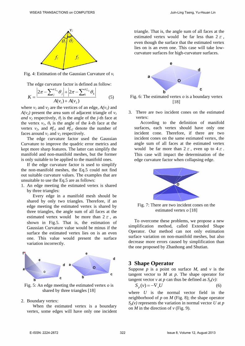
Fig. 4: Estimation of the Gaussian Curvature of vi

The edge curvature factor is defined as follow:

)()(

22

21

##21

vAvAK

vv f

k k

f

j j

(5)

where v1 and v2 are the vertices of an edge, A(v1) and

A(v2) present the area sum of adjacent triangle of v1

and v2 respectively, θj is the angle of the j-th face at

the vertex v1, θk is the angle of the k-th face at the

vertex v2, and #fv1 and #fv2 denote the number of

faces around v1 and v2 respectively.

The edge curvature factor used the Gaussian

Curvature to improve the quadric error metrics and

kept more sharp features. The latter can simplify the

manifold and non-manifold meshes, but the former

is only suitable to be applied to the manifold ones.

If the edge curvature factor is used to simplify

the non-manifold meshes, the Eq.5 could not find

out suitable curvature values. The examples that are

unsuitable to use the Eq.5 are as follows:

1. An edge meeting the estimated vertex is shared

by three triangles:

Every edge in a manifold mesh should be

shared by only two triangles. Therefore, if an

edge meeting the estimated vertex is shared by

three triangles, the angle sum of all faces at the

estimated vertex would be more than 2π, as

shown in Fig.5. That is, the estimation of

Gaussian Curvature value would be minus if the

surface the estimated vertex lies on is an even

one. This value would present the surface

variation incorrectly.

Fig. 5: An edge meeting the estimated vertex o is

shared by three triangles [18]

2. Boundary vertex:

When the estimated vertex is a boundary

vertex, some edges will have only one incident

triangle. That is, the angle sum of all faces at the

estimated vertex would be far less than 2π ,

even though the surface that the estimated vertex

lies on is an even one. This case will take low-

curvature surfaces for high-curvature surfaces.

Fig. 6: The estimated vertex o is a boundary vertex

[18]

3. There are two incident cones on the estimated

vertex:

According to the definition of manifold

surfaces, each vertex should have only one

incident cone. Therefore, if there are two

incident cones on the same estimated vertex, the

angle sum of all faces at the estimated vertex

would be far more than 2π, even up to 4π.

This case will impact the determination of the

edge curvature factor when collapsing edge.

Fig. 7: There are two incident cones on the

estimated vertex o [18]

To overcome these problems, we propose a new

simplification method, called Extended Shape

Operator. Our method can not only estimation

surface variation on non-manifold meshes, but also

decrease more errors caused by simplification than

the one proposed by Zhanhong and Shutian.

3 Shape Operator Suppose p is a point on surface M, and v is the

tangent vector to M at p. The shape operator for

tangent vector v at p can thus be defined as Sp(v):

UvS vp )( (6)

where U is the normal vector field in the

neighborhood of p on M (Fig. 8); the shape operator

Sp(v) represents the variation in normal vector U at p

on M in the direction of v (Fig. 9).



Fig. 8: Normal vector field on surface M [2]

Fig. 9: Shape operator estimation for tangent vector

v at point p on surface M [2]

The shape operator refers to the variation in the

normal vector field in the direction of vector v at

point p on surface M. To calculate surface changes

in the neighborhood of p, Jong et al. [2, 13] used

variations in the normal vectors of p and its

neighboring points for estimation. Suppose the k

neighboring points of p are p1, p2, p3,…, and pk, and

the tangent vectors of p toward each neighboring

point are t1, t2, t3,…, and tk . Calculations from Eq. 6

provide the shape operators Sp(t1), Sp(t2), Sp(t3),…,

and Sp(tk) at p in the directions of t1, t2, t3,…, and tk.

Integrating all of the shape operators enables the

derivation of the following formula to estimate

variations in the surface surrounding p:

k

i i

k

i i

p

pp

pUpUS

1

1)()(

(7)

Fig. 10: Shape operators of point p using the tangent

vectors to each neighboring point to estimate local

surface variation

In practice, this is based on a tangent plane.

Suppose there is a tangent plane TPp at point p; the

projections of 1pp , 2pp , 3pp ,…, and kpp are

used to obtain the required tangent vectors t1, t2,

t3,…, and tk, which are then employed to derive the

shape operators at p in the direction of said vectors.

Using the shape operators enables the estimation of

overall variations in the local surface area.

Examples of implementation results are presented in

Fig. 11.

Fig. 11: Surface variation estimation; green

represents areas of minor variation, whereas red

indicates areas of major variation

The shape operator is used to estimate surface

variations by neighboring vertices on 3D models

prior to vertex-pair contraction in order to reduce

the error caused by simplification. Nevertheless, for

the simplification of models at lower resolutions,

considering only the first ring of neighboring

vertices is far from adequate. When simplification

results in a smaller number of triangles, the

simplified vertices cover a larger area. For this

reason, the range under consideration should also be

extended. This study proposes the Extended Shape

Operator to reduce error resulting from the

simplification to the fewest possible number of

triangles.

4 Extended Shape Operator

4.1 Analyzing the Impact Area of Simplified

Vertices To analyze the impact areas of simplified vertices,

we perform an experiment to calculate the moving

distance of each simplified vertex. This experiment

uses four models, including a cow, a dragon, a

femur and an isis. The half edge collapse [1] is

adopted to record the moving path of each

simplified vertex in the simplification process

because it will allow the vertex moving to the other

one in the collapsing edge.

high

low



In this experiment, we simplify the above models

into five different resolutions, include 40%, 30%,

20%, 10% and 5%. The experimental results are

shown in Tables 1 to 4. In these tables, the moving

length presents the moving times of vertex when it

is simplified. Taking the cow model (Table 1) as an

example, when the cow model is simplified into

forty percent of triangles, 1315 vertices are moved

one time, 387 vertices are moved two times, 38

vertices are move three times, 2 vertices are moved

more than 3 times, and 1162 vertices still stay at

their original positions.

Table 1: Moving length analysis of simplified vertex

(cow model; the number of vertices =2904)

SP 5% 10% 20% 30% 40%

ML The number of vertices

0 148 293 583 873 1162

1 651 971 1272 1359 1315

2 1021 1025 810 566 387

3 726 490 218 102 38

>3 358 125 21 4 2

AML 2.19 1.72 1.25 0.97 0.76

SP : simplification percentage

ML : moving length

AML : average moving length


(dragon model; the number of vertices=25418)

SP 5% 10% 20% 30% 40%


0 1277 2546 5084 7622 10160

1 6095 9147 12308 13320 12906

2 9691 9617 6862 4026 2036

3 6327 3501 922 226 92

>3 2028 607 242 224 224

AML 2.11 1.66 1.21 0.94 0.75


(femur model; the number of vertices=76794)

SP 5% 10% 20% 30% 40%


0 3873 7715 15397 23074 30748

1 17366 26040 34774 37525 36496

2 28309 29082 22278 14739 9025

3 20201 12088 4108 1421 519

>3 7045 1869 237 35 6

AML 2.13 1.67 1.21 0.93 0.73


(isis model; the number of vertices=100002)

SP 5% 10% 20% 30% 40%


0 5002 10002 20002 30002 40002

1 23494 35670 48645 52994 51925

2 38204 38757 27985 16393 7990

3 25715 14100 3322 612 85

>3 7587 1473 48 1 0

AML 2.08 1.61 1.15 0.88 0.68

According to the experimental results, the

average moving lengths are less than three, even if

the models are simplified into only five percent of

the number of triangles. Additionally, the percent of

the number of vertices that the moving lengths are

less than or equal three are almost over ninety

percent, as shown in Table 5. Therefore, we extend

the range from one ring to three rings for the

estimation of surface variation.

Table 5: The percent of the number of vertices with

moving length<=3 in different simplification

percentage

SP 5% 10% 20% 30% 40%

Models The percent of the number of vertices

with moving length<=3 (%)

cow 87.67 95.70 99.28 99.86 99.93

dragon 92.02 97.61 99.05 99.12 99.12

femur 90.83 97.57 99.69 99.95 99.99

isis 92.41 98.53 99.95 100 100

SP: simplification percentage

4.2 The Proposed Algorithm Shape operators generally only consider the

neighboring points of p, as shown in Fig. 12(a). To

obtain a low-resolution model of higher quality after

simplification, this study expanded the estimation

range to N rings of neighboring points. As shown in

Fig. 12(b), p1,1, p1,2, p1,3,…, and p1,M1 represent the

first ring of points neighboring p; p2,1, p2,2, p2,3,…,

and p2,M2 are the second ring of points neighboring p,

and p3,1, p3,2, p3,3,…, and p3,M3 comprise the third

ring of points neighboring p. Likewise, we can

define the Nth ring of points neighboring p as pN,1,

pN,2, pN,3,…, and pN,MN. As simplification of the



model proceeds, the number of triangles in the mesh

of the model dwindles. In other words, the impact

range of each vertex expands and the data that each

vertex encompasses increases as well. For example,

as shown in Fig. 13, point p is a vertex on a dragon

model; during the first simplification, the area that p

influences lies within the first ring of neighboring

points. During the second simplification, the area

that p may influence extends to the second ring of

neighboring points, and so forth. After several

iterations, the area influenced by each vertex

expands. Therefore, we extended the estimation

range of the shape operator to the Nth ring. The

formula to estimate the N-rings shape operator of

the area where p is located is:

N

j

M

i ij

N

j

M

i ijN

pj

j

pp

pUpU

1 1 ,

1 1 , )()(S (8)

where

N : the number of rings;

pj,i : the ith point neighboring p in the jth ring;

U(pj,i) : the normal vector at point pj,i;

Mj: the number of points neighboring p in the jth

ring.

The variations in the normal vectors of each ring are:

The first ring :

1

1 ,1 )()(M

i i pUpU

The second ring :

2

1 ,2 )()(M

i i pUpU

The third ring :

3

1 ,3 )()(M

i i pUpU

:

:

:

The Nth ring :

NM

i iN pUpU1 , )()(

(a) the first ring

(b) the first to third rings

Fig. 12: N rings centered at p (N=1…3)

Basically, the Extended Shape Operator

simplification is an improved algorithm for the

QEM simplification. Prior to estimating the QEM,

we first find out the N-rings shape operator N

pS for

each point p, calculate the surface variation within

the range of N rings neighboring p, and then use N

pS as the weight value to improve the QEM. The

Extended Shape Operator can reduce the error

caused by simplification when the model is

simplified to lower resolutions.

Fig. 13: The N-rings neighboring points of point p

p

p2 p3

p4 p5

p1

p1,1

p p1,5

p1,4

p1,3

p1,2 p2,1

p2,2 p2,3 p2,4

p2,5 p3,1

p3,2

p3,3 p3,4

p3,M3

p3,5 p3,6

p

p1,1 p1,2

p1,3

p1,4 p1,5

p1,6 p1,7

p2,1 p2,2 p2,3

p2,M2-1 p2,M2

p3,1 p3,2

p3,3

p3,M3-1 p3,M3

The first ring

The second ring

The third ring



The primary calculation steps of the proposed

simplification approach are as follows:

1. Calculate the shape operator of each vertex {(p1,1,

p1,2,…, p1,M1), (p2,1, p2,2,…, p2,M2),…, (pN,1, pN,2,…,

pN,MN)}. Using Eq. (8), estimate the N-rings shape

operator N

pS of p and change the QEM

estimation formula to:

f

N

p KSpQ )( (9)

where

f is the plane encompassing the triangles

with p as a vertex;

Kf represents the 44 matrix of plane f.

2. Select each qualifying vertex pair (v1,v2), and

calculate the minimum error resulting from

simplification.

3. Select the vertex pair (v1,v2) with the minimum

error for simplification.

4. Contract vertex pair (v1,v2) into v , and calculate

the QEM of v using Q=(Q1+Q2), where Q1 and

Q2 are the QEMs of v1 and v2 , respectively.

5. Update the information regarding the points

neighboring v1 and v2.

6. Repeat the steps above until the designated

number of triangles is reached.

5 Experimental Results This study implemented an experiment with three

rings to verify the Extended Shape Operator (ESO)

simplification method proposed in this study. We

conducted comparisons with the Curvature Factor. Four models were employed for the simplification

experiment: a cow, a dragon, a femur, and an isis.

The number of vertices and triangles are shown in

Table 6.

Table 6: Information of Experimental Models

Model Vertices Triangles

Cow 2904 5804

Dragon 25419 50761

Femur 76794 153322

Isis 100002 200000

This study employed Hausdorff Distance

implemented in Metro [11] to measure the error

caused by simplification and understand the

variations in the shapes of the models before and

after simplification. Errors occurring in the

Curvature Factor (CF) [14] were also measured.

The results of the four methods were then compared.

The results of the experiment show that the

proposed method is more effective than the

Curvature Factor method in reducing error. In the

cow model, for example, the number of triangles

was reduced from 5804 to 2321, 1741, 1160, 580

and 290. The Curvature Factor resulted in errors of

0.02146, 0.02552, 0.02985, 0.02948, and 0.04829,

respectively, whereas the proposed method only

caused errors of 0.00415, 0.00497, 0.00636,

0.01126, and 0.01813. This accounted for

improvements of 80.68%, 80.53%, 78.71%, 61.81%,

and 62.46% compared to the Curvature Factor,

respectively, as shown in Table 7, Fig.14 and Fig.21.

Table 7: Hausdorff Distance Comparison

(unit : 10−2) – cow model

SP Triangles CF ESO IR

40% 2321 2.146 0.415 80.68%

30% 1741 2.552 0.497 80.53%

20% 1160 2.985 0.636 78.71%

10% 580 2.948 1.126 61.81%

5% 290 4.829 1.813 62.46%

SP : Simplification Percentage

IR : Improvement Rate

Fig. 14: Error measurement for cow model

Besides taking the cow model for verification,

the dragon, femur and isis models are taken for

experimental testing. In the dragon model, the

original model contains 25419 vertices and 50761

triangles. Figure 22 shows the simplification results.

Table 8 and Fig. 15 compare the error

measurements with the Curvature Factor and the

proposed method; the table shows that the proposed

method can achieve an 45.95–81.08% error

reduction. In the femur and isis models, the original

models contain 153322 and 200000 triangles

respectively. Figures 23 and 24 show the

simplification results of the femur and isis models.

Tables 9, 10 and Figs. 16, 17 compare the error

measurements with the Curvature Factor and the



proposed method; the tables show that the proposed

method can achieve 88.29–98.66% and 71.95–

84.08% error reductions for the simplifications of

the femur and isis models respectively.


(unit : 10−3) – dragon model


40% 20304 2.622 0.496 81.08%

30% 15228 3.517 0.651 81.49%

20% 10152 4.055 1.002 75.29%

10% 5076 5.272 1.369 74.03%

5% 2538 5.384 2.910 45.95%

SP : Simplification Percentage

IR : Improvement Rate

Fig. 15: Error measurement for dragon model


(unit : 10−3) – femur model


40% 61328 17.206 0.231 98.66%

30% 45996 17.210 0.414 97.59%

20% 30664 17.264 0.649 96.24%

10% 15332 17.258 0.648 96.25%

5% 7666 17.202 2.015 88.29%

Fig. 16: Error measurement for femur model


(unit : 10−3) –isis model


40% 80000 1.583 0.252 84.08%

30% 60000 1.986 0.408 79.46%

20% 40000 2.583 0.369 85.71%

10% 20000 2.830 0.683 75.87%

5% 10000 3.540 0.993 71.95%

Fig. 17: Error measurement for isis model

In terms of feature preservation, Fig. 18 shows

the comparison results of the QEM, the CF and the

proposed method for simplifying the cow model

into one with 580 triangles. Apparently, regarding

the cow horn features, the CF can preserve the

model features better than the QEM. However, the

former also impact on the outline of cow neck. The

proposed method can not only preserve the outline

of cow horn, but also retain the shape of cow neck.

In addition, Fig. 19 shows the comparison results of

the CF and the proposed method for simplifying the

dragon model into one with 5076 triangles. The

figure shows that our method can retain more teeth

and eye features of the dragon model than the CF.

(a) original model

(b) QEM (c) CF (d) ESO

Fig. 18: Comparison of the features of cow horns

and neck (580 triangles).



(a) original model (b) CF (c) ESO

Fig. 19: Comparison of the features of dragon teeth

(5076 triangles).

Moreover, the Curvature Factor method will also

destroy the features of hole easily due to the

improper angle estimation on non-manifold surfaces.

Taking the femur model as an example, although the

boundary vertices by the hole are not on a high-

curvature surface, the triangles meeting these

vertices are still destroyed easily due to being taken

for on a high-curvature surface.

(a) original model

(b) CF (c) ESO

Fig. 20: Comparison of the hole features of femur

(7666 triangles).

6 Conclusions The primary objective of 3D model simplification is

to maintain the characteristic contours of the model

despite reducing the resolution. The Curvature

Factor method employs the Gaussian Curvature to

preserve features of simplified models. However, it

can only be used to simplify manifold models. To

preserve the features of non-manifold model, this

study proposes a novel method, called the Extended

Shape Operator. The proposed method uses three-

rings Shape Operator to estimate the surface

variation and preserves more features than the

Curvature Factor. Experimental results show that

the Extended Shape Operator can also reduce the

error caused by simplification.

References:

[1] M. Garland and P. S. Heckbert, Surface

simplification using quadric error metrics,

SIGGRAPH 97 Conference Proceedings, 1997,

pp. 209-216.

[2] B. S. Jong, J. L. Tseng, W. H. Yang and T. W.

Lin, Extracting Features and Simplifying

Surfaces using Shape Operator, International

Conference on Information, Communications

and Signal Processing, 2005, pp.1025-1029.

[3] J. L. Tseng, Shape-based simplification for 3d

animation models using shape operator

sequences, 4th NAUN/WSEAS International

Conference on Communications and

Information Technology, Corfu Island, Greece,

July 22-25, 2010, pp.90-95.

[4] P. F. Lee and C. P. Huang , The DSO Feature

Based Point Cloud Simplification, 2011 Eighth

International Conference on Computer

Graphics, Imaging and Visualization, 2011,

pp.1-6.

[5] Z. Y. Yang, S. W. Xu and W. Y. Wu, A Mesh

Simplification Algorithm for Keeping Local

Features with Mesh Segmentation, 2010

International Conference on Mechanic

Automation and Control Engineering, 2010,

pp.5487-5490.

[6] Y. Li, Q. Zhu, A New Mesh Simplification

Algorithm Based on Quadric Error Metrics,

International Conference on Advanced

Computer Theory and Engineering, 2008,

pp.528-532.

[7] A. Gu´eziec, Surface simplification with

variable tolerance, Second Annual Intl. Symp.

on Medical Robotics and Computer Assisted

Surgery (MRCAS ’95), 1995, pp.132–139.

[8] H. Bernd , A Data Reduction Scheme for

Triangulated Surfaces, Computer Aided

Geometric Design, Vol.11, 1994, pp.197-214.

[9] J. Rossignac and P. Borrel , Multi- resolution

3D approximations for rendering complex

scenes , Modeling in Computer Graphics:

Methods and Applications, 1993, pp. 455–465.

[10] T. S. Gieng, B. Hamann, K. I. Joy, Gregory L.

Schussman, and Issac J. Trotts, Constructing

hierarchies for triangle meshes , IEEE

Transactions on Visualization and Computer

Graphics vol.4, no.2 , 1998, pp.145–161.

[11] P. Cignoni, C. Rocchini, R. Scopigno, Metro:

measuring error on simplified surfaces,

Computer Graphics Forum, Vol.17, No.2,

1998, pp.167-174.

boundary vertex



[12] V. Ungvichian and P. Kanongchaiyos, Mesh

Simplification Method Using Principal

Curvatures and Directions, Computer Modeling

in Engineering & Sciences, Vol.77, No.4, 2011,

pp.201-220.

[13] B. S. Jong, J. L. Tseng and W. H. Yang, An

Efficient and Low-Error Mesh Simplification

Method Based on Torsion Detection, The

Visual Computer, Vol.22, No.1, Jan. 2006,

pp.56-67.

[14] T. Zhanhong and Y. Shutian, A Mesh

Simplification Algorithm Based on Curvature

Factor of Collapsing Edge, 2nd IEEE

International Workshop on Database

Technology and Applications, 2010, pp.1-3.

[15] M. H. Mousa and M. K. Hussein, Adaptive

visualization of 3D meshes using localized

triangular strips, WSEAS Transactions on

Computers, Vol.11, No.4, 2012, pp.101-110.

[16] H. U. Khan, Replica Technique for Geometric

Modelling, WSEAS Transactions on

Information Science and Applications, Vol.6,

No.6, 2009, pp.1071-1081.

[17] C. D. Ruberto, M. Gaviano, A. Morgera, Shape

Matching by Curve Modelling and Alignment,

WSEAS Transactions on Information Science

and Applications, Vol.6, No.4, 2009, pp.567-

578.

[18] M. Chena, B. Tub, B. Lu, Triangulated

manifold meshing method preserving

molecular surface topology, Journal of

Molecular Graphics and Modelling, Vol.38,

2012, pp. 411-418.

[19] M. Meyer, M. Desbrun, P. Schröder , A.H. Barr,

Discrete Differential-Geometry Operators for

Triangulated 2-Manifolds, Proceedings of

VisMath, 2002.

(a) 5804 triangles (original model) (b) 2321 triangles (40%) (c) 1741 triangles (30%)

(d) 1160 triangles (20%) (e) 580 triangles (10%) (f) 290 triangles (5%)

Fig. 21: Simplification results of the cow model using the ESO.

(a) 50761 triangles (original model) (b) 20304 triangles (40%) (c) 15228 triangles (30%)



(d) 10152 triangles (20%) (e) 5076 triangles (10%) (f) 2538 triangles (5%)

Fig. 22: Simplification results of the dragon model using the ESO.

(a) (b) (c) (d) (e) (f)

Fig. 23: Simplification results of the femur model using the ESO. (a) 153322 triangles (original model), (b)

61328 triangles, (c) 45996 triangles, (d) 30664 triangles, (e) 15332 triangles, (f) 7666 triangles.

(a) (b) (c) (d) (e) (f)

Fig. 24: Simplification results of the isis model using the ESO. (a) 200000 triangles (original model), (b) 80000

triangles, (c) 60000 triangles, (d) 40000 triangles, (e) 20000 triangles, (f) 10000 triangles.



3d surface simplification based on extended shape operator

Documents