Transport in potentials random in space and time: From Anderson

localization to super-ballistic motion

• Yevgeny Krivolapov, Michael Wilkinson, SF

• Liad Levy, Moti Segev

Physics of Noise

• Is noise uninteresting?

• Rules of noise?

• Universality classes of noisy behavior?

• Random can be systematic!!

• Central limit theorem

• Statistical Mechanics!!

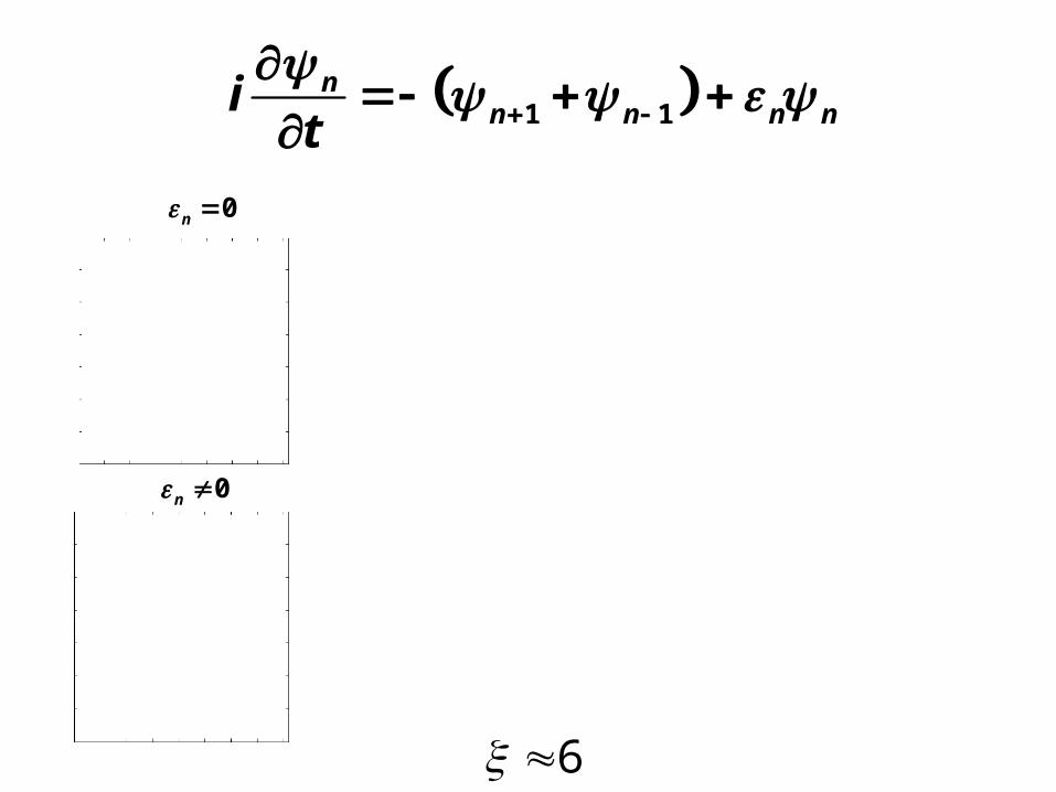
0n

0n

1 1n

n n n nit

6

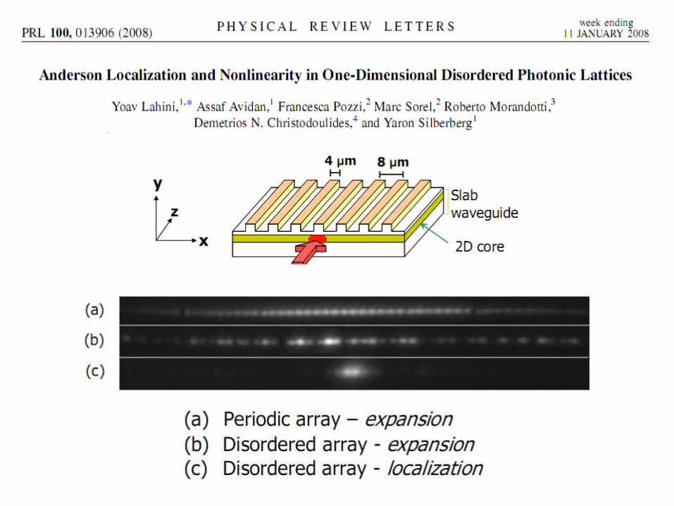
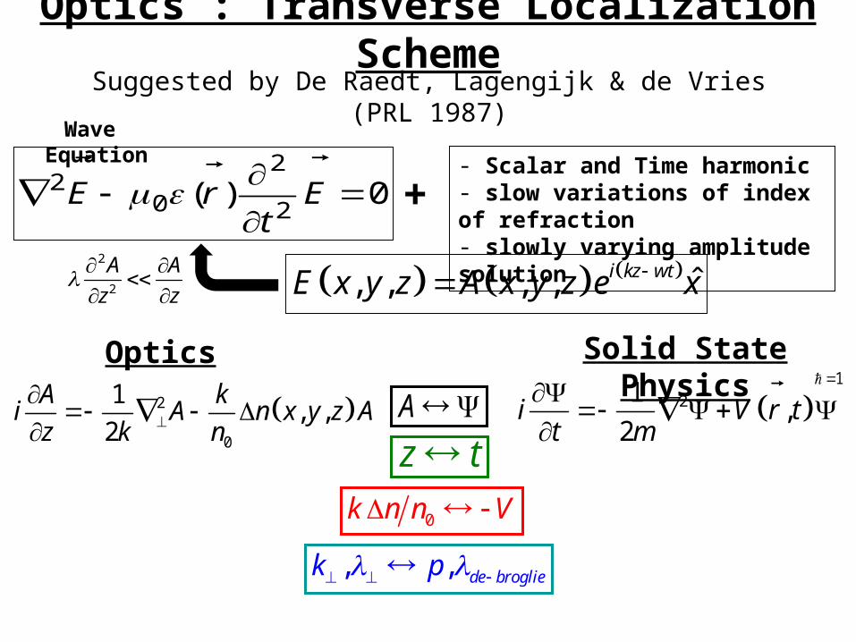
Optics : Transverse Localization Scheme

ˆ, , , , i kz wtE x y z A x y z e x

2

0

1, ,

2

A ki A n x y z Az k n

21

,2

i V r tt m

Optics Solid State Physics

0k n n V

0)(2

2

02

E

trE

Wave Equation

+- Scalar and Time harmonic- slow variations of index of refraction- slowly varying amplitude solution

z tA

1

2

2

A A

z z

, , de brogliek p

Suggested by De Raedt, Lagengijk & de Vries (PRL 1987)

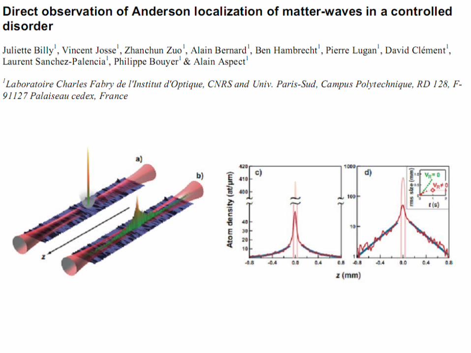
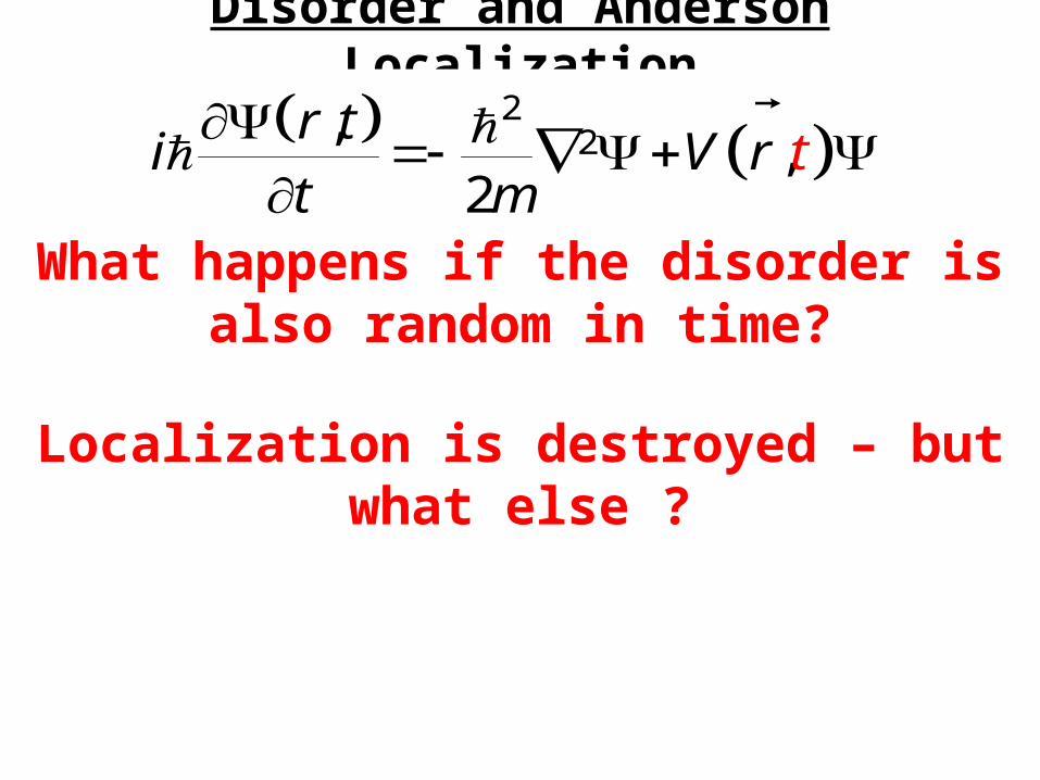
Disorder and Anderson Localization

Disordered Potential:

Localized StatesTypical scale ξ

The wave remains confined in some region of the potentialPhilip W. Anderson, 1958 (Nobel Prize 1977)

- Localization Length

Periodic Potential:

Bloch waves (extended states)

xV

A wave packet propagating freely through the medium exhibits

Ballistic Transport/Diffraction

2

2,

2

r ti V r

t m

2

2,,

2

r ti

t mtV r

What happens if the disorder is also random in time?

Localization is destroyed – but what else ?

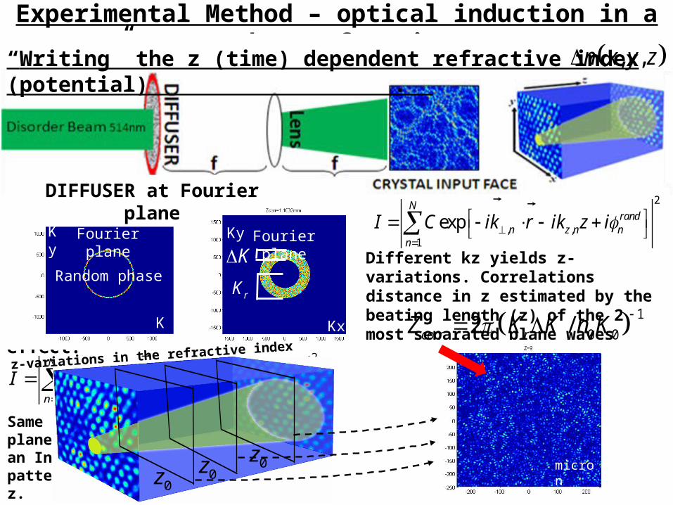
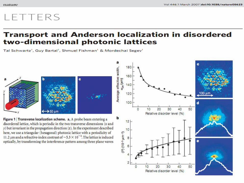
Experimental Method – optical induction in a photorefractive We utilize the photorefractive screening effect inside a 10mm-long SBN:60 crystal, in which separation of optically-excited charges (electrons) creates a varying electric space-charge field, which in turn induces a local change in the refractive index via the electro-optic effect.

Ensemble average on many disorder realizations

Fourier plane

Kx

Ky

Random phase

2

,1

expN

randn z n

n

I C ik r ik z i

DIFFUSER at Fourier plane

z

“Writing” the z (time) dependent refractive index (potential) . , ,n x y z

1

0 02 /corr rZ K K n K

Same kz for all plane waves yields an Interference pattern constant in z.

rK

KFourier plane

Kx

Ky

Different kz yields z- variations. Correlations distance in z estimated by the beating length (z) of the 2 most separated plane waves

2

, ,1

expN

randn z n n

n

I C ik r ik z i

z-variations in the refractive index

0z0z

0z micron

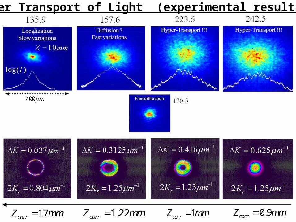
Hyper Transport of Light (experimental results)

17corrZ mm 1.22corrZ mm 1corrZ mm 0.9corrZ mm

400 m

High momentum

h

p

Semi-classical

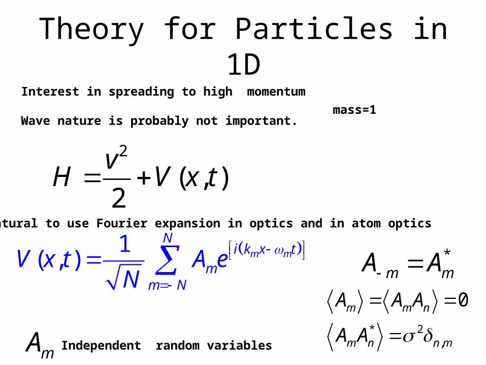
Theory for Particles in 1DInterest in spreading to high momentum

Wave nature is probably not important.

2

( , )2

vH V x t

Natural to use Fourier expansion in optics and in atom optics

1( , ) m m

Ni k x t

mm N

V x t A eN

*m mA A

* 2,

0m m n

m n n m

A A A

A A

mA Independent random variables

mass=1

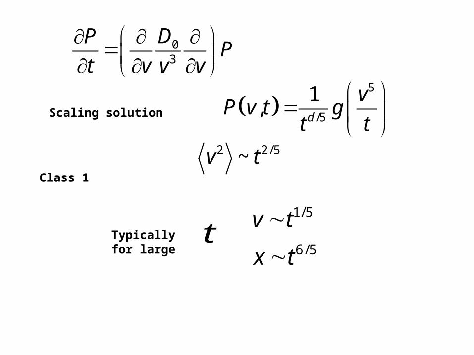
03

DPP

t v v v

2 2/5~v t

5

/5

1,

d

vP v t g

t t

Scaling solution

Typically for large

t1/5

6/5

v t

x t

Class 1

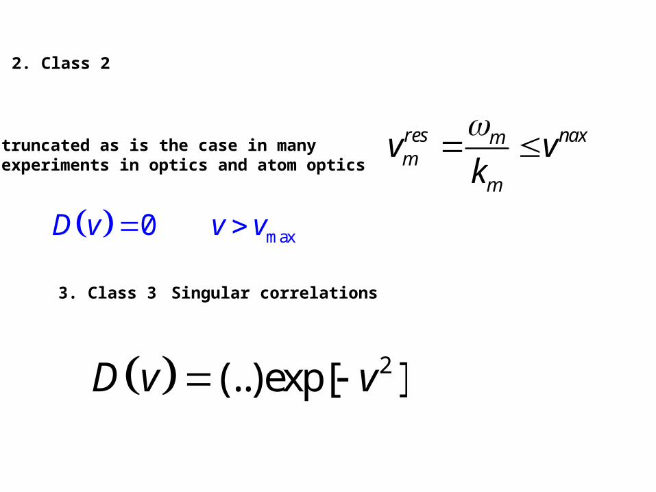
2. Class 2

max0D v v v

res naxmm

m

v vk

truncated as is the case in many

experiments in optics and atom optics

3. Class 3 Singular correlations

2(..)exp[ ]D v v

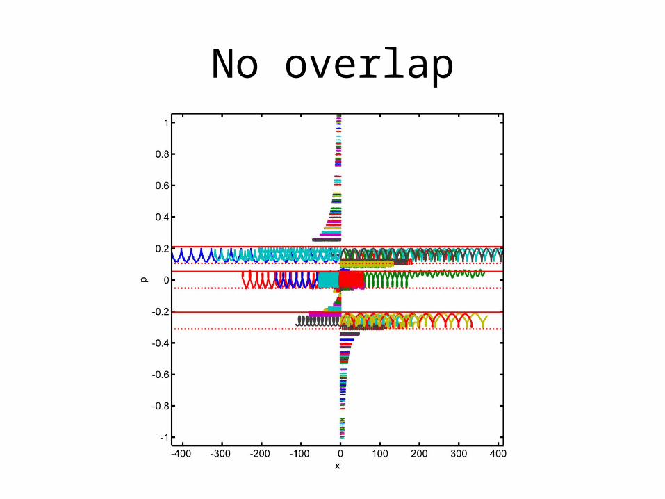
No overlap

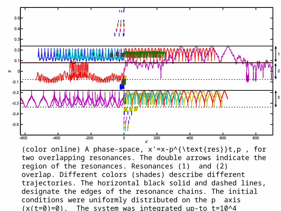
(color online) A phase-space, x'=x-p^{\text{res}}t,p , for two overlapping resonances. The double arrows indicate the region of the resonances. Resonances (1) and (2) overlap. Different colors (shades) describe different trajectories. The horizontal black solid and dashed lines, designate the edges of the resonance chains. The initial conditions were uniformly distributed on the p axis (x(t=0)=0). The system was integrated up-to t=10^4 (dimensionless variables).

0 1 2 3 4 5 6 7 8 9 10

x 106

0

0.5

1

1.5

2

2.5

3

3.5

4x 10

-3

t

<p

2 >

N=300N=200N=100Theory

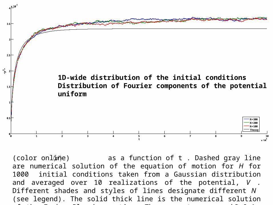
(color online) as a function of t . Dashed gray line are numerical solution of the equation of motion for H for 1000 initial conditions taken from a Gaussian distribution and averaged over 10 realizations of the potential, V . Different shades and styles of lines designate different N (see legend). The solid thick line is the numerical solution of the Focker-Planck equation. The parameters are, kR=0.1 and A=1e-4.

2p

1D-wide distribution of the initial conditionsDistribution of Fourier components of the potentialuniform

0 0.5 1 1.5 2 2.5 3

x 105

0.2

0.4

0.6

0.8

1

1.2

1.4

1.6

1.8

2

x 10-3

t

<p2 >

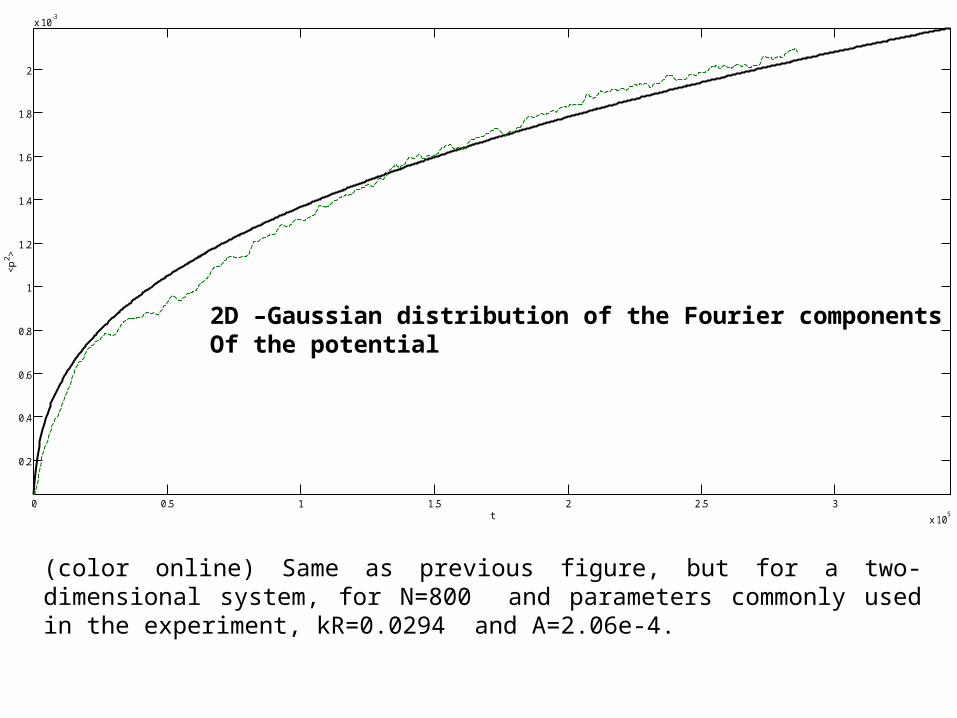
(color online) Same as previous figure, but for a two-dimensional system, for N=800 and parameters commonly used in the experiment, kR=0.0294 and A=2.06e-4.

2D –Gaussian distribution of the Fourier componentsOf the potential

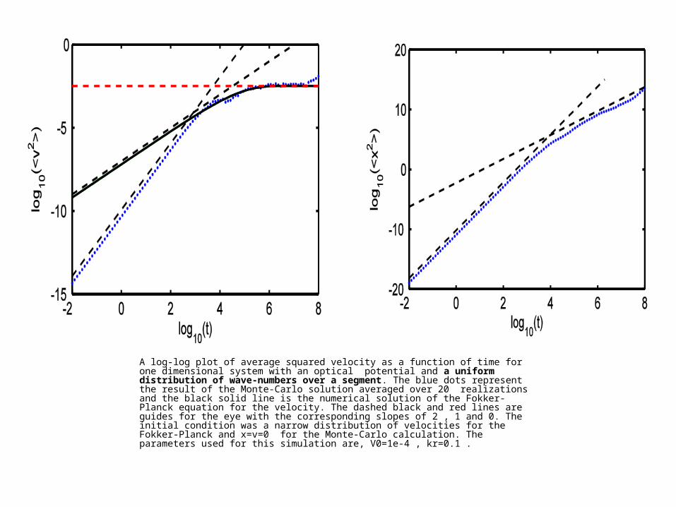
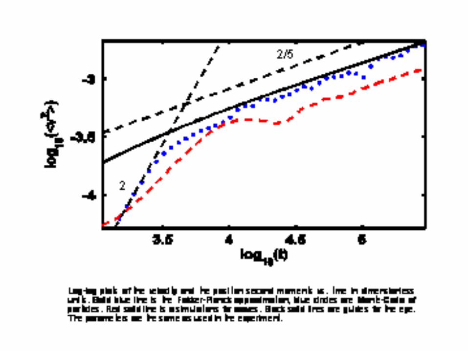
A log-log plot of average squared velocity as a function of time for one dimensional system with an optical potential and a uniform distribution of wave-numbers over a segment. The blue dots represent the result of the Monte-Carlo solution averaged over 20 realizations and the black solid line is the numerical solution of the Fokker-Planck equation for the velocity. The dashed black and red lines are guides for the eye with the corresponding slopes of 2 , 1 and 0. The initial condition was a narrow distribution of velocities for the Fokker-Planck and x=v=0 for the Monte-Carlo calculation. The parameters used for this simulation are, V0=1e-4 , kr=0.1 .

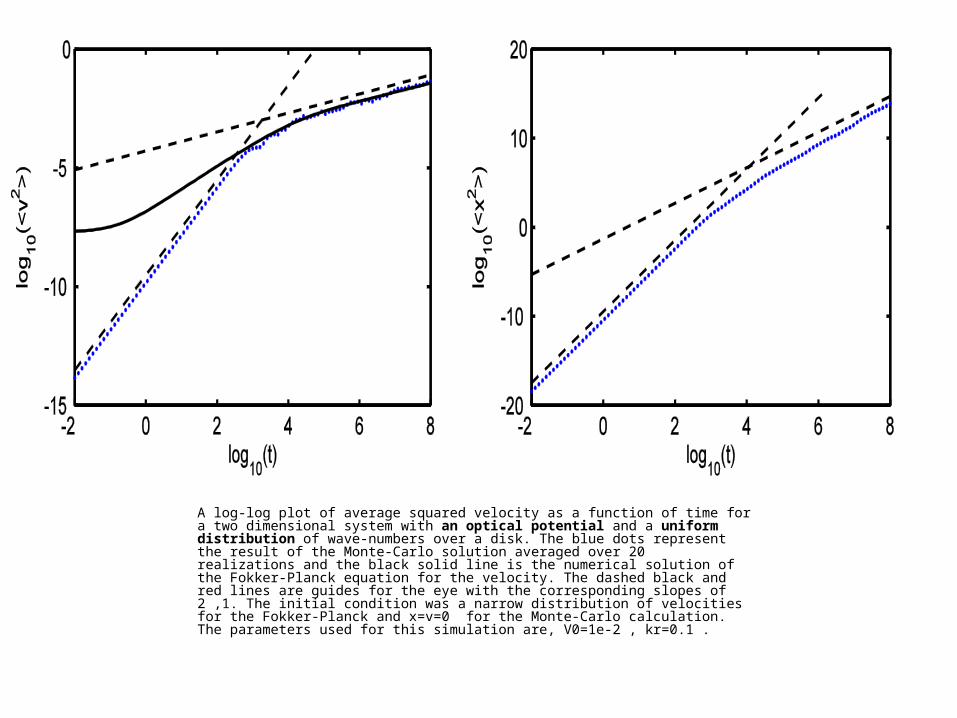
A log-log plot of average squared velocity as a function of time for a two dimensional system with an optical potential and a uniform distribution of wave-numbers over a disk. The blue dots represent the result of the Monte-Carlo solution averaged over 20 realizations and the black solid line is the numerical solution of the Fokker-Planck equation for the velocity. The dashed black and red lines are guides for the eye with the corresponding slopes of 2 ,1. The initial condition was a narrow distribution of velocities for the Fokker-Planck and x=v=0 for the Monte-Carlo calculation. The parameters used for this simulation are, V0=1e-2 , kr=0.1 .

For large momentum makes sense to use classical limit

h

p

Is there clash of limits problem??

summary

1. A formula for the diffusion coefficient in momentum in terms of the distribution function of the Fourier

components of the potential was developed. Natural

for potentials used in optics and atom optics 2. Classification into Universality classes

and Identification of new classes.

3. Identification of the uniform acceleration regime for short time.

Open problems

1. Identification of regimes that are not uniform acceleration where Fokker—Planck fails

2. An analytic theory for spreading in coordinate space.

3. Is there a regime of high momentum where waves spread in a way fundamentally different from particles?