x-ray fluorescence lab report - dashboard -...

X-Ray

Physics of XRF

XRF is a non destructive analytical technique that is used for elemental and chemical analysis.

X-Ray Fluorescence Spectroscopy is the emission of characteristic secondary x

material that has been excited by bombarding with

be used to investigate metals, glass, ceramics and building materials, and for research in

geochemistry, forensic science and archaeology.

are studying the analyses of major trace

when they interact with radiation.

radiation like x-rays, they become i

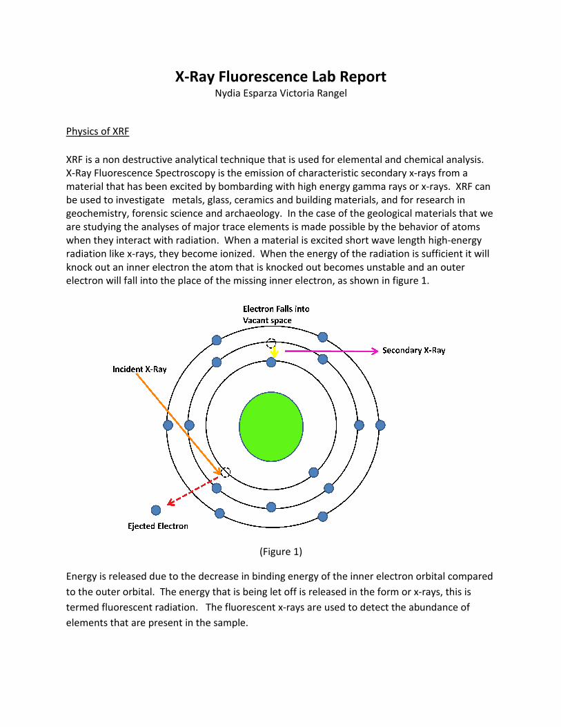
knock out an inner electron the atom

electron will fall into the place of the missing inner electron, as shown in figure 1.

Energy is released due to the decrease in binding energy of the

to the outer orbital. The energy that is

termed fluorescent radiation. The

elements that are present in the sample.

Ray Fluorescence Lab Report Nydia Esparza Victoria Rangel


Ray Fluorescence Spectroscopy is the emission of characteristic secondary x-rays from a

material that has been excited by bombarding with high energy gamma rays or x

metals, glass, ceramics and building materials, and for research in

geochemistry, forensic science and archaeology. In the case of the geological materials that we

analyses of major trace elements is made possible by the behavior of atoms

when they interact with radiation. When a material is excited short wave length high

rays, they become ionized. When the energy of the radiation is

atom that is knocked out becomes unstable and an

on will fall into the place of the missing inner electron, as shown in figure 1.

(Figure 1)

is released due to the decrease in binding energy of the inner electron orbital compared

The energy that is being let off is released in the form or x-

radiation. The fluorescent x-rays are used to detect the abundance of

elements that are present in the sample.


rays from a

high energy gamma rays or x-rays. XRF can

metals, glass, ceramics and building materials, and for research in

In the case of the geological materials that we

is made possible by the behavior of atoms

When a material is excited short wave length high-energy

onized. When the energy of the radiation is sufficient it will

unstable and an outer

on will fall into the place of the missing inner electron, as shown in figure 1.

inner electron orbital compared

-rays, this is

ays are used to detect the abundance of

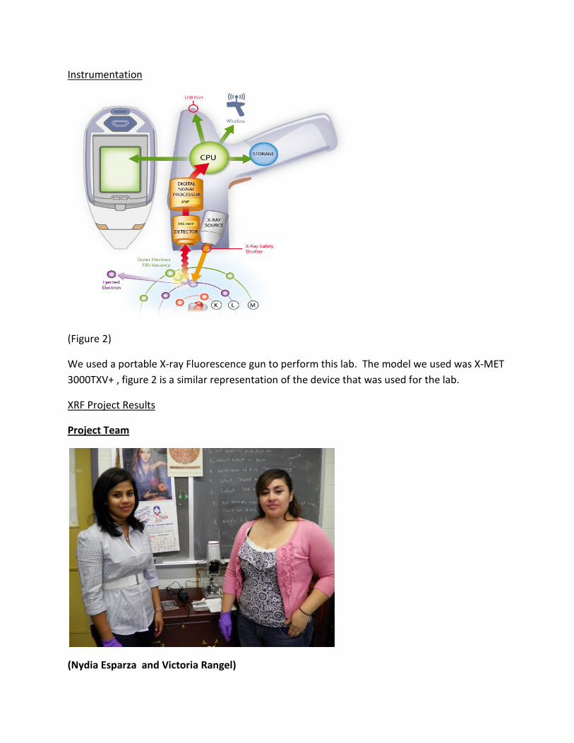
Instrumentation

(Figure 2)

We used a portable X-ray Fluorescence gun to perform this lab. The model we used was X-MET

3000TXV+ , figure 2 is a similar representation of the device that was used for the lab.

XRF Project Results

Project Team

(Nydia Esparza and Victoria Rangel)

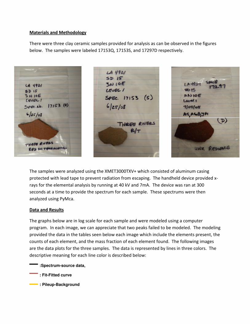
Materials and Methodology

There were three clay ceramic samples provided for analysis as can be observed in the figures

below. The samples were labeled 17153Q, 17153S, and 17297D respectively.

The samples were analyzed using the XMET3000TXV+ which consisted of aluminum casing

protected with lead tape to prevent radiation from escaping. The handheld device provided x-

rays for the elemental analysis by running at 40 kV and 7mA. The device was ran at 300

seconds at a time to provide the spectrum for each sample. These spectrums were then

analyzed using PyMca.

Data and Results

The graphs below are in log scale for each sample and were modeled using a computer

program. In each image, we can appreciate that two peaks failed to be modeled. The modeling

provided the data in the tables seen below each image which include the elements present, the

counts of each element, and the mass fraction of each element found. The following images

are the data plots for the three samples. The data is represented by lines in three colors. The

descriptive meaning for each line color is described below:

:Spectrum-source data,

: Fit-Fitted curve

: Pileup-Background

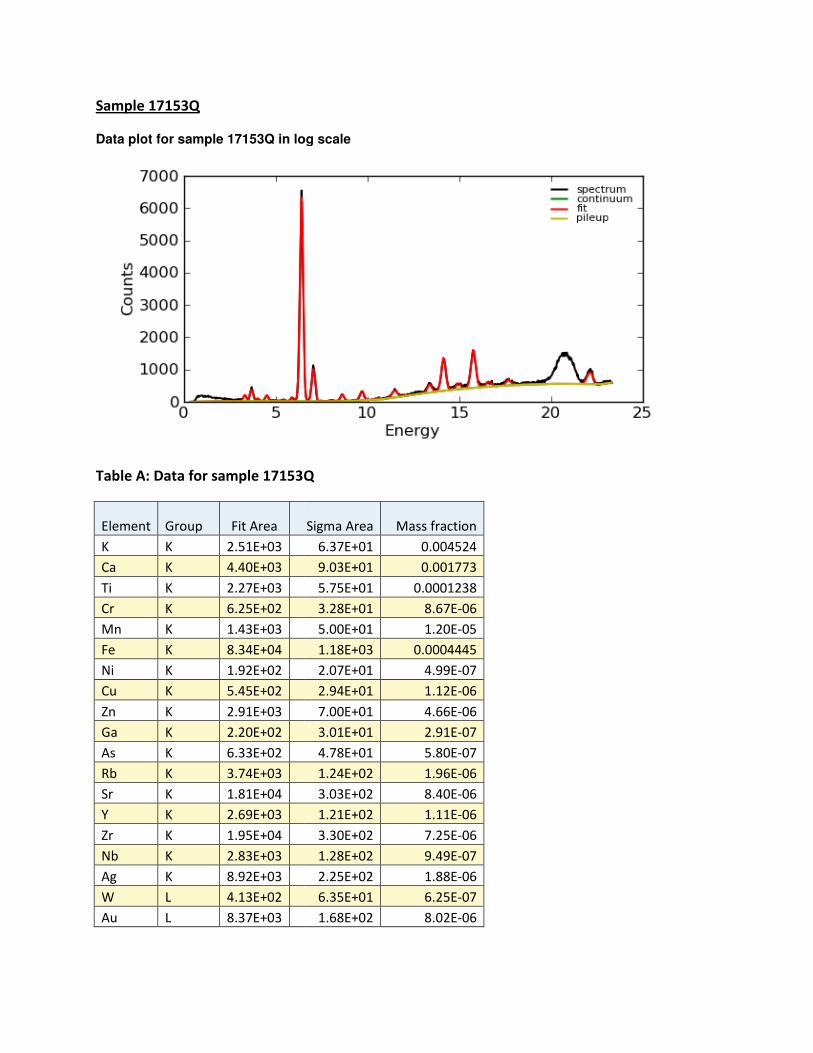
Sample 17153Q

Data plot for sample 17153Q in log scale

Table A: Data for sample 17153Q

Element Group Fit Area

K K 2.51E+03

Ca K 4.40E+03

Ti K 2.27E+03

Cr K 6.25E+02

Mn K 1.43E+03

Fe K 8.34E+04

Ni K 1.92E+02

Cu K 5.45E+02

Zn K 2.91E+03

Ga K 2.20E+02

As K 6.33E+02

Rb K 3.74E+03

Sr K 1.81E+04

Y K 2.69E+03

Zr K 1.95E+04

Nb K 2.83E+03

Ag K 8.92E+03

W L 4.13E+02

Au L 8.37E+03

in log scale

Table A: Data for sample 17153Q

Sigma Area Mass fraction

6.37E+01 0.004524

9.03E+01 0.001773

5.75E+01 0.0001238

3.28E+01 8.67E-06

5.00E+01 1.20E-05

1.18E+03 0.0004445

2.07E+01 4.99E-07

2.94E+01 1.12E-06

7.00E+01 4.66E-06

3.01E+01 2.91E-07

4.78E+01 5.80E-07

1.24E+02 1.96E-06

3.03E+02 8.40E-06

1.21E+02 1.11E-06

3.30E+02 7.25E-06

1.28E+02 9.49E-07

2.25E+02 1.88E-06

6.35E+01 6.25E-07

1.68E+02 8.02E-06

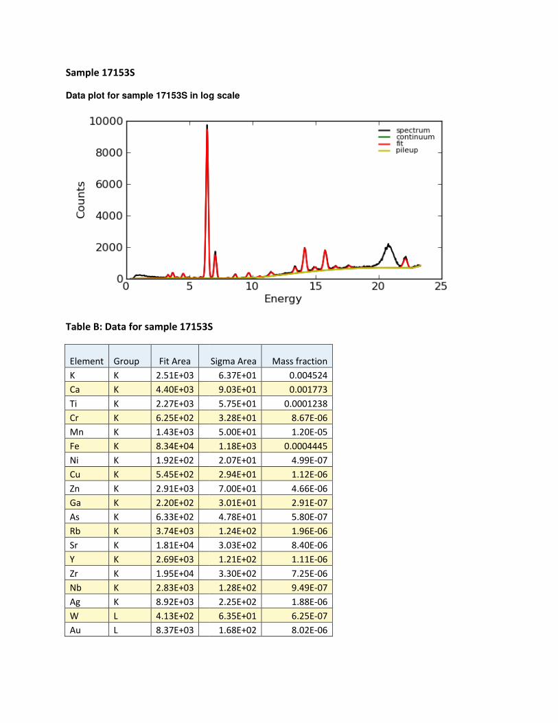
Sample 17153S

Data plot for sample 17153S in log scale

Table B: Data for sample 17153S

Element Group Fit Area

K K 2.51E+03

Ca K 4.40E+03

Ti K 2.27E+03

Cr K 6.25E+02

Mn K 1.43E+03

Fe K 8.34E+04

Ni K 1.92E+02

Cu K 5.45E+02

Zn K 2.91E+03

Ga K 2.20E+02

As K 6.33E+02

Rb K 3.74E+03

Sr K 1.81E+04

Y K 2.69E+03

Zr K 1.95E+04

Nb K 2.83E+03

Ag K 8.92E+03

W L 4.13E+02

Au L 8.37E+03

in log scale

: Data for sample 17153S


6.37E+01 0.004524

9.03E+01 0.001773

5.75E+01 0.0001238

3.28E+01 8.67E-06

5.00E+01 1.20E-05

1.18E+03 0.0004445

2.07E+01 4.99E-07

2.94E+01 1.12E-06

7.00E+01 4.66E-06

3.01E+01 2.91E-07

4.78E+01 5.80E-07

1.24E+02 1.96E-06

3.03E+02 8.40E-06

1.21E+02 1.11E-06

3.30E+02 7.25E-06

1.28E+02 9.49E-07

2.25E+02 1.88E-06

6.35E+01 6.25E-07

1.68E+02 8.02E-06

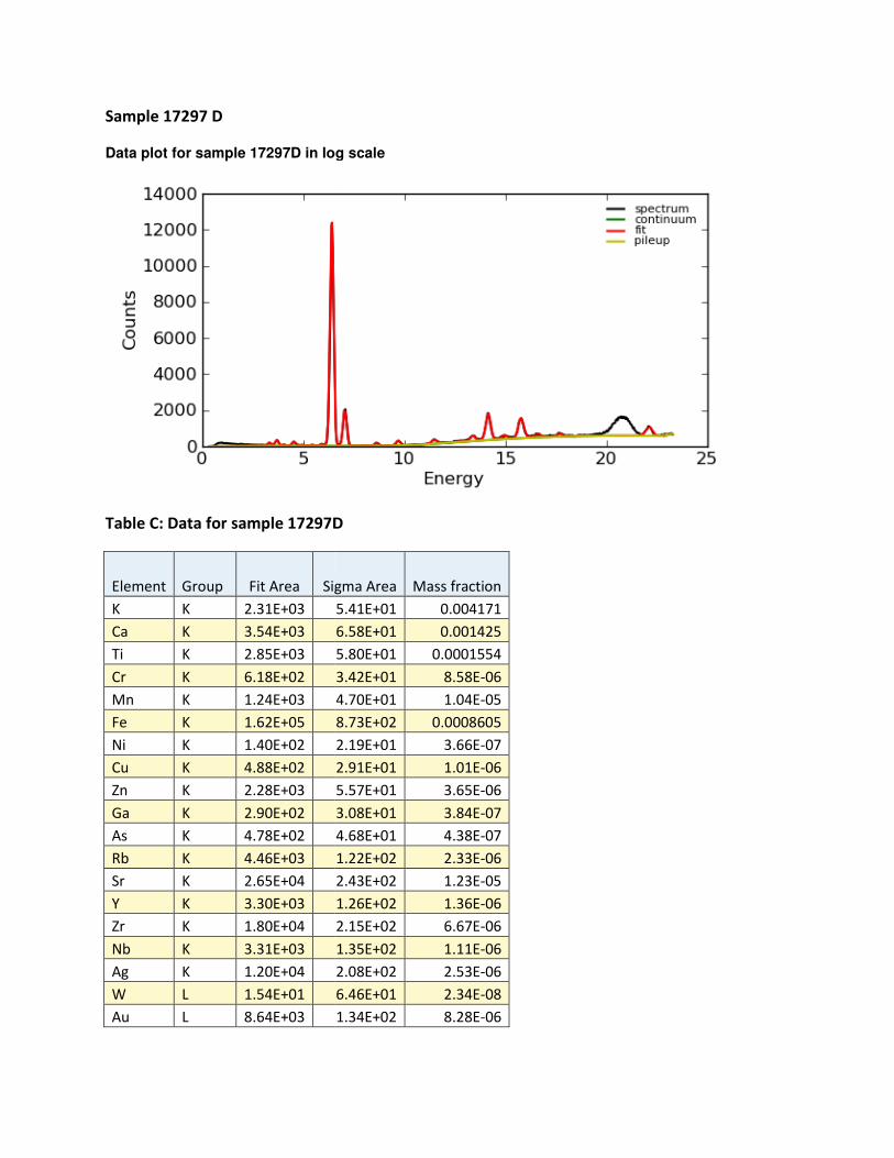
Sample 17297 D

Data plot for sample 17297D in log scale

Table C: Data for sample 17297D

Element Group Fit Area Sigma

K K 2.31E+03

Ca K 3.54E+03

Ti K 2.85E+03

Cr K 6.18E+02

Mn K 1.24E+03

Fe K 1.62E+05

Ni K 1.40E+02

Cu K 4.88E+02

Zn K 2.28E+03

Ga K 2.90E+02

As K 4.78E+02

Rb K 4.46E+03

Sr K 2.65E+04

Y K 3.30E+03

Zr K 1.80E+04

Nb K 3.31E+03

Ag K 1.20E+04

W L 1.54E+01

Au L 8.64E+03

in log scale

297D


5.41E+01 0.004171

6.58E+01 0.001425

5.80E+01 0.0001554

3.42E+01 8.58E-06

4.70E+01 1.04E-05

8.73E+02 0.0008605

2.19E+01 3.66E-07

2.91E+01 1.01E-06

5.57E+01 3.65E-06

3.08E+01 3.84E-07

4.68E+01 4.38E-07

1.22E+02 2.33E-06

2.43E+02 1.23E-05

1.26E+02 1.36E-06

2.15E+02 6.67E-06

1.35E+02 1.11E-06

2.08E+02 2.53E-06

6.46E+01 2.34E-08

1.34E+02 8.28E-06

In each table, the data of importance for this lab was the fit area which gave the counts of each

element. The fit area does not give the amount of the respective element present in the

sample. The mass fraction is the amount of the element in each sample and this data is given

for each element found in each sample.

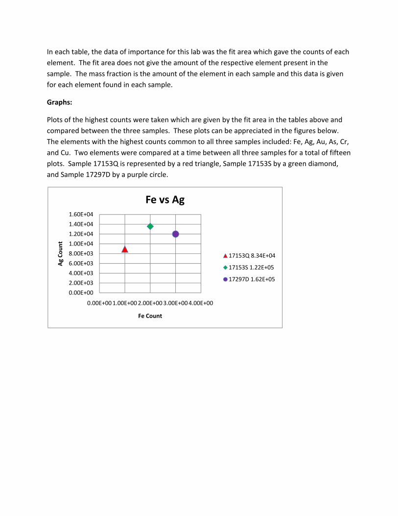
Graphs:

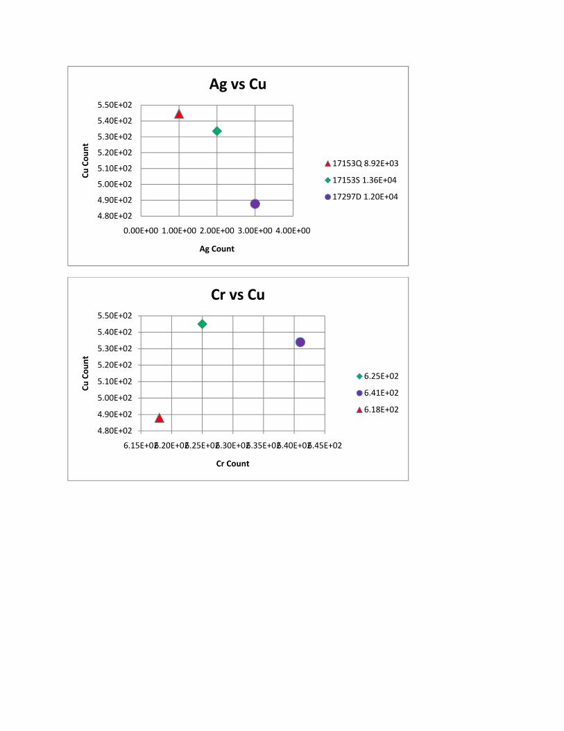
Plots of the highest counts were taken which are given by the fit area in the tables above and

compared between the three samples. These plots can be appreciated in the figures below.

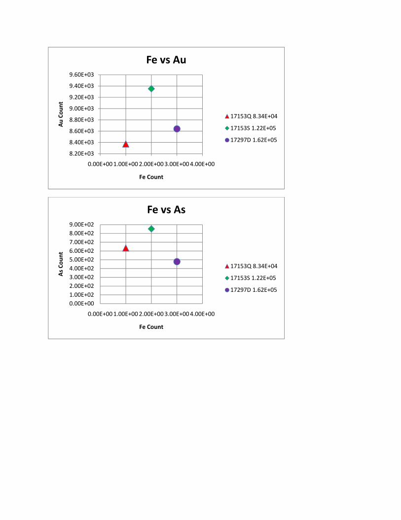
The elements with the highest counts common to all three samples included: Fe, Ag, Au, As, Cr,

and Cu. Two elements were compared at a time between all three samples for a total of fifteen

plots. Sample 17153Q is represented by a red triangle, Sample 17153S by a green diamond,

and Sample 17297D by a purple circle.

0.00E+00

2.00E+03

4.00E+03

6.00E+03

8.00E+03

1.00E+04

1.20E+04

1.40E+04

1.60E+04

0.00E+00 1.00E+00 2.00E+00 3.00E+00 4.00E+00

Ag

Co

un

t

Fe Count

Fe vs Ag

17153Q 8.34E+04

17153S 1.22E+05

17297D 1.62E+05

8.20E+03

8.40E+03

8.60E+03

8.80E+03

9.00E+03

9.20E+03

9.40E+03

9.60E+03

0.00E+00 1.00E+00 2.00E+00 3.00E+00 4.00E+00

Au

Co

un

t

Fe Count

Fe vs Au

17153Q 8.34E+04

17153S 1.22E+05

17297D 1.62E+05

0.00E+00

1.00E+02

2.00E+02

3.00E+02

4.00E+02

5.00E+02

6.00E+02

7.00E+02

8.00E+02

9.00E+02

0.00E+00 1.00E+00 2.00E+00 3.00E+00 4.00E+00

As

Co

un

t

Fe Count

Fe vs As

17153Q 8.34E+04

17153S 1.22E+05

17297D 1.62E+05

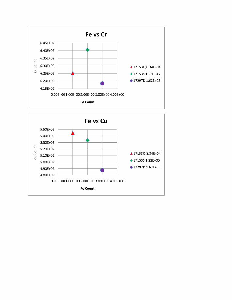
6.15E+02

6.20E+02

6.25E+02

6.30E+02

6.35E+02

6.40E+02

6.45E+02

0.00E+00 1.00E+00 2.00E+00 3.00E+00 4.00E+00

Cr

Co

un

t

Fe Count

Fe vs Cr

17153Q 8.34E+04

17153S 1.22E+05

17297D 1.62E+05

4.80E+02

4.90E+02

5.00E+02

5.10E+02

5.20E+02

5.30E+02

5.40E+02

5.50E+02

0.00E+00 1.00E+00 2.00E+00 3.00E+00 4.00E+00

Cu

Co

un

t

Fe Count

Fe vs Cu

17153Q 8.34E+04

17153S 1.22E+05

17297D 1.62E+05

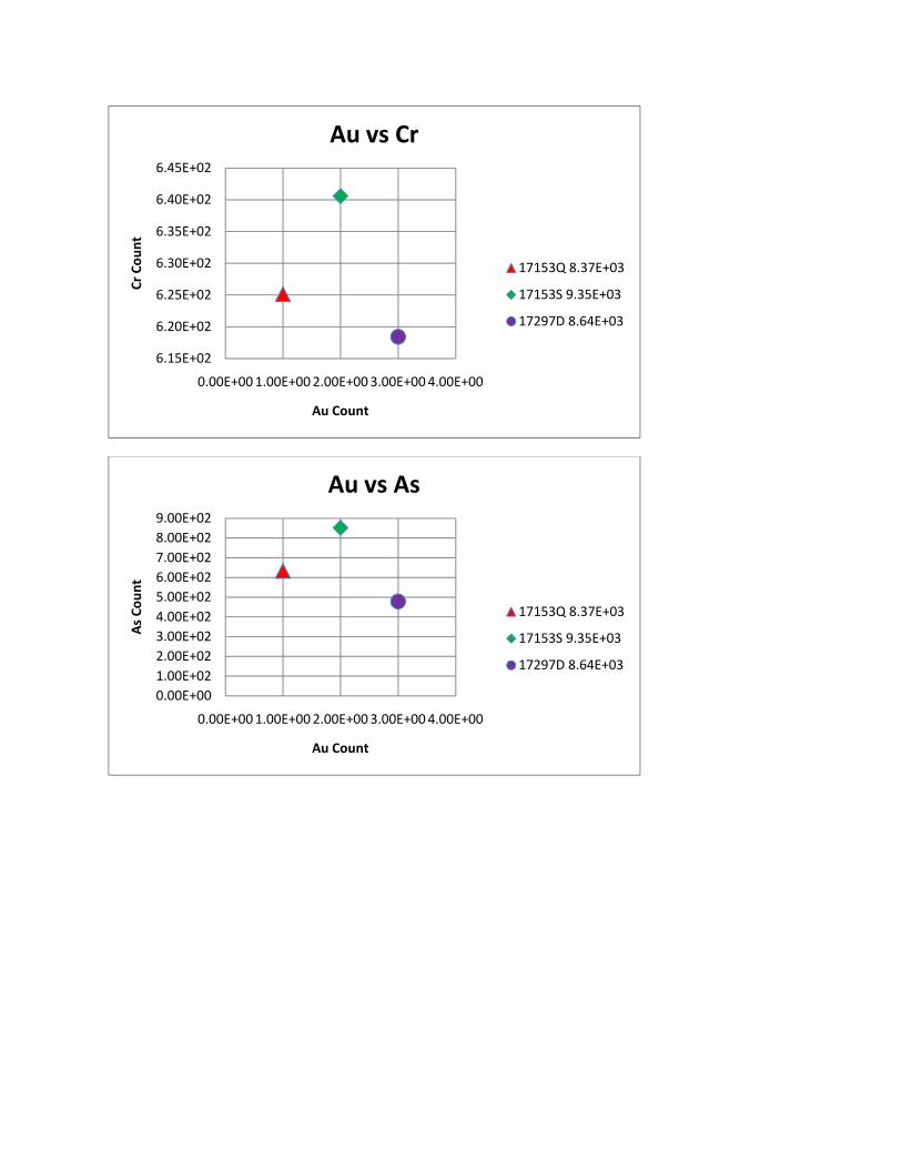
6.15E+02

6.20E+02

6.25E+02

6.30E+02

6.35E+02

6.40E+02

6.45E+02

0.00E+00 1.00E+00 2.00E+00 3.00E+00 4.00E+00

Cr

Co

un

t

Au Count

Au vs Cr

17153Q 8.37E+03

17153S 9.35E+03

17297D 8.64E+03

0.00E+00

1.00E+02

2.00E+02

3.00E+02

4.00E+02

5.00E+02

6.00E+02

7.00E+02

8.00E+02

9.00E+02

0.00E+00 1.00E+00 2.00E+00 3.00E+00 4.00E+00

As

Co

un

t

Au Count

Au vs As

17153Q 8.37E+03

17153S 9.35E+03

17297D 8.64E+03

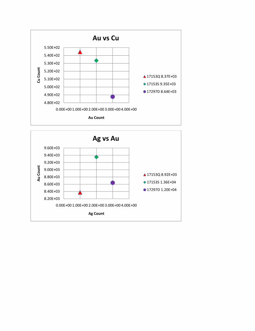
4.80E+02

4.90E+02

5.00E+02

5.10E+02

5.20E+02

5.30E+02

5.40E+02

5.50E+02

0.00E+00 1.00E+00 2.00E+00 3.00E+00 4.00E+00

Cu

Co

un

t

Au Count

Au vs Cu

17153Q 8.37E+03

17153S 9.35E+03

17297D 8.64E+03

8.20E+03

8.40E+03

8.60E+03

8.80E+03

9.00E+03

9.20E+03

9.40E+03

9.60E+03

0.00E+00 1.00E+00 2.00E+00 3.00E+00 4.00E+00

Au

Co

un

t

Ag Count

Ag vs Au

17153Q 8.92E+03

17153S 1.36E+04

17297D 1.20E+04

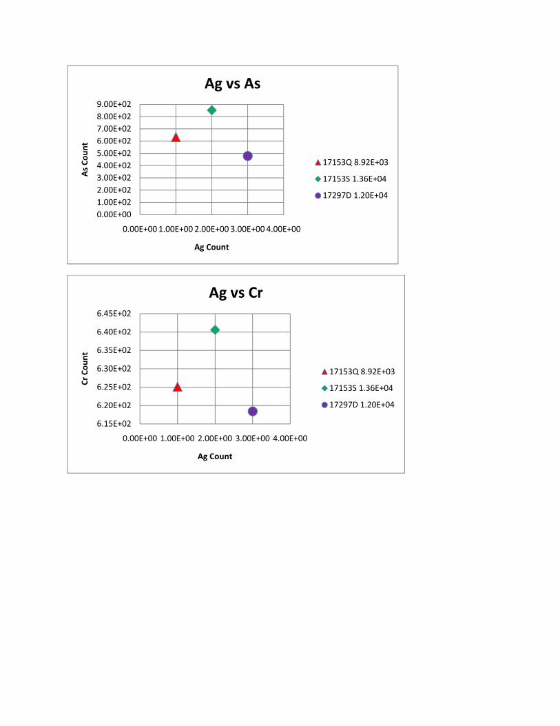
0.00E+00

1.00E+02

2.00E+02

3.00E+02

4.00E+02

5.00E+02

6.00E+02

7.00E+02

8.00E+02

9.00E+02

0.00E+00 1.00E+00 2.00E+00 3.00E+00 4.00E+00

As

Co

un

t

Ag Count

Ag vs As

17153Q 8.92E+03

17153S 1.36E+04

17297D 1.20E+04

6.15E+02

6.20E+02

6.25E+02

6.30E+02

6.35E+02

6.40E+02

6.45E+02

0.00E+00 1.00E+00 2.00E+00 3.00E+00 4.00E+00

Cr

Co

un

t

Ag Count

Ag vs Cr

17153Q 8.92E+03

17153S 1.36E+04

17297D 1.20E+04

4.80E+02

4.90E+02

5.00E+02

5.10E+02

5.20E+02

5.30E+02

5.40E+02

5.50E+02

0.00E+00 1.00E+00 2.00E+00 3.00E+00 4.00E+00

Cu

Co

un

t

Ag Count

Ag vs Cu

17153Q 8.92E+03

17153S 1.36E+04

17297D 1.20E+04

4.80E+02

4.90E+02

5.00E+02

5.10E+02

5.20E+02

5.30E+02

5.40E+02

5.50E+02

6.15E+026.20E+026.25E+026.30E+026.35E+026.40E+026.45E+02

Cu

Co

un

t

Cr Count

Cr vs Cu

6.25E+02

6.41E+02

6.18E+02

6.15E+02

6.20E+02

6.25E+02

6.30E+02

6.35E+02

6.40E+02

6.45E+02

0.00E+00 1.00E+00 2.00E+00 3.00E+00 4.00E+00

Cr

Co

un

t

As Count

As vs Cr

17153Q 6.33E+02

17153S 8.52E+02

17297D 4.78E+02

4.80E+02

4.90E+02

5.00E+02

5.10E+02

5.20E+02

5.30E+02

5.40E+02

5.50E+02

0.00E+00 1.00E+00 2.00E+00 3.00E+00 4.00E+00

Cu

Co

un

t

As Count

As vs Cu

17153Q 6.33E+02

17153S 8.52E+02

17297D 4.78E+02

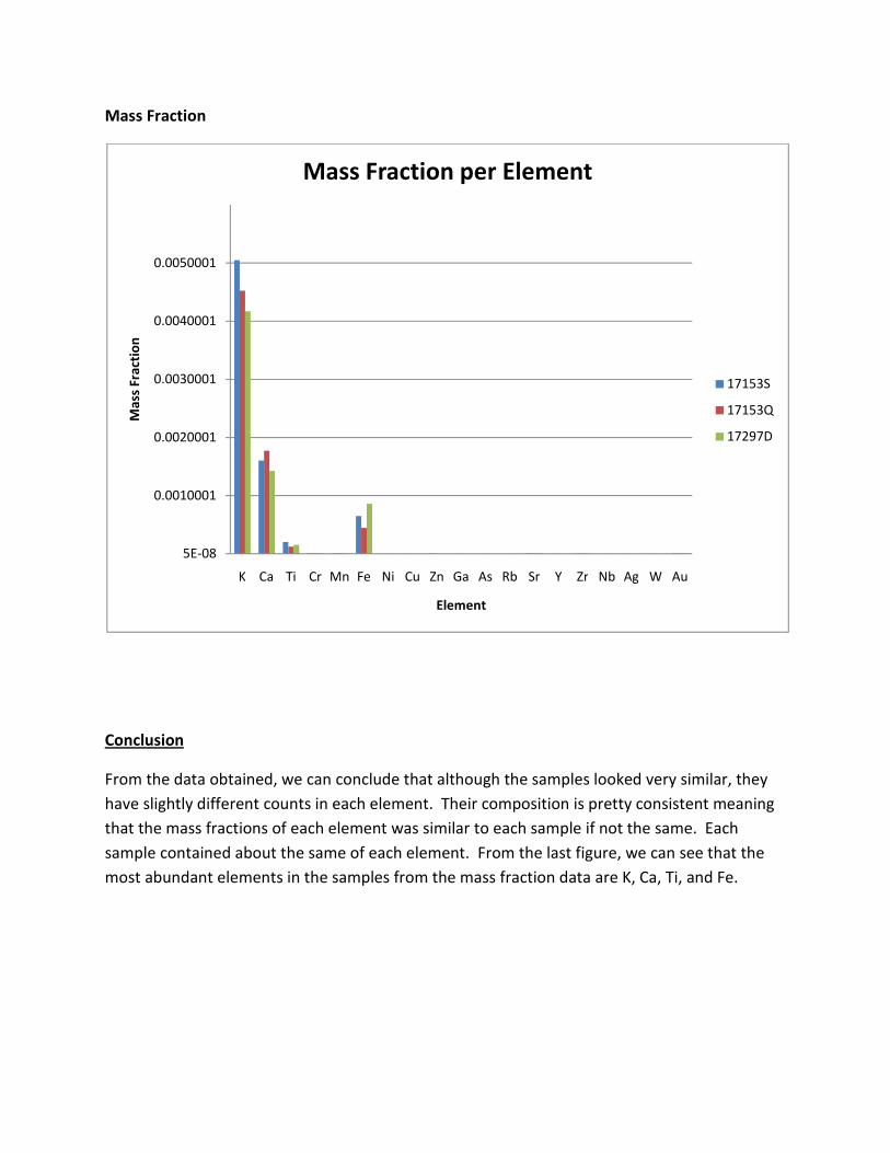
Mass Fraction

Conclusion

From the data obtained, we can conclude that although the samples looked very similar, they

have slightly different counts in each element. Their composition is pretty consistent meaning

that the mass fractions of each element was similar to each sample if not the same. Each

sample contained about the same of each element. From the last figure, we can see that the

most abundant elements in the samples from the mass fraction data are K, Ca, Ti, and Fe.

5E-08

0.0010001

0.0020001

0.0030001

0.0040001

0.0050001

K Ca Ti Cr Mn Fe Ni Cu Zn Ga As Rb Sr Y Zr Nb Ag W Au

Ma

ss F

ract

ion

Element

Mass Fraction per Element

17153S

17153Q

17297D

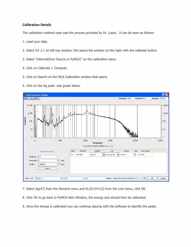
Calibration Details

The calibration method used was the process provided by Dr. Lopez. It can be seen as follows:

1. Load your data.

2. Select S# 2.1 on left top window; this opens the window on the right with the calibrate button.

3. Select “Internal(from Source or PyMCA)” on the calibration menu.

4. Click on Calibrate > Compute.

5. Click on Search on the MCA Calibration window that opens.

6. Click on the Ag peak –see graph below.

7. Select Ag(47) from the Element menu and KL3(0.54112) from the Line menu, click OK.

8. Click OK to go back to PyMCA Main Window, the energy axis should then be calibrated.

9. Once the energy is calibrated you can continue playing with the software to identify the peaks.

x-ray fluorescence lab report - dashboard -...

Documents