Working Paper 276December 2011

Quid Pro Quo: Builders, Politicians, and Election Finance in India

Abstract

In developing countries where elections are costly and accountability mechanisms weak, politicians often turn to illicit means of financing campaigns. This paper examines one such channel of illicit campaign finance: India’s real estate sector. Politicians and builders allegedly engage in a quid pro quo, whereby the former park their illicit assets with the latter, and the latter rely on the former for favorable dispensation. At election time, however, builders need to re-route funds to politicians as a form of indirect election finance. One observable implication is that the demand for cement, the indispensible raw material used in the sector, should contract during elections since builders need to inject funds into campaigns. Using a novel monthly-level data set, we demonstrate that cement consumption does exhibit a political business cycle consistent with our hypothesis. Additional tests provide confidence in the robustness and interpretation of our findings.

JEL Codes: P16; D72; E32Keywords: elections, election finance, corruption, political economy, India

www.cgdev.org

Devesh Kapur and Milan Vaishnav

Quid Pro Quo:Builders, Politicians, and Election Finance in India

Devesh KapurCenter for Global Developmentand University of Pennsylvania

Milan VaishnavCenter for Global Development

and Columbia University

Corresponding author: mv2191@columbia.edu. We would like to thank Owen McCarthy for excellent research assistance. We thank Matthew Levendusky, Philip Oldenburg, Neelanjan Sircar, Arvind Subramanian, Sandip Sukhtankar, and participants at the University of Pennsylvania and the Center for Global Development for comments. Milan Vaishnav would like to thank the Center for Global Development, the Center for the Advanced Study of India at the University of Pennsylvania, and the National Science Foundation (Doctoral Dissertation Improvement Grant SES #1022234) for financial assistance. All errors are our own.

CGD is grateful for contributions from the William and Flora Hewlett Foundation in support of this work.

Devesh Kapur and Milan Vaishnav. 2011. “Quid Pro Quo: Builders, Politicians, and Election Finance in India.” CGD Working Paper 276. Washington, D.C.: Center for Global Development. http://www.cgdev.org/content/publications/detail/1425795

Center for Global Development1800 Massachusetts Ave., NW

Washington, DC 20036

202.416.4000(f ) 202.416.4050

www.cgdev.org

The Center for Global Development is an independent, nonprofit policy research organization dedicated to reducing global poverty and inequality and to making globalization work for the poor. Use and dissemination of this Working Paper is encouraged; however, reproduced copies may not be used for commercial purposes. Further usage is permitted under the terms of the Creative Commons License.

The views expressed in CGD Working Papers are those of the authors and should not be attributed to the board of directors or funders of the Center for Global Development.

1

1. Introduction

In democracies across the developed and developing worlds, there is concern that the costs

of elections are growing unabated (Pinto-Duschinsky 2002). In the United States, the Federal

Election Commission calculates that candidates contesting the 2008 presidential election

spent nearly $1.8 billion, almost three times what was spent in the 2004 presidential election

cycle and almost four times the 1996 figures.1 On the other side of the globe, economists

estimate that candidates and parties in the 2009 Indian national elections spent roughly $3

billion on campaign expenditures. Election spending alone is said to have increased India’s

GDP growth by .5 percent for two quarters of 2009 (Timmons and Kumar 2009).

Yet one key difference between democracies in the developed and the developing worlds is

the alleged role that illicit election funds play in the latter. In developed democracies, there

are well-established systems of monitoring and accounting for election finance and for

prosecuting those involved in alleged improprieties. The strength of these systems likely

deters the transfer of illicit funds to a great extent.2 In developing countries, however,

scholars and observers have widely reported that illicit campaign finance expenditures often

dwarf legal flows. As one scholar has noted, this reality is often referred to as the “rule of

ten”—the idea that actual election expenditures are ten times the reported amounts

(Gingerich 2010). While there is a great deal of anecdotal evidence regarding the presence of

illicit (or “black”) money in elections, there has been little empirical analysis of these flows,

and for obvious reasons. By their very nature, flows of “black” money are opaque: they

involve under-the-table transfers that are largely unobservable and therefore difficult to

quantify. Yet black money can potentially undermine voters’ confidence in the democratic

process and can lead to severe governance failures.

In this paper, we examine one much-discussed channel of black money in Indian politics: the

construction and real estate sector. In recent years, there has been growing speculation of

cozy links between builders and politicians. The most common allegation proceeds along the

1 These figures are in nominal terms, and include primary and general election spending as well as the costs

of the nominating conventions. They do not include independent expenditures. See

http://www.fec.gov/press/press2009/20090608PresStat.shtml. 2 Of course, in countries such as the United States, there are real questions about the influence licit lobbying

expenditures and campaign finance donations from industry can have on legislator behavior. For recent examples

from the U.S. housing crisis, see Igan, Mishra and Tressel 2011; and Mian, Sufi and Trebbi 2010.

2

following lines. Politicians in India often accumulate substantial assets while in office, above

and beyond their official remuneration. In order to hide these assets from scrutiny and to

invest them productively, many politicians park these assets with builders involved in real

estate, a sector that has averaged annual growth rates of nearly ten percent over the last

decade. Builders require the aid of politicians because politicians have ensured that land

remains a highly regulated commodity over which the state has significant discretion.

Furthermore, the real estate sector perennially needs large volumes of liquidity, much larger

than banks are willing to finance. Thus, while politicians channel money to the sector and

provide discretionary access to land, builders in turn help to launder these funds safely in a

rapidly appreciating asset. More importantly for the purposes of this paper, at the time of

elections developers route part of these funds back to the politicians to help finance their

election campaigns. Although the aforementioned narrative is backed up by numerous

journalistic accounts as well as interviews with businessmen, politicians and government

officials conducted by the authors, this chain of events are nonetheless empirically unproven.

This paper seeks to address this lacuna by assessing empirically whether fluctuations in

construction activities are linked to electoral cycles in India. In so doing, it aims to shed light

on the acknowledged, though understudied, role of black money in Indian elections. While

we are not able to test each link in the causal chain empirically, we believe that the presence

of electoral cycles serves as suggestive evidence of the kinds of activities we describe here.

Specifically, we hypothesize that what money is to elections, cement is to construction—it is

the indispensible ingredient. Virtually all construction requires cement (for which there is no

material substitute), and the burgeoning real estate sector accounts for the majority of India’s

domestic cement demand. When construction activity increases, cement consumption rises

and vice versa. If therefore, the real estate sector is a key financier of elections, then just

prior to elections, builders will need to provide the liquidity to politicians to finance their

electoral campaigns. In turn, this will constrain the liquidity available to builders for their

own activities; as a result, construction activity should drop from the expected trend—and

so should cement consumption.

To assess the relationship between elections and activity in the real estate sector empirically,

we construct a novel panel dataset comprising information on the monthly consumption of

cement and the timing of elections in India’s 17 major states over the period 1995 to 2010.

Using an empirical model that controls for unobserved state and time-specific effects, we

investigate whether the presence of elections is associated with an observable drop in cement

consumption, which is consistent with a drying up of liquidity in the real estate sector

around election time.

To preview our findings, we find that there is a statistically significant contraction in cement

consumption (representing a 12 to 15 percent decline) during the month of state assembly

elections. This effect is slightly larger for scheduled elections, state (as opposed to national)

elections, dual elections (when elections to the state assembly and national parliament occur

concurrently), and for more urban states. To assess the robustness of this result, we use

randomization inference (Rader 2011) as a non-parametric method of testing the null

3

hypothesis that there is no relationship between elections and a decline in cement

consumption.

Having built confidence in our core finding, we address three plausible challenges to our

interpretation of the results: that the decline is indicative of a broader decline in economic

activity due to political uncertainty (or what some authors have called a “reverse business

cycle”); that builders should anticipate a liquidity crunch and smooth consumption over

time; and that decreases in cement consumption are due to a pre-electoral slowdown in

government investment. We demonstrate that these concerns do not invalidate our results.

Our findings have broad relevance for the study of money politics in the developing world,

where we are most likely to observe illicit election finance. There is a small, but growing

literature in this area (see Kupferschmidt 2009 for one review; and Gingerich 2010 for a

unique empirical example from Brazil). This paper adds to this literature in two ways. First, it

focuses on a specific sector—real estate—that is widely thought to be linked with “off-the-

books” politics across the developing world. Second, it contributes a novel measure for

capturing election cycles in this sector that is consistent with its role as a source of election

finance.

Our findings are also broadly related to the field of “forensic” economics, which has

developed innovative methods of estimating the private returns to political power. Work in

this area attempts to estimate the extent to which firms benefit from possessing political

connections (Fisman 2001; Johnson and Mitton 2003; Khwaja and Mian 2005; Faccio 2006;

Jayachandran 2006; and Goldman, Rocholl and So 2009). A second strand of the literature

attempts to identify the benefits politicians obtain on the basis of their political power

(Eggers and Hainmueller 2009; Querubin and Snyder 2011; Bhavnani 2011). In contrast to

this larger literature, we place an emphasis on the role of election finance incentives rather

than mere rent seeking (though one notable exception is Sukhtankar 2011).

Given the centrality of the election cycle to our argument, this paper is also linked to the

literature on political business cycles (Akhmedov and Zhuravskaya 2004; Khemani 2004; Shi

and Svensson 2006; Brender and Drazen 2005; Cole 2008). Yet, like Sukhtankar (2011), our

paper is unique in that our core hypothesis predicts a contraction in activity (within a specific

sector) around elections. This stands in contrast to much of the political business cycle

literature, which is premised around an expansion of economic activity around election time.

The remainder of the paper is organized as follows. In the next section we analyze the

drivers of election expenditures, including the shift toward private financing. We then briefly

review the workings of the alleged quid pro quo between politicians and builders and present

our hypotheses. In the fourth section, we outline the data and methods used to assess our

hypotheses empirically. Next, we present statistical evidence in support of our primary

hypotheses on election timing and cement consumption. To build confidence in the result,

we address some of the most plausible challenges to our interpretation of the findings.

Finally, we conclude by summarizing the implications of our findings for the literature,

4

emphasizing the need for a research agenda on the impact of election finance on democracy

and development outcomes.

2. The Indian context

Money is an essential ingredient of democratic politics; it is used to finance parties, mobilize

voters and conduct political campaigns. And there is a deeply held belief among students of

Indian politics that the costs of elections have skyrocketed in recent years. Taking a step

back, in the abstract we might postulate that democratic elections have become more costly,

with costs increasing in: a) the size of constituencies; b) the intensity of political competition;

c) the number of elections; and d) the weakness of non-electoral systems of accountability.

In our judgment, conditions a) through c) are clearly satisfied in India while d) presents a

mixed picture. But it is clear we are seeing an increasing flow of money for elections, as well

as a shift toward greater reliance on private mechanisms of campaign finance.

2.1 Factors influencing the cost of elections

First, as India’s population has grown, the size of political constituencies has ballooned.

While the median parliamentary constituency in 1952 (the date of India’s first post-

independence elections) had fewer than 300,000 voters, today’s parliamentary constituencies

contain between 1.5 and 2 million people. The growth in the size of the electorate over time

means that candidates have to spend more money to woo potential supporters.

Second, there has been a marked increase in the competitiveness of Indian elections. The

decline of the Congress system and the dawn of the coalition era in Delhi provided direct

incentives for leaders to form new parties (Ziegfeld 2010). According to Sridharan (2009),

the number of national parties declined from 8 to 6 between 1989-2004, while the number

of state parties increased from 20 to 36 and the number of registered parties doubled from

85 to 173.3 Competition has also added to electoral uncertainty, meaning that parties find it

increasingly difficult to calculate the elasticity of votes to expenditures.4

Third, the scope of elections has increased dramatically over the last two decades. The 73rd

and 74th Amendments to the Constitution (1992-1993) formally established a three-tier

system of democratic governance at the local levels, adding nearly 2.9 million new elected

positions to India’s democratic patchwork (and, hence, the increased need for election

finance). Political parties field candidates at all three levels, even at the village level where

formal partisan affiliations are prohibited, though regularly brandished.

3 In 1977, 2,439 candidates from 35 parties contested parliamentary elections across 543 parliamentary

constituencies. By 2009, the numbers had risen to 8,070 candidates and 207 parties. Authors’ calculations, based

on grouping Independents together as a single political party. The trends are similar for state assembly elections. 4 In the post-Congress era, an additional factor contributing to electoral uncertainty is incumbency

disadvantage (Uppal 2009).

5

Fourth, non-electoral mechanisms of accountability could help control the rising costs of

elections, yet their uneveness has limited their effectiveness. Political parties, for instance, are

poorly organized and weakly institutionalized; hence, they are not able (or willing) to regulate

election spending internally. Furthermore, parties are not able to cover the funds needed to

for contest elections from their own coffers. While all parties collect membership dues, they

are marginal to the cost of fighting elections. Without strong party organizations, candidates

have had to look elsewhere for creative ways to accumulate campaign-related resources.

State regulation of election finance could curb rising costs, but here too the results have been

disappointing. The thirst for election finance could be partially offset if elections were state

funded, which could curb the demand for private financing. But in India, state funding does

not exist. Furthermore, there is a yawning gap between de facto versus de jure election finance

regulations. Under law, parliamentary candidates cannot spend more than Rs. 1-2.5 million,

while assembly candidates can spend between Rs. 0.5-1.0 million (the exact amount varies by

state) per election, but these spending limits have unrealistically low ceilings and numerous

loopholes. On the contributions side, efforts to regulate corporate contributions have not

changed the under-the-table pattern of party funding. As Sridharan (2009) notes: “[T]he

potential costs and risks of transparency largely outweigh any tax benefits. In a still fairly

discretionarily regulated economy, transparent donors run the risk of being penalized by

parties in power at the state or center that are unhappy with who and in what amounts a

company donates funds.”

New disclosure requirements have also been, at best, a partial success. For instance,

candidates are required to disclose their campaign expenditures within 30 days of the

election, yet there is often no incentive for the candidates to comply because authorities have

very little motivation to follow up once the election is completed. And even when candidates

do disclose campaign expenditures, the disclosures are often farcical.5

It is, of course, difficult to create a proper accounting of the scale of illicit election finance. A

1999 independent election audit in 24 parliamentary constituencies found that the average

winner spent Rs. 8.3 million (when the limit ranged from 1.0-2.5 million) (Sridharan 2006).

Recent interdictions by the Election Commission of India (ECI) are also instructive. In

advance of the 2011 state assemly elections in Tamil Nadu, the ECI seized Rs. 600 million

(or $13.3 million) in illicit cash that was intended for election purposes (Economic Times, May

12, 2011).6 Of course, we do not know how much illicit money was actually spent, only what

5 The average candidate in the 2009 Lok Sabha elections reported spending around half the legal limit, a fact

that does not comport with the ground realities of Indian elections (ADR 2009). 6 In one instance, a ruling party aide was arrested while carrying illicit campaign cash along with a detailed

diary of distributions. In one municipal ward alone, the party distributed Rs. 2.4 million (Krishnan 2011). If we

assume these funds were distributed equally to all voters, this amounts to roughly Rs. 200 per voter (nearly seven

times the daily urban poverty rate of Rs. 33).

6

the ECI was able to recover through its investigative operations (which itself is likely a small

fraction).

Finally, other non-electoral mechanisms of accountability—namely civil society and the

media—have had mixed success tracking the money trail. Thanks to public interest litigation

filed by civil society organizations, the Supreme Court of India ruled in 2003 that all

candidates must disclose their personal financial assets/liabilities. These affidavits have shed

tremendous light on the influence of money in India’s elected bodies (Vaishnav 2011). Yet,

they contain no information on election expenditures. India has a long tradition of a free

media, and they too have often played a role in exposing improprieties in election finance.

Yet, unfortunately, some news organizations have become part of the problem themselves

(Economic and Political Weekly 2009). In 2010, the Press Council of India documented several,

high-profile instances of “cash for coverage,” whereby politicians and journalists exchanged

money for favorable coverage.

2.2 Mechanisms of private financing

The stylized facts of the Indian system described above point to incentives for private

financing of elections, which in turn, open the door to methods of “off-the-books” or illicit

financing. To quench the thirst for such financing, there are at least five mechanisms that

seem to be growing in intensity.

First, parties are actively recruiting candidates involved in serious criminal activity because

they possess both the financial resources and the connections necessary to contest elections

successfully. Vaishnav (2011) argues that one of the most important demand-side

explanations for the “criminalization” of politics in India is the fact that alleged criminal

candidates have significant financial assets at their disposal that allow them to self-finance.

Second, there is a growing number of businessmen directly contesting national elections.

Sinha (2010) estimates that businessmen constitute 22 percent of the Lok Sabha (lower

house of Parliament) and 16 percent of the Rajya Sabha (upper house of Parliament). These

figures represent significant increases over the last decade—and possibly understate the

increase, given the lack of transparency concerning members’ business interests.

Businessmen or not, the membership of elected bodies is increasingly being restricted to a

plutocratic minority. More than 50 percent of both chambers of parliament are crorepatis or

the Indian equivalent of millionaires ( one “crore” rupees is equivalent to Rs. 10 million or

about $225,000), while the average wealth of a state-level Member of the Legislative

Assembly (MLA) is 1.28 crores (Vaishnav 2011).

Third, wealthy individuals are not only contesting elections directly but they are also

bankrolling entire political movements. For instance, the Reddy bothers (a sibling trio of

mining magnates) from Karnataka have used their vast mining wealth to bankroll the BJP’s

rise to power in that state. As a reward, two of the three brothers received cabinet berths

while the third was awarded directorship of a powerful state corporation (Sanjana 2008).

7

Fourth, many parties are said to readily accept payment in exchange for party nominations

(“tickets,” in the Indian parlance). Indeed, Uttar Pradesh Chief Minister Mayawati readily

admitted that asking candidates to “make a donation to the party” was a key component of

her BSP party’s election strategy, with the proceeds derived from ticket buying used to

subsidize less well-off candidates (Pradhan 2006).

Finally, parties and their private sector allies launder funds through domestic and

international markets. Since the onset of economic liberalization in 1991 India has become

much more integrated with the global economy, making it easier to move money into and

out of the country. As a result, high net-worth individuals and participants in India’s

underground economy have begun stashing their assets abroad to take advantage of

generous foreign tax regimes. Assets sent abroad can also be repatriated for domestic use

under the guise of foreign investment and are widely reported to be a source of election

financing (Jaffrelot 2002).7 And funds can also be laundered domestically. It is one such

channel—real estate—that we turn to in the next section.

3. The real estate channel

To date, we are not aware of any scholarly empirical work that examines the connections

between the real estate sector and India’s political leaders. In this section, we describe why

the sector is an important conduit for illicit election finance.

3.1 The builder-politician nexus

We start with the premise that the more regulatory intensive the sector, the more its rent

extractive potential (Djankov et al. 2002). Indeed the major sources of political corruption

(and illicit election financing) in India come from the sectors that are most heavily regulated–

natural resources, spectrum allocation and defense—because they offer the most scope for

discretion by politicians.8 In the case of the real estate sector the need for regulatory

forbearance requires constant political favors because the acquisition and use of land is

intensely politically and bureaucratically regulated. As Pratap Bhanu Mehta (2010) writes,

“The discretionary power the state has with respect to land is the single biggest source of

corruption” in India.

7 A report by Global Financial Integrity, a Washington, DC-based think tank, estimates that between 1948

and 2008 India lost around $213 billion in illicit financial flows. The report surmises that these funds were the

product of corruption; bribery and kickbacks; criminal activity; and efforts by citizens to shelter their wealth from

domestic tax authorities (Kar 2011). 8 Indeed, some of India’s most infamous corruption scandals involved bribery and kickbacks whereby

politicians traded policy discretion for cash, some portion of which is alleged to have financed political activities.

These include the Bofors and Tehelka.com scandals (defense); the Madhu Koda case (mining); and the 2G

telecom scandal (spectrum).

8

Real estate has several attributes which makes it an obvious choice for black money. We

assume that it is easier for politicians to accumulate resources than to hide them. When

politicians want to hide the true value of their assets, they need a financial mechanism that

has the features of a bank without the traceability of a physical account. We stipulate the

mechanism should have at least three features:

a) Absorptive capacity: It should have the ability to absorb large amounts of money quickly and

directly

b) Liquid assets: It should be able to carry liquid assets (i.e. the money should be available

when needed)

c) Contract enforcement: It should offer some mechanisms for contract enforcement

Real estate possesses all these characteristics. As one of the principal industries in India—

recent estimates suggest real estate accounts for over seven percent of India’s Gross

Domestic Product (GDP)—it can absorb large volumes of cash. The Indian government

estimates that there will be a need to construct 26.5 million new houses to keep up with

current demand (Planning Commission 2008). Still, banks have been wary of lending to this

sector, for three reasons. First, banks are concerned about speculative bubbles in the

housing sector. Second, because many of the underlying land transactions are executed “in

the black” and might be of dubious legality, firms seeking funds might think twice about

seeking bank financing.9 Third, there are few barriers to entry for builders seeking to join the

marketplace, and banks are likely reluctant to finance builders without established track

records.

Finally, the sector’s regulatory intensity not only makes it a boon for raising funds but also

provides politicians with a mechanism to enforce its “contract” with builders. The rules that

governed land use a century ago are still in force today, as there is little incentive for

politicians to alter the status quo given the benefits that are accrued under the current system

(Pai 2011).10 The primary piece of legislation governing land acquisition (the Land

Acquisition Act) was written in 1894 by British colonial authorities. This and other laws,

such as the Urban Land Ceiling Act, created a regulatory structure that empowered

bureaucrats (and the politicians who oversee them) to control and manipulate the

distribution of urban land. The resulting bureaucratic maze has created myriad methods of

rent seeking (Srinivas 1991). The discretionary use of authority means that politicians can

also take steps to punish builders who do not support them during elections.

9 For instance, governments often sell land to private developers at sub-market rates, where the differential

between the government and market price is the size of the kickback. Firms cannot obtain official financing

based on the actual purchase price, because this would expose the corruption premium. 10

It is important here to distinguish between sectors of the economy that are under the purview of the

federal government and those that are state subjects. The liberalizing reforms that took place in India during the

early 1990s focused on the former category. The central government cannot mandate reform of sectors primarily

under the states’ control.

9

The affinity between builders and politics is not unique to India; in fact, the comparative

literature is littered with similar examples. One of the more memorable examples comes

from Chubb’s (1982) work on Palermo, Sicily. She describes the quid pro quos between

builders, the local administration and the mafia that shaped the city’s post-war urban

development. The sequence of events bears close resemblance to the situation in India.

Local Palermo politicians used their regulatory leverage to provide preferred access to

builders in exchange for political support and campaign contributions. Authors have

described similar scenarios in the Philippines (Sidel 1999); Thailand (Ockey 1998); and

machine-era America (Erie 1988, Chapter 2).11

3.1 How the quid pro quo works

In this section, we briefly review how the quid pro quo between politicians and builders

operates. There are three basic stages. In the first stage, politicians accumulate resources

while in office. Although the salaries for MLAs and Members of Parliament (MPs) are

modest, studies have shown that the asset holdings of many elected politicians are often

disproportionately large.12 Estimating the financial rewards to office is a difficult enterprise

due to the variety of ways politicians can hide their assets from public scrutiny, but in recent

years there have been numerous allegations of rent-seeking: chief ministers of at least six

states have been investigated for “disproportionate assets” (and a seventh has been arrested

for money laundering) (see also Bhavnani 2011).

Once politicians accumulate assets, they require a place to invest these assets where they can

avoid public scrutiny while earning a decent return. Because land is a valuable commodity

and India’s real estate industry is booming as the size of the middle class expands, many

politicians are thought to deposit a portion of their assets with real estate developers.

Politicians’ links with builders typically take three forms. First, relatives of politicians often

establish their own real estate development firms and reap the rewards from the value of

their familial connections. In other cases, politicians become covert backers of firms because

they represent powerful entities whose support must be won and retained.13 One illustrative

case comes from the prosperous Western state of Gujarat. A 2001 investigation by the news

magazine Outlook revealed that a quarter of ministers in the state cabinet had links with real

11 Although it is not a focus of this paper, many of the studies cited document a triangular connection

between the mafia or other organized crime groups, politicians and real estate/construction interests. See

Weinstein (2008) for one perspective on the illicit nexus between politicians, the bureaucracy and the mafia in

Mumbai’s real estate market. 12

A 2009 civil society analysis of re-contesting MPs reported their assets increased, on average, by 289

percent while in office (Thakur 2011). An econometric analysis found less outlandish gains, but concluded that

between 5-8 percent of MLAs and MPs have “suspect wealth” above what their official remuneration would

suggest (Bhavnani 2011). 13

While politicians have leverage over builders, the reverse is also true. One MP in Maharashtra, concerned

about a crackdown on state discretion over land, lamented: “Which builder will give you money during elections

if his work is not done?” (Khetan 2011).

10

estate developers. The politicians, the report argues, colluded with state-level bureaucrats

who granted favorable dispensation to the politician’s preferred builders (Bhushan 2001).

On occasion politicians will have a direct financial stake in real estate development.

Typically, however, his or her interest begins as a secret, and only becomes public knowledge

when scandals erupt. For example, the recent history of Maharashtra contains numerous

examples of powerful state politicians with direct or indirect financial interests in real estate,

whose interests are not a matter of public record until civil society groups or the media

expose the connection (Khetan 2011).14

In the third and final stage of the quid pro quo, builders transfer back to politicians assets

that can be used to offset election expenses. In the case of family-owned firms, politicians

can embezzle or transfer funds from family firms as a way of channeling money for elections

(as in Sukhtankar 2011). When there is no direct familial connection, the mechanism can be

a simple under-the-table transfer or an in-kind contribution. Although builders have to

transfer funds back to politicians around elections, the transaction brings long-term benefits

in terms of future favors, permits, and goodwill.15

Recent revelations from India’s massive 2G telecommunications spectrum scandal provide

some limited insight into these hypothesized stages of the quid pro quo. In early 2011, the

government charged A. Raja, the Union Minister of Telecommunications, with underpricing

the sale of the 2G telecommunications spectrum and manipulating the spectrum allocation

process in favor of selected companies.16 According to the government, Raja, an MP from

Tamil Nadu and a confidant of that state’s Chief Minister, helped a telecom company (which

served as a front for the country’s third largest real estate developer) win access to 2G

licenses. The government alleges that the developer transferred around $40 million in

kickbacks, through a serious of shadowy transactions emanating from real estate entities, to a

television network controlled by the family of Tamil Nadu’s Chief Minister (Shenoy 2011).

3.2 Hypotheses on cement consumption

Analyzing activity in India’s real estate sector, both over time and at the sub-national level,

presents difficulties for measurement. Unlike in many developed economies, there are no

reliable measures of building activity—at last at sufficiently meaningful levels of

disaggregation. To circumvent this shortcoming, we use data on the amount of cement that

is consumed in the major states of India on a monthly basis over a 15-year period. Cement

consumption represents a suitable proxy for real estate building activity for two reasons.

14 One investigation into the builder-politician nexus in Maharashtra suggests that in Mumbai, “almost every

MLA and MP, both past and present, cutting across party lines, owns at least one real estate project, either

directly or through family members or a proxy, at any given point in time” (Khetan 2011). 15

A former Congress MLA is quoted as remarking: “For builders, raising funds for candidates during

elections is not a favour, but a transaction which can be encashed at a later date” (India Realty News 2009). 16

India’s comptroller estimates the improprieties could have caused losses to the government worth around

$39 billion.

11

First, cement is the indispensable ingredient in virtually all real estate construction; it has no

obvious substitute as a binding agent for building materials. As such, it is a reasonable

barometer for construction activity. Second, industry research estimates that real estate

accounts for between 65 and 75 percent of India’s domestic cement demand (with

infrastructure accounting for the remainder) (India Brand Equity Foundation n.d.). Thus, we

are confident that changes in the extent of building activity are highly correlated with

fluctuations in cement consumption.

Our core hypothesis is that cement consumption should contract during the month of the

election (denoted in the analysis as Election). Because real estate developers must transfer

back to politicians resources invested with them as elections near, one would expect activity

in the sector to slow down during the four-week campaign period prior to Election Day.

This is because existing liquidity in the sector should dry up as resources otherwise slated for

construction must be channeled out of the sector and into the hands of politicians and

parties (Hypothesis #1).

Next, we hypothesize that the contraction in cement demand should be larger during

scheduled elections (Scheduled Election) compared to unscheduled elections. When elections

occur on time (once every five years), builders and politicians have an ex ante schedule to

guide their transactions. When unscheduled elections are held— say, if a government loses a

vote of no confidence and/or the government falls—it might be more difficult for builders

to adjust their activities accordingly. We expect that, in the case of scheduled elections, there

is sufficient time for politicians and builders to coordinate (Hypothesis #2). Furthermore,

since elections in a parliamentary system can be considered endogenous, it could be the case

that unscheduled elections are related to economic factors that are correlated with changes in

the real estate sector. We can address this by separating out the effects of scheduled versus

unscheduled elections.

In India’s federal system, the state—as opposed to the national government—is the primary

regulator of the land and building activity sectors. Hence, rents emanating from real estate

are more relevant for state level politicians, while rents from spectrum or defense deals

accrue to politicians at the national level. However, we expect that we should still observe a

significant effect for national elections as firms also stand to benefit from connections to

politicians in parliament. Therefore, we expect that the contraction in cement consumption

will be significant in national elections (Lok Sabha Election), though of a smaller magnitude

than in state-level elections (Hypothesis #3).

Yet, elections in some states coincide with national elections; for instance, the last three state

assembly elections in Andhra Pradesh (in 1999, 2004 and 2009) have coincided with national

parliamentary elections. In those instances, which we refer to as dual elections (Dual Election),

the need for election finance will be greater; therefore, we expect the magnitude of the

contraction to be larger than if only a state or national election is being held (Hypothesis #4).

12

Finally, more urbanized states are comparatively richer; are more likely to possess well-

developed real estate markets; and have higher demand for construction—and therefore,

cement—than their rural counterparts. As a result, linkages between politicians and builders

are likely to be more intense in urban states (Urban). Thus, we expect that the negative

impact of elections on cement consumption should be stronger in more urban states

(Hypothesis #5).

4. Data and methods

To test our hypotheses, we construct a novel dataset of monthly data on cement

consumption, disaggregated by state. The source of the data is the Cement Manufacturers’

Association of India (CMA), an industry trade group whose members include the country’s

largest public and private sector cement manufacturers. One of CMA’s primary roles is to

serve as a comprehensive clearinghouse for information on the capacity, production,

dispatch and export of cement, using data collected from its member companies. CMA’s

data are proprietary but were provided to the authors by a member company. Monthly data

on cement consumption (measured in metric tons) is available from April 1995 to March

2010, for a total of 180 calendar months per state. We utilize data on cement consumption,

rather than production, because our hypotheses on electoral cycles revolve around

contractions in liquidity in the real estate sector, which is heavily dependent on the use of

cement. In other words, we do not make any claims about linkages between electoral politics

and the supply of cement (production).17

India is a federal parliamentary democracy comprised of 28 states and 7 union territories.

For our analysis on cement consumption, we focus on the 17 major states of the union,

which account for over 92 percent of the country’s population, for several reasons. First, we

do not include data from the three new states created in 2000 (Chhattisgarh, Jharkhand and

Uttarakhand) because we cannot disaggregate data on cement consumption before their

creation. Second, we ignore several small microstates, which we treat as special cases because

their economies are not comparable to their larger peers. Third, we do not consider the

union territories for a similar reason and because they do not have elected assemblies.18

However, we do include the union territory of Delhi because it does have its own elected

assembly and is a major economic center. According to data from 2009-2010, cement

consumption in the 17 major states accounts for 90 percent of the all-India total. Thus, we

are comfortable that we are working with data that has considerable explanatory power.

17 Having said that, we are aware of the numerous direct political connections many of India’s largest

cement firms possess. Several of India’s major cement firms are owned by the Birla family, one of the country’s

most storied business dynasties, while one of the other major sectoral players is the state-owned Cement

Corporation of India, Ltd. 18

Union territories are directly administered by the central government, with the exception of Delh and

Puducherry.

13

To our dataset on cement consumption, we add information on state elections. Data on the

frequency and timing of elections comes from the ECI. Between April 1995 and March

2010, there were a total of 52 state elections across India’s 17 major states as well as five

national parliamentary elections (1996, 1998, 1999 and 2004, 2009). Roughly one-quarter of

all state elections in our dataset coincide with parliamentary elections. State assembly

elections take place every five years, although a state assembly can be dissolved before the

conclusion of its full term and early elections can be called. Of the 52 state elections in our

dataset, only 9 were unscheduled (roughly 17 percent). Of the 5 national elections, 2 were

unscheduled.

To test for electoral cycles in cement consumption, we adapt the model used by Akhmedov

and Zhuravskaya (2004) in their study of opportunistic political business cycles in Russia.

These authors construct a dataset of elections and monthly budgetary expenditures in

Russia’s states in order to identify the influence of political opportunism on government

spending. Although their subject is different, their model suits our empirical puzzle quite

nicely. Specifically, we estimate the following equation using regional monthly panel data:

log yit jm jit 1yit1j{6;6}

t f is it, (1)

where i identifies states, t represents the month of the year, and y stands for the level of

cement consumption (in log terms) in a given state-month (Log Cement Consumption).

m jit is

an indicator variable that equals one, when t is j months away from the state election. Our

model includes time fixed effects,

t , where there is an indicator for each month-year. This

fixed effects parameter controls for unobserved national-level trends as well as any general

macroeconomic shocks. As in Akhmedov and Zhuravskaya (2004), we also need to control

for state-specific fixed effects as well as any state-specific seasonal or time shocks. Hence, we

include the fixed effects term,

f is , for each of the twelve calendar months of the year (s) in

each state, i.

Our primary variable of interest is

m jit when j = 0, which signifies the month of the state

election (Election). In the base specification, we also include dummies for each of the six

months preceding and following a state election (Election-1, Election-2, etc). A negative

coefficient on

j when j = 0 would provide support for our hypothesis that the occurrence

of a state election is associated with a drop in cement consumption.

Finally, we include a lag of our dependent variable,

yit1, in the model because we want to

explicitly model the temporal dependence in our data. We believe there are strong theoretical

reasons for expecting that cement consumption in a given month is likely to be influenced

14

by earlier levels of consumption. Furthermore, we are concerned about the presence of serial

correlation in the data, so including a lag makes sense from a modeling perspective.19

Using the Akaike information criterion (AIC), we tested for optimal lag selection. In half of

the diagnostic tests (run separately for each state), the results suggested we should include

three lags of the dependent variable, while half of the tests indicated we should include four

lags. The regressions below include three lags, but the results do not change if we include

four lags (results available on request). In addition, we tested for unit roots using the test

developed by Im, Pesaran and Shin (2003). Based on the mean of the individual Dickey-

Fuller t-statistics of each unit in the panel, the Im-Pesaran-Shin test assumes that all series

are non-stationary under the null hypothesis. Based on the test statistics, we can reject the

null hypothesis of non-stationarity. We estimate all models using Ordinary Least Squares

(OLS), using the correction for panel-corrected standard errors (PCSE) suggested by Beck

and Katz (1995) to deal with non-spherical errors (heteroskedasticity and contemporaneous

correlation).

5. Results

5.1 Baseline analysis

Summary statistics for the data used in this cement analysis can be found in Table 1.

Table 1: Summary statistics

Variable Obs Mean Std. Dev. Min Max

Election 3060 0.02 0.13 0 1

Scheduled election 3060 0.01 0.12 0 1

Lok Sabha election 3060 0.03 0.16 0 1

Scheduled Lok Sabha election 3060 0.02 0.13 0 1

Dual election 3060 0.00 0.06 0 1

Log cement consumption 3060 5.97 0.87 2.59 7.76

Urban 3060 0.53 0.50 0 1

Log cement production 2698 5.44 1.73 0 8.07

First, we proceed with our baseline series of multivariate regressions in which we estimate

the effect of state elections on (log) cement consumption. As seen in Column 1 of Table 2

we begin by estimating our model without any fixed effects parameters and only including

indicator variables for the election month and the six months before and after. The

19 We tested for serial correlation using Wooldridge’s test for serial correlation in linear panel data using the

Stata command, -xtserial-. The results indicate that we cannot reject the null hypothesis of no serial correlation in

the data.

15

regression results indicate that state elections are associated with a 12 percent decline in

cement consumption. There is a slight increase in cement consumption immediately after the

election, but otherwise the coefficient of the election lags and leads are insignificant.

This simple specification does not control for time trends, so in Column 2 we add time fixed

effects—or indicator variables for every month-year combination. In Column 3, we include

only state-month fixed effects to account for state-specific seasonality in construction

activity. Finally, in Column 4, we include both time and seasonal fixed effects parameters (as

in Equation 1 above). Across all models, our results show that the occurrence of a state

election is associated with a statistically significant decline in cement consumption (p<.01).

Table 2: Baseline estimates of the effect of state elections on cement consumption

-1 -2 -3 -4

DV: Log cement consumption

Log cement consumption

Log cement consumption

Log cement consumption

election-6 0.02 0.02 0.04 0.06

[0.78] [0.73] [1.54] [2.69]***

election-5 -0.01 0.00 -0.02 0.00

[0.42] [0.04] [0.88] [0.03]

election-4 0.00 -0.01 -0.02 -0.02

[0.12] [0.38] [0.84] [0.69]

election-3 -0.03 -0.03 -0.03 -0.03

[1.08] [1.19] [1.21] [1.55]

election-2 0.04 0.03 0.02 0.01

[1.27] [1.24] [0.83] [0.55]

election-1 0.04 0.02 -0.01 0.01

[1.38] [0.85] [0.31] [0.21]

election -0.12 -0.12 -0.12 -0.13

[4.12]*** [4.71]*** [4.87]*** [5.44]***

election+1 0.09 0.05 0.03 0.03

[2.95]*** [1.97]** [1.33] [1.29]

election+2 0.02 0.04 0.03 0.03

[0.82] [1.50] [1.19] [1.17]

election+3 0.03 0.04 0.07 0.04

[0.89] [1.40] [3.06]*** [1.56]

election+4 -0.01 -0.02 0.03 0.01

[0.28] [0.57] [1.16] [0.63]

election+5 -0.04 -0.01 0.02 0.04

[1.46] [0.25] [0.98] [1.82]*

election+6 -0.03 -0.04 -0.01 0.01

[1.05] [1.65]* [0.51] [0.20]

Fixed effects? - Time State-Month Time +

State-Month

Observations 2856 2856 2856 2856

Number of states 17 17 17 17

R-squared 0.95 0.96 0.97 0.97 Note: Z statistics in brackets. * significant at 10%; ** significant at 5%; *** significant at 1%. All models

include three lags of the dependent variable. Models are estimated using OLS with panel-corrected standard

errors. Dependent variable is natural log of cement consumption

16

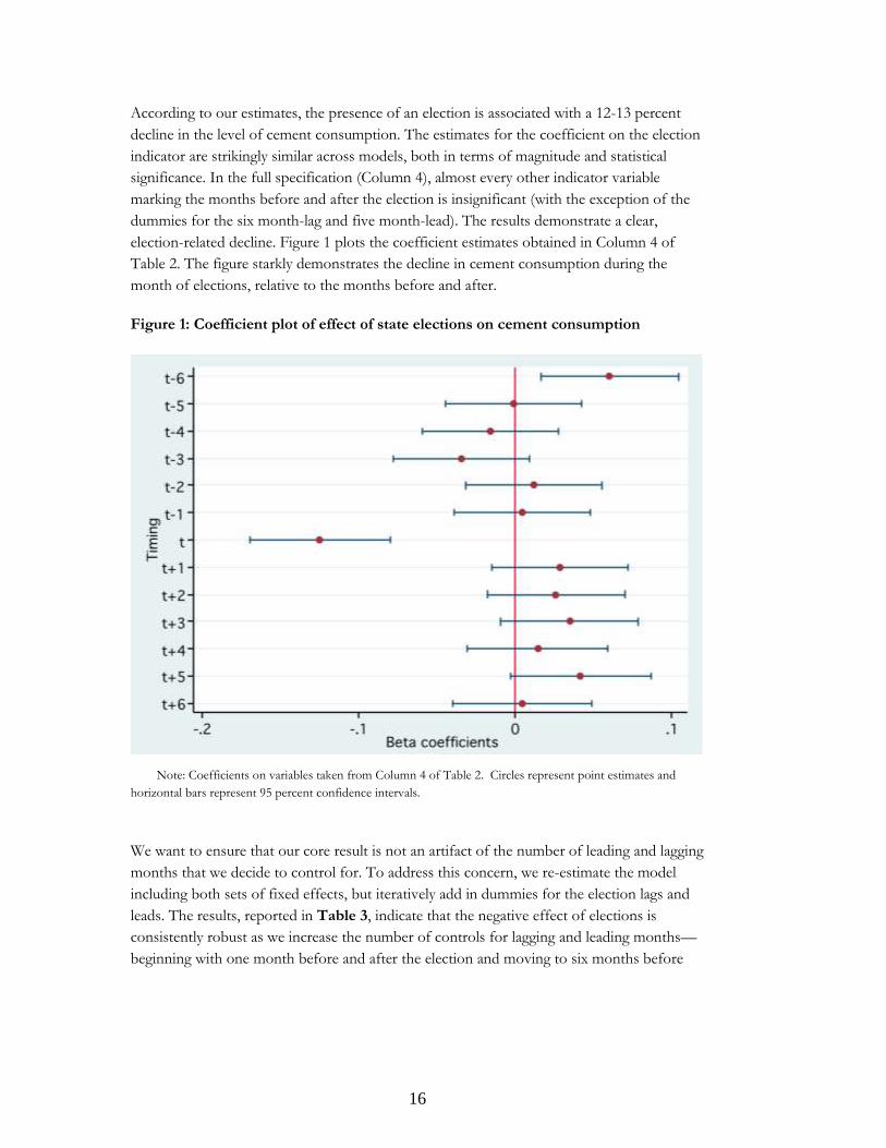
According to our estimates, the presence of an election is associated with a 12-13 percent

decline in the level of cement consumption. The estimates for the coefficient on the election

indicator are strikingly similar across models, both in terms of magnitude and statistical

significance. In the full specification (Column 4), almost every other indicator variable

marking the months before and after the election is insignificant (with the exception of the

dummies for the six month-lag and five month-lead). The results demonstrate a clear,

election-related decline. Figure 1 plots the coefficient estimates obtained in Column 4 of

Table 2. The figure starkly demonstrates the decline in cement consumption during the

month of elections, relative to the months before and after.

Figure 1: Coefficient plot of effect of state elections on cement consumption

Note: Coefficients on variables taken from Column 4 of Table 2. Circles represent point estimates and

horizontal bars represent 95 percent confidence intervals.

We want to ensure that our core result is not an artifact of the number of leading and lagging

months that we decide to control for. To address this concern, we re-estimate the model

including both sets of fixed effects, but iteratively add in dummies for the election lags and

leads. The results, reported in Table 3, indicate that the negative effect of elections is

consistently robust as we increase the number of controls for lagging and leading months—

beginning with one month before and after the election and moving to six months before

17

Table 3: Baseline estimates of the effect of state elections on cement consumptions, varying lags and leads

-1 -2 -3 -4 -5 -6

DV: Log cement consumption

Log cement consumption

Log cement consumption

Log cement consumption

Log cement consumption

Log cement consumption

election-6 0.06

[2.69]***

election-5 0.00 0.00

[0.04] [0.03]

election-4 -0.02 -0.01 -0.02

[0.66] [0.62] [0.69]

election-3 -0.03 -0.03 -0.03 -0.03

[1.39] [1.43] [1.55] [1.55]

election-2 0.01 0.01 0.01 0.01 0.01

[0.46] [0.48] [0.53] [0.50] [0.55]

election-1 0.00 0.00 0.00 0.00 0.00 0.01

[0.10] [0.09] [0.13] [0.15] [0.20] [0.21]

election -0.12 -0.12 -0.12 -0.12 -0.12 -0.13

[5.46]*** [5.46]*** [5.45]*** [5.48]*** [5.47]*** [5.44]***

election+1 0.03 0.03 0.03 0.03 0.03 0.03

[1.42] [1.43] [1.42] [1.49] [1.34] [1.29]

election+2 0.03 0.03 0.03 0.03 0.03

[1.39] [1.32] [1.26] [1.22] [1.17]

election+3 0.04 0.03 0.04 0.04

[1.56] [1.49] [1.54] [1.56]

election+4 0.01 0.01 0.01

[0.46] [0.53] [0.63]

election+5 0.04 0.04

[1.72]* [1.82]*

election+6 0.01

[0.20]

Fixed effects? Time + State-

Month Time + State-

Month Time + State-

Month Time + State-

Month Time + State-

Month Time + State-

Month

Observations 2992 2975 2958 2924 2890 2856 Number of states 17 17 17 17 17 17

R-squared 0.98 0.98 0.97 0.98 0.97 0.97

18

and after. Indeed, in results not reported here, the results are consistent even if we include

dummies for a larger set of months before and after the election.20

5.2 Scheduled elections

We hypothesized that the contraction in cement consumption will be larger for scheduled

elections because they provide politicians and builders with some degree of certainty that

allows them to coordinate activities. It is also important to distinguish between scheduled

and unscheduled elections because election timing is not strictly exogenous. Hence, there is a

concern that governments might call early elections for some reason that might also be

correlated with changes in the economy that could impact the demand for cement. Our

results for scheduled elections can be found in Column 1 of Table 4. Even when using this

restricted measure, the occurrence of state elections continues to have a negative effect on

cement consumption. In line with our expectations, the coefficient on the scheduled state

election variable is slightly larger than when we considered all state elections (scheduled or

not). Cement consumption declines by 15 percent during the month of scheduled elections

(p<.01).

5.3 Dual elections

We hypothesized that there should be a stronger negative effect of elections on cement

consumption in those states that are experiencing simultaneous state and national elections.

As Column 2 of Table 4 attests, the negative effect of dual elections on cement

consumption is nearly three times as strong as that of state elections (and more than twice as

strong as unscheduled state elections). Dual elections are associated with a 38 percent drop

in the level of cement consumption (p<.01). This result suggests the imperative for election

finance is significantly larger when candidates for state and national elections need to raise

funds for their respective campaigns simultaneously.

5.4 Urban-rural states

We hypothesized that the effect of elections of cement consumption should be larger in

urban states. To classify states, we take advantage of population figures provided in the 1991

and 2001 census. We use the urban/rural population figures from the 1991 census to create

a dichotomous indicator for urban/rural states for the years 1995-2000. Using the 2001

census, we do the same for the years 2001-2010. We code states as urban if their urban

population is above the median for all states, and rural otherwise.21 Columns 3 and 4 of

Table 4 confirm our hypothesis. While elections are associated with a decline in cement

20 The estimates are remarkably consistent when we control for up to 11 months of lags and leads. When

we control for the 12 months lagging and leading the election, the size of the effect declines as does the

significance (p<.05). 21

The classification for the two periods is identical, with the exception of Haryana—which moves in to the

“urban” category after 2001.

19

consumption in both urban and rural states, the effect is much stronger for urban states (15

percent decline versus 11 percent) as well as more significant.

Table 4: Disaggregating estimates of the effect of elections on cement consumption,

by election type

-1 -2 -3 -4

DV: Log cement consumption

Log cement consumption

Log cement consumption

Log cement consumption

Sample: Urban states Rural states

election-6 0.06 0.05 0.09 0.06

[2.76]*** [2.06]** [3.12]*** [1.53]

election-5 0.00 -0.01 0.00 0.01

[0.04] [0.45] [0.00] [0.39]

election-4 -0.02 -0.01 0.03 -0.06

[0.67] [0.46] [0.85] [1.69]*

election-3 -0.03 -0.02 -0.04 -0.03

[1.55] [1.00] [1.44] [0.86]

election-2 0.01 0.02 0.00 0.04

[0.54] [0.96] [0.04] [1.03]

election-1 0.00 -0.01 0.00 0.00

[0.19] [0.26] [0.12] [0.09]

election -0.02 -0.15 -0.11

[1.05] [4.95]*** [3.04]***

election+1 0.03 0.02 0.06 -0.01

[1.27] [1.06] [1.91]* [0.17]

election+2 0.03 0.01 0.05 0.00

[1.20] [0.56] [1.77]* [0.10]

election+3 0.04 0.06 0.07 0.02

[1.56] [2.61]*** [2.21]** [0.50]

election+4 0.02 0.03 0.01 0.03

[0.63] [1.29] [0.34] [0.74]

election+5 0.04 0.03 0.06 0.01

[1.87]* [1.17] [1.78]* [0.38]

election+6 0.00 0.00 0.02 -0.01

[0.20] [0.17] [0.66] [0.20]

scheduled_election -0.15

[5.58]***

dual_election -0.38

[5.86]***

lok_sabha_election 0.00

[0.10]

Fixed effects? Time +

State-Month Year +

State-Month Time +

State-Month Time +

State-Month

Observations 2856 2856 1512 1344

Number of states 17 17 9 8

R-squared 0.97 0.97 0.92 0.98

20

Table 5: Estimates of the effect of national elections on cement consumption

-1 -2 -3 -4 -5

DV: Log cement consumption

Log cement consumption

Log cement consumption

Log cement consumption

Log cement consumption

Lok Sabha election-6 0.03 0.04 -0.03 -0.01 -0.01

[0.67] [0.91] [1.12] [0.34] [0.30]

Lok Sabha election-5 0.02 0.03 0.00 0.02 0.02

[0.39] [0.65] [0.11] [0.60] [0.62]

Lok Sabha election-4 0.08 0.09 0.04 0.05 0.05

[1.93]* [2.06]** [1.45] [2.01]** [2.07]**

Lok Sabha election-3 0.05 0.05 0.02 0.02 0.02

[1.26] [1.14] [0.59] [0.88] [0.82]

Lok Sabha election-2 -0.02 -0.02 0.00 0.01 0.01

[0.46] [0.40] [0.06] [0.48] [0.54]

Lok Sabha election-1 0.04 0.03 -0.05 -0.04 -0.04

[0.96] [0.77] [2.04]** [1.50] [1.55]

Lok Sabha election -0.10 -0.10 -0.06 -0.05

[2.58]*** [2.37]** [2.26]** [2.01]**

Lok Sabha election+1 0.03 0.03 -0.04 -0.04 -0.04

[0.81] [0.63] [1.51] [1.48] [1.52]

Lok Sabha election+2 0.00 0.00 0.01 0.01 0.00

[0.03] [0.06] [0.51] [0.26] [0.16]

Lok Sabha election+3 0.03 0.02 0.07 0.06 0.06

[0.64] [0.48] [2.76]*** [2.56]** [2.58]***

Lok Sabha election+4 -0.04 -0.05 0.02 0.04 0.03

[1.14] [1.07] [0.93] [1.40] [1.34]

Lok Sabha election+5 -0.05 -0.05 -0.02 -0.01 0.00

[1.35] [1.26] [0.83] [0.23] [0.15]

Lok Sabha election+6 0.02 0.02 -0.03 0.00 0.00

[0.56] [0.52] [1.02] [0.11] [0.14]

Scheduled Lok Sabha election -0.08

[2.56]**

Fixed effects? - Year State-Month Year +

State-Month Year +

State-Month

Observations 2856 2856 2856 2856 2856

Number of states 17 17 17 17 17

R-squared 0.95 0.95 0.97 0.97 0.97

Note: Z statistics in brackets. * significant at 10%; ** significant at 5%; *** significant at 1%. All models include three lags of

the dependent variable. Models are estimated using OLS with panel-corrected standard errors. Dependent variable is natural log of

cement consumption.

21

5.5 National elections

Thus far, we have focused on the effect of state assembly elections on cement consumption.

In Table 5, we explore the impact of national elections on cement consumption. As

hypothesized previously, we expect that the negative effect of elections on cement

consumption will be significant, though smaller, for national elections given that both land

and real estate/construction are regulated at the state-level. To estimate the effect of national

elections on cement consumption, we use a slightly different empirical model. Namely, we

can no longer include a full set of month-year fixed effects to account for the time trend

because the indicator for Lok Sabha (national) elections does not vary across states (e.g.

national elections are a common “shock” simultaneously experienced by all states in a given

month-year). Thus, in the regressions we can only include fixed effects for years as well as

for each state-month combination (e.g. seasonal time effects). Column 1 of Table 5 reports

the results of the baseline model (with no fixed effects). According to this basic

specification, national elections are associated with a 10 percent decline in cement

consumption (p<.01). In Columns 2 and 3, we add year fixed effects and seasonal effects,

respectively. The result holds although the coefficient is smaller (-.06) once seasonal effects

are included. In Column 4, we include both sets of fixed effects and the results here indicate

that national elections are associated with a 5 percent decline in the level of cement

consumption (p<.05). As for scheduled national elections, we find that the negative impact is

slightly more pronounced, as shown in Column 5. This effect is analogous to the differential

impact of scheduled versus unscheduled state elections. Column 5 reports an 8 percent

decline in cement consumption for scheduled national parliamentary elections (p<.05).

5.6 Randomization inference

To build confidence in our result, we make use of randomization inference, which is a non-

parametric method of hypothesis testing that does not rely on asymptotic properties or

distributional assumptions regarding the error terms in a model. This is particularly relevant

to our case, as we are working with panel data where we are likely to have “clustering” or

correlation among error terms within a particular group (in our case, states). In the models

described above, we addressed this issue using panel-corrected standard errors (PCSEs). Yet,

we might be concerned about the robustness of these estimates as we have a relatively small

number of clusters (states).

The basic procedure of conducting a randomization test is relatively straightforward and

proceeds in four steps, as outlined by Rader (2011).22 First, we estimate our baseline model

using OLS. We record the t-statistic on our election variable. Next, rather than taking the t-

statistic on our variable of interest at face value, we shuffle the variable. By randomizing the

election month variable, we are theoretically breaking any systematic connection between it

and the dependent variable. In the next step, we use this shuffled variable (in place of the

22 One recent empirical application of randomization inference in political science is Erikson, Pinto and

Rader (2010).

22

observed variable) to re-estimate the model. We repeat the randomization and estimation

1,000 times. By doing this, we create a reference distribution of t-statistics that would arise if

the null hypothesis were true. Finally, we can compare the observed t-statistic with the

reference distribution to determine what percentage of the time we observe a significant,

spurious effect. If the observed t-statistic is larger than 95 percent of the simulated t-

statistics, we can be confident in rejecting the null hypothesis of no relationship between

elections and cement consumption.

We use the model in Column 4 of Table 2 as our baseline regression, but without using the

correction for panel-corrected standard errors. The t-statistic on the election variable is 5.21.

Figure 2 graphically demonstrates the reference distribution of 1,000 t-statistics we obtained

from the randomization test. The vertical reference line indicates the t-statistic on our

baseline model. As the figure demonstrates, more than 95 percent of the time we obtain

results that are of lesser statistical significance than in our baseline model.

Figure 2: Randomization test results

Note: Baseline model used to obtain original estimated t-statistic adapted from Column 4 of Table 2. The

difference in t-statistics reported there and in this figure is due to the fact that we do not use panel-corrected

standard errors when conducting the randomization test. Otherwise, the underlying models are identical.

23

6. Robustness

Thus far, we have demonstrated empirically that there is a robust, negative relationship

between cement consumption and elections. We believe this is suggestive of real estate’s role

as a key financier of elections. In this section we address three of the most obvious

challenges to our interpretation of the results.

6.1 Economic uncertainty

What if the decline in cement consumption is not symptomatic of the real estate sector’s role

as a conduit for election finance, but instead the outcome of a broad decline in economic

activity arising out of political uncertainty that often precedes elections? For instance, Canes-

Wrone and Park (2010) argue that, in OECD countries, the political uncertainty associated

with elections induces private sector actors to postpone investments with high costs of

reversal. Hence, elections are associated with a decline in economic activity—a “reverse

business cycle”—as opposed to an economic expansion predicted by the literature on

opportunistic cycles.

Our results do not support such a view in the context of India for three reasons. First, we

find that there is a decline in cement consumption in both scheduled as well as unscheduled

elections. One would expect, given the uncertainty attached to unscheduled elections (often

sparked by political instability) that the pace of economic activity might naturally slow down

as business grapples with a potential change in government. Nonetheless, we find the decline

in cement consumption is larger in scheduled elections, when there is arguably less uncertainty.

Second, as an additional robustness test, we run our empirical model using monthly data on

cement production, rather than cement consumption, as our dependent variable. Recall, we

are primarily interested in election shocks to cement consumption (demand). If builders face

a liquidity shock during elections, we should not necessarily detect any systematic effect on

cement production (supply).23 But if production significantly declines during elections itself,

one could contend that our results on consumption are merely symptomatic of a larger

economic or sectoral cycle (rather than a demand-side shock).

As demonstrated by Table 6, we find no clear evidence of an electoral cycle in cement

production. Across all models, state elections are not associated with a significant change in

cement production. The results are also displayed in graphical form in Figure 3. The

coefficients on our election indicator variable are positive when we include the fixed effects

parameters, though they do not reach statistical significance. As for the months preceding

the elections, there does appear to be a contraction in production three months prior to the

elections. However, this decline is only half as large as the consumption decline we observe

23 Of course, it is plausible that cement producers will anticipate a decline in consumption and cut

production prior to elections. If this were the case, we should expect that some of the dummies for months

preceding elections to be positive and significant.

24

around elections. Furthermore, there are signs of a slight growth in cement production two

months prior to the elections. Overall, we can conclude that there is no indication of an

overall economic shock during the month of elections.

Table 6: Estimates of the effects of state elections on cement production

-1 -2 -3 -4

DV: Log cement production

Log cement production

Log cement production

Log cement production

Election-6 -0.01 -0.03 -0.02 -0.02

[0.24] [0.92] [0.67] [0.73]

Election-5 -0.02 -0.01 -0.02 -0.04

[0.50] [0.45] [0.69] [1.31]

Election-4 0.00 0.00 -0.04 -0.04

[0.02] [0.03] [1.63] [1.35]

Election-3 -0.03 -0.02 -0.06 -0.06

[0.88] [0.79] [2.17]** [2.18]**

Election-2 0.11 0.08 0.07 0.05

[3.31]*** [2.74]*** [2.40]** [1.71]*

Election-1 0.01 -0.04 -0.03 -0.04

[0.20] [1.18] [1.11] [1.56]

Election -0.03 0.03 0.01 0.03

[0.88] [0.91] [0.23] [1.04]

Election+1 0.01 -0.02 0.00 0.01

[0.27] [0.54] [0.16] [0.47]

Election+2 -0.05 -0.04 -0.01 -0.03

[1.37] [1.43] [0.44] [1.12]

Election+3 -0.02 -0.02 0.01 -0.02

[0.53] [0.63] [0.47] [0.60]

Election+4 0.01 0.01 0.03 0.02

[0.30] [0.21] [1.19] [0.83]

Election+5 -0.03 -0.01 0.01 0.01

[0.83] [0.41] [0.52] [0.37]

Election+6 0.01 -0.01 0.00 0.00

[0.14] [0.25] [0.08] [0.07]

Fixed effects? - Time State-Month Time +

State-Month

Observations 2514 2514 2514 2514

Number of states 15 15 15 15

R-squared 0.99 0.99 0.99 0.99

Note: Z statistics in brackets. * significant at 10%; ** significant at 5%; *** significant at 1%. All models

include two lags of the dependent variable. Models are estimated using OLS with panel-corrected standard

errors. Dependent variable is natural log of cement consumption. Delhi and Haryana are dropped due to

missing data.

25

Figure 3: Coefficient plot of effect of state elections on cement production

Note: Coefficients on variables taken from Column 4 of Table 6. Circles represent point estimates and

horizontal bars represent 95 percent confidence intervals.

Third, we can utilize data on the level of industrial production to examine whether the

decline in cement consumption is robust to controlling for the pace of general economic

activity. To control for the state of the economy, we utilize the index of industrial

production (IIP), an aggregate statistic that represents the status of production in the

industrial sector for a given period of time compared to a previous reference period. Since

the IIP is a national-level measure, we cannot use this data to analyze state elections.

However, we can use it as a control in our regressions looking at national elections. The

inclusion of the IIP variable does not substantively alter our estimates of the negative effect

of national elections on cement consumption (as seen in Table 7).

Finally, it is worth noting that the argument that general economic activity contracts on

account of election-induced uncertainty stands in contrast to much of the literature on

political business cycles in developing countries. Indeed, the literature on opportunistic

business cycles suggests that policymakers in developing democracies induce short-term

economic expansions (and increase deficits) before elections (Brender and Drazen 2005; Shi

and Svensson 2006). Studies of India have reached similar conclusions (Cole 2008; Khemani

2004).

26

Table 7: Estimates of the effect of national elections on cement consumption,

controlling for IIP

-1 -2 -3 -4

DV: Log cement consumption

Log cement consumption

Log cement consumption

Log cement consumption

Lok Sabha election-6 0.03 0.04 -0.02 0.00

[0.73] [0.90] [0.83] [0.03]

Lok Sabha election-5 0.02 0.03 0.00 0.02

[0.45] [0.66] [0.06] [0.67]

Lok Sabha election-4 0.08 0.09 0.04 0.05

[1.98]** [2.07]** [1.52] [2.16]**

Lok Sabha election-3 0.05 0.05 0.02 0.03

[1.31] [1.12] [0.75] [1.04]

Lok Sabha election-2 -0.02 -0.02 0.01 0.01

[0.41] [0.41] [0.28] [0.57]

Lok Sabha election-1 0.04 0.03 -0.04 -0.04

[1.01] [0.75] [1.71]* [1.44]

Lok Sabha election -0.10 -0.10 -0.05 -0.05

[2.53]** [2.36]** [2.18]** [2.00]**

Lok Sabha election+1 0.03 0.03 -0.03 -0.03

[0.86] [0.62] [1.43] [1.22]

Lok Sabha election+2 0.00 0.00 0.01 0.00

[0.07] [0.06] [0.24] [0.17]

Lok Sabha election+3 0.03 0.02 0.06 0.06

[0.67] [0.49] [2.56]** [2.39]**

Lok Sabha election+4 -0.04 -0.05 0.02 0.03

[1.11] [1.06] [0.90] [1.09]

Lok Sabha election+5 -0.05 -0.05 -0.02 -0.01

[1.32] [1.25] [0.79] [0.55]

Lok Sabha election+6 0.03 0.02 -0.01 -0.01

[0.64] [0.52] [0.45] [0.19]

IIP 0.00 0.00 0.00 0.00

[0.79] [0.11] [10.55]*** [2.46]**

Fixed effects? - Year State-Month Year +

State-Month

Observations 2856 2856 2856 2856

Number of states 17 17 17 17

R-squared 0.95 0.95 0.97 0.97

Note: Z statistics in brackets. * significant at 10%; ** significant at 5%; *** significant at 1%. All models

include three lags of the dependent variable. Models are estimated using OLS with panel-corrected standard

errors. Dependent variable is natural log of cement consumption.

6.2 Consumption smoothing

Another possible objection to our findings relates to the behavior of builders. For instance,

if builders anticipate the future need to redirect funds to election campaigns, why wouldn’t

27

they take action to smooth their consumption? After all, private firms (and economic agents,

in general) are said to prefer a stable consumption path over time. Thus, if firms know that

their consumption will likely decline in the future, they should anticipate this by gradually

redirecting funds over time rather than waiting for the month of elections.

While an impulse to “smooth” consumption makes sense in theory, we argue that it does not

happen in practice for two reasons. First, politicians provide funds to builders precisely

because they need a place to hide their assets from scrutiny. If builders redirected funds to

politicians in installments, it would undermine politicians’ incentives to move the assets off

their balance sheets this way. Instead, politicians want funds during election season because

they can route these funds into campaigns immediately, without keeping them on their own

books.

Second, because builders operate in a “black money” environment, there are constraints on

their liquidity that hamper their ability to smooth consumption. There are three reasons for

this. First, as was mentioned earlier, banks are generally cautious about lending to the real

estate sector. For instance, Reserve Bank of India (RBI) regulations mandate that banks’

exposure to real estate lending be no more than 15 percent of a bank’s total deposits (RBI

2009).24 Indeed, it is instructive to note that while the U.S. economy was severely hampered

by a mortgage-lending crisis in 2007-8, India avoided a similar fate thanks to conservative

lending practices and increased regulation in sectors such as real estate. Second, banks are

unlikely to provide builders with financing to address liquidity constraints in advance of

elections when the underlying motivations are expressly political. Third, election-season

borrowing is likely to be costly for builders because the cost of borrowing will increase if the

general demand for credit is higher as elections approach.

Of course, it is also possible that builders accept that idea that providing election finance—

and thus facing a short-term liquidity shortage—is part of the cost of doing business in a

highly regulated economy. Builders may be willing to put up with a temporary slowdown in

building activity if they are reaping benefits from the state in other ways.

6.3 Model code of conduct

A third possible objection to our findings concerns the rules of the ECI. From the time

elections are announced to the date results are made public, the ECI enforces a “model code

of conduct,” which is a set of guidelines that govern the conduct of the incumbent

government as well as parties and candidates taking part in elections. One of the motivations

of the model code is to create a level playing field so that the government does not exploit

the benefits of incumbency for electoral purposes.

24 Indeed, Patnaik, Shah and Suri (2011) find that penetration of commercial finance in the real estate sector

is very low in India.

28

One might argue that the decrease in cement consumption during the month of elections is

a direct result of the enforcement of the model code because it constrains the ability of the

government to carry out its regular business, which could include a variety of infrastructure

projects. Yet the model code only restricts the government from announcing new schemes

and projects in advance of the elections (Singh 2011). It has no bearing on the government’s

undertaking of existing projects. Given the time lag inherent in tenders, contracts, siting, etc.

we do not think this is biasing our results.

Furthermore, governments are likely to be strategic (especially when elections take place as

scheduled) in announcing new schemes prior to the formal enforcement of the model code

prior to elections. Doing so allows them to minimize the possibility of a slowdown in

projects come election time. For instance, as elections approach the incumbent government

has an incentive to get as much money out to contractors working on ongoing government

contracts (the quid pro quo is that contractors often lend their vehicles for campaigns). This

is consistent with Khemani (2004), who finds election-related increases in public investment

spending and spending on road expansion using subnational data from India.25

7. Conclusion

The presence of black money is a well-known feature of elections in many developing

democracies. Yet due to its opacity, much of what we know about illicit election finance is

based on anecdotal evidence or journalistic investigations. This paper represents a

contribution to a new literature, which seeks to use new or innovative sources of data to

demonstrate empirically —and quantify—the flows of black money in elections.

The role of the real estate sector in providing off-the-books campaign contributions to

politicians has been a hallmark in many developing economies due to the nature of state

regulations governing land use. This paper uses variation in the demand for cement to

demonstrate the presence of an electoral cycle in building activity, using data from India.

This effect is consistent with the belief that the sector serves as a key conduit of black

money in elections. Using a variety of models, we demonstrate that our key empirical finding

is robust. Furthermore, we address what we see are the leading objections to our

interpretation of the underlying mechanism.

We believe that this work has several implications for the field of political economy. First,

scholars need to pay greater attention to the role black money is playing across the

developing world. If there are large sums of money moving through the political system

independent of official expenditures, our estimates of election finance will be downward-

25 One interpretation of our finding is that building activity slows down during elections because laborers in

the real estate sector are being used as temporary labor for campaigns. This is an interesting hypothesis for which

we would need additional data; but we believe this can be seen in our framework as an “in-kind” contribution

from builders.

29

biased if we do not take them into account. To date, much of the comparative literature

focuses on licit flows (see Scarrow 2007 for a review), but such flows likely constitute but a

fraction of total election spending in many developing countries.

Second, the growing expense of elections has serious implications for public policy in

developing countries. Raising money from “supporters” has the potential effect of post-

election paybacks in terms of distorting public policies. Indeed, the builder-politician nexus

has implications for decisions on land acquisition and conversion; land and housing prices

and land inequality; and the overall public management of urbanization.26

Third, election finance (its sources and methods) has ramifications for how democracy

functions. In principle, greater political competition, decentralization (i.e. greater number of

elected sub-national bodies), and more frequent elections can enhance citizen accountability

of elected representatives. But each of these benefits also comes with a financial cost with

respect to increasing electoral expenditure. While one could argue that costly elections can

serve as a screening device to weed out non-serious candidates, if privileged access to

resources becomes a pre-condition for winning election, this could have obvious effects on

the nature of political selection. Finally, there is the troubling prospect of the long-term

cognitive implications if election financing results in negative selection effects and a broader

corruption of the body politic. If the resulting cynicism among voters leads them to lose

faith in the democratic process, there will be little left to hold up the edifice itself.

26 The title of a recent article in the New York Times on Gurgaon, one of the fastest growing and richest

cities in India, says it all: “In India Dynamism meets Dysfunction” (Yardley 2011).

30

Bibliography

Akhmedov, A. and E. Zhuravskaya. 2004. “Opportunistic Political Cycles: Test in a Young

Democracy Setting.” Quarterly Journal of Economics 119(4): 1301-1338.

Association for Democratic Reforms. 2009. Analysis of the MPs of the 15th Lok Sabha

(2009): High-Level Summary. http://groups.google.co.in/group/national-ew-

news/browse_thread/thread/ea94c77fc5e04845?hl=en# (July 1, 2011).

Beck, N. and J. Katz. 1995. “What to Do (and Not to Do) With Time-Series Cross-Section

Data.” American Political Science Review 89(3): 634–47.

Bhavnani, R. 2011. “A Primer on Corruption Amongst India’s Politicians.” Working Paper.

Princeton University.

Bhushan, R. 2001. “Builders and Friends.” Outlook India. February 19.

http://www.outlookindia.com/article.aspx?210880 (July 2, 2011).

Brender, A. and A. Drazen. 2005. “Political Business Cycles in New Versus Established

Democracies.” Journal of Monetary Economics 52(7): 1271-1295.

Canes-Wrone, B. and J. Park. 2010. “Electoral Business Cycles in OECD Countries.”

Working Paper. Princeton University.

Chubb, J. 1982. Patronage, Power and Poverty in Southern Italy: A Tale of Two Cities. New York:

Cambridge University Press.

Cole, S. 2008. “Fixing Market Failures or Fixing Elections? Elections, Banks, and

Agricultural Lending in India.” American Economic Journals: Applied Economics 1(1): 219-

250.

Djankov, S et al. 2002. “The Regulation of Entry.” Quarterly Journal of Economics 117(1): 1-37.

Economic and Political Weekly. 2009. “Fourth Estate on Sale.” December 12.

Economic Times. 2011. “Election Commission Seizes Maximum Cash, 80% of the Rs. 74.27

Crore, in Tamil Nadu.” May 12.

Eggers, A. and J. Hainmueller. 2009. “MPs for Sale? Returns to Office in Postwar British

Politics.” American Political Science Review 103(4): 513-533.

Erie, S. 1990. Rainbow's End: Irish-Americans and the Dilemmas of Urban Machine Politics, 1840-

1985. Berkeley, CA: University of California Press.

Erikson, R., P. Pinto and K. Rader. 2010. “Randomization Tests and Multi-Level Data in

U.S. State Politics.” State Politics and Policy Quarterly 10(2): 180-198.

Faccio, M. 2006. “Politically Connected Firms.” American Economic Review 96(1):

369–86.

Fisman, R. 2001. “Estimating the Value of Political Connections.” American Economic Review

91(4): 1095–1102.

Gingerich, D. 2010. “Dividing the Dirty Dollar: The Allocation and Impact of Illicit

Campaign Funds in a Gubernatorial Contest in Brazil.” Working Paper. University of

Virginia.

Goldman, E., J. Rocholl and J. So. 2009. “Do Politically Connected Boards Affect Firm

Value?” The Review of Financial Studies 22(6): 2331-2360.

Igan, D., P. Mishra, and T. Tressel. 2011. “A Fistful of Dollars: Lobbying and the Financial

Crisis.” Working Paper 17076. National Bureau of Economic Research.

31

Im, K., M. Pesaran, and Y. Shin. 2003. “Testing for Unit Roots in Heterogeneous Panels.”

Journal of Econometrics 115: 53-74.

India Brand Equity Foundation. n.d. Cement. Report prepared for Confederation of Indian

Industry.

India Realty News. 2009. “Donation to Political Parties Worries Builders.” March 14.

http://www.indianrealtynews.com/real-estate-india/mumbai/donation-to-political-

parties-worries-builders.html (June 30, 2011).

Jaffrelot, C. 2002. “Indian Democracy: The Rule of Law on Trial.” India Review 1(1): 77-120.

Jayachandran, S. 2006. “The Jeffords Effect.” Journal of Law and Economics

49(2): 397–425.

Johnson, S., and T. Mitton. 2003. “Cronyism and Capital Controls: Evidence from

Malaysia.” Journal of Financial Economics 67(2): 351-382.

Kar, D. 2010. The Drivers and Dynamics of Illicit Financial Flows from India: 1948-2008.

Washington, DC: Global Financial Integrity.

Khemani, S. 2004. “Political Cycles in a Developing Economy: Effect of Elections in the

Indian States.” Journal of Development Economics 73(1): 125-154.

Khetan, A. 2011. “Land Grab. And How to Make Millions.” Tehelka 8(21). May 28.

Khwaja, A., and A. Mian. 2005. “Do Lenders Favor Politically Connected

Firms? Rent Provision in an Emerging Financial Market.” Quarterly Journal of Economics

120(4): 1371–1411.

Krishnan, Nandini. 2011. “Why Didn’t They Vote? Consipracy Theories Abound Post TN

Elections.” Sify News. http://www.sify.com/news/why-didn-t-they-vote-conspiracy-

theories-abound-post-tn-elections-imagegallery-national-letph8bgffg.html (June 26,

2011).

Kupferschmidt, D. 2009. “Illicit Political Finance and State Capture.” Background Paper.

International IDEA.

Mehta, P. 2010. “It’s the Land, Stupid.” Indian Express. August 19.

Mian, A., A. Sufi, and F. Trebbi. 2010. “The Political Economy of the Subprime Mortgage

Credit Expansion.” Working Paper 16107. National Bureau of Economic Research.

Ockey, J. 1998. “Crime, Society and Politics in Thailand” in Carl A. Trocki, ed.

Gangsters, Democracy and the State in Southeast Asia. Ithaca, NY: Cornell University Press.

Pai, S. 2011. “Our Land of Discontents.” Indian Express. May 20.

Patnaik, I., A. Shah and A. Suri. 2011. “Managing Boom and Bust in Real Estate: What

Lessons Can India Offer?” Working Paper. National Institute of Public Finance and

Policy.

Pinto-Duschinsky, M. 2002. “Financing Politics: A Global View.” Journal of Democracy 13(4):

69-86.

Planning Commission, Government of India. 2008. Eleventh Five-Year Plan (2007–2012).

Volume 3. New Delhi: Oxford University Press.

Pradhan, S. 2006. “I Take Money for Tickets: Mayawati.” Rediff. June 25.

http://www.rediff.com/cms/print.jsp?docpath=//news/2006/jun/05maya.htm (June

21, 2011).

32

2011. ”Wealth Accumulation by U.S. Congressmen, 1845-

1875: Were the Civil War Years Exceptional(ly Good)?” Working Paper. Harvard

University.

Rader, K. 2011. “Randomization Tests and Inference with Grouped Data.” Working Paper.

Columbia University.

Reserve Bank of India, Government of India. 2009. Master Circular on Exposure Norms and

Statutory/Other Restrictions – UCBs. July 1.

Sanjana. 2008. “The Reddy Flag Over Bangalore.” Tehelka 5(23). June 14.

Scarrow, S. 2007. “Political Finance in Comparative Perspective.” Annual Review of Political

Science 10: 193-210.

Shenoy, T.V.R. 2011. “DMK: More Bad News on the Way.” Rediff. March 16.

http://www.rediff.com/news/column/column-dmk-2g-corruption-tamil-

nadu/20110316.htm (July 1, 2011).

Shi, M., and J. Svensson. 2006. “Political Budget Cycles: Do They Differ Across Countries

and Why?” Journal of Public Economics 90(8-9): 1367-1389.

Sidel, J. 1999. Capital, Coercion and Crime: Bossism in the Philippines. Stanford, CA: Stanford

University Press.

Singh, U. 2011. “Between Moral Force and Supplementary Legality: A Model Code of

Conduct in Indian Elections.” Working Paper. Delhi University.

Sinha, A. 2010. “Business and Politics,” in Niraja Gopal Jayal and Pratap Bhanu Mehta, eds.

The Oxford Companion to Politics in India. New Delhi: Oxford University Press.

Sridharan, E. 2006. “Electoral Finance Reform: The Relevance of International Experience,”

in Vikram Chand, ed. Reinventing Public Service Delivery in India. New Delhi: Sage.

Sridharan, E. 2009. “Party System Fragmentation, Intra-Part Democracy, and Opaque

Political Finance.” CASI India in Transition Series.

http://casi.ssc.upenn.edu/iit/esridharan (June 1, 2011).

Srinivas, L. 1991. “Land and Politics in India: Working of Urban Land Ceiling Act, 1976.”

Economic and Political Weekly. October 26: 2482-2484.

Sukhtankar, S. 2011. “Sweetening the Deal? Political Connections and Sugar Mills in India.”

Working Paper. Dartmouth College.

Thakur, A. 2011. “MLAs’ Fortunes Grow More Than All Other Investments.” Times of India.

May 19.

Timmons, H. and H. Kumar. 2009. “India’s National Election Spread Millions Around.” The

New York Times. May 15.

Uppal, Y. 2009. “The Disadvantaged Incumbents: Estimating Incumbency Effects in Indian

State Legislatures.” Public Choice 138(1): 9-27.

Vaishnav, M. 2011. “The Market for Criminality: Money, Muscle, and Elections in India.”

Working Paper. Columbia University.

Weinstein, L. 2008. “Mumbai’s Development Mafias: Globalization, Organized Crime and

Land Development.” International Journal of Urban and Regional Research 32(1): 22-39.

Yardley, J. 2011, “In India, Dynamism wrestles with Dysfunction.” New York Times, June 8.

Ziegfeld, A. 2010. “Informal Institutions and Party System Change: How Coalition

Government Regionalized Indian Politics.” Working Paper. Oxford University.