WORKING PAPER 196

Kim P. Huynh, Philipp Schmidt-Dengler, Helmut Stix

The Role of Card Acceptance in the Transaction Demand for Money

The Working Paper series of the Oesterreichische Nationalbank is designed to disseminate and to provide a platform for discussion of either work of the staff of the OeNB economists or outside contributors on topics which are of special interest to the OeNB. To ensure the high quality of their content, the contributions are subjected to an international refereeing process. The opinions are strictly those of the authors and do in no way commit the OeNB.

The Working Papers are also available on our website (http://www.oenb.at) and they are indexed in RePEc (http://repec.org/).

Publisher and editor Oesterreichische Nationalbank Otto-Wagner-Platz 3, 1090 Vienna, Austria

PO Box 61, 1011 Vienna, Austria www.oenb.at oenb.info@oenb.at Phone (+43-1) 40420-6666 Fax (+43-1) 40420-046698

Editorial Board Doris Ritzberger-Grünwald, Ernest Gnan, Martin Summerof the Working Papers

Coordinating editor Martin Summer

Design Communications and Publications Division

DVR 0031577

ISSN 2310-5321 (Print)ISSN 2310-533X (Online)

© Oesterreichische Nationalbank, 2014. All rights reserved.

Editorial

The use of payment cards, either debit or credit, is becoming more and more

widespread in developed economies. Nevertheless, the use of cash remains significant.

The authors hypothesize that the lack of card acceptance at the point of sale is a key

reason why cash continues to play an important role. They formulate a simple

inventory model that predicts that the level of cash demand falls with an increase in

card acceptance. The authors use detailed payment diary data from Austrian and

Canadian consumers to test this model while accounting for the endogeneity of

acceptance. Their results confirm that card acceptance exerts a substantial impact on

the demand for cash. The estimate of the consumption elasticity (0.23 and 0.11 for

Austria and Canada, respectively) is smaller than that predicted by the classic Baumol-

Tobin inventory model (0.5). The authors conduct counterfactual experiments and

quantify the effect of increased card acceptance on the demand for cash. Acceptance

reduces the level of cash demand as well as its consumption elasticity.

September 16, 2014

The Role of Card Acceptance in the TransactionDemand for Money∗

Kim P. Huynh† Philipp Schmidt-Dengler‡ Helmut Stix§

September 9, 2014

Abstract

The use of payment cards, either debit or credit, is becoming more and more widespread indeveloped economies. Nevertheless, the use of cash remains significant. We hypothesize thatthe lack of card acceptance at the point of sale is a key reason why cash continues to playan important role. We formulate a simple inventory model that predicts that the level of cashdemand falls with an increase in card acceptance. We use detailed payment diary data fromAustrian and Canadian consumers to test this model while accounting for the endogeneity ofacceptance. Our results confirm that card acceptance exerts a substantial impact on the demandfor cash. The estimate of the consumption elasticity (0.23 and 0.11 for Austria and Canada,respectively) is smaller than that predicted by the classic Baumol-Tobin inventory model (0.5).We conduct counterfactual experiments and quantify the effect of increased card acceptance onthe demand for cash. Acceptance reduces the level of cash demand as well as its consumptionelasticity.Key words: Inventory models of money, counterfactual distributions, endogenous switchingregressions.JEL Codes: E41, C35, C83.

∗We thank Jason Allen, Karyne Charbonneau, Ben Fung, Tobias Schmidt, Jan Schymik, Pravin Trivedi, and ananonymous referee of the Oesterreichische Nationalbank working paper series for helpful comments. Angelika Welteand Anna Mitteregger provided outstanding research assistance. Colleen Thatcher provided excellent editorial as-sistance. Philipp Schmidt-Dengler gratefully acknowledges financial support from the Deutsche Forschungsgemein-schaft through Sonderforschungsbereich Transregio 15. The views expressed in this paper are those of the authors.No responsibility for them should be attributed to the Bank of Canada, the Oesterreichische Nationalbank, or theEurosystem.

†Bank of Canada, 234 Laurier Ave., Ottawa, ON K1A 0G9, Canada. Phone: +1 (613) 782 8698. E-mail:kim@huynh.tv.

‡Department of Economics, University of Vienna, Oskar-Morgenstern-Platz 1, 1090 Vienna, Phone: +43 1 427737465, E-mail: philipp.schmidt-dengler@univie.ac.at.

§Oesterreichische Nationalbank, Economic Studies Division, Otto-Wagner-Platz 3, A-1011 Vienna, Austria Phone:+43 1 404 20 7205. E-mail: helmut.stix@oenb.at

1

1 Introduction

Despite major improvements in payment technologies and their widespread diffusion over the past

decades, cash transactions still account for a large share of overall payment transactions, both in

terms of total number and value. A recent cross-country comparison by Bagnall, Bounie, Huynh,

Kosse, Schmidt, Schuh, and Stix (2014) finds that more than half of the volume of point-of-sale

(POS) transactions are paid for with cash, with the highest share of 82% in Austria and the lowest

share of 46% in the United States. The workhorse model to study the demand for cash has been the

Baumol-Tobin (BT) inventory model (Baumol, 1952; Tobin, 1956), which predicts a consumption

elasticity of cash demand of one half. Recent studies have extended the BT model to study how the

adoption of new payment and withdrawal technologies affects the consumption and interest rate

elasticities of cash demand and hence the welfare cost of inflation; see Mulligan and Sala-i-Martin

(2000), Attanasio, Guiso, and Jappelli (2002), Lippi and Secchi (2009), Amromin and Chakravorti

(2009), among others.

Today, most individuals (households) in developed economies have adopted one form or the

other of modern transaction technology: our survey data indicate that 99% of Canadians and 86%

of Austrians own some type of payment card (debit or credit). Nevertheless, as mentioned above,

the use of cash is universal while payment card usage is not. The main empirical question at this

point thus becomes what drives the intensive margin of cash use, when households have already

adopted alternative payment technologies.

This paper argues that the acceptance of payment cards at the POS plays a key role in the

demand for cash. To study acceptance it is necessary to have transaction-level data as acceptance

varies over different points of sale. We make use of data collected from large-scale payment diary

surveys by the central banks of Austria (Oesterreichische Nationalbank) and Canada (Bank of

Canada). The need to account for acceptance in the analysis of cash demand is illustrated by Table

1, which provides key statistics from these payment surveys and contrasts them with predictions

from prevailing theoretical models. Specifically, we focus on Alvarez and Lippi (2014), who

establish in a novel model a connection between withdrawals, average cash balances and the share

of payments made in cash. One prediction of this model is that cash is used whenever there is

enough cash on hand. The depletion of cash reserves before any cards are used is also central

2

to the “cash holding” model, as described in Bouhdaoui and Bounie (2012). They show that the

economy-wide aggregate share of cash payments can be explained well by this type of model and

that it performs better than the “transaction size” model by Whitesell (1989), where cards are only

used for payment amounts that are above a certain threshold value, whereas all smaller transactions

are paid for with cash.

Table 1 indicates that the data about cash holding practices are in line with newer versions of the

BT model. In Alvarez and Lippi (2009) and Alvarez and Lippi (2014), consumers face random free

withdrawal opportunities and withdraw at irregular intervals and at points in time when their cash

balances are still positive. Table 1 confirms that the average cash balance at withdrawal is around

e72 and CAD 73, respectively, significantly different from zero as the BT model would predict.

Still, Table 1 indicates that mechanisms beyond those in the cash holding and the transaction

size models must be driving the choice of using cash for payments. For a significant share of

transactions (12% in Austria and 35% in Canada), cards are used at some point for a transaction

rather than cash, although respondents had enough cash on hand, i.e., where the cash holding

type models would have predicted the use of cash. Similarly, the largest cash transaction is often

larger than the smallest card transaction (observed for 69% of all respondents in Austria, and 29%

in Canada), even when conditioning on acceptance of payment cards (62% of all respondents in

Austria, and 23% in Canada), which is difficult to reconcile with the transaction size model. We

conclude from these results that while the BT model and in particular its extensions have been

successful at capturing several key features of cash usage, it is necessary to take card acceptance

at the POS into account to understand households’ demand for cash.

To examine the role of acceptance for cash demand, we study a simple extension of the BT

inventory model that accounts for heterogeneity in payment options available to consumers at the

POS.1 By explicitly accounting for cash and card payments, we can consider total consumption

expenditures, and do not restrict attention to cash consumption, as in Lippi and Secchi (2009),

Alvarez and Lippi (2009) and Bar-Ilan and Marion (2013). In our inventory model, an increase in

acceptance causes individuals to reduce their cash holdings because they can use payment cards

more frequently. We proceed to estimate the cash demand equation derived from the model using

1See McCallum and Goodfriend (1987) and applications in Mulligan and Sala-i-Martin (2000), Attanasio, Guiso,and Jappelli (2002), and Amromin and Chakravorti (2009).

3

payment survey data.

We face the challenge that acceptance itself may be endogenous to cash holdings; respondents’

choice of vendor may depend on the cash they have on hand. Masters and Rodrıguez-Reyes (2005)

use a search-theoretic framework to study the role of acceptance in cash usage. They explicitly

model merchants’ decision to accept cards, but assume that consumers are randomly matched

with merchants. Experimental laboratory evidence from Camera, Casari, and Bortolotti (2014)

illustrates the benefits for consumers from the acceptance of electronic payments; however, it

may carry the risk of being declined by merchants. On the merchant side, increasing acceptance

may result in more sales but it comes at a cost, which explains why acceptance is not necessarily

universal. While we do not model the merchant decision, our empirical strategy takes into account

that the choice of merchant may not be exogenous to the individual’s cash balance. This effect

will bias our estimates of the impact of acceptance on cash demand. We employ an empirical

strategy that corrects for the endogeneity of acceptance by using instruments when estimating cash

demand.

We study the impact of acceptance on cash demand using data both at the person level and at

the transaction level. For both approaches we find that acceptance has a strong impact on the de-

mand for money. Our results also reveal that ignoring acceptance underestimates the consumption

elasticity of money demand. The estimated consumption elasticities are significantly positive, but

less than one half, as predicted by the BT model. Other key elements of cash demand stipulated

by the BT model, such as shoe-leather costs and risk of theft, exert the predicted effect.

For the transaction-level regressions, we propose a switching regression model that separates

transactions into a non-acceptance and an acceptance regime. Our results confirm the existence

of two regimes that differ not only in the level of cash balances but also in transaction elasticity,

which is higher in the non-acceptance regime. Based on the point estimates of the regime-switching

model, we then predict how increased card acceptance at the POS will affect cash demand, a key

question for merchants and for central banks. When the entire (counterfactual) distribution of cash

balances is analysed, the acceptance regime has a lower mean and variance in comparison with the

non-acceptance regime. This result is consistent with the importance of lumpy purchases that can

only be paid for with cash (cf. Alvarez and Lippi, 2013). These payments account for most of the

heavy tail in the distribution of cash demand in a non-acceptance regime.

4

On a general note, using diary data from two separate countries allows us to examine the

robustness of the results with respect to different institutional environments. Austria is a cash-

intensive country with mostly debit card users, while Canadians use less cash and favour credit

cards. In this respect, our findings show that many results obtained for Canada and Austria are

qualitatively similar. This not only holds for point estimates of key parameters but also for how

acceptance affects the level of cash balances.

These estimates would contribute to the demand for cash (bank notes and coins), which has

always been of considerable importance to policy makers, since the production and distribution

of cash are costly (see Segendorf and Jansson, 2012). From a consumer’s perspective, cash is

expensive because of the cost of withdrawals (shoe-leather costs of going to the nearest ATM), the

opportunity cost of holding a non-interest-bearing asset (welfare cost of inflation) and the risk of

loss and theft.23

The remainder of this paper is organised as follows. Section 2 describes the payment diary

surveys from Canada and Austria and the data set we constructed from these surveys. Section 3

presents an extended BT inventory model accounting for acceptance of payment cards. Section

4 estimates cash demand equations at the individual level. Section 5 estimates an endogenous

switching regression model at the transaction level and performs counterfactuals to quantify the

role of acceptance with respect to cash demand. Section 6 concludes.

2 Consumer Payment Diaries

We use data from payment diary surveys that have been conducted by the Oesterreichische Na-

tionalbank (Austria) and the Bank of Canada. Survey respondents were asked to keep a diary and

record all payments over a prespecified time period. Although the diary surveys were carried out

independently from each other, it turns out that they share key features with respect to the sur-2Humphrey, Willesson, Lindblom, and Bergendahl (2003) estimate that a country may save 1% of its GDP annually

as it shifts from a fully paper-based to a fully electronic-based payment system. Schmiedel, Kostova, and Ruttenberg(2012) report estimates according to which half of the overall social cost of retail payments that arise for merchants,banks and cash operators (amounting to almost 1% of GDP) can be attributed to cash usage.

3Our paper also contributes to the policy debate on the regulation of interchange fees and whether merchants shouldbe allowed to apply surcharges. Recent legislation in the United States requires the Federal Reserve to regulate theinterchange fees for debit cards, Australia regulates credit card interchange, and the European Union recently startedto regulate cross-border interchange fees for credit cards. While this debate has so far been influenced by the questionof how these policies would affect the adoption of card payment technologies, it has given much less attention to howthe policies would influence the acceptance and consequently the actual use of payment cards.

5

vey design and to the scope of collected information: (1) Both diaries record non-business-related

personal expenditures with a strong focus on POS transactions. (2) The information collected for

each transaction is very similar in the two surveys. All respondents were asked to record (i) the

transaction amount, (ii) the payment instrument used, (iii) the merchant’s sector and (iv) the day

and the time of day. The respondents were also asked to assess whether (v) the purchase could have

been paid using payment instruments other than the one actually used, i.e., whether cards would

have been accepted. (3) Both diaries collected information on the timing as well as on the amount

of cash withdrawals. Furthermore, each diary contained questions on consumers’ cash balances

before the first recorded transactions, i.e., respondents were asked to count their cash, both bank

notes and coins. This allowed us to construct a cash stock measure for every transaction.

Table 2 summarizes the survey design of the data. The diaries differ with respect to the research

population (aged over 14 in Austria, and aged between 18 and 75 in Canada) and the recording

length (seven days for Austria and three days for Canada). However, the survey for Canada has

more respondents than the one for Austria, 3283 compared with 1165. As a result, the number of

transactions is not as different, due to the greater number of days (Austria) versus more respondents

(Canada). Both surveys sampled around the month of November, but the Canadian study was

conducted in 2009 versus 2011 for Austria.

Despite existing design differences, the survey outcomes concerning the structure of payments

were quite similar. For example, the average number of daily transactions undertaken per person

was 1.59 for Austria versus 1.66 for Canada. Survey respondents spent on average US$49.63 per

day in Austria and US$50.23 per day in Canada. Applying a U.S.-dollar purchasing-power-parity-

adjusted exchange rate, the per-person-per-day expenditures are similar between them. The most

prominent difference between the two countries is the role of cash in total payments. Canadian

cash payments are usually small in transaction value as cash only accounts for one fourth of the

value of transactions, while in Austria cash accounts for for almost two thirds of the value of

transactions. As a check on the overall validity of survey responses, we compare the diary expen-

ditures to national income accounting aggregate consumption data. The resultant ratios are quite

close to one (0.92 and 0.99 for Austria and Canada, respectively), indicating that the diaries give

quite an accurate picture of household (non-housing) consumption expenditure—although these

payment diaries were not especially designed as consumption surveys. For a detailed description

6

of payment diaries including Austria and Canada, see Bagnall, Bounie, Huynh, Kosse, Schmidt,

Schuh, and Stix (2014). The authors conduct a seven-country comparison of cash and non-cash

payments; present summary statistics for key transaction characteristics that illustrate similarities

and differences in Austria and Canada; and discuss harmonization of measurement.

Each payment diary has two sections: the first, a survey questionnaire that provides a detailed

profile of respondents and their cash management behaviour and the second, a diary that tracks the

transactions undertaken over a preset number of days. We conduct two sets of analysis for estimat-

ing cash demand. The first set contains individual-level analysis that consists of respondents’ av-

erage money holdings and average payment behaviour over the diary sample period. This analysis

is an attempt to describe the average behaviour of respondents. The second set is transaction-level

data: respondents’ cash holding at every transaction, combined with transaction characteristics and

consumer characteristics.

All following results will be based on a comparable sample of respondents age 18 or older

who own a payment card. This reduces the sample size mainly in Austria where the survey also

includes respondents from age 14 to 18. In Austria only 86% are in possession of a payment

card (in Canada, 99% hold a payment card). We have made an effort to harmonise the socio-

demographic variables and other control variables as closely as possible and are confident that

comparability is high enough to compare results for the two countries. Some variables will be

used that are only available in one of the two countries. This is the case for variables we use as

instruments for acceptance. The Canadian survey recorded respondents’ assessment of the number

of cash registers at the POS. This information is not available in the Austrian data, where the

POS terminal density is constructed at the municipality level from external data sources. Also,

our measures of shoe-leather costs and the risk of theft differ across countries. The variables are

described in Table A.1, while a full set of descriptive statistics is available in Tables B.1 to B.4.

3 Card Acceptance and Cash Demand

To derive an empirical specification for cash demand, we consider a parametric version of the

shopping-time model by McCallum and Goodfriend (1987), who extended the classic Baumol-

Tobin framework to account for shopping cost. Attanasio, Guiso, and Jappelli (2002) and Lippi

7

and Secchi (2009) have previously used versions of this model to account for the extensive margin

in the use of payment cards. We closely follow the notation in Attanasio, Guiso, and Jappelli

(2002) but offer an interpretation in terms of payment card acceptance.

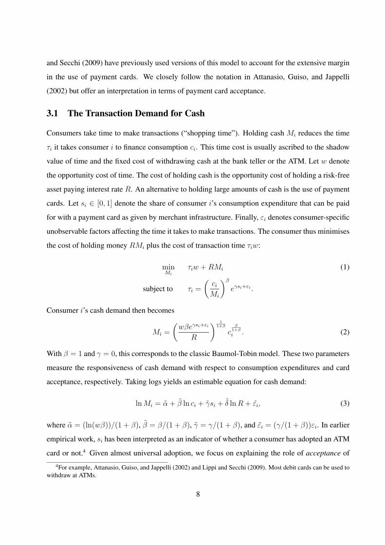
3.1 The Transaction Demand for Cash

Consumers take time to make transactions (“shopping time”). Holding cash Mi reduces the time

τi it takes consumer i to finance consumption ci. This time cost is usually ascribed to the shadow

value of time and the fixed cost of withdrawing cash at the bank teller or the ATM. Let w denote

the opportunity cost of time. The cost of holding cash is the opportunity cost of holding a risk-free

asset paying interest rate R. An alternative to holding large amounts of cash is the use of payment

cards. Let si ∈ [0, 1] denote the share of consumer i’s consumption expenditure that can be paid

for with a payment card as given by merchant infrastructure. Finally, εi denotes consumer-specific

unobservable factors affecting the time it takes to make transactions. The consumer thus minimises

the cost of holding money RMi plus the cost of transaction time τiw:

minMi

τiw +RMi (1)

subject to τi =

(ciMi

)β

eγsi+εi .

Consumer i’s cash demand then becomes

Mi =

(wβeγsi+εi

R

) 11+β

cβ

1+β

i . (2)

With β = 1 and γ = 0, this corresponds to the classic Baumol-Tobin model. These two parameters

measure the responsiveness of cash demand with respect to consumption expenditures and card

acceptance, respectively. Taking logs yields an estimable equation for cash demand:

lnMi = α + β ln ci + γsi + δ lnR + εi, (3)

where α = (ln(wβ))/(1 + β), β = β/(1 + β), γ = γ/(1 + β), and εi = (γ/(1 + β))εi. In earlier

empirical work, si has been interpreted as an indicator of whether a consumer has adopted an ATM

card or not.4 Given almost universal adoption, we focus on explaining the role of acceptance of

4For example, Attanasio, Guiso, and Jappelli (2002) and Lippi and Secchi (2009). Most debit cards can be used towithdraw at ATMs.

8

these cards. We thus interpret si as a variable measuring whether a payment can be made with

cards.

Observe that the model treats si as exogenous to the consumer and we assume that si is given

by the consumer’s perception of a merchant’s adoption of a card payment terminal. If si were

indeed a costless option to the consumer, it would be optimal for consumers to get rid of cash as

quickly as possible and always use cards whenever cards are accepted. The evidence provided in

Table 1 shows that this is the case most of the time, but not always: consumers sometimes pay

with a card although they have enough cash.5 While we address the potential endogeneity of si

when estimating (3), we will not be able to point to the source that causes it. Consequently, we will

not provide a structural interpretation of the estimated acceptance coefficient in equation (3). We

will interpret the coefficient as a reduced form capturing both the payment infrastructure offered

by merchants as well as consumers’ perception thereof. Our identification strategy outlined below

will try to account for both supply-side effects (like the number of cash registers) as well as demand

effects (the payment behaviour of friends).

3.2 Estimating Cash Demand

Respondents in the surveys indicate whether cards were accepted at the POS for every transaction

they report. At the transaction level, si is an indicator variable; at the person level, it denotes

a continuous variable measuring the fraction of the individual’s payments in terms of value that

could have been made with a card. The goal of our empirical work is to quantify the impact of

acceptance si on cash demand Mi. Given that acceptance facilitates transactions with payment

cards, we expect a larger si to reduce cash demand. The first challenge we face in estimating

the cash demand equation (3) is the potential measurement error in acceptance si because of false

reporting by survey respondents, resulting in a bias towards zero and underestimating the impact of

acceptance on cash demand. The second challenge in estimating the cash demand equation is the

potential endogeneity of acceptance si itself: if consumers have a lot of cash on hand (for instance

because of unexpected free withdrawal opportunity as in Alvarez and Lippi (2009)), they may be

more likely to visit a store that does not accept cards. Similarly, consumers with no cash at hand

5We thank a referee for pointing this out; Alvarez and Lippi (2014) solve a related model where si is actually achoice.

9

will avoid a cash-only store. This would cause a negative correlation between acceptance si and

the error term εi, resulting in a downward bias in our estimate of the coefficient of interest. We will

address these issues by employing appropriate econometric methods at the individual level and at

the transaction level, respectively, in the following sections.

4 Individual-Level Cash Demand

To understand the cash demand Mi at the individual level i, we estimate the following relationship:

lnMi = α+ β ln ci + γsi +Xiλ+ εi. (4)

This corresponds to the cash demand equation (3), with the dependent variable measured in terms

of how much cash is held at the beginning of the diary. Consumption is the total amount of

expenditures over the diary collection period (ci), and the share of acceptance is the fraction of

time that payment cards are accepted for each transaction undertaken. Finally, a vector of con-

trol variables including socio-demographic information about individual i (gender, employment

status, age, household size), characteristics of the consumer’s transactions (i.e., sectoral composi-

tion, transaction value quartiles, time of day and day of the week variables), and information on

opportunity cost of cash is denoted as Xi.

The results are summarised in Table 3.6 Column (1) contains the ordinary least squares (OLS)

estimate of consumption: 0.265 and 0.105 for Austria and Canada, respectively. The larger Aus-

trian consumption elasticity reflects that Austria is still a more cash-intensive economy: consumers

hold more cash and pay with cash more often. As a robustness check, we also consider cash con-

sumption only in column (2). As expected, the estimated coefficient magnitude is higher at 0.387

and 0.265 for Austria and Canada, respectively. Adding acceptance as a regressor, columns (3) and

(4), has no noticeable effect on the consumption and cash consumption elasticity estimates them-

selves. However, the effect of acceptance is substantially smaller for cash consumption (and not

significant for Austria). This result further adds to the intuition that using only cash consumption

increases the estimate of the coefficient on consumption since it assumes that households pay for

consumption only with cash. Therefore, households are more sensitive to changes in consumption.

6For brevity, we suppress estimates for the control variables but provide the full set of NLIV estimates in AppendixTables A.2 and A.3. The rest of the results are available from the authors upon request.

10

Moreover, given that households pay only in cash, acceptance should not matter—which is what

we find.7

4.1 Endogeneity of Acceptance

The simple shopping-time model presented in Section 3 considered the share of transactions that

can be made with cash as entirely determined by the supply side. Respondents’ cash holdings

may not, however, only be affected by acceptance but rather their cash holdings may determine

whether they transact at high- or low-acceptance stores. For example, a respondent with low

cash holdings would care if the retailer accepts cards or not. In the cash consumption regression

reported in column (4) of Table 3, this decision is considered exogenous because all consumption

is done in cash. So, in column (5), we estimate a linear instrumental variable (IV) model and focus

on the issue of endogeneity of the acceptance variable. The empirical strategy relies on finding

instrument(s) that are correlated with acceptance but are not with individual cash holdings. The

ideal candidates for these instruments are physical characteristics of the POS as they are correlated

with acceptance but do not affect individual cash holdings.

The Canadian diary contains one such physical characteristic: the number of cash registers at

each transaction (as reported by respondents). These instruments were also used in Arango, Huynh,

and Sabetti (2014), who model the discrete choice of payment at the POS. For the individual-level

regressions, the instruments are person i’s share of stores with zero to two, three to six, and more

than six cash registers. As these instruments are shares and do not have a symmetric distribution,

we use a third-order polynomial, as suggested by Lewbel (1997) and Escanciano, Jacho-Chavez,

and Lewbel (2012), to capture higher-order moments that may affect measurement error and also

increases the number of instruments available. For Austria, these variables are not available and

we therefore use an alternative set of instruments: average acceptance in municipality in which

the respondent resides, payment behaviour of close friends and the share of shops with terminals,

derived from administrative data, see the variable list in Table A.1. The average acceptance in mu-

nicipality is calculated from transactions reported by respondents residing in the same municipality

as respondent i, leaving out respondent i’s response. The rationale for using information regarding

7Our cash consumption elasticity estimates of 0.387 for Austria and 0.265 for Canada are broadly in line with thoseof Lippi and Secchi (2009) for Italy (∼0.35).

11

the payment behaviour of close friends is that they usually shop in the same type of stores and

have a comparable consumption basket. We expect instruments measured at the municipality level

rather than at the person level not to perform as well as those used for Canada.

The IV estimates of column (5) in Table 3, depict a significant effect of endogeneity acceptance

as the point estimate decreases from -0.519 to -1.332 for Austria and from -0.596 to -1.259 for

Canada, respectively. The consumption estimate does not materially change. The major impact

of instrumenting for acceptance is that it increases the effect of acceptance on cash holdings. We

implement two Wald F -tests of weak instruments (see Cragg and Donald (1993) and Kleibergen

and Paap (2006)). There are no critical values for these weak instruments tests but we use the

tabulated test statistics calculated by Stock and Yogo (2005) and find that there is marginal evidence

of rejection of weak instruments in Austria and Canada. The linear IV estimate model works well

for Austria and Canada as the Hansen-Sargan tests of overidentification are not rejected. We next

address potential nonlinearities in the share of acceptance in the first-stage regressions.

4.2 Functional Form of Acceptance

The share of acceptance for respondents with zero or one is 0.01 and 0.36 in Austria and 0.09 and

0.33 for Canada. Therefore, a non-trivial share lies between zero and one; hence, the assumption

of linear IV may not be tenable. We therefore relax the functional form by employing a nonlinear

instrumental variables method and implement it in two steps. In the first step we model the share

of acceptance as a fractional logit, as suggested by Papke and Wooldridge (1996) and compute

the predicted shares (constrained between zero and one) and include them in a linear second-stage

regression. To address the generated regressor problem, we bootstrap the regression estimates 1000

times. For Canada, the effect of the nonlinearities slightly reduces the effects of both consumption

and acceptance (0.111 to 0.109 for consumption and from -1.259 to -1.161 for acceptance). For

Austria, only the consumption elasticity is slightly reduced.

5 Transaction-Level Cash Demand

The previous analysis focused on average behaviour over the period of the diary. This aggregation

necessarily implies that for each individual household the temporal pattern of cash balances and

12

payment choices is averaged out over the period of the diary. However, the payment diaries con-

tain observations at the transaction level: for each transaction we observe the transaction amount,

whether cards were accepted or not, as well as many other transaction characteristics. We have

also computed the stock of cash held at each transaction. The richness of these data is likely to

yield a more precise representation of the cash-holding acceptance nexus.

Column (1) in Table 4 contains an OLS estimate of the elasticity of cash demand with respect

to transaction amount (consumption) and acceptance. Both coefficients are statistically significant.

The consumption elasticities are 0.176 and 0.099 for Austria and Canada, respectively. Acceptance

is also statistically and economically important, with coefficients of -0.258 and -0.260 for Austria

and Canada, respectively. Column (2) utilizes instrumental variables to account for endogeneity

of acceptance. The instruments used are similar in the individual-level regression; for Austria

they are: average acceptance in municipality, payment behaviour of close friends and the share

of shops with terminals. The instruments for Canada are: a dummy indicating whether the store

has three to six cash registers and a dummy indicating whether the store has six or more cash

registers. For Canada, the instruments for acceptance variables at the transaction level are binary;

therefore, we cannot use polynomials. It is not surprising that the IV results for Canada are not

significant, since the binary nature of instruments causes a substantial increase in the standard

errors for the regression. For Austria, the consumption elasticity in column (2) is 0.229 and the

effect of acceptance is -1.177. The IV results from Canada illustrate the role of nonlinearities in

the acceptance variable that is being instrumented with binary variables. Therefore, it is necessary

to relax the linear functional form of transaction-level cash demand.

5.1 Endogenous Switching Regression

To address nonlinearities in the functional form, we estimate a cash demand equation using the

endogenous switching regression suggested by Maddala (1983). The cash demand can be classified

13

into two regimes, si = 1 if a card payment is accepted or zero otherwise:

si = 1 if γZi + ui > 0

si = 0 if γZi + ui ≤ 0

M0 : lnM0i = α0 + β0 ln c0i +X0iλ0 + ϵ0i, (5)

M1 : lnM1i = α1 + β1 ln c1i +X1iλ1 + ϵ1i.

Here, lnMji denotes the natural logarithm of the cash stock of respondent i before each transac-

tion, X0 and X1 are vectors of weakly exogenous variables, and β0 and β1 are the parameters of

interest.8 The error terms ui, ϵ0i and ϵ1i have a trivariate normal distribution, with mean vector

zero and a well-defined covariance matrix. For an implementation of this method, see Lokshin and

Sajaia (2006). The vector of control variables (Xi) includes socio-demographic (gender, employ-

ment status, age, household size) and POS (sectoral composition, transaction value quartiles, time

of day and day of the week variables) characteristics.9 For the regime equation variables (Zi) are

the observables (Xi) plus the exclusion restrictions. Again, the exclusion restrictions are the same

as in the linear IV in the individual-level regression.

The results indicate that there are two regimes and that the selection is significant as both

p-values are less than 0.01. For Austria, Regime 1 (or the acceptance state) has a consumption

elasticity of 0.159, while Regime 0 (or the non-acceptance state) has a consumption elasticity of

0.233. Qualitatively similar results occur for Canada, with 0.094 and 0.186 for Regime 1 and 0,

respectively. These results indicate that the nonlinearities plus the exclusion restrictions provide

identification for the model. The economic results of these elasticities state that when respondents

are in non-acceptance areas, their cash demand is more inelastic than in acceptance areas, thus con-

firming our earlier results now at the transaction level. Finally, the null hypothesis of no selection

is also rejected for both countries.

5.2 Counterfactual Cash Demand

The coefficient estimates of the switching show that there is a substantial effect of acceptance on

the elasticity of cash demand with respect to consumption. The well-identified model (5) of cash

8Again, these parameters are backed out from the point estimates of β0 and β1 according to equation (2).9Control variables are defined in Table A.1. For brevity, we suppress estimates for the control variables. They are

reported separately in Table A.4 for Austria and Table A.5 for Canada.

14

demand can be used to construct counterfactual analyses that will allow us to quantify level and

distributional effects of acceptance. Specifically, the counterfactual scenario we undertake is the

following. We have two types of consumers, acceptance-type (A or “urban dweller”) and non-

acceptance-type (NA or “villager”). The terms “urban dweller” and “villager” are used to indicate

that acceptance is related to the two regimes (conditional densities). Conditional cash demand can

be computed using

E(lnMCAj|si = CAj, Xi) = Xiβ0 + σCAj

ρCAj

f(γZi)

F (γZi), (6)

with card acceptance CAj ∈ {A,NA}.

Table 5 contains the means of three conditional distributions:

1. Baseline: the difference between “urban dwellers” and “villagers”.

2. A decrease in acceptance, i.e., an “urban dweller” who shops in a “village”.

3. An increase in acceptance, i.e., a “villager” who shops in the “city”.

These scenarios illustrate that the average difference between urban and villager cash demand

is about -19% and -23% for Austria and Canada, respectively. However, the effect of acceptance on

the types of respondents is quite asymmetric: increasing acceptance lowers cash demand by 32%

and 46% for Austria and Canada, respectively. However, decreasing acceptance increases cash

demand by -26% and -19% for Austria and Canada, respectively. To ensure that the results are not

just an artefact of the shape of the distributions, Figure 1 plots the entire counterfactual distributions

for the scenarios described. The densities in the acceptance regime are red (light grey), and the

densities in the non-acceptance regime are green (dark grey). Again, a uniform picture emerges

for both Austria and Canada. In the acceptance regime the distribution is centred at lower values

and exhibits much lower variation than in the non-acceptance regime (top panels of Figure 1). The

non-acceptance regime is characterized by a centre at higher values and a substantial right tail, even

for “urban dwellers”. This result is consistent with the presence of substantial lumpy purchases

that have to be paid for in cash. Again, moving the “villager” to the acceptance regime has a more

pronounced effect on cash holding (middle panels of Figure 1) than moving an “urban dweller” to

the non-acceptance regime (bottom panels of Figure 1).

15

These estimates have a strong prediction for the potential evolution of cash. As more POS

terminals are installed, cash demand will decrease. In addition to this level effect of acceptance

on cash demand, we found a substantially smaller consumption elasticity in the acceptance regime

(see Table 4). This suggests that an increase in card acceptance will increase the velocity of cash,

i.e., cash is withdrawn and spent immediately. As we move to the extreme case of universal

acceptance, the velocity of cash would become infinite and both the level of cash demand and the

consumption elasticity would approach zero.10

We are not in this extreme world yet as the adoption of retail payment innovations is still

speculative; see Fung, Huynh, and Sabetti (2012) or Chen, Felt, and Huynh (2014). Our results

suggest that cash still has a precautionary component, i.e., it serves as a buffer for the possibility

of non-acceptance. The asymmetry of the effect of acceptance suggests that the precautionary

nature is dominated by the supply-side effect of increased acceptance. There is also an element of

consumer-driven preferences, especially for small-value transactions, as suggested by Wakamori

and Welte (2013).

5.3 Opportunity Cost of Cash

We next examine how the opportunity cost of holding cash affects cash demand. Earlier studies

mostly rely on cross-sectional or intertemporal variation in the nominal interest rate to measure

the opportunity cost. Given the short time horizons of the surveys (three and seven days), and the

absence of cross-sectional variation in deposit rates in Austria and Canada, an alternative measure

is needed to proxy for the opportunity costs of cash. Alvarez and Lippi (2009) use crime statistics

as a proxy for the probability of being robbed. Both the Austrian and the Canadian surveys contain

subjective variables that are related to the risk of being robbed.

In the Austrian survey, a question asked the amount of cash in the pocket that causes respon-

dents to feel uncomfortable. This variable, called risk of theft, is then mapped into a continuous

probability (from 0 to 1). The risk of theft variable in Canada asked respondents about their per-

ception, on a scale of 1 (very unlikely) to 5 (very likely), about the probability of losing $20. This

variable does not match well with the Austrian risk of theft variable since it is not a continuous10We thank a referee for alerting us to this mechanism. Alvarez, Guiso, and Lippi (2012) illustrate this mechanism

in the context of durable goods purchases, where the liquid assets required to purchase durable goods are withdrawnand spent immediately.

16

variable, as the question only pertains to the likelihood of losing a rather trivial amount. Another

possible reason is that Canadian respondents hold less cash than Austrians. Consequently, it is not

suitable as a proxy for the opportunity cost of cash. Instead, we follow the suggestion of Briglevics

and Schuh (2013) to focus on respondents who do not pay the complete balance of their credit card

statement at the due date and therefore incur interest charges, commonly known as revolvers. In

their study, they find that revolvers are a good proxy for interest-elastic respondents since when

they face low cash balances and need to use cards they must weigh the benefits of using a payment

card with the incurred cost of interest. Almost half of the sample of respondents (and transactions)

in Canada are revolvers.

The results in Table A.4 show the effect of risk of theft for Austria. In the acceptance regime

the coefficient is -0.150 but insignificant, while it is -0.349 in the non-acceptance regime and

significant. This highlights that when card payments are accepted the sensitivity to risk of theft of

cash is lower since there is less need to use or hold cash. The results in Table A.5 show that in

the acceptance regime the coefficient on revolving is -0.180 while in the non-acceptance regime

it is -0.122. Both coefficients are significantly different from zero, but we cannot reject the null

hypothesis of them being equal. It shows that when the opportunity cost of holding cash is high,

consumers become even more careful in managing their cash balances and keep them low. The

results highlight the use of these (imperfect) proxies for the opportunity cost of holding cash.

6 Conclusions

This paper analyses how consumers manage their cash balances if they are uncertain whether pay-

ment cards will be accepted. We adapt the stylized Baumol-Tobin cash inventory model to account

for card acceptance. We derive and estimate the resulting cash demand using payment diary data

from Austria and Canada. Our estimation procedure accounts for endogeneity, nonlinearities and

aggregation. We find that the extended Baumol-Tobin model yields robust results across countries.

Acceptance of payment cards has a strong impact on cash balances when all consumption expendi-

tures are considered rather than only cash consumption, as in Lippi and Secchi (2009) and Alvarez

and Lippi (2009).

Accounting for acceptance and its endogeneity implies smaller consumption elasticities than

17

predicted by the Baumol-Tobin model. We show that consumers behave differently depending on

whether they (choose to) shop in an environment where cards are accepted versus whether cards

are not accepted. Acceptance reduces both the level of cash demand and the transaction elasticity

of cash demand. Our counterfactuals show that increased acceptance would strongly reduce cash

demand. Cash demand in environments where cards are not accepted is driven partly by precau-

tionary motives or infrequent lumpy purchases that are paid for in cash. We thus conclude that

pushing for increased acceptance will further reduce cash holdings, but not entirely eliminate them

in part because of the precautionary motives but also because of the preference of some consumers

for using cash, as discussed in Wakamori and Welte (2013) and von Kalckreuth, Schmidt, and Stix

(2014).

ReferencesALVAREZ, F., L. GUISO, AND F. LIPPI (2012): “Durable Consumption and Asset Management

with Transaction and Observation Costs,” American Economic Review, 102(5), 2272–2300.

ALVAREZ, F., AND F. LIPPI (2009): “Financial Innovation and the Transactions Demand forCash,” Econometrica, 77(2), 363–402.

(2013): “The Demand of Liquid Assets with Uncertain Lumpy Expenditures,” Journal ofMonetary Economics, 60, 753–770.

(2014): “Cash Burns,” mimeo.

AMROMIN, G., AND S. CHAKRAVORTI (2009): “Whither Loose Change? The Diminishing De-mand for Small-Denomination Currency,” Journal of Money, Credit and Banking, 41(2-3), 315–335.

ARANGO, C., K. HUYNH, AND L. SABETTI (2014): “Consumer Payment Choice: Merchant CardAcceptance versus Pricing Incentives,” .

ATTANASIO, O. R., L. GUISO, AND T. JAPPELLI (2002): “The Demand for Money, FinancialInnovation, and the Welfare Cost of Inflation: An Analysis with Household Data,” Journal ofPolitical Economy, 110(2), 317–351.

BAGNALL, J., D. BOUNIE, K. HUYNH, A. KOSSE, T. SCHMIDT, S. SCHUH, AND H. STIX

(2014): “Consumer Cash Usage: A Cross-Country Comparison with Payment Diary SurveyData,” Working Papers 14-20, Bank of Canada.

BAR-ILAN, A., AND N. MARION (2013): “Demand for Cash with Intra-period Endogenous Con-sumption,” Journal of Economic Dynamics and Control, 37(12), 2668–2678.

18

BAUMOL, W. J. (1952): “The Transactions Demand for Cash: An Inventory Theoretic Approach,”The Quarterly Journal of Economics, pp. 545–556.

BOUHDAOUI, Y., AND D. BOUNIE (2012): “Modeling the Share of Cash Payments in the Econ-omy: An Application to France,” International Journal of Central Banking.

BRIGLEVICS, T., AND S. SCHUH (2013): “U.S. Consumer Demand for Cash in the Era of Low In-terest Rates and Electronic Payments,” Working Papers 13-23, Federal Reserve Bank of Boston.

CAMERA, G., M. CASARI, AND S. BORTOLOTTI (2014): “An Experiment on Retail PaymentsSystems,” SAFE Working Paper Series 49, Research Center SAFE - Sustainable Architecturefor Finance in Europe, Goethe University Frankfurt.

CHEN, H., M.-H. FELT, AND K. HUYNH (2014): “Retail Payment Innovations and Cash Usage:Accounting for Attrition Using Refreshment Samples,” Working Papers 14-27, Bank of Canada.

CRAGG, J. G., AND S. G. DONALD (1993): “Testing Identifiability and Specification in Instru-mental Variable Models,” Econometric Theory, 9(02), 222–240.

ESCANCIANO, J. C., D. T. JACHO-CHAVEZ, AND A. LEWBEL (2012): “Identification and Esti-mation of Semiparametric Two Step Models,” .

FUNG, B., K. HUYNH, AND L. SABETTI (2012): “The Impact of Retail Payment Innovations onCash Usage,” Working Papers 12-14, Bank of Canada.

HUMPHREY, D., M. WILLESSON, T. LINDBLOM, AND G. BERGENDAHL (2003): “What Does ItCost to Make a Payment?,” Review of Network Economics, 2(2).

KLEIBERGEN, F., AND R. PAAP (2006): “Generalized Reduced Rank Tests Using the SingularValue Decomposition,” Journal of Econometrics, 133(1), 97–126.

LEWBEL, A. (1997): “Constructing Instruments for Regressions with Measurement Error when noAdditional Data are Available, with an Application to Patents and R&D,” Econometrica, 65(5),1201–1214.

LIPPI, F., AND A. SECCHI (2009): “Technological Change and the Households’ Demand forCurrency,” Journal of Monetary Economics, 56(2), 222–230.

LOKSHIN, M., AND Z. SAJAIA (2006): “MOVESTAY: Stata Module for Maximum LikelihoodEstimation of Endogenous Regression Switching Models,” Statistical Software Components,Boston College Department of Economics.

MADDALA, G. (1983): Limited Dependent and Qualitative Variables in Econometrics. CambridgeUniversity Press.

MASTERS, A., AND L. R. RODRIGUEZ-REYES (2005): “Endogenous Credit-Card Acceptance ina Model of Precautionary Demand for Money,” Oxford Economic Papers, 57(1), 157–168.

19

MCCALLUM, B., AND M. S. GOODFRIEND (1987): “Money: Theoretical Analysis of the Demandfor Money,” in The New Palgrave: A Dictionary of Economic Theory and Doctrine, ed. byJ. Eatwell, P. Newman, and M. Milgate. The Macmillan Press, London, first edn.

MULLIGAN, C. B., AND X. SALA-I-MARTIN (2000): “Extensive Margins and the Demand forMoney at Low Interest Rates,” Journal of Political Economy, 108(5), 961–991.

PAPKE, L. E., AND J. M. WOOLDRIDGE (1996): “Econometric Methods for Fractional ResponseVariables with an Application to 401(K) Plan Participation Rates,” Journal of Applied Econo-metrics, 11(6), 619–632.

SCHMIEDEL, H., G. KOSTOVA, AND W. RUTTENBERG (2012): “The Social and Private Costs ofRetail Payment Instruments: A European Perspective,” ECB Occasional Paper, (137).

SEGENDORF, B. L., AND T. JANSSON (2012): “The Cost of Consumer Payments in Sweden,”Riksbank Research Paper Series, (93).

STOCK, J., AND M. YOGO (2005): “Testing for Weak Instruments in Linear IV Regression,” inIdentification and Inference for Econometric Models: Essays in Honor of Thomas Rothenberg,ed. by D. W. K. Andrews, and J. H. Stock, chap. 6, pp. 80–108. Cambridge University Press,Cambridge, first edn.

TOBIN, J. (1956): “The Interest-Elasticity of Transactions Demand for Cash,” The Review ofEconomics and Statistics, 38(3), 241–247.

VON KALCKREUTH, U., T. SCHMIDT, AND H. STIX (2014): “Using Cash to Monitor Expendi-tures - Implications for Payments, Currency Demand and Withdrawal Behavior,” forthcomingJournal of Money, Credit and Banking.

WAKAMORI, N., AND A. WELTE (2013): “Why Do Shoppers Use Cash? Evidence from ShoppingDiary Data,” Discussion Paper Series of SFB/TR 15 Governance and the Efficiency of EconomicSystems 431, Free University of Berlin, Humboldt University of Berlin, University of Bonn,University of Mannheim, University of Munich.

WHITESELL, W. C. (1989): “The Demand for Currency versus Debitable Accounts: A Note,”Journal of Money, Credit and Banking, 21(2), 246–57.

20

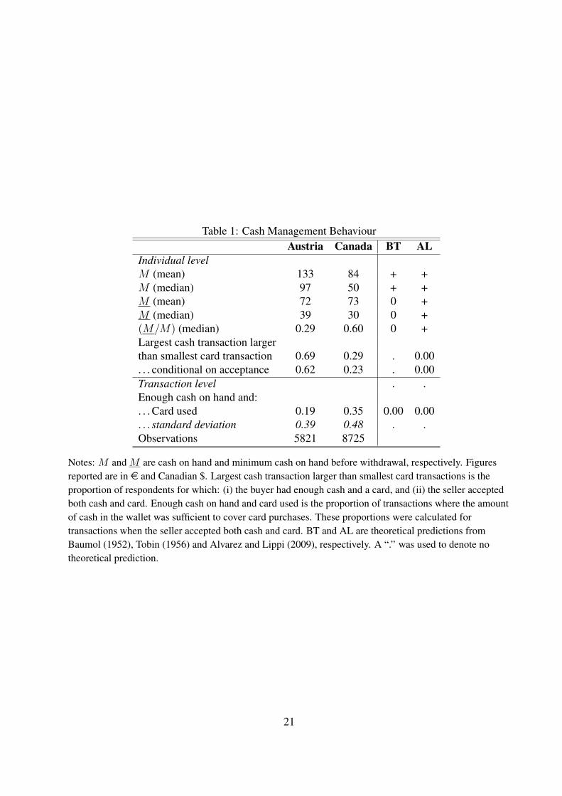
Table 1: Cash Management BehaviourAustria Canada BT AL

Individual levelM (mean) 133 84 + +M (median) 97 50 + +M (mean) 72 73 0 +M (median) 39 30 0 +(M/M) (median) 0.29 0.60 0 +Largest cash transaction largerthan smallest card transaction 0.69 0.29 . 0.00. . . conditional on acceptance 0.62 0.23 . 0.00Transaction level . .Enough cash on hand and:. . . Card used 0.19 0.35 0.00 0.00. . . standard deviation 0.39 0.48 . .Observations 5821 8725

Notes: M and M are cash on hand and minimum cash on hand before withdrawal, respectively. Figuresreported are in e and Canadian $. Largest cash transaction larger than smallest card transactions is theproportion of respondents for which: (i) the buyer had enough cash and a card, and (ii) the seller acceptedboth cash and card. Enough cash on hand and card used is the proportion of transactions where the amountof cash in the wallet was sufficient to cover card purchases. These proportions were calculated fortransactions when the seller accepted both cash and card. BT and AL are theoretical predictions fromBaumol (1952), Tobin (1956) and Alvarez and Lippi (2009), respectively. A “.” was used to denote notheoretical prediction.

21

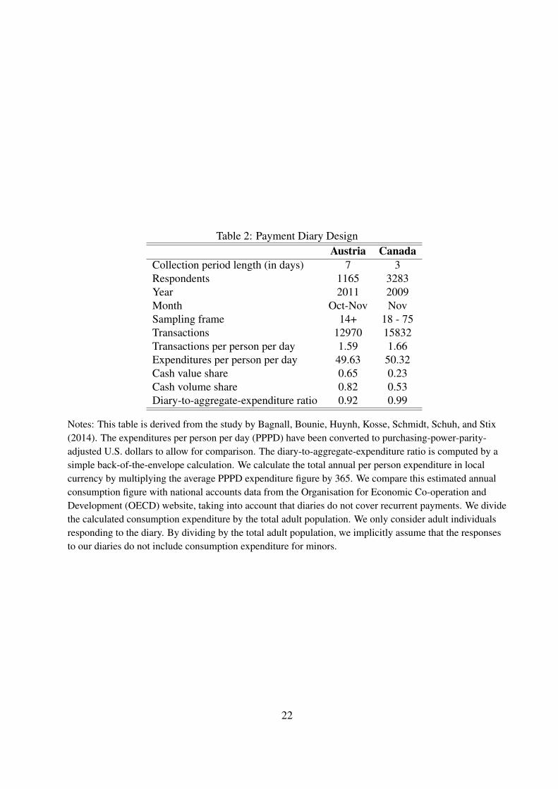
Table 2: Payment Diary DesignAustria Canada

Collection period length (in days) 7 3Respondents 1165 3283Year 2011 2009Month Oct-Nov NovSampling frame 14+ 18 - 75Transactions 12970 15832Transactions per person per day 1.59 1.66Expenditures per person per day 49.63 50.32Cash value share 0.65 0.23Cash volume share 0.82 0.53Diary-to-aggregate-expenditure ratio 0.92 0.99

Notes: This table is derived from the study by Bagnall, Bounie, Huynh, Kosse, Schmidt, Schuh, and Stix(2014). The expenditures per person per day (PPPD) have been converted to purchasing-power-parity-adjusted U.S. dollars to allow for comparison. The diary-to-aggregate-expenditure ratio is computed by asimple back-of-the-envelope calculation. We calculate the total annual per person expenditure in localcurrency by multiplying the average PPPD expenditure figure by 365. We compare this estimated annualconsumption figure with national accounts data from the Organisation for Economic Co-operation andDevelopment (OECD) website, taking into account that diaries do not cover recurrent payments. We dividethe calculated consumption expenditure by the total adult population. We only consider adult individualsresponding to the diary. By dividing by the total adult population, we implicitly assume that the responsesto our diaries do not include consumption expenditure for minors.

22

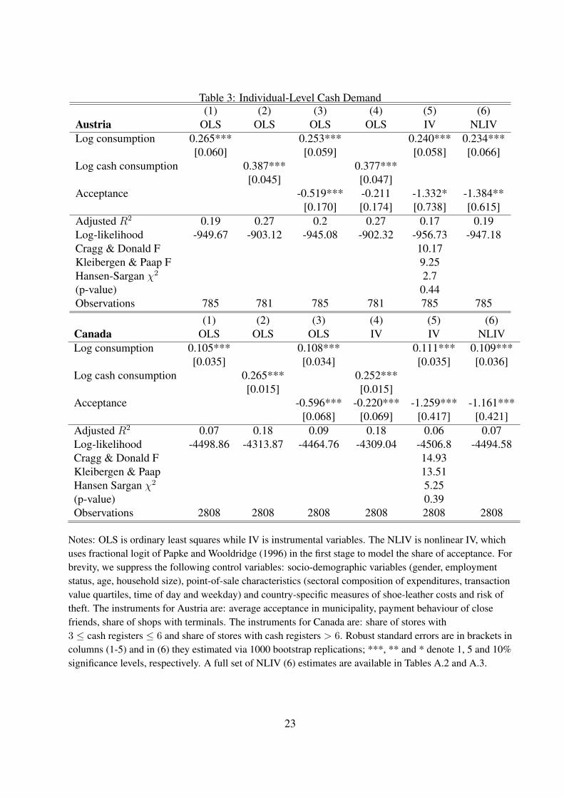
Table 3: Individual-Level Cash Demand(1) (2) (3) (4) (5) (6)

Austria OLS OLS OLS OLS IV NLIVLog consumption 0.265*** 0.253*** 0.240*** 0.234***

[0.060] [0.059] [0.058] [0.066]Log cash consumption 0.387*** 0.377***

[0.045] [0.047]Acceptance -0.519*** -0.211 -1.332* -1.384**

[0.170] [0.174] [0.738] [0.615]Adjusted R2 0.19 0.27 0.2 0.27 0.17 0.19Log-likelihood -949.67 -903.12 -945.08 -902.32 -956.73 -947.18Cragg & Donald F 10.17Kleibergen & Paap F 9.25Hansen-Sargan χ2 2.7(p-value) 0.44Observations 785 781 785 781 785 785

(1) (2) (3) (4) (5) (6)Canada OLS OLS OLS IV IV NLIVLog consumption 0.105*** 0.108*** 0.111*** 0.109***

[0.035] [0.034] [0.035] [0.036]Log cash consumption 0.265*** 0.252***

[0.015] [0.015]Acceptance -0.596*** -0.220*** -1.259*** -1.161***

[0.068] [0.069] [0.417] [0.421]Adjusted R2 0.07 0.18 0.09 0.18 0.06 0.07Log-likelihood -4498.86 -4313.87 -4464.76 -4309.04 -4506.8 -4494.58Cragg & Donald F 14.93Kleibergen & Paap 13.51Hansen Sargan χ2 5.25(p-value) 0.39Observations 2808 2808 2808 2808 2808 2808

Notes: OLS is ordinary least squares while IV is instrumental variables. The NLIV is nonlinear IV, whichuses fractional logit of Papke and Wooldridge (1996) in the first stage to model the share of acceptance. Forbrevity, we suppress the following control variables: socio-demographic variables (gender, employmentstatus, age, household size), point-of-sale characteristics (sectoral composition of expenditures, transactionvalue quartiles, time of day and weekday) and country-specific measures of shoe-leather costs and risk oftheft. The instruments for Austria are: average acceptance in municipality, payment behaviour of closefriends, share of shops with terminals. The instruments for Canada are: share of stores with3 ≤ cash registers ≤ 6 and share of stores with cash registers > 6. Robust standard errors are in brackets incolumns (1-5) and in (6) they estimated via 1000 bootstrap replications; ***, ** and * denote 1, 5 and 10%significance levels, respectively. A full set of NLIV (6) estimates are available in Tables A.2 and A.3.

23

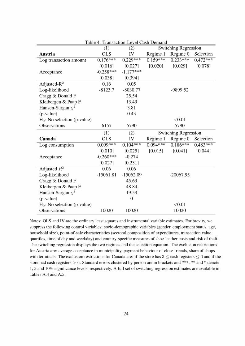
Table 4: Transaction-Level Cash Demand(1) (2) Switching Regression

Austria OLS IV Regime 1 Regime 0 SelectionLog transaction amount 0.176*** 0.229*** 0.159*** 0.233*** 0.472***

[0.016] [0.027] [0.020] [0.029] [0.078]Acceptance -0.258*** -1.177***

[0.038] [0.394]Adjusted-R2 0.16 0.05Log-likelihood -8123.7 -8030.77 -9899.52Cragg & Donald F 25.54Kleibergen & Paap F 13.49Hansen-Sargan χ2 3.81(p-value) 0.43H0: No selection (p-value) <0.01Observations 6157 5790 5790

(1) (2) Switching RegressionCanada OLS IV Regime 1 Regime 0 SelectionLog consumption 0.099*** 0.104*** 0.094*** 0.186*** 0.483***

[0.010] [0.025] [0.015] [0.041] [0.044]Acceptance -0.260*** -0.274

[0.027] [0.231]Adjusted R2 0.06 0.06Log-likelihood -15061.81 -15062.09 -20067.95Cragg & Donald F 45.69Kleibergen & Paap F 48.84Hansen-Sargan χ2 19.59(p-value) 0H0: No selection (p-value) <0.01Observations 10020 10020 10020

Notes: OLS and IV are the ordinary least squares and instrumental variable estimates. For brevity, wesuppress the following control variables: socio-demographic variables (gender, employment status, age,household size), point-of-sale characteristics (sectoral composition of expenditures, transaction valuequartiles, time of day and weekday) and country-specific measures of shoe-leather costs and risk of theft.The switching regression displays the two regimes and the selection equation. The exclusion restrictionsfor Austria are: average acceptance in municipality, payment behaviour of close friends, share of shopswith terminals. The exclusion restrictions for Canada are: if the store has 3 ≤ cash registers ≤ 6 and if thestore had cash registers > 6. Standard errors clustered by person are in brackets and ***, ** and * denote1, 5 and 10% significance levels, respectively. A full set of switching regression estimates are available inTables A.4 and A.5.

24

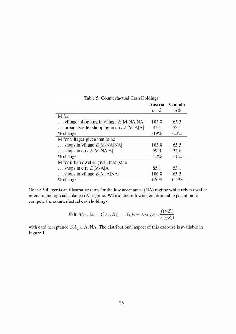
Table 5: Counterfactual Cash HoldingsAustria Canada

in e in $M for. . . villager shopping in village E[M-NA|NA] 105.8 65.5. . . urban dweller shopping in city E[M-A|A] 85.1 53.1% change -19% -23%M for villager given that (s)he. . . shops in village E[M-NA|NA] 105.8 65.5. . . shops in city E[M-NA|A] 69.9 35.6% change -32% -46%M for urban dweller given that (s)he. . . shops in city E[M-A|A] 85.1 53.1. . . shops in village E[M-A|NA] 106.8 63.5% change +26% +19%

Notes: Villager is an illustrative term for the low acceptance (NA) regime while urban dwellerrefers to the high acceptance (A) regime. We use the following conditional expectation tocompute the counterfactual cash holdings:

E(lnMCAj|si = CAj, Xi) = Xiβ0 + σCAj

ρCAj

f(γZi)

F (γZi)

with card acceptance CAj ∈ A, NA. The distributional aspect of this exercise is available inFigure 1.

25

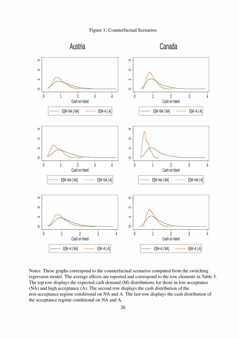
Figure 1: Counterfactual Scenarios

01

23

0 1 2 3 4Cash on Hand

E[M−NA | NA] E[M−A | A]

01

23

0 1 2 3 4Cash on Hand

E[M−NA | NA] E[M−NA | A]

01

23

0 1 2 3 4Cash on Hand

E[M−A | NA] E[M−A | A]

Austria

01

23

0 1 2 3 4Cash on Hand

E[M−NA | NA] E[M−A | A]

01

23

0 1 2 3 4Cash on Hand

E[M−NA | NA] E[M−NA | A]

01

23

0 1 2 3 4Cash on Hand

E[M−A | NA] E[M−A | A]

Canada

Notes: These graphs correspond to the counterfactual scenarios computed from the switchingregression model. The average effects are reported and correspond to the row elements in Table 5.The top row displays the expected cash demand (M) distributions for those in low acceptance(NA) and high acceptance (A). The second row displays the cash distribution of thenon-acceptance regime conditional on NA and A. The last row displays the cash distribution ofthe acceptance regime conditional on NA and A.

26

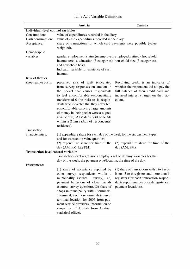
Table A.1: Variable Definitions

Austria CanadaIndividual-level control variablesConsumption: value of expenditures recorded in the diary.Cash consumption: value of cash expenditures recorded in the diary.Acceptance: share of transactions for which card payments were possible (value

weighted).Demographicvariables: gender, employment status (unemployed, employed, retired), household

income tercils, education (3 categories), household size (3 categories),and household head.Indicator variable for existence of cashincome.

Risk of theft orshoe-leather costs: perceived risk of theft (calculated

from survey responses on amount inthe pocket that causes respondentsto feel uncomfortable (exponentiallytransformed 0 (no risk) to 1; respon-dents who indicated that they never feeluncomfortable carrying large amountsof money in their pocket were assigneda value of 0), ATM density (# of ATMswithin a 2 km radius of respondents’residence).

Revolving credit is an indicator ofwhether the respondent did not pay thefull balance of their credit card andincurred interest charges on their ac-count.

Transactioncharacteristics: (1) expenditure share for each day of the week for the six payment types

and for transaction value quartiles;(2) expenditure share for time of theday (AM, PM, late PM).

(2) expenditure share for time of theday (AM, PM).

Transaction-level control variablesTransaction-level regressions employ a set of dummy variables for theday of the week, the payment type/location, the time of the day.

Instruments(1) share of acceptance reported byother survey respondents within amunicipality (source: survey), (2)payment behaviour of close friends(source: survey question), (3) share ofshops in muncipality with 0 terminals,1 terminal, 2 or more terminals (source:terminal location for 2005 from pay-ment service providers, information onshops from 2011 data from Austrianstatistical office).

(1) share of transactions with 0 to 2 reg-isters, 3 to 6 registers and more than 6registers (for each transaction respon-dents report number of cash registers atpayment locations).

27

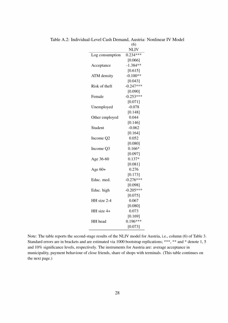
Table A.2: Individual-Level Cash Demand, Austria: Nonlinear IV Model(6)

NLIVLog consumption 0.234***

[0.066]Acceptance -1.384**

[0.615]ATM density -0.100**

[0.043]Risk of theft -0.247***

[0.090]Female -0.253***

[0.071]Unemployed -0.078

[0.148]Other employed 0.044

[0.146]Student -0.062

[0.164]Income Q2 0.052

[0.080]Income Q3 0.166*

[0.097]Age 36-60 0.137*

[0.081]Age 60+ 0.276

[0.173]Educ. med. -0.276***

[0.098]Educ. high -0.205***

[0.075]HH size 2-4 0.067

[0.080]HH size 4+ 0.073

[0.169]HH head 0.196***

[0.073]

Note: The table reports the second-stage results of the NLIV model for Austria, i.e., column (6) of Table 3.Standard errors are in brackets and are estimated via 1000 bootstrap replications; ***, ** and * denote 1, 5and 10% significance levels, respectively. The instruments for Austria are: average acceptance inmunicipality, payment behaviour of close friends, share of shops with terminals. (This table continues onthe next page.)

28

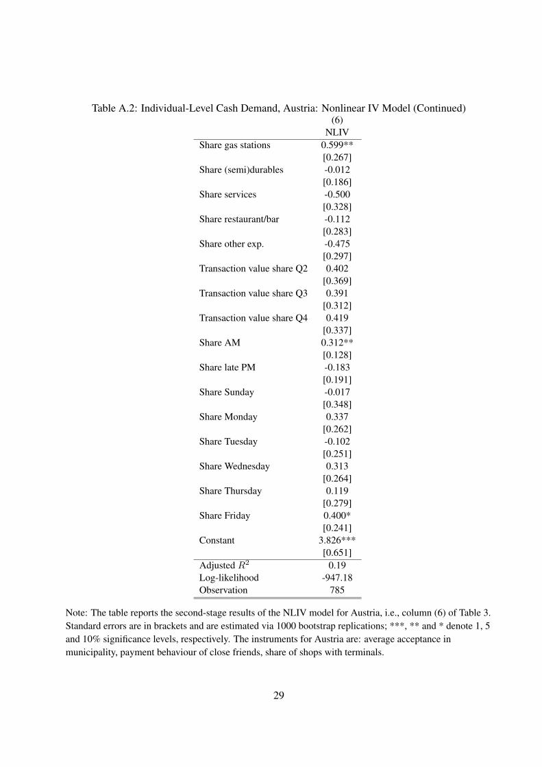
Table A.2: Individual-Level Cash Demand, Austria: Nonlinear IV Model (Continued)(6)

NLIVShare gas stations 0.599**

[0.267]Share (semi)durables -0.012

[0.186]Share services -0.500

[0.328]Share restaurant/bar -0.112

[0.283]Share other exp. -0.475

[0.297]Transaction value share Q2 0.402

[0.369]Transaction value share Q3 0.391

[0.312]Transaction value share Q4 0.419

[0.337]Share AM 0.312**

[0.128]Share late PM -0.183

[0.191]Share Sunday -0.017

[0.348]Share Monday 0.337

[0.262]Share Tuesday -0.102

[0.251]Share Wednesday 0.313

[0.264]Share Thursday 0.119

[0.279]Share Friday 0.400*

[0.241]Constant 3.826***

[0.651]Adjusted R2 0.19Log-likelihood -947.18Observation 785

Note: The table reports the second-stage results of the NLIV model for Austria, i.e., column (6) of Table 3.Standard errors are in brackets and are estimated via 1000 bootstrap replications; ***, ** and * denote 1, 5and 10% significance levels, respectively. The instruments for Austria are: average acceptance inmunicipality, payment behaviour of close friends, share of shops with terminals.

29

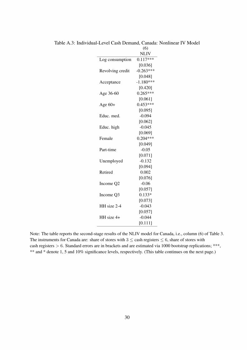
Table A.3: Individual-Level Cash Demand, Canada: Nonlinear IV Model(6)

NLIVLog consumption 0.117***

[0.036]Revolving credit -0.263***

[0.048]Acceptance -1.180***

[0.420]Age 36-60 0.265***

[0.061]Age 60+ 0.453***

[0.095]Educ. med. -0.094

[0.062]Educ. high -0.045

[0.069]Female 0.204***

[0.049]Part-time -0.05

[0.071]Unemployed -0.132

[0.094]Retired 0.002

[0.076]Income Q2 -0.06

[0.057]Income Q3 0.133*

[0.073]HH size 2-4 -0.043

[0.057]HH size 4+ -0.044

[0.111]

Note: The table reports the second-stage results of the NLIV model for Canada, i.e., column (6) of Table 3.The instruments for Canada are: share of stores with 3 ≤ cash registers ≤ 6, share of stores withcash registers > 6. Standard errors are in brackets and are estimated via 1000 bootstrap replications; ***,** and * denote 1, 5 and 10% significance levels, respectively. (This table continues on the next page.)

30

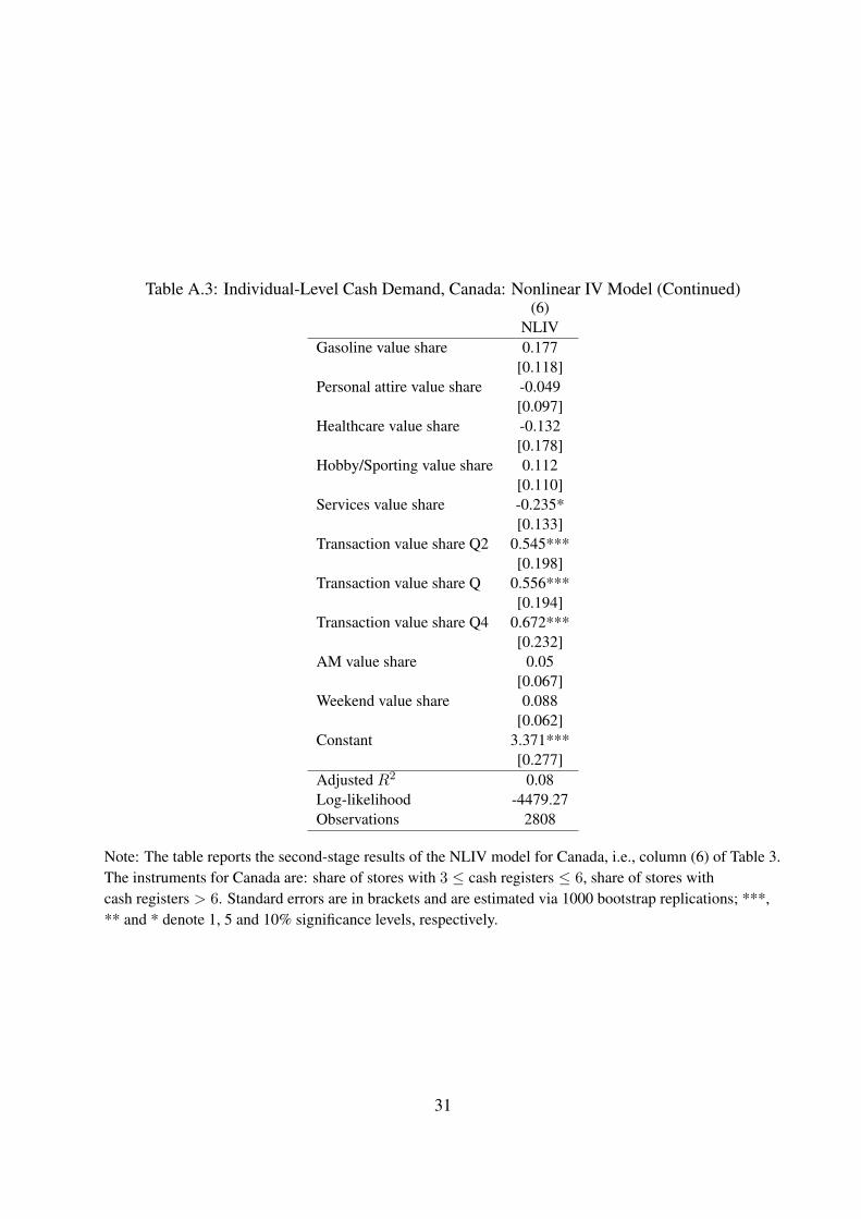
Table A.3: Individual-Level Cash Demand, Canada: Nonlinear IV Model (Continued)(6)

NLIVGasoline value share 0.177

[0.118]Personal attire value share -0.049

[0.097]Healthcare value share -0.132

[0.178]Hobby/Sporting value share 0.112

[0.110]Services value share -0.235*

[0.133]Transaction value share Q2 0.545***

[0.198]Transaction value share Q 0.556***

[0.194]Transaction value share Q4 0.672***

[0.232]AM value share 0.05

[0.067]Weekend value share 0.088

[0.062]Constant 3.371***

[0.277]Adjusted R2 0.08Log-likelihood -4479.27Observations 2808

Note: The table reports the second-stage results of the NLIV model for Canada, i.e., column (6) of Table 3.The instruments for Canada are: share of stores with 3 ≤ cash registers ≤ 6, share of stores withcash registers > 6. Standard errors are in brackets and are estimated via 1000 bootstrap replications; ***,** and * denote 1, 5 and 10% significance levels, respectively.

31

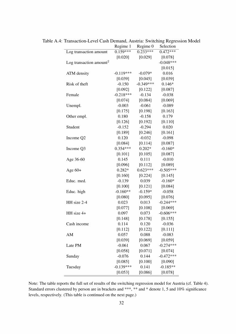
Table A.4: Transaction-Level Cash Demand, Austria: Switching Regression ModelRegime 1 Regime 0 Selection

Log transaction amount 0.159*** 0.233*** 0.472***[0.020] [0.029] [0.078]

Log transaction amount2 -0.048***[0.015]

ATM density -0.119*** -0.079* 0.016[0.039] [0.045] [0.039]

Risk of theft -0.150 -0.349*** 0.146*[0.092] [0.122] [0.087]

Female -0.218*** -0.134 -0.038[0.074] [0.084] [0.069]

Unempl. -0.003 -0.061 -0.089[0.175] [0.198] [0.163]

Other empl. 0.180 -0.158 0.179[0.126] [0.192] [0.110]

Student -0.152 -0.294 0.020[0.189] [0.246] [0.161]

Income Q2 0.120 -0.032 -0.098[0.084] [0.114] [0.087]

Income Q3 0.354*** 0.202* -0.160*[0.101] [0.105] [0.087]

Age 36-60 0.145 0.111 -0.010[0.096] [0.112] [0.089]

Age 60+ 0.282* 0.623*** -0.505***[0.160] [0.224] [0.145]

Educ. med. -0.139 0.039 -0.160*[0.100] [0.121] [0.084]

Educ. high -0.160** -0.159* -0.058[0.080] [0.095] [0.076]

HH size 2-4 0.023 0.013 -0.244***[0.077] [0.108] [0.069]

HH size 4+ 0.097 0.073 -0.606***[0.148] [0.178] [0.155]

Cash income 0.114 0.120 -0.036[0.112] [0.122] [0.111]

AM 0.057 0.088 -0.083[0.039] [0.069] [0.059]

Late PM -0.061 0.067 -0.274***[0.058] [0.071] [0.074]

Sunday -0.076 0.144 -0.472***[0.085] [0.100] [0.090]

Tuesday -0.139*** 0.141 -0.185**[0.053] [0.086] [0.078]

Note: The table reports the full set of results of the switching regression model for Austria (cf. Table 4).Standard errors clustered by person are in brackets and ***, ** and * denote 1, 5 and 10% significancelevels, respectively. (This table is continued on the next page.)

32

Table A.4: Transaction-Level Cash Demand, Austria: Switching Regression Model (Continued)Regime 1 Regime 0 Selection

Wednesday -0.116** 0.046 -0.144*[0.057] [0.090] [0.075]

Thursday -0.115** 0.076 -0.118[0.058] [0.100] [0.077]

Friday -0.106* -0.039 -0.128*[0.059] [0.104] [0.077]

Saturday -0.153*** -0.002 -0.103[0.057] [0.101] [0.080]

Typical week 0.037 0.070 0.209***[0.087] [0.084] [0.070]

Gas stations 0.646***[0.165]

(Semi)durables 0.125[0.088]

Services -1.009***[0.102]

Restaurant/bar -1.515***[0.079]

Other expenses -0.862***[0.088]

Friends use less cash -0.129*[0.070]

Acceptance neighbours 1.193***[0.311]

Share shops 1 terminal -1.254***[0.320]

Share shops >1 terminal 3.160***[0.940]

Constant 3.954*** 3.981*** 0.014[0.162] [0.192] [0.347]

Log σ -0.081** -0.156***[0.037] [0.047]

ρ 0.124** -0.065[0.063] [0.086]

H0: No selection 1824.11(p-value) 0.000H0: β0 = β1 5.36(p-value) 0.021Log-likelihood -9899.52Observations 5790Persons 739

Note: The table reports the full set of results of the switching regression model for Austria (cf. Table 4).Standard errors clustered by person are in brackets and ***, ** and * denote 1, 5 and 10% significancelevels, respectively.

33

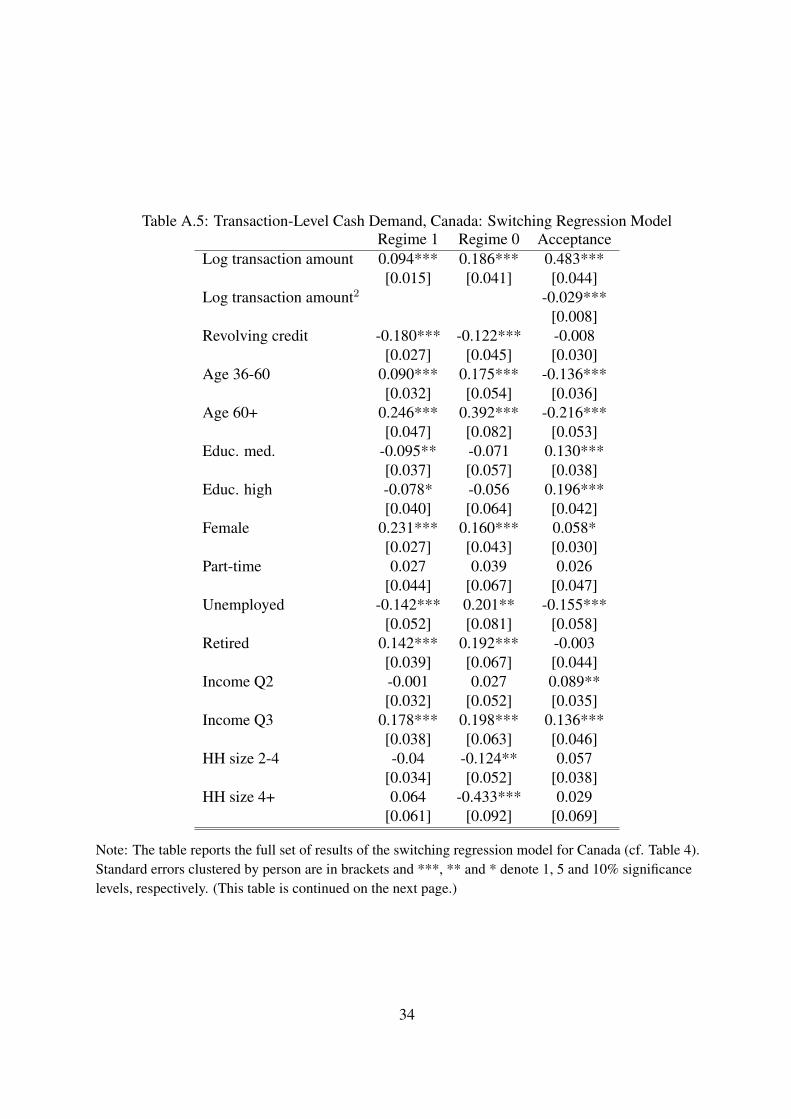
Table A.5: Transaction-Level Cash Demand, Canada: Switching Regression ModelRegime 1 Regime 0 Acceptance

Log transaction amount 0.094*** 0.186*** 0.483***[0.015] [0.041] [0.044]

Log transaction amount2 -0.029***[0.008]

Revolving credit -0.180*** -0.122*** -0.008[0.027] [0.045] [0.030]

Age 36-60 0.090*** 0.175*** -0.136***[0.032] [0.054] [0.036]

Age 60+ 0.246*** 0.392*** -0.216***[0.047] [0.082] [0.053]

Educ. med. -0.095** -0.071 0.130***[0.037] [0.057] [0.038]

Educ. high -0.078* -0.056 0.196***[0.040] [0.064] [0.042]

Female 0.231*** 0.160*** 0.058*[0.027] [0.043] [0.030]

Part-time 0.027 0.039 0.026[0.044] [0.067] [0.047]

Unemployed -0.142*** 0.201** -0.155***[0.052] [0.081] [0.058]

Retired 0.142*** 0.192*** -0.003[0.039] [0.067] [0.044]

Income Q2 -0.001 0.027 0.089**[0.032] [0.052] [0.035]

Income Q3 0.178*** 0.198*** 0.136***[0.038] [0.063] [0.046]

HH size 2-4 -0.04 -0.124** 0.057[0.034] [0.052] [0.038]

HH size 4+ 0.064 -0.433*** 0.029[0.061] [0.092] [0.069]

Note: The table reports the full set of results of the switching regression model for Canada (cf. Table 4).Standard errors clustered by person are in brackets and ***, ** and * denote 1, 5 and 10% significancelevels, respectively. (This table is continued on the next page.)

34

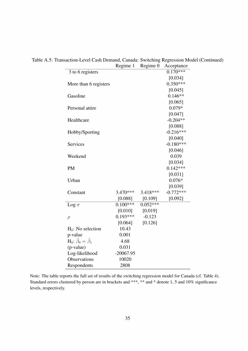
Table A.5: Transaction-Level Cash Demand, Canada: Switching Regression Model (Continued)Regime 1 Regime 0 Acceptance

3 to 6 registers 0.170***[0.034]

More than 6 registers 0.350***[0.045]

Gasoline 0.146**[0.065]

Personal attire 0.079*[0.047]

Healthcare -0.204**[0.088]

Hobby/Sporting -0.216***[0.040]

Services -0.180***[0.046]

Weekend 0.039[0.034]

PM 0.142***[0.031]

Urban 0.076*[0.039]

Constant 3.470*** 3.418*** -0.772***[0.088] [0.109] [0.092]

Log σ 0.100*** 0.052***[0.010] [0.019]

ρ 0.193*** -0.123[0.064] [0.126]

H0: No selection 10.43p-value 0.001H0: β0 = β1 4.68(p-value) 0.031Log-likelihood -20067.95Observations 10020Respondents 2808

Note: The table reports the full set of results of the switching regression model for Canada (cf. Table 4).Standard errors clustered by person are in brackets and ***, ** and * denote 1, 5 and 10% significancelevels, respectively.

35

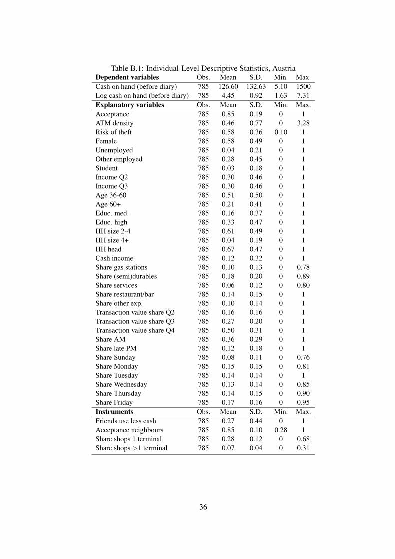
Table B.1: Individual-Level Descriptive Statistics, AustriaDependent variables Obs. Mean S.D. Min. Max.Cash on hand (before diary) 785 126.60 132.63 5.10 1500Log cash on hand (before diary) 785 4.45 0.92 1.63 7.31Explanatory variables Obs. Mean S.D. Min. Max.Acceptance 785 0.85 0.19 0 1ATM density 785 0.46 0.77 0 3.28Risk of theft 785 0.58 0.36 0.10 1Female 785 0.58 0.49 0 1Unemployed 785 0.04 0.21 0 1Other employed 785 0.28 0.45 0 1Student 785 0.03 0.18 0 1Income Q2 785 0.30 0.46 0 1Income Q3 785 0.30 0.46 0 1Age 36-60 785 0.51 0.50 0 1Age 60+ 785 0.21 0.41 0 1Educ. med. 785 0.16 0.37 0 1Educ. high 785 0.33 0.47 0 1HH size 2-4 785 0.61 0.49 0 1HH size 4+ 785 0.04 0.19 0 1HH head 785 0.67 0.47 0 1Cash income 785 0.12 0.32 0 1Share gas stations 785 0.10 0.13 0 0.78Share (semi)durables 785 0.18 0.20 0 0.89Share services 785 0.06 0.12 0 0.80Share restaurant/bar 785 0.14 0.15 0 1Share other exp. 785 0.10 0.14 0 1Transaction value share Q2 785 0.16 0.16 0 1Transaction value share Q3 785 0.27 0.20 0 1Transaction value share Q4 785 0.50 0.31 0 1Share AM 785 0.36 0.29 0 1Share late PM 785 0.12 0.18 0 1Share Sunday 785 0.08 0.11 0 0.76Share Monday 785 0.15 0.15 0 0.81Share Tuesday 785 0.14 0.14 0 1Share Wednesday 785 0.13 0.14 0 0.85Share Thursday 785 0.14 0.15 0 0.90Share Friday 785 0.17 0.16 0 0.95Instruments Obs. Mean S.D. Min. Max.Friends use less cash 785 0.27 0.44 0 1Acceptance neighbours 785 0.85 0.10 0.28 1Share shops 1 terminal 785 0.28 0.12 0 0.68Share shops >1 terminal 785 0.07 0.04 0 0.31

36

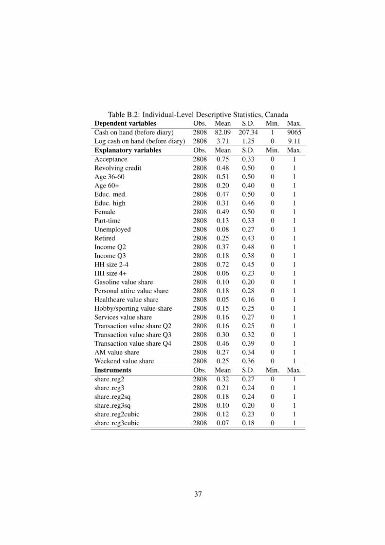
Table B.2: Individual-Level Descriptive Statistics, CanadaDependent variables Obs. Mean S.D. Min. Max.Cash on hand (before diary) 2808 82.09 207.34 1 9065Log cash on hand (before diary) 2808 3.71 1.25 0 9.11Explanatory variables Obs. Mean S.D. Min. Max.Acceptance 2808 0.75 0.33 0 1Revolving credit 2808 0.48 0.50 0 1Age 36-60 2808 0.51 0.50 0 1Age 60+ 2808 0.20 0.40 0 1Educ. med. 2808 0.47 0.50 0 1Educ. high 2808 0.31 0.46 0 1Female 2808 0.49 0.50 0 1Part-time 2808 0.13 0.33 0 1Unemployed 2808 0.08 0.27 0 1Retired 2808 0.25 0.43 0 1Income Q2 2808 0.37 0.48 0 1Income Q3 2808 0.18 0.38 0 1HH size 2-4 2808 0.72 0.45 0 1HH size 4+ 2808 0.06 0.23 0 1Gasoline value share 2808 0.10 0.20 0 1Personal attire value share 2808 0.18 0.28 0 1Healthcare value share 2808 0.05 0.16 0 1Hobby/sporting value share 2808 0.15 0.25 0 1Services value share 2808 0.16 0.27 0 1Transaction value share Q2 2808 0.16 0.25 0 1Transaction value share Q3 2808 0.30 0.32 0 1Transaction value share Q4 2808 0.46 0.39 0 1AM value share 2808 0.27 0.34 0 1Weekend value share 2808 0.25 0.36 0 1Instruments Obs. Mean S.D. Min. Max.share reg2 2808 0.32 0.27 0 1share reg3 2808 0.21 0.24 0 1share reg2sq 2808 0.18 0.24 0 1share reg3sq 2808 0.10 0.20 0 1share reg2cubic 2808 0.12 0.23 0 1share reg3cubic 2808 0.07 0.18 0 1

37

Table B.3: Transaction-Level Descriptive Statistics, AustriaDependent variables Obs. Mean S.D. Min. Max.Cash on hand 5790 128.22 146.11 0.10 1500Log cash on hand 5790 4.41 1 -2.30 7.31Acceptance 5790 0.76 0.42 0 1Explanatory variables Obs. Mean S.D. Min. Max.Log transaction amount 5790 2.62 1.16 -1.77 6.11Log transaction amount2 5790 8.23 6.18 0 37.30Gas stations 5790 0.06 0.24 0 1Semi-durables 5790 0.13 0.34 0 1Services 5790 0.05 0.22 0 1Restaurant/bar 5790 0.18 0.38 0 1Other expenses 5790 0.12 0.33 0 1AM 5790 0.37 0.48 0 1Late PM 5790 0.11 0.32 0 1Sunday 5790 0.08 0.27 0 1Tuesday 5790 0.15 0.36 0 1Wednesday 5790 0.14 0.35 0 1Thursday 5790 0.16 0.37 0 1Friday 5790 0.15 0.36 0 1Saturday 5790 0.16 0.37 0 1Typical week 5790 0.75 0.43 0 1

Table B.4: Transaction-Level Descriptive Statistics, CanadaDependent variables Obs. Mean S.D. Min. Max.Cash on hand 10020 97.14 166.66 0.02 9135Log cash on hand 10020 3.99 1.13 -3.91 9.12Acceptance 10020 0.74 0.44 0 1Explanatory variables Obs. Mean S.D. Min. Max.Log transaction amount 10020 2.81 1.28 -1.56 8.27Log transaction amount2 10020 9.51 7.55 0 68.37Gasoline 10020 0.08 0.28 0 1Personal attire 10020 0.16 0.37 0 1Healthcare 10020 0.03 0.17 0 1Hobby/sporting 10020 0.22 0.41 0 1Services 10020 0.14 0.34 0 1Weekend 10020 0.26 0.44 0 1PM 10020 0.7 0.46 0 1Urban 10020 0.83 0.38 0 1Revolving credit 10020 0.5 0.5 0 1

38

Index of Working Papers: January 30, 2009

Claudia Kwapil, Johann Scharler

149 Expected Monetary Policy and the Dynamics of Bank Lending Rates

February 5, 2009

Thomas Breuer, Martin Jandač ka, Klaus Rheinberger, Martin Summer

150 How to find plausible, severe, and useful stress scenarios

February 11, 2009

Martin Schneider, Christian Ragacs

151 Why did we fail to predict GDP during the last cycle? A breakdown of forecast errors for Austria

February 16, 2009

Burkhard Raunig, Martin Scheicher

152 Are Banks Different? Evidence from the CDS Market

March 11, 2009

Markus Knell, Alfred Stiglbauer

153 The Impact of Reference Norms on Inflation Persistence When Wages are Staggered

May 14, 2009 Tarek A. Hassan

154 Country Size, Currency Unions, and International Asset Returns

May 14, 2009 Anton Korinek

155 Systemic Risk: Amplification Effects, Externalities, and Policy Responses

May 29, 2009 Helmut Elsinger

156 Financial Networks, Cross Holdings, and Limited Liability

July 20, 2009 Simona Delle Chiaie

157 The sensitivity of DSGE models’ results to data detrending

November 10, 2009

Markus Knell Helmut Stix

158 Trust in Banks? Evidence from normal times and from times of crises

November 27, 2009

Thomas Scheiber Helmut Stix

159 Euroization in Central, Eastern and South-eastern Europe – New Evidence On Its Extent and Some Evidence On Its Causes

January 11, 2010

Jesús Crespo Cuaresma Martin Feldircher

160 Spatial Filtering, Model Uncertainty and the Speed of Income Convergence in Europe

March 29, 2010

Markus Knell

161 Nominal and Real Wage Rigidities. In Theory and in Europe

May 31, 2010 Zeno Enders Philip Jung Gernot J. Müller

162 Has the Euro changed the Business Cycle?

August 25, 2010

Marianna Č ervená Martin Schneider

163 Short-term forecasting GDP with a DSGE model augmented by monthly indicators

September 8, 2010

Sylvia Kaufmann Johann Scharler

164 Bank-Lending Standards, the Cost Channel and Inflation Dynamics

September 15, 2010

Helmut Elsinger

165 Independence Tests based on Symbolic Dynamics

December 14, 2010

Claudia Kwapil

166 Firms' Reactions to the Crisis and their Consequences for the Labour Market. Results of a Company Survey conducted in Austria

May 10, 2011 Helmut Stix

167 Does the Broad Public Want to Consolidate Public Debt? – The Role of Fairness and of Policy Credibility

May 11, 2011 Burkhard Raunig, Johann Scharler

168 Stock Market Volatility, Consumption and Investment; An Evaluation of the Uncertainty Hypothesis Using Post-War U.S. Data

May 23, 2011 Steffen Osterloh 169 Can Regional Transfers Buy Public Support? Evidence from EU Structural Policy

May 23, 2011 Friederike Niepmann Tim Schmidt-Eisenlohr

170 Bank Bailouts, International Linkages and Cooperation

September 1, 2011

Jarko Fidrmuc, Mariya Hake, Helmut Stix

171 Households’ Foreign Currency Borrowing in Central and Eastern Europe

September 9, 2011

Jürgen Eichberger, Klaus Rheinberger, Martin Summer

172 Credit Risk in General Equilibrium

October 6, 2011

Peter Lindner 173 Decomposition of Wealth and Income using Micro Data from Austria

October 18, 2011

Stefan Kerbl 174 Regulatory Medicine Against Financial Market Instability: What Helps And What Hurts?

December 31, 2011

Konstantins Benkovskis Julia Wörz

175 How Does Quality Impact on Import Prices?

January 17, 2012

Nicolás Albacete 176 Multiple Imputation in the Austrian Household Survey on Housing Wealth

January 27, 2012

Gerhard Fenz, Lukas Reiss, Martin Schneider

177 A structural interpretation of the impact of the great recession on the Austrian economy using an estimated DSGE model

July 27, 2012

Helmut Stix

178 Why Do People Save in Cash? Distrust, Memories of Banking Crises, Weak Institutions and Dollarization

August 20, 2012

Markus Knell

179 Increasing Life Expectancy and Pay-As-You-Go Pension Systems

September 25, 2012

Fabio Rumler, Walter Waschiczek

180 Have Changes in the Financial Structure Affected Bank Protability? Evidence for Austria

November 9, 2012

Elisabeth Beckmann, Jarko Fidrmuc, Helmut Stix

181 Foreign Currency Loans and Loan Arrears of Households in Central and Eastern Europe

June 10, 2013

Luca Fornaro

182 International Debt Deleveraging

June 10, 2013

Jenny Simon, Justin Valasek

183 Efficient Fiscal Spending by Supranational Unions

July 24, 2013

Thomas Breuer, Hans-Joachim Vollbrecht, Martin Summer

184 Endogenous Leverage and Asset Pricing in Double Auctions

September 23, 2013

Martin Feldkircher 185 A Global Macro Model for Emerging Europe

September 25, 2013

Martin Gächter, Aleksandra Riedl

186 One Money, One Cycle? The EMU Experience

December 9, 2013

Stefan Niemann, Paul Pichler

187 Collateral, Liquidity and Debt Sustainability

March 6, 2014

Elisabeth Beckmann, Helmut Stix

188 Foreign currency borrowing and knowledge about exchange rate risk

March 10, 2014

Jesús Crespo Cuaresma, Martin Feldkircher, Florian Huber

189 Forecasting with Bayesian Global Vector Autoregressive Models: A Comparison of Priors

May 12, 2014

Claudia Steinwender 190 Information Frictions and the Law of One Price: “When the States and the Kingdom became United”

May 12, 2014

Saleem A. Bahaj 191 Systemic Sovereign Risk: Macroeconomic Implications in the Euro Area

May 16, 2014

John Bagnall, David Bounie, Kim P. Huynh, Anneke Kosse, Tobias Schmidt, Scott Schuh and Helmut Stix

192 Consumer Cash Usage: A Cross-Country Comparison with Payment Diary Survey Data

May 19, 2014

Konstantins Benkovskis Julia Wörz

193 “Made in China” - How Does it Affect Measures of Competitiveness?

June 25, 2014

Burkhard Raunig, Johann Scharler and Friedrich Sindermann

194 Do Banks Lend Less in Uncertain Times?

July 28, 2014

Martin Feldkircher and Florian Huber

195 The International Transmission of U.S. Structural Shocks – Evidence from Global Vector Autoregressions

September 16, 2014

Kim P. Huynh, Philipp Schmidt-Dengler, Helmut Stix

196 The Role of Card Acceptance in the Transaction; Demand for Money

Call for Applications: Visiting Research Program

The Oesterreichische Nationalbank (OeNB) invites applications from external researchers for participation in a Visiting Research Program established by the OeNB’s Economic Analysis and Research Department. The purpose of this program is to enhance cooperation with members of academic and research institutions (preferably post-doc) who work in the fields of macroeconomics, international economics or financial economics and/or with a regional focus on Central, Eastern and Southeastern Europe.

The OeNB offers a stimulating and professional research environment in close proximity to the policymaking process. Visiting researchers are expected to collaborate with the OeNB’s research staff on a prespecified topic and to participate actively in the department’s internal seminars and other research activities. They will be provided with accommodation on demand and will, as a rule, have access to the department’s computer resources. Their research output may be published in one of the department’s publication outlets or as an OeNB Working Paper. Research visits should ideally last between 3 and 6 months, but timing is flexible.

Applications (in English) should include

− a curriculum vitae,

− a research proposal that motivates and clearly describes the envisaged research project,

− an indication of the period envisaged for the research visit, and

− information on previous scientific work.

Applications for 2014 should be e-mailed to eva.gehringer-wasserbauer@oenb.at by November 1, 2014.

Applicants will be notified of the jury’s decision by mid-December. The following round of applications will close on May 1, 2015.