WORKING PAPER

1750 Massachusetts Avenue, NW | Washington, DC 20036-1903 USA | 202.328.9000 Tel | 202.328.5432 Fax | www.piie.com

18-1 ECB Interventions in Distressed Sovereign Debt Markets: The Case of Greek BondsChristoph Trebesch and Jeromin ZettelmeyerJanuary 2018

Abstract

We study central bank interventions in times of severe distress (mid-2010), using a unique bond-level dataset of ECB purchases of Greek sovereign debt. ECB bond buying had a large impact on the price of short and medium maturity bonds, resulting in a remarkable “twist” of the Greek yield curve. However, the effects were limited to those sovereign bonds actually bought. We find little evidence for positive effects on market quality, or spillovers to close substitute bonds, CDS markets, or corporate bonds. Hence, our findings attest to the power of central bank intervention in times of crisis but also suggest that in highly distressed situations, this power may not extend beyond those assets actually purchased.

JEL Codes: E430, E580, F340, G120.Keywords: Central Bank Asset Purchases, Securities Markets Programme,

Eurozone Crisis, Sovereign Risk, Market Segmentation

Christoph Trebesch is professor and head of research area “Global Macroeconomics” at Kiel Institute for the World Economy and Department of Economics, Kiel University. Jeromin Zettelmeyer is senior fellow at the Peterson Institute for International Economics.

Authors’ Note: This paper is forthcoming in the IMF Economic Review. We are grateful to Bennet Berger, Alvaro Leandro, Adrian Rott and Maximilian Rupps for excellent research assistance, Christine Sheeka for helpful informa-tion on the MTS high frequency data, Jonathan Lehne, Olga Ponomarenko, and Kristjan Piilmann for assisting us with the collection of Bloomberg data and Egor Gornostay for his careful fact checking. We also thank the editor, several anonymous referees, Henrique Basso, Benjamin Böninghausen, Giovanni Dell’Ariccia, Marcel Fratzscher, Thomas King, Sergi Lanau, Athanasios Orphanides, Seth Pruitt, Julian Schumacher, Bernd Schwaab Andrei Shleifer, Linda Tesar, Julian Williams, and seminar participants at the ECB, the Federal Reserve Bank of Chicago, the Federal Reserve Bank of San Francisco, the Bank of Spain, the LSE Financial Markets Group, ZEW Mannheim, and the Universities of Frankfurt (Goethe), Mainz, Munich, and Santa Clara for helpful comments and suggestions. Part of this paper was written while Trebesch was visiting the IMF. An early version of this paper was circulated under the title: “Deciphering the ECB Securities Market Programme: The Case of Greek Bonds.” The views expressed in this paper are those of the authors and not those of the institutions they are affiliated with.

© Peterson Institute for International Economics. All rights reserved. This publication has been subjected to a prepublication peer review intended to ensure analytical quality.

The views expressed are those of the authors. This publication is part of the overall program of the Peterson Institute for International Economics, as endorsed by its Board of Directors, but it does not neces-

sarily reflect the views of individual members of the Board or of the Institute’s staff or management. The Peterson Institute for International Economics is a private nonpartisan, nonprofit institution for rigorous,

intellectually open, and indepth study and discussion of international economic policy. Its purpose is to identify and analyze important issues to make globalization beneficial and sustainable for the people of the United States and the world, and then to develop and communicate practical new approaches for dealing with them. Its work is funded by a highly diverse group of philanthropic foundations, private

corporations, and interested individuals, as well as income on its capital fund. About 35 percent of the Institute’s resources in its latest fiscal year were provided by contributors from outside the United States.

A list of all financial supporters is posted at https://piie.com/sites/default/files/supporters.pdf.

1

1. Introduction

The ECB’s “Securities Markets Programme” (SMP) was one of the most controversial

sovereign bond buying operations ever implemented by a central bank. It was also the

precursor to the “Outright Monetary Transactions” (OMT) programme, which has been central

to the ECB’s strategy to resolve the Eurozone crisis since September 2012. Despite this,

relatively little is known about the determinants and effects of the SMP, in part because the

ECB did not reveal which bonds it bought, in what amounts, and when.1 As a result,

researchers cannot easily assess the SMP and its effects, even though the large-scale purchases

during the height of the Eurozone crisis should provide an excellent testing ground for theories

of bond supply and limits to arbitrage.2 This paper helps to fill this gap, by conducting the first

bond-level analysis (to our knowledge) of ECB purchases in the Eurozone debt crisis.

To measure bond-level purchases we make use of the fact that the ECB did not participate in

the Greek sovereign debt restructuring of 2012, thereby revealing its stock of holdings.

Specifically, we obtained a little-known, Greek-language government gazette, which lists the

ECB’s holdings across all 81 Greek sovereign bonds outstanding in February 2012, just prior

to the Greek bond exchange.3 These data allow us to shed light on how the ECB intervened in

distressed sovereign bond markets, in particular which Greek instruments it bought. Total ECB

holdings were €42.7bn, more than 15% of the total Greek bond market, with a large variation

in the amounts of bonds purchased. The ECB only bought a subset of 31 out of the 81 Greek

bonds outstanding and it favoured large benchmark bonds with a maturity of less than 10 years,

and with comparatively high yields.

The main objective of the paper is to study the effects of the ECB interventions on bond yields,

bond liquidity and bond price volatility. To do this, we exploit the cross-sectional variation in

bond purchases and compare changes in yields, liquidity and volatility of targeted and non-

targeted bonds. This allows us to isolate the effect of purchases from news and other factors

that might have influenced bond yields during the intervention period. We focus on the first

phase of the SMP, May and June 2010, when more than 10% of the total stock of Greek bonds

1 The ECB only published weekly aggregate purchase amounts as well as a one-time snapshot of the country composition of the bond portfolio acquired through the SMP. See http://www.ecb.int/press/pr/date/2013/html/pr130221_1.en.html. 2 The ECB purchases were large and very concentrated and they took place at a time of high uncertainty and risk aversion. In such an environment limits to arbitrage should matter most (Vayanos and Vila 2009). 3 We are grateful to Sergi Lanau for pointing us to this source. Technically, the gazette shows the results of the “silent” ECB debt swap. On February 17, 2012, all bonds held by the ECB and other central banks were exchanged into new bonds which were exactly the same as the old ones (same nominal amount, coupon payments, and repayment dates) but which were given a new set of serial numbers (ISINs).

2

was taken out of the market by the ECB, resulting in a sudden shift in bond supply.4 To deal

with endogeneity and selection effects – in particular the possibility that the ECB targeted

under-priced bonds – we control for pre-SMP yields and run two-stage least squares

regressions, using bond characteristics that are correlated with ECB intervention (but should

not affect bond prices) as instruments. For robustness, we also use a difference-in-difference

estimation approach, which helps account for unobserved bond characteristics. We attempt to

control for changes in bond-specific default risk (proxied by changes in CDS prices at various

maturities), differences in legal risk (proxied by governing law), and potential term structure

effects.

Our main finding is that the effect of interventions on bond yields was large but “local”.

According to our estimation results, €1bn of ECB purchases, which corresponds to 16.6% of

the outstanding face value of bonds purchased by the ECB on average, translates into a yield

drop between 80 to 190 basis points in that series during the 8 weeks following the start of the

SMP on May 10, 2010. The exact point estimate depends on the sample, estimation method

and data used. Based on these findings, a back-of-the envelope calculation suggests that the

total decline in Greek yields attributable to ECB purchases was in the same order of magnitude.

The effects were particularly pronounced at the short end of the yield curve (up to 7 years

maturity), where the ECB intervened the most. The Greek yield curve turned from downward

sloping to well-behaved in a matter of days, at a speed and scale rarely seen in an advanced

economy. This remarkable “twist” of the yield curve is closely related to the volume of ECB

interventions in each maturity segment. Hence, interventions in Greece were most effective

for short-maturity bonds. This is consistent with the design of the OMT and Aguiar and

Amador (2013) who suggest to “take the short route” to calm sovereign distress.5

In principle, there could be several explanations as to why ECB intervention had these large

bond-specific effects. First, an “expected loss channel”: ECB purchases of certain bonds could

have made these assets safer, in the eyes of investors, with lower default risk and/or lower

expected loss-given-default compared to bonds that were not purchased. Second, a “liquidity

channel”: as a large buyer in a distressed market, the ECB could have lowered the search costs

of finding a buyer, hence reducing liquidity premiums of individual bonds or bond segments

(see Duffie et al. 2005, 2007 and De Pooter et al. 2016). Finally, a channel that is variously

referred to as a “scarcity”, “portfolio balance”, “preferred habitat”, or “local supply” effect.

4 In this period, the amount of outstanding debt was essentially fixed since the Greek government was excluded from capital markets from April 2010 onwards, making the bond supply shocks caused by the ECB even more pronounced. See section 2 and Appendix A for a discussion on the timing of purchases. 5 The OMT programme would focus, in particular, “on sovereign bonds with a maturity of between one and three years.” http://www.ecb.int/press/pr/date/2012/html/pr120906_1.en.html.

3

Vayanos and Vila (2009) and Greenwood and Vayanos (2014) suggest that investors can have

a preference for particular bonds, e.g. because they are interested in a specific maturity. A

change in bond supply could then result in a change in bond prices if financial frictions – such

as risk aversion in a crisis period – introduce limits to arbitrage across similar assets. In that

case, central bank bond purchases would affect the yields of individual bonds or bond

segments, as shown by D’Amico and King (2013) for the United States.6

Our data allow us to test for the first two channels directly, using maturity-specific CDS-

spreads – that should pick up default risk effects of intervention in particular segments of the

yield curve – and measures of bond liquidity, such as bid-ask spreads and bond quote

frequency. We find little if any evidence that intervention influenced either maturity-specific

default risk or bond-level liquidity. Hence,we conclude that “local supply” effects must have

been the main channel through which intervention affected bond yields.

While ECB purchases had a large impact on bonds actually bought, they seem to have affected

only those bonds. The effects of intervention on Greek bonds seem to have been much more

localized than in the US or the UK context. We find no evidence for spill-over effects of

purchases on close substitute sovereign bonds (those with similar maturity), suggesting highly

segmented markets. There is also only limited evidence for an improvement of CDS market

quality or for spill-overs to the corporate bond market. While we show that the CDS-bond

basis and bond price volatility decreased post-intervention, this is again mostly for the bonds

targeted and less so for the remainder of the market.

Consistent with the aforementioned theories of bond supply, we interpret the highly localized

effects as the result of risk-aversion and limits to arbitrage. The central bank bond purchases

in Greece occurred in the middle of a debt crisis, in which markets where comparatively

illiquid, and arbitrage across close substitute bonds was much more costly than it was in the

US or the UK. By mid-2010, Greek sovereign bonds had turned into a volatile and

“information sensitive” asset, introducing informational frictions (Brunnermeier et al. 2012)

and making the bonds less attractive to outsiders such as foreign institutional investors. At the

same time, Greek banks, the natural domestic traders of Greek sovereign bonds, were coming

under pressure due to high sovereign exposures, limiting their ability to render the yield-curve

arbitrage-free.7

6 See also Gürkaynak and Wright (2012), for a survey. 7 Acharya et al. (2014) show how a sovereign-bank doom loop can limit the trading and investment abilities of domestic banks.

4

The paper forms part of a growing literature on the effects of central bank asset purchases,

which so far has mostly focused on the Large Scale Asset Purchase Programmes (LSAP) by

the Federal Reserve Bank and the quantitative easing (QE) programmes by the Bank of

England.8 Our approach is closest to D’Amico and King (2013) for the US and Joyce and Tong

(2012) for the UK, who both exploit bond-level data to identify the effect of bond purchases.

Compared to these papers, we find larger and more localized effects of purchases in the Greek

crisis, when levels of risk aversion are likely to have been particularly high.9

Regarding the impact of ECB interventions in sovereign bond markets, we are aware of five

principal contributions written in parallel with the present paper, namely De Pooter et al.

(2015), Doran et al. (2014), Eser and Schwaab (2016), Ghysels et al. (2017) and

Krishnamurthy et al. (2015).10 De Pooter et al. (2015) use weekly estimates of the amount of

SMP purchases from Barclays and focus on the effect on liquidity premiums of 5-year bonds,

proxied by the difference between implied default probabilities in CDS and bond spreads,

while Krishnamurthy et al. (2014) assess the impact of the SMP and OMT announcements on

sovereign and corporate bond markets of the Eurozone. The remaining three papers examine

the impact of SMP purchases on the bond markets in which the SMP was active, using

confidential ECB data which identifies the purchase date. Apart from the data, the main

difference between these papers and ours consists in the identification strategy. Doran et al.

(2014) and Ghysels et al. (2017) show that ECB purchases on given dates were to some extent

responses to within-day yield changes, as one would expect if the ECB followed an

intervention strategy that attempted to stabilise yields.11 To disentangle cause and effect of

purchases and yields, they use very high frequency intraday data. Eser and Schwaab (2016)

run a panel regression using daily changes in the yields 5-year benchmark bonds as dependent

variable, and total daily purchase amounts by country. This identifies the effect of the SMP

using a combination of daily time series variation and cross-country variation, which is a valid

approach so long as any bias resulting from within-day endogeneity of ECB purchases is small.

8 The impact of the Federal Reserve’s LSAP is analysed in Gagnon et al. (2011), Krishnamurthy and Vissing-Jorgensen (2011), Bauer and Rudebusch (2013), D’Amico et al. (2012), Hamilton and Wu (2012), Cahill et al. (2013) and D'Amico and King (2013). For evidence on the UK’s QE, see Joyce et al. (2011) and Joyce and Tong (2012). More general papers on the relation of bond prices and bond supply include Bernanke et al. (2004), Greenwood and Vayanos (2010, 2014), and Krishnamurthy and Vissing-Jorgensen (2012). 9 Our estimated total programme effect in mid-2010 (-185 to -75 basis points) compares to a total impact of about -30 to -50 basis points for the first LSAP programme of the Federal Reserve, according to D’Amico and King (2013), and approximately matches the announcement effect of QE in the UK, according to Joyce and Tong (2012). Interestingly, the latter find no bond-specific effects of purchases on yields (no “own purchase” effect like us). See the survey by the IMF (2013) for a comparison of the impact of bond purchase programmes. 10 In addition, Beetsma et al (2014) examine the effect of aggregate weekly SMP purchases in a study of the effect of news on the intraday volatility and covariance of Euro area bond yields and find a mitigating effect. 11 Our intraday results for May 10, 2010, are consistent with Doran et al. (2013), since we also find purchases to have halted price declines over the trading day, but only for targeted bonds.

5

In contrast, our paper identifies the effects of the SMP using the cross-sectional variation in

purchases between targeted and non-targeted bonds within one country. This helps to

disentangle purchase effects from country-level confounding factors such as news shocks. It

also enables us to side-step the key endogeneity problem bedevilling the time series approach,

namely, that the ECB chose the moment and extent of its interventions so as to lean against

pressures on bond markets. This said, an analogous endogeneity problem could arise in our

data if the ECB selected bonds for intervention based on characteristics that might have

influenced the subsequent evolution of yields directly. We check whether this brand of

endogeneity might have been present, and find that the ECB did in fact target bonds whose

yields had been rising particularly sharply in the weeks prior to the launch of the SMP. If the

yields of these bonds displayed a tendency to revert more quickly to normal levels after the

SMP announcement than yields that rose less sharply, this would upward-bias the estimated

purchase effects. We use several approaches to deal with this potential bias, including

controlling for pre-crisis yields movements in several ways, and two-stage least squares

estimation using bond characteristics as instruments that are correlated with selection but

should not predict changes in yields, with consistent results.

One of our main findings is that there were stark differences in the impact of the programme

across types of bonds and maturities, because interventions targeted specific bonds, and had

largely “local” effects. Methodologically, our results can therefore also be read as a warning

against using benchmark bonds without accounting for how much these bonds were actually

purchased: in a segmented bond market, the yield of a single 5-year or 10-year bond may not

provide a representative estimate of effect of intervention. Neither would artificial benchmark

yields or bond indices that aggregate price/yield quotes from different bonds, since these may

represent a mix of bonds that were bought and bonds that were not bought. This may help

explain why we find strong and significant effects of the SMP in the case of Greece, while

time series studies using indices or artificial benchmarks do not.12

The section that follows describes the SMP and the data used, and characterizes ECB

purchasing patterns in the case of Greece. In sections 3 and 4 we turn to the effects of

intervention using graphical and regression analysis. Importantly, subsection 3.5 discusses the

potential channels behind our main findings, while section 5 focuses on market quality effects.

12 Conversely, it may also help explain why we do not find a liquidity impact of ECB purchases although – consistent with the findings of De Pooter et al (2016) and Eser and Schwab – bid-ask spreads declined on average during the intervention period. This decline appears to have reflected SMP and EFSF announcements, which lowered perceived default risk, rather than bond-level intervention.

6

2. Institutional context and data

2.1 The ECB Securities Markets Programme

The SMP was announced on Sunday, May 9, 2010, and launched one day later. The (largely

unexpected) inception of the programme followed an escalation of the Eurozone debt crisis in

April, with widening yield spreads across the Eurozone periphery. Greece posed the most

urgent problem, since it had large bond amortisations due in mid-May, and seemed on the

verge of losing market access.13 On May 2, following weeks of frantic negotiations, EU

Commissioner Olli Rehn and IMF Managing Director Dominique Strauss-Kahn released a

joint statement announcing a €110 billion rescue programme for Greece. This was followed

by the announcement of the SMP, the fast-track approval of the Greek rescue programme by

the IMF board, and the creation of the EFSF, a €440 billion crisis facility for Eurozone

countries, late on May 9. On May 10, the first trading day after the announcement, the ECB

released a statement describing the programme, with further details published on May 14.14

There were two main phases of SMP activism. We focus on the first 8 weeks of interventions,

which lasted from the inception of the programme, on May 10, until early July of 2010. Bond

purchases in this phase focused on Greek, Irish, and Portuguese debt.15 After 12 months with

little or no purchases, the ECB announced a reactivation of the SMP on August 7, 2011, giving

rise to the second phase of bond purchases, which lasted until December 2011 and focused on

Spanish and Italian bonds.16 Interventions were larger than before and the ECB tripled its stock

of holdings from €70bn to over €200bn (at market prices). The programme officially ended in

September 2012 with the introduction of a successor programme, the OMT, which so far has

not been activated. Figure A1 in the Appendix shows the aggregate weekly SMP purchases

from May 2010 until July 2012.

There are several important differences between the ECB’s SMP and the bond purchase

programmes in the US and the UK. Unlike the US and UK programmes, which began a year

earlier,17 the SMP’s objective was not to ease monetary conditions but rather to contain the

debt crisis in specific Eurozone countries. The official argument was that the SMP would help

restore normal transmission of monetary policy in crisis countries by ensuring “depth and

13 For a contemporaneous account see, Nelson et al (2010) 14 See http://www.ecb.int/ecb/legal/pdf/l_12420100520en00080009.pdf. 15 See Doran et al. (2013), Eser and Schwab (2015) and for a contemporary view, Hume (2010). 16 See “Statement by the President of the ECB” from 7 August 2011: http://www.ecb.europa.eu/press/pr/date/2011/html/pr110807.en.html. Ghysels et al. (2014), Wall Street Journal, 8/8/2011 “ECB Buys Italian, Spanish Bonds”, and Zerohedge, http://www.zerohedge.com/news/ecb-purchases-%E2%82%AC22-billion-italian-spanish-bonds-past-week-highest-weekly-amount-ever. 17 See IMF (2013) for an overview.

7

liquidity in those market segments which are dysfunctional.”18 ECB board members repeatedly

emphasised that all bond purchases would be sterilised. Another difference is that the ECB

committed to a policy of holding the bonds it bought until maturity, unlike the central banks

of the UK or the US.19 Figure A1 shows that the size of the SMP portfolio grew in line with

the weekly purchase amounts. Minor decreases in the total stock of holdings that are visible

around some dates were due to maturing securities, not bond sales.

Most critically, from the perspective of identifying its effects, SMP purchases were not made

transparent. Unlike the US and UK programmes, the ECB set no time frame and no target

levels in its interventions, and did not reveal which bonds it purchased and when and in what

amounts they were purchased (even at the country level). Purchases took place in the non-

anonymous dealer market, with offers being made to several (typically, 3-5) dealers

simultaneously on a request-for-quote basis. The only way market participants could learn

what was being bought was hence to participate in an actual transaction (i.e., be chosen as a

potential buyer by the ECB), or to hear from other dealers that participated. This said, the

market is likely to have quickly formed expectations on types of bonds that were being bought,

based both on actual purchases and on the ECB collateral policy (the ECB only bought Greek

bonds that were eligible as collateral).

2.2 ECB purchase data at the bond-level

A distinguishing feature of this paper is that we analyse ECB bond purchases at the level of

individual bonds, and not in the aggregate. To identify the bonds bought by the ECB we take

advantage of the historic Greek sovereign debt restructuring implemented between February

and April of 2012. The operation restructured all outstanding Greek government bonds owed

to private creditors, namely 81 Hellenic Republic titles with an eligible volume of €195.7bn

(see Zettelmeyer et al. 2013 for a detailed description).20

18 See http://www.ecb.int/press/pr/date/2010/html/pr100510.en.html. 19 In a related Q&A in February 2012, ECB president Draghi reconfirmed this as follows: “Question: Will you hold the bonds in your SMP programme until maturity? Draghi: We have no reason to change this commitment. If we do, we will tell you.” http://www.ecb.int/press/pressconf/2012/html/is120209.en.html. 20 In addition, the exchange involved 36 instruments issued by three public entities: Hellenic Railways, Hellenic Defence Systems, and Athens Urban Transport Organisation (“guaranteed titles”), with a volume of €9.8bn. In this paper, we ignore these quasi-sovereign bonds because none appears to have ever been purchased under the SMP, presumably because they were far less liquid, and perhaps also because their legal properties would have complicated pricing comparisons with sovereign bonds (Buchheit and Gulati, 2013). Although eligible under the SMP policy, they may not have been considered for intervention in practice and are hence suspect as controls. In any case, with few exceptions, no yield information is available for these bonds during our sample period.

8

For the purposes of our analysis, the essential feature of the Greek debt exchange is that the

ECB did not participate in it. Just before the exchange, Greek bonds held by the ECB and by

other Eurosystem central banks were exchanged into new bonds which were almost exactly

the same as the old ones (same nominal amount, coupon payments, and repayment dates)

except the fact that they were assigned new bond identifiers (ISINs) and were thereby not

eligible in the subsequent Greek debt restructuring (which targeted only the “old” ISINs).21

With this “silent swap” operation the ECB avoided taking a haircut and made its bonds

disappear from the stock of tradable Greek debt. A little-known Greek-language government

gazette lists the amount of each bond swapped by the ECB, the Eurozone national central

banks (NCBs), and the European Investment Bank (EIB), respectively, and hence reveals their

holding portfolios as of February 2012.22 For the ECB, the list contains 31 bonds with total

face value of €42.7bn, or 17% of the total stock of Greek sovereign bonds outstanding.23

Because the ECB had a buy-and-hold portfolio, this stock of holdings reflects the cumulative

amount purchased via the SMP between May 2010 and February 2012, minus purchases of

bonds that matured between May 2010 and February 2012. The NCBs held another €13.5bn

(7% of total), while the EIB held €315m.

The main limitation of this data is that they are available for only one point in time (February

2012). We do not know the purchase dates and we have no information on SMP purchases, if

any, of bonds maturing prior to February 2012.24 Despite this, we can make reasonable

assumptions on the main purchase periods based on total ECB purchase data and additional

information from market dealers and the financial press. All available evidence suggests that

the large majority of Greek bonds were purchased in the first few weeks of the SMP. Figure

A2 shows detailed weekly estimates from Barclays (2012), a major dealer in Greek bonds,

whose estimates are also used in the regressions by De Pooter et al. (2015). For our main period

of analysis, from May 10 to July 5, Barclays estimates a total amount of Greek bond purchases

of €35bn at market prices, or roughly €40bn at face value. This implies that more than 75% of

total SMP purchases of Greek bonds occurred in the first 8 weeks (after May 10). Hence, the

ECB holdings of February 2012 are a useful, albeit noisy proxy for Greek SMP bond purchases

in May and June 2010. The section on estimation strategy below discusses how we deal with

21 In addition, five foreign law bonds (including four bonds of which the ECB had bought small amounts) were swapped into Greek law bonds. In one case, held by one of the other Eurosystem central banks, the currency of denomination was swapped from US dollars to Euros. 22 Specifically, we draw on the government gazette issues “413 V/2012”, “574 V/2012”, and “705 V/2012”, published in February 2012 (in print only). We are grateful to Sergi Lanau for pointing us to this source. 23 30 of these 31 bonds were among the 81 bonds that were subsequently restructured. The remaining bond was a floating rate note that was swapped by the ECB but escaped the debt restructuring. 24 Specifically, we lack information on bonds maturing between May 2010 and February 2012 (less than 10% of total Greek bonds outstanding). Bonds at the very short-end of the yield curve are therefore excluded from our analysis, including four bonds that were trading on secondary markets in 2010 (see Appendix A).

9

the measurement error that is introduced by this proxy, while Appendix A provides a more

detailed discussion on the purchase data and its limitations.

2.3 Bond price data and control variables

Our main source of data on bond yields and bond liquidity – proxied by bid-ask spreads – is

Bloomberg, because to the best of our knowledge it provides the most reliable pricing data,

combining information from more than a dozen dealers, and also covers a wider set of Greek

sovereign bonds than other data sources – namely, 40 Greek government bonds outstanding in

February 2012, including 25 out of the 31 bond series purchased by the ECB.25

As a secondary source on bond price data, we also use the Thomson Reuters Tick History

database.26 Unlike Bloomberg, this data is available at tick frequency and provides executable

dealer price and yield quotes from the over-the-counter market.27 Although its coverage is

narrower than Bloomberg (only 31 bonds), there are three reasons to use this dataset in addition

to the Bloomberg data. First, the frequency at which specific bond series are quoted and priced

provides an additional, natural measure of liquidity, which complements bid-ask spreads.28

Second, it enables us to use intra-day information for a particular day (May 10, 2010, the day

on which the ECB began its purchases) which can give us a sense of the announcement effects

of the SMP on Greek bond yields. Third, we can use the sample of OTC-traded bonds for

robustness purposes. Overall, we find the results to be similar irrespective of the data source

used. The yield and bond price series of both datasets are very highly correlated and all of our

main graphs look alike.

Furthermore, we use Euro-denominated Greek CDS premiums from Markit as a pure measure

of Greek default and loss-given-default (LGD) risk at various maturities. CDS premiums are

well-suited to this purpose, because they are priced off relatively liquid instruments (the data

quality on Greek CDS is very high, see section 5) and because we know that the ECB did not

intervene in the CDS market. In sections 4 and 5, we use this data both as a regression control

and to examine whether ECB intervention affected bond yields by influencing default risk.

Finally, we draw on the dataset collected by Zettelmeyer et al. (2013), which is itself based on

25 Specifically, we use Bloomberg’s CBBT pricing source whenever available and the BGN source otherwise. 26 Alternative data sources that we accessed and compared include J.P. Morgan and data from the trading platform MTS. Both sources had only very restricted coverage of Greek sovereign bond prices in 2010. 27 Similar to Calice et al (2013) we compute mid-yields and mid-prices as an average of bid and ask quotes from generic identifiers (TICs) on each bond since these are the most liquid source and combines information from multiple dealers. The alternative would be to use dealer-specific quotes, but that would imply an arbitrary choice on which dealer data to use. 28 Thomson Reuters only provides data on “quote depth” (amounts offered/traded) for very few bonds.

10

the Greek debt exchange memoranda and Bloomberg data, for additional information on main

bond characteristics, such as issuance date, maturity, coupon size, or governing laws. Table

B1 in the Appendix provides a description and summary statistics for each control variable.

2.4 Characterising ECB purchases of Greek bonds

We now take a first look at the data, with the aim of characterising which types of bonds tended

to be bought by the ECB. Apart from providing some new stylised facts on ECB intervention

in crisis times, this will help us pinpoint potential endogeneity issues that may arise when we

try to assess the impact of ECB intervention on bond yields later on.

We focus on the cross-section of all Greek government bonds that were outstanding just prior

to the Greek debt exchange, and compute the share of each bond held by the ECB as a

percentage of the total amount outstanding (both in February 2012). Table A1 in the Appendix

shows that the ECB bought substantial amounts of some bond series (up to 38% of total

outstanding) but did not purchase a single bond in 51 out of the 81 Greek bond series

outstanding just before the exchange. The mean share of ECB holdings was 6.8%, with a

median of 0% and a standard deviation of 11.5 percentage points.

What accounts for this variation? Table 1 gives a descriptive overview, comparing the SMP

portfolio of Greek bonds with the full sample of 81 Greek bonds, both weighted by bond size.

The table shows that the ECB almost only bought Greek law bonds (26 out of the 31 bonds

bought, making up 99.9% of holdings compared to 92.6% in the full sample),29 despite the fact

that 28 out of the 81 instruments were issued under foreign (mostly English) law. Intervention

focused on large bonds that were traded on secondary markets and for which pricing

information was available through platforms such as Bloomberg. 95% of ECB holdings

consisted of “benchmark bonds” that were used at least once since 2000 by Bloomberg in

computing the Greek yield curve, while 80% of ECB holdings were concentrated in the 20

largest bonds. Furthermore, the ECB focused on bonds with shorter and medium maturities.

The average maturity of the Greek ECB portfolio was just 5.4 years, compared to more than 9

years in the full sample of Greek bonds (Euro-weighted and measured as of May 2010). Figure

1 confirms that the ECB had a preference for shorter-dated instruments and did not buy long-

dated bonds of more than 20 years maturity.

Finally, it appears that the ECB had a preference for bonds with higher pre-intervention yields.

To show this, we construct 4-week average yields for the pre-SMP period (i.e. from April 12

29 The exception was one English law bond maturing in 2014, of which the ECB held a small amount.

11

until May 7), using those bonds with pricing data (from Bloomberg). Table 1 shows that the

average pre-SMP yield of bonds bought by the ECB was 9.4%, compared to 8.7% in the full

sample. Figure 2 shows a striking correlation between ECB holdings (in % of total face value)

and pre-SMP bond yields. The figure looks similar when using yield spreads above German

Bunds, when using deviations of yields from a fitted yield curve, when using the increase in

yield spreads between April 12 and May 7 instead of yield levels, or when using the Euro

amount purchased instead of the share.

To further explore the characteristics of purchased bonds we run a few simple regressions with

the share of ECB purchases as dependent variable (Table 2). We start with the full sample of

81 bonds and focus on time-fixed bond characteristics, such as the outstanding amount,

coupon, maturity, and governing law. It is remarkable that just one variable - the dummy

capturing benchmark bonds or, alternatively, the variable “bond size” – can explain almost

half of the variation in bond buying patterns. Column 6 shows that in an OLS regression with

bootstrapped standard errors (to account for the small sample size), benchmark bonds are

associated with a 7.8 percentage point higher share of ECB holdings, which is larger than the

mean share of ECB holdings (6.8%). Similarly, a one standard deviation increase in bond size

(by €4.1bn) is associated with an increase in holdings of 5 percentage points. Bond maturity

and coupon size also have statistically significant effects. The results are very similar when

running a fractional response model (see Column 7).30 We also ran all specifications using

different specifications of the dependent variable (total amounts purchased in €bn as well as a

dummy taking the value of 1 if the ECB made any purchases), with consistent findings.

Columns 8-12 extend these regressions by adding various measures of pre-SMP bond yields,

including the residuals from fitting a Nelson-Siegel-type yield curve to the cross-section of

Greek bond yields on May 7 (bond-specific deviation, in percentage points).31 In line with

Figure 2, we find that pre-SMP yields are highly correlated with subsequent central bank

purchases. Column 8 shows that two variables alone, average pre-SMP yields and bond size,

have an R2 of more than 70%. Controlling for other bond characteristics, a one standard

deviation increase in average pre-SMP yields is associated with an 8 percentage points higher

share of ECB purchases of a bond (column 12). Column 12 also shows that, when pre-SMP

yields are added as a control, all correlates of ECB purchases in columns 1-7 lose statistical

significance, with the exception of a dummy variable denoting Greek law bonds. The results

30 This may be more appropriate than OLS because the dependent variable is a fraction bounded between 0 and 1. See Papke and Wooldridge (2008) and Ramalho et al. (2011). 31 The results are similar when using a Svensson-type yield curve.

12

of the FRM in column 13 are similar, except that we now find coupon and maturity to be

significant at the 10% level.

The fact that ECB bond purchases may to some extent have been guided by the level (or

changes in the level) of pre-SMP yields, begs the question of why the yields of some bonds

increased so much more than those of other bonds. To get a sense of the determinants of yield

movements, we run an additional set of regressions along the lines of columns 8-12 in Table

2, except that pre-SMP yields are now the dependent variable (See Table C1 in the Appendix).

The variables that are significantly correlated with pre-SMP bond yield increases according to

Table C1 turn out to be the same that predicted ECB purchases of bonds in the full sample (see

Table 2, columns 6 and 7), namely remaining maturity (yields of shorter-term bonds increased

much more than those of longer-term bonds), bond size, and the benchmark bond dummy.

Taken together, these results suggest the following interpretation. The increase in yields

around the time of Greece’s loss of market access in April 2010 was particularly pronounced

for bonds with shorter remaining maturities – reflecting the standard yield curve inversion

observed in debt crises – as well as larger bond issues. When the ECB intervened, it focused

particularly on these bonds, perhaps because it was trying to lean against recent yield increases,

or concentrate its fire power on bonds with particularly high yields as well as bonds that were

particularly visible by market participants. This explains why variables such as remaining

maturity, bond size and the benchmark bond dummy are good predictors of ECB intervention

in the Table 1 regressions that do not control for pre-SMP bond yields, but lose statistical

significance when changes or average levels of pre-SMP bond yields are added as explanatory

variables. In addition, the ECB appears to have particularly targeted Greek law bonds.

3. The effect of ECB purchases on Greek bond yields

This section assesses the effects of ECB bond purchases on Greek sovereign bond yields. We

focus on the 8 weeks between May 10 and July 5, 2010, the first wave of ECB activism.

Estimates suggest that more than 75% of all Greek bonds in the SMP portfolio were bought in

this period (see section 2.2. and Figures A1 and A2 in the Appendix).32

32 As mentioned above, the ECB’s collateral policy might have influenced which bonds were targeted, but the policy itself is very unlikely to bias the estimated SMP purchase effects in May and June 2010. Although collateral use of Greek sovereign bonds at the ECB sharply rose in the run-up to the IMF/EU/ECB rescue in May 2010, it fell during the SMP intervention period (see Drechsler et al. 2015). Moreover, adding a dummy variable for bonds that were eligible as ECB collateral as of 2010 to the regressions did not affect our results.

13

As in D’Amico and King (2013), we will compare changes in yields of bonds that were

purchased by the central bank with yield changes of bonds that were not purchased. This

section will therefore focus on the 40 bonds that were priced in secondary markets (accounting

for €209.9bn) rather than the full sample of 81 bonds (€252.5bn).33 This should not create a

bias, however, since the sample captures almost all ECB purchases. More precisely, our

sample of 40 bonds with yield data includes 25 out of the 31 bonds that were purchased by the

ECB (making up 99.8% of ECB holdings) as well as 15 that were not purchased.34

3.1. Graphical analysis

Figure 3 shows a close correlation between the share of each bond bought by the ECB and the

change in yield spreads between May 7 and May 17, both in the first week after the SMP was

introduced (Panel A) and over the entire 8-week intervention period (Panel B). The higher the

amount purchased of each bond, the stronger the decrease in yield. The slope coefficient is -

0.23 in the bottom chart, i.e. a 230 basis point drop for bonds of which the ECB purchased a

10 % share. Note that for bonds which the ECB did not purchase (points circled) yield changes

were not significantly different from zero either after the first week or over the 8-week period.

Figure 4 shows the drastic change in the Greek bond yield curve before and after the start of

the SMP. On May 7, the last Friday pre-SMP, the curve shows the typical downward-sloping

shape of a sovereign with high default risk (Cruces et al. 2002, Arellano and Ramanarayanan

2012). Once the interventions started, however, the curve becomes “well-behaved”, that is

upward sloping and slightly concave, albeit at a high level. The shift is most pronounced in

those maturity segments in which the ECB intervened most, namely in the short and medium

term. This is evident from the size of the circles, which reflect the amount of ECB purchases

in each bond (in € bn), as well as in the numbers shown, which represent the total share of

ECB purchases in that series (in %). The bond curve clearly moves most where circle sizes

and figures are largest, i.e. at maturities of less than 10 years.

The speed at which the yield curve twisted may reflect the intensity of ECB interventions in

the first week of the programme. Barclays (2012) estimates that in just 5 days €9bn in Greek

bonds were purchased under the SMP at market value, with particularly large purchases on the

33 After concluding our analysis, we learned of four Greek sovereign bonds that were neither among the 31 bonds purchased by the ECB nor among the 81 bonds included in the Greek debt exchange of 2012 (which is why we originally missed them). The ISINs of these bonds are GR0514017145, GR0326040236, GR0514018150 and GR0514019166. For three of these bonds, yield data is available. We have verified that adding these bonds to our sample does not appreciably change the regression results reported below. 34 To avoid bias, we treat a bond of which the ECB bought only 0.2% as non-targeted (ISIN: GR0138001673).

14

first day, May 10. This corresponds to nearly 5% of the entire stock of Greek sovereign bonds,

a large supply shock.

We next look at the data in a time series dimension. Panel A of Figure 5 shows average Greek

yields (weighted by bond size) both for bonds bought by the ECB (black line) and those not

bought (gray broken line). The impact of the May 2 announcement that Greece would receive

a €110 billion EU-IMF support package is clearly visible in the chart. This is followed by a

much larger drop – by more than 550 basis points on average – on May 10, the first day of the

SMP. Average yields of the 25 targeted bonds drop much more than those of the 15 non-

targeted bonds. The yields of non-targeted bonds also rebound much more quickly afterwards

and quickly reach pre-SMP levels. The yields of targeted bonds, in contrast, stay at their post-

announcement level for about six weeks and only resume their increase when large-scale

purchases taper off in the second half of June.

The yield trajectories look very similar when we control for time-invariant bond

characteristics, both observed (maturity, governing law …) and unobserved. This can be seen

in Panel B of Figure 5, which plots the residuals of a regression of bond yields on bond fixed

effects. After yields begin to rise sharply in mid-April, the non-targeted bonds trade at a lower

residual yield than targeted bonds. However, once intervention starts on May 10, this pattern

reverses and the residual yields of targeted bonds drop below those of non-targeted bonds.

Then the lines cross again in July, after large scale purchases come to an end. The same facts

– namely, that the yields of bonds bought by the ECB both drop more at the beginning of the

intervention period, and stay low for longer – are apparent when one compares pairs of bonds

with similar fixed characteristics but large differences in ECB purchase amounts (see

Appendix D).

Finally, an interesting question is how far graphical analysis can take us in disentangling the

drivers of the large drop in yields on May 10 observed in Figure 5. Recall that the drops could

be driven by any of the three following determinants: the announcement of the SMP on May

9, actual SMP purchases conducted on May 10, and other news during the weekend or May

10 (in particular, the announcement that the EFSF would be created and used in Greece). Even

if it is impossible to identify all three, it would be nice to say something about either the total

SMP effect (announcement plus purchases) or the effect of purchases on May 10.

Figure 5 should have something to say on this. Whereas the drop in the gray broken line (of

non-purchased bonds) on May 10 captures only announcement effects (both related to the SMP

and other news, such as the creation of the EFSF), the drop in the black line (of purchased

bonds) captures the combined effect of the announcement and purchases. Hence, it is tempting

15

to conclude that a comparison of the two drops will identify the pure purchase effects.

However, this would only be the case if the announcement effects had the same impact on both

sets of bonds. This need not be true, for example, if the effect of the announcement was to

calm a market panic that had previously disproportionately affected the bonds targeted by the

ECB, or if markets had informative priors as to which bonds would be bought by the ECB.

Figure 6, based on the Thomson Reuters “tick data”, shows that this was indeed the case. We

focus on a subset of 25 particularly liquid bonds, including 20 targeted bonds and 5 non-

targeted bonds, which are frequently quoted and priced (on average 500 quotes per 30

minutes). For these bonds, one can extract reliable opening prices on May 10. The figure shows

mid-prices – i.e. average of bid and ask – at 30 minute intervals, expressed as a ratio to the last

trading price of May 7, which is indexed at 100. As in Figure 5, bonds purchased by the ECB

(black line) and not purchased (gray broken line) are shown separately.

The price change from May 7 to 9:00 a.m. on May 10 shows the pure announcement effect,

since the first Greek bond purchases via the SMP took place at 9:06 a.m. only.35 Bonds that

were subsequently bought by the ECB experienced an average price increase to about 136, i.e.

36% above their Friday closing price, while non-targeted bonds see a price increase of about

25%. After the first price shock, the prices of both targeted and non-targeted bonds decline

moderately until about 12:30. Subsequently, the targeted bonds start to recover, while the non-

targeted bonds continue to decline gradually throughout the day. By 17:00, the non-targeted

bonds have fallen to below 115, more than 10 percentage points below the post-announcement

but pre-purchase price of 9:00 a.m. In contrast, the price of targeted bonds stabilises at a level

of about 134 (relative to May 7), which is almost identical to their opening price at 9:00 a.m.

We interpret this as follows: over the course of the day, initial expectations of ECB purchases

for the targeted group of bonds were borne out, whereas purchase expectations for the non-

targeted group – which were more modest to begin with – were not. As the market discovered

that these bonds were not being purchased, their price fell. These results are in line with Doran

et al. (2013), who find that SMP purchases halted declines in bond prices, on average.

Intraday data hence tells an interesting story, and one that is consistent with the previous

graphical analysis. However, it is still not sufficient to identify the effect of the SMP on Greek

bond yields. To see this, suppose that markets had, by the end of May 10, fully understood that

the non-targeted bonds (gray broken line) were not being purchased and would never be

purchased. In that case, the 15-percentage point difference between the closing prices of non-

35 See Doran et al. (2013). Bond prices at 9:00 a.m. on May 10 can therefore be interpreted as pre-purchase but post-announcement prices.

16

targeted bonds on May 10 and May 7 would only reflect news unrelated to the SMP (for

example, regarding the creation of the EFSF, announced at the same time). Assume further

that any such news affected both the targeted and non-targeted bond groups in the same way.

Then, the difference between the May 10 closing price of the two groups – i.e. 134-115 = 19,

more than half of the total price increase of the targeted bonds – would identify the SMP effect.

However, these assumptions need not hold. In particular, it is quite possible that closing prices

of the non-targeted bonds on May 10 continued to reflect the expectation that some of these

bonds might still, in due course, be purchased. Hence, isolating the effect of the SMP requires

a richer analysis – one that makes full use of the cross-sectional information of our dataset, as

depicted in Figure 3. This is best undertaken in a regression framework, to which we now turn.

3.2. Econometric identification of the effect of bond purchases

In this section, we begin by generalising the basic model that the literature uses to test for bond

purchase effects in bond-level data to allow it to capture the institutional and informational

features of the SMP. In a second step, we discuss how the parameters of interest in the

generalised model can be identified, given various complications that arise in our data set.

Our starting point is the generic model used by D’Amico and King (2013) and Joyce and Tong

(2012), namely:

1 ∆ Φ

where ∆ denotes the change in the yield of bond over the intervention period, the

normalised purchase amount, the remaining maturity of bond , Φ . a smooth function of

maturity (for example, a quadratic), and an error term.36 D’Amico and King (2013) show

that this empirical model can be derived from a Vayanos and Vila-type model generating local

supply effects.

The question is how this simple model needs to be extended to test for the effect of ECB

purchases of Greek bonds in May-July 2010. Two main issues arise.

First, unlike Federal Reserve bond purchases in the LSAP, ECB intervention in the Greek bond

market took place at a time when government bonds yields reflected large sovereign risk

36 This equation ignores the effect of purchases of “close substitute” bonds (meaning bonds of similar maturities) on (see D’Amico and King 2013). This is not essential for the discussion that follows, and also turns out to be less empirically relevant in the context of the SMP than in the context of quantitative easing. We consider the effects of close substitutes in section 5 below.

17

premia. Although its stated purpose was to provide depth and liquitidy to “malfunctioning”

debt markets rather than to mitigate sovereign risk per se, the ECB’s intervention appears to

have been correlated with bond yields (see section 2.4), potentially biasing the coefficient

estimates for . In principle, this can be dealt with through additional controls that capture

default risk and by instrumenting, as described in more detail below.

Second, Equation (1) does not explicitly model the effect of expectations on bond purchases.

However, these could be important both to interpret the coefficient estimates in model (1) and

to understand potential sources of misspecification when the model is taken to the data. As a

benchmark, consider a bond purchase programme of fixed duration and pre-announced

purchase amounts, such as the Federal Reserve’s first LSAP between March and October of

2009. Suppose equation (1) refers to changes in bond yields over the entire programme period

(this is referred to as the “stock effect” by D’Amico and King 2013). Allowing for the

possibility that the LSAP was partly anticipated, one can write down a generalisation of

equation (1):

2 ∆ Φ

where refers to any expectation of bond purchases prior to programme announcement,

the coefficient represents expectations effects, and captures any additional direct purchase

effects under the programme. If the programme was not fully anticipated, .

Consider now the SMP purchases of Greek bonds during May and July 2010. In this context,

the framework needs to be extended for two reasons:

Actual purchases under the SMP were not made public, and were not easy for the

private sector to identify. Although interventions happened in the non-anonymous

dealer market, the bond market at best picked up a noisy signal – and estimate – of the

interventions that had actually occurred.

The SMP was open-ended, with market uncertainty about whether and how long

central bank purchases would go on. No termination date was announced by the ECB

and no purchase amounts or auction calendar were set in advance. For this reason, there

was no way for the private sector to tell how much was “left” under the programme

following the May-July intervention period that is our main focus. It is therefore likely

that prices at the end of the intervention period embody expectations of future bond

purchases. These expectation effects are even more relevant, of course, if we run

18

regressions for shorter periods – e.g. for the first week or first four weeks after May 9,

when large scale purchases were still ongoing.

To reflect these facts, equation (2) can be generalised as follows:

2 ∆ Φ

where denotes perceived purchases during the intervention period (a noisy signal of ),

and denotes any expectations surprises during the intervention period with

respect to future purchases (i.e. outside the intervention period). Decomposing , ,

, and into means and deviations – denoted , , , and , and , , , , ,

and , , respectively – this can be rewritten as:

3 ∆ Φ

where ≡ – and ≡ , , , ,

Hence, the constant will capture the average announcement or surprise effects that are not

unwound during the intervention period – that is, the difference between average expected and

perceived actual purchases – plus any new information that is gathered during the intervention

period about additional future average purchases. At the same time, the slope coefficient will

identify the net direct effect of a unit of ECB purchases on yields, through any channel – local

supply, default probability, loss-given-default, or liquidity.

At the same time, an attempt to estimate (3) by running a cross-sectional OLS regression of

changes in yields on purchased amounts with bond maturities as controls will not lead to a

consistent estimation of (3) because the error term ≡ – , , , , is

likely to be correlated with for several reasons.

1) There could be a systematic relationship between and because the ECB’s bond

purchases were not random. In particular, if the ECB was purposefully targeting bonds

with “abnormally high” yields – and we have already shown evidence consistent with this

– it is conceivable that yields of these bonds would have come down faster during the

period studied even if the ECB had not engaged in any purchases. In that case, the slope

coefficients in a cross-sectional regression would conflate two effects: any ECB purchase

19

effect, plus the downward “correction” of the yield of ECB-picked bonds in the post-

announcement period.

2) and could be correlated because of non-SMP related news during the intervention

period that one would expect to impact bond yields, in particular, the EFSF announcement

of May 9, or news on Greek politics and the €110 billion Greek rescue programme. The

presence of such news does not create a problem so long as it affects all bonds equally.

However, some news may have had a differential impact across bonds, in a way that might

be correlated with the ECB purchases in those bonds. For example, we know that the ECB

preferred to buy shorter and medium maturities. At the same time, it is possible that the

initial SMP and EFSF announcements disproportionately impacted these bonds. We also

know that the ECB preferred Greek-law bonds, which could similarly have been

disproportionately impacted by the programme announcements.37 If these correlations

were present, they could bias up the coefficient of in an OLS regression.

3) There is a likely correlation between , the perceived deviations of actual intervention

from the mean, and , the actual intervention. is a noisy signal of . Unless markets

were entirely in the dark about the size of interventions in specific bonds, our inability to

control for perceptions about individual bond purchases will also give rise to an upward

bias in the OLS estimate of the direct purchase effect .

4) Finally, a specification problem could arise through the expectations terms in the error term

. In particular, if markets form expectations about future interventions, , , based on

perceptions of actual purchases during the intervention period, this would also bias upward

the estimated purchase coefficient in an OLS regression.

Note that from the perspective of interpreting the coefficient estimate of , the third and fourth

source of endogeneity give rise to a somewhat different problem than the first and second.

Whereas in the first two cases, the estimated slope coefficient of SMP intervention would pick

up effects that have nothing to do with ECB intervention – for example, the fact that the ECB

chose to intervene in bonds whose yields would have dropped even if they had not been

purchased – the correlations described in 3) and 4) imply that the slope coefficient might be

picking up some of the initial announcement effects of the SMP, or expectations of future

intervention outside the intervention period. This implies that if we run the regression in a way

that ensures that and are uncorrelated (even if and are not) we can be sure that the

estimated coefficient of really reflects the SMP. However, it might reflect some combination

37 If investors believed, at the time, that Greece had a deep solvency problem that would not necessarily be resolved by the SMP and the EU-IMF programme, the SMP might have been viewed as “kicking the can down the road”. This would have implied a smaller drop in yields of long bonds compared to short bonds.

20

of bond-specific announcement, expectations, and direct purchase effects, rather than just the

latter.38

We address the various sources of endogeneity in two ways:

To deal with the first two – ECB selection of underpriced bonds and correlated news – we

include additional controls in the regression. First, we control for pre-SMP bond yields (either

directly, or using the residuals from the fitted pre-crisis yield curve) to account for the fact that

the yield of “underpriced” bonds chosen by the ECB may have declined even without ECB

purchases in those bonds. Second, to deal with news shocks, we include controls, such as legal

risk (domestic law dummy), bond maturity, and – most importantly – a time-varying proxy for

the perceived risk of Greek default (and Eurozone exit), namely, Euro-denominated Greek

CDS premiums. In doing so, we match each bond with the closest maturity for which CDS

pricing data was available, namely for years 1, 2, 3, 4, 5, 7, 10, 15, 20, and 30. CDS premiums

are well-suited to account for the effect of news shocks on Greek default and LGD risk at

different maturities, both because they are priced off relatively liquid instruments (the data

quality on Greek CDS is very high, see section 7) and because we know that the ECB did not

intervene in the CDS market, as mentioned above.

To address all possible sources of endogeneity simultaneously, we also run a two-stage least

squares regressions using bond characteristics measured on the day prior to the start of the

programme (here: May 7), as instruments, as in D’Amico and King (2013). A good instrument

in our context should predict ECB intervention but not directly affect yield movements. There

are not many candidate variables that meet these two requirements, but “benchmark bond” and

coupon size do. These variables help predict purchases (see Section 2.3) and should not affect

yields (other than through ECB purchases). Standard IV tests indicate that these instruments

are indeed valid but weak (we report the test statistics in the result tables). We also show results

using an instrument used by D’Amico and King (2013), namely the yield curve fitting error

on May 7, which, however, is not a valid instrument in our context (see Appendix Table E2)

An alternative is to test the ECB intervention effect using a difference-in-difference type

approach with daily data, thus distinguishing between the pre- and post-announcement period

38 For example, assume that we are in the LSAP case in which actual interventions are fully observed and no purchases are expected beyond the intervention period. In this case, we are back to equation (2) which, after decomposing into its mean, , and deviation from the mean, , , can be rewritten as:

3´ ∆ Φ , If there are no other sources of misspecification – in particular, if , = 0 or uncorrelated with , and is i.i.d – then an OLS estimate of 3´ of the coefficient on bond purchases will identify the total effect of intervention (β+θ), rather than just the direct purchase effect θ.

21

(similar to Krishnamurthy and Vissing-Jorgensen 2011 and Duygan-Bump et al. 2013). This

amounts to a panel regression of yield levels with bond fixed effects and time fixed effects and

a “treatment variable” consisting of the interaction between the post-announcement period

dummy and a variable reflecting ECB intervention in each bond. The effects of ECB

intervention are picked up by this interaction term. Compared to the cross-sectional regression,

the advantage of this approach is that it allows us to estimate bond fixed effects, which absorb

all bond-specific characteristics that we may have failed to control for in the cross-section.

The disadvantage of the difference-in-difference regression is that the modelling of the

“treatment effect” implicitly assumes that for each bond, the same ECB “treatment” applies

on every day after the SMP announcement, which is not true of course. To address this final

problem one can estimate a version of the difference-in-difference specification in which all

daily observations before and after the announcement are averaged into just one pre-

announcement period and one post-announcement period (following Bertrand et al. 2004). The

ECB treatment variable will then be measured with less error. A further advantage of the two-

period panel is that it accounts for serial correlation in a very conservative way.39

3.3. Main results

Table 3 shows our main cross-sectional results, in line with model (3´) and for the 40 Greek

sovereign bonds with yield data.40 The dependent variable is the change in yields (drop) after

the start of central bank interventions on May 7, just prior to the inception of the SMP. The

time window of interest consists in the first 8 weeks of SMP interventions, from May 7 until

July 5, 2010, after which the ECB purchases of Greek bonds come to a nearly complete halt

(see above). The explanatory variable of interest is the amount of ECB purchases in % of total

amounts outstanding in each bond series. Controls include the remaining bond maturity as

included in equation (3´) (measured as of May 7, 2010),41 the change in CDS premiums as a

proxy for default and LGD risk, a dummy variable for Greek-law bonds to account for legal

risk, the bid-ask spread to see whether intervention affects bond yields through liquidity

channels (see next section below), and two variables capturing pre-SMP yields.

As explained above, pre-SMP yields are meant to capture selection effects and the possibility

of mean reversion of yields which may have moved to abnormally high or low levels in the

run-up to the intervention. As a baseline, we use the yield increase 4 weeks prior to the SMP

39 In the daily panel, we cannot rule out that serial correlation may result in downward-biased standard errors, even though we already cluster standard errors on the bond level in all specifications. 40 Three bonds in our sample stop trading in late May and June 2010, after the first weeks of ECB intervention. The sample therefore drops from 40 to 37 bonds in regressions with longer time spans. 41 We also included maturity squared, in line with model (3), but this variable never turned out as significant.

22

announcement (from April 12 to May 7), but the results are similar when using the yield curve

fitting error on May 7, the last trading day pre-SMP, as shown in the regression tables (the

same is true when using plain yields on May 7, see robustness analysis).42

Columns 1-6 show the results for our main 8-week time window. All specifications control for

pre-SMP yields for the reasons stated above and in the previous section. In addition, columns

3, 4, and 5 control for CDS spreads, bid-ask-spreads, or both (the only reason not to control

for these spreads in the first two columns is because we need the comparison between these

and columns 3-5 to see whether liquidity or default risk effects are a channel through which

intervention affected bond yields, as explained in the next section). Finally, column 6 shows

the results of a two-stage least squares regression, using “benchmark bond” and coupon size

as instruments, as described in the previous subsection.

The main result is that the coefficient of “ECB purchases” is economically and statistically

significant across all these specifications and estimation methods, with a size of about -0.1.

This means that a 10 percentage point increase in ECB purchases in a series leads to a yield

drop of one percentage point (or 100 basis points) in that bond. Put differently, the estimated

coefficients suggests that an additional €1bn in ECB purchases results in a drop in yields of

about 166 basis points in that individual bond.43

To get a sense of what this estimate implies for the total effect of ECB purchases, we conduct

a simple back-of-the-envelope calculation. Specifically, we assume that the total purchases in

the first 8 weeks (estimated at €40bn, see above) had been spread evenly across all 40 Greek

bonds that were trading on secondary markets at the time. This would translate into €1 (40/40)

bn per bond and a total yield impact of 166 basis points, after controlling for term structure

effects, mean reversion/selection effects, and changes in default (and LGD) risk due to the

SMP and EFSF announcements and other news.

To investigate the persistence of the ECB intervention, we also run our main cross-sectional

regression for longer time windows. Column 7 uses the yield change from May 7 to August 6,

2010, one month after large-scale purchases ended. Column 8 looks at end-of-year yields (as

42 In our context, the yield curve fitting error is likely to be mismeasured, given that the Nelson-Siegel and Svensson methods perform relatively poorly during times of distress, as shown by Härdle and Majer (2012) and Mesters et al. (2014) in the Eurozone context. This is likely to be especially true for Greece in 2010, with its inverted yield curve and the existence of two distinct curves: one for foreign-law and one for domestic-law bonds (see Figure 4). Against this backdrop, we prefer using a simpler measure of pre-SMP yields. 43 In this sample of 37 bonds, the purchase amount of €1 bn corresponds to a holding share of 16.6%. The quantitative impact of €1 bn purchases can therefore be computed by multiplying the average holding share with our estimated coefficient (16.6*-0.10) = -1.66 percentage points).

23

of December 30). In both cases, the purchase indicator remains statistically and economically

significant, although the absolute value of the coefficient declines over time. Six month after

the end of the intervention period a 10% higher purchase share is still associated with about

60 basis point lower yields at end-2010 (column 8), but the coefficient is only significant at

the 10% level.

There are two interpretations for the declining absolute value of the coefficient. One is the

obvious fact that as time goes on, the impact of the intervention is gradually overshadowed by

other shocks affecting bond prices. However, it is also possible that estimating the impact of

the intervention over the initial 8 weeks period overestimates the true impact of total

intervention, because the change in yields over that period embodies an expectation that

intervention may continue in significant amounts beyond the first 8 weeks (see point 4 in the

list of possible specification problems listed in the last section). Hence, the coefficients in

columns 7 and 8 might be smaller not just because of the declining signal-to-noise ratio of

intervention over time, but also because expectations of future intervention were corrected

downwards. In that case, the coefficients of -0.06 to -0.07 shown in columns 7 and 8 may be a

better estimate of the true impact of intervention than the coefficients of -0.09 to -0.1 shown

in the other columns. Note, however, that the two-stage least squares estimate in column 6,

which should in principle correct any bias arising from expectations of future purchases, also

has a coefficient of -0.1. Hence, -0.1 remains our best point estimate for the impact of ECB

intervention.

Table 4 shows the results of our difference-in-difference type estimations, using a daily panel

for all 40 bonds for which yield data were available.44 The estimations can be thought of as an

extension of the previous cross-sectional regression, using yield levels as the dependent

variable and with estimated by the interaction term of ECB interventions and the post-SMP

time dummy. To account for bond characteristics and time trends, all regressions include bond

fixed effects and day fixed effects. Standard errors are clustered at the bond level (the results

are similar without clustering). As before, we focus on the 8-week period after the start of the

SMP in which most bond purchases occurred (from May 10 until July 5). In addition, we now

add a pre-treatment period for the 8 weeks pre-SMP (from March 15 until May 9).

Columns 1 through 5 in Table 4 are analogous to the first five columns in Table 3, that is, they

all control for pre-SMP yields, and include CDS spreads (column 3), bid-ask spreads (column

4), or both (column 5) as additional controls. The estimated coefficients on the interaction term

44 There is no yield data for 3 bonds in late June and early July of 2010. The panel is therefore unbalanced.

24

are almost the same as the coefficients on the ECB purchases term in the cross-sectional

regression, namely, between -0.09 and -0.11, and again statistically significant at the 1% level.

To relax the implicit assumption that the same ECB “treatment” applies on every day after the

SMP announcement, as well as to address concerns on serially correlated errors, we also show

results for a two-period panel, in which the dependent variable is the average bond yield in the

8 weeks before (first time period) and 8 weeks after (second time period) the start of the SMP

(column 6). The main result is unchanged.

3.4 Robustness checks and placebo tests

Using both the cross-sectional and the panel regressions as basis, we conduct an exhaustive

list of robustness checks, along three dimensions:

1) Including additional controls or otherwise varying the specification of the regression

model. This includes running a quantile (median) regression to check whether our results

might be driven by outliers; replacing the yield increase in the 4 weeks pre-SMP with the

yield in the last trading day prior to the SMP announcement as a control; using an

alternative instrument (the pre-purchase yield curve fitting error as of May 7, following

D’Amico and King 2013); controlling for changes in Euro interest rate swaps and hence

duration effects of intervention; and replacing ECB purchases as a share of outstanding

bonds by other measures of intervention (including Euro amounts purchased, and a “target

dummy” that takes the value 1 if the ECB made any purchases at all of a specific bond).

2) Varying the sample, by looking at shorter intervention time periods (4 weeks, 1 week, and

even just 1 day after the SMP announcement) and by excluding foreign law bonds and

floating rate bonds;

3) Using alternative definitions for the dependent variable, namely total returns rather than

yields;45 or yield spreads above German Bunds instead of plain yields to exclude any

signalling effects of ECB intervention for euro area monetary policy;

4) Rerunning the main regressions using a different data source, namely the Thomson Reuters

tick data described in section 2.2. This also allows us to exclude the announcement effect

and check results using yield changes over the 8-week period starting at 9:00 a.m. on May

10 (pre-purchase but post-announcement yields) rather than closing yields on May 7.

45 Total return indices are not available off-the-shelf for Greek bonds, so that we compute them manually for each bond using Bloomberg bond price data as well as information on coupon and interest rate characteristics. The methodology is the same as in Andritzky et al. (2014) and the approach used for JP Morgan’s Emerging Market Bond Index (EMBI), of which Greece is a part since its 2012 restructuring.

25

The main result from these exercises, recorded in Tables E1, E2 and E3 in the Online

Appendix, is that the coefficient on the ECB intervention variable remains statistically

significant at the 5% or 1% level in almost all specifications, samples, and datasets, except in

some cross-sectional regression with less than 30 observations and a full set of controls.46 The

size of the coefficient, which ranged from -0.06 to -0.11 in Tables 3 and 4, now ranges from

about -0.05 to -0.12.47 Based on the lowest estimate, the impact of €1bn ECB bond purchases

(a 16.6% holding share) would still lower the yield of that bond by about 80 basis points. Using

the same back-of-the-envelope calculation as above, the total SMP impact would be about the

same (-80 bp). The regression results using total returns as the dependent variable imply that

a 10 percentage point increase in ECB purchases is associated with a 3.4% to 5.5% higher

return in that bond compared to May 7.

Table E1 also shows that our results even hold when excluding the announcement effect, i.e.

when abstracting from the large yield drop on May 10, 2010, which could be due to mean

reversion. Another way to test the possibility that our results are an artefact of mean reversion

is to examine episodes of large yield reversals during which no ECB intervention occurred. If

the yield drop experienced by bonds purchased by the ECB in May-June 2010 differed from

that of bonds that were not purchased, even though no intervention occurred, this would

suggest a problem in our main regressions. Appendix F shows the results of “placebo

regressions” using the same difference-in-difference approach as in Table 4, but centering the

regressions on July 21, 2011, when the EU and IMF promised the Greek government financing

in the amount of €109bn, and on August 8, 2011, when the ECB announced the second wave

of large-scale ECB bond buying. We find that the ECB bond buying coefficient is statistically

insignificant for various time windows around these two events. These findings provide

reassurance that our results are due to actual bond market interventions and cannot be

explained by mean reversion and bailout announcements only.

3.5 Economic channels

We now explore interpretations of our main result. As briefly discussed in the introduction,

there are three main channels that could explain why interventions lowered yields:

46 This includes the regression with Greek-law bond only and regressions based on Thomson-Reuters data for just 25 “highly liquid” bonds to allow the yield changes to be measured beginning 9:00 a.m. on May 10th (not shown). However, if one runs these regressions using a thinner set of controls or with two-stage least squares without controls, the ECB purchase variable again shows significance at the 1% or 5% level. 47 Using a dummy variable for targeted bonds to construct the diff-in-diff treatment variable rather than ECB purchases (in %) leads to a coefficient of -2.14, suggesting that, on average, yields of purchased bonds dropped by 214 basis points compared to the counterfactual (no purchases). This is just a bit higher than the implied total mean purchase effect when the continuous treatment variable (percent purchased) is used.

26

Liquidity effects could arise if ECB intervention improved the liquidity of specific

bonds and, hence, lowered their liquidity premium (in effect, by shortening the

expected period that a seller might be “stuck” with a bond without finding a buyer).

Previous research finds that that liquidity risk, usually measured by bid-ask spreads,

can be a major component of bond yields in times of market volatility and distress (e.g.,

Beber et al. 2009).

Effets related to expected losses could arise if the purchases of a specific bond by the

ECB made it less likely, in the eyes of investors, that this bond would be part of a debt

restructuring, or that it might receive better treatment in a restructuring, compared to

bonds not purchased by the ECB.48

Finally local supply or scarcity effects could arise through the combination of a

preferred habitat effect – some investors prefer bonds at specific maturities – and a

breakdown of arbitrage across maturities in the face of risk aversion, as explained by

Vayanos and Vila (2009).

Other potential channels are less relevant in our context, in particular the signalling effect of

bond purchases on expected future short-term interest rates and inflation (Eggertsson and

Woodford 2003, and Bauer and Rudebusch 2013). The SMP was designed to be neutral with

respect to ECB monetary policy and instead aimed at “restoring the functioning” of distressed

sovereign bond markets in specific Eurozone countries.49 As a result, one would not expect

SMP purchases to affect yields via a change in expected future rates for the Eurozone as a

whole. This is indeed consistent with our results, which are nearly identical when using yield

spreads above German Bunds instead of plain yields or when controlling for changes in Euro

area interest rate swap rates. Similarly, the duration channel is unlikely to have played a

significant role in our context, as, unlike in the UK and the US, the ECB did not mainly target

long bonds in the SMP.50 Nevertheless, we control for bond maturity throughout.

48 Note that this is very different from saying that the SMP was perceived to lower the probability of a Greek default, as it initially may well have. In Tables 3 and 4, the latter would be reflected in the regression constant and the maturity measure (in case of maturity-specific default risk) rather than in the coefficient measuring the impact of intervention. Note also that the expectation that ECB purchases of a specific bond might lower the loss-given-default of that bond relative to bonds not bought by the ECB would imply that the expected average loss given default might have increased as a result of ECB intervention, as any preferential treatment of the ECB (or the bonds owned by the ECB) would require a worse treatment of the remaining investors/bonds in order to reach a given debt relief objective. Again, this effect would be absorbed by the regression constant. 49 This is clear both from statements by ECB officials (e.g. speech by José González-Páramo: http://www.ecb.int/press/key/date/2011/html/sp111125.en.html, emphasising that the SMP did not constitute quantitative easing) and from the fact that the ECB purchases were sterilised. 50 According to the duration channel, central bank purchases may reduce the average duration of bonds held by private investors and, hence, lower the risk premiums required to hold long maturities. See Cahill et al. (2013) or Joyce and Tong (2012) for details.

27

In what follows, we look for evidence for the first two channels listed above, liquidity and

default risk, effectively treating local supply channels as our residual category. Specifically,

we would like to see some evidence both that intervention affected variables representing each

channel (i.e. proxies for bond-level liquidity and default risk, respectively) and that the

inclusion of these variables in the regressions of Tables 3 and 4 (as well the corresponding

regressions using the Thomson-Reuters data, Table E1) makes a difference.

Liquidity channel. Panels A and B of Figure 7 are analogous to Figure 5 in that they show

the evolution of bid-ask spreads (rather than yields) for targeted vs. non-targeted bonds. Like

Eser and Schwaab (2016), we find a stark drop in bid-ask spreads following May 10, but only

for targeted bonds, which include the benchmark bonds they are using (see Panel A). In

contrast, the bid-ask spreads of non-targeted bonds continue to increase after May 10.

However, the picture becomes less clear once we account for bond characteristics. Panel B

shows residual bid-ask spreads from a bond fixed effects regression. Now the black line and

the gray broken line are no longer significantly different in the first weeks of the interventions.

This overall impression – namely, that ECB purchases do not seem to be a very strong predictor

of bid-ask spreads – is confirmed in section 4.2 below, where we use bid-ask spreads as the

dependent variable.

Similarly, when we look at proxies of trading activity in OTC markets, we do not find any

indication that targeted bonds trade more frequently post-intervention compared to non-

targeted bonds. Panel C shows that targeted bonds, if anything, see a slight drop in the average

frequency of bond quotes after the intervention period starts.

The regression results from Tables 3 and 4 also suggest that liquidity was not a main channel

through which ECB purchases affected bond yields. Bid-ask spreads are statistically

insignificant throughout when included as control in the regressions. Most importantly,

whether liquidity proxies are included or not does not seem to matter for either the estimated

coefficient of ECB purchases in Table 3 or that of the “treatment” variable (the interaction of

ECB purchases and the post-SMP time dummy) in Table 4. The same is true if we use quote

frequency as a liquidity proxy based on the Thomson Reuters data (Tables E1 and E3).

Expected loss channel. We begin by graphically comparing changes in the bond yield curve

before and during the intervention period to those of the CDS yield curve, which picks up

”pure” default risk at different maturities of Greek CDS contracts. Panel A of Figure 8 shows

that CDS premiums drop sharply after the SMP announcement on May 9 and the simultaneous

news on the creation of the €440bn European Financial Stability Fund (EFSF) (which was

28

announced on the same day). The drop in CDS risk premiums was larger at the short end of

the curve, but the drop in this maturity segment is much less pronounced than for sovereign

bonds. Indeed, when compared to the bond yield curve in Figure 4, the CDS curve of Figure 8

(Panel A) does not “twist” into an upward-sloping shape. Instead, the curve remains inverted

throughout the entire first wave of SMP bond buying in May and June of 2010.

Furthermore, there does not seem to be much of a relationship between the size of intervention

(represented by the grey bars in Figure 8) and the size of the drop in CDS premiums along

various segments of the yield curve. This is confirmed in Panel B of Figure 8. While there is

a negative correlation between ECB purchases and CDS dynamics between May 7 and July 5,

the slope of the fitted line is much flatter than in the corresponding yield change Figure 3.

We arrive at a similar conclusion when substituting bond yields with CDS premiums in our

baseline regressions in the cross-section and panel (results not shown). The coefficient for

ECB purchases is insignificant in the cross section and significant in the panel, but with a much

smaller size (0.013) than in the regression with bond yields (nearly 10 times smaller). This

indicates that there are only weak effects of ECB purchases on CDS premiums across different

maturities. The SMP announcement lowered CDS premiums overall, but the differences across

maturity buckets were relatively minor, and they are not strongly correlated with ECB

intervention.

Consistent with these results, CDS premiums make no difference to the coefficient estimates

of ECB purchases when included as a regressor in Table 3. CDS premiums have a significant

effect on bond yields only in Table 4, where they seem to proxy the SMP intervention period

(the SMP dummy changes sign when CDS premiums are included). But even in Table 4,

controlling for CDS premiums does not modify the estimated effect of ECB intervention.

When interpreting this evidence, it is important to recognize that the CDS premiums used in

these regressions and in Figure 8 are maturity specific, not bond-specific. This said, if bond-

specific default effects were strongly present, they would imply a strong, statistically

significant negative relationship between bond purchases at various maturity buckets and

changes in CDS premiums for these maturities. While we generally find the expected negative

relationship, this is much smaller than that between bond purchases and bond yields and

generally not statistically significant.

We hence conclude that while bond-specific default risk effects may have been present, they

cannot have been the main story. Consistent with this finding, we could not identify any market

29

commentary, during the 2010 intervention window, suggesting that bonds purchased by the

ECB would somehow be “safer” than other bonds. And indeed, they were not safer: while the

ECB refused to take any losses during the 2012 debt restructuring, it did so in a way that

precluded free riding by the investor that had purchased the same bonds, by swapping out of

the bonds to be restructured just before the restructuring took place. Holders of bonds

purchased through the SMP received the same treatment as any other bondholders.

To interpret the effect of intervention on yields, we are therefore left mainly with the residual

category: local supply effects. ECB purchases seem to have had a large local impact on yields,

consistent with theories of segmented markets and limits to arbitrage.

4. Spillovers and market quality effects

Our main conclusion so far is that the interventions had a substantial impact on the price of

targeted bonds. Did the purchases also improve the quality and liquidity of sovereign debt

markets, as the ECB programme intended? This section assesses spillovers and market quality

effects, focusing on (i) yield spillovers across similar sovereign bonds, (ii) effects on bond

liquidity (bid-ask spreads and the CDS-bond basis), (iii) effects on bond price volatility, and

(iv) effects on other markets (CDS trading and corporate bonds).

4.1. Effects on close substitute bonds

We start by testing for spillover effects on other sovereign bonds. To assess substitution effects

across bonds with similar maturities, we compute a bond-specific measure of the share of ECB

purchases of bonds of the same “maturity segment”, defined as a two-year window around the

maturity of each bond (one year before until one year after), and include this measure as an

additional control in the regressions. 51 Column 1 and 5 of Table 5 show that the estimated

coefficient of this variable has the “wrong” sign (positive effect of ECB purchases of close

substitute bonds on yields). While statistically insignificant in the cross-sectional regression,

this result is even statistically significant in the panel regression (at the 5 percent level). Taken

together, these results suggest highly imperfect substitution even across bonds of the same

segment.

51 As explained in Appendix A we lack data on purchase amounts at the very short end of the yield curve. However, this is unlikely to drive our result. Indeed, we do not find the result on close-substitute bonds to change when altering the maturity range included, i.e. when dropping short-end bonds with a maturity of less than 2, 3 or 5 years. The variable on close substitutes remains insignificant throughout.

30

4.2. Liquidity effects

From Figure 7, we already know that there is little evidence that ECB bond purchases

improved the liquidity of the purchased bonds. This impression is confirmed in regressions,

which use bid-ask spreads as the dependent variable. The ECB purchase variable is not a strong

or robust predictor of bid-ask spreads during the intervention period. The coefficient for ECB

purchases is insignificantly different from zero in the cross-sectional regression and close to

zero in the panel (columns 2 and 6 of Table 5, respectively). These findings suggest that, while

bid-ask spreads declined on average, this decline was not the result of actual purchases, but

rather the result of the SMP and EFSF announcements, which lowered perceived default risk

(several papers find a close correlation between the yield level and bid-ask spreads for

corporate bonds but also European sovereign bonds, e.g. Longstaff et al. 2005, Chen et al.

2007, or Beber et al. 2009).

Relatedly, we also assess the effect on the CDS-bond basis, a measure that has been proposed

as a proxy for market quality and bond liquidity (see De Pooter et al. 2013, Oehmke and

Zawadowski 2014). Figure 9 shows the time series of the CDS-bond basis for targeted and

non-targeted bonds, where the basis is computed as the difference between the CDS premium

and the yields of a bond with corresponding maturity. We find that the CDS-bond basis of

targeted bonds improved strongly after the start of the SMP, while that of non-targeted bonds

dropped. This result is confirmed in regressions which use the CDS-bond basis as the

dependent variable. Columns 3 and 7 of Table 5 show that the coefficient of the ECB purchase

indicator is large, positive, and highly significant in cross-sectional and panel regressions. One

interpretation of these findings is that the liquidity and market quality of targeted bonds did

indeed improve. Another interpretation is that this finding is just an artefact of the large bond-

specific yield effects of the SMP purchases. If yields drop notably more than CDS premiums,

as was the case in Greece, then it is no surprise to see the CDS-bond basis changing

accordingly. Given the large price effects of the interventions, we would therefore argue for

caution in interpreting the improvement in the CDS-bond basis for targeted bonds as evidence

for improved market quality.

4.3. Effects on bond volatility

We next test the impact of the purchases on bond price volatility in our panel dataset. For

simplicity, we use squared changes in the bond yields at daily frequency as a proxy of bond

price volatility, but the results are qualitatively the same when using squared changes in the

total return index used above, or simply changes in bond prices. Column 8 of Table 5 shows

31

that the ECB purchase variable has a large, highly significant, and negative coefficient,

indicating that the volatility of bond prices decreased significantly more for those bonds

targeted after May 9. This result clearly points to improved market quality as a result of ECB

purchases, since periods of high volatility are often characterized with less trading, fewer

active dealers and less reliable bond pricing, including during the Eurozone crisis (e.g.

Pelizzon et al. 2014). However, the decline in volatility is again very “localized” and

significant only for targeted bonds (this again becomes evident when plotting the

corresponding time series, not shown).

4.4. Effects on other markets

In a final step, we assess the spillovers on other markets, in particular the CDS market and the

corporate bond market in Greece. For Greek corporates, we encountered the same problems as

Krishnamurthy et al. (2014) and found only very few bonds trading on secondary markets in

mid-2010, despite searching on Bloomberg and Thomson Reuters as well as relying on

information from the newly launched “Piraeus Bank Greek Corporate Bond Index”.52 In the

online appendix, Figure G1 shows the time series of average Greek corporate bond yields for

all bonds for which we could find data, namely three bank bonds and four bonds by non-bank

corporations. Surprisingly, for non-financial corporations, the figure shows no impact of the

ECB interventions, as yields barely change in the week after May 9. Only for bank bonds we

find a decline in yields at the start of interventions, which is unsurprising given that Greek

banks were large-scale holders of Greek sovereign bonds, but the decline in bank bond yields

is not very persistent (yields quickly rise again after May 9).

Regarding the CDS market, we have already shown that CDS premiums did not react strongly

to ECB purchases across maturity segments. In addition, it is possible to assess the impact on

the quality of CDS quotes using quality ratings provided by Markit.53 We recode these ratings

to a numerical scale and then add up the sum of ratings over the entire maturity range on a

daily basis from April to July 2010. The resulting time series of quality ratings for both

corporate and sovereign Greek CDS are shown in appendix Figure G2. It turns out that Greek

sovereign CDS quotes were rated very highly (almost always AA or A across maturities)

before, during, and after the intervention period. The “sovereign CDS quality curve” does not

seem to shift in reaction to ECB intervention and no significant changes can be observed for

short vs. long maturities in May and June 2010. There is also no evident link between the scope

52 As of July 2014, the index consisted of 14 Greek corporate bonds. Only 3 of these were outstanding in 2010. 53 Markit rates CDS quotes from a minimum of CCC to a maximum of AAA based on quantitative criteria, such as the number of distinct dealer quotes, as well as qualitative criteria on market liquidity and transparency (see Markit User Guide, June 2012).

32

of ECB interventions and the level and dynamics of corporate CDS premiums (for the five

corporations for which CDS data were available). We thus conclude that the ECB purchases

of Greek sovereign bonds had little spillover effects on closely related markets.

5. Conclusion

This paper undertook a granular analysis of the determinants and consequences of ECB

sovereign bond buying in the context of the Greek debt crisis. With respect to determinants,

we showed that the ECB focused purchases on large benchmark bonds with shorter and

medium maturities, whose yields had disproportionately risen during the weeks preceding the

SMP. This strategy is not surprising if one of the purposes of the SMP was to lean against

upward pressure on bond yields, as documented by Doran et al. (2014). With respected to

consequences, our results can be summarised in terms of three main findings.

First, ECB interventions had a large impact on the prices and yields of purchased Greek

sovereign bonds, even after controlling for changes in Greek default risk, LGD risk, pre-

intervention yield levels and changes and/or bond fixed effects. The effect was largest at the

short end of the yield curve, where purchase amounts were also largest (bonds with maturities

of up to 7 years). Indeed, the term structure of Greek bonds changed drastically within a matter

of days after the launch of the SMP – at a speed and on a scale that appears to be unprecedented

in advanced economies during the post-war period.

Second, the ECB purchases do not appear to have affected bond yields mainly by making the

purchased bonds more liquid or reducing their default risks. While we cannot completely rule

out these channels, direct tests did not show strong evidence for them. As a result, we interpret

the impact of ECB purchases as primarily reflecting local supply effects, consistent with

Vayanos and Vila (2009), Greenwood and Vayanos (2014), and other models with limited

arbitrage in segmented bond markets.

Third, we find little evidence for positive spillover effects. The purchases did not significantly

lower the yields of sovereign bonds not targeted by the ECB, nor Greek corporate bonds or the

market for Greek CDS. We also find no robust evidence that the purchases improved bond

liquidity, although yield volatility decreased and the CDS-bond basis increased for the subset

of targeted bonds.

Our finding that ECB purchase effects, while powerful, where largely confined to the bonds

purchased contrasts with the findings of D’Amico and King (2013) and Joyce and Tong (2012)

who find significant spillover effects of bond purchases on “close substitute” bonds, i.e. bonds

33

of roughly the same maturity. We interpret this as reflecting the lower liquidity of Greek

sovereign bonds during the main intervention period compared to that of the US or UK bond

markets, informational frictions limiting arbitrage by non-resident investors, and limited

ability or willingness of Greek banks to render the yield-curve arbitrage-free in light of tight

liquidity and eroding capital.

All considered, was ECB intervention in Greek sovereign bond markets a success? It certainly

succeeded in having a large effect on bond yields. ECB intervention led to a decline in the

yields of the intervened bonds by about 165 basis points on average (about 80 basis points if

the decline is expressed as an average across all bonds trading at the time, including those that

the ECB did not purchase). Furthermore, the effects were persistent in the sense that they could

still be felt six months after the end of the main intervention period. This said, the intervention

was no match for the effects of Greece’s collapsing economy. By the end of August 2010,

average bond yields were back to their end-April levels. Our intepretation is that bond

intervention accelerated and supported the stabilization of bond markets during a time window

in which the adjustment program was deemed to have a fighting chance of success. But these

effects were eventually overwhelmed by doubts about Greece’s capacity to restore fiscal

sustainability without a debt restructuring.

In conclusion, our findings attest to the power of central bank intervention in times of crisis.

At the same time, they suggest that in highly distressed situations, this power may not

necessarily extend beyond those assets actually purchased. And it cannot, by itself, turn around

a country with a deep-rooted fiscal problem unless this problem is being successfully

addressed through other instruments.

34

Figure 1: European Central Bank holdings of Greek government bonds, by maturity

The figure shows the maturity distribution of European Central Bank (ECB) holdings of Greek government bonds and compares it to the maturity structure of all Greek government bonds, as of February 2012.

Sources: Greek Official Government Gazette Issues 413 V/2012, 574 V/2012, and 705 V/2012, Bloomberg, authors' calculations.

Figure 2: Bond yields (pre-Secondary Market Program) and ECB purchases

The figure shows the relationship between ECB purchase (in % of face value of each bond) and bond yields in the month prior to the start of the Secondary Market Program (SMP, average yield between April 12 and May 7). There is a strong positive relationship between the yield of a bond and the amount of subsequent purchases of that bond.

Sources: see Figure 1

0%

5%

10%

15%

20%

25%

30%

0

10

20

30

1-2 2-3 3-4 4-5 5-6 6-7 7-8 8-9 9-10 10-15 15-20 20-25 25-30 >30

Total Outstanding (€ bn)

ECB Purchases (€ bn)

Share bought by ECB (right scale, in %)

Amounts (€ bn) Share bought by ECB (in %)

obs= 40, coef= 8.70, t= 8.72, R-squared= 0.7

010

2030

40

EC

B p

urc

hase

s (s

hare

in %

)

5 6 7 8 9 10 Bond yield in % (average in the 4 weeks prior to SMP start)

35

Figure 3: ECB purchases and yield drop in the cross-section of bonds

This figure shows the yield change (drop) between May 7 (just before the start of the Secondary Market Program) and subsequent dates: 1 week later in Panel A and 8 weeks later in Panel B. In the 8-week graph we find that bonds not targeted by the ECB (zero purchases) see an increase in bond yields, on average (red circle), while bonds targeted see a significant decrease.

Panel A: Drop in yields between May 7 and May 17 (1 week later)

Panel B: Drop in yields between May 7 and July 5 (8 weeks later)

Sources: see Figure 1

obs= 40, coef= -0.272 , t= -10.11

-10

-50

5

Ch

ange

in b

ond

yie

ld (

per

c. p

oin

ts)

0 10 20 30 40

ECB purchases (% of each bond)

obs= 37, coef= -0.229, t= 9.39

-10

-50

51

0

Ch

ange

in b

ond

yie

ld (

per

c. p

oin

ts)

0 10 20 30 40

ECB purchases (% of each bond)

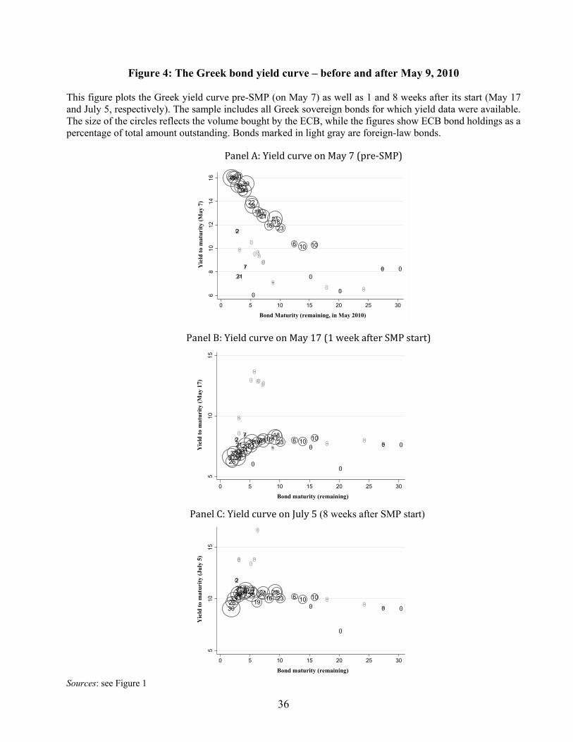
36

Figure 4: The Greek bond yield curve – before and after May 9, 2010

This figure plots the Greek yield curve pre-SMP (on May 7) as well as 1 and 8 weeks after its start (May 17 and July 5, respectively). The sample includes all Greek sovereign bonds for which yield data were available. The size of the circles reflects the volume bought by the ECB, while the figures show ECB bond holdings as a percentage of total amount outstanding. Bonds marked in light gray are foreign-law bonds.

PanelA:YieldcurveonMay7(pre‐SMP)

PanelB:YieldcurveonMay17(1weekafterSMPstart)

PanelC:YieldcurveonJuly5(8 weeks after SMP start)

Sources: see Figure 1

0

9

0

0

00

00

0 0

0

3033

3329

3824

26

36

21

34

7

22

0

1921

1621

23

31

31

18

6 10 10

0 00

0

2

68

10

12

14

16

Yie

ld t

o m

atur

ity

(May

7)

0 5 10 15 20 25 30

Bond Maturity (remaining, in May 2010)

0

9

00 00

00

0 0

0

303333

2938 24

2636

2134

7

22

0

1921162123

3131

186 10 10

0 00

0

2

51

01

5

Yie

ld t

o m

atur

ity

(May

17)

0 5 10 15 20 25 30

Bond maturity (remaining)

0

9

00

0

00

0

30

3333

2938 24

263621

347

220

19

2116

212331

31 186 10 10

0 00

0

2

51

01

5

Yie

ld t

o m

atur

ity

(Ju

ly 5

)

0 5 10 15 20 25 30

Bond maturity (remaining)

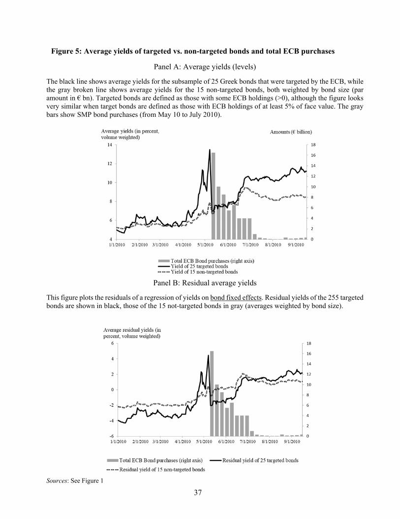
37

Figure 5: Average yields of targeted vs. non-targeted bonds and total ECB purchases

Panel A: Average yields (levels)

The black line shows average yields for the subsample of 25 Greek bonds that were targeted by the ECB, while the gray broken line shows average yields for the 15 non-targeted bonds, both weighted by bond size (par amount in € bn). Targeted bonds are defined as those with some ECB holdings (>0), although the figure looks very similar when target bonds are defined as those with ECB holdings of at least 5% of face value. The gray bars show SMP bond purchases (from May 10 to July 2010).

Panel B: Residual average yields

This figure plots the residuals of a regression of yields on bond fixed effects. Residual yields of the 255 targeted bonds are shown in black, those of the 15 not-targeted bonds in gray (averages weighted by bond size).

Sources: See Figure 1

38

Figure 6: Intra-day prices on May 10 – targeted vs. non-targeted bonds

This figure is based on high-frequency price quotes for Greek bonds from the OTC market, using the Thomson Reuters Tick History dataset. The mid-prices for May 10 are shown as 30 minute averages and computed as a ratio to the price quote at the end of the last trading day before the SMP announcement (100=closing price on May 7). The 25 bonds used here are very frequently quoted, with about 500 ticks per 30 minutes (see Panel C in Figure 7 below). The gray broken line represents averages of 5 frequently traded non-targeted bonds. The red line shows averages for 20 frequently quoted target bonds. The gray bar represents the start of SMP purchases on 09:06 a.m. The first price shown for May 10 (averages of 8:30-9:00 a.m.) can thus be interpreted as reflecting a pure announcement effect.

Sources: Thomson Reuters, authors' calculations

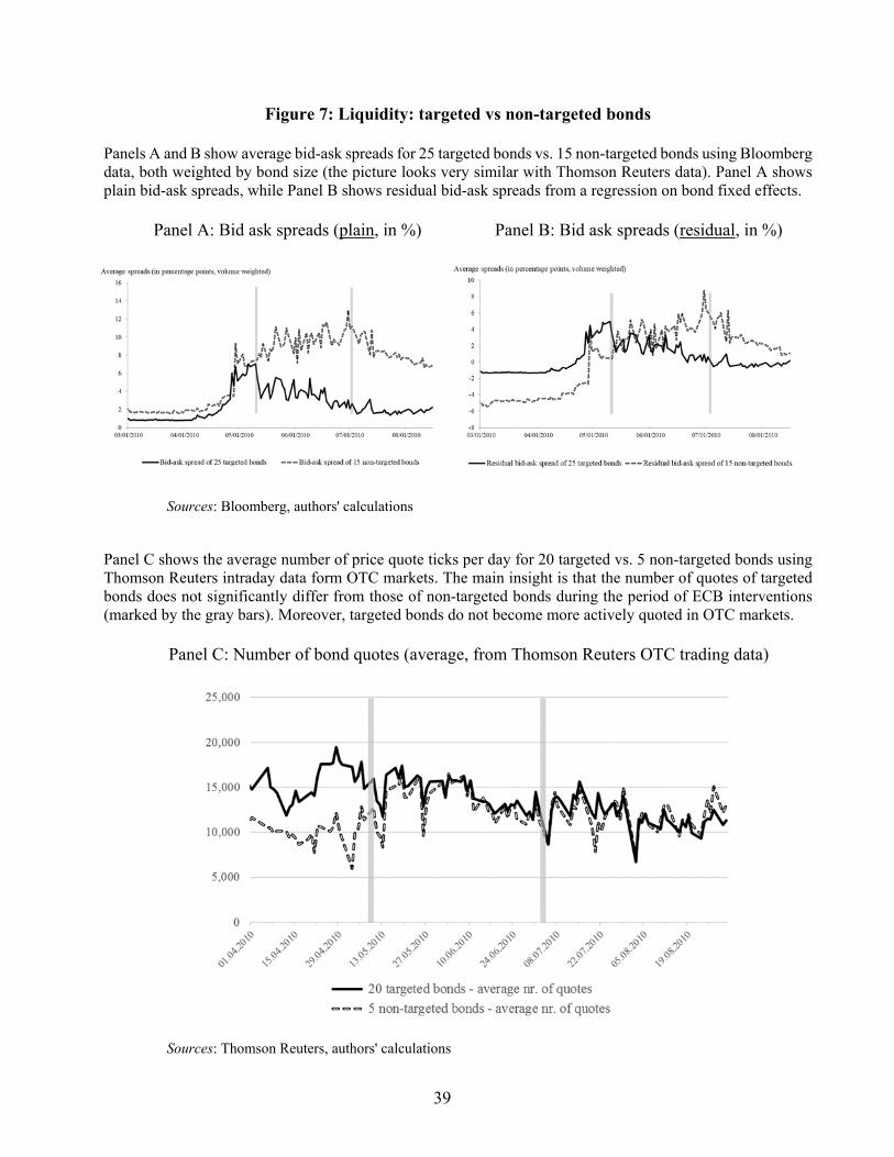
39

Figure 7: Liquidity: targeted vs non-targeted bonds

Panels A and B show average bid-ask spreads for 25 targeted bonds vs. 15 non-targeted bonds using Bloomberg data, both weighted by bond size (the picture looks very similar with Thomson Reuters data). Panel A shows plain bid-ask spreads, while Panel B shows residual bid-ask spreads from a regression on bond fixed effects.

Panel A: Bid ask spreads (plain, in %) Panel B: Bid ask spreads (residual, in %)

Sources: Bloomberg, authors' calculations

Panel C shows the average number of price quote ticks per day for 20 targeted vs. 5 non-targeted bonds using Thomson Reuters intraday data form OTC markets. The main insight is that the number of quotes of targeted bonds does not significantly differ from those of non-targeted bonds during the period of ECB interventions (marked by the gray bars). Moreover, targeted bonds do not become more actively quoted in OTC markets.

Panel C: Number of bond quotes (average, from Thomson Reuters OTC trading data)

Sources: Thomson Reuters, authors' calculations

40

Figure 8: Sovereign CDS curve and ECB purchases

Panel A and B show the relationship between ECB bond purchases and CDS premiums using Markit data for CDS of different maturities. Panel A shows CDS premiums pre-SMP (May 7) and one week and eight weeks afterwards (May 17 and July 5), as well as the amount of ECB purchases of Greek bonds in each maturity bucket. Panel B uses the same data but shows a scatter plot of purchases (in % of total amounts in each maturity bucket) and the change (decline) in CDS premiums between May 7 and July 5, analogous to Figure 3 (and using the same vertical axis scale).

Panel A: CDS yield curves in May and July 2010

Panel B: ECB purchases and changes in CDS premiums

Sources: Greek Official Government Gazette 413 V/2012, 574 V/2012, and 705 V/2012; Markit; authors' calculations

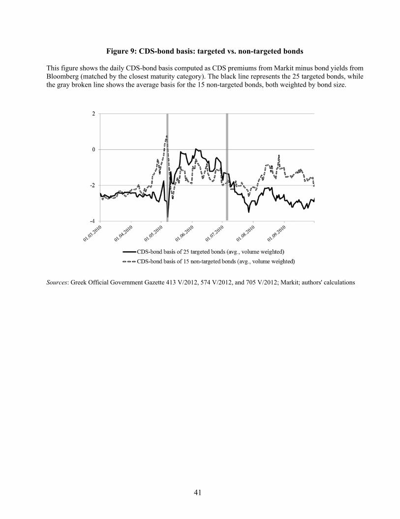
41

Figure 9: CDS-bond basis: targeted vs. non-targeted bonds

This figure shows the daily CDS-bond basis computed as CDS premiums from Markit minus bond yields from Bloomberg (matched by the closest maturity category). The black line represents the 25 targeted bonds, while the gray broken line shows the average basis for the 15 non-targeted bonds, both weighted by bond size.

Sources: Greek Official Government Gazette 413 V/2012, 574 V/2012, and 705 V/2012; Markit; authors' calculations

42

Table 1: Summary statistics of Greek government bonds

This table compares sample averages for Greek bonds bought by the ECB to the full sample of bonds (81 outstanding bonds, as used in section 3) as well as to the full sample of traded bonds (those 40 bonds priced in secondary markets, as used in section 4). All figures are Euro-weighted means.

Sources: Greek Official Government Gazette Issues 413 V/2012, 574 V/2012, and 705 V/2012, Bloomberg, Zettelmeyer et al (2013), and authors' calculations.

Average of ECB purchases

Average of 81 outstanding bonds (used in Section 3)

Average of 40 traded bonds

(used in Section 4)

Remaining maturity /1 5.4 years 9.1 years 9.1 yearsCoupon 5.0% 4.5% 4.8%Time since issued /2 3.8 years 4.0 years 4.0 years% Greek-law bonds 99.9% 92.6% 97.7%% Benchmark bonds 94.7% 74.5% 84.1%% Traded on Secondary Markets 99.8% 88.6% 100.0%Yield average (pre-SMP) /3 9.4% 8.7% 8.7%Yield increase (pre-SMP) /3 7.9% 6.3% 6.3%

/1 Remaining maturity as of May 10, 2010 (start of SMP) /2 Age of the bond as of May 10, 2010 (start of SMP) /3 The pre-SMP period are the 4 weeks between April 12 and May 7, for all bonds with yield data

This table compares sample averages for Greek bonds bought by the ECB to the full sample of bonds (all outstanding securities). All figures are Euro-weighted means.

43

Table 2: Determinants of ECB purchases This table shows results on the determinants of ECB purchases in the cross-section of Greek bonds. The dependent variable is the share of ECB purchases in each series (in % of total face value). Columns 1-6 and 8-12 show coefficients from OLS regressions, while columns 7 and 13 show coefficients of a fractional response model with a logit link function, which accounts for the fact that the dependent variable is a share bounded between 0 and 1 (following Ramalho et al. 2011). Note that the coefficients of the OLS regressions and the fractional response regressions are not directly comparable because the former, but not the latter, represent partial effects (see Woolridge 2002). Columns 1-7 are based on the full sample of 81 Greek government bonds. Columns 8-13 use the sample of 40 bonds for which yield data was available from Bloomberg. Bootstrapped standard errors are in parentheses (1000 replications, except for the FRM models in columns 7 and 13 which use regular robust standard errors). ***/**/* indicates significance at the 1%, 5%, and 10% level, respectively.

Sources: see Table 1

(1) (2) (3) (4) (5) (6) (7) (8) (9) (10) (11) (12) (13)

OLS OLS OLS OLS OLS OLS Frac OLS OLS OLS OLS OLS Frac

coef/se coef/se coef/se coef/se coef/se coef/se coef/se coef/se coef/se coef/se coef/se coef/se coef/se

1.93*** 1.21*** 0.11*** 0.59* 0.54 0.47 0.16 0.03 -0.01(0.27) (0.38) (0.04) (0.31) (0.36) (0.34) (0.40) (0.35) (0.02)

-0.41*** -0.46** -0.17*** -0.26 -0.06*(0.16) (0.22) (0.03) (0.25) (0.03)

2.94*** 1.41** 0.50*** 0.81 0.14*(0.59) (0.61) (0.10) (1.04) (0.07)

9.79*** -0.60 1.36 12.58*** 2.58**(1.92) (1.51) (0.88) (3.95) (1.09)

17.65*** 7.82* 1.24** -1.69 0.19(2.61) (4.24) (0.52) (3.66) (0.29)

7.84*** 6.37*** 0.54***

(1.17) (1.80) (0.16)

2.77***

(0.56)

3.08***(0.50)

3.98***(0.93)

0.80 10.27*** -4.86** 0.40 1.57** -0.64 -6.32*** -54.50*** -3.32 -23.78*** 11.73*** -49.02*** -9.27***(0.65) (2.21) (1.90) (0.31) (0.75) (2.54) (0.89) (8.41) (2.83) (4.57) (2.76) (12.13) (1.91)

Observations 81 81 81 81 81 81 81 40 40 40 40 40 40Adj. R2 0.451 0.055 0.163 0.153 0.484 0.629 0.76 0.719 0.588 0.661 0.573 0.794 0.88

Full Sample

Yield pre-SMP (on May 7, in %)

Bond size (amount outstanding, € bn)Remaining maturity (years, in May 2010)Coupon size (in %)

Greek law bond (Dummy)

Benchmark bond (Dummy)

Yield pre-SMP, in % (4-week average)

Constant

Yield pre-SMP (increase from April 12 to May 7)

Subsample for which yield data is available

Yield curve fitting error (on May 7, in %)

44

Table 3: Main results: cross-section

This table shows OLS regressions results in the cross-section of Greek bonds for which yield data were available. The dependent variable is the change (drop) in bond yields between Friday May 7 (before SMP start) and subsequent dates, in percentage points. The main explanatory variable captures the scope of ECB intervention, measured as the share of ECB purchases in each bond series (in % of total face value). A negative coefficient indicates that this variable is associated with a lower yield across bonds. Column 6 shows results from a two-stage least squares regression using "benchmark bond" and "coupon" as instruments for ECB bond buying shares. The variable "yield increase pre-SMP" captures the yield increase of each bond during the four weeks before the start of the SMP (from April 12 to May 7), measured in percentage points. The variable "change in CDS premiums" captures the change (drop) in CDS premiums after the start of SMP, also in percentage points. The “yield curve fitting error” captures the deviation from a smooth Nelson-Siegel-type curve estimated for May 7 (pre-SMP). Bootstrapped standard errors are shown in parentheses (1000 replications), except in the 2SLS regression which uses regular robust standard errors, corrected for small samples. ***/**/* indicates significance at the 1%, 5%, and 10% level.

Sources: Greek Official Government Gazette Issues 413 V/2012, 574 V/2012, and 705 V/2012, Bloomberg, Markit, Zettelmeyer et al (2013), and authors' calculations.

3 months (May 7 vs

Aug 6)

End-year (May 7 vs Dec. 30)

OLS OLS OLS OLS OLS 2SLS OLS OLS

(1) (2) (3) (4) (5) (6) (7) (8)

-0.10*** -0.09** -0.10*** -0.10*** -0.10*** -0.10*** -0.07*** -0.06*

(0.03) (0.04) (0.03) (0.03) (0.03) (0.04) (0.03) (0.03)

-0.16*** -0.02 -0.15*** -0.15*** -0.15*** -0.16*** -0.18*** -0.36***

(0.03) (0.04) (0.04) (0.03) (0.03) (0.03) (0.04) (0.07)

-1.27 -1.72** -1.36* -0.58 -0.56 -1.34* -0.47 -0.59

(0.78) (0.81) (0.80) (0.88) (0.89) (0.76) (0.61) (0.92)

-0.80*** -0.76*** -0.82*** -0.83*** -0.81*** -0.88*** -0.90***

(0.12) (0.13) (0.10) (0.11) (0.10) (0.13) (0.14)

-0.77***

(0.18)

0.90 -0.10 0.45 1.18**

(0.92) (0.79) (0.44) (0.55)

-0.04 -0.05

(0.04) (0.06)

7.31*** 2.41*** 7.86*** 6.44*** 6.36*** 7.32*** 7.25*** 9.95***

(0.95) (0.94) (1.19) (1.07) (1.22) (0.86) (1.27) (1.28)

F-statistic 6.43Hansen-J (p-value) 0.72

Observations 37 37 37 34 34 37 37 37

R2 (adjusted) 0.925 0.848 0.926 0.950 0.948 0.925 0.941 0.821

Greek Law Bond (Dummy)

Remaining Maturity (in years)

Change in CDS Premia (in %, by maturity)

Constant

Change in bid-ask spread (in %)

Yield curve fitting error (on May 7, in %)

Dependent Variable: Yield change after May 7…

Main results (entire first wave of SMP)

After intervention (persistence)

ECB Purchases (share of bond, in %)

Yield pre-SMP (incr. from April 12 to May 7, in %)

8 week (May 7 vs July 5)

45

Table 4: Main results: panel estimations

This table reports differences-in-differences type results from panel regressions with day fixed effects and bond fixed effects. In Columns 1-5 the dependent variable is the bond yield at market closing on each day, and the sample includes the eight weeks before and the eight weeks after the start of the SMP. In column 6 the dependent variable is the average bond yield in the 8 weeks (first time period) and 8 weeks after (second time period) the start of the SMP. CDS premiums and bid-ask spreads are similarly measured using daily levels in columns 1-5 and 8-week averages in Column 6. The main explanatory variable is a measure for ECB interventions interacted with a "Post-SMP indicator", which is 1 after the start of the SMP on May 9. ECB intervention is captured using the same measure as in Table 3, i.e. share of ECB purchases in each series. The variable "yield increase pre-SMP" captures the yield increase of each bond in the 4 weeks pre-SMP (from April 12 to May 7), in percentage points, while the “yield curve fitting error” captures the deviation from a smooth Nelson-Siegel-type curve estimated for May 7 (pre-SMP). Robust standard errors clustered by bond are reported in parentheses. ***/**/* indicates significance at the 1%, 5%, and 10% level, respectively.

Sources: see Table 3

2-period panel

(8 weeks)

(1) (2) (3) (4) (5) (6)

3.70*** 3.91*** -1.62*** 4.59*** -2.08*** -3.28**

(0.47) (0.48) (0.56) (0.40) (0.47) (1.41)

-0.11*** -0.09*** -0.11*** -0.10*** -0.10*** -0.11***

(0.02) (0.02) (0.02) (0.02) (0.02) (0.02)

0.14* 0.03 0.11 -0.00 -0.04

(0.08) (0.06) (0.07) (0.05) (0.06)

0.01(0.08)

1.51*** 1.50*** 2.56***

(0.14) (0.14) (0.63)

-0.84 1.86

(4.83) (4.18)

5.70*** 5.59*** 1.48*** 5.85*** 1.48*** -7.67**

(0.16) (0.18) (0.41) (0.17) (0.39) (3.68)

Bond fixed effects Yes Yes Yes Yes Yes Yes

Observations 3,373 3,373 3,373 3,280 3,280 74Number of bonds 40 40 40 40 40 37

Adjusted R2 0.738 0.733 0.822 0.735 0.830 0.807

Bid-ask spreads (in %)

Constant

Baseline, daily data (8-week window)

Post-SMP indicator

ECB purchases (in %) x post-SMP indicator

Yield increase pre-SMP x post-SMP indicator

Yield curve fitting error pre-SMP x post-SMP CDS premia (in %, by maturity)

46

Table 5: Spillovers and market quality effects

This table assesses the scope of spillovers and market quality effects of the ECB interventions in Greece. Columns 1 and 5 account for ECB purchases of close substitute bonds, meaning bonds within 2 years maturity of the bond's own maturity (1 year more or 1 year less), expressed as share of total bonds outstanding in the respective maturity bucket in percentage points. Columns 2 and 6 use the change and the level of bid-ask spreads as dependent variable, respectively. Columns 3 and 7 use the CDS-bond basis as dependent variable (change and level, respectively). Finally, in column 8 we show results using bond yield volatility as dependent variable, computed as the squared daily absolute change in bond yields (lagged by one day).

Sources: see Table 3

With close substitutes

Effects on bid-ask spreads

Effects on CDS-bond

basis

With close substitutes

Effects on bid-ask spreads

Effects on CDS-bond

basis

Effects on yield

volatility

Dependent variable:Change in

yieldsChange in

bid-ask spr.Change in CDS-

bond bs.Dependent variable: Yield levels

Bid-ask spreads

CDS-bond basis

Yield volatility

(1) (2) (3) (4) (5) (6) (7)

-0.20*** -0.15 0.09*** -0.12*** -0.00* 0.10*** -0.03***(0.04) (0.10) (0.03) (0.02) (0.00) (0.01) (0.01)0.02 0.01 0.02 -1.61*** 0.06*** -0.61 -0.12

(0.07) (0.23) (0.04) (0.56) (0.02) (0.41) (0.57)

-1.81* 1.59 1.78**(1.04) (3.21) (0.72)3.48** -0.40 1.39*** -0.00 0.56***(1.74) (3.01) (0.14) (0.00) (0.15)0.05 0.04**

(0.05) (0.02)

Constant 5.14*** 0.57 -4.46*** Constant 1.82*** 0.02** -2.57*** -1.54***

(1.75) (4.44) (0.79) (0.42) (0.01) (0.12) (0.45)

Observations 37 34 37 Observations 3,373 3,280 3,373 2,711

Number of bonds 37 34 37 Number of bonds 40 40 40 40Adjusted R2 0.745 0.338 0.880 Adjusted R2 0.828 0.375 0.463 0.045

Cross section (changes May 7 to July 5) Fixed effects panel (8 week window)

ECB purchases (share of bond, in %)

Post-SMP indicatorRemaining maturity (in years)

ECB purchases (in %) x post-SMP indicator

Greek law bond (Dummy)

CDS premia (in %, by maturity)

Change in CDS premia (in %, by maturity)

ECB purchases of close substitutes x post-SMP

ECB purchases of close substitutes

47

References

Acharya, Viral, Drechsler, Itamar, and Philipp Schnabl. 2014. “A Pyrrhic Victory? Bank Bailouts and Sovereign Credit Risk.” Journal of Finance, 69(6): 2689–2739.

Aguiar, Mark and Manuel Amador. 2013. "Take the Short Route: How to Repay and Restructure Sovereign Debt with Multiple Maturities." NBER Working Paper 19717.

Andritzky, Jochen, Schumacher, Julian, and Christoph Trebesch. 2014. “Total Returns in Distressed Sovereign Bond Markets.” unpublished draft. International Monetary Fund.

Arellano, Cristina and Ananth Ramanarayanan. 2012. "Default and the Maturity Structure in Sovereign Bonds." Journal of Political Economy, 120(2): 187 - 232.

Barclays. 2012. “ECB SMP: Marking to Market.” Interest Rates Research Report. 6 January 2012.

Bauer, Michael and Glenn Rudebusch. 2013. "The Signalling Channel for Federal Reserve Bond Purchases." Working Paper 2011-21. Federal Reserve Bank of San Francisco.

Beber, Alessandro, Brandt, Michael, and Kenneth Kavajecz. 2009. "Flight-to-Quality or Flight-to-Liquidity? Evidence from the Euro-Area Bond Market." Review of Financial Studies, 22(3): 925-957.

Bernanke, Ben, Reinhart, Vincent, and Brian Sack. 2004. "Monetary Policy Alternatives at the Zero Bound: An Empirical Assessment." Brookings Papers on Economic Activity, 35(2): 1-100.

Bertrand, Marianne, Duflo, Esther, and Sendhil Mullainathan. 2004. "How Much Should We Trust Differences-in-Differences Estimates?" Quarterly Journal of Economics, 119(1): 249-275.

Brunnermeier, Markus, Eisenbach, Thomas and Yuliy Sannikov. 2013. “Macroeconomics with Financial Frictions: A Survey”, in Acemoglu, Daron, Arellano, Manuel and Eddie Dekel (eds.), Advances in Economics and Econometrics, Cambridge Univ. Press, pp. 4-94.

Buchheit, Lee C., and G. Mitu Gulati. 2013. “The Gathering Storm: Contingent Liabilities in a Sovereign Debt Restructuring,” unpublished, Duke University (available on SSRN, https://papers.ssrn.com/sol3/papers.cfm?abstract_id=2292669)

Cahill, Michael, D’Amico, Stefania, Li, Canlin, and John S. Sears. 2013. “Duration Risk versus Local Supply Channel in Treasury Yields: Evidence from the Federal Reserve’s Asset Purchase Announcements.” Federal Reserve Board.

Calice, Giovanni, Chen, Jing, and Julian Williams. 2013. "Liquidity Spillovers in Sovereign Bond and CDS markets: An Analysis of the Eurozone Sovereign Debt Crisis." Journal of Economic Behavior and Organization, 85(3): 122-143.

Chen, Long, Lesmond, David, and Jason Wei. 2007. "Corporate Yield Spreads and Bond Liquidity." Journal of Finance, 62(1): 119-149.

Cruces, Juan, Buscaglia, Marcos, and Joaquin Alonso. 2002. “The Term Structure of Country Risk and Valuation in Emerging Markets.” Universidad de San Andres Working Paper 46.

D'Amico, Stefania, English, William López-Salido, David, and Edward Nelson. 2012. "The Federal Reserve’s Large-Scale Asset Purchase Programs: Rationale and Effects." Economic Journal, 122(564): 415-446.

48

D’Amico, Stefania and Thomas B. King. 2013. "Flow and Stock Effects of Large-scale Treasury Purchases: Evidence on the Importance of Local Supply." Journal of Financial Economics, 108(2): 425-448.

De Pooter, Michiel, Martin, Robert F. and Seth Pruitt. 2016. “The Liquidity Effects of Official Bond Market Intervention.” FRB International Finance Discussion Paper 1138, Board of Governors of the Federal Reserve System.

Doran, David, Dunne, Peter, Monks, Allen, and Gerard O'Reilly. 2014. "Was the Securities Markets Programme Effective in Stabilizing Irish Sovereign Yields?", unpublished (earlier version issued as Central Bank of Ireland Research Paper 07/RT/13).

Drechsler, Itamar, Dechsel, Thomas, Marquez-Ibanez, Daniel and Philipp Schnabl. 2016. “Who Borrows from the Lender of Last Resort?”Journal of Finance, 71, 1933–1974.

Duffie, Darrell, Garleanu, Nicolae, and Lasse Heje Pedersen. 2005. "Over-the-Counter Markets." Econometrica, 73(6): 1815-1847.

Duffie, Darrell, Garleanu, Nicolae, and Lasse He. Pedersen. 2007. “Valuation in Over-the-Counter Markets.” Review of Financial Studies, 20(6): 1865–1900.

Duygan-Bump, Burcu, Parkinson, Patrick, Rosengren, Eric, Suarez, Gustavo, and Paul Willen. 2013. “How Effective Were the Federal Reserve Emergency Liquidity Facilities? Evidence from the Asset-Backed Commercial Paper Money Market Mutual Fund Liquidity Facility.” Journal of Finance, 68(2): 715-737.

Eggertsson, Gauti and Michael Woodford. 2003 “The Zero Bound on Interest Rates and Optimal Monetary Policy.” Brookings Papers on Economic Activity, 34(1): 139–235.

Eser, Fabian and Bernd Schwaab. 2016. “Evaluating the Impact of Unconventional Monetary Policy Measures: Empirical Evidence from the ECB's Securities Markets Programme.” Journal of Financial Economics 119(1): 147–167.

Gagnon, Joseph, Raskin, Matthew, Remache, Julie, and Brian Sack. 2011. “Large-Scale Asset Purchases by the Federal Reserve: Did They Work?” Federal Reserve Bank of New York Economic Policy Review, May, 41-59

Ghysels, Eric, Idier, Julien, Manganelli, Simone, and Olivier Vergote. 2017. "A High Frequency Assessment of the ECB Securities Markets Programme." Journal of the European Economic Association 15(1): 218-243.

Greenwood, Robin and Dimitri Vayanos. 2010. "Price Pressure in the Government Bond Market." American Economic Review, 100(2): 585–90.

Greenwood, Robin and Dimitri Vayanos. 2014. “Bond Supply and Excess Bond Returns.” Review of Financial Studies, 27(3): 663-713.

Gürkaynak, Refet and Jonathan H. Wright. 2012. “Macroeconomics and the Term Structure.” Journal of Economic Literature, 50(2): 331-367.

Hamilton, James D. and Jing Cynthia Wu. 2012. “The Effectiveness of Alternative Monetary Policy Tools in a Zero Lower Bound Environment.” Journal of Money, Credit and Banking, 44: 3–46.

Härdle, Wolfgang Karl and Piotr Majer. 2012. "Yield Curve Modeling and Forecasting using Semiparametric Factor Dynamics." SFB 649 Discussion Paper, Humboldt University, Berlin.

Hume, Neil. 2010. “The peripheral bond buyer of last resort” FT Alphaville, December 13 2010 (http://ftalphaville.ft.com/blog/2010/12/13/434886/the-peripheral-bond-buyer-of-last-resort)

49

International Monetary Fund. 2013. “Unconventional Monetary Policies: Recent Experience and Prospects.” Special Report, April 18, 2013. (https://www.imf.org/external/np/pp/eng/2013/041813a.pdf)

Joyce, Michael, Lasaosa, Ana, Stevens, Ibrahim, and Matthew Tong. 2011. "The Financial Market Impact of Quantitative Easing in the United Kingdom." International Journal of Central Banking, 7(3): 113-161.

Joyce, Michael and Matthew Tong, 2012."QE and the Gilt Market: A Disaggregated Analysis." Economic Journal, 122(564): 348-384.

Krishnamurthy, Arvind, Nagel, Stefan, and Annette Vissing-Jorgensen. 2015. “ECB Policies involving Government Bond Purchases: Impact and Channels.” unpublished draft.

Krishnamurthy, Arvind and Annette Vissing-Jorgensen. 2011. “The Effects of Quantitative Easing on Interest Rates: Channels and Implications for Policy.” Brookings Papers on Economic Activity, Fall 2011: 215–265.

Krishnamurthy, Arvind and Annette Vissing-Jorgensen. 2012. "The Aggregate Demand for Treasury Debt." Journal of Political Economy, 120(2): 233 - 267.

Longstaff, Francis, Sanjay Mithal and Eric Neis. 2005. "Corporate Yield Spreads: Default Risk or Liquidity? New Evidence from the Credit Default Swap Market." Journal of Finance, 60(5): 2213-2253.

Mesters, Geert, Bernd Schwaab and Siem Jan Koopman. 2014. “A Dynamic Yield Curve Model with Stochastic Volatility and Non-Gaussian Interactions: An Empirical Study of Non-Standard Monetary Policy in the Euro Area.” Tinbergen Institute Discussion Paper 14-071/III.

Nelson, Rebecca M., Paul Belkin and Derek E. Mix. 2010. “Greece’s Debt Crisis: Overview, Policy Responses, and Implications.” CRS Report for Congress, Congressional Research Service (http://fpc.state.gov/documents/organization/142363.pdf).

Oehmke, Martin and Adam Zawadowski. 2014. “The Anatomy of the CDS Market.“ unpublished draft.

Papke, Leslie and Jeffrey Wooldridge. 2008. “Panel Data Methods for Fractional Response Variables with an Application to Test Pass Rates.” Journal of Econometrics, 145(1-2), 121-133.

Pelizzon, Loriana, Subrahmanyam, Marti, Tomio, Davide, and Jun Uno. 2014. “The Microstructure of the European Sovereign Bond Market: A Study of the Euro-zone Crisis.” unpublished.

Ramalho, Esmeralda, Ramalho, Joaquim, and José Murteira. 2011. “Alternative Estimating and Testing Empirical Strategies for Fractional Response Regression Models.” Journal of Economic Surveys, 25(1): 19-68

Vayanos, Dimitri and Jean-Luc Vila. 2009. "A Preferred-Habitat Model of the Term Structure of Interest Rates." NBER Working Paper 15487.

Wooldridge, Jeffrey M. 2002. Econometric Analysis of Cross-Section and Panel Data. MIT Press.

Zettelmeyer, Jeromin, Trebesch, Christoph, and Mitu Gulati. 2013. “The Greek Debt Restructuring: An Autopsy.” Economic Policy. 28(75): 513–563.

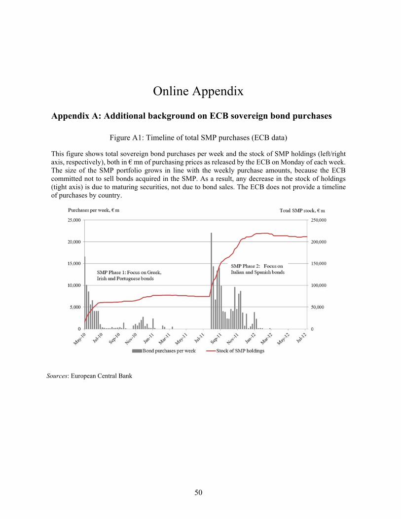
50

Online Appendix

Appendix A: Additional background on ECB sovereign bond purchases

Figure A1: Timeline of total SMP purchases (ECB data)

This figure shows total sovereign bond purchases per week and the stock of SMP holdings (left/right axis, respectively), both in € mn of purchasing prices as released by the ECB on Monday of each week. The size of the SMP portfolio grows in line with the weekly purchase amounts, because the ECB committed not to sell bonds acquired in the SMP. As a result, any decrease in the stock of holdings (tight axis) is due to maturing securities, not due to bond sales. The ECB does not provide a timeline of purchases by country.

Sources: European Central Bank

51

Box A1: Using ECB holdings data from 2012 to proxy ECB purchases in mid-2010

As explained in section 2.2., we use information from the Greek debt exchange of 2012 to proxy purchasing amounts of Greek bonds in mid-2010. We assess the validity of our approach in various ways.

One possible concern is that the data released by Greek authorities was not fully accurate. To assess this, we benchmark the data extracted from the Greek Government Gazette after the “silent swap” of February 2012 against other sources. First, we compare the sum of holdings from the gazettes to the total figure published in the official Greek debt exchange memorandum of March 2012. The memorandum explicitly states that €56.5bn “were acquired by the European Central Bank and certain National Central Banks prior to 22 February 2012” (p. 15). This figure is identical to the sum of the gazette-based holdings data of the ECB (€42.7bn), NCBs (€13.5bn), and EIB (€315mn). Second, we compare for each bond the amount of private sector holdings eligible for the exchange (from the Greek bond exchange memoranda) to the total principal amount outstanding of that bond in February (from Bloomberg). The residual is equivalent to the amount held by non-private creditors, i.e. the total holdings by the exempt ECB, NCBs, and the EIB. Again, we find the information to be coherent. The big advantage of using the gazette information compared to the Bloomberg route is that it allows us to distinguish ECB holdings (purchased via the SMP) from those of National Central Banks and the EIB holdings.

A second concern is that the ECB holdings as of February 2012 measure the amounts purchased in May and June 2010 with error. We discuss in the main paper how this could bias our estimation results and how we address measurement error in our econometric analysis. Here, we provide additional evidence on the share of February 2012 holdings that were bought in mid-2010. Figure A2 shows estimates by Barclay’s, a major dealer in Greek sovereign bonds, on the weekly purchase amounts between early May and early July 2010. Barclays estimates that the total ECB purchases in May and June 2010 were mostly targeted towards Greek bonds, and, accordingly, that the largest chunk of Greek bonds were purchased in the first few weeks of the SMP (we also have the estimated purchases in 2011 and 2012 and they are negligible in comparison). For our main period of analysis, from May 10 to July 5, Barclays estimates a total amount of Greek bond purchases of €35bn at market prices, or roughly €40bn at face value. This implies that more than 75% of total SMP purchases of Greek bonds occurred in the first 8 weeks (after May 10), after accounting for bonds maturing between mid-2010 and early 2012. These estimates by Barclays are roughly in line with the view of several market participants we talked to and also with press reporting on leaked information at the time. Most notably, in early June 2010, three weeks after the programme start, the Wall Street Journal reported that the ECB had already “spent about €25bn on Greek debt according to a senior Bundesbank official who declined to be named”, while Der Spiegel reported that “the ECB already has about €25bn of Greece's mountain of debt on its books, and it is adding another €2bn a day, on average.”54 These figures are very similar to the Barclays’ estimate of Greek bond purchases in May 2010, namely €22bn at secondary market prices or more than €26bn at face value (at an average price discount of 15%, and including maturing bonds between mid-2010 and early 2012). This would mean that more than 50% of all Greek bonds in the ECB portfolio were bought in the first three weeks of the SMP. We thus conclude that all available evidence supports the view that the February 2012 holdings are a reasonable proxy for the subset of Greek bond purchased in mid-2010.

A third and final concern regarding the ECB purchase data is that we lack purchasing amounts for bonds maturing between May 2010 and February 2012 (i.e. bonds with less than 20 months of remaining maturity in May 2010). To shed light on the scope of these omitted bonds, we checked Bloomberg and Dealogic and found four Greek sovereign bonds that matured in this period and were also trading on secondary markets. These bonds had an outstanding face value of €22bn or 11% of the total amount of Greek sovereign bonds trading on the secondary market. We found another 10 smaller bonds for which no price data was available (less than 2% of total amount outstanding).

54 See WSJ, June 1, 2010, “Bundesbank Attacks ECB Bond-Buying Plan“ and Der Spiegel, May 31, 2010, “ECB Buying Up Greek Bonds: German Central Bankers Suspect French Intrigue.”

52

Figure A2: SMP purchases of Greek bonds in 2010 (Estimates from Barclays 2012)

This figure shows estimates of weekly SMP purchasing volumes of Greek bonds in € mn of purchasing prices, taken from Barclays (2012). According to the data, the ECB purchased €35bn of Greek bonds in the first 8 weeks of the programme (from May 9 to July 5). This corresponds to €40bn at face value, or more than 75% of total ECB purchases of Greek bonds.

Sources: Barclays

53

Table A1: List of all Greek sovereign bonds and their ECB and NCBs holdings

ISIN Maturity Governing Law

Currency Exchange Total Volume Outstanding (€ mn, as of Febr. 2012)

Private Sector Holdings

(€ mn, eligible for exchange)

NCBs Holdings

(€ mn)

ECB Holdings

(€ mn)

Share of ECB

Holdings (in %)

GR0110021236 20.03.2012 Greek law EUR Athens 14435.0 9765.6 316.0 4273.2 29.6%

XS0147393861 15.05.2012 English law EUR Luxembourg 450.0 450.0 0.0 0.0 0.0%

GR0124018525 18.05.2012 Greek law EUR Athens 8000.0 4665.7 1220.3 2074.0 25.9%

GR0124020547 20.06.2012 Greek law EUR Athens 413.7 413.7 0.0 0.0 0.0%

GR0106003792 30.06.2012 Greek law EUR Athens 140.3 140.3 0.0 0.0 0.0%

GR0114020457 20.08.2012 Greek law EUR Athens 7720.0 4586.0 551.5 2517.4 32.6%

GR0326042257 22.12.2012 Greek law EUR Not Listed 2026.3 2026.3 0.0 0.0 0.0%

GR0508001121 31.12.2012 Greek law EUR Athens 22.9 22.9 0.0 0.0 0.0%

GR0512001356 20.02.2013 Greek law EUR Athens 5820.0 5376.7 302.0 121.3 2.1%

GR0110022242 31.03.2013 Greek law EUR Athens 36.4 36.4 0.0 0.0 0.0%

GR0124021552 20.05.2013 Greek law EUR Athens 9079.5 4490.6 1283.3 3288.6 36.2%

GR0128001584 20.05.2013 Greek law EUR Athens 2497.6 1492.7 225.3 779.6 31.2%

XS0372384064 25.06.2013 English law USD Frankfurt 1133.8 1083.9 49.7 0.0 0.0%

GR0124022568 03.07.2013 Greek law EUR n.a. 410.3 326.0 0.0 84.3 20.5%

CH0021839524 05.07.2013 Swiss law CHF SIX 538.4 538.4 0.0 0.0 0.0%

GR0110023257 31.07.2013 Greek law EUR Athens 64.3 64.3 0.0 0.0 0.0%

GR0114021463 20.08.2013 Greek law EUR Athens 5850.2 3680.2 268.0 1902.0 32.5%

GR0124023574 30.09.2013 Greek law EUR Athens 149.4 149.4 0.0 0.0 0.0%

GR0326043263 22.12.2013 Greek law EUR Not Listed 1854.7 1853.8 0.0 0.0 0.0%

GR0128002590 11.01.2014 Greek law EUR Athens 4552.1 2699.0 374.4 1424.8 31.3%

GR0124024580 20.05.2014 Greek law EUR Athens 8523.4 4368.7 1249.5 2868.3 33.7%

XS0097596463 21.05.2014 English law EUR Not Listed 70.0 69.0 0.0 1.0 1.4%

GR0124025595 01.07.2014 Greek law EUR Athens 424.0 394.0 0.0 30.0 7.1%

GR0112003653 25.07.2014 Greek law EUR Athens 155.4 155.4 0.0 0.0 0.0%

GR0114022479 20.08.2014 Greek law EUR Athens 12500.0 8541.2 393.0 3565.8 28.5%

GR0112004669 30.09.2014 Greek law EUR Athens 85.7 85.7 0.0 0.0 0.0%

GR0514020172 04.02.2015 Greek law EUR Athens 2020.0 2020.0 0.0 0.0 0.0%

JP530000CR76 14.07.2015 Japanese law JPY Not Listed 188.3 188.3 0.0 0.0 0.0%

GR0124026601 20.07.2015 Greek law EUR Athens 9584.9 6093.5 1360.5 2095.9 21.9%

GR0114023485 20.08.2015 Greek law EUR Athens 8000.0 4811.7 168.0 3020.3 37.8%

GR0114024491 30.09.2015 Greek law EUR Athens 171.4 171.4 0.0 0.0 0.0%

GR0124027617 10.11.2015 Greek law EUR Athens 375.0 375.0 0.0 0.0 0.0%

JP530000BS19 01.02.2016 Japanese law JPY Not Listed 282.4 282.4 0.0 0.0 0.0%

XS0165956672 08.04.2016 English law EUR Not Listed 400.0 400.0 0.0 0.0 0.0%

XS0357333029 11.04.2016 English law EUR Not Listed 5600.0 5547.2 30.0 22.8 0.4%

GR0516003606 21.05.2016 Greek law EUR Athens 170.3 170.3 0.0 0.0 0.0%

GR0124028623 20.07.2016 Greek law EUR Athens 7750.0 5442.4 821.8 1446.1 18.7%

JP530000CS83 22.08.2016 Japanese law JPY Not Listed 376.6 376.6 0.0 0.0 0.0%

GR0116002875 13.09.2016 Greek law EUR Athens 142.9 142.9 0.0 0.0 0.0%

XS0071095045 08.11.2016 English law JPY Not Listed 376.6 376.6 0.0 0.0 0.0%

GR0326038214 27.12.2016 Greek law EUR Athens 383.7 334.3 0.0 0.0 0.0%

GR0118014621 01.03.2017 Greek law EUR Not Listed 342.9 342.9 0.0 0.0 0.0%

GR0528002315 04.04.2017 Greek law EUR Athens 4985.0 4937.0 0.0 48.0 1.0%

GR0118012609 20.04.2017 Greek law EUR Athens 5000.0 3646.2 168.0 1185.8 23.7%

GR0518072922 01.07.2017 Greek law EUR Athens 415.5 415.5 0.0 0.0 0.0%

GR0518071916 01.07.2017 Greek law EUR Athens 71.6 71.6 0.0 0.0 0.0%

XS0078057725 03.07.2017 English law JPY Not Listed 282.4 282.4 0.0 0.0 0.0%

GR0124029639 20.07.2017 Greek law EUR Athens 11440.0 7562.5 1455.7 2412.2 21.1%

XS0079012166 08.08.2017 English law JPY Luxembourg 470.7 470.7 0.0 0.0 0.0%

54

Table A1 (Ct’d): List of all Greek sovereign bonds and their ECB and NCBs holdings

Sources: Greek Official Government Gazette Issues 413 V/2012, 574 V/2012, and 705 V/2012, Zettelmeyer et al (2013),

ISIN Maturity Governing Law

Currency Exchange Total Volume Outstanding (€ mn, as of Febr. 2012)

Private Sector Holdings

(€ mn, eligible for exchange)

NCBs Holdings

(€ mn)

ECB Holdings

(€ mn)

Share of ECB

Holdings (in %)

GR0118013615 09.10.2017 Greek law EUR Not Listed 214.3 214.3 0.0 0.0 0.0%

GR0120003141 03.04.2018 Greek law EUR Not Listed 444.0 440.0 0.0 0.0 0.0%

XS0260024277 05.07.2018 English law EUR Not Listed 2100.0 2086.0 0.0 14.0 0.7%

GR0124030645 20.07.2018 Greek law EUR Athens 7732.1 5875.8 590.5 1255.9 16.2%

XS0286916027 22.02.2019 English law EUR Not Listed 280.0 280.0 0.0 0.0 0.0%

GR0122002737 27.02.2019 Greek law EUR Athens 112.0 112.0 0.0 0.0 0.0%

GR0122003743 04.03.2019 Greek law EUR Not Listed 425.0 425.0 0.0 0.0 0.0%

IT0006527532 11.03.2019 Italian law EUR Milan 200.0 182.9 0.0 17.1 8.6%

XS0097010440 30.04.2019 English law JPY Not Listed 235.4 235.4 0.0 0.0 0.0%

XS0097598329 03.06.2019 English law EUR Not Listed 110.0 110.0 0.0 0.0 0.0%

GR0124031650 19.07.2019 Greek law EUR Athens 15500.0 11747.6 434.5 3318.0 21.4%

GR0120002135 17.09.2019 Greek law EUR Not Listed 350.0 350.0 0.0 0.0 0.0%

GR0133001140 22.10.2019 Greek law EUR Athens 8192.0 6175.0 561.9 1450.7 17.7%

GR0124032666 19.06.2020 Greek law EUR Athens 5000.0 3633.7 234.0 1132.4 22.6%

XS0224227313 13.07.2020 English law EUR Not Listed 250.0 250.0 0.0 0.0 0.0%

XS0251384904 19.04.2021 English law EUR Not Listed 250.0 250.0 0.0 0.0 0.0%

XS0255739350 31.05.2021 English law EUR Not Listed 100.0 100.0 0.0 0.0 0.0%

XS0256563429 09.06.2021 English law EUR Not Listed 150.0 150.0 0.0 0.0 0.0%

GR0133002155 22.10.2022 Greek law EUR Athens 8930.0 7623.3 767.9 539.3 6.0%

GR0133003161 20.03.2024 Greek law EUR Athens 10462.8 9156.9 215.0 1090.9 10.4%

XS0223870907 07.07.2024 English law EUR Not Listed 250.0 250.0 0.0 0.0 0.0%

XS0223064139 06.07.2025 English law EUR Not Listed 400.0 400.0 0.0 0.0 0.0%

GR0338001531 25.07.2025 Greek law EUR Athens 8648.4 8584.9 48.0 0.0 0.0%

GR0133004177 20.03.2026 Greek law EUR Athens 7000.0 6063.3 240.0 696.7 10.0%

XS0260349492 10.07.2026 English law EUR Not Listed 130.0 130.0 0.0 0.0 0.0%

XS0110307930 14.04.2028 English law EUR SIX 200.0 200.0 0.0 0.0 0.0%

GR0338002547 25.07.2030 Greek law EUR Athens 8344.9 8244.8 75.0 0.0 0.0%

XS0192416617 10.05.2034 English law EUR Not Listed 1000.0 1000.0 0.0 0.0 0.0%

XS0191352847 17.07.2034 English law EUR Frankfurt 1000.0 1000.0 0.0 0.0 0.0%

GR0138001673 20.09.2037 Greek law EUR Athens 9000.0 8867.2 116.0 16.8 0.2%

GR0138002689 20.09.2040 Greek law EUR Athens 7920.0 7920.0 0.0 0.0 0.0%XS0292467775 25.07.2057 English law EUR Luxembourg 1778.4 1778.4 0.0 0.0 0.0%

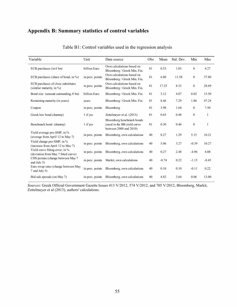
55

Appendix B: Summary statistics of control variables

Table B1: Control variables used in the regression analysis

Sources: Greek Official Government Gazette Issues 413 V/2012, 574 V/2012, and 705 V/2012, Bloomberg, Markit, Zettelmeyer et al (2013), authors' calculations.

Variable Unit Data source Obs Mean Std. Dev. Min Max

ECB purchases (in € bn) billion EuroOwn calculations based on Bloomberg / Greek Min. Fin.

81 0.53 1.03 0 4.27

ECB purchases (share of bond, in %) in perc. pointsOwn calculations based on Bloomberg / Greek Min. Fin.

81 6.80 11.58 0 37.80

ECB purchases of close substitutes (similar maturity, in %)

in perc. pointsOwn calculations based on Bloomberg / Greek Min. Fin.

81 17.25 8.33 0 28.69

Bond size (amount outstanding, € bn) billion Euro Bloomberg / Greek Min. Fin. 81 3.12 4.07 0.02 15.50

Remaining maturity (in years) years Bloomberg / Greek Min. Fin. 81 8.46 7.29 1.86 47.24

Coupon in perc. points Bloomberg 81 3.98 1.64 0 7.50

Greek law bond (dummy) 1 if yes Zettelmeyer et al. (2013) 81 0.65 0.48 0 1

Benchmark bond (dummy) 1 if yesBloomberg benchmark bonds (used in the BB yield curve between 2000 and 2010)

81 0.30 0.46 0 1

Yield average pre-SMP, in % (average from April 12 to May 7)

in perc. points Bloomberg, own calculations 40 8.27 1.29 5.15 10.21

Yield change pre-SMP, in % (increase from April 12 to May 7)

in perc. points Bloomberg, own calculations 40 5.06 3.27 -0.39 10.27

Yield curve fitting error, in % (deviation from May 7 fitted curve)

in perc. points Bloomberg, own calculations 40 0.27 2.48 -4.96 4.08

CDS premia (change between May 7 and July 5)

in perc. points Markit, own calculations 40 -0.74 0.22 -1.15 -0.45

Euro swap rates (change between May 7 and July 5)

in perc. points Bloomberg, own calculations 40 0.10 0.10 -0.11 0.22

Bid-ask spreads (on May 7) in perc. points Bloomberg, own calculations 40 4.82 3.64 0.06 13.00

56

Appendix C: Analysis of pre-SMP yields

Table C1: Correlates of pre-SMP yield increases and average yield levels

This table shows OLS regressions results in the cross-section of Greek bonds for which yield data were available. In columns (1) through (5), the dependent variable is the change (increase) in bond yields between April 12 (four weeks before SMP start) and May 7 (one day before SMP start). In columns (6) through (10), the dependent variable is the level of yields averaged over all daily observations during the four week pre-SMP period, in percentage points. The explanatory variables are the same as in Table 2. A negative coefficient indicates that this variable is associated with a smaller yield increase (columns 1-5) or lower average yield (columns 6-10) across bonds. ***/**/* indicates significance at the 1%, 5%, and 10% level, respectively.

Sources: Greek Official Government Gazette Issues 413 V/2012, 574 V/2012, and 705 V/2012, Bloomberg, Zettelmeyer et al (2013), and authors' calculations.

(1) (2) (3) (4) (5) (6) (7) (8) (9) (10)

OLS OLS OLS OLS OLS OLS OLS OLS OLS OLS

coef/se coef/se coef/se coef/se coef/se coef/se coef/se coef/se coef/se coef/se

-0.28*** -0.31*** -0.10*** -0.11***(0.06) (0.05) (0.03) (0.02)

0.36*** 0.39** 0.12*** 0.10(0.09) (0.17) (0.04) (0.07)

2.67*** 0.33 1.27*** 0.97(0.93) (1.26) (0.37) (0.72)

2.96*** -0.16 0.99*** -0.53(1.01) (1.69) (0.34) (0.75)

7.46*** 3.05*** 3.53*** 2.92*** 5.38*** 9.15*** 7.60*** 7.54*** 7.56*** 8.46***(0.74) (0.66) (0.72) (0.84) (0.69) (0.29) (0.22) (0.29) (0.24) (0.29)

Observations 40 40 40 40 40 40 40 40 40 40Adj. R2 0.347 0.223 0.146 0.145 0.638 0.299 0.153 0.223 0.097 0.561

Constant

Dependent variable: pre-SMP yield increase (change between April 12 and May 7)

Dependent variable: pre-SMP yield levels (4-week average April 12-May 7)

Remaining maturity (years, in May Bond size (amount outstanding, € bn)Benchmark bond (Dummy)Greek law bond (Dummy)

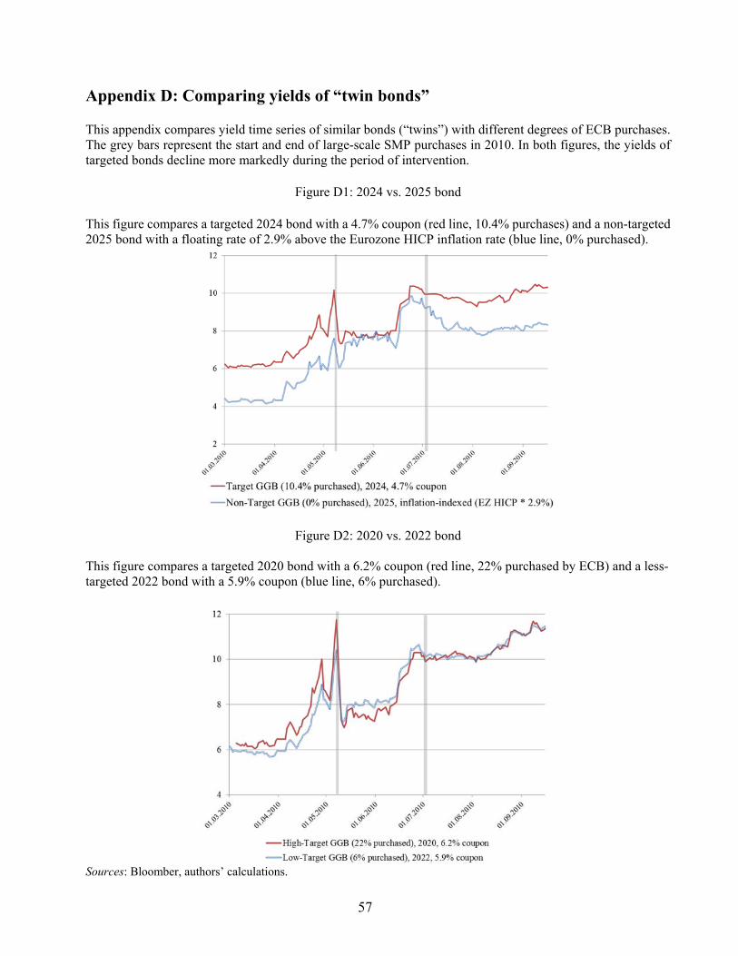
57

Appendix D: Comparing yields of “twin bonds”

This appendix compares yield time series of similar bonds (“twins”) with different degrees of ECB purchases. The grey bars represent the start and end of large-scale SMP purchases in 2010. In both figures, the yields of targeted bonds decline more markedly during the period of intervention.

Figure D1: 2024 vs. 2025 bond

This figure compares a targeted 2024 bond with a 4.7% coupon (red line, 10.4% purchases) and a non-targeted 2025 bond with a floating rate of 2.9% above the Eurozone HICP inflation rate (blue line, 0% purchased).

Figure D2: 2020 vs. 2022 bond This figure compares a targeted 2020 bond with a 6.2% coupon (red line, 22% purchased by ECB) and a less-targeted 2022 bond with a 5.9% coupon (blue line, 6% purchased).

Sources: Bloomber, authors’ calculations.

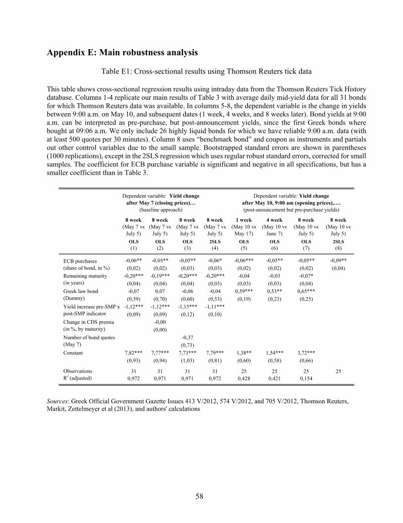
58

Appendix E: Main robustness analysis

Table E1: Cross-sectional results using Thomson Reuters tick data

This table shows cross-sectional regression results using intraday data from the Thomson Reuters Tick History database. Columns 1-4 replicate our main results of Table 3 with average daily mid-yield data for all 31 bonds for which Thomson Reuters data was available. In columns 5-8, the dependent variable is the change in yields between 9:00 a.m. on May 10, and subsequent dates (1 week, 4 weeks, and 8 weeks later). Bond yields at 9:00 a.m. can be interpreted as pre-purchase, but post-announcement yields, since the first Greek bonds where bought at 09:06 a.m. We only include 26 highly liquid bonds for which we have reliable 9:00 a.m. data (with at least 500 quotes per 30 minutes). Column 8 uses “benchmark bond” and coupon as instruments and partials out other control variables due to the small sample. Bootstrapped standard errors are shown in parentheses (1000 replications), except in the 2SLS regression which uses regular robust standard errors, corrected for small samples. The coefficient for ECB purchase variable is significant and negative in all specifications, but has a smaller coefficient than in Table 3.

Sources: Greek Official Government Gazette Issues 413 V/2012, 574 V/2012, and 705 V/2012, Thomson Reuters, Markit, Zettelmeyer et al (2013), and authors' calculations

8 week (May 7 vs

July 5)

8 week (May 7 vs

July 5)

8 week (May 7 vs

July 5)

8 week (May 7 vs

July 5)

1 week (May 10 vs

May 17)

4 week (May 10 vs

June 7)

8 week (May 10 vs

July 5)

8 week (May 10 vs

July 5)

OLS OLS OLS 2SLS OLS OLS OLS 2SLS(1) (2) (3) (4) (5) (6) (7) (8)

-0,06** -0,05** -0,05** -0,06* -0,06*** -0,05** -0,05** -0,09**

(0,02) (0,02) (0,03) (0,03) (0,02) (0,02) (0,02) (0,04)

-0,20*** -0,19*** -0,20*** -0,20*** -0,04 -0,03 -0,07*

(0,04) (0,04) (0,04) (0,03) (0,03) (0,03) (0,04)

-0,07 0,07 -0,06 -0,04 0,59*** 0,53** 0,65***

(0,59) (0,70) (0,60) (0,53) (0,19) (0,23) (0,25)

-1,12*** -1,12*** -1,15*** -1,11***

(0,09) (0,09) (0,12) (0,10)

-0,00

(0,00)

-0,37

(0,73)

7,82*** 7,77*** 7,73*** 7,79*** 1,38** 1,54*** 3,72***

(0,93) (0,94) (1,03) (0,81) (0,60) (0,58) (0,66)

Observations 31 31 31 31 25 25 25 25R2 (adjusted) 0,972 0,971 0,971 0,972 0,428 0,421 0,154

Dependent variable: Yield change after May 7 (closing prices)…

(baseline approach)

Dependent variable: Yield change after May 10, 9:00 am (opening prices),…. (post-anouncement but pre-purchase yields)

Constant

Yield increase pre-SMP x post-SMP indicator

Number of bond quotes (May 7)

Change in CDS premia (in %, by maturity)

ECB purchases (share of bond, in %)

Remaining maturity (in years)

Greek law bond (Dummy)

59

Table E2: Robustness – cross-section on the effects of bond purchases

This table expands our cross-sectional analysis of Table 3. Column 1 shows results from quantile (median) regression. Column 2 controls for the yield level on May 7 (just prior to the SMP inception), instead of using the yield increase or yield curve fitting error. Columns 3-5 show results for shorter time windows. Column 6 uses an alternative instrument, namely the yield curve fitting error pre-SMP (deviation from a smooth Nelson-Siegel-type curve estimated for May 7). The instrument is strong, as suggested by the high F-test statistic, but the Hansen J test statistic clearly rejects the null of a valid instrument. Column 7 uses yield spreads (above German Bunds) as dependent variable (in percentage points). Column 8 controls for the change in Euro area interest rate swap rates at different maturities (in percentage points). Column 9 excludes all foreign-law bonds from the regression, while Column 10 excludes floating rate bonds. Column 11 uses the total bond return as dependent variable, where the price was normalized to 100 on May 7 (pre-SMP). Bootstrapped standard errors in parentheses (1000 replications), except column 6 which shows regular robust standard errors. ***/**/* indicates significance at the 1%, 5%, and 10% level.

Sources: Greek Official Government Gazette Issues 413 V/2012, 574 V/2012, and 705 V/2012, Bloomberg, Markit, Zettelmeyer et al (2013), and authors' calculations.

Median regression

With yield level

Alternative Instrument

Yield spreads

With Euro interets

rate swaps

Greek-law bonds only

Without floating

rate bonds

Total Return

8 week (July 5)

8 week (July 5)

1 day (May 7 vs May 10)

1 week (May 7 vs May 17)

4 week (May 7 vs

June 7)

8 week (July 5)

8 week (July 5)

8 week (July 5)

8 week (July 5)

8 week (July 5)

8 week (July 5)

Quantile regression

OLS OLS OLS OLS 2SLS OLS OLS OLS OLS OLS

(1) (2) (3) (4) (5) (6) (7) (8) (9) (10) (11)

-0,07** -0,07** -0,09*** -0,10** -0,09*** -0,12*** -0,10*** -0,10*** -0,05* -0,10*** 0,34**

(0,04) (0,03) (0,02) (0,04) (0,02) (0,03) (0,03) (0,03) (0,03) (0,04) (0,14)

-0,15*** -0,13*** -0,06* -0,17** -0,13** -0,16*** -0,14*** -0,15*** -0,12*** -0,15*** 0,19

(0,04) (0,05) (0,03) (0,07) (0,05) (0,03) (0,04) (0,04) (0,03) (0,05) (0,17)

-1,33 -1,90** -0,64 -2,05** -1,70** -1,20* -1,36* -1,38* -1,40 8,60***

(1,09) (0,78) (0,56) (0,99) (0,69) (0,66) (0,78) (0,75) (0,90) (3,17)

0,33 1,30 0,45 1,26** 0,74 0,90 1,17 1,26 0,20 0,95 12,65***

(0,98) (0,94) (0,47) (0,58) (0,45) (0,84) (0,89) (1,30) (0,60) (1,00) (4,33)

-0,84*** -0,73*** -0,73*** -0,82*** -0,74*** -0,77*** -0,77*** -0,96*** -0,77*** 3,07***

(0,14) (0,13) (0,19) (0,10) (0,12) (0,13) (0,13) (0,09) (0,16) (0,55)

-0,83***

(0,15)

-0,97

(3,10)

7,39*** 13,32*** 3,75** 8,93*** 6,50*** 7,83*** 8,16*** 8,21*** 5,77*** 7,88*** -15,85***(1,43) (1,77) (1,59) (2,06) (1,38) (1,07) (1,16) (1,30) (0,61) (1,19) (4,05)

F-statistic 20,84Hansen-J (p-value) 0,00

Observations 37 37 40 40 37 37 37 37 29 35 37

R2 (adjusted) 0,920 0,950 0,913 0,955 0,925 0,928 0,923 0,971 0,924 0,881

Earlier dates (May and June)

Euro interest rate swaps (change, in %, by maturity)

Constant

ECB purchases (share of bond, in %)

Remaining maturity (in years)

Greek law bond (Dummy)

Change in CDS premia (in %, by maturity)

Yield pre-SMP (increase from April 12 to May 7, in %)

Yield level pre-SMP (on May 7, in %)

60

Table E3: Robustness – panel estimations on the effects of bond purchases This table expands the differences-in-differences type results of Table 4 on the effect of ECB bond purchases on bond yield levels (in percentage points). Columns 1 and 2 show results for shorter treatment windows (1 week and 4 weeks, respectively). Column 3 shows results using an alternative intervention measure, namely a dummy variable expressing whether the bond was targeted by the SMP or not. Column 4 uses yield spreads above German bunds as dependent variable. Column 5 controls for Euro area interest rate swap rates at different maturities (in percentage points). Column 6 excludes all foreign-law bonds from the regression, while column 7 excludes floating rate bonds. Column 8 uses total returns as dependent variable, where returns are indexed to 100 on May 7 (pre-SMP). Column 9 uses daily average yield data from the Thomson Reuters Tick History database (the results are very similar when using only the 25 highly liquid bonds of columns 5-8 in Table E1). The post-SMP indicator is a dummy that is 1 after the start of the SMP on May 9. The ECB purchase variable is the share of ECB purchases in each bond series. Robust standard errors clustered by bond are reported in parentheses. ***/**/* indicates significance at the 1%, 5%, and 10% level, respectively.

Sources: Greek Official Government Gazette Issues 413 V/2012, 574 V/2012, and 705 V/2012, Bloomberg, Thomson Reuters, Markit, Zettelmeyer et al (2013), and authors' calculations.

1-week window

4-week window

Target dummy

Yield spreads

With Euro interest

rate swaps

Greek-law bonds

only

Without floating

rate bonds

Total returns

Thomson data

(1) (2) (3) (4) (5) (6) (7) (8) (9)

1.74*** 4.15*** -0.88 -1.06* -1.18 2.09*** -1.81*** -19.05*** 3.10***

(0.60) (0.88) (0.71) (0.55) (1.04) (0.71) (0.57) (5.70) (0.88)-0.09*** -0.12*** -2.14*** -0.11*** -0.11*** -0.04*** -0.12*** 0.55*** -0.09***

(0.02) (0.02) (0.47) (0.02) (0.02) (0.01) (0.02) (0.15) (0.03)0.52*** 1.37*** 1.49*** 1.51*** 1.48*** 1.24*** 1.57*** 1.56 1.55***

(0.16) (0.22) (0.15) (0.14) (0.17) (0.16) (0.14) (1.45) (0.16)

-0.43*** -0.06 -0.15*** 0.03 0.02 -0.12** 0.04 0.30 0.01

(0.07) (0.07) (0.05) (0.06) (0.05) (0.06) (0.07) (0.44) (0.11)

0.79

(1.43)

0.00

(0.00)

6.44*** -1.58 1.53** -1.11*** -0.61 0.24 1.39*** 21.07*** -1.80

(1.51) (1.94) (0.42) (0.40) (3.66) (1.35) (0.40) (2.99) (1.25)

Bond & time fixed effects Yes Yes Yes Yes Yes Yes Yes Yes Yes

Observations 440 1,693 3,373 3,373 3,373 2,509 3,199 3,480 2,372Number of bonds 40 40 40 40 40 40 40 40 31

Adjusted R2 0.838 0.682 0.808 0.846 0.822 0.890 0.819 0.501 0.852

Constant

/1 Either share of ECB purchases in each series (in % of total face value, Columns 1-2; 4-19) or target dummy variable (Column 3)

Post-SMP indicator

ECB intervention x post-SMP indicator \1

CDS premia (in %, by maturity)

Yield increase pre-SMP x post-SMP indicator

Euro interest rate swaps (in %, by maturity)

Number of bond quotes per day

61

Appendix F: Additional robustness analysis: “placebo” regressions One way to address the concern that our results are an artefact of mean reversion, we checked whether there were other instances of large yield reversals during 2009-2012. One can then run placebo regressions to see whether the yield drop experienced by bonds purchased by the ECB in May-June 2010 differed for that of bonds that were not purchased, in spite of the fact that no intervention occurred around these alternative dates. Figure F1 shows one large yield drop similar to that on May 10, 2010, namely after the announcement of the 2nd Greek bailout on July 21, 2011, when the EU and IMF promised the Greek government financing in the amount of €109bn. Another potentially relevant event in this period is the announcement of the second wave of large-scale ECB bond buying on August 8, 2011. Table F1 shows the results from a “placebo” test using the same difference-in-difference approach as in Table 4, but centering the treatment on July 21, 2011 (2nd Greek bailout) and August 8, 2011 (2nd wave of ECB bond buying, which did not imply significant purchases of Greek bonds). We find that the ECB bond buying coefficient is statistically insignificant for various time windows around these two events. The cross-sectional data confirm this picture, since the correlation between ECB purchases and yield changes is much less pronounced compared to our main 2010 event (see Figure F2).

Figure F1: Greek bond yields 2009-2011 (average, from Bloomberg)

Sources: Greek Official Government Gazette Issues 413 V/2012, 574 V/2012, and 705 V/2012, Bloomberg, Markit, Zettelmeyer et al (2013), and authors' calculations.

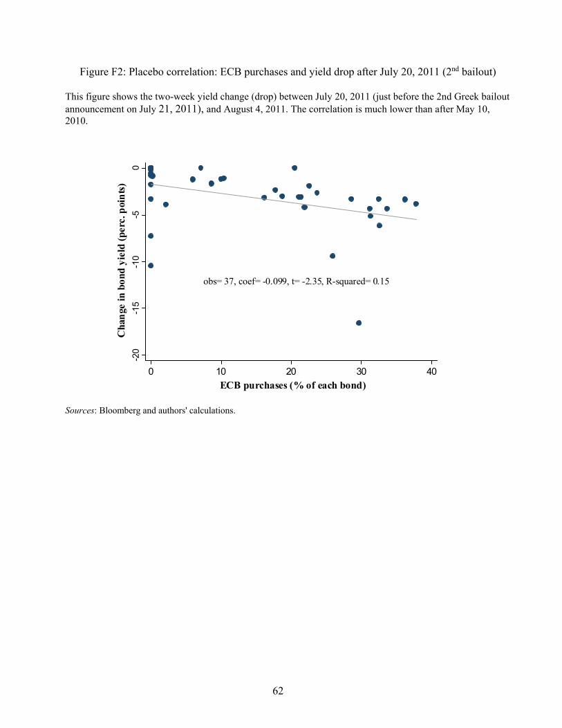
62

Figure F2: Placebo correlation: ECB purchases and yield drop after July 20, 2011 (2nd bailout)

This figure shows the two-week yield change (drop) between July 20, 2011 (just before the 2nd Greek bailout announcement on July 21, 2011), and August 4, 2011. The correlation is much lower than after May 10, 2010.

Sources: Bloomberg and authors' calculations.

obs= 37, coef= -0.099, t= -2.35, R-squared= 0.15

-20

-15

-10

-50

Cha

nge

in b

ond

yiel

d (p

erc.

poi

nts

)

0 10 20 30 40

ECB purchases (% of each bond)

63

Table F1: Placebo regressions in July and August 2011

This table shows results from placebo regressions for two central dates of the Eurozone debt crisis in 2011 that do not involve large-scale purchases of Greek bonds. First, the announcement of the 2nd Greek bailout on July 21, 2011, when the official sector (EU and IMF together) promised the Greek government financing in the amount of €109bn. Second, the start of the second wave of SMP purchases, which was announced on August 8, 2011, and continued on a large scale for about 10 weeks. We use the same difference-in-difference type regression approach as in Tables 4 and D2, but focus on these two events instead. We again include bond and day fixed effects as well as CDS premiums and for pre-event yields on July 20 and August 7, respectively. Robust standard errors clustered by bond are reported in parentheses. ***/**/* indicates significance at the 1%, 5%, and 10% level, respectively. Our main coefficient of interest (ECB purchases in each bond series) is an insignificant predictor of yield movements following these two events.

Sources: Greek Official Government Gazette Issues 413 V/2012, 574 V/2012, and 705 V/2012, Bloomberg, Markit, Zettelmeyer et al (2013), and authors' calculations

1-week window

2-week window

4-week window

1-week window

4-week window

10-week window (end of

2nd wave)

(1) (2) (3) (4) (5) (6)

5.73 14.56*** -9.71*** -0.73** -5.66*** -5.66***(4.10) (5.01) (1.59) (0.35) (0.85) (0.85)-0.04 -0.04 -0.05 -0.01 0.04 0.04

(0.03) (0.04) (0.04) (0.02) (0.04) (0.04)

-0.16*** 0.02 0.18*** 0.07*** 0.17*** 0.17***

(0.03) (0.04) (0.04) (0.03) (0.07) (0.07)

0.68 1.80*** 2.27*** -0.11 1.11*** 1.11***(0.51) (0.55) (0.43) (0.11) (0.36) (0.36)5.54 -24.40* -23.23*** 22.03*** -6.05 -6.05

(13.41) (14.26) (8.17) (1.94) (9.29) (9.29)

Bond & time fixed effects Yes Yes Yes Yes Yes Yes

Observations 407 777 1,480 407 1,511 1,511Number of bonds 37 37 37 37 37 37Adjusted R2 0.601 0.401 0.406 0.451 0.579 0.579

Constant

2nd Greek Bailout, July 21, 2011

2nd Wave of SMP Purchases, after August 8, 2011

Post-event dummy

ECB purchases (in %) x post-event dummy

CDS premia (in %, by maturity)

Pre-event yield x post-event dummy

64

Appendix G: Spillovers of ECB government bond purchases to other markets

Figure G1: Spillovers to corporate bonds

This figure shows average daily bond yields for all Greek corporations for which we could find data on Bloomberg or Thomson Reuters in mid-2010. This includes two bonds by OTE Hellenic Telecom (maturing in 2015 and 2016), one by Coca Cola Hellenic Bottling Corp. (maturing in 2016), one by Public Power Corporation PLC (maturing in Nov. 2011), as well as three bonds by banks, namely Eurobank Ergasias (maturing in 2017), National Bank of Greece (maturing in 2016), and Piraeus Bank (maturing in Sept. 2011).

Sources: Bloomberg, Thomson Reuters, and authors' calculations

65

Figure G2: Greek CDS quote data quality – sovereign vs. corporate This figure shows a proxy for the quality of CDS quotes on Greek sovereign and corporate bonds. We use daily CDS quote quality ratings by Markit, which range from a minimum of CCC to a maximum of AAA. We recode these to a numerical scale rating from 1 (CCC) to 7 (AAA) and then add up the sum of ratings over the entire maturity curve (i.e. for 6 months, 1, 2, 3, 4, 5, 7, 10, 15, 20, 30 year CDS). The resulting maximum total curve rating is 77, which is achieved when the best rating is given for CDS quotes in each of the 11 maturity categories. The orange line shows ratings for the sovereign CDS curve. The blue line shows averages for all Greek corporations for which Markit had CDS data (3 banks and 2 other): Piraeus Bank, Alpha Bank, OTE Hellenic Telecom, Eurobank Ergasias, and the Coca Cola Hellenic Bottling Corp. Only Euro-denominated CDS are considered.

Sources: Markit and authors' calculations