Working Paper 04-49 Economics Series 19 October 2004

Departamento de Economía Universidad Carlos III de Madrid

Calle Madrid, 126 28903 Getafe (Spain)

Fax (34) 91 624 98 75

EXCLUSIVE DEALING AND COMPATIBILITY OF INVESTMENTS*

Chrysovalantou Milliou1

Abstract

We examine a final product manufacturer's incentives to engage in exclusive dealing with an

input supplier when both market sides invest in quality and bargain over their trading terms.

Taking into account that the investments' compatibility can be higher under exclusive

dealing we find, in contrast to previous literature, that bargaining power distribution plays a

crucial role both for investment incentives and for incentives to adopt exclusive dealing. We

also find that there exist cases in which although investments are higher under exclusive

dealing, the manufacturer chooses non-exclusive dealing. Our welfare analysis indicates that

the manufacturer's choice of exclusive dealing in equilibrium is never welfare detrimental.

JEL Classification: L22; L42; L14; L15 Keywords: Exclusive Dealing; Supply Chains; Quality-enhancing Investments; Compatibility; Bargaining

* I am grateful to Massimo Motta, Emmanuel Petrakis, and Karl Schlag for valuable comments and discussions. I thank Yeon-Koo Che, Vincenzo Denicoló, Carlos Ponce, József Sákovics, and Margaret Slade for helpful suggestions. Full responsibility for all shortcomings is mine. 1 Department of Economics, Universidad Carlos III de Madrid, Getafe (Madrid) 28903, Spain. E-mail: cmilliou@eco.uc3m.es.

1 Introduction

In a world in which technology has considerably reduced transaction and search costs, firms

would have been expected to shop around among various suppliers for the best deal. In

contrast to this expectation, there is growing evidence that large manufacturing firms, such

as IBM, John Deere & Co., and Harley-Davidson, do not tend to do so.1 They tend,

instead, to restrict upstream competition by developing exclusive partnerships with their

input suppliers.2

One of the arguments commonly used to explain this trend is that firms are placing an

increased emphasis on product quality and that their dealing with a single supplier enables

them to develop tighter relations that result in better coordination of their investments in

product quality. In fact, several field studies of buyer-supplier relations have demonstrated

the advantages that smaller and tighter supplier networks have in quality and respon-

siveness, as well as in innovation and information exchange.3 For example, according to a

survey paper on the car-manufacturing industry, exclusive suppliers provide their costumers

with detailed information about their processes and products and this "information helps

automakers ensure that their component designs are compatible with suppliers’ processes,

thus improving productivity and quality."4

In this paper, we investigate the incentives of a final product manufacturer to develop an

exclusive dealing relation with an input supplier, taking the above argument into account.

To do so, we consider a simple environment in which a downstream monopolist - an input

buyer - decides at the outset whether or not it will offer an exclusive dealing contract to

one of two potential input suppliers. Both the buyer and the suppliers invest in the quality

improvement of their products before bargaining over the terms of a non-linear contract.

In order to capture the better coordination of the buyer’s and the supplier’s investments

1See e.g., Moore et al. (2002), Cusumano and Takeishi (1991), Helper (1991), as well as “Who’s morepassionate about Harley-Davidson than its motorcycle riders? The tight knit members of its $1 billion supplychain,” Forbes, 09/10/2001, and “Deer takes a giant leap,” Purchasing, 09/06/2001.

2E.g., "IBM used to have a couple dozen mechanical and cabel suppliers; now it has one for each com-modity" in “Reinventining purchasing wins the medal for big blue,” Purchasing, 09/09/1999.

3See e.g., Cusumano and Takeishi (1991), Helper (1991), and Helper and Sako (1995). According toMoore et al. (2002, p.158): "When it comes to establishing closer ties with suppliers, Tennant [a leader inmanufacturing cleaning machineries] has discovered that two is more than enough company, three a definitecrowd, and has come to prefer single-sourcing in most instances."

4See Helper and Sako (1995, p. 79).

under exclusive than under non-exclusive dealing, we assume that the compatibility of their

investments is full only in the former case.5

According to our first main result not only the compatibility of investments, but also

the bargaining power distribution plays an important role for investment incentives. De-

spite the fact that the compatibility of investments is full only under exclusive dealing,

investments are higher under exclusive than under non-exclusive relations only when the

buyer’s bargaining power is sufficiently high. Otherwise, both the buyer’s and the supplier’s

investments are higher under non-exclusive dealing. Why is this so? Under non-exclusive

dealing, the buyer does not enjoy the full compatibility of its investments, but it enjoys a

compensation for its ‘outside option’, that is, for having the option to deal with an alter-

native supplier. While the lack of full compatibility has a negative impact on the buyer’s

investment incentives, its compensation for the outside option has a positive impact as its

investments augment the outside option’s value. When the buyer’s bargaining power is low,

the ‘outside option effect’ dominates because the buyer retains a larger share of its outside

option. Strategic complementarity between the buyer’s and the supplier’s investments leads

to a similar behavior of the supplier’s investments.

Our second main result refers to the equilibrium supply chain structure. We find that ex-

clusive buyer-supplier relations arise in equilibrium whenever the buyer’s bargaining power

is high enough. This is intuitive since as we mentioned above the quality-enhancing in-

vestments behave in a similar way. What is though less intuitive is that there exist cases

in which although the investments are higher under exclusive dealing, the buyer chooses

non-exclusive dealing. In other words, the quality-enhancing investments are not the only

force at work. The buyer’s decision is also affected by the fact that competition among

the suppliers is present only in the case of non-exclusive dealing. Due to the suppliers’

competition, the buyer has effectively higher bargaining power during the contract terms

negotiations under non-exclusive dealing than under exclusive dealing where the outside

option is absent.

Our welfare analysis reveals, first, that the manufacturer’s choice of exclusive dealing

in equilibrium is never detrimental to welfare. And, second, that there exist circumstances

in which although welfare is higher under exclusive dealing, the manufacturer chooses not

5 In Section 6, we relax this assumption and endogenize the compatibility of investments.

2

to engage in an exclusive dealing relation. Therefore, from an antitrust policy’s perspec-

tive, although our results indicate that the social and the private incentives do not always

coincide, they still provide an argument against the view that exclusive dealing is an anti-

competitive practice, in the cases at least that exclusive dealing is initiated by downstream

manufacturers.

Extending our model by endogenizing the compatibility of investments, we provide con-

ditions under which our assumption regarding compatibility holds, that is, we provide con-

ditions under which compatibility turns out to be full only in the case of exclusive dealing.

In particular, we show that this can happen when the buyer’s bargaining power is suffi-

ciently high. The main force that drives this result is the following. Under non-exclusive

dealing, a supplier has lower incentives to increase the compatibility of its investments with

those of the buyer, through opening a specific research line for the buyer, because the higher

compatibility leads to higher buyer’s investments and thus to a higher value of the outside

option for which the supplier has to compensate the powerful buyer.

The impact of exclusive contracts on investment incentives was first studied by Segal

and Whinston (2000).6 Using a cooperative bargaining framework, they show that exclu-

sivity has a positive impact on investment incentives when investments are “external” ( i.e.

when they increase the value of trade with a third firm), and no impact whatsoever when

investments are “internal”. Segal and Whinston (2000) differ from us not only because

they model bargaining in a cooperative way, but, more importantly, because they do not

consider the role of the compatibility of investments. Two more recent papers by De Meza

and Selvaggi (2003) and Che and Sákovics (2004) also examined the impact of exclusivity

on investments. These papers, however, do not allow both the buyer and the suppliers to

undertake investments, and they too do not take into account the compatibility of invest-

ments. Note that in contrast to our paper, Segal and Whinston (2000) as well as De Meza

and Selvaggi (2003) and Che and Sákovics (2004) have not identified the crucial role of the

bargaining power distribution for the investment incentives.

The incentives to adopt exclusive dealing, both in the presence and in the absence of

6For an informal discussion of the potential impact of exclusivity on investments see e.g., Klein (1988), andKlein et al. (1978). For an in depth analysis of firms’ incentives to undertake noncontractible investmentsin only bilateral monopoly settings see e.g., Williamson (1985), Tirole (1986), Grossman and Hart (1986),Hart and Moore (1988), Che and Sákovics (2004a).

3

investments, have been analyzed by the vertical restraints literature (see e.g., Marvel, 1982,

Besanko and Perry, 1993, Bernheim and Whinston, 1998). In contrast to us, most of this

literature has analyzed the supplier’s, and not the buyer’s, decision regarding exclusive

dealing, and has not considered the role of bargaining in this decision. Moreover, while the

vertical restraints literature on exclusive dealing has focused on settings in which under non-

exclusive dealing, the buyers are multi-product retailers that sell the competing products

of all the suppliers, we focus on settings in which the buyer is always a single-product firm.

Undoubtedly this literature has shed some light on the antitrust issues arising in cases with

supplier-initiated exclusive contracts, but has not examined the antitrust implications of

buyer-initiated exclusive contracts.

The rest of the paper is organized as follows. We describe our model in Section 2. We

analyze the non-exclusive dealing case in Section 3 and the exclusive dealing case, along

with the impact of exclusivity on investments, in Section 4. In Section 5, we consider the

buyer’s decision regarding exclusive dealing and examine its welfare implications. In Section

6, we extend the model by endogenizing the compatibility of investments. We conclude and

discuss possible extensions in Section 7. All the proofs are included in the Appendix.

2 The Model

We consider an industry consisting of a downstream firm - input buyer, denoted by B,

and two upstream firms - potential input suppliers, each denoted by Si, with i = 1, 2.7

We assume that there is an one-to-one relation between the input and the final product

produced by the buyer, and that each input supplier faces a constant marginal cost of

production c ≥ 0.

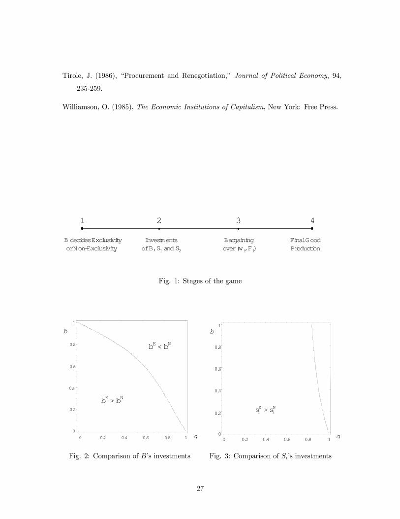
We analyze a full information four-stage game (see Fig. 1). In stage one, the buyer

decides whether or not it will engage in an exclusive relation with one of the suppliers. The

exclusive relation can be established through the use of an exclusive dealing contract that

specifies a prohibitive compensation that the buyer must pay to its exclusive supplier in

case it obtains the input from the non-exclusive supplier.

7As it will become clear later, the same results would have been obtained in a model with n suppliers,where n ≥ 2.

4

In stage two, the buyer B and its potential suppliers S1 and S2 simultaneously and inde-

pendently choose their investment levels, b, s1, and s2 respectively. Each firm’s investments

lead to an increase in the quality of its own product. We assume that the higher is the

quality of the input used in the final product, the higher is the latter’s quality. Moreover,

we assume that consumers have a higher willingness to pay for products of higher quality.

In particular, the inverse demand function for the final product is:

p = a+ bθ(b+ si)− q (1)

where a > c and q and p are respectively the quantity and the price of the final product.

The subscript i, i = 1, 2, indicates the supplier from which the buyer obtains the input.

The parameter bθ captures the degree of compatibility of the buyer’s and its input supplier’sinvestments. Low values of bθ reflect low compatibility of the outcomes of their research

projects (e.g., bad matching due to lack of coordination). We assume that compatibility is

full only under exclusive dealing. In particular, bθ = 1 under exclusive dealing and bθ = θ,

with 0 ≤ θ < 1, under non-exclusive dealing. The investments of both the buyer and the

suppliers are subject to diminishing returns to scale, captured by the quadratic form of

their cost functions: b2/2 and s2i /2.

In stage three, non-cooperative bargaining over a two-part tariff contract, consisting of

a wholesale price wi and a franchise fee Fi, takes place among the buyer and its potential

input suppliers. While under exclusive dealing the buyer bargains only with its exclusive

supplier, under non-exclusive dealing it bargains simultaneously with both S1 and S2. In

modeling the bargaining game, we adopt the approach used by De Fraja and Sákovics (2001),

Chemla (2003), Rey and Tirole (2003), and Che and Sákovics (2004).8 In particular, in the

exclusive dealing case, a take-it-or-leave-it offer over wi and Fi is made with probability β

by the exclusive supplier Si and with probability 1− β by the buyer. Similarly, in the non-exclusive dealing case, take-it-or-leave-it offers over wi and Fi, are made simultaneously and

independently by S1 and S2 with probability β and with probability 1 − β by the buyer.9

8We would have obtained exactly the same results if we had instead employed the Nash bargainingsolution.

9Similarly to the paper by De Fraja and Sákovics (2001) when the buyer makes the offer, after observingthe quality levels of both suppliers, it chooses one of the suppliers to which it makes the offer.

5

The parameter β, with 0 < β < 1, denotes the supplier’s bargaining power.

Finally, in stage four, the buyer chooses the quantity of its final good and produces it

using the input obtained according to the terms of trade specified in the previous stage.

We derive the subgame perfect Nash equilibria in pure strategies of the above four-

stage game. Since the upstream firms are identical, there are two second-stage subgames to

consider, the subgame with non-exclusive dealing and the subgame with exclusive dealing.

In what follows, we start by analyzing the two subgames separately and then move to the

analysis of stage one.

3 Non-Exclusive Dealing

In this section, we deal with the case in which the buyer is free to obtain its input from any

of the two suppliers.

In stage four, the buyer chooses the quantity that maximizes its gross profits:

Maxq

πB(q, wi, b, si) = [a+ θ(b+ si)− q −wi] q, (2)

where the subscript i, i = 1, 2, simply specifies the supplier from which the buyer obtains

its input.10 From the first order condition of (2), we obtain the equilibrium quantity:

q(wi, b, si) =a+ θ(b+ si)−wi

2. (3)

In stage three, where the bargaining takes place simultaneously among the buyer and its

potential suppliers, we distinguish among the following two cases, for i, j = 1, 2 and i 6= j:

(a) si = sj ≥ 0: When the suppliers offer the same input quality, competition among

them results not only in both of them making the same offer, but also in making an offer

that leaves them with zero profits. Formally, each Si makes an offer that maximizes the

10We assume w.l.o.g. that the buyer always buys all its input quantity from one supplier. When the buyeris indifferent between purchasing from any one of the two suppliers, we can distinguish among two cases:(1) if the suppliers offer different input qualities, the buyer will always buy from the high quality supplier —this is a reasonable tie-breaking rule, and (2) if the two suppliers offer the same input quality and the sameterms of trade, it makes no difference for our analysis if the buyer buys all the input quantity from one ofthem or if it splits this quantity between the two in any arbitrary way. Perry and Sákovics (2003) show thatwith a fixed number of suppliers the buyer prefers a sole-source auction to a split-award auction.

6

buyer’s profits subject to the constraint that its own profits are non-negative:

Maxwi,Fi

[q(wi, b, si)]2 − Fi s.t. (wi − c)q(wi, b, si) + Fi ≥ 0. (4)

The constraint in (4) is binding, and thus, the supplier’s maximization problem becomes

equivalent to the maximization problem of the buyer’s and the supplier’s joint profits. As a

result, both suppliers end up offering wholesale prices which are equal to the marginal cost

of production, wi = wj = c, and franchise fees which are equal to zero, Fi = Fj = 0.

When the buyer makes the offer, it chooses wi and Fi in order to maximize its profits

subject to the constraint that Si’s profits are non-negative. In other words, the buyer’s

problem is equivalent to (4). Thus, the buyer offers the same contract terms with the

suppliers.

It follows that the expected net profits of the two suppliers are zero in the case that

they have not undertaken any investments, and negative otherwise.

(b) si > sj ≥ 0: When one of the suppliers offers a higher input quality than its

competitor, then the two suppliers face two different maximization problems. While the

high input quality supplier maximizes its profits subject to the constraint that the buyer

has no incentives to buy from the low input quality supplier, i.e.

Maxwi,Fi

(wi − c)q(wi, b, si) + Fi s.t. [q(wi, b, si)]2 − Fi ≥ [q(wj, b, sj)]

2 − Fj, (5)

the low input quality supplier maximizes the buyer’s profits subject to its own profits being

non-negative. Just like in case (a), this translates into optimally setting wj = c and Fj = 0.

Due to this and to the fact that the constraint in (5) is binding, the maximization problem

of the high input quality supplier reduces to:

Maxwi,Fi

(wi − c)q(wi, b, si) + [q(wi, b, si)]2 − [q(wj, b, sj)]

2 . (6)

This is equivalent to the maximization of the buyer’s and the high input quality supplier’s

incremental joint profits (i.e. those above the buyer’s ‘outside option’) and it is easy to see

that it leads again to wi = c. However, it does not lead to a zero franchise fee, it leads

7

instead to:

Fi = [q(wi, b, si)]2 − [q(wj , b, sj)]

2 . (7)

It is important to note that when the supplier with the high input quality makes the contract

offer, it cannot extract through the franchise fee all the buyer’s profits. Instead, it has to

compensate the buyer for its ‘outside option’, that is, for the profits that the buyer would

make in case it accepted the contract offered by the other supplier.11

When the buyer makes the contract offer, it maximizes its profits subject to the con-

straint that Si’s profits are non-negative. In other words, the buyer’s maximization problem

is given again by (4), and thus, the contract terms offered by B are again wi = c and Fi = 0.

It follows that the expected net profits of the low input quality supplier are zero in

the case that it has not undertaken any investments, and negative otherwise. Instead, the

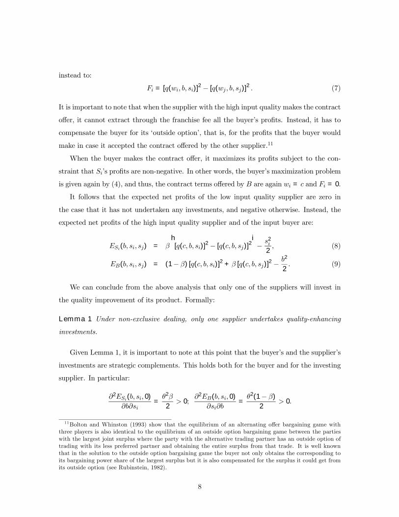
expected net profits of the high input quality supplier and of the input buyer are:

ESi(b, si, sj) = βh[q(c, b, si)]

2 − [q(c, b, sj)]2i− s

2i

2, (8)

EB(b, si, sj) = (1− β) [q(c, b, si)]2 + β [q(c, b, sj)]

2 − b2

2. (9)

We can conclude from the above analysis that only one of the suppliers will invest in

the quality improvement of its product. Formally:

Lemma 1 Under non-exclusive dealing, only one supplier undertakes quality-enhancing

investments.

Given Lemma 1, it is important to note at this point that the buyer’s and the supplier’s

investments are strategic complements. This holds both for the buyer and for the investing

supplier. In particular:

∂2ESi(b, si, 0)

∂b∂si=θ2β

2> 0;

∂2EB(b, si, 0)

∂si∂b=θ2(1− β)

2> 0.

11Bolton and Whinston (1993) show that the equilibrium of an alternating offer bargaining game withthree players is also identical to the equilibrium of an outside option bargaining game between the partieswith the largest joint surplus where the party with the alternative trading partner has an outside option oftrading with its less preferred partner and obtaining the entire surplus from that trade. It is well knownthat in the solution to the outside option bargaining game the buyer not only obtains the corresponding toits bargaining power share of the largest surplus but it is also compensated for the surplus it could get fromits outside option (see Rubinstein, 1982).

8

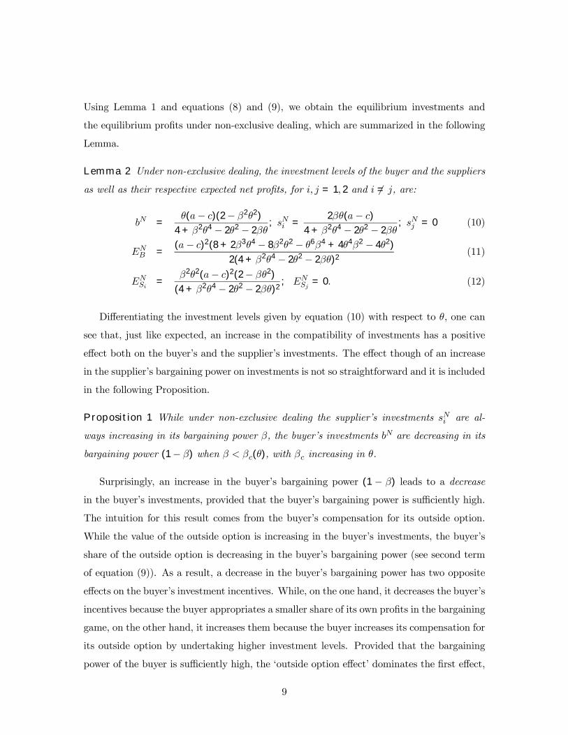
Using Lemma 1 and equations (8) and (9), we obtain the equilibrium investments and

the equilibrium profits under non-exclusive dealing, which are summarized in the following

Lemma.

Lemma 2 Under non-exclusive dealing, the investment levels of the buyer and the suppliers

as well as their respective expected net profits, for i, j = 1, 2 and i 6= j, are:

bN =θ(a− c)(2− β2θ2)

4 + β2θ4 − 2θ2 − 2βθ; sNi =

2βθ(a− c)4 + β2θ4 − 2θ2 − 2βθ

; sNj = 0 (10)

ENB =(a− c)2(8 + 2β3θ4 − 8β2θ2 − θ6β4 + 4θ4β2 − 4θ2)

2(4 + β2θ4 − 2θ2 − 2βθ)2(11)

ENSi =β2θ2(a− c)2(2− βθ2)

(4 + β2θ4 − 2θ2 − 2βθ)2; ENSj = 0. (12)

Differentiating the investment levels given by equation (10) with respect to θ, one can

see that, just like expected, an increase in the compatibility of investments has a positive

effect both on the buyer’s and the supplier’s investments. The effect though of an increase

in the supplier’s bargaining power on investments is not so straightforward and it is included

in the following Proposition.

Proposition 1 While under non-exclusive dealing the supplier’s investments sNi are al-

ways increasing in its bargaining power β, the buyer’s investments bN are decreasing in its

bargaining power (1− β) when β < βc(θ), with βc increasing in θ.

Surprisingly, an increase in the buyer’s bargaining power (1 − β) leads to a decrease

in the buyer’s investments, provided that the buyer’s bargaining power is sufficiently high.

The intuition for this result comes from the buyer’s compensation for its outside option.

While the value of the outside option is increasing in the buyer’s investments, the buyer’s

share of the outside option is decreasing in the buyer’s bargaining power (see second term

of equation (9)). As a result, a decrease in the buyer’s bargaining power has two opposite

effects on the buyer’s investment incentives. While, on the one hand, it decreases the buyer’s

incentives because the buyer appropriates a smaller share of its own profits in the bargaining

game, on the other hand, it increases them because the buyer increases its compensation for

its outside option by undertaking higher investment levels. Provided that the bargaining

power of the buyer is sufficiently high, the ‘outside option effect’ dominates the first effect,

9

and thus, a decrease in the buyer’s bargaining power has a positive impact on the buyer’s

investments.

The result regarding the supplier’s investments under non-exclusive dealing is more

intuitive. The higher is the supplier’s bargaining power, the higher is the supplier’s share

of the surplus, and thus, the higher are the supplier’s incentives to increase the surplus

through its own investments

4 Exclusive Dealing

We turn now to the analysis of the exclusive dealing case, assuming without loss of generality

that S1 is the exclusive supplier.

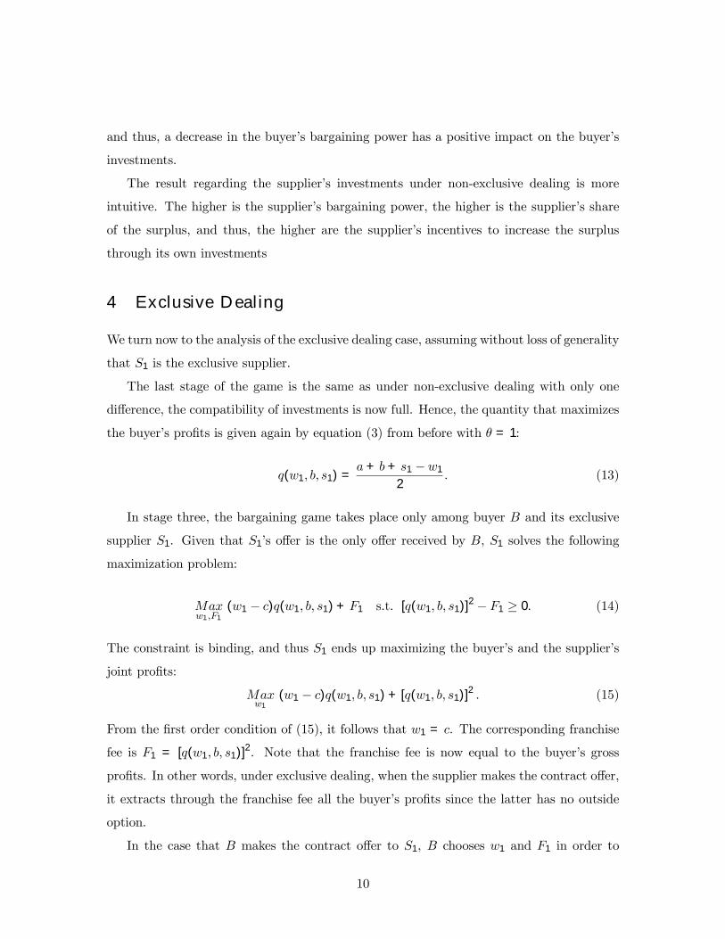
The last stage of the game is the same as under non-exclusive dealing with only one

difference, the compatibility of investments is now full. Hence, the quantity that maximizes

the buyer’s profits is given again by equation (3) from before with θ = 1:

q(w1, b, s1) =a+ b+ s1 −w1

2. (13)

In stage three, the bargaining game takes place only among buyer B and its exclusive

supplier S1. Given that S1’s offer is the only offer received by B, S1 solves the following

maximization problem:

Maxw1,F1

(w1 − c)q(w1, b, s1) + F1 s.t. [q(w1, b, s1)]2 − F1 ≥ 0. (14)

The constraint is binding, and thus S1 ends up maximizing the buyer’s and the supplier’s

joint profits:

Maxw1

(w1 − c)q(w1, b, s1) + [q(w1, b, s1)]2 . (15)

From the first order condition of (15), it follows that w1 = c. The corresponding franchise

fee is F1 = [q(w1, b, s1)]2. Note that the franchise fee is now equal to the buyer’s gross

profits. In other words, under exclusive dealing, when the supplier makes the contract offer,

it extracts through the franchise fee all the buyer’s profits since the latter has no outside

option.

In the case that B makes the contract offer to S1, B chooses w1 and F1 in order to

10

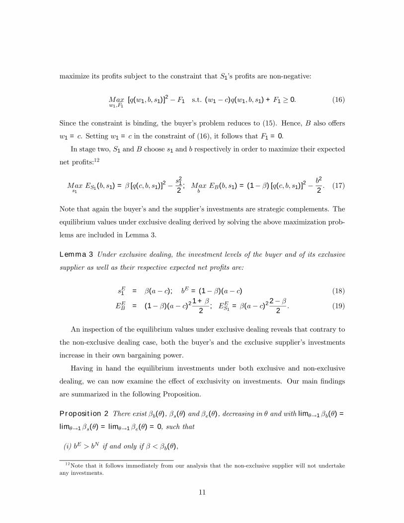
maximize its profits subject to the constraint that S1’s profits are non-negative:

Maxw1,F1

[q(w1, b, s1)]2 − F1 s.t. (w1 − c)q(w1, b, s1) + F1 ≥ 0. (16)

Since the constraint is binding, the buyer’s problem reduces to (15). Hence, B also offers

w1 = c. Setting w1 = c in the constraint of (16), it follows that F1 = 0.

In stage two, S1 and B choose s1 and b respectively in order to maximize their expected

net profits:12

Maxs1

ES1(b, s1) = β [q(c, b, s1)]2 − s21

2; Max

bEB(b, s1) = (1− β) [q(c, b, s1)]2 − b

2

2. (17)

Note that again the buyer’s and the supplier’s investments are strategic complements. The

equilibrium values under exclusive dealing derived by solving the above maximization prob-

lems are included in Lemma 3.

Lemma 3 Under exclusive dealing, the investment levels of the buyer and of its exclusive

supplier as well as their respective expected net profits are:

sE1 = β(a− c); bE = (1− β)(a− c) (18)

EEB = (1− β)(a− c)2 1 + β

2; EES1

= β(a− c)2 2− β2

. (19)

An inspection of the equilibrium values under exclusive dealing reveals that contrary to

the non-exclusive dealing case, both the buyer’s and the exclusive supplier’s investments

increase in their own bargaining power.

Having in hand the equilibrium investments under both exclusive and non-exclusive

dealing, we can now examine the effect of exclusivity on investments. Our main findings

are summarized in the following Proposition.

Proposition 2 There exist βb(θ), βs(θ) and βe(θ), decreasing in θ and with limθ→1 βb(θ) =

limθ→1 βs(θ) = limθ→1 βe(θ) = 0, such that

(i) bE > bN if and only if β < βb(θ),

12Note that it follows immediately from our analysis that the non-exclusive supplier will not undertakeany investments.

11

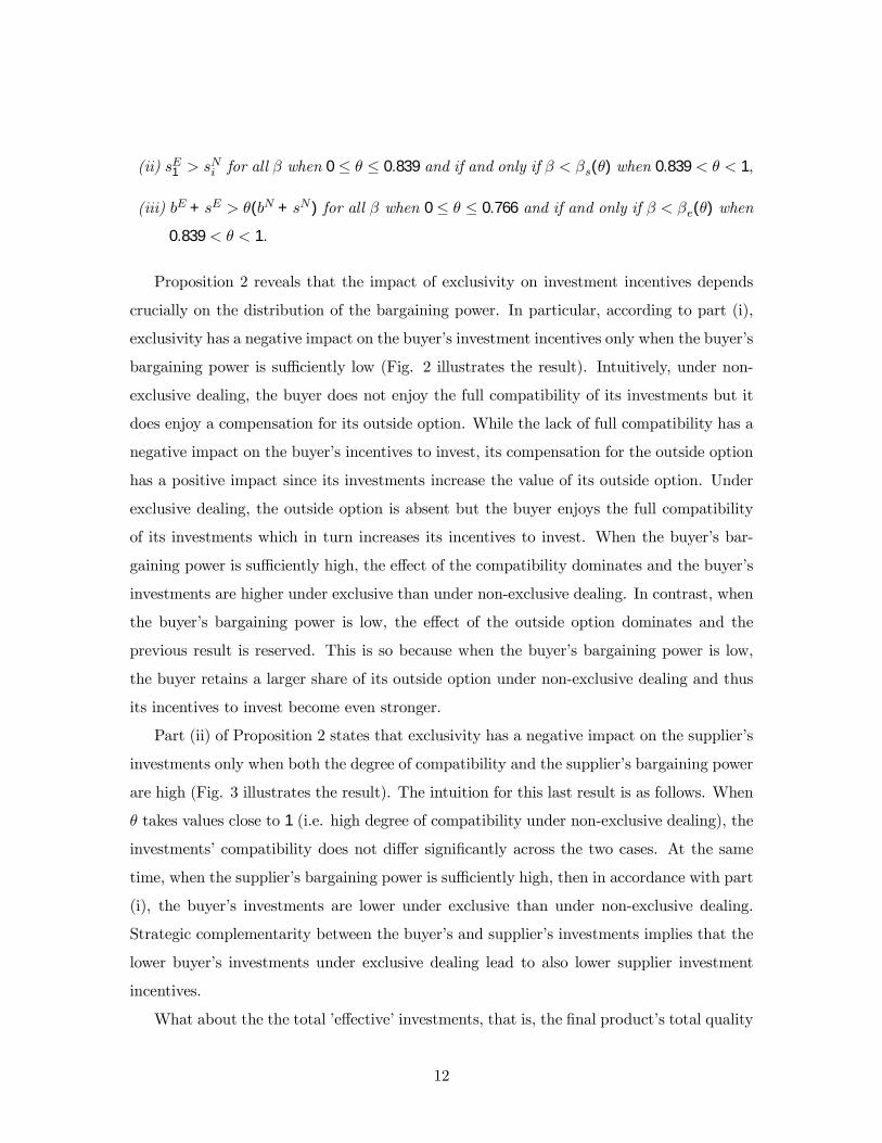
(ii) sE1 > sNi for all β when 0 ≤ θ ≤ 0.839 and if and only if β < βs(θ) when 0.839 < θ < 1,

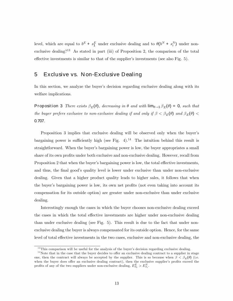
(iii) bE + sE > θ(bN + sN) for all β when 0 ≤ θ ≤ 0.766 and if and only if β < βe(θ) when

0.839 < θ < 1.

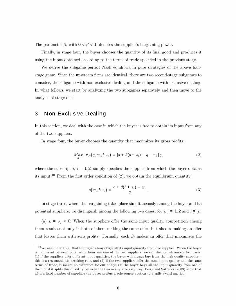
Proposition 2 reveals that the impact of exclusivity on investment incentives depends

crucially on the distribution of the bargaining power. In particular, according to part (i),

exclusivity has a negative impact on the buyer’s investment incentives only when the buyer’s

bargaining power is sufficiently low (Fig. 2 illustrates the result). Intuitively, under non-

exclusive dealing, the buyer does not enjoy the full compatibility of its investments but it

does enjoy a compensation for its outside option. While the lack of full compatibility has a

negative impact on the buyer’s incentives to invest, its compensation for the outside option

has a positive impact since its investments increase the value of its outside option. Under

exclusive dealing, the outside option is absent but the buyer enjoys the full compatibility

of its investments which in turn increases its incentives to invest. When the buyer’s bar-

gaining power is sufficiently high, the effect of the compatibility dominates and the buyer’s

investments are higher under exclusive than under non-exclusive dealing. In contrast, when

the buyer’s bargaining power is low, the effect of the outside option dominates and the

previous result is reserved. This is so because when the buyer’s bargaining power is low,

the buyer retains a larger share of its outside option under non-exclusive dealing and thus

its incentives to invest become even stronger.

Part (ii) of Proposition 2 states that exclusivity has a negative impact on the supplier’s

investments only when both the degree of compatibility and the supplier’s bargaining power

are high (Fig. 3 illustrates the result). The intuition for this last result is as follows. When

θ takes values close to 1 (i.e. high degree of compatibility under non-exclusive dealing), the

investments’ compatibility does not differ significantly across the two cases. At the same

time, when the supplier’s bargaining power is sufficiently high, then in accordance with part

(i), the buyer’s investments are lower under exclusive than under non-exclusive dealing.

Strategic complementarity between the buyer’s and supplier’s investments implies that the

lower buyer’s investments under exclusive dealing lead to also lower supplier investment

incentives.

What about the the total ’effective’ investments, that is, the final product’s total quality

12

level, which are equal to bE + sE1 under exclusive dealing and to θ(bN + sNi ) under non-

exclusive dealing?13 As stated in part (iii) of Proposition 2, the comparison of the total

effective investments is similar to that of the supplier’s investments (see also Fig. 5).

5 Exclusive vs. Non-Exclusive Dealing

In this section, we analyze the buyer’s decision regarding exclusive dealing along with its

welfare implications.

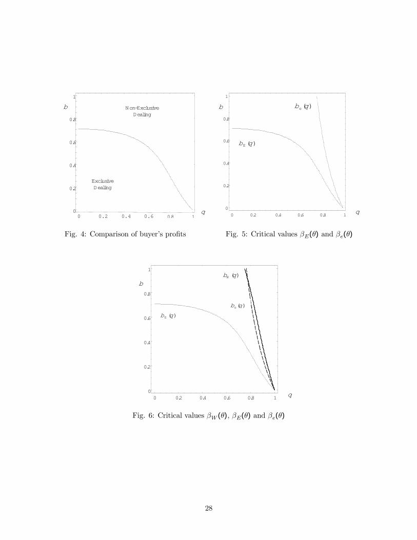
Proposition 3 There exists βE(θ), decreasing in θ and with limθ→1 βE(θ) = 0, such that

the buyer prefers exclusive to non-exclusive dealing if and only if β < βE(θ) and βE(θ) <

0.707.

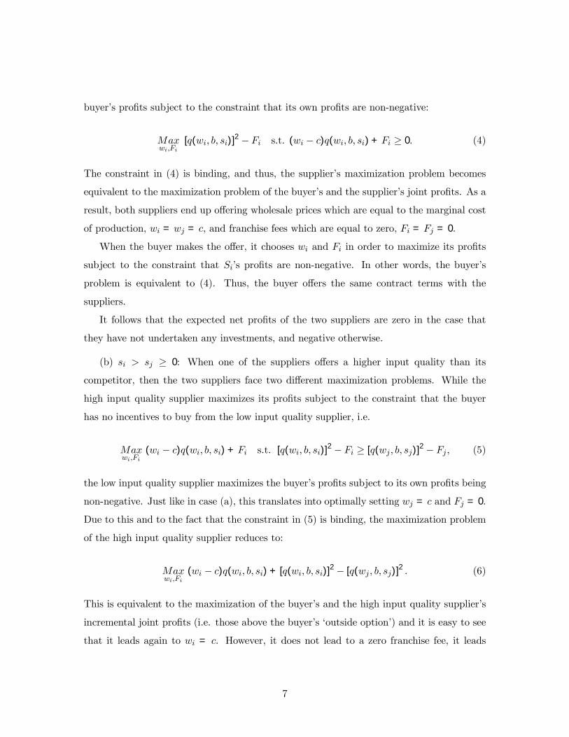
Proposition 3 implies that exclusive dealing will be observed only when the buyer’s

bargaining power is sufficiently high (see Fig. 4).14 The intuition behind this result is

straightforward. When the buyer’s bargaining power is low, the buyer appropriates a small

share of its own profits under both exclusive and non-exclusive dealing. However, recall from

Proposition 2 that when the buyer’s bargaining power is low, the total effective investments,

and thus, the final good’s quality level is lower under exclusive than under non-exclusive

dealing. Given that a higher product quality leads to higher sales, it follows that when

the buyer’s bargaining power is low, its own net profits (not even taking into account its

compensation for its outside option) are greater under non-exclusive than under exclusive

dealing.

Interestingly enough the cases in which the buyer chooses non-exclusive dealing exceed

the cases in which the total effective investments are higher under non-exclusive dealing

than under exclusive dealing (see Fig. 5). This result is due to the fact that under non-

exclusive dealing the buyer is always compensated for its outside option. Hence, for the same

level of total effective investments in the two cases, exclusive and non-exclusive dealing, the

13This comparison will be useful for the analysis of the buyer’s decision regarding exclusive dealing.14Note that in the case that the buyer decides to offer an exclusive dealing contract to a supplier in stage

one, then the contract will always be accepted by the supplier. This is so because when β < βE(θ) (i.e.when the buyer does offer an exclusive dealing contract), then the exclusive supplier’s profits exceed theprofits of any of the two suppliers under non-exclusive dealing, EE

S1> EN

Si .

13

‘effective’ bargaining power of the buyer in the case of non-exclusive dealing is higher than

that in the case of exclusive dealing.

Next, we turn to a welfare comparison of the two supply chain structures. Defining

welfare as the sum of producers’ and consumers’ surplus, we find the following.

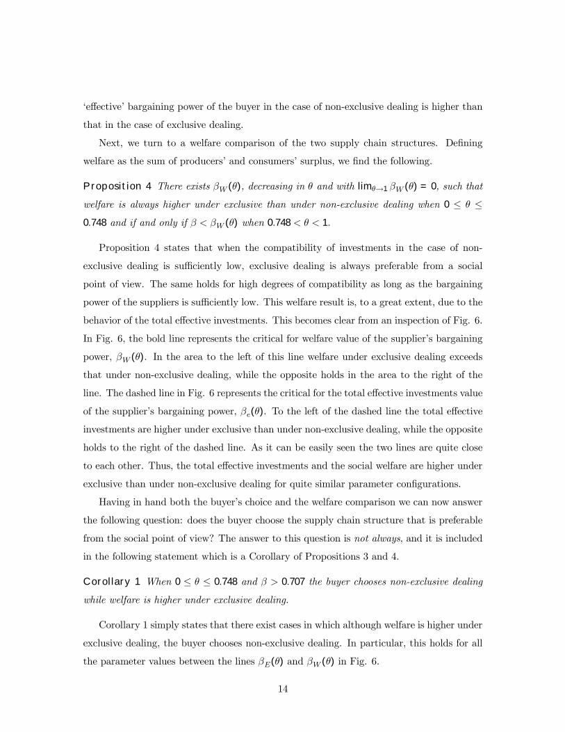
Proposition 4 There exists βW (θ), decreasing in θ and with limθ→1 βW (θ) = 0, such that

welfare is always higher under exclusive than under non-exclusive dealing when 0 ≤ θ ≤0.748 and if and only if β < βW (θ) when 0.748 < θ < 1.

Proposition 4 states that when the compatibility of investments in the case of non-

exclusive dealing is sufficiently low, exclusive dealing is always preferable from a social

point of view. The same holds for high degrees of compatibility as long as the bargaining

power of the suppliers is sufficiently low. This welfare result is, to a great extent, due to the

behavior of the total effective investments. This becomes clear from an inspection of Fig. 6.

In Fig. 6, the bold line represents the critical for welfare value of the supplier’s bargaining

power, βW (θ). In the area to the left of this line welfare under exclusive dealing exceeds

that under non-exclusive dealing, while the opposite holds in the area to the right of the

line. The dashed line in Fig. 6 represents the critical for the total effective investments value

of the supplier’s bargaining power, βe(θ). To the left of the dashed line the total effective

investments are higher under exclusive than under non-exclusive dealing, while the opposite

holds to the right of the dashed line. As it can be easily seen the two lines are quite close

to each other. Thus, the total effective investments and the social welfare are higher under

exclusive than under non-exclusive dealing for quite similar parameter configurations.

Having in hand both the buyer’s choice and the welfare comparison we can now answer

the following question: does the buyer choose the supply chain structure that is preferable

from the social point of view? The answer to this question is not always, and it is included

in the following statement which is a Corollary of Propositions 3 and 4.

Corollary 1 When 0 ≤ θ ≤ 0.748 and β > 0.707 the buyer chooses non-exclusive dealing

while welfare is higher under exclusive dealing.

Corollary 1 simply states that there exist cases in which although welfare is higher under

exclusive dealing, the buyer chooses non-exclusive dealing. In particular, this holds for all

the parameter values between the lines βE(θ) and βW (θ) in Fig. 6.

14

From an antitrust policy’s perspective, although our results indicate that the social and

the private incentives do not always coincide, they still provide an argument against the

view that exclusive dealing is an anticompetitive practice, in the case at least that exclusive

dealing is initiated by downstream producers. In fact our welfare analysis reveals that

whenever the buyer adopts exclusive dealing, welfare is also higher under exclusive dealing.

This can be seen easily in Fig. 6 where the βE(θ) line always lies to the left of the βW (θ)

line. In other words, there exist no cases in which the buyer’s choice of exclusive dealing in

equilibrium is welfare detrimental.

6 Compatibility of Investments

So far we have assumed that bθ = 1 under exclusive dealing and bθ = θ, with 0 ≤ θ < 1,

under non-exclusive dealing. In this section, we relax this assumption by considering a

model in which full compatibility is the outcome of an input supplier’s strategic choice.

The compatibility between the supplier’s and the buyer’s investments depends now on the

input supplier’s decision to open a specific research line for the buyer. In particular, if a

supplier opens a specific research line for B then the compatibility between its investments

and those of the buyer is full, bθ = 1, otherwise, bθ = θ. Since the opening of a specific line,

might be costly, we assume that in order for a supplier to achieve full compatibility with

the buyer, it has to incur a fixed cost A > 0.

We consider a similar timing with that in the basic model, modifying it only by decom-

posing stage one into two substages, stage 1(a) and stage 1(b). Stage 1(a) is exactly the

same as stage 1 of the basic model. In stage 1(b), after the choice among exclusive and

non-exclusive dealing has been made, the input suppliers S1 and S2 simultaneously and

independently decide whether or not they will open a specific line of research for B.15

Examining the supplier’s incentives to open a specific research line, we obtain the fol-

lowing result.

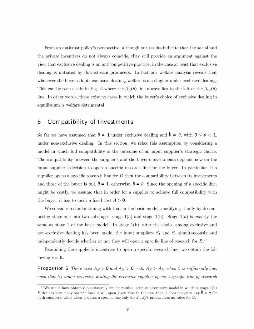
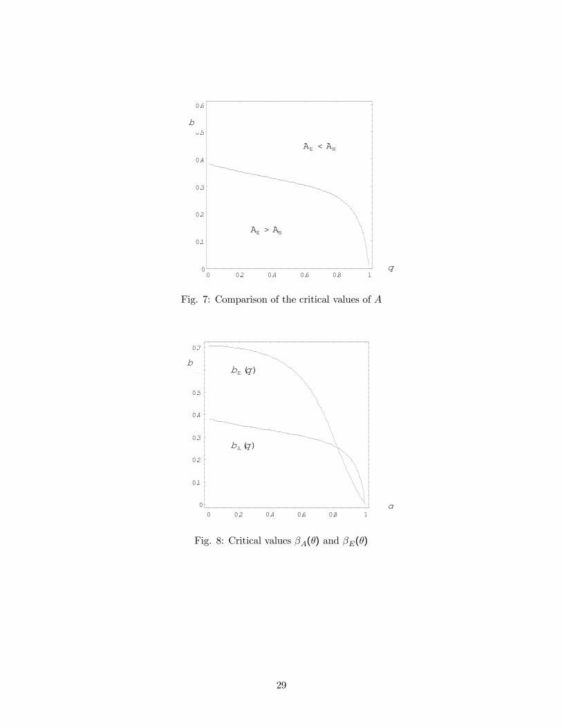
Proposition 5 There exist AE > 0 and AN > 0, with AE > AN when β is sufficiently low,

such that (i) under exclusive dealing the exclusive supplier opens a specific line of research

15We would have obtained qualitatively similar results under an alternative model in which in stage 1(b)B decides how many specific lines it will open given that in the case that it does not open any bθ = θ forboth suppliers, while when it opens a specific line only for Si, Sj ’s product has no value for B.

15

if and only if A < AE, and (ii) under non-exclusive dealing none of the suppliers opens a

specific line of research if A > AN .

Fig. 7 depicts the result included in Proposition 5. In particular, in the area under the

curve, the critical value of A below which the supplier opens a specific line under exclusive

dealing exceeds the respective critical value above which none of the suppliers opens a

specific line under non-exclusive dealing.

An important implication of Proposition 5 is that when the buyer’s bargaining power

is sufficiently high, there is a range of values of the fixed cost such that a supplier opens

a specific line for the buyer only under exclusive dealing. Clearly, the higher is the com-

patibility of investments, the higher are the investment incentives both under exclusive and

non-exclusive dealing, and thus, the larger is the surplus for the supply chain. Why then the

incentives for increasing the compatibility of investments differ across exclusive and non-

exclusive dealing? Because under non-exclusive dealing there exist two additional forces

that are absent under exclusive dealing. The first force is the previously mentioned ‘outside

option effect’ which leads to higher investment incentives. The second force is related to

the fact that under non-exclusive dealing the supplier has to compensate the buyer for its

outside option. The higher is the compatibility of investments, the higher are the buyer’s

investments, and thus, the higher is the value of the outside option that the supplier has

to compensate the buyer for. Obviously, while the first force, the ‘outside option effect’,

strengthens the supplier’s incentives to open a specific line under non-exclusive dealing,

the second force weakens them. Now why is the ‘outside option effect’ dominated when

the buyer’s bargaining power is sufficiently high (i.e. when β is low enough)? This is so

because, as mentioned in the intuition of Proposition 2, when the buyer’s bargaining power

is sufficiently high, the ‘outside option effect’ is weaker.

Corollary 2 simply summarizes the above implication.

Corollary 2 If AN < A < AE, then bθ = 1 under exclusive dealing and bθ = θ under

non-exclusive dealing.

In other words, there exists a range of values of the cost of opening a specific research

line, such that our basic model with its compatibility assumption can be justified as a

reduced form of the more general model analyzed here. It follows that in this range our

16

previous analysis applies.

Finally, it is important to examine whether the cases that the buyer chooses exclusive

dealing in the basic model, correspond to the cases that compatibility can be full only under

exclusive dealing in the extended model. In particular, we know from the basic model that

the buyer opts for exclusive dealing when its bargaining power is sufficiently high, that is,

in the area below the βE(θ) curve in Fig. 8. In addition, we know from the extended

model that compatibility could, under some circumstances, turn out to be full only under

exclusivity in the area below the βA(θ) curve in Fig. 8. It follows that exclusive dealing

with full compatibility could emerge in equilibrium in the intersection of the areas, provided

however that the costs of a specific research line take some intermediate value.

7 Conclusion

We have studied the incentives of final product manufacturers to develop exclusive rela-

tions with their input suppliers taking into account the fact that such relations are usually

characterized by high buyer-supplier coordination.

Contrary to the existing literature on buyer-initiated exclusive dealing (see e.g., Se-

gal and Whinston, 2000), which has not considered the high compatibility of buyer’s and

supplier’s investments under exclusive relations, we have showed that an input buyer’s in-

centives for exclusive dealing depend crucially on the distribution of bargaining power. In

particular, we have showed that the buyer opts for exclusive dealing only when its bargain-

ing power is sufficiently high. This finding clearly suggests that the observed existence of

both exclusive and non-exclusive supply chain structures could be also due to differences in

the final product manufacturers’ bargaining positions relative to their input suppliers.

Interestingly enough we have found that there exist cases in which although investments

are higher under exclusive dealing, the buyer chooses non-exclusive dealing. This occurs

because the buyer’s decision is affected by the fact that competition among the suppliers

is present only under non-exclusive dealing. This, of course, allows us to put forward the

point that investments are not the only force at work in the buyer’s decision whether or not

it will adopt exclusive dealing.

From a policy perspective, we have found that the buyer’s choice of exclusive dealing

17

in equilibrium is never harmful to welfare. Hence, our results provide an argument against

the view that exclusive dealing is an anticompetitive practice, in the cases at least that

exclusive dealing is initiated by downstream final product manufacturers.

In sum, we have provided a simple theoretical foundation for the frequently observed

buyer-initiated exclusive relations in supply chains. Our paper is just a first step towards

this direction. In future work we plan to extend our analysis by considering unobservable

degrees of compatibility as well as by examining the strategic incentives for exclusive dealing

in a setting with downstream competition.16

8 Appendix

Proof of Lemma 1: Case (a), with si = sj ≥ 0, cannot be an equilibrium because one of

the suppliers will always have incentives to deviate. In particular, when si = sj = 0 both

suppliers have zero profits and one of them always has incentives to deviate and undertake

positive investments because by doing so it will earn positive profits. Similarly, when

si = sj > 0 both suppliers make negative profits and one of them always has incentives to

deviate by not undertaking any investments so that its profits are equal to zero. Given that

one of the suppliers will undertake higher investments than the other and thus that it will

offer a higher quality input, we can conclude that the supplier with the lower quality input

will undertake zero investments because otherwise, it will make negative profits. Q.E.D.

Proof of Lemma 2: We know from Lemma 1 that the equilibrium will take the following

form: (b, si, sj) = (bN , sNi , 0), with i, j = 1, 2, i 6= j and sNi > 0. W.l.o.g. we assume that

S1 is the supplier that undertakes positive investments. In order to find the equilibrium

levels of b and s1 we proceed in the following way. We start by assuming that S2 deviates

and chooses s2 > s1. If s2 > s1, then in accordance with case (b), in stage three, w2 = c

and

F2 =[a+ θ(b+ s2)− c]2

4− [a+ θ(b+ s1)− c]2

4(20)

16Fumagalli and Motta (2004) use a setting with downstream competition in order to analyze the effectof supplier-initiated exclusive dealing on entry.

18

with probability β. The respective expected profits of the deviating supplier are:

ES2(b, s1, s2) = β

·[a+ θ(b+ s2)− c]2

4− [a+ θ(b+ s1)− c]2

4

¸− s

22

2(21)

From the first order condition of (21) w.r.t. s2, it follows that S2’s profits in case of deviation

are maximized when it chooses the following level of investments:

s∗2 = βθa− c+ θb

2− βθ2 (22)

In order for S2 not to have incentives to deviate, it is sufficient that s1 ≥ s∗2. This is

so because when s1 ≥ s∗2, the deviation profits of S2 are negative. The last thing for

determining the equilibrium in stage two is to find the investment levels that S1 and B

choose in order each to maximize their profits under the constraint that s1 ≥ s∗2.Formally,S1 and B solve the following maximization problems:

Maxs1

ES1(b, s1, s2) = β

·[a+ θ(b+ s1)− c]2

4− [a+ θb− c]2

4

¸− s

21

2s.t. s1 ≥ s∗2

Maxb

EB(b, s1, s2) = (1− β)[a+ θ(b+ s1)− c]2

4+ β

[a+ θb− c]24

− b2

2.

From the first order conditions of the two maximization problems, we have:

s1(b) = βθa− c+ θb

2− βθ2 ; b(s1) = θa− c+ θ(1− β)s1

2− θ2 (23)

Solving the above system of equations, we obtain the investment levels of B and S1 given by

equation (10). It is easy to check that these are the equilibrium investment levels, since the

value of s1given by equation (10) does satisfy the constraint s1 ≥ s∗2. Finally, substituting(10) in the expected net profits of B and S1 we obtain their equilibrium profits under

non-exclusive dealing, given by equations (11) and (12) respectively. Q.E.D.

Proof of Proposition 1: We differentiate the equilibrium values given by equation (10)

with respect to β and our result follows immediately. Q.E.D.

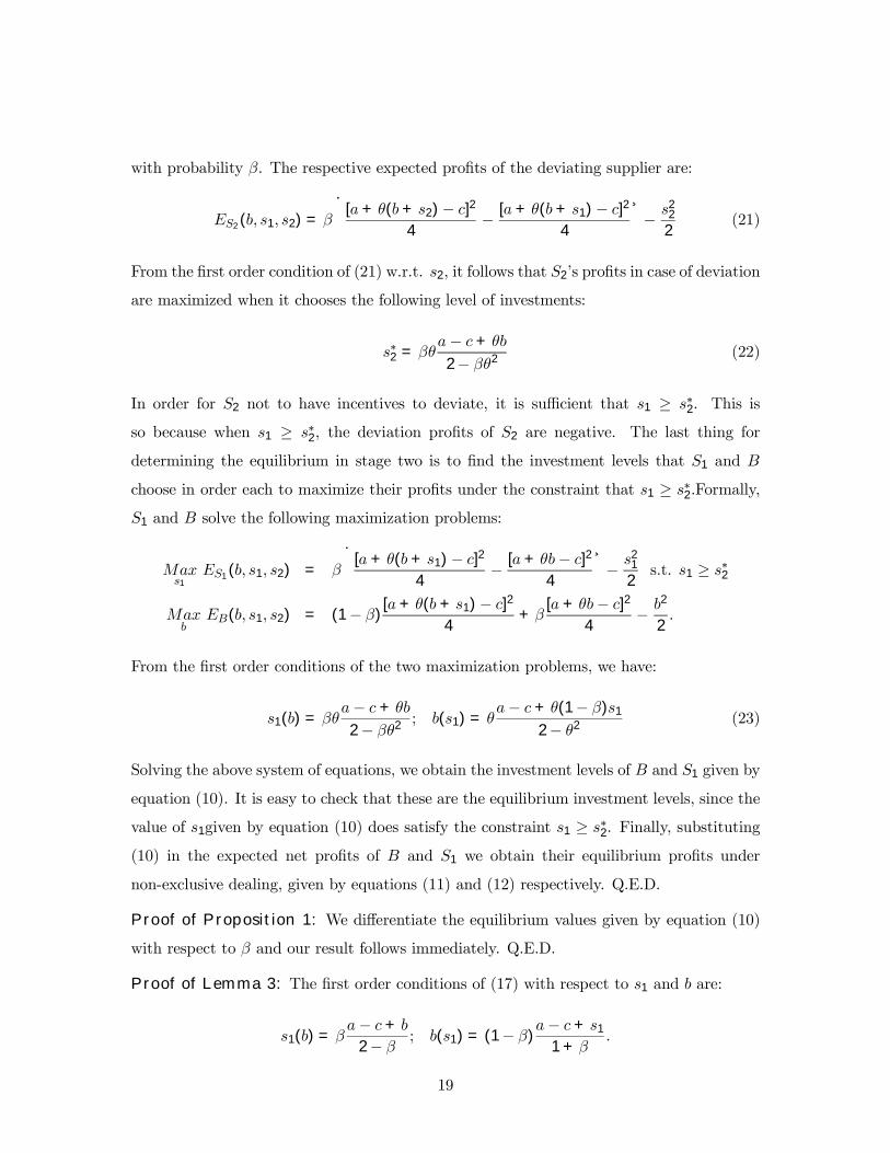
Proof of Lemma 3: The first order conditions of (17) with respect to s1 and b are:

s1(b) = βa− c+ b

2− β ; b(s1) = (1− β)a− c+ s1

1 + β.

19

Solving the above system of equations, we obtain the equilibrium levels of investments given

by (18). Finally, substituting these equilibrium values into the profit functions of S1 and

B, we obtain their equilibrium expected net profits included in equation (19). Q.E.D.

Proof of Proposition 2: (i) Taking the difference of equations (18) and (10), we have:

bE − bN =(a− c)Nb

D= K1,

where D = 4 + β2θ4 − 2θ2(1 + β) and Nb = 4 − 4β − 2θ − 2θ2 + β2θ2(2 + θ2 − βθ2 + θ).

The denominator, D, is always positive. Setting the numerator, equal to zero and solving

for the critical value of β in terms of θ, we obtain:

βb(θ) =1

3θ2

"2 + θ2 + θ − 3

qR+ 3

√W − 5θ2 + 4θ + θ4 + 2θ3 − 8

3pR+ 3

√W

#> 0

where R = 28 + 6θ − 54θ2 + 14θ3 + 18θ4 − θ6 − 3θ5 and W = 144− 48θ − 396θ2 + 72θ3 +

516θ4 − 132θ5 − 213θ6 + 21θ8 + 66θ7 − 6θ10 − 24θ9. Next we calculate K1 at the extreme

values of β:

limβ→0

K1 =(a− c)(2 + θ)(1 + θ)

2− θ2 > 0 and limβ→1

K1 =(a− c)θθ2 − 2

< 0.

It follows from the above that K1 > 0 iff β < βb(θ). Moreover, differentiating K1 w.r.t. θ

we find that ∂K1/∂θ < 0. Thus, we also have that ∂βb(θ)/∂θ for all values of θ. Finally,

in order to show that limθ→1 βb(θ) = 0, we calculate the limθ→1(bN/bE). It can be checked

that the latter is strictly increasing in β and that it is equal to zero for β = 0.

(ii) Taking the difference of equations (18) and (9), we have:

sE1 − sNi =(a− c)Ns

D= K2,

where Ns = 4−2βθ2−2θ2 +β2θ4−2θ. The denominator, D, is always positive. Regarding

the numerator, differentiating it w.r.t. β we have: ∂Ns/∂β = 2θ2(βθ2 − 1) < 0. Thus, it

takes its maximum value when β → 0 and its minimum value when β → 1. In particular:

limβ→0Ns = 2(1 + θ)(2 + θ) > 0 and limβ→1Ns = (θ − 2)(θ3 + 2θ2 − 2). Setting the latter

20

equal to zero and solving for θ, we have:

θ =1

3

"3

q19 + 3

√33 +

43p

19 + 3√

33− 2

#' 0.839.

Since limβ→1Ns > 0 iff 0 ≤ θ ≤ 0.839, it follows that Ns > 0 when 0 ≤ θ ≤ 0.839 for all

the values of β. Setting Ns = 0 and solving for the critical value of β, we have:

βs(θ) =1−

p2θ + 2θ2 − 3

θ2 .

Since we know from the above that when 0.839 < θ < 1, limβ→0Ns > 0 and limβ→1Ns < 0,

it follows that when 0.839 < θ < 1, Ns > 0 iff β < βs(θ). Moreover, we find that

∂βs(θ)/∂θ < 0. It follows from this that βs(θ) takes its minimum value when θ → 1.

Since limθ→1 βs(θ) = 0, it follows that βs(θ) > 0 when 0.839 < θ < 1.

(iii) Taking the difference of the effective total investments, we have:

bE + sE1 − θ(bN + sNi ) = (a− c)NeD

= (a− c)K3, (24)

where Ne = 2(2−2βθ2−2θ2 +β2θ4). Differentiating K3 w.r.t. θ, we find that ∂K3/∂θ < 0.

Moreover we have that while limβ→0K3 > 0 holds always, limβ→1K3 > 0 holds iff 0 ≤ θ ≤0.766. Thus, when 0 ≤ θ ≤ 0.766, then K3 > 0. Setting K3 = 0 and solving for the critical

value of β in terms of θ, we have:

βe(θ) =1−

q(−1 + 2θ2)

θ2 .

Since we know from above that when 0.766 < θ < 1, limβ→0K3 > 0 and limβ→1K3 > 0,

it follows that when 0.766 < θ < 1, then K3 > 0 iff β < βe(θ). Moreover, we find that

limθ→1 βe(θ) = 0 and that for 0.766 < θ < 1, we have ∂βe(θ)/θ < 0. Q.E.D.

Proof of Proposition 3: Taking the difference of equations (19) and (10), we have the

following:

EEB −ENB =(a− c)2NE

2D2= (a− c)2K4,

where NE = 8 + 4β2θ4 − 16βθ2 + 8βθ4 − 4β3θ6 − 12θ2 + 4θ4 − 4θ6β2 + β4θ8 − 12β4θ4 +

21

16β3θ2−10β3θ4 +4β5θ6−16β2 +24β2θ2 +5θ6β4−β6θ8. Differentiating K4 w.r.t. θ we find

that ∂K4/∂θ < 0. Moreover we find that while limθ→1K4 < 0 holds always, limθ→0K4 < 0

holds iff β > 1/√

2 ' 0.707. Thus, when β > 0.707, we have K4 > 0. It is easy to show that

∂K4/∂β < 0 when 0 < β < 0.707, as well as that limβ→0.707K4 < 0 and limβ→0K4 > 0.

It follows then that when 0 < β < 0.707, there exists βE(θ) > 0 such that K4 > 0 iff

β < βE(θ). Since ∂K4/∂θ < 0, we also have that ∂βE(θ)/∂θ < 0. Finally, in order to show

that limθ→1 βE(θ) = 0, we calculate the limθ→1(ENB /EeB). It can be checked that the latter

is strictly increasing in β and that it is equal to zero for β = 0. Q.E.D.

Proof of Proposition 4: Calculating welfare both under exclusive dealing and under

non-exclusive dealing, we have:

WE = (a− c)2(1 + β − β2) and WN = (a− c)2 12− 4θ2 − 4θ2β2 + 4θ4β2 − θ6β4

2(4− 2θ2 − 2βθ2 + β2θ4)2.

Their difference is given by:

WE −WN = (a− c)2NWDW

= (a− c)2K5,

where DW = 2[4−2θ2(1+β)+β2θ4]2 > 0 and NW = 2(1+β−β2)[4−2θ2(1+β)+β2θ4]2−12 + 4θ2(1 + β2) − 4β2θ4 + β4θ6. It is easy to check that K5 > 0 when 0 ≤ θ ≤ 0.748 for

all β, and that limθ→1K5 < 0 and limθ→0K5 < 0. In order to define the critical value of

β, for 0.748 < θ < 1, we set NW = 0. Taking the total derivative of NW = 0, we have

dβ/dθ = −(∂NW/∂θ)/(∂NW/∂β), substituting NW = 0 in the latter, one can check that

it is always negative. It follows that when 0.748 < θ < 1, there exists βW (θ) > 0 such

that K5 > 0 iff β > βW (θ) with βW (θ) strictly decreasing in θ. In order to show that

limθ→1 βW (θ) = 0, we calculate the limθ→1(WN/WE). It can be checked that the latter is

strictly increasing in β and equal to zero for β = 0. Q.E.D.

Proof of Proposition 5: (i) In the case of exclusive dealing, when S1 opens in stage 1(b)

a specific line for B, the continuation of the game is exactly the same as the one included

in section 4. Thus, the profits of S1 are given by the difference of equation (19) and the

fixed cost A. We denote this profits with EEAS1. When S1 does not open a specific line for

B in stage 1(b), we follow exactly the same procedure as the one included in section 4 with

22

the only difference that we no longer assume that bθ = 1. Doing so, we obtain the profits of

S1 when it does not open the specific line:

EENS1= β(a− c)2 2− θ2β

2(2− θ2)2.

Taking the difference of the profits, setting it equal to zero, EEAS1−EENS1

, and solving for A,

we find:

AE = β(a− c)2(1− θ2)6− 4β + θ2β − 2θ2

2(2− θ2)2.

Since the EENS1profits are always lower than that given by equation (19), it follows that S1

opens a specific line of research for B, when A < AE .

(ii) In the case of non-exclusive dealing when none of the suppliers opens a specific

line, the analysis is exactly the same as the one included in section 3. Thus, the profits

of Sj are zero while those of Si are positive and are given by equation (12). In order for

this to be the equilibrium, that is, in order none of the suppliers to open a specific line it

is sufficient to show that Sj does not have incentives to deviate and open a specific line.

W.l.o.g. we assume for the rest of the proof, that in the case where none of the suppliers

opens a specific line, S2 is the supplier with the zero profits and S1 is the supplier with the

positive profits. In case that S2 deviates and incurs A, then the continuation of the game

is similar to that in section 3. The only difference is that the degree of compatibility is now

asymmetric for the two suppliers, that is, bθ = 1 for the investments of S2, and bθ = θ with

0 ≤ θ < 1, for the investments of S1. Next we provide the continuation of the game in the

case of deviation. In stage four, B chooses its output in order to maximize its gross profits:

πB = [a+ bθ(b+ si)− q −wi]q. The equilibrium quantity of the final good is:

q(wi, b, si) =a+ bθ(b+ si)−wi

2,

where the subscript i = 1, 2 indicates the supplier from which B obtains the input. In case

it obtains the input from S2, bθ = 1, while in the case it obtains it from S1, bθ = θ. In stage

three, we distinguish among the following three cases:

(a) b+ s2 = θ(b+ s1): Similarly to the case with symmetric bθ we have (wi, Fi) = (c, 0).

(b) b+s2 > θ(b+s1): In this case w1 = w2 = c for both suppliers, however while F1 = 0,

23

F2 with probability β is equal to:

F2 =(a+ b+ s2 − c)2

4− (a+ θ(b+ s1)− c)2

4,

and with the rest of the probability is equal to zero.

(c) b+s2 < θ(b+s1): In this case w1 = w2 = c for both suppliers, however while F2 = 0,

F1 is with probability 1− β equal to zero and with probability β equal to:

F1 =[a+ θ(b+ s1)− c]2

4− (a+ b+ s2 − c)2

4.

It follows from the above that Lemma 1 holds here too. Next, we analyze the case in

which S2 is the supplier that undertakes the positive investment levels. Later on we will

show that indeed in equilibrium S2 and not S1 will be the supplier that undertakes the

positive investment levels. In order to find the equilibrium levels of b and s2 we proceed

in the following way. We start by assuming that S1 deviates and chooses s1 such that

b+ s2 < θ(b+ s1), that is, s1 > [s2 + b(1− θ)]/θ and then we follow the same procedure asthe one in the proof of Lemma 2. Doing so, we find the following investment levels:

sNA2 =(a− c)β(2 + βθ − βθ2)

2− 2βθ2 + β2θ2 and bNA =(a− c)(2 + 2βθ − 2β − β2θ)

2− 2βθ2 + β2θ2 .

The respective expected net profits of supplier S2 are:

ENAS2=

β(a− c)2NA

2− 2βθ2 + β2θ2 −A,

whereNA = 6−β3θ4+2β3θ3−4β2θ−β3θ2+4β2θ2+12βθ−4β2θ3−4βθ2−4β+2β2θ4−2θ2−4θ.

Setting ENAS2= 0 and solving for A, we find:

AN =β(a− c)2N2

2(2− 2βθ2 + β2θ2)2.

It follows that S2 does not open a specific line of research for B, when A > AN .

Finally, setting AE −AN = 0, we can implicitly define βA(θ). Since it is impossible to

get an analytical expression for βA(θ), in order to show that AE > AN , we need to evaluate

24

instead the following limit:

limβ→0

AEAn

=4(3− θ2)(1 + θ)

(3 + θ)(θ2 − 2)2> 1.

It follows from the above that for sufficiently small β, we have that AE > AN . Q.E.D.

9 References

Besanko, D. and M. Perry (1993), “Equilibrium Incentives for Exclusive Dealing in a

Differentiated Products Oligopoly,” RAND Journal of Economics, 24, 646-667.

Bernheim, B. and M. D. Whinston (1998), “Exclusive Dealing,” Journal of Political Econ-

omy, 106, 64-103.

Bolton, P. and M. D. Whinston (1993), “Incomplete Contracts, Vertical Integration, and

Supply Assurance,” Review of Economic Studies, 60, 121-148.

Che, Y.-K. and J. Sákovics (2004), “Contractual Remedies to the Holdup Problem: A

Dynamic Perspective,” unpublished manuscript, University of Edinburgh.

Chemla, G. (2003), “Downstream Competition, Foreclosure and Vertical Integration,”

Journal of Economics and Management Strategy, 12, 261-289.

Cusumano, A. and A. Takeishi (1991), “Supplier Relations and Management: A Survey of

Japanese, Japanese-Transplant, and U.S. Auto Plants,” Strategic Management Jour-

nal, 12, 563-588.

De Fraja, G. and J. Sákovics (2001), “Walras Retrouvé: Decentralized Trading Mechanisms

and the Competitive Price,” Journal of Political Economy, 109, 842-863.

De Meza, D. and M. Selvaggi (2003), “Please Hold Me Up: Why Firms Grant Exclusive

Dealing Contracts,” CMPO Working Paper Series 03/066.

Fumagalli, C. and M. Motta (2004), “Exclusive Dealing and Entry When Buyers Com-

pete,” unpublished manuscript, European University Institute.

25

Grossman, S. J. and O. Hart (1986), “The Costs and Benefits of Ownership: A Theory of

Vertical and Lateral Integration,” Journal of Political Economy, 94, 691-719.

Hart, O. and J. Moore (1988), “Incomplete Contracts and Renegotiation,” Econometrica,

56, 755-785.

Helper, S. (1991), “How Much Has Really Changed Between U.S. Automakers and Their

Suppliers?” Sloan Management Review, 32, 15-28.

Helper, S. and M. Sako (1995), “Supplier Relations in Japan and the United States: Are

They Converging?” Sloan Management Review, 36, 77-84.

Klein, B. (1988), “Vertical Integration as Organizational Ownership: The Fisher Body-

General Motors Relationship Revisited,” Journal of Law, Economics and Organiza-

tion, 4, 199-213.

Klein, B., R. G. Crawford and A. A. Alchian (1978), “Vertical Integration, Appropriable

Rents, and the Competitive Contracting Process,” Journal of Law and Economics,

21, 297-326.

Marvel, H. P. (1982), “Exclusive Dealing,” Journal of Law and Economics, 25, 1-25.

Moore, N., L. Baldwin, F. Camm and C. Cook (2002), Implementing Best Purchasing and

Supply Management Practices: Lessons From Innovative Commercial Firms, Santa

Monica: Rand Publications.

Perry, M. and J. Sákovics (2003), “Auctions for Split-Award Contracts,” Journal of In-

dustrial Economics, 51, 215-242.

Rey, P. and J. Tirole (2003), “A Primer on Foreclosure,” in Handbook of Industrial Orga-

nization, Vol. 3, Elsevier, North Holland, Amsterdam, forthcoming.

Rubinstein, A. (1982), “Perfect Equilibrium in a Bargaining Model,” Econometrica, 50,

97-109.

Segal, I. and M. D. Whinston (2000), “Exclusive Contracts and Protection of Investments,”

RAND Journal of Economics, 31, 603-633.

26

Tirole, J. (1986), “Procurement and Renegotiation,” Journal of Political Economy, 94,

235-259.

Williamson, O. (1985), The Economic Institutions of Capitalism, New York: Free Press.

• •2 4

B decides Exclusivityor Non-Exclusivity

Investmentsof B , S 1 and S2

Bargainingover (wi, Fi)

1 3

Final Good Production

Fig. 1: Stages of the game

0 0.2 0.4 0.6 0.8 1

0

0.2

0.4

0.6

0.8

1

0 0.2 0.4 0.6 0.8 10

0.2

0.4

0.6

0.8

1

Ni

E ss >1

b

q

bE > bN

bE < bN

q

b

Fig. 2: Comparison of B’s investments Fig. 3: Comparison of Si’s investments

27

0 0.2 0.4 0.6 0.8 10

0.2

0.4

0.6

0.8

1

0 0.2 0.4 0.6 0.8 1

0

0.2

0.4

0.6

0.8

1

q

b

ExclusiveDealing

Non-Exclusive Dealing

q

b

)(qbE

)(qbe

Fig. 4: Comparison of buyer’s profits Fig. 5: Critical values βE(θ) and βe(θ)

0 0.2 0.4 0.6 0.8 10

0.2

0.4

0.6

0.8

1

)(qbe

)(qbE

)(qbW

q

b

Fig. 6: Critical values βW (θ), βE(θ) and βe(θ)

28

0 0.2 0.4 0.6 0.8 10

0.1

0.2

0.3

0.4

0.5

0.6

NE AA <

NE AA >

q

b

Fig. 7: Comparison of the critical values of A

0 0.2 0.4 0.6 0.8 1

0

0.1

0.2

0.3

0.4

0.5

0.6

0.7

q

b )(qbE

)(qbA

Fig. 8: Critical values βA(θ) and βE(θ)

29