documentos de economÍa y finanzas internacionales …aeefi.com/repec/pdf/defi18-01.pdf · 1...
TRANSCRIPT

1
DOCUMENTOS DE ECONOMÍA YFINANZAS INTERNACIONALES
Working Papers on InternationalEconomics and Finance
DEFI 18-01Julio 2018
Time-varying cointegrating regression analysis with anapplication to the long-run interest rate pass-through in the
Euro AreaAfonso-Rodríguez, Julio A. Santana-Gallego, María
Asociación Española de Economía y Finanzas Internacionaleswww.aeefi.comISSN: 1696-6376

Time-varying cointegrating regression analysis
with an application to the long-run interest rate
pass-through in the Euro Area
Afonso-Rodríguez, Julio A. Department of Applied Economics and Quantitative Methods
University of La Laguna
Camino La Hornera, s/n. Campus de Guajara, C.P. 38071 La Laguna, Tenerife, Canary Islands
Teléfono: 922317041, e-mail: [email protected]
Santana-Gallego, María Department of Applied Economics
University of the Balearic Islands
Edificio Gaspar Melchor de Jovellanos, Campus UIB
Cra. Valldemossa, km 7.5, C.P. 07122 Palma (Illes Balears)
Teléfono: 971171383, e-mail: [email protected]
Abstract
This paper study the mechanism of transmission between the money and the retail credit
markets stated in terms of the long-run relationship between the harmonized interest
rates for different credit categories and for a subset of countries of the EMU (European
Monetary Union). This mechanism, known as the interest rate pass-through (IRPT)
phenomenon, has been analyzed in many empirical studies using a variety of econometric
techniques, for different samples of countries and periods of time, and the general
conclusion is that the pass-through seems to be incomplete in the long-run. Except for a
few recent works, the analysis is performed on the basis on a time-invariant long-run
relationship which may not be appropriate in this case and could condition this result. To
evaluate the robustness of these findings we extend the analysis through a non-linear
model for the long-run relationship between the money and the retail markets that
incorporates in a very flexible form, and with minimum requirements on tuning
parameters, the nonlinearity in the form of time-varying parameters. To that end we
follow the approach initiated in Bierens (1997) and also propose some new tools to test
for the existence of a stable time-varying cointegration relationship. The results obtained
seems to support the former evidence of an incomplete pass-through.
Keywords and phrases: retail interest rates, monetary policy, cointegration
analysis, structural instability, time-varying cointegration
JEL classification: E52, F36, C22

1
1. Introduction
Monetary transmission is a key issue when analyzing monetary policy decisions. In
this sense, the transmission of monetary policy relies on how policy rate changes,
measured as changes in money market interest rates, are transferred to the bank
system via changes in the retail rates for each possible credit category in the
economy, which is called the interest rate pass-through (IRPT) effect. This
mechanism is important for achieving the aims of monetary policy, such as
achieving price stability and influencing the path of the real economy through
influencing aggregate demand at least to some extent. This phenomenon is closely
related to the analysis of the stability properties of monetary policy rules in terms
of giving rise to a unique and stable equilibrium if the implied response of the
nominal interest rates to inflation changes is sufficiently strong (Taylor principle).
An incomplete IRPT could violate the Taylor principle and monetary policy would
fail to be stabilizing in the sense that retail interest rates do not respond
sufficiently to ensure that real rates are stabilizing. This appears to be particularly
important for the Euro Area, usually taken as an example of a bank-based financial
system, for which the empirical evidence seems to indicate a limited IRPT (retail
interest rates responding less than one-to-one to policy rates).1
This paper contributes to the empirical analysis of measuring the magnitude of the
adjustment in the framework of analysis of a non-linear model for long-run
relationship allowing for a time-varying relationship between the money market
and the retail interest rates for a set of EMU countries selected by the criterion of
having the longest available series.
The structure of the paper is as follows: Section 2 briefly reviews the motivation
and relevance of IRPT and some empirical findings in this literature, while that in
section 3 we contribute to the analysis of the specification of a general time-
varying cointegrating model, both in the form of a time-varying cointegrating
regression model or, alternatively, as a reduced rank time-varying error-correction
model (ECM), and discuss some of their main features. Section 4 introduce the
empirical analysis based on evaluating the existence of a time-varying
cointegration relationship between the selected interest rate series, adopting the
methodology introduced in Bierens (1997) that propose to model the parameters
as smooth functions of time through a weighted average of Chebyshev time
polynomials. This methodology has been used before in Bierens and Martins
(2010) and in Neto (2012, 2014), but we propose some new tools to empirically
assess the stability of the non-linear relationship allowing for consistent estimates
of the instantaneous and time-varying magnitudes of the IRPT. Finally, some
theoretical developments are presented in Appendixes A to C, while the main
empirical results are presented in Appendixes D to F.
2. Monetary transmission pass-through
Since the origin of the Economic and Monetary Union in Europe (EMU), a large
number of empirical studies have tried to find evidence of possible differences in
the impact of monetary policy changes on output and inflation rates among
1 See, e.g., Kwapil and Scharler (2010) and the references cited on earlier empirical studies for EMU
countries and different periods of time.

2
European countries. Also, given that the mechanism of setting policy rates can be
viewed as the standard tool of monetary policy, the implementation of the
monetary policy through open market operations tries to ensure that policy rates
are transmitted to the interest rates at which financial institutions refinance. The
characteristics of the process of transmission of monetary policy rules, from
changes in the policy rates to retail bank rates, has consequences on the stability
properties of some theoretical models incorporating short and long-run
relationship between monetary policy targets on interest rate on bonds and
(expected) inflation rates and output (see, e.g., Kwapil and Scharler (2010), and
Kobayashi (2008)).
At the retail level, many of such studies have been conducted in an attempt to
estimate the degree of interest rate pass-through (IRPT) in the EMU system. In this
literature, the term IRPT generally has two meanings: loan rate pass-through and
deposit rate pass-through. Bank decisions regarding the paids on their assets and
liabilities have an impact on the expenditure and investment behaviour of deposit
holders and borrowers and thus on real economy activity. However, the channel of
transmission of policy rates to lending and deposit rates (IRPT) can suffer from
some types of failures given that it is affected by various factors, as could be the
case in periods of low economy activity where financial intermediaries may
require higher compensations for risk and hence changes in the policy rate would
only partially be passed on to firms or households. Also, the time and degree of
pass-through of official and market interest rates to retail bank interest rates
condition the effectiveness of monetary policy transmission and thus may affect
price stability. Furthermore, price set by banks influence their margins and
profitability and hence the solvency of the banking system and thus financial
stability. However, on the basis of formal theoretical models of monetary
transmission mechanisms with sticky prices and the evidence of loan rate
stickiness in the short run, i.e., changes in short-term market interest rates are not
immediately fully reflected in retail bank interest rates, have attracted great
attention in the EMU system because of their sharp contrast with the US case. Also,
de Bondt, et.al. (2005a) empirically support, through a Granger causality analysis,
the relevance of focusing on loans interest rates and market interest rates given
the apparent lack of relevance of bank deposit rates for retail lending rates for a
wide set of countries.
The empirical literature on the transmission of monetary policy is profuse,
particularly in recent years, and although many recent studies on loan rate pass-
through differ in terms of estimation methods, data used and periods analyzed,
there is a certain amount of common evidence about an incomplete degree of
short-run pass-through even after controlling for differences in bank solvency,
credit risk and the slope of the yield curve, while there is no general consensus
about the degree of IRPT in the long-run. Some initial references are Bernanke and
Blinder (1992), that investigate the response of credit aggregates to monetary
policy shocks, while that Cottarelli and Kourelis (1994) and Borio and Fritz (1995)
focus on the pass-through of policy rates to lending rates. A review of some more
recent studies can be founded in, e.g., Sorensen and Werner (2006), de Bondt
(2005b), Kobayashi (2008) and Belke, et.al. (2012).
One additional relevant phenomenon that could partially explain some of the
empirical results related to differences in the degree of pass-through for different
countries and time periods is the fragmentation of the financial and bank system in

3
the EMU countries. Given the evidence provided by the Synthetic Indicator of
Financial Fragmentation (BBVA Research) and the observed increase in interest
rates for new credit to firms since the international financial crisis, Fernández de
Lis, et.al. (2015) have studied the process of price formation for firm credits in the
eurozone and found that a substantial component of these prices is attributable to
the qualification of the country’s credit risk. Despite the economic and monetary
integration process in the EMU system, each member’s banking structure remains
very specific. This heterogeneity seems to be a key factor in explaining the degree
of monetary policy transmission in terms of IRPT across EMU countries, but this
could be also influenced by great differences over countries in the relative
exposition to the monetary and financial institutions in terms of debt
accumulation, as can be seen in Figure 2.1 for households.
Figure 2.1. Gross debt-to-income ratio of households
0
50
100
150
200
250
19
95
19
96
19
97
19
98
19
99
20
00
20
01
20
02
20
03
20
04
20
05
20
06
20
07
20
08
20
09
20
10
20
11
20
12
20
13
20
14
EMU19 Spain France Ireland Germany Italy The Netherlands
A rough indicator on the effectiveness of the monetary policy transmission is the
lending spread, i.e., the difference between lending and policy rates. However, as
Illes and Lombardi (2013) indicate, the increase in the lending spreads does not
constitute sufficient evidence of a deterioration of the channel of pass-through,
given that the lending spread is expected to vary over time as a function of the
business cycle and some other factors affecting the transmission mechanism. To
obtain some insight of such factors, these authors consider the decomposition of
the lending spread into three components, each representing a different aspect of
risk, namely, a measure of credit risk (based on the spread between lending and
government bond interest rates), a measure of risk on government bonds (given
by the spread between the yield of a one-year government bond and the overnight
interbank rate), and the spread between the overnight interbank rate and the
policy rate. For several euro area countries, the bulk of the lending spread is
explained by the credit risk measure, which can be attributed to the role of the
overnight interbank rates as target rates for monetary policy where misalignments
can signal stresses in the interbank money market, including any credit or liquidity
risk involved in lending to banks.
4
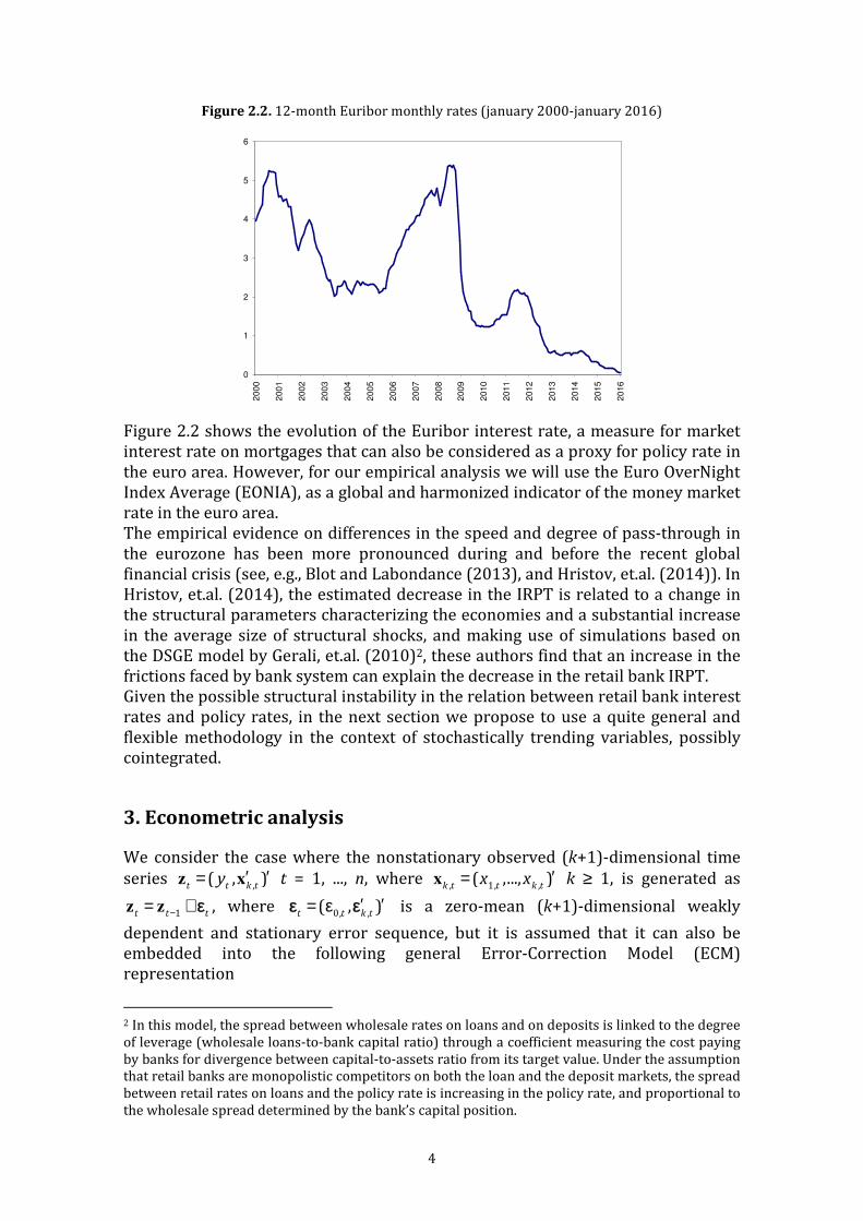
Figure 2.2. 12-month Euribor monthly rates (january 2000-january 2016)
0
1
2
3
4
5
6
20
00
20
01
20
02
20
03
20
04
20
05
20
06
20
07
20
08
20
09
20
10
20
11
20
12
20
13
20
14
20
15
20
16
Figure 2.2 shows the evolution of the Euribor interest rate, a measure for market
interest rate on mortgages that can also be considered as a proxy for policy rate in
the euro area. However, for our empirical analysis we will use the Euro OverNight
Index Average (EONIA), as a global and harmonized indicator of the money market
rate in the euro area.
The empirical evidence on differences in the speed and degree of pass-through in
the eurozone has been more pronounced during and before the recent global
financial crisis (see, e.g., Blot and Labondance (2013), and Hristov, et.al. (2014)). In
Hristov, et.al. (2014), the estimated decrease in the IRPT is related to a change in
the structural parameters characterizing the economies and a substantial increase
in the average size of structural shocks, and making use of simulations based on
the DSGE model by Gerali, et.al. (2010)2, these authors find that an increase in the
frictions faced by bank system can explain the decrease in the retail bank IRPT.
Given the possible structural instability in the relation between retail bank interest
rates and policy rates, in the next section we propose to use a quite general and
flexible methodology in the context of stochastically trending variables, possibly
cointegrated.
3. Econometric analysis
We consider the case where the nonstationary observed (k+1)-dimensional time
series ,
( , )t t k t
y ′ ′=z x t = 1, ..., n, where , 1, ,
( ,..., )k t t k t
x x ′=x k ≥ 1, is generated as
1t t t−= +z z ε , where 0, ,
( , )t t k t
′ ′= εε ε is a zero-mean (k+1)-dimensional weakly
dependent and stationary error sequence, but it is assumed that it can also be
embedded into the following general Error-Correction Model (ECM)
representation
2 In this model, the spread between wholesale rates on loans and on deposits is linked to the degree
of leverage (wholesale loans-to-bank capital ratio) through a coefficient measuring the cost paying
by banks for divergence between capital-to-assets ratio from its target value. Under the assumption
that retail banks are monopolistic competitors on both the loan and the deposit markets, the spread
between retail rates on loans and the policy rate is increasing in the policy rate, and proportional to
the wholesale spread determined by the bank’s capital position.

5
1( )[(1 ) ( 1) ]
k t t tL L L+ ′− − α − =ɶ I z eΦ λκ (3.1)
where 1,( ) ( ) k tL L +=ɶ MΦ Φ , with 1 1( ) m j
k j jL L+ == −IΦ Φ a stationary matrix
polynomial of finite order m in the lag operator L (i.e. | ( )zΦ | = 0 has roots outside
the unit circle), 0
( , )k′ ′= λλ λ ,
,(1, )
t k t′ ′= −κ β and the k+1 square matrix
1,k t+M can be
either the identity matrix or, more generally, be defined as a time-varying rotation
matrix of the form
,
1,,
1 k t
k tk k k
+
′− =
M0 I
β (3.2)
thus preserving the equivalence of the roots of each lag polynomial, with ,k tβ the k-
dimensional single time-varying cointegrating vector. For the last term in (3.1),
0, ,( , )
t t k te ′ ′=e e , it is assumed to be a zero-mean iid sequence with finite covariance
matrix [ ] 0e t t
E ′= >e eΣ , and 2+[|| || ]t
E δ < ∞e for some δ > 0. This is a modified version
of the ECM representation used in Elliott et.al. (2005) to derive a family of optimal
testing procedures for cointegration in the case of a known and time-invariant
cointegrating vector, , ,0k t k
=β β t = 1, ..., n. Taking (3.2), equation (3.1) can also be
rewritten as
1,
( 1)t t tt t t
k t k−
′ ′∆ ′= α − + ∆
zz
x
κ κ λκ ξ
λ (3.3)
with ,
( , ) ( )t t k t t
L′ ′= υ = C eξ ε , 1
0( ) ( ) j
j jL L L− ∞== =C CΦ , and
, ,t t t t k t k tu y′ ′= = −z xκ β the
cointegrating error term. Under the summability condition 1 ( )j j jjTr∞= ′ < ∞C C and
the properties of the error sequence t
e , the process tξ satisfy a multivariate
invariance principle such as
[ ] [ ]1/2 1/2 1/2
,1 1
( )( ) ( )
( )
nr nrt
tk t kt t
B rn n r r
r− − υ
ξ ξ= =
υ = = =
B WB ξξ Ωε
with (1) (1)e
′= C CξΩ Σ the long-run covariance matrix of tξ , and
( ) ( ( ), ( ))k
r W r rξ υ ′ ′=W W a k+1-variate standard Brownian process. Given that
1t t t t tu −′ ′∆ = ∆ − ∆z zκ κ , and
1 1 1t t t t tu− − −′ ′= + ∆z zκ κ with
,(0, )
t k t′ ′∆ = ∆κ β , then the first
component of the vector in (3.3) allows to represent t
u as a time-varying AR(1)
process 1 1
( )t t t t t t
u u − −′= ρ + ∆ + υzκ , where the time-varying autoregressive
coefficient is given by 1 ( 1) (1 )(1 )t t t
′ ′ρ = + α − α + − α −κ λ = κ λ , that becomes fixed in
the case of a time-invariant cointegrating vector, i.e. (1, )t k
′ ′= = −κ κ β , or,
alternatively, under the normalization restriction 1t′ =κ λ , in which case
tρ = α .
Under this last condition we obtain the following static time-varying cointegrating
regression model (a generalization of the so-called Phillip’s triangular model)
given by
6
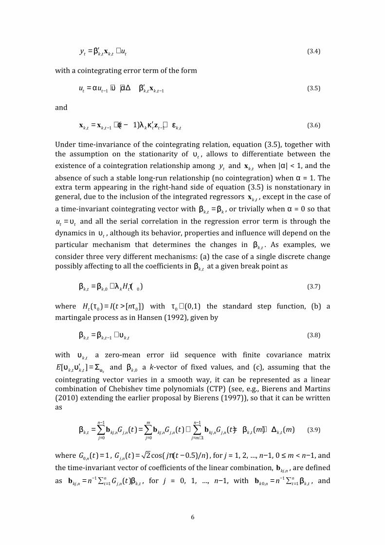
, ,t k t k t ty u′= +xβ (3.4)
with a cointegrating error term of the form
1 , , 1t t t k t k tu u − −′= α + υ + α∆ xβ (3.5)
and
, , 1 1 ,( 1)
k t k t k t t k t− −′= + α − +x x zλ κ ε (3.6)
Under time-invariance of the cointegrating relation, equation (3.5), together with
the assumption on the stationarity of t
υ , allows to differentiate between the
existence of a cointegration relationship among t
y and ,k t
x when |α| < 1, and the
absence of such a stable long-run relationship (no cointegration) when α = 1. The
extra term appearing in the right-hand side of equation (3.5) is nonstationary in
general, due to the inclusion of the integrated regressors ,k t
x , except in the case of
a time-invariant cointegrating vector with ,k t k
=β β , or trivially when α = 0 so that
t tu = υ and all the serial correlation in the regression error term is through the
dynamics in t
υ , although its behavior, properties and influence will depend on the
particular mechanism that determines the changes in ,k tβ . As examples, we
consider three very different mechanisms: (a) the case of a single discrete change
possibly affecting to all the coefficients in ,k tβ at a given break point as
, ,0 0( )
k t k k tH= + τβ β λ (3.7)
where 0 0
( ) ( [ ])t
H I t nτ = > τ with 0
(0,1)τ ∈ the standard step function, (b) a
martingale process as in Hansen (1992), given by
, , 1 ,k t k t k t−= +β β υ (3.8)
with ,k tυ a zero-mean error iid sequence with finite covariance matrix
, ,[ ]
kk t k tE ′ = υυ υ Σ and
,0kβ a k-vector of fixed values, and (c), assuming that the
cointegrating vector varies in a smooth way, it can be represented as a linear
combination of Chebishev time polynomials (CTP) (see, e.g., Bierens and Martins
(2010) extending the earlier proposal by Bierens (1997)), so that it can be written
as
1 1
, , , , , , , , ,
0 0 1
( ) ( ) ( ) ( ) ( )n m n
k t kj n j n kj n j n kj n j n k t k t
j j j m
G t G t G t m m− −
= = = +
= = + = + β β ∆b b b (3.9)
where 0,
( ) 1n
G t = , , ( ) 2cos( ( 0.5)/ )j nG t j t n= π − , for j = 1, 2, …, n−1, 0 ≤ m < n−1, and
the time-invariant vector of coefficients of the linear combination, ,kj n
b , are defined
as 1
, 1 , ,( )n
kj n t j n k tn G t−== b β , for j = 0, 1, …, n−1, with 1
0, 1 ,
n
k n t k tn−== b β , and

7
1
, 1 , ( )n
kj n k t j n kn G t−== = 0b β in the case of constancy of the cointegrating vector, i.e.
,k t k=β β for all t = 1, …, n, by the properties of the CTPs (see Appendix A for more
details). The practical use of (3.9) requires the choice of the approximation order,
m, in such a way that ,( )
k tmβ is flexible enough to approximate the pattern of
smooth variation of ,k tβ , implying that the remaining term
,( )
k tm∆ could vanish
asymptotically.3
First, under the stationarity condition on the regression error term given by |α| < 1
the scaled partial sum of t
u can be written as
[ ] [ ] [ ]1/2 1/2 1/2 1/2
0 [ ] , , 1
1 1 1
1 ( )1
nr nr nr
t t nr k t k t
t t t
n u n n u u n− − − −−
= = =
′= υ + α − + α ∆ − α xβ (3.10)
where 1/2
1 , , 1
t
j k j k jn−= −′ ∆ xβ is (1)
pO in the cases (a) and (c), while that it is 1/2( )pO n
in the case (b), and hence diverging with the sample size. Specifically we obtain
0
0
0
[ ][ ] [ ]1/2 1/2 1/2
, , 1 ,[ ] , , 0
1 1 1
[ ]1/2
,0 , 0
1
1/2
,[ ] 0
( )
( )
( ),
nnr nr
k t k t k k nr k t k t
t t t
n
k k k t
t
k k n
n n n I r
n I r
n I r
τ− − −
−= = =
τ−
=
−τ
′ ′∆ = − − > τ
′= + > τ
′= > τ
x x
x
x
β λ ε ε
λ ε
λ
(3.11)
[ ] [ ]1/2 1/2 1/2
, , 1 , 1 ,
1 1
( )nr nr
k t k t k t k t p
t t
n n O n− −− −
= =
′ ′∆ = = x xβ υ (3.12)
with
[ ]1
, 1 , , ,0
1 1
( ) ( ) [ ]k
nrr
k t k t k k t h k t
t h
n s d s r E∞
−− υ −
= =
′ ′ ′ + x B Bυ ε υ
and
[ ] [ ]1/2 3/2 1 1/2
, , 1 , , , , ,[ ]
1 1 1
[ ]1 3/2
, , 1
1 1
( ) ([ ])
( )
nr nrm
k t k t kj n j n k t j n k nr
t j t
nrm
kj n k t
j t
n j n H t n H nr n
O n n
− − − −−
= = =
− −−
= =
′ ′∆ = −π −
′+
x b x x
b x
β
(3.13)
3 See Lemma 1 in Bierens and Martins (2010), where it is precisely introduced the smoothness
condition on ,k tβ ensuring the quality of the approximation by the finite-order linear combination
in , 0 , ,( ) ( )m
k t j kj n j nm G t== bβ for some fixed natural number m < n−1. See also Theorem 2 in Martins
(2013) for a technical condition of this type when this approach is used to testing for coefficient
constancy in a stationary univariate AR(1) process.

8
respectively, where , ( ) 2sin( ( 05)/ )j nH r j t n= π − in (3.13) for j = 1, …, m. On the
other hand, under no stationarity of the regression error term in (3.4) with α = 1,
we get the representation
1/2 1/2 1/2 1/2
0 , , 1
1 1
t t
t j k j k j
j j
n u n u n n− − − −−
= =
′= + υ + ∆ xβ (3.14)
where , ,k t k t
= ∆xε , with 1/2 1/2 [ ] 1/2
[ ] 1 ( ) ( )nr
nr t t pn u n O n B r− − −= υ= υ + , under time
invariance of the regression coefficients and the usual assumption of the initial
value 0
(1)p
u O= , where the last term 1/2
1 , , 1
t
j k j k jn−= −′ ∆ xβ is given as in (3.11)-
(3.13). Thus, assuming the validity of the time-varying ECM representation in (3.1),
the cointegration assumption implies the extra condition α = 0, while that under
no cointegration the disequilibrium error term t
u contains an additional term
incorporating the changes in the values of ,k tβ , whenever it has a clear definition.
Also, as can be seen from (3.6), the assumption that ,k t
x are not mutually
cointegrated and have roots that are known a priori to be equal to one (i.e. ,k t
x are
k ≥ 1 integrated but not-cointegrated regressors), corresponds to the restriction
k k= 0λ (which implies
01λ = ), and hence (3.6) must be replaced by the usual
representation as a k-dimensional integrated process4
, , 1 ,k t k t k t−= +x x ε (3.6´)
which also results in the case of no cointegration, i.e. when α = 1 in (3.5),
irrespective of the value of kλ . A second form of the model is the ECM
representation (3.1) with ( )LɶΦ replaced by ( )LΦ , i.e.
1( ) ( 1) ( )
t t t tL L −′∆ = α − +z z eΦ Φ λκ , that can be written as a time-varying reduced
rank ECM of the form
1 1( 1) (1) ( )
t t t t t tL− −′∆ = α − + ∆ +z z z eΦ λκ Λ (3.15)
by making use of the BN decomposition *( ) (1) (1 ) ( )L L L= + −Φ Φ Φ where * * 1
1( ) m j
j jL L −==Φ Φ and * m
j i j i==Φ Φ , with the lag polynomial 1
0 ,( ) m j
t j j tL L−==Λ Λ and
time-varying coefficients *
, 1 1( 1)j t j t j+ +′= α − +Λ Φ λκ Φ , unless t
=κ κ or, alternatively,
α = 1 irrespective of the behaviour of tκ . Under the restrictions considered we
4 By recursive substitutions, equation (4.6) can also be written as
, ,0 1 ,
t
k t k j k j== + +x x ε
1 1( 1) t
k j j j= −′α − zλ κ , where the last term is decomposed as 1 1 1 1 1 1
t t t
j j j j j j j ju= − = − = −′ ′ = + ∆z zκ κ , with
t t tu ′= zκ . With a fixed cointegrating vector,
t=κ κ ,
1 10t
j j j= −′ ∆ =zκ , while that with a time-varying
cointegrating vector we have the representation 1 1 1 , , ,0 ,0 , ,
( )t t
j j j j k j k j k k k t k t= − =′ ′ ′ ′ ∆ = − − −z x xκ β ε β β . In
the fixed parameter case and under cointegration we get 1/ 2
,( ) ( 1) ( )
k t k k un r B r− + α −x B λ , with t =
[nr], r ∈ (n−1,1], and 1( ) (1 ) ( )u
B r B r−υ= − α as n→∞, while that under no cointegration the weak limit
is 1/ 2
,( )
k t kn r− x B , implying a different behavior in each situation that is unlikely in any real
analysis.
9
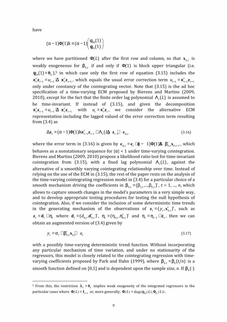
have
00
0
(1)( 1) (1) ( 1)
(1)k
φ α − α −
Φ λ =φ
where we have partitioned ( )LΦ after the first row and column, so that ,k t
x is
weakly exogeneous for ,k tβ if and only if (1)Φ is block upper triangular (i.e.
0(1)
k k= 0φ ),5 in which case only the first row of equation (3.15) includes the
1 1 1t t t t tu− − −′ ′= + ∆z zκ κ , which equals the usual error correction term
1 1 1t t tu − − −′= zκ
only under constancy of the cointegrating vector. Note that (3.15) is the ad hoc
specification of a time-varying ECM proposed by Bierens and Martins (2009,
2010), except for the fact that the finite order lag polynomial ( )t
LΛ is assumed to
be time-invariant. If instead of (3.15), and given the decomposition
1 1 1t t t t tu− − −′ ′= + ∆z zκ κ with
t t tu ′= zκ , we consider the alternative ECM
representation including the lagged valued of the error correction term resulting
from (3.4) as
1 1 1 ,( 1) (1) ( )
t t t t t tL− − − α′∆ = α − + ∆ +z z z eΦ λκ Λ (3.16)
where the error term in (3.16) is given by , , , 1
( 1) (1)t t k t k tα −′= + α − ∆e e xΦ λ β , which
behaves as a nonstationary sequence for |α| < 1 under time-varying cointegration.
Bierens and Martins (2009, 2010) propose a likelihood ratio test for time-invariant
cointegration from (3.15), with a fixed lag polynomial ( )t
LΛ , against the
alternative of a smoothly varying cointegrating relationship over time. Instead of
relying on the use of the ECM in (3.15), the rest of the paper rests on the analysis of
the time-varying cointegrating regression model in (3.4) for a particular choice of a
smooth mechanism driving the coefficients in , 1, ,
( ,..., )k t t k t
′= β ββ , t = 1, ..., n, which
allows to capture smooth changes in the model’s parameters in a very simple way,
and to develop appropriate testing procedures for testing the null hypothesis of
cointegration. Also, if we consider the inclusion of some deterministic time trends
in the generating mechanism of the observations of ,
( , )t t k t
y ′ ′=z x , such as
t t t= +z d η where
0, ,( , )
t t k td ′ ′=d d ,
0, ,( , )
t t k t′ ′= ηη η and
1t t t−= +η η ε , then we can
obtain an augmented version of (3.4) given by
, ,t t k t k t ty u′= α + +xβ (3.17)
with a possibly time-varying deterministic trend function. Without incorporating
any particular mechanism of time variation, and under no stationarity of the
regressors, this model is closely related to the cointegrating regression with time-
varying coefficients proposed by Park and Hahn (1999), where ,
( / )k t k
t n=β β is a
smooth function defined on [0,1] and is dependent upon the sample size, n. If (·)kβ
5 From this, the restriction
k k= 0λ implies weak exogeneity of the integrated regressors in the
particular cases where 1
( )k
L += IΦ or, more generally, 00
( ) diag( ( ), ( ))kk
L L L= φΦ Φ .

10
is sufficiently smooth, the estimand 1
( ) ( ( ),..., ( ))m k k k m
r r′ ′ ′=Π β β β , with [0,1]j
r ∈ , j = 1,
…, m, m ≥ 1, may be approximated by a series of polynomial and/or trigonometric
functions on [0,1]. The authors propose the trigonometric pairs
(cos(2 / ),sin(2 / ))jt T jt Tπ π , j = 1, 2, …, m, to obtain this approximate representation
and formulate a technical condition ensuring a rate of convergence for sufficiently
large m.6 We follow the same idea but propose the use of a set of different
approximating functions based on the Chebyshev time polynomials.
4. Empirical analysis
In this section we focus on the analysis of the time-varying cointegrating
relationship among the retail interest rates for different maturities and two
definitions of credit variables, namely credits for house purchase and loans for
consumption, to evaluate the magnitude of the long-run IRPT for a subset of
countries in the Euro Area for which the longest and complete series is available.
As argued in Belke et.al. (2013), when analyzing aggregated micro data from many
banks, each of these institutions might face different information and transaction
costs, a smooth transition pattern seems to be a plausible mechanism. These
authors use a smooth transition regression to incorporate different patterns of
nonlinearity in the adjustment and short-run dynamics for the relationship
between the Euro OverNight Index Average (EONIA), as a global indicator of the
money market rate in the Euro Area, and credit categories with various maturities.
Marotta (2009) considers the possibility of allowing for multiple unknown
structural breaks in the cointegrating relationship based on unharmonized retail
rates for several EMU countries, and found different estimates of the equilibrium
pass-through indicating a slow adjustment to the monetary regimes. From these
results and the evidence presented in ECB (2009), indicating no evidence for a
structural change in the IRPT mechanism during the recent period of the financial
crisis, instead of relying of these particular choices for explaining the possible
variability of the magnitude of the long-run relationship between the retail and the
market interest rates we consider the more flexible and general approach based on
the assumption of time-varying parameters in the cointegrating regression model
modelled as a weighted average of Chebyshev time polynomials with deterministic
weights, following the proposal by Bierens (1997). For a formal description of this
approach and some important results arising from fitting a time-varying
cointegrating regression model via Chebyshev time polynomials see Appendix A.
Next we describe the data used in the empirical analysis and the structure of the
econometric study.
4.1. The data and some initial basic results
Following Belke et.al. (2013), for the harmonized retail rates data we use the
harmonized interest rate series from the Monetary Financial Institutions (MFI)
interest rate statistics of the European Central Bank (ECB) for the seven countries
and periods appearing in Table 1, representing the longest series for which
complete data are available. All data refer to loans for households and non-profit
6 See Lemma 2, p. 668, in Park and Hahn (1999).

11
institutions and are monthly averages and exclusively new business. For the credit
categories we consider credits for house purchase and loans for consumption with
short, medium and long maturities (up to 1 year, over 1 and up to 5 years, and over
5 years, respectively).
Table 1. Monthly retail rates by country
Credits for house purchase Loans for consumption
Country Period n Period n
Austria 01.2003-12.2014 144 01.2000-12.2014 180
Belgium 10.2006-12.2014 99 10.2006-12.2014 99
Finland 01.2003-12.2014 144 01.2000-12.2014 180
France ″ ″ ″ ″
Germany ″ ″ ″ ″
Italy ″ ″ 01.2003-12.2014 144
Spain ″ ″ 01.2000-12.2014 180
As the money market rate for all the countries we consider the EONIA,7 because it
seems to better reflect the stance of the monetary policy. Figure 4.1 shows monthly
series of the EONIA and the three-month Effective Federal Funds Rates (EFFR) as a
proxy for the policy rate in the US economy, which can be described as a market-
based system as opposed to the bank-based system for the Euro Area, for the
period january 1999 to december 2014. The time path of both series closely
resembles, displaying an apparent nonstationary behavior but with a certain time
delay in the response of the EONIA rates to changes in the EFFR. Cross
contemporaneous correlation between both series in first differences is 0.358,
while cross autocorrelations are 0.41, 0.402 and 0.332 for lags 1-3 of the EFFR
series.
Figure 4.1. Monthly EONIA and Effective Federal Funds Rates (01.1999-12.2014) in levels (left)
and in first differences (right)
-1.000
0.000
1.000
2.000
3.000
4.000
5.000
6.000
7.000
19
99
20
00
20
01
20
02
20
03
20
04
20
05
20
06
20
07
20
08
20
09
20
10
20
11
20
12
20
13
20
14
20
15
EONIA FedFunds rate
-1.200
-1.000
-0.800
-0.600
-0.400
-0.200
0.000
0.200
0.400
0.600
19
99
20
00
20
01
20
02
20
03
20
04
20
05
20
06
20
07
20
08
20
09
20
10
20
11
20
12
20
13
20
14
EONIA FedFunds rate
Next, figures 4.2-4.8 show the time pattern of the retail interest rates for each of
the seven countries for both types of credit categories and the three maturities
7 EONIA is the effective overnight reference rate for the euro computed as a weighted average of all
overnight unsecured lending transactions in the interbank market undertaken in the EMU and
European Free Trade Association (EFTA) countries.

12
considered in the analysis.
Figure 4.2. Retail rates of credits for house purchase (left) and loans for consumption (right): Austria
0
1
2
3
4
5
6
7
2003 2004 2005 2006 2007 2008 2009 2010 2011 2012 2013 2014
up to 1 year over 1 and up to 5 years over 5 years
0
1
2
3
4
5
6
7
8
9
2000 2001 2002 2003 2004 2005 2006 2007 2008 2009 2010 2011 2012 2013 2014
up to 1 year over 1 and up to 5 years over 5 years
Figure 4.3. Retail rates of credits for house purchase (left) and loans for consumption (right):
Belgium
0
1
2
3
4
5
6
7
20062007 2008 2009 2010 2011 2012 2013 2014
up to 1 year over 1 and up to 5 years over 5 years
0
2
4
6
8
10
12
20062007 2008 2009 2010 2011 2012 2013 2014
up to 1 year over 1 and up to 5 years over 5 years
Figure 4.4. Retail rates of credits for house purchase (left) and loans for consumption (right): Finland
0
1
2
3
4
5
6
2003 2004 2005 2006 2007 2008 2009 2010 2011 2012 2013 2014
up to 1 year over 1 and up to 5 years over 5 years
0
2
4
6
8
10
12
14
16
18
2000 2001 2002 2003 2004 2005 2006 2007 2008 2009 2010 2011 2012 2013 2014
up to 1 year over 1 and up to 5 years over 5 years
Figure 4.5. Retail rates of credits for house purchase (left) and loans for consumption (right): France
0
1
2
3
4
5
6
2003 2004 2005 2006 2007 2008 2009 2010 2011 2012 2013 2014
up to 1 year over 1 and up to 5 years over 5 years
0
1
2
3
4
5
6
7
8
9
10
2000 2001 2002 2003 2004 2005 2006 2007 2008 2009 2010 2011 2012 2013 2014
up to 1 year over 1 and up to 5 years over 5 years

13
Figure 4.6. Retail rates of credits for house purchase (left) and loans for consumption (right):
Germany
0
1
2
3
4
5
6
7
2003 2004 2005 2006 2007 2008 2009 2010 2011 2012 2013 2014
up to 1 year over 1 and up to 5 years over 5 years
0
1
2
3
4
5
6
7
8
9
10
2000 2001 2002 2003 2004 2005 2006 2007 2008 2009 2010 2011 2012 2013 2014
up to 1 year over 1 and up to 5 years over 5 years
Figure 4.7. Retail rates of credits for house purchase (left) and loans for consumption (right): Italy
0
1
2
3
4
5
6
7
8
2003 2004 2005 2006 2007 2008 2009 2010 2011 2012 2013 2014
up to 1 year over 1 and up to 5 years over 5 years
0
2
4
6
8
10
12
14
2003 2004 2005 2006 2007 2008 2009 2010 2011 2012 2013 2014
up to 1 year over 1 and up to 5 years over 5 years
Figure 4.8. Retail rates of credits for house purchase (left) and loans for consumption (right): Spain
0
2
4
6
8
10
12
2003 2004 2005 2006 2007 2008 2009 2010 2011 2012 2013 2014
up to 1 year over 1 and up to 5 years over 5 years
0
2
4
6
8
10
12
14
2000 2001 2002 2003 2004 2005 2006 2007 2008 2009 2010 2011 2012 2013 2014
up to 1 year over 1 and up to 5 years over 5 years
Simple visual inspection of all these series reveals a very different behavior of the
retail credit markets in each country in the sample, with a certain homogeneity
among maturities for each economy and credit category. Particularly interesting in
the case of Spain, where the series of interest rates for house purchase and short-
term maturity has experienced a wide growth from 2013, while the short-term
rate of loans for consumption displays a sharp fall at the end of 2010, and has
remained since then between 6 and 8% which is the highest value for the seven
countries. These different behaviours seems to anticipate the differences
encountered in practice in the estimation of the magnitude of the short and long-
run IRPT measures, but can also serve as a justification for the use of a flexible
modelling such as the one considered in this paper. The main tool proposed to the

14
analysis of the mechanism of transmission of the monetary policy from the money
to the retail markets is a simple regression model of the form
t t ty x u= α +β + (4.1)
that falls into the class of cointegrating regression models given the no stationary
behavior of the series involved, with the dependent variable, t
y , given by the retail
rate for different maturities of the credit for house purchase and loans for
consumption as credit categories, and explanatory variable, t
x , given by the EONIA
interest rate. The results of the analysis of integration and stationarity for all the
series are not presented here,8 but strongly indicates that the variables are no
stationary, thus supporting the analysis of the regression model as a way of
representing the cointegrating relationship among the retail interest rates and the
money market rate. Table E.1 in Appendix E presents the results of a variety of
testing procedures for cointegration, roughly indicating the no existence of a stable
long-run relationship in all the cases when based on the time-invariant regression
model (4.1). One possible explanation for these results could be attributed to the
existence of a time-varying stable relationship omitted in (4.1), as is apparent from
the results of Hansen’s (1992) tests for parameter instability in cointegration
regressions with integrated regressors.9 Appendix A contains the theoretical
analysis of the consistency of this testing procedure against the alternative of a
time-varying cointegrating regression where the pattern of changes in the
parameters is modelled via Chebyshev time polynomials. This is the approach
taken in the rest of this section.
4.2. Time-varying cointegrating regression analysis
With the aim to explore the capability of the approach proposed by Bierens (1997),
and extended by Bierens and Martins (2009, 2010) and Neto (2012, 2014) to the
cointegration analysis, we propose the following generalization of equation (4.1)
as
( ) ( )t t t t t
y m m x u= α + β + (4.2)
where the time-varying intercept and slope are defined as
, ,
0
( ) ( )m
t j n j n
j
m a G t=
α = (4.3)
and
8 The analysis was performed based on the usual ADF and PP test statistics for the null of
integration against the alternative of stationarity, and the KPSS test statistic for the hypothesis in
reverse order. In all the cases, the stationarity hypothesis is rejected at the 5% level of signification. 9 Quintos and Phillips (1993) also propose a number of related procedures to test the null
hypothesis of time-invariant cointegration against specific directions of departures from the null,
including the possibility to test the stability of a subset of coefficients. For more results related to
testing for partial parameter instability in cointegrating regressions see also Kuo (1998) and Hsu
(2008).

15
, ,
0
( ) ( )m
t j n j n
j
m b G t=
β = (4.4)
respectively, with 0,
( ) 1n
G t = , , ( ) 2cos( ( 0.5)/ )j nG t j t n= π − , j = 1, 2, ..., m, m ≤ n−1.
This general specification allows to obtain three alternative models given by
Model 1. No intercept and TV slope, ,
0j n
a = , j = 0, 1, ..., m
Model 2. Fixed intercept and TV slope, ,
0j n
a = , j = 1, ..., m
and
Model 3. TV intercept and slope.
This model does not allow to capture in general structural changes in the
cointegrating relationship since the functions ( )t
mα and ( )t
mβ are assumed to be
smooth and slow time-varying deterministic functions of time. However, there
exists the possibility of easily combine the proposed formulation with a structural
break, unless the magnitude shifts be small enough to be subsumed by the time-
varying structure of the model parameters, as shown in the analysis of Appendix B.
The analysis performed in this section based on (4.2)-(4.3) requires the OLS
estimation of the coefficients , ,
,j n j n
a b j = 0, 1, ..., m for a particular choice of 1 ≤ m <
n, and the computation of the test statistics
2
2 21 1,
1ˆ ˆ( ) ( )ˆ ( )
n t
n j
t ju n n
K m u mn q = =
= ω
(4.5)
and
1,...,
1,
1ˆ ˆ( ) max ( )ˆ ( )
t
n t n j
ju n n
CS m u mq n =
==
ω (4.6)
where 2 2
, , ,ˆˆ ˆ( ) 2 ( )
u n n u n u n nq qω = σ + λ is a kernel-type estimator of the long-run variance
of t
u , with 2 1 2
, 1ˆˆ ( )n
u n t tn u m−=σ = and 1 1
, 1 1ˆ ˆ ˆ( ) ( / ) ( ) ( )n n
u n n h n t h t h tq w h q n u m u m− −
= = + −λ = for
some weighting function w(·) and bandwidth 1/2( )n
q o n= , based on the
autocovariances of the residuals
, , , , ,
0
1ˆˆˆ ( ) (( ),( )) ( )m
t t j n j n j n j n j ntj
u m u a a b b G tx=
= − − −
The statistic (4.5) is the so-called KPSS test statistic for testing the null hypothesis
of stationarity for the regression error term t
u , and hence cointegration, while that
ˆ ( )n
CS m in (4.6) is the Xiao and Phillips (2002) test statistic adapted to the
residuals from (4.2) as has been considered by Neto (2014). In the case of
endogeneous regressors, the OLS version of these test statistics cannot be used in
practical applications given that their limiting null distributions depend on some
nuisance parameters, and hence must be computed on the basis of residuals from
some asymptotically efficient estimation such as the FM-OLS method (see Neto
16
(2014) and Appendix B). Table D.1 in Appendix D contains the finite-sample upper
critical values for Models 1-3 with one integrated regressor and m = 1, …, 5, thus
generalizing the results in Neto (2014). The limiting null distribution of these test
statistics is model-dependent in the sense that the critical values differ for each
model and value of m. To avoid this dependence on the model specification and
dimension when testing for time-varying cointegration, we also propose the use of
the test statistics proposed by McCabe et.al. (2006) (MLH) described in Appendix
C, which also have the advantages of relying only on the OLS estimation of the
time-varying cointegrating regression (4.2), even under endogeneity of the
integrated regressors.
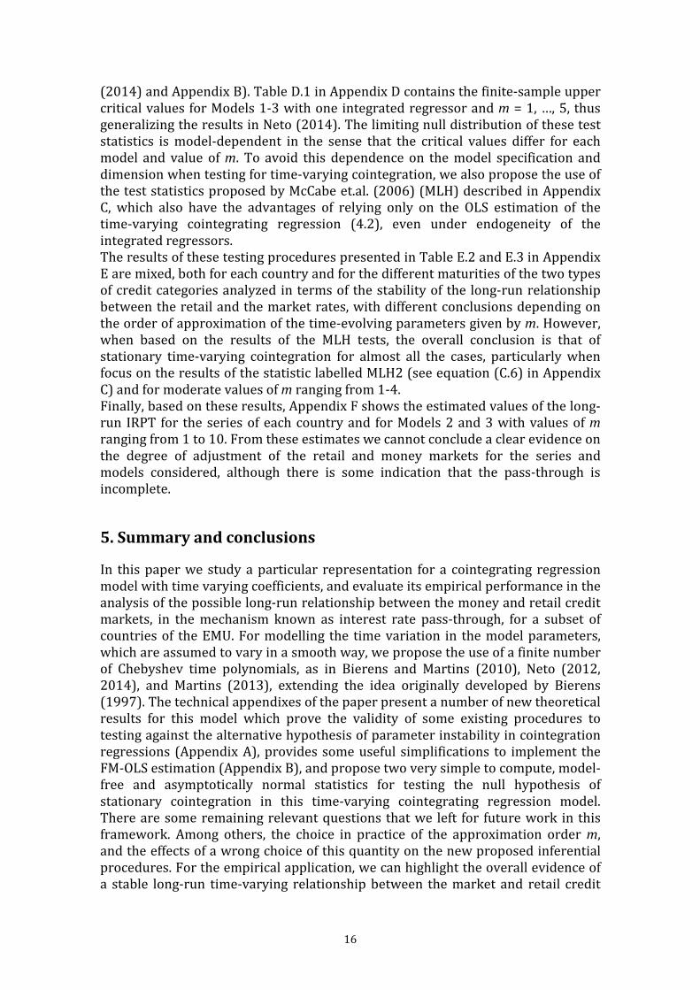
The results of these testing procedures presented in Table E.2 and E.3 in Appendix
E are mixed, both for each country and for the different maturities of the two types
of credit categories analyzed in terms of the stability of the long-run relationship
between the retail and the market rates, with different conclusions depending on
the order of approximation of the time-evolving parameters given by m. However,
when based on the results of the MLH tests, the overall conclusion is that of
stationary time-varying cointegration for almost all the cases, particularly when
focus on the results of the statistic labelled MLH2 (see equation (C.6) in Appendix
C) and for moderate values of m ranging from 1-4.
Finally, based on these results, Appendix F shows the estimated values of the long-
run IRPT for the series of each country and for Models 2 and 3 with values of m
ranging from 1 to 10. From these estimates we cannot conclude a clear evidence on
the degree of adjustment of the retail and money markets for the series and
models considered, although there is some indication that the pass-through is
incomplete.
5. Summary and conclusions
In this paper we study a particular representation for a cointegrating regression
model with time varying coefficients, and evaluate its empirical performance in the
analysis of the possible long-run relationship between the money and retail credit
markets, in the mechanism known as interest rate pass-through, for a subset of
countries of the EMU. For modelling the time variation in the model parameters,
which are assumed to vary in a smooth way, we propose the use of a finite number
of Chebyshev time polynomials, as in Bierens and Martins (2010), Neto (2012,
2014), and Martins (2013), extending the idea originally developed by Bierens
(1997). The technical appendixes of the paper present a number of new theoretical
results for this model which prove the validity of some existing procedures to
testing against the alternative hypothesis of parameter instability in cointegration
regressions (Appendix A), provides some useful simplifications to implement the
FM-OLS estimation (Appendix B), and propose two very simple to compute, model-
free and asymptotically normal statistics for testing the null hypothesis of
stationary cointegration in this time-varying cointegrating regression model.
There are some remaining relevant questions that we left for future work in this
framework. Among others, the choice in practice of the approximation order m,
and the effects of a wrong choice of this quantity on the new proposed inferential
procedures. For the empirical application, we can highlight the overall evidence of
a stable long-run time-varying relationship between the market and retail credit

17
interest rates considered in this study. However, the point estimates of the long-
run IRPT show evidence of incomplete pass-through between these series.
References
Belke, A., J. Beckmann, F. Verheyen (2013). Interest rate pass-through in the EMU – New
evidence from nonlinear cointegration techniques for fully harmonized data. Journal of
International Money and Finance, 37(1), 1-24.
Bernanke, B.S., A.S. Blinder (1992). The federal funds rate and the channels of monetary
transmission. American Economic Review, 82(4), 901-921.
Bierens, H.J. (1997). Testing the unit root with hypothesis against nonlinear trend
stationarity, with an application to the US price level and interest rate. Journal of
Econometrics, 81(1), 29-64.
Bierens, H.J., L.F. Martins (2009). Appendix: Time varying cointegration.
http://econ.la.psu.edu/∼hbierens/TVCOINT_APPENDIX.PDF.
Bierens, H.J., L.F. Martins (2010). Time-varying cointegration. Econometric Theory, 26(5),
1453-1490.
Blot, C., F. Labondance (2013). Bank interest rate pass-through in the eurozone: monetary
policy transmission during the boom and since the financial crash. Economics Bulletin,
33(2), 973-985.
Borio, C.E.V., W. Fritz (1995). The response of short-term bank lending rates to policy
rates: a cross-country perspective. BIS Working Paper No.27.
Cottarelli, C., A. Kourelis (1994). Financial structure, bank lending rates, and the
transmission mechanism of monetary policy. IMF Staff Papers, 41(4), 587-623.
de Bondt, G.J. (2005b). Interest rate pass-through: empirical results for the euro area.
German Economic Review, 6(1), 37-38.
de Bondt, G.J., B. Mojon, N. Valla (2005a). Term structure and the sluggishness of retail
bank interest rates in euro area countries. ECB Working Paper No.518.
ECB (2009). Recent developments in the retail bank interest rate pass-through in the euro
area. ECB Monthly Bulletin, august, 93-105.
Elliott, G., M. Jansson, E. Pesavento (2005). Optimal power for testing potential
cointegrating vectors with known parameters for nonstationarity. Journal of Business
and Economic Statistics, 23(1), 34-48.
Fernández de Lis, S., J.F. Izquierdo, A. Rubio (2015). Determinantes del tipo de interés del
crédito a empresas en la Eurozona. BBVA Research, Working Paper No.15/09.
Gerali, A., S. Neri, L. Sessa, F.M. Signoretti (2010). Credit and banking in a DSGE model of
the euro area. Journal of Money, Credit and Banking, 42(6), 108-141.
Hansen, B.E. (1992). Tests for parameter instability in regressions with I(1) processes.
Journal of Business and Economic Statistics, 10(3), 45-59.
Hristov, N., O. Hülsewig, T. Wollmershäuser (2014). The interest rate pass-through in the
Euro area during the global financial crisis. Journal of Banking and Finance, 48, 104-
119.
Hsu, C.C. (2008). A note on tests for partial parameter stability in the cointegrated system.
Economics Letters, 99(3), 500-503.
Illes, A., M. Lombardi (2013). Interest rate pass-through since the financial crisis. BIS
Quarterly Review, September, 57-66.
Kobayashi, T. (2008). Incomplete interest rate pass-through and optimal monetary policy.
International Journal of Central Banking, 4(3), 77-118.
Kuo, B.S. (1998). Test for partial parameter instability in regressions with I(1) processes.
Journal of Econometrics, 86(2), 337-368.
Kwapil, C., J. Scharler (2010). Interest rate pass-through, monetary policy rules and
macroeconomic stability. Journal of International Money and Finance, 29(2), 236-251.
Marotta, G. (2009). Structural breaks in the lending interest rate pass-through and the
18
euro. Economic Modelling, 26(1), 191-205.
Martins, L.F. (2013). Testing for parameter constancy using Chebyshev time polynomials.
The Manchester School, 81(4), 586-598.
McCabe, B., S. Leybourne, D. Harris (2006). A residual-based test for stochastic
cointegration. Econometric Theory, 22(3), 429-456. Neto, D. (2012). Testing and estimating time-varying elasticities of Swiss gasoline demand.
Energy Economics, 34(6), 1755-1762.
Neto, D. (2014). The FMLS-based CUSUM statistic for testing the null of smooth time-
varying cointegration in the presence of a structural break. Economics Letters, 125(2),
208-211.
Park, J.Y., S.B. Hahn (1999). Cointegrating regressions with time varying coefficients.
Econometric Theory, 15(5), 664-703.
Phillips, P.C.B., B.E. Hansen (1990). Statistical inference in instrumental variables
regression with I(1) processes. The Review of Economic Studies, 57(1), 99-125.
Phillips, P.C.B., S. Ouliaris (1990). Asymptotic properties of residual based tests for
cointegration. Econometrica, 58(1), 165-193.
Quintos, C.E., P.C.B. Phillips (1993). Parameter constancy in cointegrating regressions.
Empirical Economics, 18(4), 675-706.
Shin, Y. (1994). A residual-based test of the null of cointegration against the alternative of
no cointegration. Econometric Theory, 10(1), 91-115.
Sorensen, K., T. Werner (2006). Bank interest rate pass-through in the Euro Area: a cross
country comparison. ECB Working Paper No.580.
Xiao, Z., P.C.B. Phillips (2002). A CUSUM test for cointegration using regression residuals.
Journal of Econometrics, 108(1), 43-61.

19
Appendix A. Hansen’s tests for parameter instability under time-varying
cointegrating regression via Chebyshev time polynomials
Let us assume that the time-varying cointegrating vector, , 1, ,
( ,..., )k t t k t
′= β ββ , in the
specification of the time-varying (TV) cointegrating regression model,
, ,t k t k t ty u′= +xβ , with
, ,k t k t∆ =x ε , is given by
1
, , ,
0
( )n
k t kj n j n
j
G t−
=
=β α (A.1)
where 1
, 1 , , ( )n
kj n t k t j nn G t−== α β by the orthogonality property of Chebyshev
polynomials ,
( )j n
G t , i.e., 1
1 , ,( ) ( ) ( )n
t j n i nn G t G t I i j−= = = , with
,( ) 1 0
( 0.5)2cos 1,2,..., 1
j nG t j
j tj n
n
= =
π − = = −
(A.2)
which implies that 1
1 , ( ) 0n
t j nn G t−= = for any j = 1, 2, .... Also, given that
,k tβ can be
written as , , ,
( ) ( )k t k t k t
m m= + bβ β , with
, , ,
0
( ) ( )m
k t kj n j n
j
m G t=
=β α (A.3)
for some fixed natural number m < n−1, and the fact that for the remaining term 1
, 1 , ,( ) ( )n
k t j m kj n j nm G t−= +=b α we have that 1
, 1 , ,lim ( ) ( ) 0n
m n t k t k tn m m−→∞ = ′ =b b and
1 2
1 , ,lim ( ) ( ) ( 1)n q
n t k t k tn m m m− −→∞ = ′ ≤ +b b for q ≥ 2 and m ≥ 1 (see Lemma 1 in
Bierens and Martins (2010)), then our TV cointegrating regression model is given
by
,
, , , , , 0, ,,0
( ) ( ) ( , )m
k t
t k t k t t kj n k t j n t k n km n tkm tj
y m u G t u u=
′ ′ ′ ′= + = + = +
x
x x AX
β α α (A.4)
with , 1, ,
( ,..., )km n k n km n
′ ′ ′=A α α , , 1, ,
( ,..., )km t k t km t
′ ′ ′=X x x , and , , ,
( )kj t k t j n
G t=x x , j = 1, ..., m.
The necessary tools required for the asymptotic analysis of the estimation results
arising from this specification are provided by Bierens (1997) (see Lemmas A.1-
A.5) and Bierens and Martins (2009, 2010). Thus, under the assumption that the
regression error term t
u is given by 1t t t
u u −= α + υ , with |α| ≤ 1 and t
υ a zero-mean
weakly stationary error sequence with finite variance, and defining the partial sum
process of t
u as ( ) 0n
U r = when 1[0, ]r n−∈ , and [ ]
1( ) nr
n t tU r u== for 1[ ,1]r n−∈ , then
we get [ ]
1/2
0 01
( / ) ( ) ( ) (1) (1) ( ) ( )nr
r r
t u u u
t
n F t n u F s dB s F B f s B s ds−
=
= − (A.5)
and [ ] [ ]
3/2 1 1/2
01 1
( / ) ( / ) ( / )( ( / )) ( ) ( )nr nr
r
n n u
t t
n F t n U t n n F t n n U t n F s B s ds− − −
= =
= (A.6)
where ( )u
B r is a Brownian motion process characterizing the weak limit of 1/2 ( )
nn U r− , for any differentiable real function on [0,1], F(·), with derivative f(·).
Also, given that 1/2
, [ ] ,0 , ( )k n nr k k nn r−=x x B+ , with 1/2 [ ]
, 1 ,( ) nr
k n j k jr n−== B ε for 1[ ,1]r n−∈ ,
and ,
( )k n k
r =B 0 for 1[0, ]r n−∈ , then we get that 1
1 , ,
n
t kj nt k ntn−= ′ x x and

20
1
1 , ,
n
t kj nt kj ntn−= ′ x x are both (1)
pO . Taking now
,0 0,k k n=β α , the TV cointegrating
regression can be rewritten as
,0 , , , , ,0 ,
1
( )n
t k k t t kj n k t j n k k t t
j
y u G t v=
′ ′ ′= + + = +x x xβ α β (A.7)
where , ,t t km t km n
v u ′= + X A , where the OLS estimation error of ,0kβ is given by
1
(1/2 ) 1 (1 )
0, 0 , , ,
1 1
1
(1/2 ) 1 (1 )
, , , , ,
1 1
ˆ
( )
n n
k n k k nt k nt k nt t
t t
n n
k nt k nt k nt t km nt km n
t t
n n n v
n n n u n
−− +κ − − −κ
= =
−− +κ − − −κ
= =
′− =
′ ′= +
x x x
x x x X A
β β (A.8)
with 1/2
, ,k nt k tn−=x x , 1/2
, , 1, ,( ,..., )km nt km t k nt km ntn− ′ ′ ′= =X X x x , and , , ,
( )kj nt k nt j n
G t=x x , j = 1,
..., m. Given that , , , , , , ( 1)
( ) ( ( ) ( 1))kj nt j n k t j n j n k n t
G t G t G t −∆ = + − −x xε , it comes that the
variance of ,kj nt
∆x is not constant since it depends on t, but as
2
, , ,( ) ( ) ( / ) ( ) ( )j n j n j nG t h G t hj n H t O n−+ − = − π + with , ( ) 2sin( ( 0.5)/ )j nH t j t n= π − for
each j = 1, 2, ... the second term becomes asymptotically negligible and hence 2
, , , ,[ ] ( ) [ ]kj nt j n k t k tVar G t E ′∆ →x ε ε as n→∞, that depends on t only through the
Chebyshev polynomial. The scaled OLS estimation error is then given by
1/2 1 (1 ) 1/2 1
0, 0 , , , , ,
1 1
ˆ( )n n
k n k kk n k nt t k nt km nt km n
t t
n n u n n+κ − − −κ +κ −
= =
′− = +
Q x x X Aβ β (A.9)
where 1
, 1 , ,
n
kk n t k nt k ntn−= ′= Q x x , with the index κ taking the values κ = 1/2 under
cointegration, that is when the error term t
u is stationary, and κ = −1/2 under no
cointegration, so that the second term between brackets will dominates the
behavior of 0, 0
ˆ( )k n k
n −β β under cointegration when ,km n km
≠A 0 . From this result,
the t-th OLS residual is given by 1/2 1/2
, 0, 0 , ,ˆˆ [ ( )]
t t k nt k n k t km nt km nv v n n u n−κ +κ′ ′= − − = +ɶx d Aβ β (A.10)
where the two terms composing these residuals are
1 (1 )
, , ,
1
n
t t k nt kk n k nj j
j
u u n n u−κ − − −κ
=
′= − ɶ x Q x (A.11)
and
1 1
, , , , , ,
1
n
km nt km nt km nj k nj kk n k nt
j
n− −
=
′= − d X X x Q x (A.12)
Hansen (1992) proposed a set of statistics to test for parameter instability in
regression models with integrated regressors that are based on different measures
of excessive variability of the partial sums of the estimated scores from the model
fitting. First, we consider the case of the OLS estimated scores, , ,
ˆ ˆk t k t t
v=s x , that can
be decomposed as 1/2
, , , , ,ˆ
k t k nt k nt km nt km nn n ′= +ɶs s x d A (A.13)
where , ,
(1)k nt k nt t p
u O= =ɶ ɶs x under cointegration, so that , 1 ,
ˆ ˆt
k t j k j==S s can be
written as
21
1/2 1
, , , , ,
1 1
, ( ), ,
ˆ
( )
t t
k t k nj k nj km nj km n
j j
k nt k km nt km n
n n n n
n n
− −
= =
′= +
= +
ɶ
ɶ
S s x d A
V V A
(A.14)
which implies that , ,
ˆ ( )k t k nt p
n O n= =ɶS V when ,km n km
=A 0 , where 1
,ˆ
k tn−
S has a well
defined weak limit. Under the general assumption that the model parameters ,k tβ
follow a martingale process , , 1 ,k t k t k t−= +β β η , with 2
, ,[ ]k t k t tE ′ = δ Gη η and
1 2
. ,t v k kk n
− = ωG M , where , 1 , ,
n
kk n t k t k t= ′=M x x and 2 2 1
.v k v kv kk kv
−′ω = ω − ω Ω ω is the
conditional long-run variance of t
v given the sequence of error terms driving the
integrated regressors, ,k tε , then the OLS version of the LM-type test statistic is
given by
1 1 1 1 1
, , , , , ,2 21 1, ,
1 1ˆ ˆ ˆ ˆˆ ( ) ( )ˆ ˆ
n n
n k t kk n k t k t kk n k t
t tv n v n
L n n nn
− − − − −
= =
′ ′= =ω ω S M S S Q S (A.15)
with 2
,ˆ
v nω a consistent estimator of 2
vω under parameter stability and strict
exogeneity of the integrated regressors, i.e. 2 0δ = and kv k
= 0ω respectively,
usually given by a kernel-type estimator based on the sequence of sample serial
covariances of the OLS residuals such as 2 1 2 1 1
, 1 1 1ˆ ˆ ˆ ˆ2 ( / )n n n
v n t t h n t h t t hn v w h q n v v− − −= = = + −ω = + , with w(·) the kernel (weighting)
function and bandwidth 1/2( )n
q o n= . Given that the residual covariance of order h
can be written as
1 1 1/2
, , ( )
1 1 1
, , ( )
1
ˆ ˆ ( )n n n
t t h t t h km km nt t h km n t h t
t h t h t h
n
km km nt km n t h km
t h
n v v n u u n u u− − −− − − −
= + = + = +
−= +
′= + +
′ ′+
ɶ ɶ ɶ ɶA d d
A d d A
(A.16)
then 2
,ˆ
v nω can be decomposed as
12 2 1/2 1/2
, , , , , ( )
1 1 1
11 1
, , , , ( )
1 1 1
ˆ ˆ 2 ( / ) ( )
2 ( / )
n n n
v n u n km km nt t n km nt t h km n t h t
t h t h
n n n
km km nt km nt n km nt km n t h km
t h t h
n u w h q n u u
n n w h q n
−− −
− −= = = +
−− −
−= = = +
′ω = ω + + +
′ ′ ′+ +
ɶ ɶ ɶA d d d
A d d d d A
(A.17)
with 2 1 2 1 1
, 1 1 1ˆ 2 ( / )n n n
u n t t h n t h t t hn u w h q n u u− − −= = = + −ω = + ɶ ɶ ɶ a consistent estimator of the
long-run variance of t
u under cointegration given that 1
1[ ]n p
t h t t h t t hn u u E u u−
= + − − →ɶ ɶ .
The second term on the right hand side is also (1)p
O under the assumption of
cointegration, while that for the last term on the right hand side between brackets
we have 1
1
, ,
1 1
1 1 2 ( / ) (1) ( )n n
n km nt km nt n p p nnt h
q n w h q o O qq
−−
= =
′ + + =
d d (A.18)
so that 2
,ˆ ( )v n p nO nqω = under time-varying cointegration of the type considered.
Otherwise, under time-invariant cointegration (i.e. when ,km n km
=A 0 ), the test

22
statistic is given by
1 1
, , ,21,
1ˆˆ
n
n k nt kk n k nt
tu n
L n− −
=
′=ω ɶ ɶV Q V (A.19)
where 1/2 [ ] 1
, [ ] 1 , 0 , ,( ) ( ) ( ) ( ( ) (1))nr r
k n nr t k nt k k u k k k kk kk kun r s dV s r r− −== = + −ɶ ɶV s V B I Q Q ∆ as
n→∞, with ,
( )u k
V r the weak limit of 1/2 [ ]
1
nr
t tn u−
= ɶ under stationarity, given by
,( )
u kV r = 1 1
0( ) ( ) (1) ( ) ( )
u k kk k uB r r s dB s−′− v Q B , with
0( ) ( )r
k kr s ds= v B ,
0( ) ( ) ( )r
kk k kr s s ds′= Q B B , for 0 < r ≤ 1, and 0 ,[ ]ku h k t h tE u∞
= −=∆ ε the one-sided long-
run covariance between past values of ,k tε and
tu . Also, taking into account that
2 2
,ˆ [ ]p
u n u h t h tE u u∞=−∞ −ω → ω = , then 2 1 1
0ˆ ( ) ( ) (1) ( )
n n u k kk kL q r r− −′ω V Q V . This limit
distribution cannot be used in practice in the general case due to the presence of
the measure of weak endogeneity of the regressors through ku∆ and the fact that
,[ ( ) ( )]
k u k kE s V s ≠B 0 under endogeneity of the integrated regressors, which implies
that the component 0 ,( ) ( )r
k u ks dV s B has not a mixed Gaussian distribution.
However, despite this result, given that under time-varying cointegration we have
that the numerator of the test statistic can be written as
1 1 1 1 1 1
, , , , , ,
1 1
1
, , ( ), ,
1
2 1
, ( ), , ( ), ,
1
ˆ ˆ( ) ( )
12
1
n n
k t kk n k t k nt kk n k nt
t t
n
k nt kk n k km nt km n
t
n
km n k km nt kk n k km nt km n
t
n n n n
nn
nn
− − − − − −
= =
−
=
−
=
′ ′=
′+
′ ′+
ɶ ɶ
ɶ
S Q S V Q V
V Q V A
A V Q V A
(A.20)
so that it is dominated for the last term, implying that it is 2( )pO n , so that
ˆ ( ) ( / )n n p n
L q O n q= , and hence it will diverge at the given rate in the case of a smooth
time-varying cointegration relation as described by the representation based on
Chebyshev time polynomials. In order to circumvent the problems associated with
the use of the OLS version of the test statistic under the null of time-invariant
cointegration with endogeneous regressors, Hansen (1992) propose a modified
version based on an asymptotically efficient estimator such as the Fully-Modified
OLS (FM-OLS) estimator by Phillips and Hansen (1990). From the computation of
the element 1
, , ,ˆˆ ˆ
kv n kk n kv n
−=γ Ω ω , where , , ,
ˆ ˆ ˆkk n kk n kk n
′= +Ω ∆ Λ and , , ,
ˆ ˆˆkv n kv n vk n
′= +ω ∆ Λ , we
use consistent kernel-type estimators of the long-run covariance matrix of
, ,k t k t∆ =x ε and of the long-run covariance vector of
,k tε and t
v , respectively, with
components 1
, 1 , , ,ˆ ˆn
kk n t k t k t kk nn−
= ′= ∆ ∆ +x x∆ Λ , 1 1
, 1 1 , ,ˆ ( / )n n
kk n h n t h k t h k tw h q n− −
= = + − ′= ∆ ∆x xΛ ,
1 1
, 0 1 ,ˆ ˆ( / )n n
kv n h n t h k t h tw h q n v− −
= = + −= ∆x∆ , and 1 1
, 1 1 ,ˆ ˆ( / )n n
vk n h n t h k t t hw h q n v− −
= = + −′ = ∆xΛ . Thus,
the FM-OLS estimator of kβ is defined as 1
0, 1 , , 1 , ,ˆ ˆ( ) ( )n n
k n t k t k t t k t t kv ny n+ − + +
= =′= −x x xβ ∆ ,
where , ,ˆ
t t kv n k ty y+ ′= − ∆xγ and , , , ,
ˆ ˆ ˆ ˆkv n kv n kk n kv n
+ = −∆ ∆ ∆ γ . In the case of parameter
instability of the type considered, then we have that , 0t k t k ty v+ +′= +x β with
1/2 1
, , , , , ( ),ˆ ˆˆ ( )
t t kv n k t t km nt k t kk n k km n kmv v u n n+ + − −′ ′ ′= − ∆ = + − ∆x X x Aγ Ω Ω

23
where , ,ˆ
t t k t ku nu u+ ′= − ∆x γ , , , ( ),
ˆˆ ˆkv n ku n k km n km
= + Aω ω Ω and 1
, , , ( ),ˆ ˆˆ ˆ
kv n ku n kk n k km n km
−= + Aγ γ Ω Ω ,
with 1 1/2
( ), ( ), 1 1 , , ( )ˆ ˆ ( / )n n
k km n k km n h n t h k t km n t hw h q n− −
= = + −′= + ∆x dΩ ∆ , and ( ),
ˆk km n
=∆
1 1/2
0 1 , ,( / )n n
h n t h k t h km ntw h q n− −= = + − ′ ∆x d . Also, taking into account that
,ˆ
kv n
+∆ is
decomposed as , , ( ),
ˆ ˆ ˆkv n ku n k km n km
+ + += + A∆ ∆ ∆ , with , , , ,
ˆ ˆ ˆ ˆku n ku n kk n ku n
+ = −∆ ∆ ∆ γ , and
( ), ( ),ˆ ˆ
k km n k km n
+ = −∆ ∆ 1
, , ( ),ˆ ˆ ˆ
kk n kk n k km n
−∆ Ω Ω , then the scaled FM-OLS estimation error is
given by 1
1/2 1 (1 ) (1/2 )
0, 0 , , , ,
1 1
ˆ ˆ( )n n
k n k k nt k nt k nt t kv n
t t
n n n v n
−+κ + − − −κ + − −κ +
= =
′− = − x x xβ β ∆ (A.21)
where the last term between parenthesis can be expressed as
(1 ) (1/2 )
, ,
1
(1 ) (1/2 )
, ,
1
1/2 1
, ,
1
1 1/2 1
, , , ( ), ( ),
1
ˆ
ˆ
ˆ ˆ ˆ
n
k nt t kv n
t
n
k nt t ku n
t
n
k nt km nt
t
n
k nt k t kk n k km n k km n km
t
n v n
n u n
n n
n n
− −κ + − −κ +
=
− −κ + − −κ +
=
+κ −
=
− − − +
=
−
= −
′+
′− ∆ −
x
x
x X
x x A
∆
∆
Ω Ω ∆
(A.22)
which implies consistent estimation under cointegration under parameter
stability, i.e. km km
=A 0 . If we define the FM-OLS estimated scores as
, , ,ˆˆ ˆ
k t k t t kv nv+ + += −s x ∆ , so that 1 ,
ˆn
t k t k
+= =s 0 , the FM-OLS version of the test statistic
2 1 1
. , 1 , , ,ˆ ˆˆ ˆ( ) n
n v k n t k t kk n k tL n+ − + − +
= ′= ω S M S , with 2 2 1
. , , , , ,ˆˆ ˆ ˆ ˆ
v k n v n ku n kk n ku n
−′ω = ω − ω Ω ω and , 1 ,
ˆ ˆt
k t j k t
+ +==S s ,
will provide similar results to what obtained when using the OLS estimates and
residuals. Also, similar consistency results are obtained for the sup-F and mean-F
tests based on 1
, , ,2
,
1 ˆ ˆˆ 1,...,ˆnt k t kk n k t
v n
F t nn
−′= =ω
S V S
with 1
, , , , ,kk n kk t kk t kk n kk t
−= −V M M M M , where the sup-F test is given by
0 10 1
[ ],...,[ ]
ˆ ˆ( , ) maxn nt
t n nSF F
= τ ττ τ = ,
0 10 1< τ < τ <
and allows to test for a single structural change at an unknown break point, while
that the mean-F test, which is defined as 1
0
[ ]
0 11 0 [ ]
1ˆ ˆ( , )[ ] [ ] 1
n
n nt
t n
MF Fn n
τ
= τ
τ τ = τ − τ +
is also designed to test against a martingale mechanism guiding the variability of
the regression coefficients.

24
Appendix B. OLS estimation of a time-varying cointegrating regression model via
Chebyshev polynomials under a structural break in the cointegrating vector
Let us assume that the time-varying cointegrating regression model is specified as
,
, , 0,
( ) ( , ) k t
t k t k t t k km tkm t
y m u v ′ ′ ′= + = +
xx A
Xβ α (B.1)
where , ,
( )k t k t
m=β β is as in (A.3), so that the OLS estimation error of 0
( , )k km′ ′ ′Aα is
1
0, 0 (1/2 ) 1 (1 )
1 1,
ˆ( ) ( ) ( )
ˆ
n nk n k
nt nt nt t
t tkm n km
n n m m n m v
−− +κ − − −κ
= =
− ′= − X X X
A A
α α (B.2)
with , ,
( ) ( , )nt k nt km nt
m ′ ′ ′=X x X . However, the true mechanism driving the time-varying
cointegrating vector is given by a permanent and abrupt change at the break point
of the sample 0 0
[ ]nγ = τ such as , 0 0 0
( )k t k k t
H= + γβ α λ , with 0 0
( ) ( )t
H I tγ = > γ and
break fraction 0
(0,1)τ ∈ , where 0 10 0
( ,..., )k k
′= λ λλ is the k-vector containing the
shift magnitudes. Under this assumption, the correct specification of the
cointegrating regression is as follows
0 , 0 , 0( )
t k k t k k t t ty H u′ ′= + γ +x xα λ (B.3)
which implies that the regression error term t
v in (B.1) and (B.2) is given by
0 , 0 ,( )
t t k k t t km km tv u H′ ′= + γ −x A Xλ , (B.4)
so that the last term in the right-hand side of (B.2) can be decomposed as
(1 ) (1 )
1 1
1/2 1
, 0 0 ,
1
( ) ( )
( )( ( ) )
n n
nt t nt t
t t
n
nt k nt t k km nt km
t
n m v n m u
n n m H
− −κ − −κ
= =
+κ −
=
=
′ ′+ γ −
X X
X x X Aλ (B.5)
where
0
0
0
1 1
, 0 ,
1 [ ] 1
, ,1
[ ], ,[ ] 1
( ) ( ) ( )
( ) ( ) ( ( ) ( ))
n n
nt k nt t nt k nt
t t n
nk k k k
nt nt n nkm k km kt n
n m H n m
n m m m m
− −
= = τ +
−τ
= τ +
′ ′γ =
′= = −
X x X x
I IX X Q Q
0 0
(B.6)
and
, ,1 1
,, ,1 1
( ) ( ) ( ) ( )n n
k km k km
nt km nt nt nt nkm km km kmt t
n m n m m m− −
= =
′ ′= =
0 0
X X X X QI I
(B.7)
where 0
0
[ ]1
[ ] 1( ) ( ) ( )n
n t nt ntm n m m
τ−τ = ′= Q X X and ( )
nmQ is
0[ ]( )
nmτQ with
01τ = . Thus,
equation (B.2) can be rewritten as
0
0, 01/2 1/2 1 (1 )0
1,
1/2 1 0
[ ],
ˆ( ) ( )
ˆ
( ) ( )
nk n k k
n nt tkm tkm n km
k
n nkm k
n n m n m u
n m m
+κ +κ − − −κ
=
+κ −τ
− = + −−
−
Q XAA A
Q Q0
α α λ
λ
which gives
0
1/20, 0 01/2 1 (1 ) 0
[ ]
1 ,,
ˆ ( )( ) ( ) ( )ˆ
nk n k k k
n nt t n
t km kkm n
nn m n m u m
+κ+κ − − −κ
τ=
− + = − Q X Q
0A
α α λ λ
(B.8)

25
Under the assumption of cointegration, with the index κ taking the value κ = 1/2,
then t
u is given by 1
0 0,(1 ) ( )t t t t tu L L u e− ′= − α υ = = − ∆ ɶc e , with 0, 0
(1)t t
u ′= c e ,and
0( )
t te L′=ɶ ɶc e where the lag polynomial
0( )Lc is 1
0 0 0 0,( ) (1 ) ( ) j
j jL L L L− ∞== − α =c d c ,
with 0 0 0,( ) j
j jL L∞==ɶ ɶc c , and 0, 1 0,j i j i
∞= +=ɶc c . Then, to obtain the limit for each
component of the km-vector 1/2
1 0,
1/21/2 1 1,
1
1/2
1 ,
( )
n
t k nt t
nn
t k nt tnt t
t
n
t km nt t
n u
n un m u
n u
−=
−− =
=−
=
=
⋮
x
xX
x
we have that
1/2 1/2
, , ,
1 1
1/2 1
, , 0, , , 1
1 1
1
, , ,
1
1/2
, , 1 0 , , ( 1)
( )
( ) ( 1)
( ( 1) ( ))
( (1)) ( 1)) )
n n
kj nt t j n k nt t
t t
n n
j n k nt t j n k t t
t t
n
j n j n k t t
t
j n k n j n k n n n
n u n G t u
n G t u n G t e
n G t G t e
n G e G n e
− −
= =
− −+
= =
−
=
−+
=
= + +
+ + −
+ − +
ɶ
ɶ
ɶ ɶ
x x
x
x
x x
ε (B.9)
for each j = 0, 1, …, m, with 1/2 1
1 , , 0, 0( ) ( ) ( )n
t j n k nt t kj un G t u r dB r−= x B , where
( ) ( ) ( )kj j k
r G r r=B B , 0( ) 1G r = and ( ) 2cos( )jG r j r= π j = 1, …, m, while that for the
second term in the right-hand side of (B.9) we have
1 1
, , 1 , 1 ,
1 1
1/2 1/2 1
, , 1 , 1
1
1/2
, 1
( 1) [ ] ( )
( 1)( [ ]) ( )
[ ] ( 0) ( )
n n
j n k t t k t t j n
t t
n
j n k t t k t t
t
k t t p
n G t e E e n G t
n n G t e E e O n
E e I j O n
− −+ +
= =
− − −+ +
=
−+
+ =
+ + − +
= = +
ɶ ɶ
ɶ ɶ
ɶ
ε ε
ε ε
ε
(B.10)
with , 1 0 ,[ ] [ ]p
k t t ku h k t h tE e E u∞+ = −→ =ɶε ∆ ε . Also, given that
0,( 1) 0
nG t∆ + = and
2
, ,( 1) ( / ) ( ) ( )j n j nG t j n H t O n−∆ + = − π + , for j = 1, …, m we obtain
1 1/2
, , , , ,
1 1
2 1/2 1
,
1
( ( 1) ( )) ( / ) ( )
( ) ( )
n n
j n j n k t t j n k nt t
t t
n
k nt t p
t
n G t G t e j n n H t e
O n n e O n
− −
= =
− − −
=
+ − = − π
+ =
ɶ ɶ
ɶ
x x
x
(B.11)
so that it is asymptotically negligible. Taking together these results we obtain 1
1/2 ( ) ( )
01
( ) ( ) ( )n
m m
nt t u ku
t
n m u r dB r−
= + X m ∆ (B.12)
where ( ) ( )( ) ( ( ), ( ))m m
k kr r r′ ′ ′=m B B , ( )
1( ) ( ( ) ( ),..., ( ) ( ))m
k k m kr G r r G r r′ ′ ′=B B B , with
( ) 2cos( )jG r j r= π for j = 1, …, m, and ( ) ( , ,..., )m
ku ku k k′ ′ ′ ′= 0 0∆ ∆ . This final result has
important implications, both for OLS and for FM-OLS estimation. First, for OLS
estimation, although the factor ku∆ incorporating the second-order bias only

26
directly affects to the first k components of the term in (B.12), also affects to the
estimation error of all the parameter vectors corresponding to the frequencies j =
1, …, m through the matrix 1( )n
m−Q . Second, to perform the FM-OLS estimation of
the time-varying cointegrating regression model we need the evaluation of the
terms
1
, , , , , , , , ,
1 1 1
ˆ ˆ( ) ( ) ( )n n n
j n k t t j n k t t j n k t k t kk n ku n
t t t
G t u G t u G t+ −
= = =
′= − ∆
x x x x Ω ω
for j = 1, …, m. Again, the results in (B.9)-(B.12) applies to both summations above,
given that , ,k t k t
∆ =x ε , and hence to obtain asymptotically parameter-free estimates
and distributions under cointegration, the FM-OLS estimator must be implemented
with correction of the second-order bias only for the first term corresponding to j =
0, that is
,
1
ˆ
1 ( )
ku nn
kt t
t
k
m un
+
+
=
−
0
0⋮
∆X
where 1
, , , , ,ˆ ˆ ˆ ˆ ˆ
ku n ku n kk n kk n ku n
+ −= −∆ ∆ ∆ Ω ω , with ,
ˆkk n∆ the kernel estimator of the one-sided
covariance matrix 0 , ,[ ]kk h k t h k tE∞= − ′=∆ ε ε . Finally, from (B.8), under the assumption
of a structural change of decreasing magnitude with the sample size at the rate 1
0( )
kO n−=λ when κ = 1/2 (that is under cointegration), then we have
0
0, 0 0 1 (1 ) 0
[ ],1,
11 ( ) ( ) 0
00
,
ˆ ( )( ) ( ) ( )ˆ
(1, ) ( ) ( ) ( , )
nk n k k k
n nt t nkm ktkm n
m m k
u kukm k
n m n m u m
m r dB r m
− − −κτ
=
−
− + = −
+ − τ
α α λ λ
λ∆
Q X Q0A
Q m Q0
(B.13)
with ( ) ( )
0( , ) ( ) ( )r m mr m s s ds′= Q m m , so that the limiting distribution under
cointegration of the parameters in the time-varying regression model will contain
as nuisance parameters those measuring the magnitude of the shifts 0kλ . If we
introduce the stronger condition (1 )
0( )
kO n− +δ=λ , for some δ > 0, then
0, 0 0 1 (1 )
1,
ˆ ( )( ) ( ) ( )ˆ
nk n k k
n nt t p
tkm n
n m n m u O n− − −κ −δ
=
− + = +
Q X
A
α α λ (B.14)
and hence the abrupt change can be captured by the smooth function of time
characterizing the specification of the estimated regression in (B.1). Observe that
the same result is obtained for the estimator of 0kβ in the time-invariant
specification of the cointegrating regression 0 ,t k k t t
y v′= +β x , although (B.14) has
the advantage of providing superconsistent estimates of the time changing
parameters under cointegration.
Appendix C. McCabe et.al. (MLH) (2006) tests for stationary cointegration based on
OLS residuals
Let us assume that the k+1-dimensional vector ,
( , )t t k t
u ′ ′=ζ ε follows a linear
27
process such as 0( )t t j j t jL ∞= −= =C e C eζ , with 2
0 || ||j jj∞= < ∞C ,and
0, ,( , ) ( , )
t t k t ee iid′ ′= ∼e e 0 Σ . If we now define the augmented k+2-dimensional vector
,( , , )
t t t k tu ′ ′= υξ ε , with 2 2
t t uuυ = − σ , under the above assumption we get
[ ]1/2 1/2
1
( )
( ) ( ) ( )
( )
nr u
t
tk
B r
n r B r r
r
−υ
=
= =
B W
Bξ ξ ξξ Ω (C.1)
where ( )rBξ is a k+2-vector Brownian process with covariance matrix ξΩ given by
2
2
u u uk
k
kk
υ
υ υ
ω ω = ω
ξ
ωΩ ω
Ω (C.2)
and ( ) ( ( ), ( ), ( ))u k
r W r W r rυ ′ ′=W Wξ a k+2-vector standard Brownian process. Taking
the upper Cholesky decomposition of ξΩ ,
21 1
1/2
. .. . . .
1/2 1/2
.
1/2
1
0
u uk kk k u uk kk ku k u k uk kk
u k k u k k
k k kk
k k kk
− −−υ υ υ υ
υ υ
−υ υ
ω − ω − ω − ω ω ω ω ω = ω
0 0
ξ
ω Ω ω ω Ω ω ω Ω
Ω ω Ω
Ω
(C.3)
with 2
.u kω and 2
.kυω the long-run variances of t
u and t
υ conditional on ,k tε , given by
2 2 1 2 2
.(1 )
u k u uk kk uk u uk
− ′ω = ω − = ω − ρω Ω ω and 2 2 1 2 2
.(1 )
k k kk k k
−υ υ υ υ υ υ′ω = ω − = ω − ρω Ω ω , with
2 2 1
uk u uk kk uk
− − ′ρ = ω ω Ω ω and 2 2 1
k k kk k
− −υ υ υ υ′ρ = ω ω Ω ω the squared long-run correlation
coefficients between these error terms, then the limiting process in (C.1) can be
expressed as 2 1
. . . .
1
.
1/2
( ) 1 ( ) ( )( )
( ) ( ) ( )
( ) ( )
u k u u k u k u k uk kk ku
k k kk k
k kk k
W r W r rB r
B r W r r
r r
−υ υ υ
−υ υ υ υ
ω − ρ + ω ρ + = ω +
B
B
B W
ω Ωω Ω
Ω (C.4)
where 1
. . .(1/ )( )
u k u k k u uk kk k
−υ υ υ υρ = ω ω ω − ω Ω ω .
C.1. The case of stationary cointegration under time invariance of the cointegrating
vector
Taking ,km n km
=A 0 in (A.10), so that the correctly specified cointegrating regression
has fixed coefficients, the sequence of OLS residuals is given by
, 0,ˆˆ
t t t k nt k nv u u n−κ ′= = −ɶ x Θ , where 1/2 1 (1 )
0, 0, 0 , 1 ,ˆˆ ( ) n
k n k n k kk n j k nj jn n u+κ − − −κ
== − = Q xΘ β β . To
test the null hypothesis of stationary cointegration against no cointegration,
McCabe et.al. (2006) have proposed the test statistics
1/2
,, 1
1ˆ ˆ ˆ( )ˆ ( ) n
n
n
v n n t t sv n n t s
H q n v vq
−−
= += ω (C.5)
and
3/2 2 2
, ,, 1
12ˆ ˆ ˆ( ) ( )ˆ ( )
n
n n t v nn n t
H q n t vq
−υ
υ == − σω (C.6)

28
with 2
,ˆ ( )v n nqω and 2
,ˆ ( )n nqυω estimates of 2
uω and 2
υω , such as the kernel-based
heteroskedasticity and autocorrelation consistent (HAC) estimators given by 2 1 1
, ( 1) | | 1ˆ ˆˆ ( ) ( / )
n
n n
v n n h n n t s h t t hq w h q n a a− −
=− − = + + −ω = , where ˆ ˆ ˆnt t t s
a v v −= t = 1, 2, …, sn, and
2 1 1
, ( 1) | | 1ˆ ˆˆ ( ) ( / )n n
n n h n n t h t t hq w h q n b b− −
υ =− − = + −ω = , with 2 2
,ˆ ˆ ˆ
t t v nb v= − σ . Given that the
numerator of ,
ˆ ( )v n n
H q in (C.5) can be decomposed as
1/2 1/2 1/2
0, , ( ) ,
1 1 1
1/2 2 1
0, , , ( ) 0,
1
ˆˆ ˆ ( )
ˆ ˆ
n n n n
n n n
n
n
n n n
t t s t t s k n k n t s t k nt t s
t s t s t s
n
k n k nt k n t s k n
t s
n v v n u u n n u u
n n
− − −κ −− − − −
= + = + = +
− κ −−
= +
′= + +
′ ′+
Θ
Θ Θ
x x
x x
under the cointegration assumption, with κ = 1/2, we get
1/2 1/2 1/2
1 1
ˆ ˆ ( )n n
n n
n n
t t s t t s p
t s t s
n v v n u u O n− − −− −
= + = +
= + (C.7)
where [ ] 0nt t s
E u u − → as n, n
s → ∞ with 1/2( )n
s O n= . Thus, by Theorem 1 in McCabe
et.al. (2006) and under the additional condition on the bandwidth parameter
( )n n
q o s= , n n
q s< , ,
ˆ ( ) (0,1)d
v n nH q N→ . For the test statistic
,ˆ ( )
n nH qυ in (C.6), by
defining 2 1 2
, 1ˆˆ n
v n t tn v−=σ = and 2 1 2
, 1
n
u n t tn u−=σ = , the sequence of squared and
centered OLS residuals 2 2
,ˆ ˆ
t v nv − σ is decomposed as
2 2 2 2 2
, , 0, , , , 0,
2 (1 )
0, , ,
1
ˆ ˆˆ ˆ ( )
ˆ2
t v n t u n k n k nt k nt kk n k n
n
k n k nt t k nj j
j
v u n
n n u n u
− κ
− κ κ − −κ
=
′ ′− σ = − σ + −
′− −
Θ Θ
Θ
x x Q
x x
so that the term in the numerator of ,
ˆ ( )n n
H qυ is given by
3/2 2 2 3/2 2 2
, ,
1 1
1/2 2 1
0, , , , 0,
1
1/2 2 (1 ) (1 )
0, , ,
1 1
ˆ ˆ( ) ( )
1ˆ ˆ( / )2
1ˆ2 ( / )2
n n
t v n t u n
t t
n
k n k nt k nt kk n k n
t
n n
k n k nt t k nj j
t j
n t v n t u
nn n t n
nn n t n u n u
− −
= =
− κ −
=
− κ − −κ − −κ
= =
− σ = − σ
+′ ′+ −
+′− −
Θ Θ
Θ
x x Q
x x
Again, under the assumption of stationary cointegration with κ = 1/2 we get
( )
3/2 2 2 3/2 2 2 1/2
, ,
1 1
1/2 1 2 2 2 2 1/2
,
1
1/2 1 2 2 1/2
1
1/2 2 2 1/2
1
ˆ ˆ( ) ( ) ( )
( 1)[( ) ( )] ( )
2
( 1)( ) ( )
2
1 ( ) ( )2
n n
t v n t u n p
t t
n
t u u n u p
t
n
t u p
t
n
t u p
t
n t v n t u O n
nn n t u O n
nn n t u O n
tn u O nn
− − −
= =
− − −
=
− − −
=
− −
=
− σ = − σ +
+ = − − σ − σ − σ +
+ = − − σ +
= − − σ +
(C.8)
given that 1/2 2 2 1
1(1/2 ) ( ) ( )n
t t u pn n u O n− −=− − σ = . For the main term above, we have

29
1/2 2 2 1
1 0 ,( / 1/2)( ) ( 1/2) ( )n
t t u nn t n u r dB r−= υ − − σ = − where
,( )
nB rυ is the partial sum
process of 2 2
t t uuυ = − σ , that weakly converges to the Brownian motion process
( )B rυ , so that under cointegration 3/2 2 2 1
1 , 0ˆ ˆ( ) ( 1/2) ( )n
t t v nn t v r dB r−= υ − σ −
2(0,(1/12) )d N υ= ω . Thus, under the same condition as above for the bandwidth
parameter qn we get ,
ˆ ( ) (0,1)d
n nH q Nυ → .
C.2. The case of stationary cointegration under a time-varying cointegrating vector
via Chebyshev time polynomials
From the estimation of the time-varying cointegrating regression in (B.1), with
0m m= , the true or proper order of the Chebyshev polynomial approximation, then
(B.8) is now given by
0, 01/2 1 (1 )
1,
ˆ( ) ( )ˆ
nk n k
n nt t
tkm n km
n m n m u+κ − − −κ
=
− = −
Q XA A
α α (C.9)
so that the OLS residuals, , ,
ˆˆ ( ) ( )t t k t k t
u m y m′= − xβ , can be written as
0, 01/2
, ,
,
ˆˆ ( ) ( , )
ˆk n k
t t k nt km nt
km n km
u m u n n−κ +κ − ′ ′ ′= − −
x XA A
α α (C.10)
which implies that 1/2ˆ ( ) ( )t t pu m u O n−= + under cointegration, and hence all the
above results are verified. Also, taking the partial sum of these OLS residuals,
under cointegration in the time-varying setup we obtain
[ ] [ ] [ ]0, 01/2 1/2 1
, ,
1 1 1 ,
1( ) 1 ( ) ( )
0 0
ˆˆ ( ) ( , )
ˆ
( ) ( ) (1, ) ( ) ( )
nr nr nrk n k
t t k nt km nt
t t t km n km
rm m m
u u ku
n u m n u n n
B r s ds m s dB s
− − −
= = =
−
− ′ ′ ′= − −
′ − +
x XA A
m Q m
α α
∆
(C.11)
which gives [ ]
1/2 ( )
1
ˆ ( ) ( )nr
m
t u u
t
n u m W r−
=
ω (C.12)
with 1
( ) ( ) 1 ( )
0 0( ) ( ) ( ) (1, ) ( ) ( )
rm m m
u u uW r W r s ds m s dW s−′= − m Q m (C.13)
under strict exogeneity of the stochastic integrated regressors.
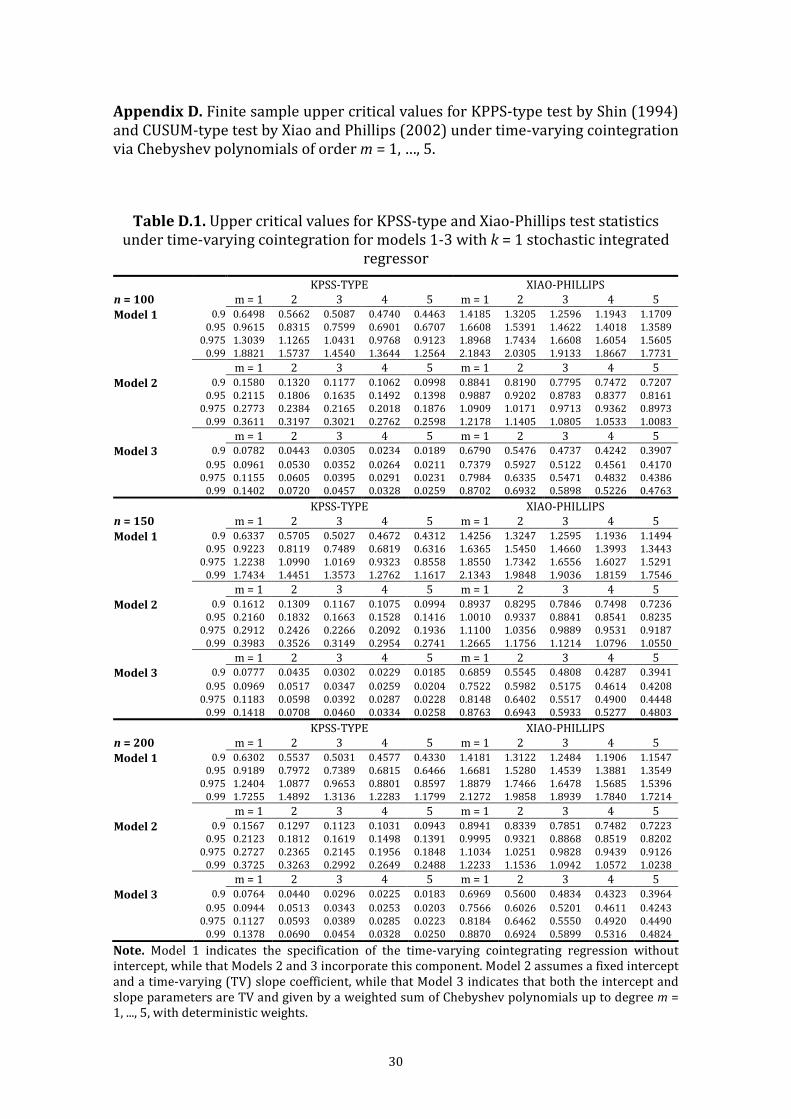
30
Appendix D. Finite sample upper critical values for KPPS-type test by Shin (1994)
and CUSUM-type test by Xiao and Phillips (2002) under time-varying cointegration
via Chebyshev polynomials of order m = 1, …, 5.
Table D.1. Upper critical values for KPSS-type and Xiao-Phillips test statistics
under time-varying cointegration for models 1-3 with k = 1 stochastic integrated
regressor
KPSS-TYPE XIAO-PHILLIPS
n = 100 m = 1 2 3 4 5 m = 1 2 3 4 5
0.9 0.6498 0.5662 0.5087 0.4740 0.4463 1.4185 1.3205 1.2596 1.1943 1.1709 Model 1 0.95 0.9615 0.8315 0.7599 0.6901 0.6707 1.6608 1.5391 1.4622 1.4018 1.3589
0.975 1.3039 1.1265 1.0431 0.9768 0.9123 1.8968 1.7434 1.6608 1.6054 1.5605
0.99 1.8821 1.5737 1.4540 1.3644 1.2564 2.1843 2.0305 1.9133 1.8667 1.7731
m = 1 2 3 4 5 m = 1 2 3 4 5
0.9 0.1580 0.1320 0.1177 0.1062 0.0998 0.8841 0.8190 0.7795 0.7472 0.7207 Model 2 0.95 0.2115 0.1806 0.1635 0.1492 0.1398 0.9887 0.9202 0.8783 0.8377 0.8161
0.975 0.2773 0.2384 0.2165 0.2018 0.1876 1.0909 1.0171 0.9713 0.9362 0.8973
0.99 0.3611 0.3197 0.3021 0.2762 0.2598 1.2178 1.1405 1.0805 1.0533 1.0083
m = 1 2 3 4 5 m = 1 2 3 4 5
0.9 0.0782 0.0443 0.0305 0.0234 0.0189 0.6790 0.5476 0.4737 0.4242 0.3907 Model 3 0.95 0.0961 0.0530 0.0352 0.0264 0.0211 0.7379 0.5927 0.5122 0.4561 0.4170
0.975 0.1155 0.0605 0.0395 0.0291 0.0231 0.7984 0.6335 0.5471 0.4832 0.4386
0.99 0.1402 0.0720 0.0457 0.0328 0.0259 0.8702 0.6932 0.5898 0.5226 0.4763
KPSS-TYPE XIAO-PHILLIPS
n = 150 m = 1 2 3 4 5 m = 1 2 3 4 5
0.9 0.6337 0.5705 0.5027 0.4672 0.4312 1.4256 1.3247 1.2595 1.1936 1.1494 Model 1 0.95 0.9223 0.8119 0.7489 0.6819 0.6316 1.6365 1.5450 1.4660 1.3993 1.3443
0.975 1.2238 1.0990 1.0169 0.9323 0.8558 1.8550 1.7342 1.6556 1.6027 1.5291
0.99 1.7434 1.4451 1.3573 1.2762 1.1617 2.1343 1.9848 1.9036 1.8159 1.7546
m = 1 2 3 4 5 m = 1 2 3 4 5
0.9 0.1612 0.1309 0.1167 0.1075 0.0994 0.8937 0.8295 0.7846 0.7498 0.7236 Model 2 0.95 0.2160 0.1832 0.1663 0.1528 0.1416 1.0010 0.9337 0.8841 0.8541 0.8235
0.975 0.2912 0.2426 0.2266 0.2092 0.1936 1.1100 1.0356 0.9889 0.9531 0.9187
0.99 0.3983 0.3526 0.3149 0.2954 0.2741 1.2665 1.1756 1.1214 1.0796 1.0550
m = 1 2 3 4 5 m = 1 2 3 4 5
0.9 0.0777 0.0435 0.0302 0.0229 0.0185 0.6859 0.5545 0.4808 0.4287 0.3941 Model 3 0.95 0.0969 0.0517 0.0347 0.0259 0.0204 0.7522 0.5982 0.5175 0.4614 0.4208
0.975 0.1183 0.0598 0.0392 0.0287 0.0228 0.8148 0.6402 0.5517 0.4900 0.4448
0.99 0.1418 0.0708 0.0460 0.0334 0.0258 0.8763 0.6943 0.5933 0.5277 0.4803
KPSS-TYPE XIAO-PHILLIPS
n = 200 m = 1 2 3 4 5 m = 1 2 3 4 5
0.9 0.6302 0.5537 0.5031 0.4577 0.4330 1.4181 1.3122 1.2484 1.1906 1.1547 Model 1 0.95 0.9189 0.7972 0.7389 0.6815 0.6466 1.6681 1.5280 1.4539 1.3881 1.3549
0.975 1.2404 1.0877 0.9653 0.8801 0.8597 1.8879 1.7466 1.6478 1.5685 1.5396
0.99 1.7255 1.4892 1.3136 1.2283 1.1799 2.1272 1.9858 1.8939 1.7840 1.7214
m = 1 2 3 4 5 m = 1 2 3 4 5
0.9 0.1567 0.1297 0.1123 0.1031 0.0943 0.8941 0.8339 0.7851 0.7482 0.7223 Model 2 0.95 0.2123 0.1812 0.1619 0.1498 0.1391 0.9995 0.9321 0.8868 0.8519 0.8202
0.975 0.2727 0.2365 0.2145 0.1956 0.1848 1.1034 1.0251 0.9828 0.9439 0.9126
0.99 0.3725 0.3263 0.2992 0.2649 0.2488 1.2233 1.1536 1.0942 1.0572 1.0238
m = 1 2 3 4 5 m = 1 2 3 4 5
0.9 0.0764 0.0440 0.0296 0.0225 0.0183 0.6969 0.5600 0.4834 0.4323 0.3964 Model 3 0.95 0.0944 0.0513 0.0343 0.0253 0.0203 0.7566 0.6026 0.5201 0.4611 0.4243
0.975 0.1127 0.0593 0.0389 0.0285 0.0223 0.8184 0.6462 0.5550 0.4920 0.4490
0.99 0.1378 0.0690 0.0454 0.0328 0.0250 0.8870 0.6924 0.5899 0.5316 0.4824
Note. Model 1 indicates the specification of the time-varying cointegrating regression without
intercept, while that Models 2 and 3 incorporate this component. Model 2 assumes a fixed intercept
and a time-varying (TV) slope coefficient, while that Model 3 indicates that both the intercept and
slope parameters are TV and given by a weighted sum of Chebyshev polynomials up to degree m =
1, ..., 5, with deterministic weights.
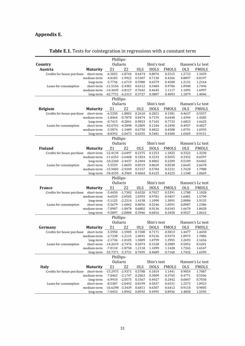
31
Appendix E.
Table E.1. Tests for cointegration in regressions with a constant term
Country
Phillips-
Ouliaris Shin’s test Hansen’s Lc test
Austria Maturity Z1 Z2 OLS DOLS FMOLS OLS FMOLS Credits for house purchase short-term -6.3825 -1.8744 0.6474 0.8076 0.5515 1.2723 1.3459
medium-term -4.8183 -1.9922 0.5307 0.7130 0.4266 0.8897 0.8197
long-term -5.7736 -1.6719 0.5980 0.6579 0.4508 1.2131 1.2164
Loans for consumption short-term -11.5156 -2.4381 0.6312 0.3484 0.9786 1.0940 1.7496
medium-term -14.3695 -2.8127 0.7642 0.4645 1.1117 1.1095 1.6997
long-term -62.7751 -6.2313 0.3727 0.3807 0.4093 1.1879 1.4046
Phillips-
Ouliaris Shin’s test Hansen’s Lc test
Belgium Maturity Z1 Z2 OLS DOLS FMOLS OLS FMOLS Credits for house purchase short-term -6.5250 -1.8802 0.2610 0.2821 0.1581 0.4637 0.5557
medium-term -1.8464 -0.7870 0.8474 0.7159 0.6448 1.4394 1.4585
long-term -0.7415 -0.2841 0.9833 0.7165 0.7733 1.6823 1.6625
Loans for consumption short-term -42.0701 -4.5898 0.2809 0.1244 0.2490 0.4957 0.4827
medium-term -5.5874 -1.3489 0.6750 0.4822 0.4588 1.0791 1.0393
long-term -8.8392 -2.0473 0.6555 0.5481 0.4300 1.0369 0.9151
Phillips-
Ouliaris Shin’s test Hansen’s Lc test
Finland Maturity Z1 Z2 OLS DOLS FMOLS OLS FMOLS Credits for house purchase short-term -12.4134 -2.6497 0.2375 0.1253 1.1825 0.3322 1.3230
medium-term -11.6353 -2.6468 0.1824 0.3233 0.5055 0.3352 0.6597
long-term -10.2260 -2.4437 0.2404 0.4065 0.2209 0.5109 0.6465
Loans for consumption short-term -5.5559 -1.8695 0.8519 0.8629 0.8538 2.6645 2.6678
medium-term -15.9483 -2.9349 0.5157 0.5784 0.5231 1.7620 1.7988
long-term -34.4559 -4.3969 0.4664 0.4125 0.4225 1.1348 1.0669
Phillips-
Ouliaris Shin’s test Hansen’s Lc test
France Maturity Z1 Z2 OLS DOLS FMOLS OLS FMOLS Credits for house purchase short-term -5.4450 -1.7302 0.6520 0.7027 0.5391 1.1780 1.1028
medium-term -4.6529 -2.0505 1.0393 0.9781 0.9457 1.6481 1.5790
long-term -5.1125 -2.2314 1.4138 1.1090 1.3091 2.0084 1.9135
Loans for consumption short-term -5.5679 -1.6842 0.8056 0.5246 1.0591 0.8987 1.2386
medium-term -7.0907 -1.8478 0.6802 0.9136 0.6343 1.6670 1.8428
long-term -9.5897 -2.0800 0.3946 0.6816 0.3458 0.9527 1.0616
Phillips-
Ouliaris Shin’s test Hansen’s Lc test
Germany Maturity Z1 Z2 OLS DOLS FMOLS OLS FMOLS Credits for house purchase short-term -5.5950 -1.5905 0.7208 0.7171 0.5813 1.4477 1.4430
medium-term -2.7338 -1.2115 1.0691 0.9136 0.9374 1.8975 1.7886
long-term -2.1736 -1.0105 1.5009 1.0799 1.3955 2.2693 2.1656
Loans for consumption short-term -14.2619 -2.7476 0.2074 0.1528 0.2089 0.5052 0.5201
medium-term -7.0110 -1.8758 1.2118 1.1099 1.1428 1.7265 1.6547
long-term -52.7371 -5.3731 0.7695 0.4689 0.7160 1.7432 1.6599
Phillips-
Ouliaris Shin’s test Hansen’s Lc test
Italy Maturity Z1 Z2 OLS DOLS FMOLS OLS FMOLS Credits for house purchase short-term -15.2975 -2.9371 0.5788 0.1819 1.1441 0.9054 1.7087
medium-term -7.0463 -2.1747 0.2863 0.3009 0.3765 0.4771 0.5506
long-term -6.9910 -2.0575 0.3367 0.4927 0.2442 0.6847 0.7030
Loans for consumption short-term -8.5387 -2.0492 0.8199 0.5037 0.6531 1.2573 1.0923
medium-term -16.6298 -3.3439 0.6811 0.6507 0.6412 0.9118 0.9005
long-term -7.0453 -1.8942 0.8592 0.4995 0.8936 1.4858 1.5595

32
Table E.1. Tests for cointegration in regressions with a constant term
(continuation)
Phillips-
Ouliaris Shin’s test Hansen’s Lc test
Spain Maturity Z1 Z2 OLS DOLS FMOLS OLS FMOLS Credits for house purchase short-term -6.7332 -1.7731 0.5407 0.2375 0.5347 1.2117 1.2156
medium-term -4.8093 -1.4928 0.9160 0.4588 1.0536 1.6208 1.8573
long-term -5.4733 -1.6119 0.2969 0.2524 0.3798 0.5227 0.6040
Loans for consumption short-term -20.6012 -3.3605 0.2926 0.2420 0.3502 0.5322 0.5429
medium-term -10.0494 -2.2883 0.9345 0.6010 0.9406 2.0250 2.0797
long-term -5.0576 -1.5845 1.0582 0.7020 1.1811 1.5742 1.8131
Notes. Asymptotic critical values for Z1 (normalized estimation error) and Z2 (pseudo-T ratio) test
statistics by Phillips and Ouliaris (1990)are given by −17.0309(10%), −20.4935(5%),
−28.3218(1%), and −3.0657(10%), −3.3654(5%), −3.9618(1%), respectively. For the Shin’s test,
the critical values are 0.231(10%), 0.314(5%) and 0.533(1%), while that for Hansen’s test for
stability of the cointegration relationship are 0.450(10%), 0.575(%), and 0.898(1%).

33
Table E.2. Tests for cointegration in time-varying regressions with a constant term
Country Credits for house purchase Loans for consumption
Austria Model 2. Fixed intercept, TV slope Model 3. TV intercept and slope Model 2. Fixed intercept, TV slope Model 3. TV intercept and slope
Maturity TV-KPSS TV-XP HQC TV-KPSS TV-XP HQC TV-KPSS TV-XP HQC TV-KPSS TV-XP HQC
short m = 1 0.4714 1.1253 -199.4073 0.1661 0.8553 -315.0593 0.5982 1.5331 -428.8247 0.1488 0.8408 -512.7211
2 0.4187 1.3210 -219.7468 0.1511 0.7029 -318.9892 0.2426 1.1130 -543.3924 0.0930 0.5944 -588.1555
3 0.4427 1.2556 -307.9701 0.0577 0.5681 -457.8922 0.1794 0.8826 -574.1671 0.0695 0.4640 -623.7697
4 0.2579 1.0620 -323.9294 0.0429 0.4603 -522.4725 0.2413 1.1299 -592.5537 0.0274 0.3594 -672.9680
5 0.2603 1.0481 -321.0162 0.0287 0.4339 -606.4163 0.0910 0.7109 -637.8969 0.0215 0.3707 -687.7957
6 0.2504 1.0276 -321.0191 0.0204 0.3594 -633.7684 0.0617 0.5713 -653.3452 0.0196 0.3860 -705.2680
7 0.2675 1.0395 -319.6615 0.0162 0.3532 -689.6035 0.0610 0.5489 -650.9108 0.0194 0.4105 -702.9163
8 0.2431 0.9949 -341.7791 0.0152 0.3594 -698.0421 0.0645 0.5412 -648.1755 0.0158 0.2822 -758.7472
9 0.2088 1.0207 -348.7296 0.0131 0.3365 -712.7086 0.0653 0.5971 -649.6654 0.0148 0.3881 -779.0521
10 0.2186 0.8912 -372.7239 0.0130 0.4262 -747.0597 0.0884 0.7714 -665.0045 0.0115 0.3145 -828.7065
medium m = 1 0.3429 0.9926 -130.0929 0.1927 0.8982 -176.9936 0.6630 1.6355 -207.8961 0.2052 0.9938 -303.4787
2 0.2953 1.1440 -139.4117 0.1833 0.7998 -176.4340 0.2364 0.9140 -329.4380 0.1179 0.6670 -359.4704
3 0.2600 1.1577 -317.4774 0.0660 0.5327 -394.6232 0.1316 0.7090 -381.3519 0.0833 0.5821 -406.1717
4 0.2743 1.1749 -314.3871 0.0510 0.4892 -612.9785 0.1889 0.9660 -406.6288 0.0290 0.4985 -472.5316
5 0.2732 1.1989 -311.7992 0.0255 0.4353 -799.7428 0.0316 0.4060 -464.1432 0.0239 0.4662 -481.5911
6 0.2620 1.1899 -325.6590 0.0238 0.3770 -810.2076 0.0298 0.4610 -463.0120 0.0153 0.3804 -500.6645
7 0.2575 1.1878 -322.6613 0.0165 0.4002 -900.3232 0.0274 0.4496 -461.2465 0.0148 0.3760 -497.9047
8 0.2304 1.1461 -341.0587 0.0136 0.3409 -963.3521 0.0291 0.4419 -459.5987 0.0129 0.3475 -507.3670
9 0.2095 1.1379 -340.7092 0.0124 0.4114 -976.6048 0.0298 0.3861 -469.3075 0.0127 0.3628 -508.7950
10 0.2250 1.0511 -369.0754 0.0116 0.4130 -998.8054 0.0337 0.4759 -477.0555 0.0129 0.3423 -508.8845
long m = 1 0.4831 1.1962 -196.9633 0.1413 0.6394 -320.9471 0.3862 1.3488 -310.9482 0.2614 0.9080 -327.6337
2 0.4418 1.3392 -203.3915 0.1416 0.6369 -320.0035 0.1575 1.0023 -376.4537 0.0998 0.7131 -392.4416
3 0.4475 1.2610 -271.2300 0.0588 0.5744 -429.1816 0.1934 1.0222 -389.8812 0.0584 0.5833 -429.6534
4 0.2623 1.0670 -287.9771 0.0459 0.4899 -499.4448 0.1260 0.9426 -403.8452 0.0214 0.3785 -457.2409
5 0.2635 1.0574 -284.8872 0.0367 0.4133 -585.9552 0.1425 1.0077 -400.9084 0.0193 0.3846 -458.7094
6 0.2563 1.0427 -282.9009 0.0257 0.3260 -635.7287 0.1200 0.9389 -405.9302 0.0192 0.4155 -457.8686
7 0.2693 1.0497 -280.8947 0.0159 0.3155 -782.6227 0.1204 0.9284 -403.1564 0.0160 0.3863 -462.6698
8 0.2453 1.0095 -306.3026 0.0154 0.2859 -780.9741 0.1035 0.8957 -403.5228 0.0127 0.3716 -468.1772
9 0.2099 1.0468 -314.6846 0.0126 0.3090 -805.3293 0.1135 0.9329 -404.9907 0.0107 0.2931 -478.1957
10 0.2303 0.9351 -348.6441 0.0118 0.3785 -851.1246 0.1114 0.9243 -402.3490 0.0106 0.3163 -480.1331
Note. HQC is the estimated value of the Hannan-Quinn information criterion defined by HQC(n,k,m) = nlog(SSR(k,m)/n) + 2(k+1)(m+1)log(log(n)), with k = 1. The
critical values for testing the null of time-varying cointegration for each model and test statistic (TV-KPSS and TV-XP) are given in Table D.1
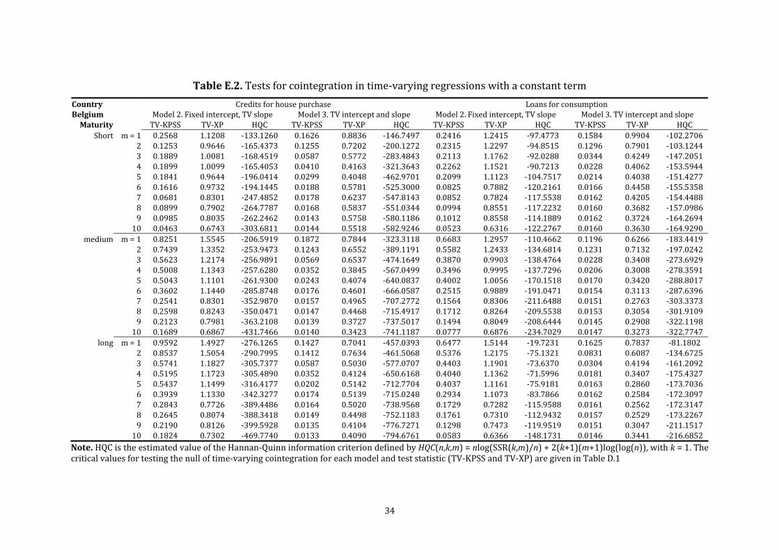
34
Table E.2. Tests for cointegration in time-varying regressions with a constant term
Country Credits for house purchase Loans for consumption
Belgium Model 2. Fixed intercept, TV slope Model 3. TV intercept and slope Model 2. Fixed intercept, TV slope Model 3. TV intercept and slope
Maturity TV-KPSS TV-XP HQC TV-KPSS TV-XP HQC TV-KPSS TV-XP HQC TV-KPSS TV-XP HQC
Short m = 1 0.2568 1.1208 -133.1260 0.1626 0.8836 -146.7497 0.2416 1.2415 -97.4773 0.1584 0.9904 -102.2706
2 0.1253 0.9646 -165.4373 0.1255 0.7202 -200.1272 0.2315 1.2297 -94.8515 0.1296 0.7901 -103.1244
3 0.1889 1.0081 -168.4519 0.0587 0.5772 -283.4843 0.2113 1.1762 -92.0288 0.0344 0.4249 -147.2051
4 0.1899 1.0099 -165.4053 0.0410 0.4163 -321.3643 0.2262 1.1521 -90.7213 0.0228 0.4062 -153.5944
5 0.1841 0.9644 -196.0414 0.0299 0.4048 -462.9701 0.2099 1.1123 -104.7517 0.0214 0.4038 -151.4277
6 0.1616 0.9732 -194.1445 0.0188 0.5781 -525.3000 0.0825 0.7882 -120.2161 0.0166 0.4458 -155.5358
7 0.0681 0.8301 -247.4852 0.0178 0.6237 -547.8143 0.0852 0.7824 -117.5538 0.0162 0.4205 -154.4488
8 0.0899 0.7902 -264.7787 0.0168 0.5837 -551.0344 0.0994 0.8551 -117.2232 0.0160 0.3682 -157.0986
9 0.0985 0.8035 -262.2462 0.0143 0.5758 -580.1186 0.1012 0.8558 -114.1889 0.0162 0.3724 -164.2694
10 0.0463 0.6743 -303.6811 0.0144 0.5518 -582.9246 0.0523 0.6316 -122.2767 0.0160 0.3630 -164.9290
medium m = 1 0.8251 1.5545 -206.5919 0.1872 0.7844 -323.3118 0.6683 1.2957 -110.4662 0.1196 0.6266 -183.4419
2 0.7439 1.3352 -253.9473 0.1243 0.6552 -389.1191 0.5582 1.2433 -134.6814 0.1231 0.7132 -197.0242
3 0.5623 1.2174 -256.9891 0.0569 0.6537 -474.1649 0.3870 0.9903 -138.4764 0.0228 0.3408 -273.6929
4 0.5008 1.1343 -257.6280 0.0352 0.3845 -567.0499 0.3496 0.9995 -137.7296 0.0206 0.3008 -278.3591
5 0.5043 1.1101 -261.9300 0.0243 0.4074 -640.0837 0.4002 1.0056 -170.1518 0.0170 0.3420 -288.8017
6 0.3602 1.1440 -285.8748 0.0176 0.4601 -666.0587 0.2515 0.9889 -191.0471 0.0154 0.3113 -287.6396
7 0.2541 0.8301 -352.9870 0.0157 0.4965 -707.2772 0.1564 0.8306 -211.6488 0.0151 0.2763 -303.3373
8 0.2598 0.8243 -350.0471 0.0147 0.4468 -715.4917 0.1712 0.8264 -209.5538 0.0153 0.3054 -301.9109
9 0.2123 0.7981 -363.2108 0.0139 0.3727 -737.5017 0.1494 0.8049 -208.6444 0.0145 0.2908 -322.1198
10 0.1689 0.6867 -431.7466 0.0140 0.3423 -741.1187 0.0777 0.6876 -234.7029 0.0147 0.3273 -322.7747
long m = 1 0.9592 1.4927 -276.1265 0.1427 0.7041 -457.0393 0.6477 1.5144 -19.7231 0.1625 0.7837 -81.1802
2 0.8537 1.5054 -290.7995 0.1412 0.7634 -461.5068 0.5376 1.2175 -75.1321 0.0831 0.6087 -134.6725
3 0.5741 1.1827 -305.7377 0.0587 0.5030 -577.0707 0.4403 1.1901 -73.6370 0.0304 0.4194 -161.2092
4 0.5195 1.1723 -305.4890 0.0352 0.4124 -650.6168 0.4040 1.1362 -71.5996 0.0181 0.3407 -175.4327
5 0.5437 1.1499 -316.4177 0.0202 0.5142 -712.7704 0.4037 1.1161 -75.9181 0.0163 0.2860 -173.7036
6 0.3939 1.1330 -342.3277 0.0174 0.5139 -715.0248 0.2934 1.1073 -83.7866 0.0162 0.2584 -172.3097
7 0.2843 0.7726 -389.4486 0.0164 0.5020 -738.9568 0.1729 0.7282 -115.9588 0.0161 0.2562 -172.3147
8 0.2645 0.8074 -388.3418 0.0149 0.4498 -752.1183 0.1761 0.7310 -112.9432 0.0157 0.2529 -173.2267
9 0.2190 0.8126 -399.5928 0.0135 0.4104 -776.7271 0.1298 0.7473 -119.9519 0.0151 0.3047 -211.1517
10 0.1824 0.7302 -469.7740 0.0133 0.4090 -794.6761 0.0583 0.6366 -148.1731 0.0146 0.3441 -216.6852
Note. HQC is the estimated value of the Hannan-Quinn information criterion defined by HQC(n,k,m) = nlog(SSR(k,m)/n) + 2(k+1)(m+1)log(log(n)), with k = 1. The
critical values for testing the null of time-varying cointegration for each model and test statistic (TV-KPSS and TV-XP) are given in Table D.1

35
Table E.2. Tests for cointegration in time-varying regressions with a constant term
Country Credits for house purchase Loans for consumption
Finland Model 2. Fixed intercept, TV slope Model 3. TV intercept and slope Model 2. Fixed intercept, TV slope Model 3. TV intercept and slope
Maturity TV-KPSS TV-XP HQC TV-KPSS TV-XP HQC TV-KPSS TV-XP HQC TV-KPSS TV-XP HQC
Short m = 1 0.1517 0.6966 -399.6078 0.1429 0.6844 -403.5275 0.6413 1.3403 -274.8459 0.1640 0.9684 -362.1959
2 0.1337 0.7013 -401.9850 0.1296 0.6012 -406.9145 0.3584 1.3990 -345.0941 0.0669 0.5309 -495.7892
3 0.0681 0.6524 -492.9469 0.0499 0.5811 -520.2213 0.3085 1.2211 -362.4214 0.0378 0.6685 -540.4210
4 0.0509 0.7058 -500.4465 0.0371 0.4469 -543.0967 0.3321 1.2756 -361.2184 0.0285 0.5554 -546.6198
5 0.0481 0.6469 -501.4704 0.0253 0.3897 -596.9699 0.1783 0.8125 -412.2612 0.0253 0.4716 -553.2159
6 0.0453 0.6447 -503.3490 0.0196 0.3816 -611.3773 0.1347 0.8311 -448.9335 0.0243 0.4470 -557.5370
7 0.0537 0.6834 -533.0356 0.0161 0.3296 -672.1877 0.1448 0.8075 -466.3018 0.0155 0.3323 -603.9686
8 0.0490 0.6448 -570.7725 0.0142 0.3129 -697.3619 0.1329 0.7760 -465.2405 0.0154 0.3432 -601.8057
9 0.0477 0.6417 -567.9272 0.0128 0.3168 -707.5506 0.1333 0.7757 -461.9653 0.0142 0.2984 -613.9475
10 0.0251 0.5240 -631.5737 0.0122 0.5473 -765.5951 0.1395 0.8041 -459.9964 0.0110 0.2630 -637.6453
medium m = 1 0.2130 0.7402 -370.3123 0.1414 0.7373 -390.2133 0.5233 1.3420 35.9286 0.0929 0.7886 -39.5770
2 0.1656 0.8403 -382.6126 0.1237 0.5883 -394.6929 0.2519 1.2992 -7.7112 0.0609 0.9892 -64.3032
3 0.0608 0.6908 -475.7831 0.0492 0.6106 -494.9389 0.2097 1.2392 -13.9615 0.0626 0.9954 -63.3177
4 0.0767 0.7369 -473.7631 0.0388 0.4683 -520.8632 0.1928 1.1860 -11.9993 0.0531 0.8709 -70.6154
5 0.0782 0.7099 -471.2626 0.0314 0.4350 -562.7376 0.0913 0.7901 -36.9571 0.0368 0.7500 -94.1883
6 0.0746 0.7046 -469.6810 0.0229 0.3506 -596.1270 0.0845 0.7965 -36.3828 0.0244 0.6429 -147.0704
7 0.1061 0.7443 -494.9428 0.0163 0.3253 -719.7410 0.0846 0.7646 -37.5754 0.0215 0.5890 -174.0815
8 0.0861 0.7138 -533.8477 0.0147 0.2956 -737.2003 0.0625 0.7603 -55.9874 0.0172 0.5535 -199.2611
9 0.0806 0.7269 -532.0614 0.0133 0.3007 -748.3447 0.0558 0.7361 -81.2319 0.0150 0.6051 -223.2643
10 0.0702 0.6319 -612.1995 0.0127 0.5461 -827.4028 0.0579 0.6795 -88.7836 0.0125 0.6137 -246.1418
long m = 1 0.2815 0.8457 -304.2661 0.1242 0.6529 -345.4383 0.4812 1.5381 185.4967 0.1173 0.8749 126.3500
2 0.2336 0.9789 -313.5978 0.1145 0.5677 -345.5378 0.2365 1.2598 143.3876 0.0948 0.8646 104.9462
3 0.1584 0.8312 -390.9413 0.0574 0.6242 -427.4373 0.2517 1.3006 146.0306 0.0743 0.8773 96.8749
4 0.1250 0.7882 -389.1363 0.0433 0.4508 -461.8645 0.1887 1.2486 133.0501 0.0330 0.6060 46.1198
5 0.1254 0.7840 -385.9457 0.0351 0.4290 -533.1887 0.1042 0.9268 122.1609 0.0186 0.4065 27.7893
6 0.1228 0.7780 -383.2757 0.0254 0.3332 -572.9655 0.1011 0.8686 123.2786 0.0145 0.5146 20.3037
7 0.1663 0.8256 -403.4467 0.0162 0.3046 -769.0209 0.1005 0.8965 121.6133 0.0137 0.5323 21.6434
8 0.1443 0.8105 -450.2007 0.0150 0.2918 -784.4111 0.0717 0.7526 107.5369 0.0143 0.5445 20.8311
9 0.1203 0.8546 -455.0972 0.0136 0.2828 -792.8693 0.0691 0.7612 106.3521 0.0146 0.5569 22.7175
10 0.1318 0.7597 -513.7703 0.0128 0.4988 -883.4579 0.0732 0.8400 103.5313 0.0138 0.5409 20.9499
Note. HQC is the estimated value of the Hannan-Quinn information criterion defined by HQC(n,k,m) = nlog(SSR(k,m)/n) + 2(k+1)(m+1)log(log(n)), with k = 1. The
critical values for testing the null of time-varying cointegration for each model and test statistic (TV-KPSS and TV-XP) are given in Table D.1

36
Table E.2. Tests for cointegration in time-varying regressions with a constant term
Country Credits for house purchase Loans for consumption
France Model 2. Fixed intercept, TV slope Model 3. TV intercept and slope Model 2. Fixed intercept, TV slope Model 3. TV intercept and slope
Maturity TV-KPSS TV-XP HQC TV-KPSS TV-XP HQC TV-KPSS TV-XP HQC TV-KPSS TV-XP HQC
Short m = 1 0.4402 1.0069 -238.0710 0.1946 0.9422 -306.6659 0.5387 1.5423 -80.1440 0.2608 0.9036 -146.9802
2 0.3718 1.2077 -259.8456 0.1654 0.7971 -320.8163 0.1907 1.0538 -161.9495 0.1321 0.6989 -201.6628
3 0.3834 1.1803 -364.6054 0.0562 0.5329 -476.7271 0.1399 0.6469 -271.8893 0.0918 0.5552 -336.7957
4 0.3099 1.0596 -363.8852 0.0386 0.4355 -553.3542 0.0970 0.8505 -305.3118 0.0379 0.4576 -417.0800
5 0.3111 1.0307 -370.0457 0.0275 0.4379 -603.2606 0.1551 0.8469 -324.1537 0.0278 0.4176 -459.8406
6 0.3017 1.0245 -369.6747 0.0194 0.3697 -616.0507 0.1151 0.7389 -353.4380 0.0239 0.3870 -485.7253
7 0.2896 1.0391 -369.2190 0.0122 0.2992 -640.6168 0.1162 0.7449 -352.6902 0.0227 0.4021 -493.3991
8 0.2837 0.9999 -417.5418 0.0121 0.3077 -637.4841 0.0957 0.7588 -368.2403 0.0122 0.3260 -550.4998
9 0.2329 1.0261 -436.1980 0.0118 0.2984 -636.3234 0.0985 0.7547 -366.0114 0.0097 0.3381 -562.0219
10 0.2354 0.9320 -441.6805 0.0110 0.2589 -641.2921 0.1032 0.7688 -426.9554 0.0094 0.2919 -567.0266
medium m = 1 0.4746 1.0806 -242.6087 0.2233 1.1196 -334.5960 0.2424 0.9821 -328.0875 0.2404 0.9644 -328.1142
2 0.4059 1.3077 -287.1995 0.1776 0.8614 -364.2656 0.2751 0.9562 -391.8681 0.0894 0.5091 -440.1651
3 0.4902 1.3246 -417.3118 0.0630 0.5069 -573.8839 0.2683 0.9583 -388.6569 0.0715 0.5633 -475.2030
4 0.3484 1.1054 -422.9995 0.0480 0.4310 -701.8762 0.1688 0.9381 -441.9564 0.0585 0.5964 -492.0719
5 0.3483 1.1487 -423.5605 0.0232 0.3319 -771.9683 0.1837 0.9747 -438.9337 0.0394 0.4496 -587.8502
6 0.3373 1.1130 -424.5375 0.0189 0.3308 -771.3876 0.1917 1.0306 -437.0485 0.0286 0.4247 -643.9389
7 0.3288 1.1075 -422.0236 0.0131 0.4121 -786.7734 0.1887 0.9985 -437.1250 0.0176 0.3257 -693.1846
8 0.3078 1.0781 -450.8141 0.0131 0.3550 -785.2585 0.2000 0.9986 -435.0887 0.0151 0.3502 -695.1711
9 0.2604 1.0967 -464.6948 0.0130 0.3744 -783.8521 0.2185 0.9963 -444.6288 0.0123 0.2962 -711.1100
10 0.2586 1.0182 -467.6460 0.0130 0.3712 -781.6353 0.2277 0.9756 -460.0425 0.0119 0.2829 -710.0984
long m = 1 0.5046 1.1686 -340.4669 0.2327 1.1265 -452.2350 0.1994 0.8371 -303.3133 0.2020 0.9055 -303.7111
2 0.4512 1.3563 -403.6018 0.1640 0.8105 -503.3346 0.2529 0.9771 -344.6633 0.0717 0.5293 -391.8941
3 0.5681 1.4050 -508.6121 0.0612 0.5072 -677.7499 0.2452 0.9814 -341.4875 0.0672 0.5406 -403.7179
4 0.3478 1.1040 -527.4378 0.0405 0.4275 -742.6834 0.1620 0.9567 -380.9035 0.0525 0.5553 -426.9200
5 0.3459 1.0851 -524.6387 0.0179 0.3875 -776.7483 0.1358 0.8918 -378.8631 0.0356 0.3828 -503.9608
6 0.3388 1.0968 -522.4715 0.0194 0.3881 -775.3036 0.1579 1.0472 -385.3209 0.0278 0.4123 -562.8369
7 0.3352 1.0973 -519.3562 0.0165 0.4988 -782.2095 0.1561 1.0197 -384.5309 0.0150 0.2897 -651.7362
8 0.3068 1.0214 -535.6892 0.0159 0.4371 -781.5165 0.1748 1.0240 -386.0044 0.0112 0.2276 -664.6872
9 0.2591 1.0130 -557.6636 0.0157 0.4369 -779.0287 0.1805 1.0097 -386.8335 0.0091 0.2597 -679.5562
10 0.2556 0.9513 -556.7372 0.0160 0.4139 -777.1447 0.1957 1.0193 -425.8239 0.0091 0.2573 -691.5234
Note. HQC is the estimated value of the Hannan-Quinn information criterion defined by HQC(n,k,m) = nlog(SSR(k,m)/n) + 2(k+1)(m+1)log(log(n)), with k = 1. The
critical values for testing the null of time-varying cointegration for each model and test statistic (TV-KPSS and TV-XP) are given in Table D.1

37
Table E.2. Tests for cointegration in time-varying regressions with a constant term
Country Credits for house purchase Loans for consumption
Germany Model 2. Fixed intercept, TV slope Model 3. TV intercept and slope Model 2. Fixed intercept, TV slope Model 3. TV intercept and slope
Maturity TV-KPSS TV-XP HQC TV-KPSS TV-XP HQC TV-KPSS TV-XP HQC TV-KPSS TV-XP HQC
Short m = 1 0.5406 1.2599 -263.0508 0.1431 0.7109 -410.2262 0.1986 1.1860 -157.0713 0.1986 1.1868 -157.0714
2 0.4948 1.4051 -273.4850 0.1355 0.6748 -415.4084 0.2416 1.2818 -181.9103 0.1098 0.8064 -225.2593
3 0.5142 1.3665 -329.6471 0.0587 0.6398 -513.0534 0.1847 1.1414 -209.8967 0.0796 0.6092 -269.1327
4 0.2900 1.0507 -356.4809 0.0433 0.5261 -561.9621 0.2188 1.2595 -218.1050 0.0366 0.5718 -349.9416
5 0.2889 1.0576 -353.3472 0.0279 0.4212 -653.8802 0.1054 0.9707 -272.3718 0.0265 0.5685 -404.5317
6 0.2804 1.0353 -352.1798 0.0167 0.3238 -718.1553 0.0621 0.8284 -310.3117 0.0235 0.5139 -405.7443
7 0.3028 1.0586 -351.5423 0.0143 0.3423 -742.7004 0.0550 0.7897 -318.5761 0.0231 0.4735 -406.7572
8 0.2880 1.0396 -387.9432 0.0138 0.2944 -758.5945 0.0570 0.7934 -319.3635 0.0147 0.2861 -474.4178
9 0.2453 1.0527 -399.2545 0.0129 0.3093 -762.1545 0.0568 0.7975 -316.1274 0.0104 0.3383 -494.9066
10 0.2459 0.9488 -408.3747 0.0122 0.2939 -807.5219 0.0513 0.7476 -321.4031 0.0106 0.3082 -496.0923
medium m = 1 0.6064 1.3791 -246.9386 0.2111 0.9679 -417.3691 0.4224 1.2874 -386.4556 0.1493 0.7955 -454.6440
2 0.5609 1.5185 -278.3636 0.1685 0.8005 -459.6959 0.4165 1.2819 -383.1754 0.0933 0.6120 -524.5963
3 0.6280 1.4837 -344.7926 0.0667 0.5286 -717.9006 0.2323 1.0083 -501.8537 0.0420 0.5588 -578.5874
4 0.3772 1.1484 -385.8735 0.0452 0.4078 -851.5763 0.1245 0.7393 -551.5789 0.0238 0.5145 -617.7367
5 0.3770 1.1530 -386.6826 0.0201 0.4257 -1005.7446 0.0760 0.6731 -553.5919 0.0247 0.5388 -621.4684
6 0.3648 1.1330 -388.3252 0.0185 0.3497 -1007.6578 0.0772 0.5650 -553.7348 0.0173 0.5599 -638.2931
7 0.3559 1.1323 -385.9008 0.0166 0.3409 -1050.8041 0.0643 0.4902 -573.8952 0.0160 0.5384 -641.4065
8 0.3302 1.0605 -407.6466 0.0152 0.3412 -1076.5100 0.0741 0.5243 -573.7967 0.0144 0.5217 -650.1784
9 0.2834 1.0852 -442.6575 0.0133 0.2789 -1098.4979 0.0765 0.5195 -575.0008 0.0125 0.4692 -662.9848
10 0.2801 1.0149 -443.4316 0.0126 0.4046 -1190.6930 0.0843 0.6097 -578.3956 0.0124 0.4633 -673.0394
long m = 1 0.6778 1.5454 -329.2332 0.2253 0.8458 -634.6166 0.7581 1.3597 -399.8182 0.1074 0.6192 -496.9619
2 0.6606 1.5516 -368.0696 0.1315 0.6893 -727.6561 0.4860 1.4678 -427.0635 0.0620 0.5042 -516.0585
3 0.6626 1.4808 -387.8647 0.0851 0.6663 -910.6462 0.3818 1.3811 -466.3692 0.0269 0.5292 -541.3408
4 0.3733 1.1275 -466.2976 0.0465 0.5319 -1057.0795 0.3343 1.2730 -469.0670 0.0226 0.5561 -541.6830
5 0.3729 1.1241 -463.1076 0.0317 0.4507 -1146.8539 0.1573 0.8132 -497.0725 0.0233 0.5459 -538.9567
6 0.3737 1.1240 -459.9071 0.0196 0.3657 -1237.7063 0.1359 0.8253 -497.5209 0.0223 0.5083 -539.5657
7 0.3597 1.1316 -459.3527 0.0179 0.3381 -1268.5282 0.1381 0.8054 -495.0973 0.0149 0.4445 -551.0601
8 0.3299 1.0554 -477.4433 0.0165 0.3566 -1279.2273 0.1245 0.7252 -495.0609 0.0126 0.4939 -552.9516
9 0.2804 1.0342 -510.3423 0.0149 0.3396 -1293.8650 0.1282 0.8212 -499.3882 0.0119 0.4567 -553.3320
10 0.2780 1.0103 -507.4669 0.0151 0.4449 -1360.4082 0.1229 0.7756 -503.4376 0.0105 0.3985 -557.7708
Note. HQC is the estimated value of the Hannan-Quinn information criterion defined by HQC(n,k,m) = nlog(SSR(k,m)/n) + 2(k+1)(m+1)log(log(n)), with k = 1. The
critical values for testing the null of time-varying cointegration for each model and test statistic (TV-KPSS and TV-XP) are given in Table D.1

38
Table E.2. Tests for cointegration in time-varying regressions with a constant term
Country Credits for house purchase Loans for consumption
Italy Model 2. Fixed intercept, TV slope Model 3. TV intercept and slope Model 2. Fixed intercept, TV slope Model 3. TV intercept and slope
Maturity TV-KPSS TV-XP HQC TV-KPSS TV-XP HQC TV-KPSS TV-XP HQC TV-KPSS TV-XP HQC
Short m = 1 0.2802 0.9778 -194.5226 0.1595 0.7701 -215.0331 0.4067 1.5528 42.5701 0.1610 1.0974 -37.0996
2 0.3025 1.1184 -196.0750 0.1153 0.6826 -240.4917 0.4678 1.5089 37.2301 0.0999 0.8245 -115.2457
3 0.3830 1.3485 -212.7152 0.0481 0.5565 -306.6385 0.4470 1.3977 12.0736 0.0464 0.6361 -157.3353
4 0.1041 0.7016 -288.5038 0.0370 0.4794 -338.0063 0.2389 1.2799 -10.3322 0.0293 0.5061 -207.7046
5 0.0982 0.6891 -286.4423 0.0271 0.5148 -375.0906 0.2657 1.2473 -21.7182 0.0228 0.5080 -222.6727
6 0.0990 0.7002 -283.2679 0.0207 0.3987 -386.5916 0.2561 1.2278 -20.3237 0.0193 0.4783 -253.6854
7 0.0836 0.7169 -305.7507 0.0134 0.5225 -413.6370 0.2547 1.2270 -17.1350 0.0141 0.4010 -281.0538
8 0.0872 0.7345 -302.7312 0.0134 0.5198 -410.6964 0.2272 1.1926 -35.7853 0.0141 0.4110 -280.3427
9 0.0600 0.5954 -305.8175 0.0131 0.5623 -411.9126 0.2072 1.1843 -34.5542 0.0141 0.3758 -285.5941
10 0.0684 0.6535 -324.5373 0.0123 0.5288 -416.7729 0.2074 1.0959 -44.7271 0.0134 0.4028 -304.9342
medium m = 1 0.2960 0.8668 -339.5221 0.1721 0.8181 -366.1071 0.1522 0.6891 -223.0528 0.1188 0.5970 -229.5852
2 0.2584 0.9701 -344.8618 0.1640 0.7285 -371.7882 0.1059 0.7447 -232.6272 0.0948 0.5807 -234.7863
3 0.1786 0.8178 -480.9173 0.0539 0.5111 -571.6701 0.0710 0.6136 -259.7445 0.0674 0.5328 -261.1392
4 0.1879 0.8452 -477.8016 0.0422 0.4699 -623.0589 0.0879 0.7749 -260.8696 0.0439 0.4577 -290.6180
5 0.1774 0.8767 -485.6871 0.0312 0.4510 -703.6536 0.0897 0.8024 -258.0814 0.0257 0.5479 -364.8322
6 0.1631 0.8866 -505.2286 0.0242 0.3436 -741.0667 0.0911 0.7844 -256.0464 0.0180 0.5188 -396.2947
7 0.1955 0.9088 -511.4706 0.0189 0.3440 -845.2505 0.1182 0.7981 -283.7627 0.0146 0.4468 -405.5350
8 0.1705 0.8597 -532.2535 0.0162 0.3623 -859.3016 0.0800 0.7534 -319.3018 0.0125 0.4617 -420.1216
9 0.1429 0.8926 -537.5601 0.0139 0.4285 -877.5955 0.0734 0.7468 -316.3463 0.0122 0.4348 -428.4904
10 0.1472 0.7661 -578.6857 0.0145 0.5867 -898.5156 0.0736 0.7317 -315.0783 0.0118 0.4273 -429.8371
long m = 1 0.3606 0.9876 -323.9181 0.1692 0.8378 -375.2126 0.4759 1.5996 -171.4382 0.1618 0.8439 -267.2800
2 0.3134 1.1514 -333.5626 0.1603 0.7388 -378.8605 0.4860 1.6289 -168.6964 0.0930 0.7485 -314.3514
3 0.2689 0.9922 -448.2277 0.0574 0.5334 -533.4669 0.4686 1.6176 -167.1982 0.0786 0.6142 -322.2929
4 0.2331 0.9330 -445.8383 0.0437 0.4897 -606.2877 0.2081 1.1244 -237.2550 0.0421 0.4321 -403.5871
5 0.2280 0.9911 -445.9371 0.0292 0.4107 -705.5798 0.2075 1.1093 -235.2090 0.0258 0.4004 -471.9399
6 0.2160 0.9712 -453.6742 0.0215 0.3740 -742.6775 0.1885 1.0532 -250.8479 0.0153 0.3124 -492.4075
7 0.2437 0.9954 -455.5953 0.0166 0.3093 -815.1000 0.1718 0.9789 -295.0498 0.0132 0.3630 -506.2128
8 0.2217 0.9545 -485.3006 0.0152 0.3141 -832.2697 0.1851 1.0190 -292.8965 0.0128 0.3778 -504.3291
9 0.1907 0.9750 -490.9297 0.0137 0.3187 -846.1873 0.1628 0.9712 -293.8814 0.0124 0.3394 -504.4999
10 0.2102 0.8525 -530.6802 0.0130 0.3507 -965.1140 0.1569 0.9246 -301.7068 0.0121 0.3340 -502.7054
Note. HQC is the estimated value of the Hannan-Quinn information criterion defined by HQC(n,k,m) = nlog(SSR(k,m)/n) + 2(k+1)(m+1)log(log(n)), with k = 1. The
critical values for testing the null of time-varying cointegration for each model and test statistic (TV-KPSS and TV-XP) are given in Table D.1
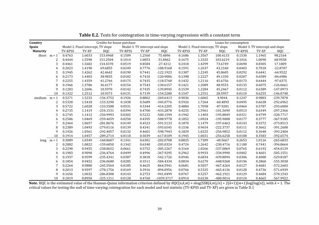
39
Table E.2. Tests for cointegration in time-varying regressions with a constant term
Country Credits for house purchase Loans for consumption
Spain Model 2. Fixed intercept, TV slope Model 3. TV intercept and slope Model 2. Fixed intercept, TV slope Model 3. TV intercept and slope
Maturity TV-KPSS TV-XP HQC TV-KPSS TV-XP HQC TV-KPSS TV-XP HQC TV-KPSS TV-XP HQC
Short m = 1 0.4763 1.6033 153.4968 0.1509 1.2560 75.4896 0.1686 1.3567 100.4133 0.1530 1.1965 98.2164
2 0.4444 1.5590 151.2504 0.1014 1.0853 31.8462 0.1675 1.3325 103.6219 0.1016 1.0090 68.9558
3 0.4461 1.5602 154.4370 0.0519 0.8584 -27.4212 0.2418 1.4299 73.6749 0.0690 0.8305 17.1809
4 0.2023 1.4190 69.6855 0.0249 0.7776 -108.9168 0.1591 1.2637 43.2160 0.0403 0.7018 -22.8707
5 0.1945 1.4262 42.4642 0.0190 0.7441 -122.1923 0.1387 1.2245 45.8605 0.0292 0.6441 -64.9522
6 0.2173 1.4403 38.9835 0.0182 0.7410 -120.9006 0.1398 1.2227 49.1330 0.0207 0.6589 -84.6986
7 0.2255 1.4359 41.2766 0.0175 0.7435 -118.5768 0.1432 1.2116 45.6756 0.0173 0.6444 -97.6375
8 0.1966 1.3786 36.4177 0.0154 0.7543 -130.6157 0.1421 1.2089 48.9553 0.0133 0.6075 -126.0661
9 0.1283 1.2606 10.5970 0.0142 0.7435 -139.8945 0.1539 1.2284 45.2467 0.0112 0.6389 -147.0973
10 0.1322 1.2512 10.9373 0.0131 0.7139 -154.2280 0.1547 1.2551 28.5957 0.0110 0.6255 -146.0748
medium m = 1 0.5271 1.5232 -156.3752 0.1926 0.8862 -269.6413 0.9036 1.6065 4.9044 0.1247 0.9803 -239.7878
2 0.5328 1.5418 -153.3290 0.1038 0.5689 -345.0776 0.5926 1.7264 -60.4893 0.0495 0.6638 -292.6962
3 0.5722 1.6028 -153.5588 0.0531 0.5344 -414.2205 0.4884 1.7058 -87.9281 0.0464 0.5787 -293.6000
4 0.2735 1.1419 -254.1531 0.0394 0.4700 -433.2878 0.4235 1.5961 -101.5690 0.0513 0.6349 -297.2366
5 0.2745 1.1412 -250.9993 0.0302 0.5222 -500.1599 0.1942 1.1403 -195.8849 0.0321 0.4799 -328.7717
6 0.2586 1.0469 -259.4659 0.0250 0.4395 -508.9778 0.1852 1.0924 -195.9008 0.0177 0.3777 -367.9185
7 0.2464 1.0657 -281.8676 0.0149 0.4523 -591.5133 0.1870 1.1479 -197.6463 0.0143 0.3372 -373.8513
8 0.2389 1.0493 -279.0116 0.0139 0.4341 -593.6545 0.1536 0.9654 -222.3737 0.0111 0.3662 -391.2608
9 0.1926 1.0561 -292.4057 0.0132 0.4601 -598.7943 0.1829 1.0225 -256.9852 0.0112 0.3648 -393.2404
10 0.1914 1.0457 -289.2714 0.0118 0.5039 -617.8109 0.1945 1.0651 -256.6258 0.0108 0.3583 -392.6574
long m = 1 0.3089 1.0349 -160.8607 0.1341 0.6301 -202.0708 0.8825 1.7309 -40.5667 0.2653 1.0116 -265.6833
2 0.2882 1.0822 -159.6850 0.1342 0.6340 -205.0324 0.4724 1.2642 -230.4716 0.1180 0.7441 -394.8664
3 0.2298 0.9455 -238.8652 0.0661 0.5752 -305.2267 0.3164 1.0266 -337.0869 0.0765 0.6193 -454.0129
4 0.1983 0.9090 -236.4764 0.0499 0.4996 -367.9295 0.2962 0.9933 -334.9990 0.0402 0.4601 -505.1551
5 0.1937 0.9599 -235.4341 0.0387 0.3818 -542.1726 0.0946 0.6834 -439.8094 0.0306 0.4000 -529.8187
6 0.1854 0.9452 -236.0680 0.0285 0.3511 -584.4334 0.0834 0.6270 -448.9268 0.0196 0.2860 -555.3038
7 0.2264 0.9880 -245.5564 0.0185 0.4625 -864.5941 0.0681 0.5057 -467.4264 0.0127 0.4681 -572.2603
8 0.2013 0.9597 -278.1756 0.0169 0.3916 -894.0956 0.0766 0.5325 -465.4136 0.0128 0.4736 -571.6939
9 0.1656 1.0032 -286.8308 0.0143 0.2753 -941.0499 0.0767 0.5257 -462.1921 0.0129 0.4684 -570.1543
10 0.1819 0.8950 -325.1211 0.0128 0.4760 -1039.3717 0.0914 0.6530 -480.9014 0.0124 0.4665 -567.9922
Note. HQC is the estimated value of the Hannan-Quinn information criterion defined by HQC(n,k,m) = nlog(SSR(k,m)/n) + 2(k+1)(m+1)log(log(n)), with k = 1. The
critical values for testing the null of time-varying cointegration for each model and test statistic (TV-KPSS and TV-XP) are given in Table D.1

40
Table E.3. Tests for cointegration in time-varying regressions with a constant term
Country Credits for house purchase Loans for consumption
Austria
Model 2. Fixed
intercept, TV slope
Model 3. TV intercept
and slope
Model 2. Fixed
intercept, TV slope
Model 3. TV intercept
and slope
Maturity MLH1 MLH2 MLH1 MLH2 MLH1 MLH2 MLH1 MLH2
Short m = 1 0.0762 3.1098 -2.3777 2.6764 0.1764 2.4989 0.3895 1.1703
2 0.5783 2.3863 -1.4094 2.6828 2.9735 0.9157 1.6157 -0.2775
3 1.3021 0.5404 1.0589 -0.8693 2.2477 0.2391 0.7875 -1.8420
4 1.5352 -0.7375 0.9439 -1.3911 3.2874 -0.2678 1.9788 -2.4817
5 1.4762 -0.7110 1.2300 -1.8583 2.3686 -1.6127 1.9920 -2.5040
6 1.5407 -0.8832 0.0828 -2.4531 2.4466 -2.1322 2.5683 -2.6128
7 1.4436 -0.9103 0.5756 -2.1515 2.5262 -2.1315 2.7209 -2.5471
8 1.0211 -1.4203 -0.0395 -1.4942 2.6134 -2.0967 2.3180 -2.8293
9 0.9379 -1.5166 -0.2829 -0.7443 2.5080 -2.1497 3.4206 -2.3249
10 0.2056 -2.1308 -0.1751 -0.5576 3.0401 -1.8715 3.7103 -1.7241
medium m = 1 -1.7834 3.2455 -3.2488 3.1400 -1.0101 3.1276 0.0483 2.4419
2 -0.5804 2.9578 -2.7400 3.2374 1.9757 2.1193 1.1019 1.7613
3 1.2679 -0.1431 0.0379 -1.0212 -0.8235 1.0578 0.1455 -0.2077
4 1.2543 -0.0672 0.5666 -1.4545 1.1227 -0.0582 1.5166 -1.8539
5 1.4069 -0.0888 -0.8203 -2.9120 1.3094 -2.5052 1.5151 -2.1151
6 1.2049 -0.6260 -1.8856 -3.0111 1.3262 -2.4413 1.8552 -1.8326
7 1.2321 -0.6297 -1.2069 -2.5863 1.3485 -2.5820 1.8050 -1.7754
8 0.9358 -1.2036 -0.3971 -2.1565 1.5780 -2.5702 1.5907 -1.7065
9 0.8795 -1.2954 0.2065 -1.4753 1.3504 -2.9601 1.5600 -1.5021
10 0.3647 -1.8375 0.5838 -1.3131 1.6483 -2.5250 1.8284 -1.1661
long m = 1 0.5922 2.7063 -1.4264 2.1125 0.5755 3.2470 1.8481 2.7393
2 0.7596 2.2717 -1.2452 2.2627 2.1189 1.5919 1.7322 1.4783
3 1.4204 0.7343 1.4316 -0.5525 2.1752 1.3054 2.6764 0.2324
4 1.6538 -0.5737 1.8814 -0.9836 2.6718 -0.0642 2.2864 -0.2554
5 1.6185 -0.5631 1.4006 -1.6771 2.7500 0.0630 2.2625 0.0440
6 1.6499 -0.6507 -0.0392 -2.7641 3.0099 -0.5223 2.4922 0.1854
7 1.5666 -0.6840 -0.6376 -0.3854 2.9340 -0.5955 2.3506 0.3490
8 1.1098 -1.2599 -0.3752 -0.4005 2.8855 -0.7530 2.1118 0.3456
9 1.0984 -1.3147 0.1581 1.6648 2.9684 -0.5345 2.1242 0.6846
10 0.4971 -1.9745 0.2305 1.5549 2.8776 -0.5050 2.1450 1.0481

41
Table E.3. Tests for cointegration in time-varying regressions with a constant term
Country Credits for house purchase Loans for consumption
Belgium
Model 2. Fixed
intercept, TV slope
Model 3. TV intercept
and slope
Model 2. Fixed
intercept, TV slope
Model 3. TV intercept
and slope
Maturity MLH1 MLH2 MLH1 MLH2 MLH1 MLH2 MLH1 MLH2
Short m = 1 -1.3169 1.9465 -1.5859 2.1552 2.7233 0.9239 2.8948 1.1221
2 -0.8237 0.4279 0.2991 1.3168 2.7159 0.9175 2.2571 0.9697
3 -0.9750 0.2504 -2.1025 -1.2330 2.6695 0.9719 1.7971 -1.2138
4 -0.9780 0.2446 -2.2097 -2.3039 2.2909 0.7816 1.6998 -1.3621
5 -1.5586 -1.1040 1.8899 -1.5284 2.0839 -0.1865 1.5465 -1.4514
6 -1.4680 -1.0266 2.1412 -1.1202 2.1814 -0.7749 1.7071 -1.3755
7 -1.0838 -1.4963 2.4468 0.2537 2.1082 -1.0114 1.4811 -1.2189
8 -1.5465 -2.3552 2.2513 0.1601 2.0805 -1.3338 0.9329 -0.7360
9 -1.6877 -2.3472 2.1034 0.4349 2.0626 -1.3376 1.1452 -0.5702
10 -0.9909 -2.4491 2.5200 0.1643 1.9970 -1.2408 1.0601 -0.0789
medium m = 1 -0.5091 2.4556 -2.7982 2.7087 0.3676 1.9549 0.2703 1.3663
2 0.5076 1.0455 0.2691 1.1726 1.0493 1.1881 2.0889 0.9857
3 0.7858 0.3826 -2.6009 -1.3000 1.2518 0.7359 0.6411 -2.9304
4 0.6392 0.4881 -1.3153 -2.5456 1.5718 0.9851 1.7091 -2.9131
5 0.0600 -0.1940 1.8023 -2.2424 1.0096 -1.1453 2.1779 -2.9220
6 -0.4897 -0.3211 2.1765 -2.0940 0.6225 -1.1869 2.3372 -3.0280
7 -0.2927 -1.8613 2.6139 -0.1622 1.3329 -1.9752 2.9430 -3.2105
8 -0.3612 -1.9100 2.5967 0.0208 1.2284 -2.1039 2.8609 -3.1253
9 0.4311 -1.9633 2.4947 0.6457 1.5109 -1.9948 2.3955 -2.3378
10 -0.4971 -1.3186 3.0253 0.5194 1.8391 -2.2646 2.5173 -1.9999
long m = 1 0.5937 2.2972 0.4161 2.3747 -0.9774 2.4186 -2.3120 1.8017
2 0.9958 1.7312 1.4046 1.9974 0.4484 0.4261 0.4006 -0.2596
3 1.2993 0.6689 -0.7614 -0.8629 0.5948 0.0833 -0.3556 -1.8766
4 1.3382 0.8587 0.8074 -1.5270 0.5286 0.0925 -0.0551 -2.0075
5 0.7070 -0.2040 2.6267 -1.2437 -0.0166 -0.6682 -0.1228 -2.2094
6 -0.1361 -0.4701 2.4474 -1.5458 -0.4232 -0.7661 -0.0286 -2.0533
7 -0.4369 -2.1061 2.3917 -1.3702 -0.2515 -2.2411 0.2647 -2.2098
8 -0.1538 -1.9776 2.1039 -0.9089 -0.3022 -2.2217 0.3883 -1.8617
9 0.6906 -1.9433 1.2547 1.5817 0.4589 -2.1877 0.9515 0.4679
10 0.2043 -0.8069 2.0035 1.7529 -0.1320 -1.1941 0.6205 0.9078

42
Table E.3. Tests for cointegration in time-varying regressions with a constant term
Country Credits for house purchase Loans for consumption
Finland
Model 2. Fixed
intercept, TV slope
Model 3. TV intercept
and slope
Model 2. Fixed
intercept, TV slope
Model 3. TV intercept
and slope
Maturity MLH1 MLH2 MLH1 MLH2 MLH1 MLH2 MLH1 MLH2
Short m = 1 -0.9041 1.8543 -0.9622 1.9462 0.2099 2.7118 -1.7709 1.1091
2 -0.3195 1.7968 -0.7521 1.5795 3.0368 2.3588 -0.7881 -0.2417
3 0.7244 -0.8710 0.8883 -1.0677 1.8431 2.2149 -1.9490 -1.4068
4 0.4050 -1.0586 0.4393 -1.4698 2.1181 2.1626 -1.5902 -1.9167
5 0.3215 -1.1776 1.0438 -1.9494 -0.0605 0.7083 -1.6698 -2.1376
6 0.7566 -1.1857 -0.1141 -2.0753 1.5604 -1.0840 -1.7538 -2.0848
7 0.0782 -1.6985 0.5427 -1.8229 1.1629 -1.7252 -2.2780 -2.5867
8 0.5467 -1.9732 -0.2823 -1.4019 1.1214 -2.0660 -2.5528 -2.4671
9 0.3572 -2.0306 -0.5677 -0.8661 1.1213 -2.0734 -1.8680 -2.1883
10 0.3074 -2.6609 0.3053 0.1448 1.2004 -1.9804 -0.9911 -0.7924
medium m = 1 -0.9071 2.0278 -1.3874 1.6886 2.3415 2.2818 3.1797 -0.4083
2 -0.0429 1.5686 -0.5926 1.3852 2.7571 1.1340 3.4250 -0.7564
3 0.9682 -1.3239 1.2672 -1.0727 2.8677 0.9671 3.4321 -0.8212
4 0.9130 -1.2692 1.2289 -1.6384 2.8213 0.8534 3.2719 -1.3233
5 0.8903 -1.2936 1.7231 -2.0489 3.0442 -0.4769 2.8295 -2.0164
6 1.1100 -1.2785 -0.2932 -2.5136 3.0934 -0.6245 2.5370 -2.0293
7 0.6188 -1.7594 0.3227 -1.9745 3.0048 -0.6980 2.5304 -1.7945
8 0.7518 -2.0792 -0.4942 -1.5443 2.7631 -1.3346 2.4978 -1.6075
9 1.0984 -1.9687 -0.5656 -1.0005 2.6180 -1.7982 2.6373 -1.3193
10 0.4382 -2.9126 -0.0305 0.3740 2.6535 -1.8309 2.7150 -0.8854
long m = 1 -0.1723 2.3429 -1.0893 1.5713 2.2337 2.1683 2.6780 0.8059
2 0.3612 1.7307 -0.4025 1.4295 2.5777 1.5700 2.6217 0.5315
3 1.1808 -0.8605 1.4943 -0.6171 2.5820 1.5488 2.5705 -0.0197
4 1.2099 -1.0467 1.3068 -1.4825 2.6450 0.8594 2.4880 -1.7265
5 1.2063 -1.0447 1.8975 -2.3256 2.7385 0.2379 2.4492 -2.0135
6 1.3152 -1.0155 -0.3991 -2.8706 2.8069 0.1812 2.4156 -1.5109
7 0.8678 -1.5097 -0.4189 -2.5928 2.7168 -0.1315 2.4090 -1.3611
8 0.5951 -2.0130 -1.4562 -2.1699 2.7892 -0.9524 2.4924 -1.4764
9 0.9979 -1.9566 -0.9128 -1.7054 2.7805 -0.9846 2.5561 -1.4574
10 0.5870 -2.6346 -0.3595 0.4248 2.8304 -0.6447 2.4655 -1.3822

43
Table E.3. Tests for cointegration in time-varying regressions with a constant term
Country Credits for house purchase Loans for consumption
France
Model 2. Fixed
intercept, TV slope
Model 3. TV intercept
and slope
Model 2. Fixed
intercept, TV slope
Model 3. TV intercept
and slope
Maturity MLH1 MLH2 MLH1 MLH2 MLH1 MLH2 MLH1 MLH2
Short m = 1 -0.8863 3.5097 -3.0622 2.2503 -1.0607 3.2590 0.7945 2.6622
2 0.2739 2.7636 -2.3760 2.5333 1.3275 1.7955 0.5686 2.1450
3 1.7457 0.6348 -0.0724 -0.7228 -1.3778 1.2877 -0.5649 0.7657
4 1.6092 0.2619 -1.0162 -0.9825 -0.1820 -0.5691 0.7966 -1.1967
5 1.9190 -0.0365 -2.3410 -0.7417 0.9692 -0.2679 0.8359 -1.2043
6 1.8305 -0.0305 -1.7045 -1.1627 1.8261 -1.3431 0.4390 -1.0104
7 2.0875 0.0596 -2.3541 0.4058 1.5950 -1.3153 1.9091 -0.8390
8 1.6297 -0.7187 -2.3361 0.4090 1.8918 -1.6653 -0.6586 0.9381
9 1.2227 -1.1716 -2.1469 0.3019 1.5896 -1.6611 -0.3609 1.3780
10 0.9485 -1.2458 -2.1472 2.0929 1.1764 -2.3554 -0.1870 1.1058
medium m = 1 -1.1466 3.6965 -3.4241 2.5606 1.6398 3.0662 1.6571 3.0556
2 0.4952 2.8499 -2.9039 2.9759 2.1614 1.9203 3.1853 0.8489
3 2.0608 0.9461 1.1804 -0.9513 2.2029 1.8569 2.5679 0.4391
4 2.0079 0.1184 0.7782 -0.6821 2.7422 -1.3484 3.1404 -0.4585
5 2.2390 -0.0926 0.7671 -0.8064 2.7210 -1.2172 1.3340 -1.5905
6 2.2011 -0.2723 0.4560 -1.1161 2.8169 -1.0676 -0.0471 -1.4924
7 2.3076 -0.2543 0.5562 -0.3186 2.7225 -1.1417 0.6272 -1.6312
8 1.8859 -1.0513 0.6293 -0.6426 2.5766 -1.2145 0.2601 -1.5144
9 1.2768 -1.4519 0.6730 -0.3547 2.3455 -1.4482 0.5103 -0.5869
10 0.8893 -1.7416 0.6783 -0.3003 1.8906 -1.9507 0.4193 -0.4419
long m = 1 -0.3176 3.6517 -3.1651 2.5221 2.2435 2.8683 2.1809 2.8914
2 1.0036 2.6956 -2.1914 2.7941 2.7374 2.1657 3.2440 1.0316
3 2.0407 1.3408 1.1622 -0.7377 2.7941 2.1023 2.4664 0.7358
4 2.0613 -0.1982 -0.0112 -1.5241 2.8020 0.8774 2.6471 0.3093
5 2.0988 -0.2765 0.0766 -1.7635 2.8808 0.6220 0.4443 -1.3615
6 2.1004 -0.3363 0.1341 -1.5295 3.1379 0.4734 -1.0929 -0.5923
7 2.1293 -0.3189 0.2525 -0.8556 2.9975 0.4541 -0.3080 1.2488
8 1.6809 -1.0386 0.1916 -0.9943 2.8371 0.3867 -0.4403 1.5122
9 0.7709 -1.3879 0.2164 -1.0239 2.6491 0.2742 -0.3280 1.6241
10 0.5145 -1.5386 0.2798 -1.0603 2.2829 0.3088 0.1222 1.3623

44
Table E.3. Tests for cointegration in time-varying regressions with a constant term
Country Credits for house purchase Loans for consumption
Germany
Model 2. Fixed
intercept, TV slope
Model 3. TV intercept
and slope
Model 2. Fixed
intercept, TV slope
Model 3. TV intercept
and slope
Maturity MLH1 MLH2 MLH1 MLH2 MLH1 MLH2 MLH1 MLH2
Short m = 1 1.1599 2.8423 -1.6190 2.1808 3.9533 2.2624 3.9551 2.2626
2 1.2406 2.2226 -0.9874 2.4130 4.1369 2.5404 3.1016 1.8614
3 2.0064 1.1504 1.2281 -0.4002 3.4240 2.0180 2.6345 0.3045
4 2.1631 -0.3112 0.7910 -1.0814 3.5087 1.2234 3.8646 -1.3678
5 2.1842 -0.3344 1.9719 -1.6918 3.7565 -0.1239 4.1793 -1.5863
6 2.2777 -0.4315 0.1414 -1.7638 3.3351 -1.1016 4.0200 -1.7304
7 2.1055 -0.4465 0.6459 -1.2767 3.4449 -1.5037 3.8049 -1.7430
8 1.6934 -1.0545 -0.1037 -0.3471 3.7937 -1.6159 3.1965 -0.4513
9 1.3553 -1.2607 0.9794 0.0047 3.7732 -1.6133 3.3714 0.4591
10 0.7233 -1.6616 0.4534 1.9441 3.8673 -1.6700 3.4927 0.4055
medium m = 1 1.7858 3.5347 -2.7063 2.6510 -0.3592 2.6825 0.6939 1.0756
2 1.9499 2.5500 -2.2570 2.8594 -0.3014 2.6798 -1.1100 -1.1363
3 2.6486 1.9446 2.1828 -0.6300 -0.1217 -0.6292 -0.0868 -2.1616
4 2.3513 0.3581 0.0280 -1.6996 -0.4091 -2.1033 -0.2201 -2.4970
5 2.4910 0.1421 -1.2141 -3.0768 -0.2806 -2.2353 -0.0245 -2.4095
6 2.4961 -0.0443 -0.8837 -3.3023 -0.0848 -2.2467 -0.1902 -3.1815
7 2.5836 -0.0285 -0.0402 -3.3573 -0.0746 -2.9955 -0.0035 -3.3036
8 2.1903 -0.7104 -1.4065 -3.2884 0.1024 -3.1783 0.2066 -3.4546
9 1.7149 -1.2239 1.0416 -3.4058 -0.0868 -3.5366 0.1949 -3.5595
10 1.4331 -1.4189 -0.0809 -1.5531 0.5347 -3.6501 0.3127 -2.8163
long m = 1 3.0167 3.4150 -1.0135 2.9537 0.5023 1.9849 -0.1749 -2.3289
2 2.3863 2.5956 1.8565 1.7285 2.2642 0.8870 -0.0869 -2.6288
3 2.2435 2.4711 3.1105 1.0634 2.1272 -0.0942 0.1293 -2.8691
4 2.2891 0.0383 2.2069 -2.2451 1.7918 -0.4072 0.0934 -2.8516
5 2.2902 0.0242 0.1259 -2.8502 1.1834 -2.2860 0.1477 -2.8178
6 2.2930 0.0314 -0.0765 -3.1271 1.2965 -2.4235 0.0599 -3.0390
7 2.4464 0.0675 0.4024 -2.7029 1.2393 -2.4675 -0.1306 -3.0517
8 2.1133 -0.7125 -0.0554 -2.6871 1.0171 -2.3850 -0.1019 -2.8881
9 1.3884 -1.3038 1.6477 -2.6176 1.2673 -2.6764 0.0374 -2.9827
10 1.2892 -1.3608 2.0950 -0.4221 0.8696 -2.6840 -0.0013 -2.8689

45
Table E.3. Tests for cointegration in time-varying regressions with a constant term
Country Credits for house purchase Loans for consumption
Italy
Model 2. Fixed
intercept, TV slope
Model 3. TV intercept
and slope
Model 2. Fixed
intercept, TV slope
Model 3. TV intercept
and slope
Maturity MLH1 MLH2 MLH1 MLH2 MLH1 MLH2 MLH1 MLH2
Short m = 1 0.2352 2.6407 -0.5564 2.1319 0.6830 1.7780 1.0961 1.3306
2 1.5134 2.6089 0.3305 1.6733 0.8736 1.9033 0.1229 0.0423
3 2.4778 2.1060 2.9467 -0.2929 1.1262 1.0104 0.9065 -1.7232
4 2.6626 -0.1653 3.3084 -0.3508 2.1501 -0.6173 -0.2170 -2.3715
5 2.7862 -0.3586 3.3179 -0.2251 1.6433 -0.5519 0.1712 -2.3786
6 2.8273 -0.3332 3.2375 -0.3719 1.5445 -0.7480 -0.3403 -2.1131
7 3.1769 -1.3305 3.2273 1.2630 1.5545 -0.7533 -0.9984 -1.6403
8 3.2286 -1.3455 3.2290 1.2778 1.2551 -1.3349 -1.0009 -1.5930
9 2.7829 -1.4801 3.3995 1.1723 1.1345 -1.4355 -1.2301 -1.9676
10 3.0295 -0.8708 3.4775 1.4883 0.7093 -1.9754 -1.3762 -1.3133
medium m = 1 -1.4120 3.1224 -2.4365 2.7494 0.8874 1.6777 0.4779 1.7719
2 -0.6191 2.7321 -1.6929 2.9524 1.8491 1.1043 1.5125 1.1618
3 0.1059 -0.5540 0.4734 -1.2120 2.1769 0.2501 1.9092 0.3134
4 0.1454 -0.5041 0.9641 -1.6300 2.4783 -0.0036 0.8094 -1.9176
5 0.7035 -0.8242 2.3431 -2.2884 2.5616 -0.0493 0.8760 -2.5254
6 1.1122 -1.1389 -0.2671 -3.0108 2.4758 -0.1241 1.0295 -2.6097
7 0.9294 -1.2539 0.1775 -2.2658 1.9941 -0.7861 1.5256 -2.4736
8 0.5997 -1.6201 -0.8733 -2.1173 2.3561 -1.9093 1.0213 -2.0026
9 0.8609 -1.6471 -0.5275 -0.9928 2.3292 -1.9973 1.3098 -1.8651
10 0.4488 -2.4974 -0.3313 -0.9798 2.5681 -2.0092 1.1993 -1.2574
long m = 1 -0.8372 2.9962 -2.5358 2.6903 2.0548 2.5951 2.0405 1.7536
2 -0.0626 2.4866 -1.7401 2.9189 2.2214 2.6103 3.0306 0.8425
3 1.0862 -0.3579 0.6800 -1.0563 2.1786 2.5652 2.2553 0.6118
4 1.0588 -0.5555 0.8799 -1.4390 2.6146 0.7637 0.1812 -1.6626
5 1.3192 -0.6903 1.5210 -2.2236 2.8314 0.7268 0.2701 -2.6669
6 1.5481 -0.9282 -0.2050 -2.5307 1.8697 -0.1802 0.8808 -2.9016
7 1.3724 -0.9769 0.4580 -2.7978 1.4004 -1.6407 0.9522 -2.7334
8 0.9883 -1.4243 -0.6439 -2.5592 1.5140 -1.5793 1.1026 -2.7503
9 1.1371 -1.4857 -0.0614 -2.3025 1.3860 -1.5958 1.2143 -2.7191
10 0.4296 -2.1051 -0.0176 0.3828 1.0399 -1.9461 1.2101 -2.5587

46
Table E.3. Tests for cointegration in time-varying regressions with a constant term
Country Credits for house purchase Loans for consumption
Spain
Model 2. Fixed
intercept, TV slope
Model 3. TV intercept
and slope
Model 2. Fixed
intercept, TV slope
Model 3. TV intercept
and slope
Maturity MLH1 MLH2 MLH1 MLH2 MLH1 MLH2 MLH1 MLH2
Short m = 1 3.2643 1.9082 3.4003 0.7352 1.7510 0.8582 1.6404 0.9119
2 3.0483 1.6481 3.2072 0.1411 1.7263 0.8819 1.8899 0.8615
3 3.0488 1.6369 2.8333 -1.1324 1.8251 0.4561 1.0908 -0.4891
4 3.8438 0.5688 2.4460 -1.9081 2.3780 -0.9340 2.0370 -1.4006
5 3.8539 0.3515 2.3338 -1.8015 2.3899 -1.0505 1.6200 -2.1775
6 3.7967 0.3262 2.3371 -1.7374 2.3740 -1.0446 1.5880 -2.3158
7 3.7445 0.2691 2.3445 -1.8096 2.3717 -1.2427 1.5974 -2.2982
8 3.6495 -0.1216 2.2570 -1.7973 2.3732 -1.2478 1.1714 -1.9359
9 3.0930 -1.0450 2.2054 -1.7274 2.2264 -1.2973 1.4020 -1.6999
10 3.0292 -1.1062 2.0747 -1.5526 2.0792 -1.6275 1.3236 -1.5448
medium m = 1 1.7169 3.1186 -1.3433 2.1844 0.9787 3.8182 1.7281 0.5790
2 1.9120 3.1230 1.0045 0.5684 3.9309 3.1217 2.7110 -0.1700
3 2.1005 3.0586 2.0343 -0.8299 3.1338 2.7722 2.7702 -0.3680
4 2.5769 0.1177 1.9231 -1.7307 2.6125 2.6771 3.3296 -0.1066
5 2.5335 0.1461 2.8168 -2.4034 2.8947 0.5050 2.7920 -0.9638
6 2.0641 -0.6991 2.4539 -2.9633 3.1404 0.1842 2.6291 -1.1173
7 2.2540 -1.5245 2.5533 -1.0138 3.5293 0.3045 2.7208 -0.9685
8 2.1830 -1.5953 2.4960 -0.5307 2.7910 -1.0755 2.6475 -0.1151
9 1.6614 -1.7428 2.7301 -0.7714 3.0776 -1.4384 2.8012 -0.3648
10 1.6418 -1.8017 2.3603 0.3303 3.2479 -1.2047 2.8613 -0.0316
long m = 1 0.0529 2.4166 -1.0542 2.1952 -2.3582 3.6021 0.5022 2.7735
2 0.2508 2.2059 -1.0045 2.4139 1.8417 2.8127 1.0773 1.8056
3 1.1340 -0.3533 1.4238 -0.2032 -1.6431 0.8457 0.8623 -0.3956
4 1.1199 -0.5238 1.2777 -1.1002 -1.9685 0.9304 1.7768 -1.7310
5 1.2404 -0.5745 1.5069 -2.4393 -1.9224 -2.7135 1.2779 -2.3893
6 1.4459 -0.5887 0.8167 -3.5286 -1.4575 -2.7219 0.4386 -1.8441
7 1.1801 -0.9424 -2.1542 -2.2989 -1.3516 -3.1679 0.7111 -1.5044
8 0.8177 -1.5887 -1.3599 -2.9130 -1.3048 -3.0859 0.6497 -1.5813
9 0.9323 -1.7443 1.3282 -3.7687 -1.3739 -3.0687 0.7281 -1.5706
10 0.8198 -2.1637 2.1453 0.6857 -0.5750 -2.6784 0.6649 -1.4643
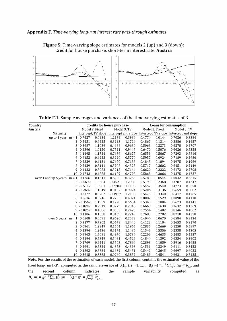
47
Appendix F. Time-varying long-run interest rate pass-through estimates
Figure 5. Time-varying slope estimates for models 2 (up) and 3 (down):
Credit for house purchase, short-term interest rate. Austria
-4
-3
-2
-1
0
1
2
3
4
1 8 15 22 29 36 43 50 57 64 71 78 85 92 99 106 113 120 127 134 141
-3
-2
-1
0
1
2
3
1 8 15 22 29 36 43 50 57 64 71 78 85 92 99 106 113 120 127 134 141
Table F.1. Sample averages and variances of the time-varying estimates of β
Country Credits for house purchase Loans for consumption
Austria
Maturity
Model 2. Fixed
intercept, TV slope
Model 3. TV
intercept and slope
Model 2. Fixed
intercept, TV slope
Model 3. TV
intercept and slope
up to 1 year m = 1 0.7427 0.0934 1.2139 0.3984 0.4774 0.0144 0.7026 0.3384
2 0.5451 0.6425 0.3293 1.1724 0.4867 0.1314 0.3886 0.1957
3 0.3687 1.1039 0.4688 0.9680 0.5063 0.2273 0.6278 0.4707
4 0.4396 1.0150 0.7521 0.9447 0.6470 0.5076 0.6626 0.5358
5 1.1495 1.1724 0.7636 0.8677 0.6559 0.5067 0.7293 0.5816
6 0.6152 0.4923 0.8290 0.5770 0.5957 0.0924 0.7189 0.2680
7 0.5329 0.4131 0.7670 0.7188 0.4845 0.1894 0.4975 0.1969
8 0.5129 0.5141 0.5908 0.4325 0.5717 0.2602 0.6451 0.2149
9 0.4123 0.5082 0.3215 0.7144 0.6620 0.2222 0.6172 0.2708
10 0.4742 0.4888 0.1109 0.4798 0.5868 0.3066 0.4275 0.4727
over 1 and up 5 years m = 1 0.1766 0.1541 0.6220 0.3265 0.5789 0.0544 1.0032 0.6615
2 -0.4690 1.3384 -0.4521 1.2982 0.5193 0.2368 0.3287 0.4347
3 -0.5112 1.3981 -0.2784 1.1106 0.5457 0.3540 0.4773 0.2550
4 -0.2687 1.1049 0.0187 0.9024 0.5206 0.3136 0.5659 0.3882
5 0.2327 0.8782 -0.1917 1.2108 0.5475 0.3340 0.6417 0.4765
6 0.0616 0.3746 0.2703 0.4821 0.8087 0.1529 1.0090 0.4118
7 -0.3562 1.1959 0.1228 0.5654 0.5343 0.1804 0.5673 0.4141
8 -0.0207 0.2919 0.0279 0.2346 0.6663 0.1630 0.7632 0.1369
9 -0.0257 0.4086 0.0333 0.2425 0.7554 0.1402 0.8146 0.4062
10 0.1106 0.1358 0.0159 0.2249 0.7683 0.2702 0.8710 0.4258
over 5 years m = 1 0.6508 0.0691 0.9620 0.2573 0.4044 0.0670 0.6584 0.3134
2 0.3177 0.7302 0.0679 1.3440 0.4122 0.1104 0.2653 0.3170
3 0.0961 1.2949 0.1664 1.1965 0.2835 0.2669 0.1250 0.5897
4 0.1394 1.2436 0.5174 1.1486 0.1546 0.5356 0.2338 0.4305
5 0.9963 1.4081 0.4970 1.0734 0.2206 0.4635 0.2483 0.4557
6 0.5194 0.5349 0.5481 0.4526 0.4844 0.1392 0.6354 0.2902
7 0.2769 0.4441 0.5503 0.7864 0.2898 0.1059 0.3916 0.1658
8 0.2691 0.5324 0.4373 0.4393 0.4531 0.2349 0.6111 0.3453
9 0.1863 0.5754 0.1639 0.5451 0.5442 0.3645 0.6697 0.6032
10 0.3615 0.3385 0.0760 0.3852 0.5489 0.4541 0.6621 0.7135
Note. For the results of the estimation of each model, the first column contains the estimated value of the
fixed long-run IRPT computed as the sample average of ˆ ( )t
mβ , t = 1, …, n, 1
1 0,ˆˆ( ) ( )n
n t t nm n m b−=β = β = , and
the second column indicates the sample variability computed as 1 2 2
1 1 ,ˆˆˆ ( ) ( ( ) ( ))n m
n t t n j j nm n m m b−= =σ = β − β = .

48
Figure 6. Time-varying slope estimates for models 2 (up) and 3 (down):
Credit for house purchase, short-term interest rate. Belgium
-3
-2
-1
0
1
2
3
4
1 5 9 13 17 21 25 29 33 37 41 45 49 53 57 61 65 69 73 77 81 85 89 93 97
-3
-2
-1
0
1
2
3
4
5
6
1 5 9 13 17 21 25 29 33 37 41 45 49 53 57 61 65 69 73 77 81 85 89 93 97
Table F.2. Sample averages and variances of the time-varying estimates of β
Country Credits for house purchase Loans for consumption
Belgium
Maturity
Model 2. Fixed
intercept, TV slope
Model 3. TV
intercept and slope
Model 2. Fixed
intercept, TV slope
Model 3. TV
intercept and slope
up to 1 year m = 1 0.7110 0.1904 -0.0740 0.8411 0.6493 0.2095 0.5372 0.1047
2 0.2675 0.3034 0.2593 0.3076 0.4414 0.1774 0.1688 0.5315
3 0.5031 0.7851 0.7810 1.0556 0.4323 1.2322 2.1233 3.1019
4 0.3666 1.1811 0.3504 0.6416 2.1804 3.3491 2.1684 3.8852
5 0.3344 0.6597 1.1689 1.3265 2.1626 3.8470 3.1183 4.2729
6 0.5744 0.2126 0.3998 0.4276 0.5502 0.2256 0.3092 0.1232
7 0.4939 0.8812 0.3017 0.7514 0.1440 0.5934 0.4985 0.2574
8 0.4771 0.4069 0.3432 0.4241 0.5294 0.2381 0.5268 0.9357
9 0.1467 0.4333 0.0587 0.6167 0.1077 0.7605 -0.1276 2.7949
10 -0.1455 0.8024 -0.1812 0.8268 -1.0432 4.0070 -0.3520 3.6559
over 1 and up 5 years m = 1 0.4330 0.1553 -0.1912 0.6656 0.5262 0.0369 -0.2617 0.9771
2 -0.4101 1.0439 -0.2385 0.8637 -0.6847 1.7054 -0.4372 1.4392
3 -0.1623 0.8695 0.7420 1.3017 -0.1507 1.6420 1.2133 2.4966
4 0.4601 0.7371 0.4593 0.7264 0.9188 1.5127 0.9144 1.6362
5 0.5152 0.8553 1.1129 0.9236 0.9572 1.8794 1.8750 2.0253
6 0.2143 0.1908 -0.0653 0.2783 0.2178 0.0870 -0.1315 0.4364
7 0.1542 0.4118 0.1579 0.2086 -0.2188 0.3772 -0.0943 0.3056
8 0.1888 0.1744 0.1921 0.2015 0.1592 0.2853 0.1729 0.4475
9 0.0665 0.2573 0.0150 0.3845 -0.4230 1.5253 -0.3028 1.7940
10 -0.0599 0.4621 -0.0126 0.4522 -0.9289 2.5817 -1.3046 2.8438
over 5 years m = 1 0.3262 0.0959 0.0445 0.2790 0.6469 0.0865 -1.0490 2.0969
2 -0.2587 0.8088 -0.1415 0.6777 -1.3250 2.5668 -1.0965 2.3265
3 -0.0603 0.7180 0.6476 1.1207 -0.9013 2.3533 0.6292 2.6933
4 0.4600 0.5900 0.4626 0.5943 0.0285 2.1009 0.0271 2.0779
5 0.5061 0.6984 1.0073 0.8369 0.1751 2.3105 1.6563 1.9357
6 0.1567 0.1234 0.0891 0.0607 0.1876 0.1610 -0.7368 1.2257
7 0.1367 0.3083 0.0906 0.2345 -0.2105 0.5293 -0.3697 0.3554
8 0.1367 0.1944 0.1114 0.1946 -0.2476 0.3868 -0.0012 0.3290
9 0.0258 0.1600 -0.0190 0.2810 -0.4783 1.2792 -0.6813 0.8556
10 -0.0893 0.3592 -0.0035 0.3490 -2.1829 2.8107 -1.0095 2.5822
Note. For the results of the estimation of each model, the first column contains the estimated value of the
fixed long-run IRPT computed as the sample average of ˆ ( )t
mβ , t = 1, …, n, 1
1 0,ˆˆ( ) ( )n
n t t nm n m b−=β = β = , and
the second column indicates the sample variability computed as 1 2 2
1 1 ,ˆˆˆ ( ) ( ( ) ( ))n m
n t t n j j nm n m m b−= =σ = β − β = .

49
Figure 7. Time-varying slope estimates for models 2 (up) and 3 (down):
Credit for house purchase, short-term interest rate. Finland
-0.5
0
0.5
1
1.5
2
2.5
1 8 15 22 29 36 43 50 57 64 71 78 85 92 99 106 113 120 127 134 141
-1
-0.5
0
0.5
1
1.5
2
2.5
1 8 15 22 29 36 43 50 57 64 71 78 85 92 99 106 113 120 127 134 141
Table F.3. Sample averages and variances of the time-varying estimates of β
Country Credits for house purchase Loans for consumption
Finland
Maturity
Model 2. Fixed
intercept, TV slope
Model 3. TV
intercept and slope
Model 2. Fixed
intercept, TV slope
Model 3. TV
intercept and slope
up to 1 year m = 1 0.8538 0.0918 0.9719 0.2040 0.5437 0.2443 0.8323 0.2486
2 0.6129 0.3697 0.6990 0.1704 0.5356 0.2103 0.4793 0.2963
3 0.7795 0.1070 0.8466 0.1930 0.7140 0.5115 1.0367 1.1734
4 0.7845 0.1563 0.9691 0.4179 0.8753 0.8773 0.8234 0.8021
5 0.9347 0.3681 0.6698 0.4116 0.8241 0.8040 0.8578 0.8282
6 0.8398 0.1563 0.9011 0.2868 0.7281 0.4106 0.8870 0.1243
7 0.7638 0.3347 0.8792 0.2996 0.5533 0.1945 0.4845 0.3604
8 0.8370 0.1892 0.8933 0.2758 0.5661 0.1936 0.7606 0.1474
9 0.6907 0.3117 0.5397 0.6736 0.8952 0.2878 0.8724 0.2743
10 0.6545 0.4211 0.2075 0.6558 0.8273 0.3171 0.5822 0.3648
over 1 and up 5 years m = 1 0.8373 0.0650 1.0514 0.2747 0.0821 0.2384 0.6479 0.6314
2 0.6643 0.3467 0.6953 0.2730 0.1249 0.2425 0.2434 0.2908
3 0.7315 0.2161 0.7740 0.1824 0.7058 1.5743 0.9570 2.1013
4 0.7085 0.3264 0.9218 0.5128 0.7152 1.6572 0.1963 1.1829
5 0.9992 0.6070 0.6730 0.4641 0.1142 1.7625 0.3886 2.2598
6 0.8032 0.2215 0.9457 0.3467 0.4946 0.6106 0.7144 0.1328
7 0.7710 0.3064 0.8952 0.3861 0.4534 0.1233 0.1312 0.6767
8 0.7685 0.2535 0.8587 0.3966 -0.0809 0.7842 -0.2072 0.5752
9 0.5851 0.4228 0.4347 0.6854 0.1123 0.9289 0.4798 1.3837
10 0.5588 0.4455 0.1377 0.6296 0.5086 1.8286 -0.1121 2.6484
over 5 years m = 1 0.8592 0.0357 1.1026 0.2776 -0.3916 0.0489 0.4533 1.1832
2 0.6416 0.4467 0.5965 0.5569 0.6638 1.4240 1.2967 2.5676
3 0.6039 0.5443 0.6367 0.5006 1.7964 3.9688 2.1463 4.6879
4 0.5560 0.6979 0.8710 0.8320 1.7503 3.9772 1.0237 3.1232
5 1.1155 1.0737 0.7355 0.6493 0.9708 3.2565 1.3201 3.8457
6 0.7997 0.3088 0.9315 0.3607 0.1734 0.5587 0.5430 0.6015
7 0.7062 0.3635 0.8497 0.4992 1.4581 1.2427 0.6348 0.7913
8 0.6502 0.2869 0.7902 0.4980 0.2519 1.3500 0.6168 1.1086
9 0.4553 0.4149 0.3116 0.6161 0.8018 1.1269 0.6139 1.3762
10 0.4507 0.4821 0.1030 0.5658 0.5184 1.5773 -0.1193 1.8280
Note. For the results of the estimation of each model, the first column contains the estimated value of the
fixed long-run IRPT computed as the sample average of ˆ ( )t
mβ , t = 1, …, n, 1
1 0,ˆˆ( ) ( )n
n t t nm n m b−=β = β = , and
the second column indicates the sample variability computed as 1 2 2
1 1 ,ˆˆˆ ( ) ( ( ) ( ))n m
n t t n j j nm n m m b−= =σ = β − β = .

50
Figure 8. Time-varying slope estimates for models 2 (up) and 3 (down):
Credit for house purchase, short-term interest rate. France
-4
-3
-2
-1
0
1
2
3
1 8 15 22 29 36 43 50 57 64 71 78 85 92 99 106 113 120 127 134 141
-3
-2.5
-2
-1.5
-1
-0.5
0
0.5
1
1.5
2
1 8 15 22 29 36 43 50 57 64 71 78 85 92 99 106 113 120 127 134 141
Table F.4. Sample averages and variances of the time-varying estimates of β
Country Credits for house purchase Loans for consumption
France
Maturity
Model 2. Fixed
intercept, TV slope
Model 3. TV
intercept and slope
Model 2. Fixed
intercept, TV slope
Model 3. TV
intercept and slope
up to 1 year m = 1 0.1128 0.1088 0.5361 0.3384 0.3742 0.1637 0.8993 0.9035
2 -0.0803 0.6176 -0.1460 0.7769 -0.1253 0.5161 -0.4150 1.0249
3 -0.3367 1.1094 -0.2573 0.9938 -0.2322 0.5430 -0.6081 1.2634
4 -0.2272 0.9497 0.1322 0.8135 -0.5323 1.1314 -0.3301 0.9029
5 0.5715 1.1034 0.4053 0.8276 -0.3370 0.9004 -0.0551 0.8272
6 0.0205 0.3155 0.3358 0.3776 0.6585 0.0929 0.8509 0.4289
7 -0.2024 0.6433 0.0636 0.3727 -0.1986 0.6687 -0.1530 1.0426
8 0.0933 0.2184 0.1909 0.1803 0.0824 0.2347 0.2875 0.3466
9 0.0590 0.2429 0.0566 0.2527 0.3918 0.3744 0.4326 0.8868
10 0.1751 0.2450 0.2151 0.3051 0.3548 0.7289 0.2916 0.6425
over 1 and up 5 years m = 1 0.0559 0.2412 0.6108 0.3728 0.2651 0.1661 0.5048 0.2251
2 0.0111 0.5762 -0.0912 0.8211 0.5218 0.2433 0.2686 0.3132
3 -0.1907 0.9933 -0.1108 0.8793 0.2829 0.2746 0.3422 0.1756
4 -0.0982 0.8609 0.1452 0.7475 0.2732 0.2787 0.2309 0.3492
5 0.4940 0.8890 0.3668 0.7179 0.2113 0.4986 0.3412 0.6271
6 -0.0455 0.2250 0.3646 0.4348 0.2683 0.1689 0.5015 0.4798
7 -0.0871 0.5074 0.1366 0.3813 0.2188 0.1837 0.1230 0.2103
8 0.0661 0.2233 0.0881 0.2042 0.1457 0.9309 0.2432 0.8074
9 0.0265 0.2759 0.0087 0.3246 0.3337 0.5807 0.3660 0.5465
10 -0.0250 0.4236 -0.0701 0.4046 0.3135 0.6031 0.3052 0.6536
over 5 years m = 1 0.0203 0.3127 0.4719 0.2437 0.2308 0.0980 0.4466 0.2356
2 0.0974 0.4008 -0.0173 0.6656 0.4698 0.2617 0.2144 0.2961
3 -0.0402 0.7047 -0.0120 0.6641 0.1781 0.3992 0.3603 0.1364
4 -0.0087 0.6588 0.1298 0.5874 0.2916 0.1716 0.1966 0.3242
5 0.4409 0.6904 0.3845 0.6019 0.1837 0.4323 0.4059 0.7329
6 -0.0570 0.0422 0.2738 0.2663 0.2179 0.0864 0.4353 0.4997
7 -0.0078 0.3037 0.0963 0.2369 0.1787 0.2877 -0.0019 0.3102
8 0.0165 0.1318 -0.0028 0.1516 0.0414 1.0648 0.3599 1.0209
9 -0.0528 0.2241 -0.1212 0.2745 0.5212 0.6841 0.6092 0.6669
10 -0.0786 0.2627 -0.0412 0.2560 0.5980 0.7053 0.7183 0.8222
Note. For the results of the estimation of each model, the first column contains the estimated value of the
fixed long-run IRPT computed as the sample average of ˆ ( )t
mβ , t = 1, …, n, 1
1 0,ˆˆ( ) ( )n
n t t nm n m b−=β = β = , and
the second column indicates the sample variability computed as 1 2 2
1 1 ,ˆˆˆ ( ) ( ( ) ( ))n m
n t t n j j nm n m m b−= =σ = β − β = .

51
Figure 9. Time-varying slope estimates for models 2 (up) and 3 (down):
Credit for house purchase, short-term interest rate. Germany
-5
-4
-3
-2
-1
0
1
2
3
4
1 8 15 22 29 36 43 50 57 64 71 78 85 92 99 106 113 120 127 134 141
-4
-3
-2
-1
0
1
2
3
1 8 15 22 29 36 43 50 57 64 71 78 85 92 99 106 113 120 127 134 141
Table F.5. Sample averages and variances of the time-varying estimates of β
Country Credits for house purchase Loans for consumption
Germany
Maturity
Model 2. Fixed
intercept, TV slope
Model 3. TV
intercept and slope
Model 2. Fixed
intercept, TV slope
Model 3. TV
intercept and slope
up to 1 year m = 1 0.6015 0.0795 0.8939 0.2304 0.3609 0.0216 0.0980 0.3992
2 0.4234 0.4959 0.1774 1.1021 -0.4686 1.0659 -0.6679 1.4305
3 0.1598 1.1329 0.2313 1.0309 -0.3098 0.7120 0.1728 1.0810
4 0.2004 1.0885 0.5421 1.0273 0.3524 1.3766 0.4580 1.5599
5 0.9438 1.2609 0.7202 0.9592 0.4562 1.5472 0.3287 1.5950
6 0.4915 0.4262 0.5768 0.3470 0.3605 0.0213 0.1458 0.5611
7 0.3270 0.2969 0.4913 0.4831 -0.4908 0.9519 -0.2124 0.8765
8 0.4018 0.2652 0.5040 0.3771 0.0590 0.6579 0.2172 0.6872
9 0.4071 0.2635 0.3103 0.4632 0.2924 0.5986 0.4031 0.6957
10 0.4512 0.5805 0.1923 0.3894 0.4842 0.5753 0.4727 0.5576
over 1 and up 5 years m = 1 0.1948 0.1984 0.6703 0.3250 0.1421 0.1826 0.1389 0.1866
2 0.1775 0.4568 -0.0993 1.1329 0.7079 0.5527 0.5281 0.2439
3 -0.2160 1.3383 -0.1183 1.1953 0.4819 0.1853 0.5491 0.2489
4 -0.1033 1.1707 0.1434 1.0461 0.4210 0.2305 0.3750 0.2959
5 0.7282 1.2662 0.6174 1.0894 0.3830 0.2398 0.3280 0.2483
6 0.0736 0.3583 0.3838 0.3816 0.0197 0.0721 0.1591 0.3349
7 0.0203 0.3372 0.1418 0.2510 0.4790 0.5307 0.3270 0.1883
8 0.1252 0.1455 0.1328 0.1354 0.3175 0.3582 0.2503 0.4303
9 0.0921 0.1770 -0.0017 0.2509 0.2166 0.3878 0.1972 0.5014
10 0.0852 0.2248 -0.0038 0.1881 0.1457 0.6199 0.2444 0.7853
over 5 years m = 1 0.0717 0.3206 0.4606 0.1985 0.2484 0.0037 0.1093 0.2046
2 0.2367 0.2606 -0.0680 0.9710 0.4389 0.2174 0.3678 0.1007
3 -0.0738 0.9811 -0.0765 0.9852 0.2317 0.3604 0.1497 0.5305
4 -0.0549 0.9453 0.1228 0.8500 0.1794 0.4748 0.2373 0.3888
5 0.5704 0.9772 0.5450 0.9354 0.2502 0.3897 0.3212 0.3207
6 -0.0308 0.1506 0.1828 0.2124 0.1127 0.1187 0.0897 0.0248
7 0.0079 0.0350 0.0317 0.1537 0.3278 0.2034 0.2755 0.1044
8 0.0358 0.1129 0.0539 0.0862 0.2633 0.0824 0.4189 0.2234
9 0.0506 0.0939 0.0147 0.1139 0.5245 0.2535 0.5467 0.2155
10 0.0495 0.0920 0.0079 0.0910 0.5657 0.3778 0.5035 0.2853
Note. For the results of the estimation of each model, the first column contains the estimated value of the
fixed long-run IRPT computed as the sample average of ˆ ( )t
mβ , t = 1, …, n, 1
1 0,ˆˆ( ) ( )n
n t t nm n m b−=β = β = , and
the second column indicates the sample variability computed as 1 2 2
1 1 ,ˆˆˆ ( ) ( ( ) ( ))n m
n t t n j j nm n m m b−= =σ = β − β = .

52
Figure 10. Time-varying slope estimates for models 2 (up) and 3 (down):
Credit for house purchase, short-term interest rate. Italy
-2
-1
0
1
2
3
4
5
1 8 15 22 29 36 43 50 57 64 71 78 85 92 99 106 113 120 127 134 141
-3
-2
-1
0
1
2
3
4
5
6
1 8 15 22 29 36 43 50 57 64 71 78 85 92 99 106 113 120 127 134 141
Table F.6. Sample averages and variances of the time-varying estimates of β
Country Credits for house purchase Loans for consumption
Italy
Maturity
Model 2. Fixed
intercept, TV slope
Model 3. TV
intercept and slope
Model 2. Fixed
intercept, TV slope
Model 3. TV
intercept and slope
up to 1 year m = 1 0.5170 0.2306 0.7395 0.4399 0.8559 0.5814 0.1812 1.2204
2 0.3595 0.2812 0.9124 1.1888 -0.8255 2.6540 -1.5751 4.4121
3 1.0003 1.3441 1.0117 1.3620 -0.7700 3.0694 -0.5567 2.8105
4 0.8925 1.1851 0.9219 1.2165 -0.5485 2.8033 0.2864 2.2557
5 0.5613 0.9229 0.1556 1.3266 0.8007 2.2440 -0.0241 2.5254
6 0.5806 0.0615 0.9142 0.4368 0.5968 0.6091 -1.0041 0.8514
7 0.7930 0.4351 1.0910 1.0336 -0.9640 1.3133 -0.2936 1.3668
8 0.6539 0.7317 0.7534 0.6845 0.1967 1.3462 0.7491 1.4209
9 0.4626 0.7427 0.5598 0.7529 1.0183 1.7266 1.2505 1.9212
10 0.9224 0.9809 0.8883 0.9081 0.7296 1.8278 -0.2724 1.6555
over 1 and up 5 years m = 1 0.5635 0.0845 0.7425 0.2576 -0.0159 0.2650 0.3098 0.1666
2 0.2451 0.5247 0.2536 0.5043 -0.0967 0.5184 0.0277 0.2724
3 0.1142 0.7447 0.2598 0.5565 0.0863 0.2276 0.0107 0.2820
4 0.2254 0.6031 0.3820 0.5638 -0.1318 0.7547 0.2964 1.1394
5 0.5703 0.6410 0.3218 0.5847 0.3651 1.2178 0.2447 0.9835
6 0.5202 0.2834 0.6701 0.2517 -0.0492 0.1121 0.2419 0.1564
7 0.3941 0.5636 0.5536 0.2527 -0.1146 0.5890 0.0711 0.7224
8 0.3990 0.2246 0.4391 0.3464 0.2537 0.4506 0.5944 0.8704
9 0.2921 0.2099 0.1386 0.2476 0.5510 0.6816 0.7225 1.1017
10 0.2937 0.2469 0.1202 0.2960 0.3966 0.7995 0.0356 1.2861
over 5 years m = 1 0.6258 0.0162 0.8558 0.2467 0.0865 0.2686 0.1624 0.3371
2 0.3646 0.5152 0.3364 0.5841 0.2889 0.5044 0.9182 2.0114
3 0.2502 0.7332 0.3685 0.5774 1.0239 2.1976 0.7057 1.7475
4 0.3379 0.6217 0.5574 0.5895 0.5308 1.6820 0.6032 1.7721
5 0.7831 0.7355 0.4947 0.5720 0.2976 1.4300 0.6032 1.9395
6 0.5648 0.2962 0.7094 0.2874 0.2183 0.3370 0.5663 0.2048
7 0.4432 0.4750 0.6500 0.4182 0.3473 0.1257 0.3476 0.6790
8 0.4876 0.2205 0.5436 0.2835 0.3395 0.3172 0.5172 0.4956
9 0.4072 0.2369 0.2667 0.3989 0.4158 0.5570 0.4169 0.5338
10 0.3935 0.3006 0.0801 0.4532 0.1785 0.5235 0.0194 0.5506
Note. For the results of the estimation of each model, the first column contains the estimated value of the
fixed long-run IRPT computed as the sample average of ˆ ( )t
mβ , t = 1, …, n, 1
1 0,ˆˆ( ) ( )n
n t t nm n m b−=β = β = , and
the second column indicates the sample variability computed as 1 2 2
1 1 ,ˆˆˆ ( ) ( ( ) ( ))n m
n t t n j j nm n m m b−= =σ = β − β = .
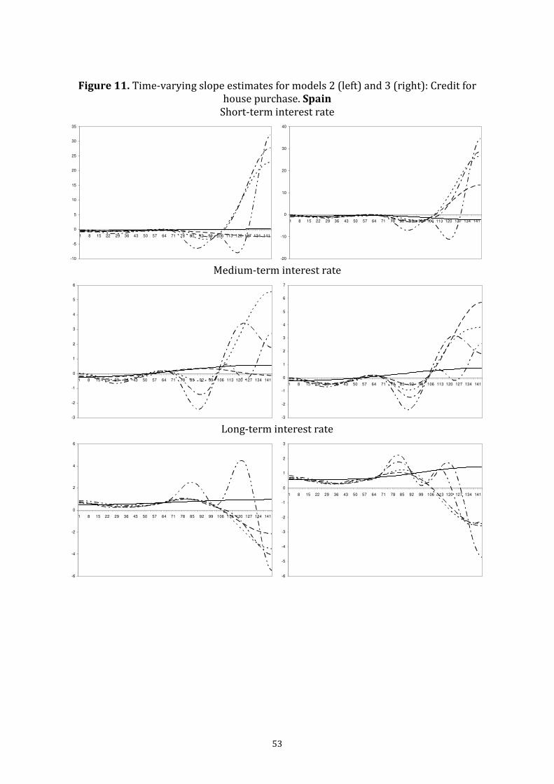
53
Figure 11. Time-varying slope estimates for models 2 (left) and 3 (right): Credit for
house purchase. Spain
Short-term interest rate
-10
-5
0
5
10
15
20
25
30
35
1 8 15 22 29 36 43 50 57 64 71 78 85 92 99 106 113 120 127 134 141
-20
-10
0
10
20
30
40
1 8 15 22 29 36 43 50 57 64 71 78 85 92 99 106 113 120 127 134 141
Medium-term interest rate
-3
-2
-1
0
1
2
3
4
5
6
1 8 15 22 29 36 43 50 57 64 71 78 85 92 99 106 113 120 127 134 141
-3
-2
-1
0
1
2
3
4
5
6
7
1 8 15 22 29 36 43 50 57 64 71 78 85 92 99 106 113 120 127 134 141
Long-term interest rate
-6
-4
-2
0
2
4
6
1 8 15 22 29 36 43 50 57 64 71 78 85 92 99 106 113 120 127 134 141
-6
-5
-4
-3
-2
-1
0
1
2
3
1 8 15 22 29 36 43 50 57 64 71 78 85 92 99 106 113 120 127 134 141

54
Table F.7. Sample averages and variances of the time-varying estimates of β
Country Credits for house purchase Loans for consumption
Spain
Maturity
Model 2. Fixed
intercept, TV slope
Model 3. TV
intercept and slope
Model 2. Fixed
intercept, TV slope
Model 3. TV
intercept and slope
up to 1 year m = 1 -0.1665 0.1858 -0.9629 0.6513 0.8666 0.1944 0.8358 0.1585
2 -1.0048 0.7110 1.0536 4.5748 -0.4519 1.4481 -1.1799 2.8262
3 2.5481 7.2290 3.0556 8.0456 -1.2648 3.0664 -1.2362 3.0089
4 3.1275 8.2302 2.4914 8.0208 -0.8612 2.3897 -0.8435 2.3686
5 0.0726 8.1450 -0.3822 8.7138 -0.8995 2.4940 -0.3772 2.3905
6 0.2112 1.5503 -0.3432 0.7669 0.7738 0.2782 0.7135 0.2889
7 0.6296 0.8857 1.8250 3.2194 -1.0427 1.4681 -0.8365 1.9969
8 2.7121 3.9149 2.5203 4.1632 -0.4317 1.7908 0.0188 1.5883
9 2.6660 4.0504 1.2418 4.8943 0.2656 1.0040 1.0180 2.0216
10 2.5162 4.0665 1.7296 3.8697 0.6059 2.2501 0.5834 2.0728
over 1 and up 5 years m = 1 0.1726 0.2971 0.2197 0.3390 -0.1053 0.0286 0.5050 0.9086
2 0.0310 0.2059 0.7799 1.8446 -0.2825 0.3319 0.0543 0.6037
3 0.7586 1.8069 0.5186 1.4623 0.6663 2.3548 0.8444 2.7287
4 0.3893 1.3821 0.3455 1.3326 1.0088 3.0406 0.6341 2.4504
5 -0.2793 0.9874 -0.2539 0.9750 0.5753 2.4121 0.6639 2.5326
6 0.3196 0.3784 0.6183 0.2595 0.4520 0.4744 0.5639 0.0552
7 0.2294 0.4993 0.2970 0.2171 0.4213 0.1410 0.5564 0.1141
8 0.0029 0.4845 0.0673 0.5340 0.4424 0.7882 0.5744 0.5964
9 -0.2279 0.4909 -0.1112 0.5558 0.6703 0.4319 0.8998 0.8439
10 0.0611 0.5669 0.0729 0.3895 0.8022 0.6998 0.6835 0.6744
over 5 years m = 1 0.7209 0.1697 0.8850 0.3241 -0.1030 0.1206 0.6718 1.2262
2 0.0918 0.9207 0.0333 1.0635 -0.1662 0.4570 -0.1202 0.4796
3 -0.1111 1.3132 0.0361 1.1137 0.2121 1.2034 0.0392 0.8749
4 -0.0648 1.3132 0.4076 1.3457 0.2047 1.1653 0.2440 1.2326
5 0.9416 1.7688 0.3646 1.1495 0.2426 1.2266 0.3762 1.3419
6 0.6230 0.6193 0.6322 0.3910 0.3784 0.3138 0.6593 0.4948
7 0.2250 0.8173 0.5883 0.9575 0.1825 0.1284 0.2742 0.2077
8 0.1625 0.4445 0.3545 0.4949 0.3944 0.6345 0.5389 0.5837
9 0.0122 0.5192 0.0341 0.4064 0.6545 0.5303 0.5922 0.6004
10 0.2341 0.2087 0.0590 0.3538 0.5774 0.6266 0.5153 0.6365
Note. For the results of the estimation of each model, the first column contains the estimated value of the
fixed long-run IRPT computed as the sample average of ˆ ( )t
mβ , t = 1, …, n, 1
1 0,ˆˆ( ) ( )n
n t t nm n m b−=β = β = , and
the second column indicates the sample variability computed as 1 2 2
1 1 ,ˆˆˆ ( ) ( ( ) ( ))n m
n t t n j j nm n m m b−= =σ = β − β = .