WHOI-2008-04

Woods Hole Oceanographic Institution

WHOI Hawaii Ocean Timeseries Station (WHOTS): WHOTS-4 2007 Mooring Turnaround Cruise Report

by

Sean P. Whelan, Al Plueddemann, Roger Lukas, Jeffrey Lord, Paul Lethaby, Jeffrey Snyder, Jason Smith, Frank Bahr, Nan Galbraith and Chris Sabine

Woods Hole Oceanographic Institution, Woods Hole, Massachusetts

January 2008

Technical Report

Funding was provided by the National Oceanic and Atmospheric Administration under Grant No. NA17RJ1223 for the Cooperative Institute for Climate and Ocean Research (CICOR).

Approved for public release; distribution unlimited.

UP

PE

RO

CE

AN

P R O C E S S E SG

RO

UP

•W

HO

I

Upper Ocean Processes GroupWoods Hole Oceanographic InstitutionWoods Hole, MA 02543UOP Technical Report 2008-02

iii

Abstract

The Woods Hole Oceanographic Institution (WHOI) Hawaii Ocean Timeseries (HOT) Site (WHOTS), 100 km north of Oahu, Hawaii, is intended to provide long-term, high-quality air-sea fluxes as a part of the NOAA Climate Observation Program. The WHOTS mooring also serves as a coordinated part of the HOT program, contributing to the goals of observing heat, fresh water and chemical fluxes at a site representative of the oligotrophic North Pacific Ocean. The approach is to maintain a surface mooring outfitted for meteorological and oceanographic measurements at a site near 22.75°N, 158°W by successive mooring turnarounds. These observations will be used to investigate air–sea interaction processes related to climate variability.

The first three WHOTS moorings (WHOTS-1 through 3) were deployed in August 2004, July 2005 and June 2006, respectively. This report documents recovery of the WHOTS-3 mooring and deployment of the fourth mooring (WHOTS-4). Both moorings used Surlyn foam buoys as the surface element and were outfitted with two Air–Sea Interaction Meteorology (ASIMET) systems. Each ASIMET system measures, records, and transmits via Argos satellite the surface meteorological variables necessary to compute air–sea fluxes of heat, moisture and momentum. The upper 155 m of the moorings were outfitted with oceanographic sensors for the measurement of temperature, conductivity and velocity in a cooperative effort with R. Lukas of the University of Hawaii. A pCO2 system was installed on the WHOT-3 buoy in a cooperative effort with Chris Sabine at the Pacific Marine Environmental Laboratory.

The WHOTS mooring turnaround was done on the University of Hawaii research vessel

Kilo Moana, Cruise KM-07-08, by the Upper Ocean Processes Group of the Woods Hole Oceanographic Institution. The cruise took place between 24 June and 1 July 2007. Operations began with deployment of the WHOTS-4 mooring on 25 June at approximately 22°40.2′N, 157°57.0′W in 4756 m of water. This was followed by meteorological intercomparisons and CTDs at the WHOTS-4 and WHOTS-3 sites. The WHOTS-3 mooring was recovered on June 28th followed by CTD operations at the HOT site and shipboard meteorological observations at several sites to the south of the mooring site. This report describes these cruise operations, as well as some of the in-port operations and pre-cruise buoy preparations.

iv

Table of Contents Page No.

Abstract ................................................................................................................................................. iii List of Figures .........................................................................................................................................v List of Tables .........................................................................................................................................vi 1. Introduction .....................................................................................................................................1

2. Pre-Cruise Operations ....................................................................................................................3 a. Staging and Loading....................................................................................................................3 b. Buoy Spins ..................................................................................................................................3 c. Sensor Evaluation ........................................................................................................................5 d. AutoIMET system on the Kilo Moana ........................................................................................7

3. WHOTS-4 Mooring Description ..................................................................................................10 a. Mooring Design.........................................................................................................................10 b. Bird Barrier................................................................................................................................12 c. Anti-fouling Treatment..............................................................................................................12 d. Buoy Instrumentation ...............................................................................................................13 e. Subsurface Instrumentation .......................................................................................................18

4. WHOTS-4 Mooring Deployment..................................................................................................20 a. Bathymetry ................................................................................................................................20 b. Deployment Approach...............................................................................................................21 c. Deployment Operations .............................................................................................................22 d. Anchor Survey...........................................................................................................................27

5. WHOTS-3 Mooring Recovery ......................................................................................................29 a. Recovery Operations .................................................................................................................29 b. Surface Instrumentation and Data Return .................................................................................30 c. Subsurface Instrumentation and Data Return ............................................................................39 d. Bird Wire Effectiveness ............................................................................................................45 e. Biofouling..................................................................................................................................46 f. Wind Vane Evaluation ...............................................................................................................47

6. Meteorological Intercomparison .................................................................................................50 a. Overview ...................................................................................................................................50 b. WHOTS-3 vs. Kilo Moana........................................................................................................50 c. WHOTS-4 vs. Kilo Moana ........................................................................................................54

7. CTD Operations ...........................................................................................................................58

Acknowledgments.................................................................................................................................58 References.............................................................................................................................................59 Appendix A. WHOI 2007 Science Party .............................................................................................60 Appendix B. Sand Island Port Contacts...............................................................................................61 Appendix C. CTD Casts ......................................................................................................................63 Appendix D. WHOTS-3 Recovered Subsurface Plots.........................................................................86 Appendix E. WHOTS-3 Moored Station Deployed and Recovered..................................................101 Appendix F. WHOTS-4 Moored Station Deployed...........................................................................107

v

List of Figures Page No.

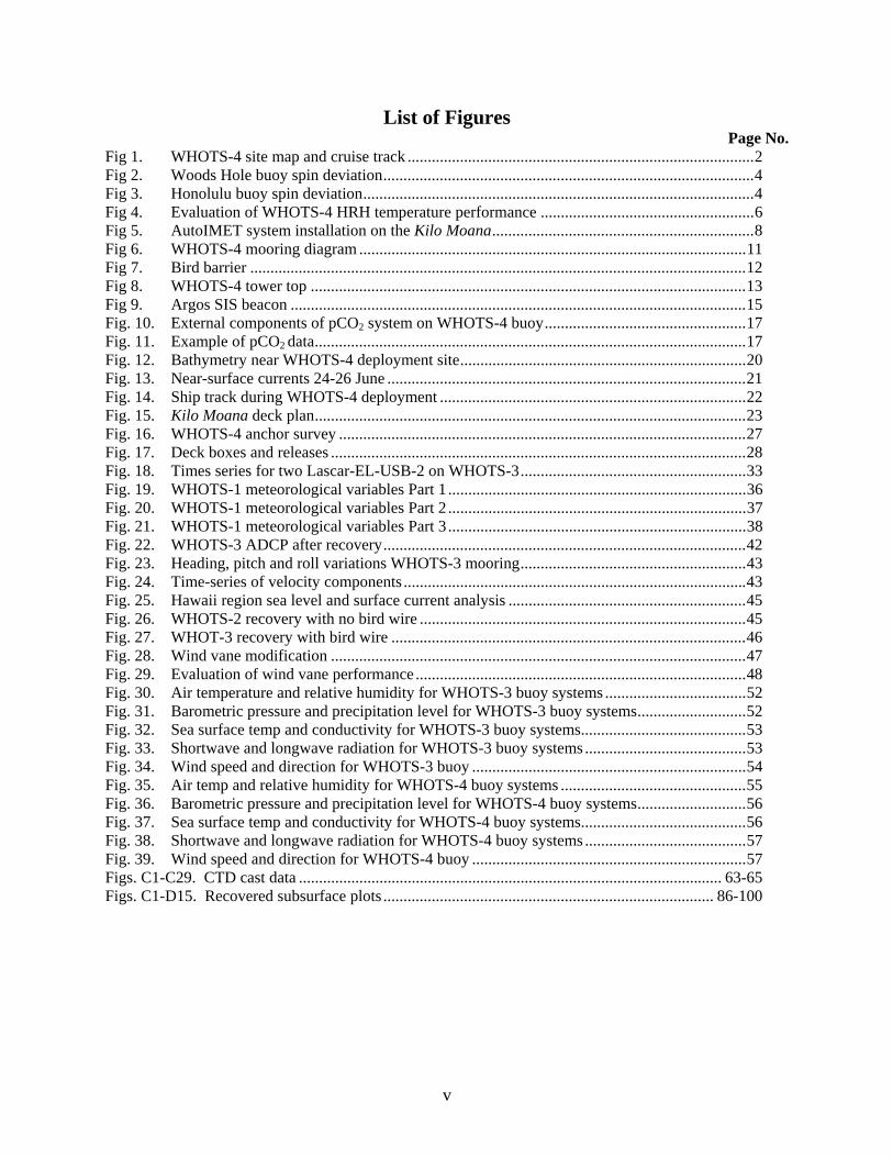
Fig 1. WHOTS-4 site map and cruise track ......................................................................................2 Fig 2. Woods Hole buoy spin deviation............................................................................................4 Fig 3. Honolulu buoy spin deviation.................................................................................................4 Fig 4. Evaluation of WHOTS-4 HRH temperature performance .....................................................6 Fig 5. AutoIMET system installation on the Kilo Moana.................................................................8 Fig 6. WHOTS-4 mooring diagram ................................................................................................11 Fig 7. Bird barrier ...........................................................................................................................12 Fig 8. WHOTS-4 tower top ............................................................................................................13 Fig 9. Argos SIS beacon .................................................................................................................15 Fig. 10. External components of pCO2 system on WHOTS-4 buoy..................................................17 Fig. 11. Example of pCO2 data...........................................................................................................17 Fig. 12. Bathymetry near WHOTS-4 deployment site.......................................................................20 Fig. 13. Near-surface currents 24-26 June .........................................................................................21 Fig. 14. Ship track during WHOTS-4 deployment ............................................................................22 Fig. 15. Kilo Moana deck plan...........................................................................................................23 Fig. 16. WHOTS-4 anchor survey .....................................................................................................27 Fig. 17. Deck boxes and releases .......................................................................................................28 Fig. 18. Times series for two Lascar-EL-USB-2 on WHOTS-3........................................................33 Fig. 19. WHOTS-1 meteorological variables Part 1 ..........................................................................36 Fig. 20. WHOTS-1 meteorological variables Part 2 ..........................................................................37 Fig. 21. WHOTS-1 meteorological variables Part 3 ..........................................................................38 Fig. 22. WHOTS-3 ADCP after recovery..........................................................................................42 Fig. 23. Heading, pitch and roll variations WHOTS-3 mooring........................................................43 Fig. 24. Time-series of velocity components .....................................................................................43 Fig. 25. Hawaii region sea level and surface current analysis ...........................................................45 Fig. 26. WHOTS-2 recovery with no bird wire .................................................................................45 Fig. 27. WHOT-3 recovery with bird wire ........................................................................................46 Fig. 28. Wind vane modification .......................................................................................................47 Fig. 29. Evaluation of wind vane performance ..................................................................................48 Fig. 30. Air temperature and relative humidity for WHOTS-3 buoy systems ...................................52 Fig. 31. Barometric pressure and precipitation level for WHOTS-3 buoy systems...........................52 Fig. 32. Sea surface temp and conductivity for WHOTS-3 buoy systems.........................................53 Fig. 33. Shortwave and longwave radiation for WHOTS-3 buoy systems ........................................53 Fig. 34. Wind speed and direction for WHOTS-3 buoy ....................................................................54 Fig. 35. Air temp and relative humidity for WHOTS-4 buoy systems ..............................................55 Fig. 36. Barometric pressure and precipitation level for WHOTS-4 buoy systems...........................56 Fig. 37. Sea surface temp and conductivity for WHOTS-4 buoy systems.........................................56 Fig. 38. Shortwave and longwave radiation for WHOTS-4 buoy systems ........................................57 Fig. 39. Wind speed and direction for WHOTS-4 buoy ....................................................................57 Figs. C1-C29. CTD cast data ......................................................................................................... 63-65 Figs. C1-D15. Recovered subsurface plots .................................................................................. 86-100

vi

List of Tables

Page No. Table 1. WHOTS-4 ASIMET system composition ............................................................................14 Table 2. Argos beacon specifications .................................................................................................15 Table 3. WHOTS-4 VMCM configuration.........................................................................................18 Table 4. WHOTS-4 mooring ADCP deployment information...........................................................18 Table 5. WHOTS-4 Mooring - Microcat deployment information ....................................................19 Table 6. Survey sites and milliseconds...............................................................................................28 Table 7. WHOTS-3 ASIMET system configuration ..........................................................................30 Table 8. WHOTS-3 ASIMET sensor specification ............................................................................31 Table 9. WHOTS-2 ASIMET module heights and separations..........................................................31 Table 10. Lascar EL-USB-2 performance ............................................................................................34 Table 11. Lascar EL-USB-2 sample and memory................................................................................34 Table 12. WHOTS-3 Microcat/Seacat deployment information ..........................................................39 Table 13. WHOTS-3 Microcat/Seacat recovery information ...............................................................40 Table 14. WHOTS-3 VMCMs .............................................................................................................41 Table 15. WHOTS-3 ADCP deployment and recovery information....................................................41

1

1. Introduction

The Hawaii Ocean Timeseries (HOT) site, 100 km north of Oahu, Hawaii, has been occupied since 1988 as a part of the World Ocean Circulation Experiment (WOCE) and the Joint Global Ocean Flux Study (JGOFS). The present HOT program includes comprehensive, interdisciplinary upper ocean observations, but does not include continuous surface forcing measurements. Thus, a primary driver for the WHOTS mooring is to provide long-term, high-quality air-sea fluxes as a coordinated part of the HOT program and to contribute to the program goals of observing heat, fresh water and chemical fluxes at a site representative of the oligotrophic North Pacific Ocean. The WHOTS mooring also serves as an Ocean Reference Station – a part of NOAA’s Ocean Observing System for Climate – providing time-series of accurate surface meteorology, air-sea fluxes, and upper ocean variability to quantify air-sea exchanges of heat, freshwater, and momentum, to describe the local oceanic response to atmospheric forcing, to motivate and guide improvement to atmospheric, oceanic, and coupled models, to calibrate and guide improvement to remote sensing products, and to provide anchor point for the development of new, basin scale air-sea flux fields.

To accomplish these objectives, a surface mooring with sensors suitable for the determination of air–sea fluxes and upper ocean properties is being maintained at a site near 22°45′N, 158°00′W (Figure 1) by means of annual “turnarounds” (recovery of one mooring and deployment of a new mooring near the same site). The moorings use Surlyn foam buoys as the surface element, outfitted with two complete Air–Sea Interaction Meteorology (ASIMET) systems. Each system measures, records, and transmits via Argos satellite the surface meteorological variables necessary to compute air–sea fluxes of heat, moisture and momentum.

Subsurface observations have been made on all WHOTS deployments in cooperation

with Roger Lukas at the University of Hawaii (UH). The upper 155 m of the mooring line is outfitted with oceanographic sensors for the measurement of temperature, conductivity and velocity. For WHOTS-3, a pCO2 system for investigation of the air-sea exchange of CO2 at the ocean surface was mounted in the buoy well in cooperation with Chris Sabine at the Pacific Marine Environmental Laboratory (PMEL).

The mooring turnaround was done on the UH Research Vessel Kilo Moana, cruise KM-

07-08, by the Upper Ocean Processes Group (UOP) of the Woods Hole Oceanographic Institution (WHOI) with assistance from the UH personnel. The cruise was completed in 8 days, between 24 June and 1 July 2007. The cruise originated from, and returned to, Honolulu, HI (Figure 1). The facilities of the UH Marine Center at Sand Island, and a tent maintained by the Hawaii Undersea Research Lab, were used for pre-cruise staging.

2

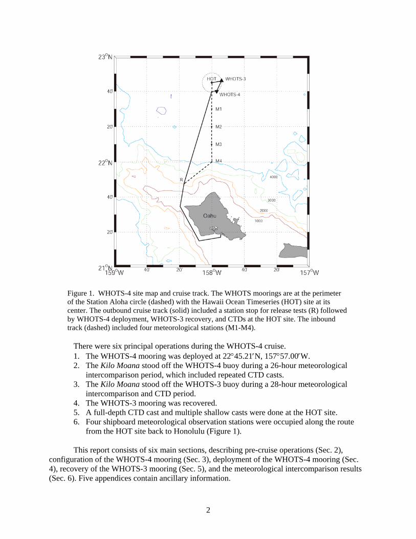
Figure 1. WHOTS-4 site map and cruise track. The WHOTS moorings are at the perimeter of the Station Aloha circle (dashed) with the Hawaii Ocean Timeseries (HOT) site at its center. The outbound cruise track (solid) included a station stop for release tests (R) followed by WHOTS-4 deployment, WHOTS-3 recovery, and CTDs at the HOT site. The inbound track (dashed) included four meteorological stations (M1-M4).

There were six principal operations during the WHOTS-4 cruise. 1. The WHOTS-4 mooring was deployed at 22°45.21′N, 157°57.00′W. 2. The Kilo Moana stood off the WHOTS-4 buoy during a 26-hour meteorological

intercomparison period, which included repeated CTD casts. 3. The Kilo Moana stood off the WHOTS-3 buoy during a 28-hour meteorological

intercomparison and CTD period. 4. The WHOTS-3 mooring was recovered. 5. A full-depth CTD cast and multiple shallow casts were done at the HOT site. 6. Four shipboard meteorological observation stations were occupied along the route

from the HOT site back to Honolulu (Figure 1). This report consists of six main sections, describing pre-cruise operations (Sec. 2),

configuration of the WHOTS-4 mooring (Sec. 3), deployment of the WHOTS-4 mooring (Sec. 4), recovery of the WHOTS-3 mooring (Sec. 5), and the meteorological intercomparison results (Sec. 6). Five appendices contain ancillary information.

3

2. Pre-Cruise Operations

a. Staging and Loading Pre-cruise operations were conducted on the grounds of the UH Marine Center in

Honolulu, HI. A shipment consisting of (1) 40’ container left Woods Hole for Honolulu on 09 June 2006. The container held the buoy well, tower mid-section, tower top with modules, spare modules, VMCMs, acoustic releases and deck gear, instrument brackets and load bars, primary mooring components, deck boxes, lab boxes, anchor modules.

A second 40' container left WHOI on 16 June, 2006 and was delivered directly to the

Revelle at Pier 31. This container held most of the spare mooring components, winding cart, tension cart, and dragging gear. We used the ship's TSE winch. Many of the spares and support gear were already in Hawaii and we moved them to the ship with the rest of the gear, including the foam hull.

Three UOP representatives arrived in Honolulu on June 14, and began offloading the gear

to a staging area near the dock. UH personnel also assisted with in-port preparations. The UOP group was grateful for access to the Hawaii Undersea Research Laboratory (HURL) tent to house gear not suitable for outside storage and for use as a staging for electronics. Pre-cruise operations took place from June 14, prior to departure of the Kilo Moana on 24 June. In addition to loading the ship, pre-cruise operations included: assembly of primary and spare anchor, assembly of glass balls onto 4 m chain sections, painting of the buoy hull, assembly of the buoy tower top, insertion of the tower top assembly into the foam buoy hull, a buoy spin, evaluation of ASIMET data, and preparation of the oceanographic instruments.

Because continued pre-cruise work in Hawaii is anticipated, space is rented in containers

on the UH Marine Center site; therefore, not all recovered gear was shipped back to WHOI. Items left at the Marine Center included the assembled buoy hull, a spare anchor, approximately 80 glass balls, and spare wire, nylon, and polypropylene. b. Buoy Spins

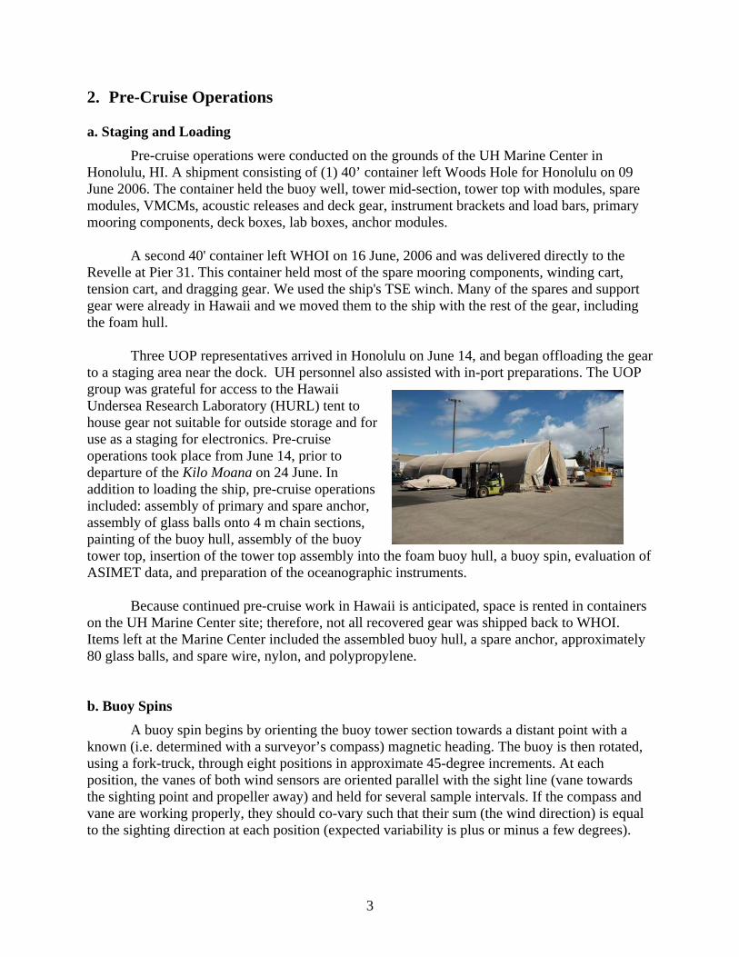
A buoy spin begins by orienting the buoy tower section towards a distant point with a known (i.e. determined with a surveyor’s compass) magnetic heading. The buoy is then rotated, using a fork-truck, through eight positions in approximate 45-degree increments. At each position, the vanes of both wind sensors are oriented parallel with the sight line (vane towards the sighting point and propeller away) and held for several sample intervals. If the compass and vane are working properly, they should co-vary such that their sum (the wind direction) is equal to the sighting direction at each position (expected variability is plus or minus a few degrees).

4

The first buoy spins were done in the parking lot outside the WHOI Clark Laboratory high bay, with care taken to ensure that cars were not parked within about 30 ft of the buoy. The sighting angle to “the big tree” was about 310°, WHOI buoy spin. Figure 2 shows the Woods Hole deviation results graphically.

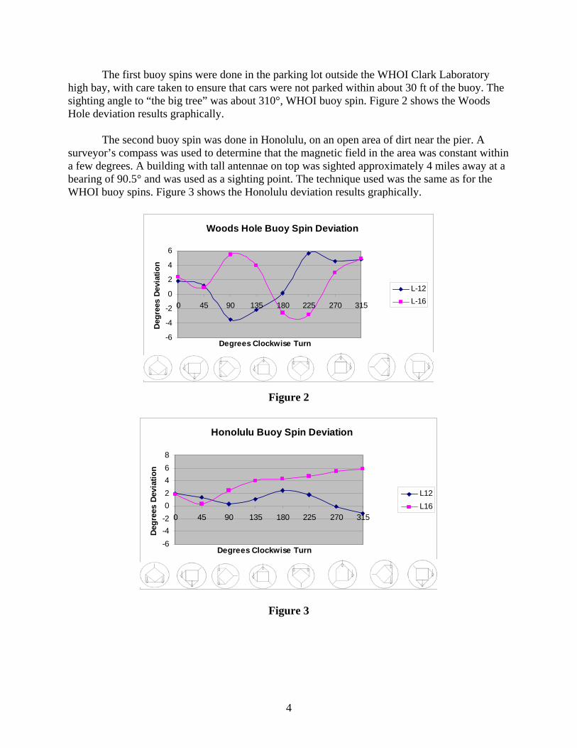
The second buoy spin was done in Honolulu, on an open area of dirt near the pier. A

surveyor’s compass was used to determine that the magnetic field in the area was constant within a few degrees. A building with tall antennae on top was sighted approximately 4 miles away at a bearing of 90.5° and was used as a sighting point. The technique used was the same as for the WHOI buoy spins. Figure 3 shows the Honolulu deviation results graphically.

Woods Hole Buoy Spin Deviation

-6

-4

-2

0

2

4

6

0 45 90 135 180 225 270 315

Degrees Clockwise Turn

Deg

rees

Dev

iatio

n

L-12L-16

Figure 2

Honolulu Buoy Spin Deviation

-6-4-202468

0 45 90 135 180 225 270 315

Degrees Clockwise Turn

Degr

ees

Devi

atio

n

L12L16

Figure 3

5

c. Sensor Evaluation Once the buoy well and tower top were assembled, the ASIMET modules were initialized

and connected to the loggers. When mechanical assembly was complete, power was applied, the loggers were started, and data acquisition began. Evaluation of the primary sensor suite was done through a series of overnight tests. Both hourly Argos transmissions and 1 min logger data were evaluated.

Evaluation of Argos data on 18 June indicated that the ASIMET sensors were performing

as expected (differences between like sensors within accuracy tolerances) with the exception of air temperature. Air temperature differences were about 0.2°C during the daytime, but increased to ~0.5°C overnight. The buoy well and tower assembly were positioned at an angle near the edge of the pier, and it was thought that the discrepancy might have been due to one sensor being over the concrete while the other was over the water. The buoy was repositioned so that both sensors were over the concrete and one-minute logger data were offloaded the following day.

Evaluation of one-minute logger data on 20 June confirmed that differences between all

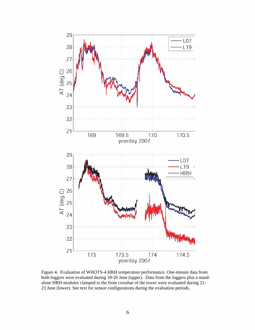
variables other than AT were within expected tolerances. The AT records (Figure 4, upper) were typically within 0.2°C during the day, but did not “track” well at high frequencies and showed differences of 0.4 to 0.6°C overnight. No obvious relationship was found between the AT difference and any other meteorological variable.

Between 20 and 23 June a series of overnight tests were performed which included a

stand-alone HRH module clamped to the front face of the tower top on the “port” side (closest to the L07 HRH module). During the first period (yearday = 172.8 – 173.7) the sensor configuration was L07 = HRH 218, L19 = HRH 219, stand-alone = HRH 504. Overnight differences between L07 and L09 were similar to those observed previously, while HRH 504 was within 0.1°C of L07 throughout, and faithfully tracked high-frequency variability (Figure 4, lower). During the second period (yearday = 173.9 – 174.7), L19 and the stand-alone were swapped, so that L19 = HRH 504 and stand-alone = HRH 219. Performance of L19 in this configuration was particularly poor, with persistent differences of 2°C from L07 (Figure 4, lower). HRH 219 operating as a stand-alone showed differences of 0.2 to 0.4°C.

It seemed that the temperature discrepancy followed the logger and/or the location, rather than the sensor. Since the RH values being logged on L19 looked fine, location was left as the most likely explanation. In addition, it seemed that HRH 504 had malfunctioned. Time had run out for further in-port testing, so the system was returned to its original configuration with the expectation that night time AT discrepancies would be reduced when the buoy was in open water.

6

Figure 4. Evaluation of WHOTS-4 HRH temperature performance. One-minute data from both loggers were evaluated during 18-20 June (upper). Data from the loggers plus a stand-alone HRH modules clamped to the front crossbar of the tower were evaluated during 21-23 June (lower). See text for sensor configurations during the evaluation periods.

7

A series of “sensor function checks,” including filling and draining the PRC modules, covering and uncovering the solar modules, and dunking the STC modules in a salt-water bucket, were done during the in-port evaluation period. The results of these checks, and a final in-port evaluation of hourly Argos data, showed all modules to be functioning as expected, with the exception of overnight AT differences of ~0.5°C, as described above. d. AutoIMET system on the Kilo Moana

The AutoIMET system was developed at WHOI to meet the need for improved marine meteorological observations from volunteer observing ships (VOS). AutoIMET is based on the ASIMET sensor suite and electronics, with the principal differences being a more compact physical configuration and the ability to interface with the NOAA Shipboard Environmental Acquisition System (SEAS). For WHOTS-4, an AutoIMET system was installed on the Kilo Moana to supplement the shipboard meteorological system. This differed from a typical VOS installation in three ways. First, a sea surface temperature sensor was not included; the ship’s Thermosalinograph was used instead. Second, data were transferred over the ship’s network from the data acquisition computer to another computer in the science lab, rather than being relayed from the acquisition computer to NOAA via Inmarsat. Third the sample interval on the acquisition computer was reduced from 6 min, typical for VOS, to 2 min (the AutoIMET logger records at 1 min intervals).

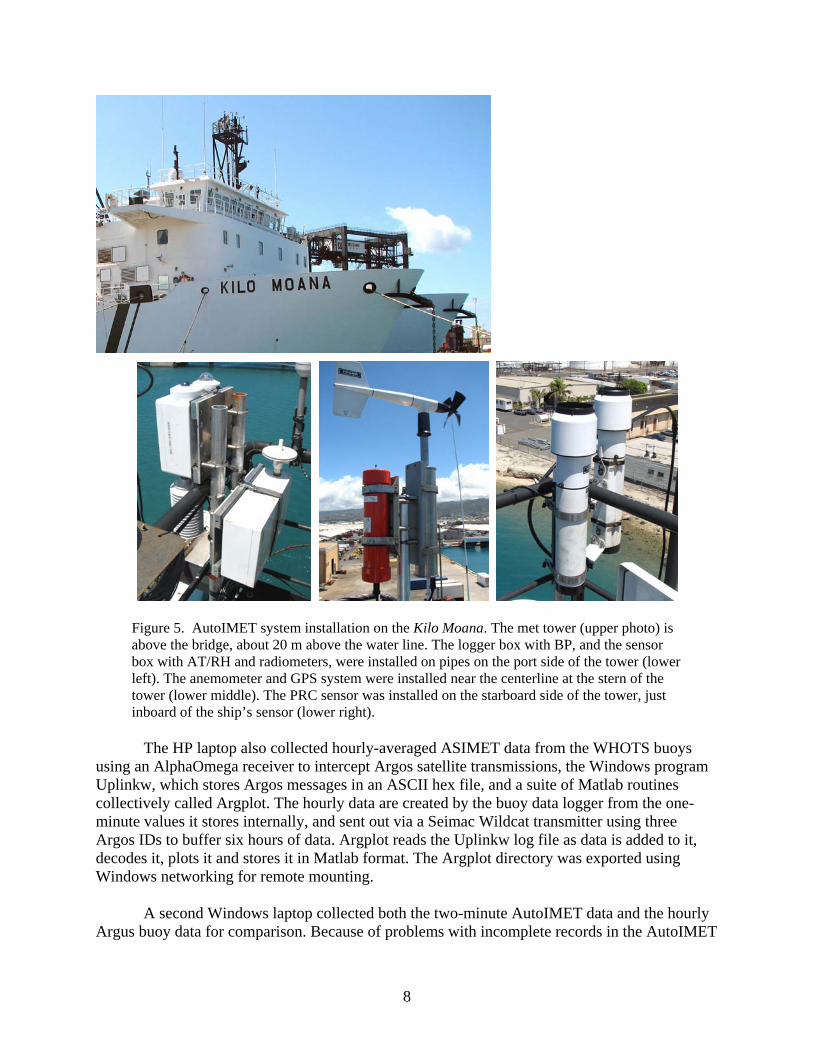
The AutoIMET configuration on Kilo Moana included five main components mounted

on the Kilo Moana science mast (Figure 5): a splash-proof housing with sensors for AT/RH, SWR and LWR, a second housing with a BP sensor and central data logger, a rain gauge, a wind sensor, and a GPS logger. The two housings were mounted on opposite sides of parallel pipe sections with the AT/RH sensor outboard and the radiometers in a location that minimized shadowing. The wind sensor and GPS logger were mounted back to back on a pipe extending from the stern rail of the mast, higher than the ship’s anemometers. The rain gauge was mounted on the starboard rail, adjacent to the ship’s rain gauge. According to the Kilo Moana Marine Technicians, the upper rail of the science mast is at 68 ft (20.7 m) above the water line. Measurements of the AutoIMET locations relative to the upper rail indicated that sensor heights were approximately 22 m for wind and 21 m for the rest of the sensors.

Data from the AutoIMET system were made available in real-time in the science lab,

using multiple laptop computers and the ship’s network, in order to assess performance of the WHOTS buoys relative to the ship (the GPS system logged internally, providing position data for post-cruise correction of the relative winds). AutoIMET data recorded by the central logger were captured by a data acquisition computer housed temporarily in the ship’s chart room. This computer, a Linux PC running Ubuntu, stored two-minute data records in hourly files, and also wrote out a cumulative data file that included all the data.

The first data processing computer, an HP laptop running Windows, used a secure shell

(ssh) command within Cygwin (a Windows shell program) to run a script on the data acquisition computer. This script (catmet.sh) first obtained the cumulative AutoIMET data file all_ai.txt, then begin a loop looking for a new hourly file. When a new file was found, the next-to-newest one would be returned. The returned data were piped through another script to reformat the data for Matlab, producing a file containing 2-minute data ready for the next stage of processing.

8

Figure 5. AutoIMET system installation on the Kilo Moana. The met tower (upper photo) is above the bridge, about 20 m above the water line. The logger box with BP, and the sensor box with AT/RH and radiometers, were installed on pipes on the port side of the tower (lower left). The anemometer and GPS system were installed near the centerline at the stern of the tower (lower middle). The PRC sensor was installed on the starboard side of the tower, just inboard of the ship’s sensor (lower right).

The HP laptop also collected hourly-averaged ASIMET data from the WHOTS buoys

using an AlphaOmega receiver to intercept Argos satellite transmissions, the Windows program Uplinkw, which stores Argos messages in an ASCII hex file, and a suite of Matlab routines collectively called Argplot. The hourly data are created by the buoy data logger from the one-minute values it stores internally, and sent out via a Seimac Wildcat transmitter using three Argos IDs to buffer six hours of data. Argplot reads the Uplinkw log file as data is added to it, decodes it, plots it and stores it in Matlab format. The Argplot directory was exported using Windows networking for remote mounting.

A second Windows laptop collected both the two-minute AutoIMET data and the hourly Argus buoy data for comparison. Because of problems with incomplete records in the AutoIMET

9

files, a Cygwin script was run to check record lengths of the incoming data, creating a local copy of the file which Matlab could easily load. A set of Matlab routines collectively called Vosplot loaded the local copy of the AutoIMET met data and generated hourly averages, centered on the half-hour to correspond with the Argos averages. Averaged AutoIMET data were listed to the laptop monitor and plotted. Matlab files containing the Argos data were then loaded from the HP running Argplot, accessed as a remote drive under Windows, and overplotted with the AutoIMET data.

10

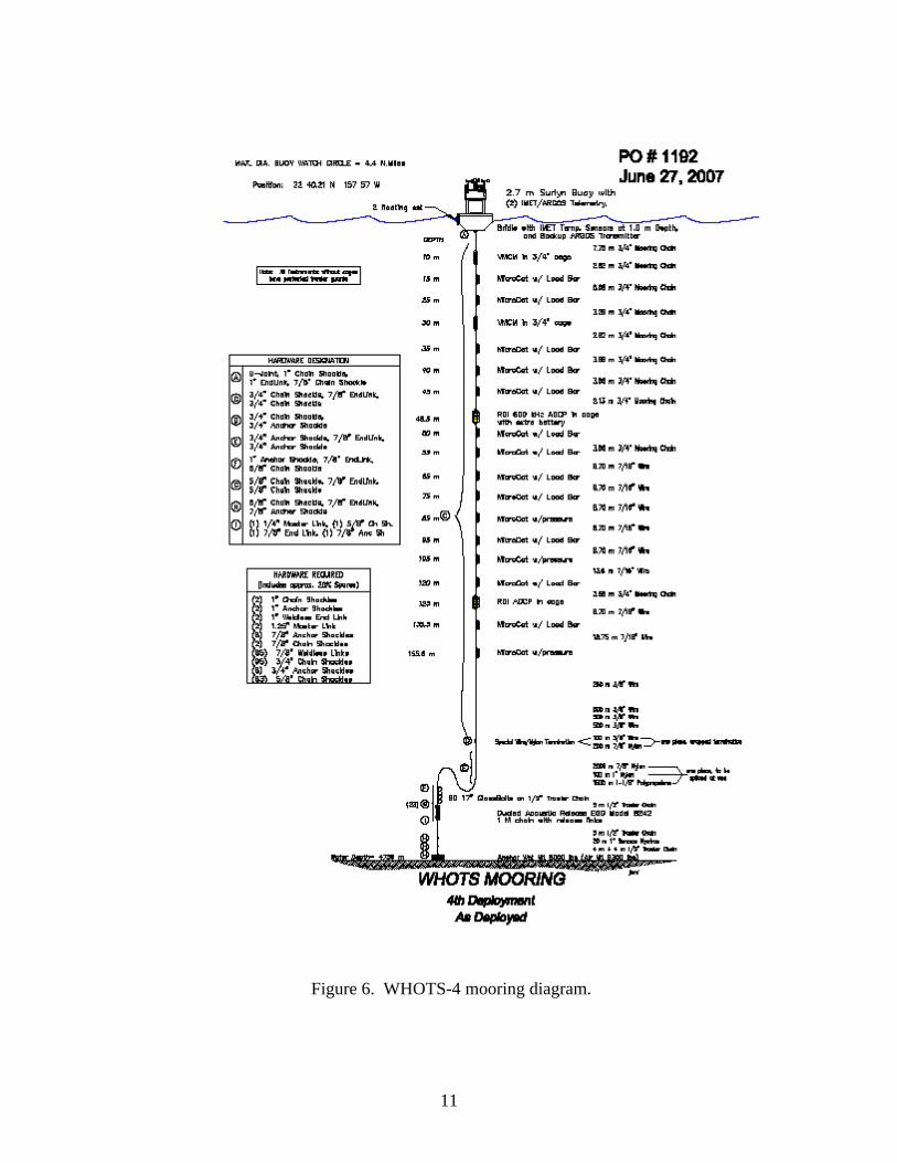
3. WHOTS-4 Mooring Description a. Mooring Design The mooring is an inverse catenary design utilizing wire rope, chain, nylon line and polypropylene line (Figure 6). The mooring scope (ratio of total mooring length to water depth) is about 1.25. The watch circle has a radius of approximately 2.2 nm (4.2 km). The surface element is a 2.7-meter diameter Surlyn foam buoy with a watertight electronics well and aluminum instrument tower. The two-layer foam buoy is “sandwiched” between aluminum top and bottom plates, and held together with eight 3/4" tie rods. The total buoy displacement is 16,000 pounds, with reserve buoyancy of approximately 12,000 lb when deployed in a typical configuration. The modular buoy design can be disassembled into components that will fit into a standard ISO container for shipment. A subassembly comprising the electronics well and meteorological instrument tower can be removed from the foam hull for ease of outfitting and testing of instrumentation. Two ASIMET data loggers and batteries sufficient to power the loggers and tower sensors for one year fit into the instrument well. Two complete sets of ASIMET sensor modules are attached to the upper section of the two-part aluminum tower at a height of about 3 m above the water line. The tower also contains a radar reflector, a marine lantern, and two independent Argos satellite transmission systems that provide continuous monitoring of buoy position. A third Argos positioning system was mounted within an access tube in the foam hull. This is a backup system, and would only be activated if the buoy capsized. For WHOTS-4, a self-contained Global Positioning System (GPS) receiver and a PCO2 sampling system were also mounted on the buoy. Sea surface temperature and salinity are measured by sensors bolted to the underside of the buoy hull and cabled to the loggers through an access tube through the buoy foam.

Fifteen temperature-conductivity sensors, two Vector Measuring Current Meters (VMCMs) and two Acoustic Doppler Current Meters (ADCP) were attached along the mooring using a combination of load cages (attached in-line between chain sections) and load bars. All instrumentation was along the upper 155 m of the mooring line (Figure 6). Dual acoustic releases, attached to a central load-bar, were placed approximately 33 m above the anchor. Above the release were eighty 17” glass balls meant to keep the release upright and ensure separation from the anchor after the release is fired. This flotation is sufficient for backup recovery, raising the lower end of the mooring to the surface in the event that surface buoyancy is lost.

11

Figure 6. WHOTS-4 mooring diagram.

12

b. Bird Barrier WHOTS-4 incorporates Nixalite Premium Bird Barrier Strips Model S as a physical

deterrence for pest birds and their accompanying guano deposition (Figure 7). The anti-bird wire is constructed of 316 stainless steel and is 4 inches high and 4 inches wide and has no less than 120 wire points per foot with full 180-degree coverage. The wire strips were installed fully around the crash bar, the flat top portion, inside lip, and carefully around the solars. Individual strips were 4 foot long and secured with cable ties. Order: S Kit 6 - 4 ft strips 24ft and S Kit 10 - 4ft strips 40ft Kit. The wires are sharp so it is recommended that gloves and eye protection be used for installation. Furthermore, transparent monofilament fishing line was installed in a simple X pattern inside the tower to also serve as a deterrent.

Figure 7: Bird Barrier

c. Anti-foul Treatment E-Paint’s products have been refined to best suit the wishes of WHOI- effective products

that remain relatively safe to apply. Treatment of the WHOTS-4 mooring was straightforward.

The Surlyn foam buoy hull and bottom plate were treated with E-Paint Sunwave +. Six coats (2.5 gallons) of paint were applied to the foam hull, and two coats were applied to the bottom plate and universal joint.

E-Paint ZO was used to coat the two SBE 37s mounted to the bottom of the buoy, and on the floating SST and SST bracket. Two coats of ZO were used on these components.

E-Paint ZO was also used to treat the instruments mounted on the mooring line down to 50 meters. The shield over the conductivity cell on SBE 37s and SBE 16s was coated on both sides. The conductivity cell was coated as well. On the VMCMs, propellers were treated with E-Paint. VMCM stings were painted with E-Paint ZO prior to deployment.

Paint on WHOTS 4 hull. One new coat of E-prime 1000 on foam --- existing paint/primer on bottom plate.

four heavy coats of Sunwave on hull. Two coats on bottom. Also sprayed the bottom with a can of the Interlux Trilux prop and outdrive paint (one coat)

Floating SST frame and floater had two coats of Interlux Trilux prop and outdrive paint.

13

d. Buoy Instrumentation

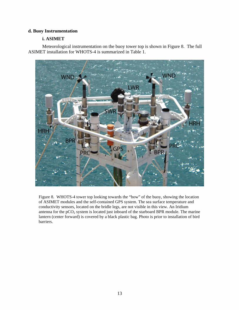
i. ASIMET Meteorological instrumentation on the buoy tower top is shown in Figure 8. The full ASIMET installation for WHOTS-4 is summarized in Table 1.

Figure 8. WHOTS-4 tower top looking towards the “bow” of the buoy, showing the location of ASIMET modules and the self-contained GPS system. The sea surface temperature and conductivity sensors, located on the bridle legs, are not visible in this view. An Iridium antenna for the pCO2 system is located just inboard of the starboard BPR module. The marine lantern (center forward) is covered by a black plastic bag. Photo is prior to installation of bird barriers.

14

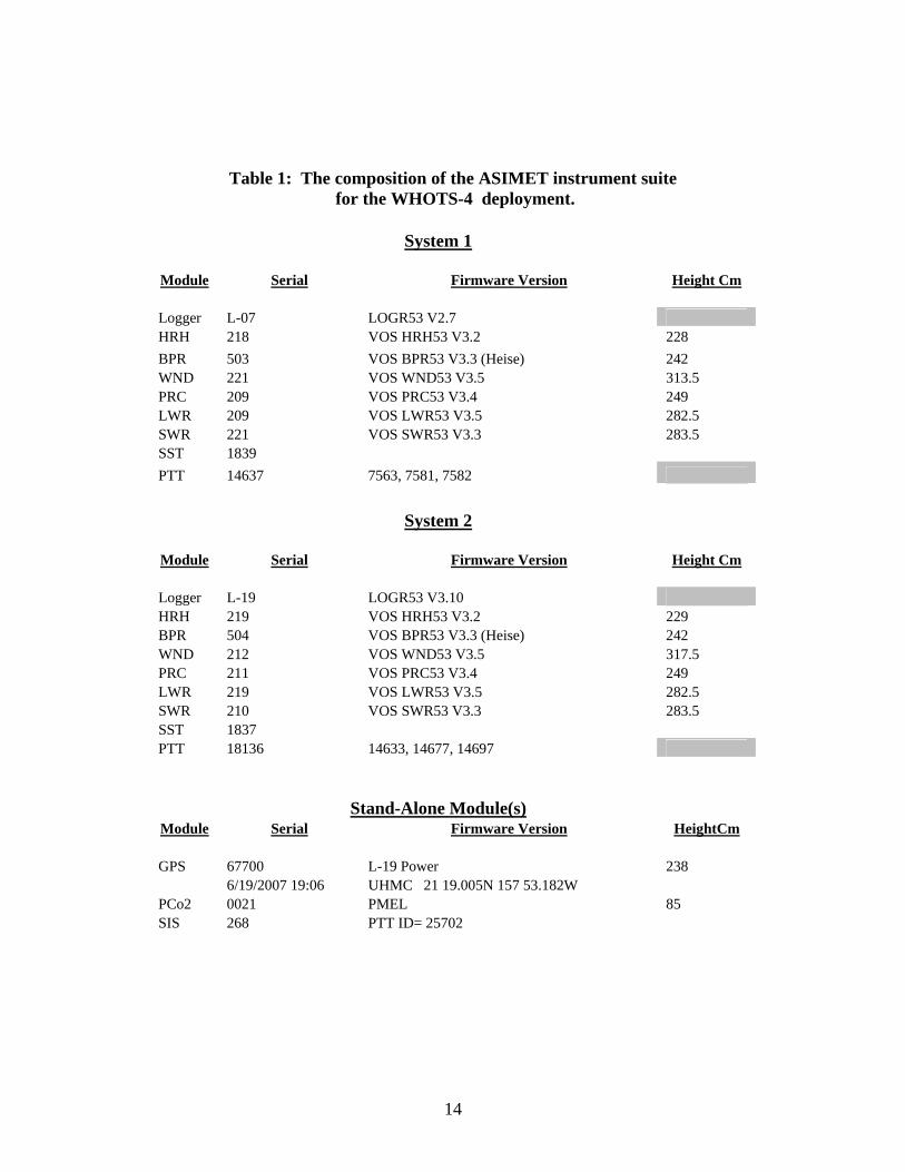
Table 1: The composition of the ASIMET instrument suite for the WHOTS-4 deployment.

System 1 Module Serial Firmware Version Height Cm Logger L-07 LOGR53 V2.7 HRH 218 VOS HRH53 V3.2 228 BPR 503 VOS BPR53 V3.3 (Heise) 242 WND 221 VOS WND53 V3.5 313.5 PRC 209 VOS PRC53 V3.4 249 LWR 209 VOS LWR53 V3.5 282.5 SWR 221 VOS SWR53 V3.3 283.5 SST 1839 PTT 14637 7563, 7581, 7582 System 2 Module Serial Firmware Version Height Cm Logger L-19 LOGR53 V3.10 HRH 219 VOS HRH53 V3.2 229 BPR 504 VOS BPR53 V3.3 (Heise) 242 WND 212 VOS WND53 V3.5 317.5 PRC 211 VOS PRC53 V3.4 249 LWR 219 VOS LWR53 V3.5 282.5 SWR 210 VOS SWR53 V3.3 283.5 SST 1837 PTT 18136 14633, 14677, 14697 Stand-Alone Module(s) Module Serial Firmware Version HeightCm GPS 67700 L-19 Power 238 6/19/2007 19:06 UHMC 21 19.005N 157 53.182W PCo2 0021 PMEL 85 SIS 268 PTT ID= 25702

15

ii. Floating SST Furthermore, the floating SST was modified to incorporate a redundant sensor. The

WHOTS-4 floating SST consists of a Brancker TR-1050 appendage in addition to the standard Seabird SBE 39.

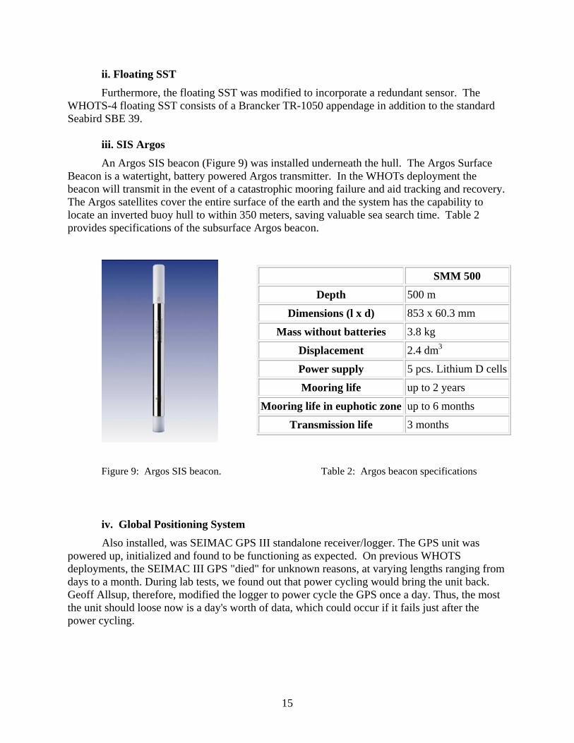
iii. SIS Argos An Argos SIS beacon (Figure 9) was installed underneath the hull. The Argos Surface

Beacon is a watertight, battery powered Argos transmitter. In the WHOTs deployment the beacon will transmit in the event of a catastrophic mooring failure and aid tracking and recovery. The Argos satellites cover the entire surface of the earth and the system has the capability to locate an inverted buoy hull to within 350 meters, saving valuable sea search time. Table 2 provides specifications of the subsurface Argos beacon.

Figure 9: Argos SIS beacon. Table 2: Argos beacon specifications

iv. Global Positioning System Also installed, was SEIMAC GPS III standalone receiver/logger. The GPS unit was powered up, initialized and found to be functioning as expected. On previous WHOTS deployments, the SEIMAC III GPS "died" for unknown reasons, at varying lengths ranging from days to a month. During lab tests, we found out that power cycling would bring the unit back. Geoff Allsup, therefore, modified the logger to power cycle the GPS once a day. Thus, the most the unit should loose now is a day's worth of data, which could occur if it fails just after the power cycling.

SMM 500

Depth 500 m

Dimensions (l x d) 853 x 60.3 mm

Mass without batteries 3.8 kg

Displacement 2.4 dm3

Power supply 5 pcs. Lithium D cells

Mooring life up to 2 years

Mooring life in euphotic zone up to 6 months

Transmission life 3 months

16

v. Telemetry With regards to telemetry, WHOTS4 was equipped with 2 Argos transmitting systems.

Argos functioned as expected. vi. pC02

The WHOI Hawaii Ocean Time-series Station (WHOTS) is located near the HOT shipboard time series site (22.75°N, 158°W) in order to maximize the utility of both data sets. There are several advantages of this site. These include: (1) A rich historical database is available for the site; this is useful for setting up new moored instruments, as well as facilitating intercomparisons and interpretations, (2) The HOT site is well away from sources of anthropogenic influence, which is especially important for trace metal, dissolved CO2, oligotrophic biological and optical, and aerosol studies, (3) The ongoing JGOFS time-series sampling program (approximately monthly frequency) collects a relatively complete suite of physical, chemical (including nutrients and CO2), and biological data. There are analogous advantages for comparisons and calibrations of present and emerging sensors, 3) Remote sensing data (SeaWiFS, AVHRR, TOPEX/Poseidon and ERS-series altimetry, QuikScat, MODIS, and weather images) are collected, thus providing complementary measurements for our study and vice versa, (4) There is a documented need for high temporal resolution/mooring data at the site because of undersampling and aliasing as described above, (5) There is a reasonably high probability of passage of intense storms and occasionally hurricanes, (6) Other testing is either ongoing or planned from other platforms near the HOT site (e.g., AUVs), and (7) The region is often used for other scientific studies that can be used to enhance the HOT and WHOTS data sets and vice versa.

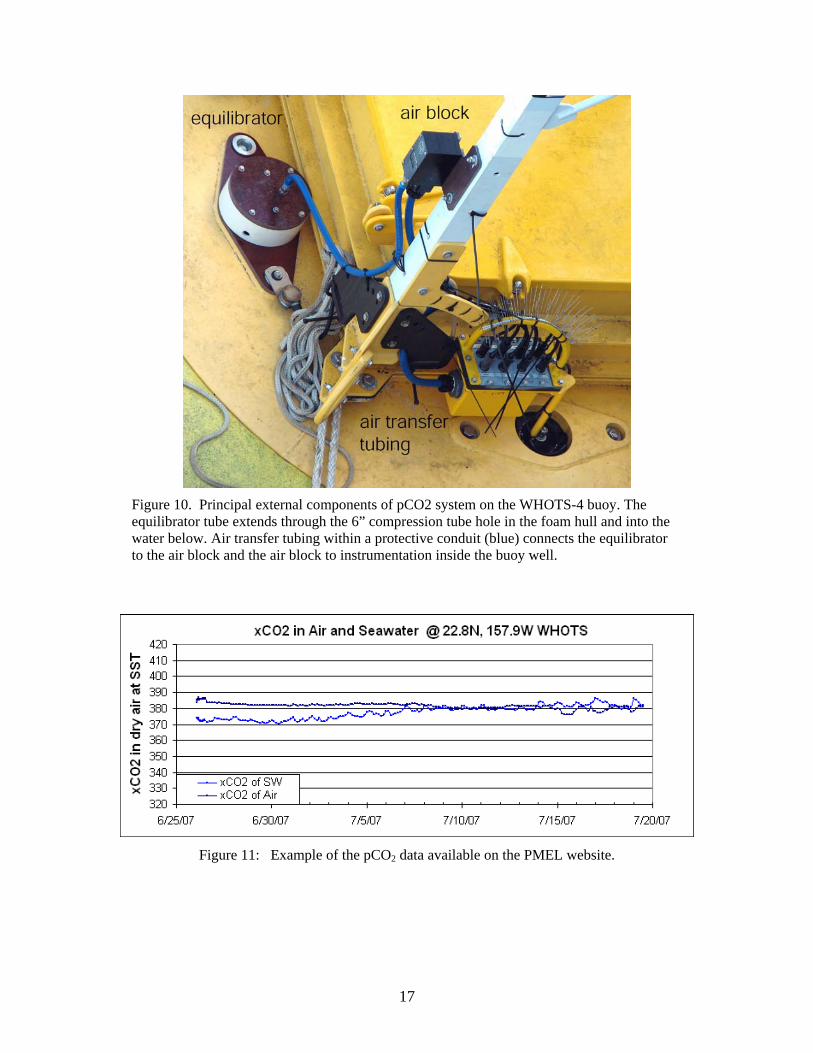
Adding a pCO2 system to the WHOTS mooring expands the OceanSITES moored pCO2 network. The current network is developing in the North Pacific. This site provides the next logical step for an expansion. CO2 measurements are made every three hours in marine boundary layer air and air equilibrated with surface seawater using an infra-red detector. The detector is calibrated prior to each reading using a zero gas derived by chemically stripping CO2 from a closed loop of air and a span gas (470 ppm CO2) produced and calibrated by NOAA's Earth System Research Laboratory (ESRL). For an overview of the system visit: http://www.pmel.noaa.gov/co2/moorings/eq_pco2/pmelsys.htm. PMEL pCO2 system 0021 was used for this deployment. The external components of the pCO2 installation for WHOTS-4 are shown in Figure 10. A summary file of the measurements is transmitted once per day and plots of the data are posted in near real-time to the web (Figure 11). To view the daily data visit the NOAA PMEL Moored CO2 Website: http://www.pmel.noaa.gov/co2/moorings/hot/hot_main.htm. Within a year of system recovery, the final processed data are submitted to the Carbon Dioxide Information Analysis Center (CDIAC) for release to the public.

17

Figure 10. Principal external components of pCO2 system on the WHOTS-4 buoy. The equilibrator tube extends through the 6” compression tube hole in the foam hull and into the water below. Air transfer tubing within a protective conduit (blue) connects the equilibrator to the air block and the air block to instrumentation inside the buoy well.

Figure 11: Example of the pCO2 data available on the PMEL website.

18

e. Subsurface Instrumentation

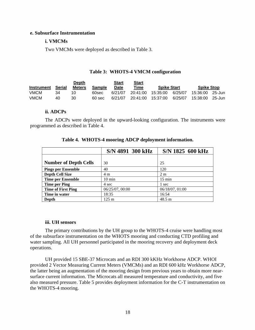
i. VMCMs Two VMCMs were deployed as described in Table 3.

Table 3: WHOTS-4 VMCM configuration

Instrument Serial Depth Meters Sample

Start Date

Start Time Spike Start Spike Stop

VMCM 34 10 60sec 6/21/07 20:41:00 15:35:00 6/25/07 15:36:00 25-Jun VMCM 40 30 60 sec 6/21/07 20:41:00 15:37:00 6/25/07 15:38:00 25-Jun

ii. ADCPs The ADCPs were deployed in the upward-looking configuration. The instruments were programmed as described in Table 4.

Table 4. WHOTS-4 mooring ADCP deployment information.

S/N 4891 300 kHz S/N 1825 600 kHz

Number of Depth Cells 30

25

Pings per Ensemble 40 120 Depth Cell Size 4 m 2 m Time per Ensemble 10 min 15 min Time per Ping 4 sec 1 sec Time of First Ping 06/25/07, 00:00 06/18/07, 01:00 Time in water 18:35 16:54 Depth 125 m 48.5 m

iii. UH sensors The primary contributions by the UH group to the WHOTS-4 cruise were handling most of the subsurface instrumentation on the WHOTS mooring and conducting CTD profiling and water sampling. All UH personnel participated in the mooring recovery and deployment deck operations.

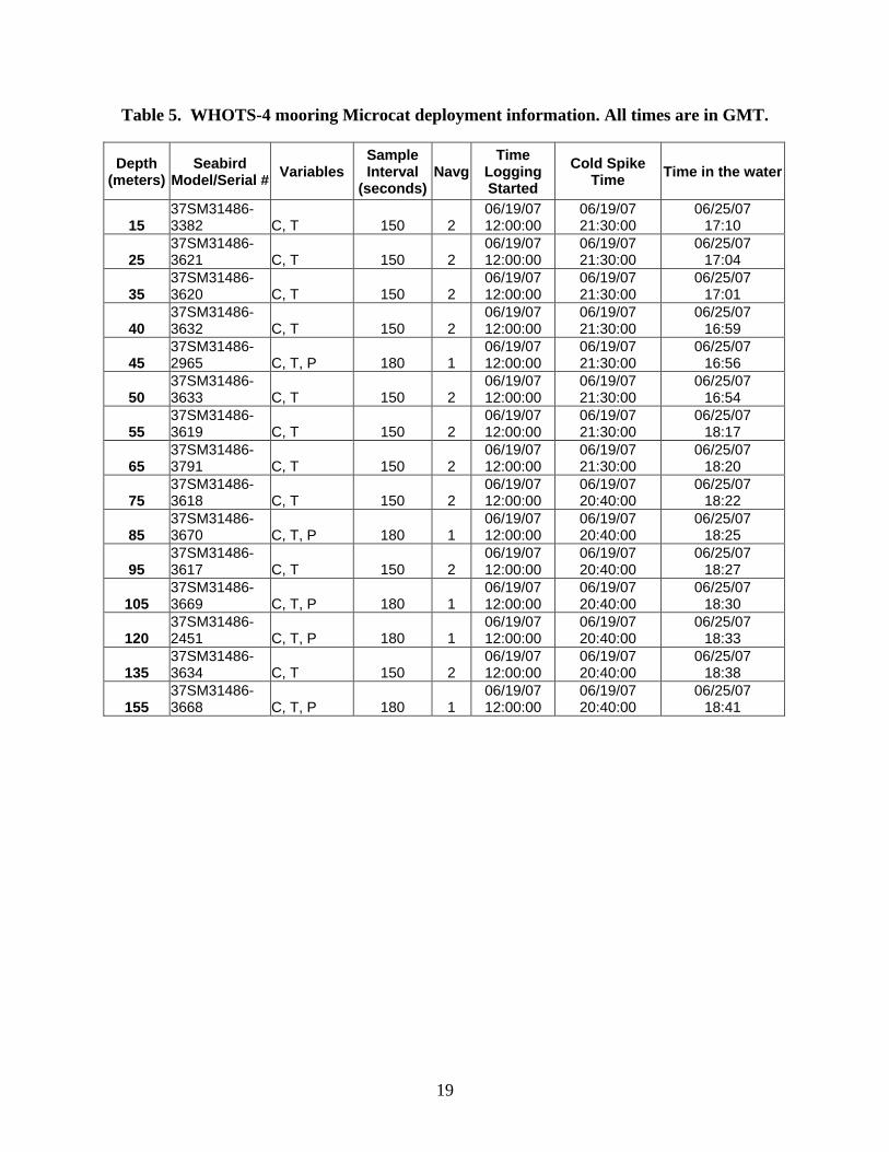
UH provided 15 SBE-37 Microcats and an RDI 300 kKHz Workhorse ADCP. WHOI provided 2 Vector Measuring Current Meters (VMCMs) and an RDI 600 kHz Workhorse ADCP, the latter being an augmentation of the mooring design from previous years to obtain more near-surface current information. The Microcats all measured temperature and conductivity, and five also measured pressure. Table 5 provides deployment information for the C-T instrumentation on the WHOTS-4 mooring.

19

Table 5. WHOTS-4 mooring Microcat deployment information. All times are in GMT.

Depth (meters)

Seabird Model/Serial # Variables

Sample Interval

(seconds)Navg

Time Logging Started

Cold Spike Time Time in the water

15 37SM31486-3382 C, T 150 2

06/19/07 12:00:00

06/19/07 21:30:00

06/25/07 17:10

25 37SM31486-3621 C, T 150 2

06/19/07 12:00:00

06/19/07 21:30:00

06/25/07 17:04

35 37SM31486-3620 C, T 150 2

06/19/07 12:00:00

06/19/07 21:30:00

06/25/07 17:01

40 37SM31486-3632 C, T 150 2

06/19/07 12:00:00

06/19/07 21:30:00

06/25/07 16:59

45 37SM31486-2965 C, T, P 180 1

06/19/07 12:00:00

06/19/07 21:30:00

06/25/07 16:56

50 37SM31486-3633 C, T 150 2

06/19/07 12:00:00

06/19/07 21:30:00

06/25/07 16:54

55 37SM31486-3619 C, T 150 2

06/19/07 12:00:00

06/19/07 21:30:00

06/25/07 18:17

65 37SM31486-3791 C, T 150 2

06/19/07 12:00:00

06/19/07 21:30:00

06/25/07 18:20

75 37SM31486-3618 C, T 150 2

06/19/07 12:00:00

06/19/07 20:40:00

06/25/07 18:22

85 37SM31486-3670 C, T, P 180 1

06/19/07 12:00:00

06/19/07 20:40:00

06/25/07 18:25

95 37SM31486-3617 C, T 150 2

06/19/07 12:00:00

06/19/07 20:40:00

06/25/07 18:27

105 37SM31486-3669 C, T, P 180 1

06/19/07 12:00:00

06/19/07 20:40:00

06/25/07 18:30

120 37SM31486-2451 C, T, P 180 1

06/19/07 12:00:00

06/19/07 20:40:00

06/25/07 18:33

135 37SM31486-3634 C, T 150 2

06/19/07 12:00:00

06/19/07 20:40:00

06/25/07 18:38

155 37SM31486-3668 C, T, P 180 1

06/19/07 12:00:00

06/19/07 20:40:00

06/25/07 18:41

20

4. WHOTS-4 Mooring Deployment

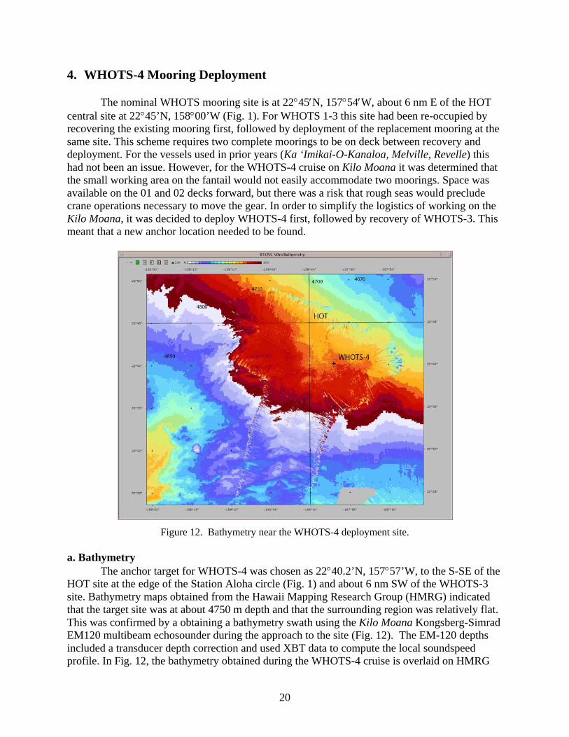
The nominal WHOTS mooring site is at 22°45′N, 157°54′W, about 6 nm E of the HOT central site at 22°45’N, 158°00’W (Fig. 1). For WHOTS 1-3 this site had been re-occupied by recovering the existing mooring first, followed by deployment of the replacement mooring at the same site. This scheme requires two complete moorings to be on deck between recovery and deployment. For the vessels used in prior years (Ka ‘Imikai-O-Kanaloa, Melville, Revelle) this had not been an issue. However, for the WHOTS-4 cruise on Kilo Moana it was determined that the small working area on the fantail would not easily accommodate two moorings. Space was available on the 01 and 02 decks forward, but there was a risk that rough seas would preclude crane operations necessary to move the gear. In order to simplify the logistics of working on the Kilo Moana, it was decided to deploy WHOTS-4 first, followed by recovery of WHOTS-3. This meant that a new anchor location needed to be found.

Figure 12. Bathymetry near the WHOTS-4 deployment site.

a. Bathymetry

The anchor target for WHOTS-4 was chosen as 22°40.2’N, 157°57’W, to the S-SE of the HOT site at the edge of the Station Aloha circle (Fig. 1) and about 6 nm SW of the WHOTS-3 site. Bathymetry maps obtained from the Hawaii Mapping Research Group (HMRG) indicated that the target site was at about 4750 m depth and that the surrounding region was relatively flat. This was confirmed by a obtaining a bathymetry swath using the Kilo Moana Kongsberg-Simrad EM120 multibeam echosounder during the approach to the site (Fig. 12). The EM-120 depths included a transducer depth correction and used XBT data to compute the local soundspeed profile. In Fig. 12, the bathymetry obtained during the WHOTS-4 cruise is overlaid on HMRG

21

regional synthesis bathymetry (http://www.soest.hawaii.edu/HMRG/multibeam/index.html). The nominal WHOTS mooring design was for a depth of 4700 m ±100 m. The EM-120 depth at the anchor target was 4756 m, and the survey indicated that depth variability within about 2 nm of the anchor site was ± 20 m. Thus, no adjustment to the mooring design was necessary. b. Deployment Approach

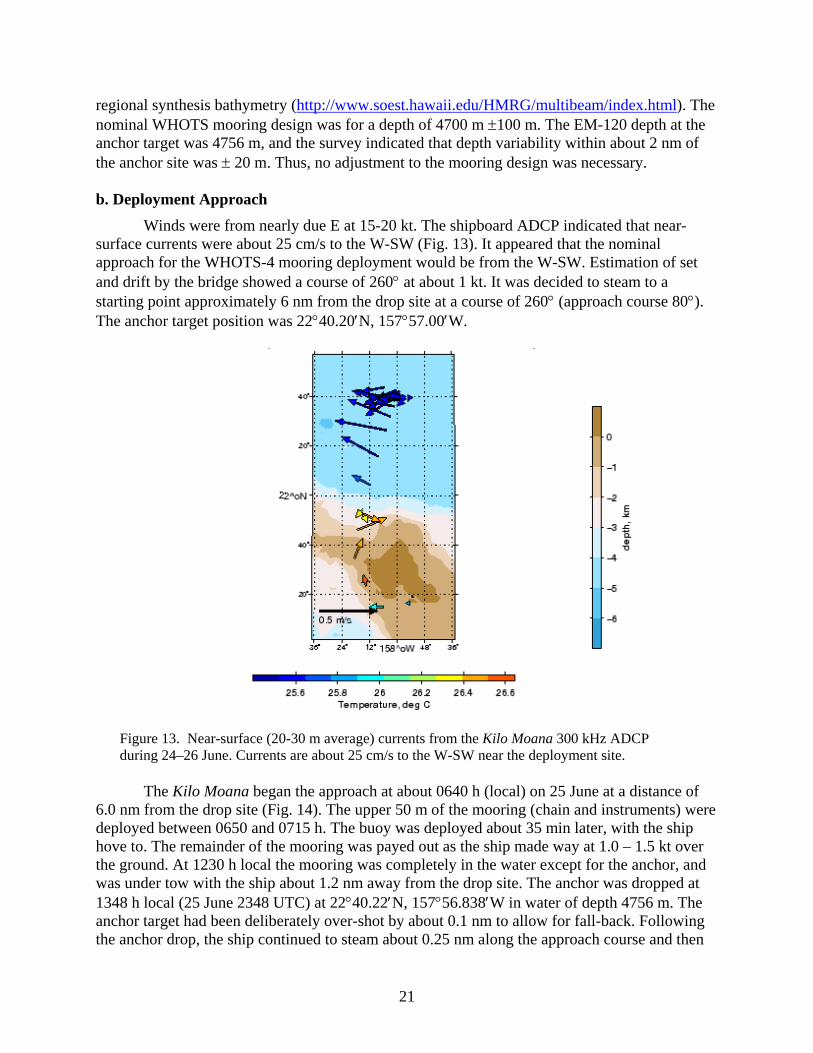
Winds were from nearly due E at 15-20 kt. The shipboard ADCP indicated that near-surface currents were about 25 cm/s to the W-SW (Fig. 13). It appeared that the nominal approach for the WHOTS-4 mooring deployment would be from the W-SW. Estimation of set and drift by the bridge showed a course of 260° at about 1 kt. It was decided to steam to a starting point approximately 6 nm from the drop site at a course of 260° (approach course 80°). The anchor target position was 22°40.20′N, 157°57.00′W.

Figure 13. Near-surface (20-30 m average) currents from the Kilo Moana 300 kHz ADCP during 24–26 June. Currents are about 25 cm/s to the W-SW near the deployment site.

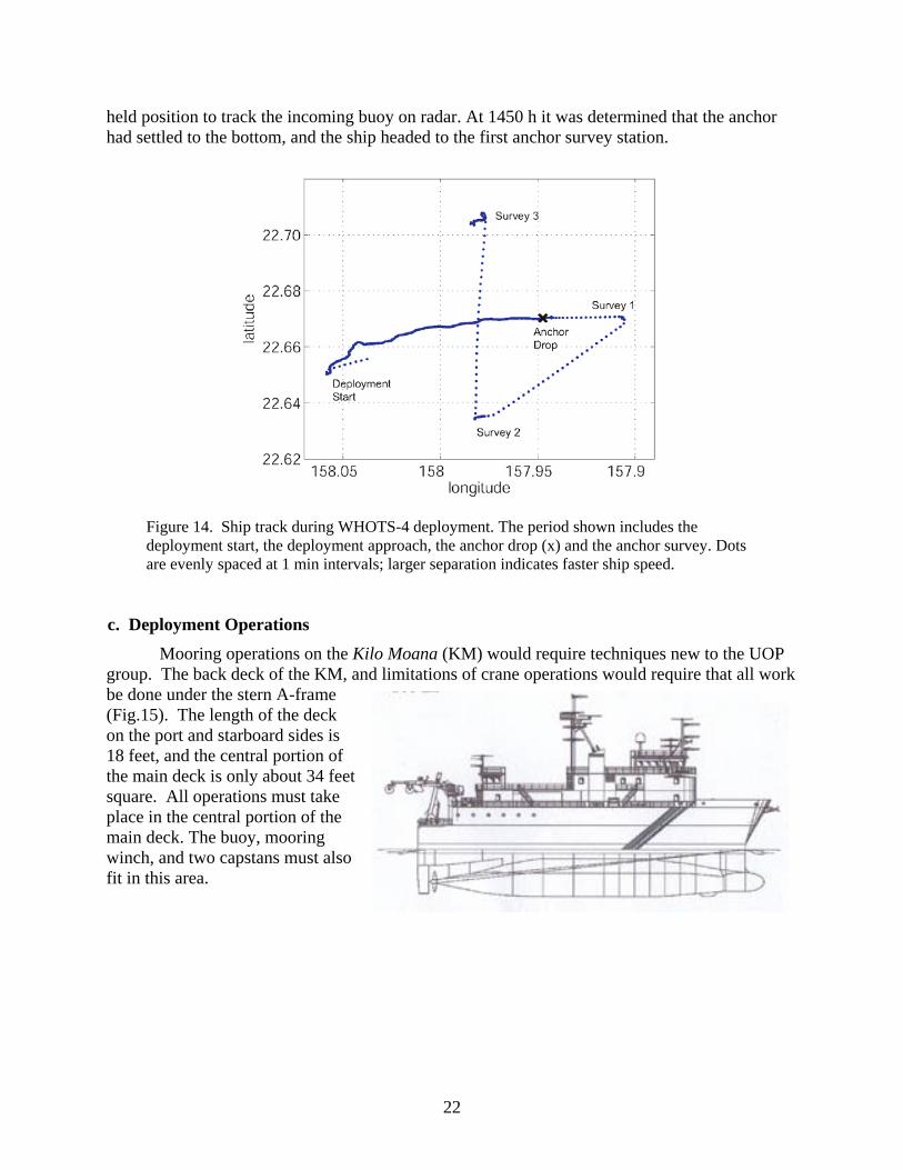
The Kilo Moana began the approach at about 0640 h (local) on 25 June at a distance of

6.0 nm from the drop site (Fig. 14). The upper 50 m of the mooring (chain and instruments) were deployed between 0650 and 0715 h. The buoy was deployed about 35 min later, with the ship hove to. The remainder of the mooring was payed out as the ship made way at 1.0 – 1.5 kt over the ground. At 1230 h local the mooring was completely in the water except for the anchor, and was under tow with the ship about 1.2 nm away from the drop site. The anchor was dropped at 1348 h local (25 June 2348 UTC) at 22°40.22′N, 157°56.838′W in water of depth 4756 m. The anchor target had been deliberately over-shot by about 0.1 nm to allow for fall-back. Following the anchor drop, the ship continued to steam about 0.25 nm along the approach course and then

22

held position to track the incoming buoy on radar. At 1450 h it was determined that the anchor had settled to the bottom, and the ship headed to the first anchor survey station.

Figure 14. Ship track during WHOTS-4 deployment. The period shown includes the deployment start, the deployment approach, the anchor drop (x) and the anchor survey. Dots are evenly spaced at 1 min intervals; larger separation indicates faster ship speed.

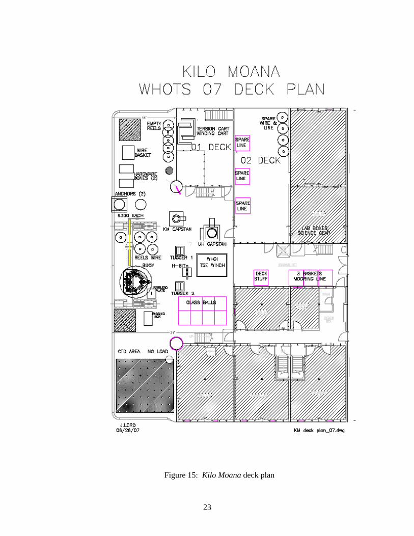
c. Deployment Operations Mooring operations on the Kilo Moana (KM) would require techniques new to the UOP

group. The back deck of the KM, and limitations of crane operations would require that all work be done under the stern A-frame (Fig.15). The length of the deck on the port and starboard sides is 18 feet, and the central portion of the main deck is only about 34 feet square. All operations must take place in the central portion of the main deck. The buoy, mooring winch, and two capstans must also fit in this area.

23

Figure 15: Kilo Moana deck plan

24

The setup for the mooring deployment included running a Spectra working line through

the turning blocks on the A-frame, and over the flag block in the center of the A-frame. A Gifford block was shackled to the working line under the A-frame, and the ship’s capstan was used to haul the block up and suspend it just below the flag block. The A-frame was positioned so the block hung slightly aft of the transom. The working end of the Spectra was stopped off on a cleat. An air tugger was positioned about 15 feet forward of the stern on the port side of the A-frame. The end of the tugger line was fitted with a ¾” chain hook.

Instruments from the surface to 50 meters were pre-rigged with chain and hardware at the top of the load bar or instrument cage. Instruments below 50 meters were pre rigged with wire rope or chain shots shackled to the bottom of the load bar or cage. Doing this work in advance saved time during the actual deployment process.

To begin the mooring deployment a shot of wire rope was passed from the mooring winch through the Gifford block and lowered to the deck. A 150-meter Spectra working line was shackled to the bottom of the 50-meter MicroCat load bar. The top of the 50-meter MicroCat load bar was shackled directly into the cage of the 48.5-meter ADCP. The working wire from the winch was shackled into a link at the top of a 2.13 meter shot of 3/4” chain connected to the top of the ADCP cage. To begin the deployment the winch hauled in wire to suspend the chain, ADCP, and MicroCat from the A-Frame. Next, the winch payed out wire to lower the instruments and chain to the water. A person tending the 150-meter working line on a cleat payed out line approximately equal to what was being lowered into the water.

When the top of the chain above the ADCP was about .5 meters above the transom, the tugger line with chain hook was attached to the chain and the tugger pulled the chain in to the deck. The winch lowered the chain to the deck and a backup stopper line was attached to the link on the chain before disconnecting from the winch line. The procedure for inserting the 45 meter MicroCat and the rest of the instruments above 50-meters included: shackling the bottom of the instrument cage or load bar into the link at the top of the instrument array suspended in the water, lifting the instrument and attached chain shot off the deck with the winch, paying out with the winch and Spectra working line, stopping off the chain, and repeating this process.

The 7.75 meter shot of chain above the 10 meter depth VMCM was stopped off using a pear link shackled into the chain about 2 meters from the top. A slip line was passed through the link and secured to a cleat. The port side crane was used to move the buoy from its position under the A-frame on the starboard side to a position generally centered under the A-frame. A 1” shackle was used to attach the top section of mooring chain to the buoy.

To prepare for the buoy deployment cleats were set up on each side of the buoy hull. Slip lines were passed through the handling rings on the buoy hull and secured. A “west coast” quick release was rigged to the buoy’s lifting bale, and attached to the working line on the A-frame. The ship was instructed to move ahead slowly. When all preparations for the deployment were complete, lines and straps securing the buoy were removed. The slip line holding the mooring tension was slowly removed and the mooring load was transferred to the buoy.

25

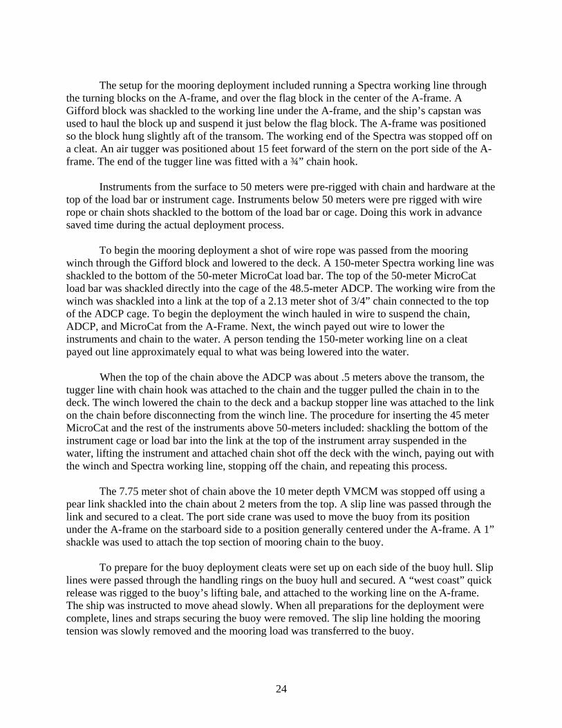
The buoy was lifted off the deck with the capstan and working line rigged to the A-frame. The A-frame was moved back, and slip lines kept the buoy in check as it moved out beyond the transom of the ship. When the A-frame was fully extended, the port slip line was removed. This allowed the buoy to spin 90 degrees and provide a better angle for the quick release line. The buoy was slowly lowered into the water, and once it settled in the quick release was tripped. The starboard slip line was slowly pulled free of the buoy as the ship moved away from it.

As the ship moved away from the buoy, more of the Spectra working line attached to the bottom of the mooring chain was payed out to keep the tension down. As the buoy settled in behind the ship and everything appeared stable, this working line was slackened and removed from the cleat. The end of this working line had been previously shackled to the mooring winch wire. The ship speed was reduced to just enough to provide steerage, and the winch was used to pull in the working line coming from the deployed mooring chain.

When the end of the working line and the bottom of the chain below the 50-meter MicroCat was pulled over the transom, stopper lines were attached to the link at the bottom of the chain. The working line was removed. The 55-meter MicroCat was moved into position and the bottom of the MicroCat load bar was shackled into the mooring chain. The bottom of the wire rope section was shackled into the wire on the winch. The winch hauled in on the wire until it had the load from the mooring. Stopper lines were slacked off and removed.

The winch payed out wire until the bottom end of end of the short shot of wire was about 1 meter above the deck, the winch stopped and stopper lines were attached to the link in the termination. The winch wire was lowered to the deck and removed, and the next instrument and wire shot was inserted into the line. The procedure continued until all instruments had been deployed.

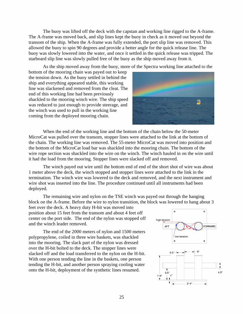
The remaining wire and nylon on the TSE winch was payed out through the hanging block on the A-frame. Before the wire to nylon transition, the block was lowered to hang about 3 feet over the deck. A heavy duty H-bit was moved into position about 15 feet from the transom and about 4 feet off center on the port side. The end of the nylon was stopped off and the winch leader removed.

The end of the 2000 meters of nylon and 1500 meters polypropylene, coiled in three wire baskets, was shackled into the mooring. The slack part of the nylon was dressed over the H-bit bolted to the deck. The stopper lines were slacked off and the load transferred to the nylon on the H-bit. With one person tending the line in the baskets, one person tending the H-bit, and another person spraying cooling water onto the H-bit, deployment of the synthetic lines resumed.

26

When the end of the polypropylene line was reached, payout was stopped and a Yale grip and stopper lines were used to take tension off the H-bit. The winch leader line was shackled into the end of the polypropylene line. The polypropylene line was removed from the H-bit. The winch line and mooring line were wound up taking the mooring tension away from the stopper lines on the Yale grip. The Yale grip and stopper lines were removed. The TSE winch payed out the mooring line until the thimble was approximately 2 meters from the ship’s transom. At this point, the hanging block was lowered to the deck and removed.

The next step was the deployment of 80 glass balls. The glass balls were bolted on 1/2”

trawler chain in four ball (4 meter) increments. The port crane was used to lift each string of glass balls out of the wire baskets and lower them to the deck. The first string of balls was dragged aft and connected to the end of the polypropylene line. The winch leader was then connected to the string of balls. The winch leader was pulled tight, and the stopper lines were eased out and disconnected. The winch payed out until 3 balls were beyond the transom. The two stopper lines were then attached to the link at the end of the string of balls. Another set of glass balls were then dragged into place and shackled into the mooring. This procedure continued until all 80 glass balls were attached to the mooring line. A five meter shot of ½” chain was shackled into the mooring and stopped off with approximately 2 meters of chain remaining on the deck.

At this point, the ship was still approximately 1.2 nm from the target drop position. The

ship towed the mooring toward the drop position in this configuration. Approximately 0.2 nm from the site, the final sections of the mooring were prepared. The tandem-mounted acoustic releases were shackled into the mooring chain at the transom. Another 5-meter shot of chain was attached to the bottom link on the dual release chain. This chain was then shackled into the 20-meter nylon anchor pennant, which was shackled into another four meters of ½” chain. The chain, anchor pennant, and next shot of chain were wound onto the winch. The stopper lines were removed.

The anchor, positioned on the port side, just outboard of the A-frame was rigged with a

4-meter shot of ½” chain. The bolts holding the anchor tip plate to the deck were removed. The chain lashings on the anchor were removed, and a expendable back stay was rigged on the anchor to secure it.

A ½” chain hook was shackled into the working line hanging from the A-frame and

hooked into the chain just below the acoustic releases. The working line was pulled up with the capstan, lifting the releases off the deck. The winch payed out and the A-frame was moved out until the releases were clear of the transom. The working line was lowered and the chain hook removed from the mooring. The winch continued to pay out until the 5-meter chain, 20-meter nylon, and 2 meters of the final 4-meter shot of chain had been deployed.

A sling link was shackled into the ½” chain about two meters up from the Sampson

anchor pennant. A slip line was passed through the link and secured to a cleat on the A-frame and another cleat on the deck. The section of chain from the anchor was shackled to the end of the chain on the mooring. The crane was positioned with the boom slightly aft of the lifting bridle on the tip plate. The crane was then attached to the tip plate bridle and slight tension was taken on the crane wire.

27

As the ship approached the launch site, the slip line was eased out and the mooring load

was transferred to the anchor. At the signal from the Chief Scientist, the backstay was cut, the crane wire was raised, and the tip plate raised enough to let the anchor slip into the water.

d. Anchor survey The anchor survey was done by acoustic ranging on one of the releases to determine the

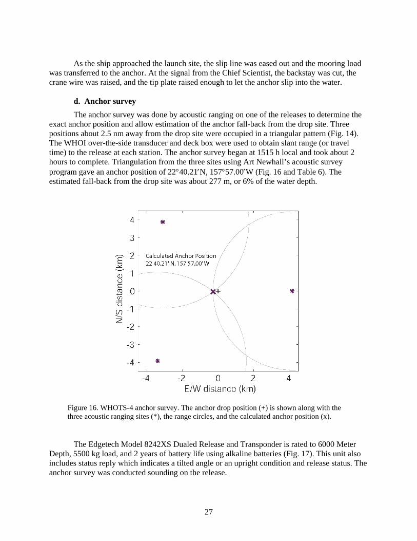
exact anchor position and allow estimation of the anchor fall-back from the drop site. Three positions about 2.5 nm away from the drop site were occupied in a triangular pattern (Fig. 14). The WHOI over-the-side transducer and deck box were used to obtain slant range (or travel time) to the release at each station. The anchor survey began at 1515 h local and took about 2 hours to complete. Triangulation from the three sites using Art Newhall’s acoustic survey program gave an anchor position of 22°40.21′N, 157°57.00′W (Fig. 16 and Table 6). The estimated fall-back from the drop site was about 277 m, or 6% of the water depth.

Figure 16. WHOTS-4 anchor survey. The anchor drop position (+) is shown along with the three acoustic ranging sites (*), the range circles, and the calculated anchor position (x).

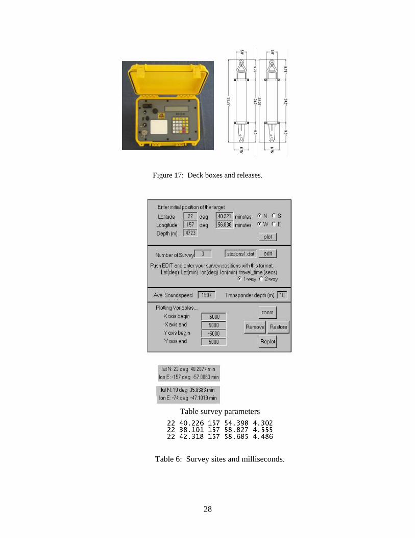
The Edgetech Model 8242XS Dualed Release and Transponder is rated to 6000 Meter Depth, 5500 kg load, and 2 years of battery life using alkaline batteries (Fig. 17). This unit also includes status reply which indicates a tilted angle or an upright condition and release status. The anchor survey was conducted sounding on the release.

28

Figure 17: Deck boxes and releases.

Table survey parameters

Table 6: Survey sites and milliseconds.

29

5. WHOTS-3 Mooring Recovery

a. Recovery Operations The WHOTS-3 mooring was recovered buoy-first rather than release-first in an effort to

make instruments available for data recovery as soon as possible, and to minimize the use of the workboat.

The TSE winch, ship’s capstan, UH capstan and assorted WHOI deck lines and hooks were used during the recovery. A ¾” Spectra working line was led through the ship’s flag block in the center of the A-frame, and through the turning blocks on the A-frame. This line was dressed onto the ship’s capstan. Two air tuggers were positioned inboard on either side of the A-frame. The air tugger lines were led to provide control of the buoy as it was lifted out of the water and onto the deck.

The R/V Kilo Moana was positioned downwind from the buoy. The acoustic release was ranged and fired, releasing the mooring. The ship held position near the buoy while continued acoustic ranging confirmed that the release was free of the anchor. The ship maneuvered closer to the buoy, and the ship’s workboat was launched with a crew to attach the Spectra working line to the buoy. The workboat drove to the stern of the ship, and the Spectra working line was lowered to it. Once the crew on the workboat had the working line, drove to the buoy. The Spectra line was payed out from the ship as the workboat made its way to the buoy. The Spectra working line was attached to the buoy’s lifting bale with a heavy duty snap hook.

As soon as the working line was connected to the buoy, the slack line was taken up on the capstan. The A-frame was shifted outboard. The capstan hauled in, pulling the buoy to the stern and lifting the buoy out of the water. The buoy rotated so the tower was facing forward. The A-frame was shifted inboard close enough to attach air tugger lines to the two side bales on the buoy well. The A-frame shifted inboard until the buoy was completely over the deck. While the buoy was suspended, the winch leader was attached to the mooring chain below the buoy. The winch hauled in to take the mooring tension from the buoy. The buoy was lowered to the deck

Once the buoy was on the deck, a pear link was shackled into the mooring chain and two stopper lines were attached to the link. The winch hauled in slightly to create some slack in the chain. The shackle below the buoy was removed. This completed the separation of the buoy from the rest of the mooring. Tugger lines and tag lines were rigged in preparation to move the buoy out of the working area. The working line was removed from the lifting bale on the buoy, and the port crane lifted it out of the way, where it was lashed to the deck on the starboard side of the main deck.

The Gifford block was hung from the Spectra working line on the A-frame. The capstan hauled in to raise the block to the top of the A-frame. The mooring winch leader was led through the block and connected to the stopped off 3/4” chain on the mooring. The stopper lines were eased off, transferring tension to the winch. The winch, and a vertical stopper line rigged on the A-frame trawl block, was used to recover all subsurface instruments and mooring components through the A-frame. The recovery continued, with all of the wire rope, and 200 meters of nylon line wound onto the winch.

Approximately 30 meters of the 2000 meters of nylon line was wound up onto the winch. A Yale grip was attached to the nylon line, and stoppers were used to take the winch tension. The

30

winch payed out 30 meters of nylon, and the termination was broken. The slack end of the nylon line was wrapped around the UH capstan.

The remainder of the mooring was recovered using the capstan, dumping line into wire baskets. The final mooring components; 80 glass balls, 5 meters of ½” chain, and the acoustic release were pulled aboard using the UH capstan, TSE mooring winch and the two air tuggers. b. Surface Instrumentation and Data Return

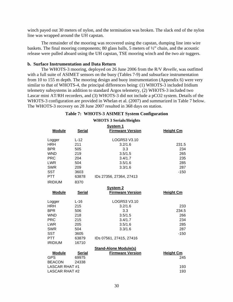
The WHOTS-3 mooring, deployed on 26 June 2006 from the R/V Revelle, was outfitted with a full suite of ASIMET sensors on the buoy (Tables 7-9) and subsurface instrumentation from 10 to 155 m depth. The mooring design and buoy instrumentation (Appendix 6) were very similar to that of WHOTS-4, the principal differences being: (1) WHOTS-3 included Iridium telemetry subsystems in addition to standard Argos telemetry, (2) WHOTS-3 included two Lascar mini AT/RH recorders, and (3) WHOTS-3 did not include a pCO2 system. Details of the WHOTS-3 configuration are provided in Whelan et al. (2007) and summarized in Table 7 below. The WHOTS-3 recovery on 28 June 2007 resulted in 368 days on station.

Table 7: WHOTS-3 ASIMET System Configuration WHOTS 3 Serials/Heights

System 1 Module Serial Firmware Version Height Cm

Logger L-12 LOGR53 V3.10 HRH 211 3.2/1.6 231.5 BPR 505 3.3 234 WND 219 3.5/1.5 265 PRC 204 3.4/1.7 235 LWR 504 3.5/1.6 285 SWR 209 3.3/1.6 287 SST 3603 -150 PTT 63878 IDs 27356, 27364, 27413 IRIDIUM 8370 System 2

Module Serial Firmware Version Height Cm Logger L-16 LOGR53 V3.10 HRH 215 3.2/1.6 233 BPR 506 3.3 234.5 WND 218 3.5/1.5 266 PRC 215 3.4/1.7 234 LWR 205 3.5/1.6 285 SWR 504 3.3/1.6 287 SST 3605 -150 PTT 63879 IDs 07561, 27415, 27416 IRIDIUM 16710 Stand-Alone Module(s)

Module Serial Firmware Version Height Cm GPS 69975 245 BEACON 24338 LASCAR RHAT #1 193 LASCAR RHAT #2 193

31

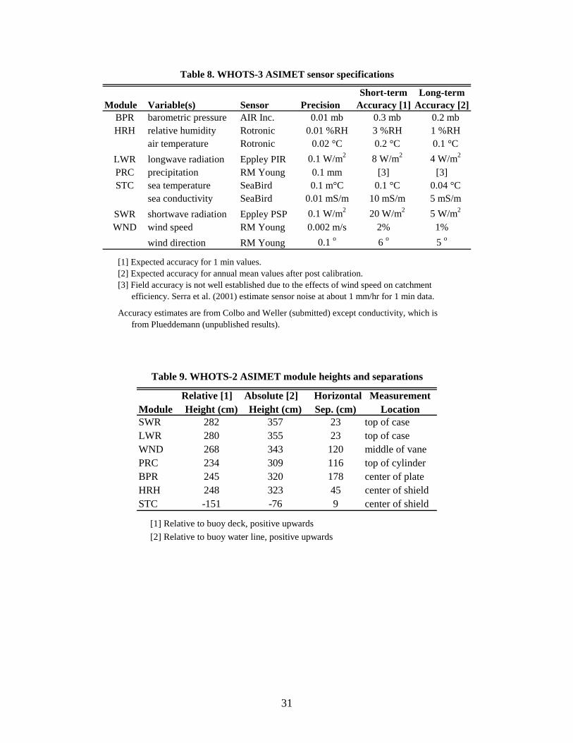
Short-term Long-termModule Variable(s) Sensor Precision Accuracy [1] Accuracy [2]

BPR barometric pressure AIR Inc. 0.01 mb 0.3 mb 0.2 mbHRH relative humidity Rotronic 0.01 %RH 3 %RH 1 %RH

air temperature Rotronic 0.02 °C 0.2 °C 0.1 °CLWR longwave radiation Eppley PIR 0.1 W/m2 8 W/m2 4 W/m2

PRC precipitation RM Young 0.1 mm [3] [3]STC sea temperature SeaBird 0.1 m°C 0.1 °C 0.04 °C

sea conductivity SeaBird 0.01 mS/m 10 mS/m 5 mS/mSWR shortwave radiation Eppley PSP 0.1 W/m2 20 W/m2 5 W/m2

WND wind speed RM Young 0.002 m/s 2% 1%wind direction RM Young 0.1 o 6 o 5 o

[3] Field accuracy is not well established due to the effects of wind speed on catchment efficiency. Serra et al. (2001) estimate sensor noise at about 1 mm/hr for 1 min data.

from Plueddemann (unpublished results).

Table 8. WHOTS-3 ASIMET sensor specifications

[1] Expected accuracy for 1 min values. [2] Expected accuracy for annual mean values after post calibration.

Accuracy estimates are from Colbo and Weller (submitted) except conductivity, which is

Relative [1] Absolute [2] Horizontal MeasurementModule Height (cm) Height (cm) Sep. (cm) LocationSWR 282 357 23 top of caseLWR 280 355 23 top of caseWND 268 343 120 middle of vanePRC 234 309 116 top of cylinderBPR 245 320 178 center of plateHRH 248 323 45 center of shieldSTC -151 -76 9 center of shield

Table 9. WHOTS-2 ASIMET module heights and separations

[1] Relative to buoy deck, positive upwards [2] Relative to buoy water line, positive upwards

32

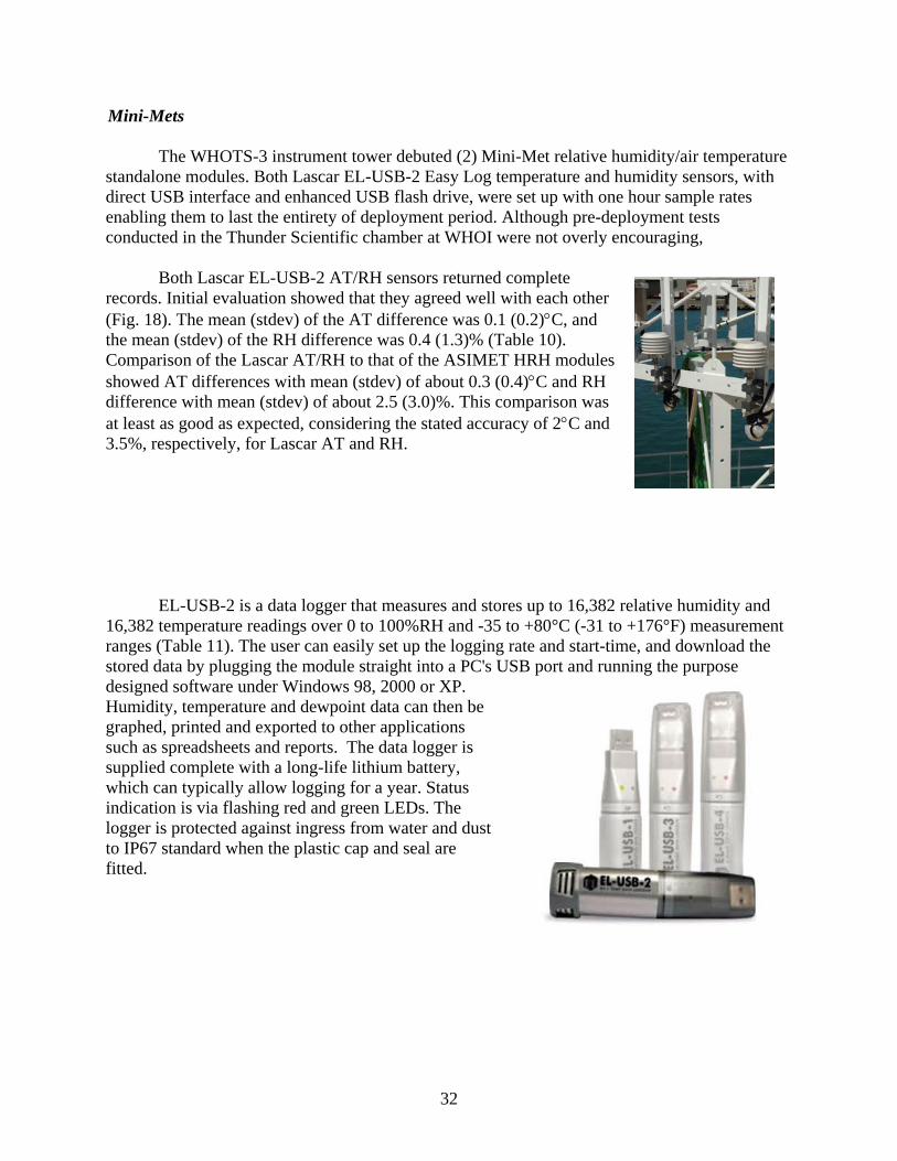
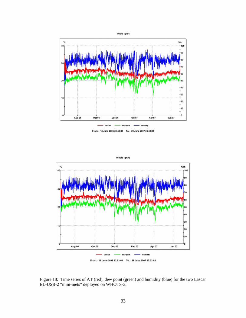
Mini-Mets The WHOTS-3 instrument tower debuted (2) Mini-Met relative humidity/air temperature

standalone modules. Both Lascar EL-USB-2 Easy Log temperature and humidity sensors, with direct USB interface and enhanced USB flash drive, were set up with one hour sample rates enabling them to last the entirety of deployment period. Although pre-deployment tests conducted in the Thunder Scientific chamber at WHOI were not overly encouraging,

Both Lascar EL-USB-2 AT/RH sensors returned complete

records. Initial evaluation showed that they agreed well with each other (Fig. 18). The mean (stdev) of the AT difference was 0.1 (0.2)°C, and the mean (stdev) of the RH difference was 0.4 (1.3)% (Table 10). Comparison of the Lascar AT/RH to that of the ASIMET HRH modules showed AT differences with mean (stdev) of about 0.3 (0.4)°C and RH difference with mean (stdev) of about 2.5 (3.0)%. This comparison was at least as good as expected, considering the stated accuracy of 2°C and 3.5%, respectively, for Lascar AT and RH.

EL-USB-2 is a data logger that measures and stores up to 16,382 relative humidity and

16,382 temperature readings over 0 to 100%RH and -35 to +80°C (-31 to +176°F) measurement ranges (Table 11). The user can easily set up the logging rate and start-time, and download the stored data by plugging the module straight into a PC's USB port and running the purpose designed software under Windows 98, 2000 or XP. Humidity, temperature and dewpoint data can then be graphed, printed and exported to other applications such as spreadsheets and reports. The data logger is supplied complete with a long-life lithium battery, which can typically allow logging for a year. Status indication is via flashing red and green LEDs. The logger is protected against ingress from water and dust to IP67 standard when the plastic cap and seal are fitted.

33

Figure 18: Time series of AT (red), dew point (green) and humidity (blue) for the two Lascar EL-USB-2 “mini-mets” deployed on WHOTS-3.

34

Table 10: Lascar EL-USB-2 performance

Temp RH Dew Standard Deviation 0.236403 1.275932 0.346223Mean -0.12003 0.421885 -0.02717 Variation 0.05588 1.627822 0.119857

On average there was a difference of .12003 between both sensors.

Available sample rates and memory capacities are as follows:

Table 11: Lascar EL-USB-2 sample and memory

Sample Rate Memory Capacity _10 seconds _45 hours _1 minute _11 days _5 minutes _56 days _30 minutes _11 months _1 hour _1.8 years _6 hours _> 2 years* _12 hours _> 2 years*

* Although you can log at this sample rate, the battery will in all likelihood run out before you have filled the EL-USB-2's memory.

FSST

Internally logging Sea-Bird SBE-39 and RBR 1050 temperature sensors were mounted beneath a foam flotation cylinder on the outside face of the buoy hull. Vertical rails allowed the foam to move up and down with the waves, so that the sensor measured the SST within the upper 10-20 cm of the water column. Unfortunately, no data were able to be offloaded from either of the “floating” SST sensors, because serial communication to the instruments could not be established. Thus, it was not clear whether data had been written and might be recoverable later.

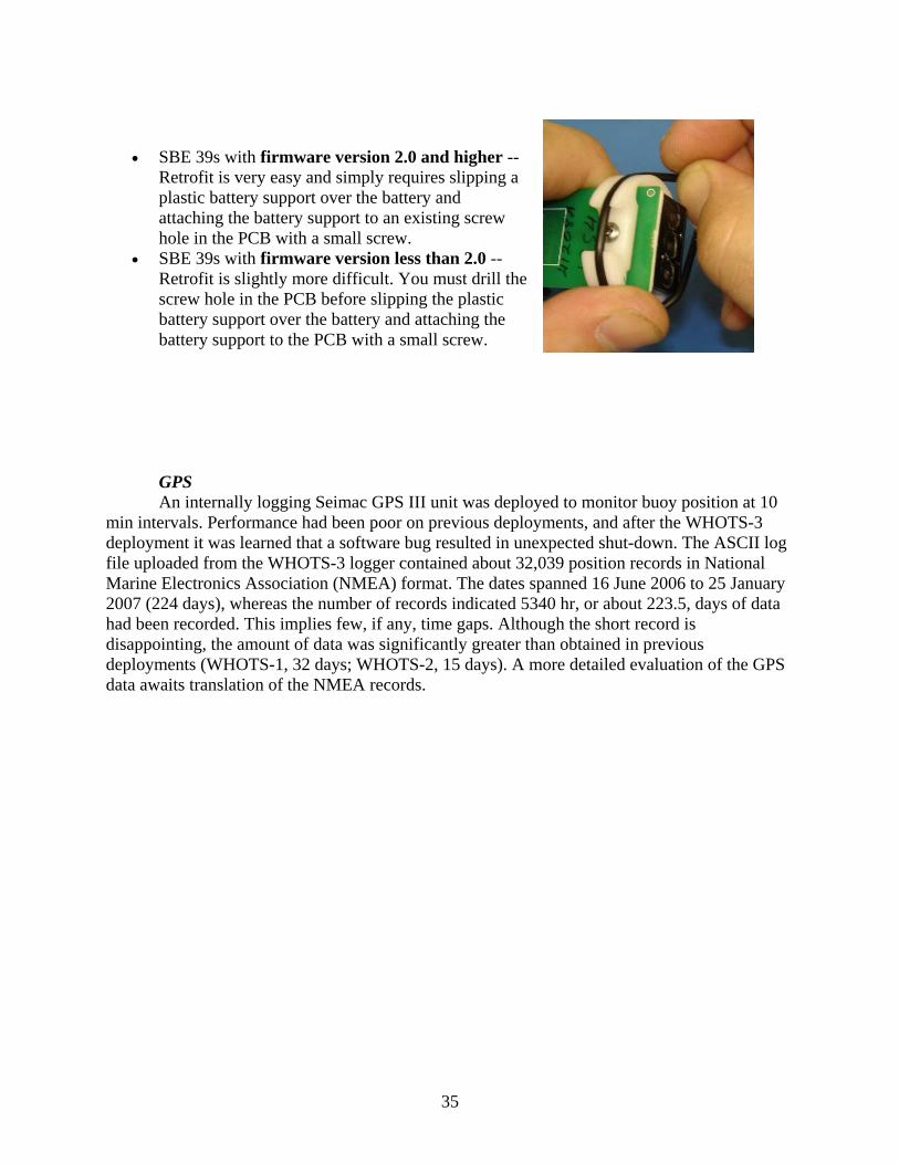
Description of problem: Strong repetitive motions, such as cable strumming or vibrations on a towed net / sled can cause the SBE 39’s internal battery to vibrate. In a few cases of severe vibration, the battery movement cracked the PCB, affecting operation of the instrument and resulting in loss of data. Solution:

Sea-Bird can provide a battery support retrofit kit, PN 50419. The retrofit holds the battery firmly in place, preventing battery movement due to cable strumming or vibrations:

35

• SBE 39s with firmware version 2.0 and higher -- Retrofit is very easy and simply requires slipping a plastic battery support over the battery and attaching the battery support to an existing screw hole in the PCB with a small screw.

• SBE 39s with firmware version less than 2.0 -- Retrofit is slightly more difficult. You must drill the screw hole in the PCB before slipping the plastic battery support over the battery and attaching the battery support to the PCB with a small screw.

GPS An internally logging Seimac GPS III unit was deployed to monitor buoy position at 10

min intervals. Performance had been poor on previous deployments, and after the WHOTS-3 deployment it was learned that a software bug resulted in unexpected shut-down. The ASCII log file uploaded from the WHOTS-3 logger contained about 32,039 position records in National Marine Electronics Association (NMEA) format. The dates spanned 16 June 2006 to 25 January 2007 (224 days), whereas the number of records indicated 5340 hr, or about 223.5, days of data had been recorded. This implies few, if any, time gaps. Although the short record is disappointing, the amount of data was significantly greater than obtained in previous deployments (WHOTS-1, 32 days; WHOTS-2, 15 days). A more detailed evaluation of the GPS data awaits translation of the NMEA records.

36

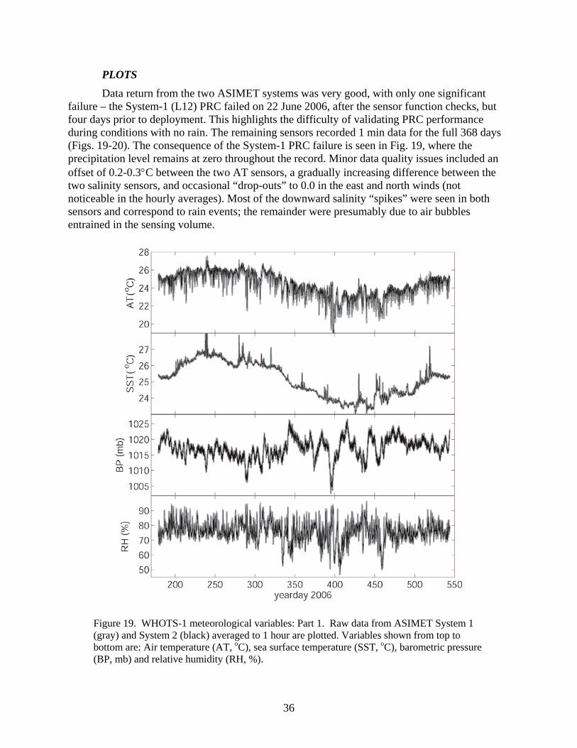
PLOTS Data return from the two ASIMET systems was very good, with only one significant

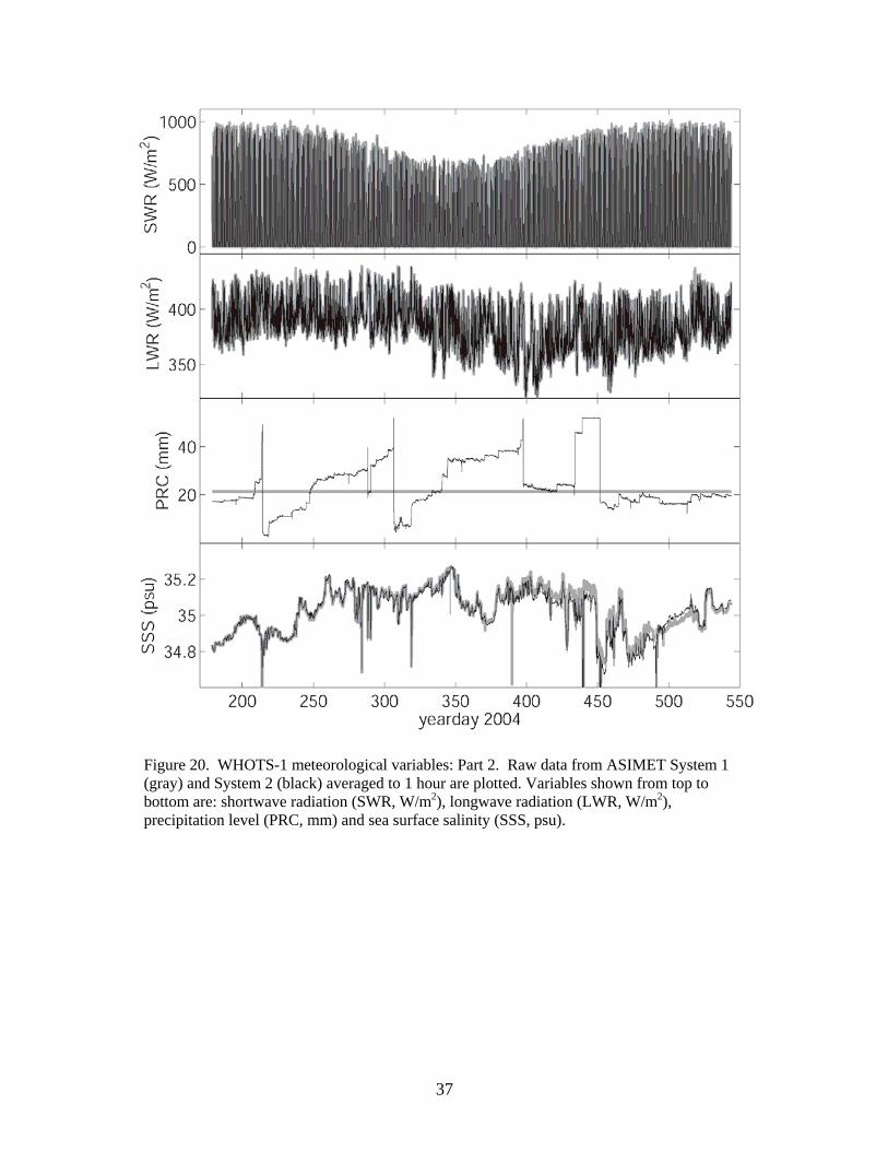
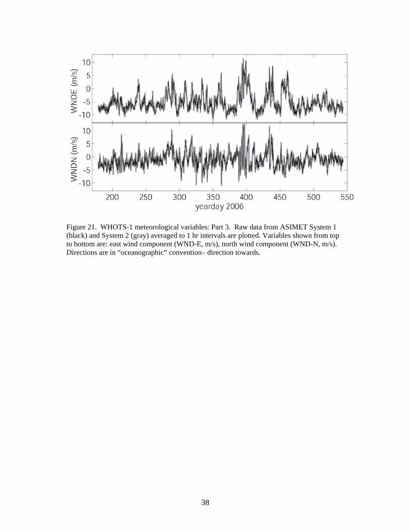
failure – the System-1 (L12) PRC failed on 22 June 2006, after the sensor function checks, but four days prior to deployment. This highlights the difficulty of validating PRC performance during conditions with no rain. The remaining sensors recorded 1 min data for the full 368 days (Figs. 19-20). The consequence of the System-1 PRC failure is seen in Fig. 19, where the precipitation level remains at zero throughout the record. Minor data quality issues included an offset of 0.2-0.3°C between the two AT sensors, a gradually increasing difference between the two salinity sensors, and occasional “drop-outs” to 0.0 in the east and north winds (not noticeable in the hourly averages). Most of the downward salinity “spikes” were seen in both sensors and correspond to rain events; the remainder were presumably due to air bubbles entrained in the sensing volume.

Figure 19. WHOTS-1 meteorological variables: Part 1. Raw data from ASIMET System 1 (gray) and System 2 (black) averaged to 1 hour are plotted. Variables shown from top to bottom are: Air temperature (AT, oC), sea surface temperature (SST, oC), barometric pressure (BP, mb) and relative humidity (RH, %).

37

Figure 20. WHOTS-1 meteorological variables: Part 2. Raw data from ASIMET System 1 (gray) and System 2 (black) averaged to 1 hour are plotted. Variables shown from top to bottom are: shortwave radiation (SWR, W/m2), longwave radiation (LWR, W/m2), precipitation level (PRC, mm) and sea surface salinity (SSS, psu).

38

Figure 21. WHOTS-1 meteorological variables: Part 3. Raw data from ASIMET System 1 (black) and System 2 (gray) averaged to 1 hr intervals are plotted. Variables shown from top to bottom are: east wind component (WND-E, m/s), north wind component (WND-N, m/s). Directions are in “oceanographic” convention– direction towards.

39

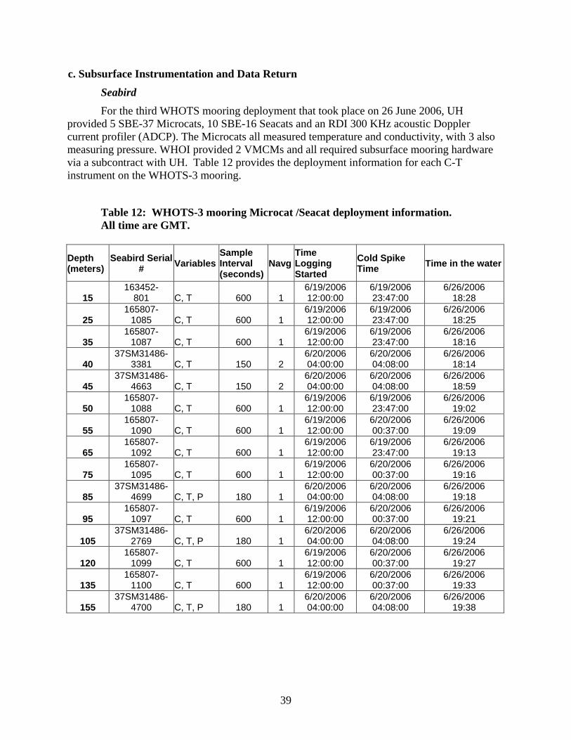
c. Subsurface Instrumentation and Data Return

Seabird For the third WHOTS mooring deployment that took place on 26 June 2006, UH

provided 5 SBE-37 Microcats, 10 SBE-16 Seacats and an RDI 300 KHz acoustic Doppler current profiler (ADCP). The Microcats all measured temperature and conductivity, with 3 also measuring pressure. WHOI provided 2 VMCMs and all required subsurface mooring hardware via a subcontract with UH. Table 12 provides the deployment information for each C-T instrument on the WHOTS-3 mooring.

Table 12: WHOTS-3 mooring Microcat /Seacat deployment information. All time are GMT.

Depth (meters)

Seabird Serial # Variables

Sample Interval (seconds)

NavgTime Logging Started

Cold Spike Time Time in the water

15 163452-

801 C, T 600 1 6/19/2006 12:00:00

6/19/2006 23:47:00

6/26/2006 18:28

25 165807-

1085 C, T 600 1 6/19/2006 12:00:00

6/19/2006 23:47:00

6/26/2006 18:25

35 165807-

1087 C, T 600 1 6/19/2006 12:00:00

6/19/2006 23:47:00

6/26/2006 18:16

40 37SM31486-

3381 C, T 150 2 6/20/2006 04:00:00

6/20/2006 04:08:00

6/26/2006 18:14

45 37SM31486-

4663 C, T 150 2 6/20/2006 04:00:00

6/20/2006 04:08:00

6/26/2006 18:59

50 165807-

1088 C, T 600 1 6/19/2006 12:00:00

6/19/2006 23:47:00

6/26/2006 19:02

55 165807-

1090 C, T 600 1 6/19/2006 12:00:00

6/20/2006 00:37:00

6/26/2006 19:09

65 165807-

1092 C, T 600 1 6/19/2006 12:00:00

6/19/2006 23:47:00

6/26/2006 19:13

75 165807-

1095 C, T 600 1 6/19/2006 12:00:00

6/20/2006 00:37:00

6/26/2006 19:16

85 37SM31486-

4699 C, T, P 180 1 6/20/2006 04:00:00

6/20/2006 04:08:00

6/26/2006 19:18

95 165807-

1097 C, T 600 1 6/19/2006 12:00:00

6/20/2006 00:37:00

6/26/2006 19:21

105 37SM31486-

2769 C, T, P 180 1 6/20/2006 04:00:00

6/20/2006 04:08:00

6/26/2006 19:24

120 165807-

1099 C, T 600 1 6/19/2006 12:00:00

6/20/2006 00:37:00

6/26/2006 19:27

135 165807-

1100 C, T 600 1 6/19/2006 12:00:00

6/20/2006 00:37:00

6/26/2006 19:33

155 37SM31486-

4700 C, T, P 180 1 6/20/2006 04:00:00

6/20/2006 04:08:00

6/26/2006 19:38

40

Table 13. WHOTS-3 mooring Seacat and Microcat recovery information. All times are GMT.

Depth (meters)

Seabird Serial #

Time out of water

Time of Spike

Time Logging Stopped

Samples Logged

Data Quality

File Name raw data

15 163452-

0801 6/28/2007

17:28 06/28/2007

20:21:00 06/28/2007

21:12:00 53192 good whots3_seacat_801.hex

25 165807-

1085 6/28/2007

17:40 06/28/2007

20:21:00 Not Logging 31182 good but

incomplete whots3_seacat_1085.hex

35 165807-

1087 6/28/2007

17:44 06/28/2007

20:21:00 Not Logging 22758 good but

incomplete whots3_seacat_1087.hex

40 37SM31486-

3381 6/28/2007

17:49 06/28/2007

21:00:00 06/29/2007

03:07:00 215402 good whots3_m_3381.asc

45 37SM31486-

4663 6/28/2007

17:50 06/28/2007

21:00:00 06/28/2007

23:26:00 215315 good whots3_m_4663.asc

50 165807-

1088 6/28/2007

17:53 06/28/2007

20:21:00 06/29/2007

00:43:45 53932 good whots3_seacat_1088.hex

55 165807-

1090 6/28/2007

17:55 06/28/2007

20:21:00 06/29/2007

00:57:00 53934 good whots3_seacat_1090.hex

65 165807-

1092 6/28/2007

17:59 06/28/2007

20:21:00 06/29/2007

01:09:00 53985 good whots3_seacat_1092.hex

75 165807-

1095 6/28/2007

18:02 06/28/2007

20:21:00 06/29/2007

01:28:00 53937 T problem 2 months whots3_seacat_1095.hex

85 37SM31486-

4699 6/28/2007

18:05 06/28/2007

21:00:00 06/29/2007

03:06:00 179501 good whots3_p_4699.asc

95 165807-

1097 6/28/2007

18:07 06/28/2007

20:21:00 06/29/2007

01:39:00 53938 good whots3_seacat_1097.hex

105 37SM31486-

2769 6/28/2007

18:10 06/28/2007

21:00:00 06/28/2007

23:29:00 179430 good whots3_p_2769.asc

120 165807-

1099 6/28/2007

18:13 06/28/2007

21:00:00 06/29/2007

01:58:00 53940 good whots3_seacat_1099.hex

135 165807-

1100 6/28/2007

18:21 06/28/2007

21:00:00 06/29/2007

02:07:00 53906 good whots3_seacat_1100.hex

155 37SM31486-

4700 6/28/2007

18:25 06/28/2007

21:00:00 06/28/2007

23:24:00 17428 P sensor

failed whots3_p_4700.asc

All instruments on the mooring were successfully recovered. Most of the instruments had some degree of biofouling, with the heaviest fouling near the surface. Fouling extended down to the ADCP at 125 m. However, the C-T instruments at 65 m, 95 m, and 120 m had minimal fouling. The reason for the relatively unfouled instruments at the shallower depths is not known.

Table 13 gives post-deployment information for the C-T instruments. Table 14 gives post-deployment information for the VMCMs. Table 15 gives post-deployment information for the ADCP.

All but two instruments returned full data records. The Seacats at 25 m and 35 m were not operating upon recovery, but returned partial data records, approximately 50% and 30% respectively. The pressure sensor on the 155 m Microcat started to drift soon after deployment, and then failed. Temperature and conductivity on this instrument appear to be unaffected. The temperature record on the 75 m Seacat has two month-long periods of questionable data quality, one around the time of deployment, and the other during February 2007.

With the exceptions noted above, the data recovered from the Microcats and Seacats appear to be of high quality, although post-deployment calibrations are required. Figures D1-D15

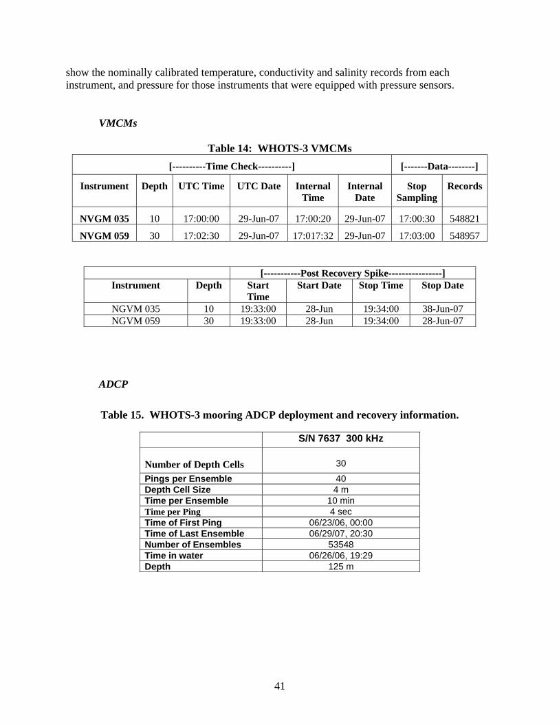
41

show the nominally calibrated temperature, conductivity and salinity records from each instrument, and pressure for those instruments that were equipped with pressure sensors.

VMCMs

Table 14: WHOTS-3 VMCMs [----------Time Check----------] [-------Data--------]

Instrument Depth UTC Time UTC Date Internal Time

Internal Date

Stop Sampling

Records

NVGM 035 10 17:00:00 29-Jun-07 17:00:20 29-Jun-07 17:00:30 548821

NVGM 059 30 17:02:30 29-Jun-07 17:017:32 29-Jun-07 17:03:00 548957

[-----------Post Recovery Spike----------------] Instrument Depth Start

Time Start Date Stop Time Stop Date

NGVM 035 10 19:33:00 28-Jun 19:34:00 38-Jun-07 NGVM 059 30 19:33:00 28-Jun 19:34:00 28-Jun-07

ADCP

Table 15. WHOTS-3 mooring ADCP deployment and recovery information.

S/N 7637 300 kHz

Number of Depth Cells

30

Pings per Ensemble 40 Depth Cell Size 4 m Time per Ensemble 10 min Time per Ping 4 sec Time of First Ping 06/23/06, 00:00 Time of Last Ensemble 06/29/07, 20:30 Number of Ensembles 53548 Time in water 06/26/06, 19:29 Depth 125 m

42

The fouling on the ADCP transducer head (Fig. 22) was greater than during the previous two WHOTS ADCP deployments at 125 m. The data will be closely inspected for any evidence of degradation due to this fouling. The transducer faces should be treated with an appropriate antifouling compound in the future.

Figure 22. WHOTS-3 ADCP deployed at 125 m after recovery.

The data from the upward-looking ADCP at 125 m appears to be of high quality. The heading, pitch and roll information from the ADCP (Fig. 23) provide useful information about the overall behavior of the mooring during its deployment. An example is that the buoy apparently was twisted 2-1/2 turns between mid-October 2006 and early April 2007, and then untwisted one turn during the following two weeks. Pitch and roll are generally less than 5 degrees from the vertical, but there are some periods with deviations from the vertical of as much as 10 degrees.

Figure 24 shows the variations of the horizontal and vertical components of velocity in depth and time. The acoustic returns from the upper 40 m of the water column are intermittent, due to very low levels of scattering material near the surface. Diurnal migration of plankton often allowed good data returns to near the surface at night, however. The high spurious speeds due to sideband reflections near the surface are apparent.

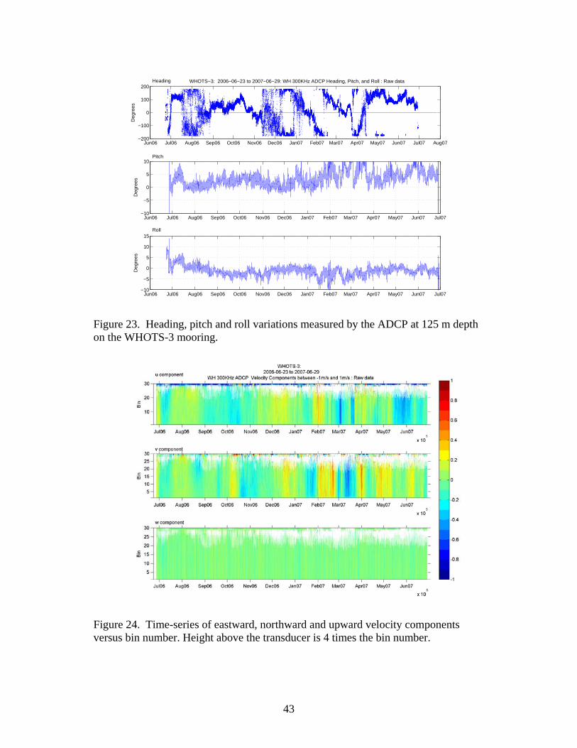
43

Jun06 Jul06 Aug06 Sep06 Oct06 Nov06 Dec06 Jan07 Feb07 Mar07 Apr07 May07 Jun07 Jul07 Aug07−200

−100

0

100

200

Deg

rees

WHOTS−3: 2006−06−23 to 2007−06−29: WH 300KHz ADCP Heading, Pitch, and Roll : Raw data

Jun06 Jul06 Aug06 Sep06 Oct06 Nov06 Dec06 Jan07 Feb07 Mar07 Apr07 May07 Jun07 Jul07−10

−5

0

5

10

Deg

rees

Jun06 Jul06 Aug06 Sep06 Oct06 Nov06 Dec06 Jan07 Feb07 Mar07 Apr07 May07 Jun07 Jul07−10

−5

0

5

10

15

Deg

rees

Heading

Pitch

Roll

Figure 23. Heading, pitch and roll variations measured by the ADCP at 125 m depth on the WHOTS-3 mooring.

Figure 24. Time-series of eastward, northward and upward velocity components versus bin number. Height above the transducer is 4 times the bin number.

44

Kilo Moana has an Uncontaminated Scientific Sea Water (USSW) system

The Kilo Moana has an Uncontaminated Scientific Sea Water (USSW) system that includes an internal Seabird Seacat thermosalinograph model SBE-21, with an SBE-38 external temperature sensor installed in the bow thruster chamber close to the seawater intake. The intake is located on the starboard hull, 20’8” from the bow, at a mean depth of 8 m. Sensor information for the TSG system during WHOTS-4 is as follows:

Temperature: SBE-38 Sensor SN0150 was used to measure temperature near the seawater intake, and was last calibrated on January 11, 2007, and installed on Mar 27, 2007. The SBE-21 thermosalinograph used temperature sensor SN3167, which was last calibrated on December 20, 2006, and installed on May 3, 2007.

Conductivity: The SBE-21 thermosalinograph used conductivity sensor SN3167, which was most recently calibrated on December 20, 2006, and installed on May 03, 2007.

Water samples were drawn from the shipboard Seabird thermosalinograph system roughly every 8 hours during the cruise for post-calibration of that dataset. Shipboard ADCPs

The R/V Kilo Moana is equipped with an RDI 300 kHz Workhorse Mariner ADCP and an RDI OS38 ADCP. The University of Hawaii ADCP processing system is installed, producing real-time profiles and other products. In addition to providing an intercomparison with the upward-looking ADCP on the WHOTS moorings, the shipboard ADCP systems revealed interesting regional current features.

During the WHOTS-4 cruise, we observed the northwestward flow of the North Hawaiian Ridge Current during our transit from Oahu to Station ALOHA (Fig. 13), which was north of the strong flow. The NCOM analysis of 6/27/07 (Fig. 25) was consistent with the ADCP observations. The 38 kHz ADCP revealed an eastward flow of about 20 cm/s centered near 800 m, which is the core depth of the Antarctic Intermediate Water. The thickness of this feature was about 300 m.

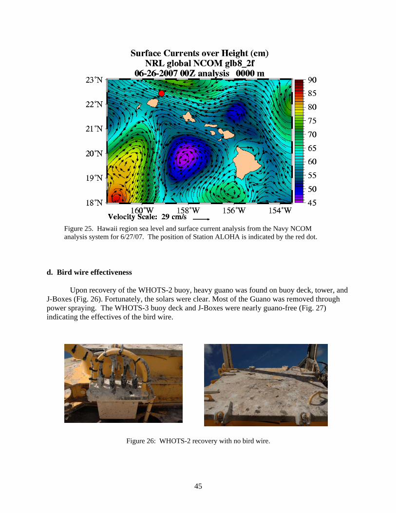
45

Figure 25. Hawaii region sea level and surface current analysis from the Navy NCOM analysis system for 6/27/07. The position of Station ALOHA is indicated by the red dot.

d. Bird wire effectiveness

Upon recovery of the WHOTS-2 buoy, heavy guano was found on buoy deck, tower, and

J-Boxes (Fig. 26). Fortunately, the solars were clear. Most of the Guano was removed through power spraying. The WHOTS-3 buoy deck and J-Boxes were nearly guano-free (Fig. 27) indicating the effectives of the bird wire.

Figure 26: WHOTS-2 recovery with no bird wire.

46

Figure 27: WHOTS-3 recovery with bird wire.

e. Biofouling

This details the antifouling treatment on WHOTS 3 buoy and instrumentation. Waters at

the WHOTS site are not high fouling as compared to an estuarine environment, but there is enough activity to warrant use of antifouling measures. Gooseneck barnacles, the primary concern for increasing weight, drag and likelihood of instrument failures, are prolific down to 30 meters. For this reason, it is critical to protect instrumentation, especially devices with moving parts (VMCM). Because organotin-based antifouling coatings are no longer available and their use in the United States banned, viable alternatives are needed. Alex Walsh of E-Paint has been assisting WHOI with research on antifouling coatings for several years. This research effort evaluates different E Paint coatings for use on oceanographic surface buoys, sensors and the like. Antifouling coatings applied to the WHOTS-2 Buoy and instrumentation are detailed below:

Coat Product Description

1. 2 US Quarts Haze Gray - EP-PRIME 1000 / High Build Epoxy Primer 2. 2 US Quarts Gray – SUNWAVE+ (2.5% Zinc Omadine®) 3. 2 US Quarts White – SUNWAVE+ (2.5% Zinc Omadine®) 4. 2 US Quarts White – SUNWAVE+ (2.5% Zinc Omadine®) 5. 4 US Quarts White – SUNWAVE+ (4.7% Zinc Omadine®)

Coat Product Description

1. 1 US Quart Gray - EP-PRIME 2000 / Epoxy Barrier 2. 1 US Quart White - EP 2000 3. 1 US Quart White- EP 2000 4. 1 US Quart White- EP 2000

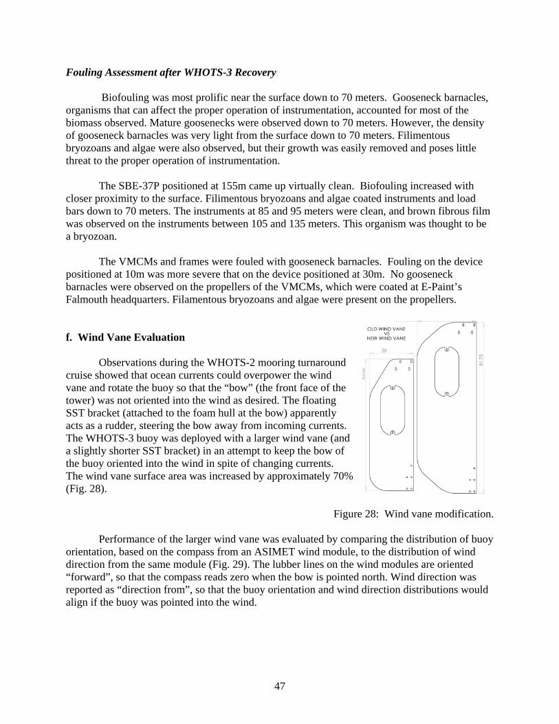
47

Fouling Assessment after WHOTS-3 Recovery

Biofouling was most prolific near the surface down to 70 meters. Gooseneck barnacles, organisms that can affect the proper operation of instrumentation, accounted for most of the biomass observed. Mature goosenecks were observed down to 70 meters. However, the density of gooseneck barnacles was very light from the surface down to 70 meters. Filimentous bryozoans and algae were also observed, but their growth was easily removed and poses little threat to the proper operation of instrumentation.

The SBE-37P positioned at 155m came up virtually clean. Biofouling increased with

closer proximity to the surface. Filimentous bryozoans and algae coated instruments and load bars down to 70 meters. The instruments at 85 and 95 meters were clean, and brown fibrous film was observed on the instruments between 105 and 135 meters. This organism was thought to be a bryozoan.

The VMCMs and frames were fouled with gooseneck barnacles. Fouling on the device

positioned at 10m was more severe that on the device positioned at 30m. No gooseneck barnacles were observed on the propellers of the VMCMs, which were coated at E-Paint’s Falmouth headquarters. Filamentous bryozoans and algae were present on the propellers.

f. Wind Vane Evaluation

Observations during the WHOTS-2 mooring turnaround cruise showed that ocean currents could overpower the wind vane and rotate the buoy so that the “bow” (the front face of the tower) was not oriented into the wind as desired. The floating SST bracket (attached to the foam hull at the bow) apparently acts as a rudder, steering the bow away from incoming currents. The WHOTS-3 buoy was deployed with a larger wind vane (and a slightly shorter SST bracket) in an attempt to keep the bow of the buoy oriented into the wind in spite of changing currents. The wind vane surface area was increased by approximately 70% (Fig. 28).

Figure 28: Wind vane modification.

Performance of the larger wind vane was evaluated by comparing the distribution of buoy orientation, based on the compass from an ASIMET wind module, to the distribution of wind direction from the same module (Fig. 29). The lubber lines on the wind modules are oriented “forward”, so that the compass reads zero when the bow is pointed north. Wind direction was reported as “direction from”, so that the buoy orientation and wind direction distributions would align if the buoy was pointed into the wind.

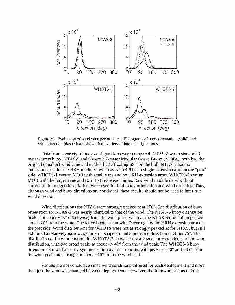
48

Figure 29. Evaluation of wind vane performance. Histograms of buoy orientation (solid) and wind direction (dashed) are shown for a variety of buoy configurations.

Data from a variety of buoy configurations were compared. NTAS-2 was a standard 3-

meter discus buoy. NTAS-5 and 6 were 2.7-meter Modular Ocean Buoys (MOBs), both had the original (smaller) wind vane and neither had a floating SST on the hull. NTAS-5 had no extension arms for the HRH modules, whereas NTAS-6 had a single extension arm on the “port” side. WHOTS-1 was an MOB with small vane and no HRH extension arms. WHOTS-3 was an MOB with the larger vane and two HRH extension arms. Raw wind module data, without correction for magnetic variation, were used for both buoy orientation and wind direction. Thus, although wind and buoy directions are consistent, these results should not be used to infer true wind direction.

Wind distributions for NTAS were strongly peaked near 100°. The distribution of buoy

orientation for NTAS-2 was nearly identical to that of the wind. The NTAS-5 buoy orientation peaked at about +25° (clockwise) from the wind peak, whereas the NTAS-6 orientation peaked about -20° from the wind. The latter is consistent with “steering” by the HRH extension arm on the port side. Wind distributions for WHOTS were not as strongly peaked as for NTAS, but still exhibited a relatively narrow, symmetric shape around a preferred direction of about 75°. The distribution of buoy orientation for WHOTS-2 showed only a vague correspondence to the wind distribution, with two broad peaks at about +/- 40° from the wind peak. The WHOTS-3 buoy orientation showed a nearly symmetric bimodal distribution, with peaks at -20° and +35° from the wind peak and a trough at about +10° from the wind peak.

Results are not conclusive since wind conditions differed for each deployment and more

than just the vane was changed between deployments. However, the following seems to be a

49

reasonable description. First, note that both the 3-meter discus and MOB buoy hulls are symmetric. The 3-meter discus tower is a regular triangle, whereas the MOB tower is an irregular pentagon above a square base. The longest leg of the pentagon faces into the wind. The 3-meter discus buoy, with vane area (~2000 sq in) similar to the larger MOB vane and no floating SST bracket, orients consistently with bow to the wind. The MOB has preferred orientations of roughly +/- 25° from the wind. With no floating SST bracket, one or the other of these orientations is favored throughout the deployment (presumably due to asymmetric placement of sensors on the buoy tower). With floating SST bracket and small vane (~1280 sq in), currents have a significant influence on MOB orientation. The buoy directions are broadly distributed around the wind direction, and orientations up to +/- 60° from the wind are not uncommon. There is only a hint of the preferred orientations, consistent with the idea that currents acting on the SST bracket often overwhelm the wind vane. With the larger vane (~2214 sq in), the MOB with SST bracket tends to “oscillate” between the two preferred orientations, presumably due to currents intermittently pushing the buoy out of one preferred orientation and into the other. The result is a bimodal buoy orientation distribution with peaks at about +/- 30° from the wind direction.

50

6. Meteorological Intercomparisons a. Overview

In order to assess the performance of the buoy meteorological systems, two periods of about 24 h were dedicated to buoy vs. ship intercomparisons. The first inter-comparison period followed deployment of the WHOTS-4 mooring, and the second was prior to recovery of the WHOTS-3 mooring. Hourly ASIMET data were obtained by intercepting the Argos PTT transmissions from the buoy with an Alpha-Omega satellite uplink receiver and a whip antenna mounted on the forward deck rail. Consistent receptions from both PTTs were obtained with the ship standing-off at a distance of about 0.15 nm from the buoy. CTD casts to 200 m were performed during the intercomparison period while holding station near the buoy (see Appendix C). However, the Kilo Moana departed the area twice during each period for sewage and trash disposal. Although the quality of the comparison suffered during these periods, no buoy data were lost since 6 h of buffered data are transmitted by the ASIMET logger PTTs each hour.

As described in Sec. 2d, the shipboard meteorological system used for the intercmparison was an AutoIMET system installed on the Kilo Moana science mast by the UOP group. This system provided barometric pressure (BP), air temperature (AT), relative humidity (RH), shortwave radiation (SWR), longwave radiation (LWR), precipitation (PRC), and wind speed (WSPD), and direction (WDIR) relative to the ship. GPS position data were recorded, but the wind data were not corrected in real-time. The uncorrected AutoIMET wind speed was used here with the assumption that the ship was stationary; uncorrected wind direction was not used. The AutoIMET data, collected at 2 min intervals, were averaged to 1 h for comparison with the buoy systems.

The AutoIMET AT, RH, PRC, SWR and LWR sensors were at approximately 20 m above the waterline, but were not corrected for height. AutoIMET BP (21 m) was corrected to 3 m height to correspond to the buoy. AutoIMET WSPD (22 m) and buoy WSPD (3 m) were adjusted to 10 m using a neutral drag coefficient.

Since the AutoIMET system did not include sensors for sea surface temperature (SST) and sea surface salinity (SSS), the Kilo Moana shipboard systems were used. There were two sources of SST data on the Kilo Moana. Both systems took in water from the bow intake, located at a depth of about 7.5 m. The “remote” probe was physically located at the intake, whereas the thermosalinograph (TSG) measured seawater that had been pumped from the intake to the Met Lab. The experience of HOT investigators comparing Kilo Moana SSTs to CTDs indicated that the remote SST was preferable to the TSG, but read about 0.2°C high relative to the actual water temperature. A correction of -0.2°C was applied for comparison with the buoy. SSS data for comparison with the buoys came directly from the TSG. Both SST and SSS data, available from the shipboard computer system at 10 sec intervals, were averaged to 1 h. b. WHOTS-3 vs. Kilo Moana

The WHOTS-3 intercomparison period started at 1100 h UTC on 27 June (year day 178.46) when the first Argos transmissions were received upon approaching the WHOTS-3 buoy. Operations continued until 1500 h UTC on 28 June (year day 179.63), just before the release was fired. The total duration was 28 h. The Kilo Moana departed the site twice, near

51

yearday 179.1 and 179.4, for sewage and trash disposal. The results of the comparison are shown in Figures 30-34. The buoy systems are identified in the plots by their logger numbers (L12=WHOTS-3 System 1, L16=WHOTS-3 System 2). The buoy sensor pairs showed good agreement (differences between like sensors were within the expected short-term accuracy; Table x) for all variables except AT, SSS and SWR. Examination of the buoy data in conjunction with the shipboard meteorology provided further understanding of these discrepancies, and resulted in other useful observations about system performance, as described below.

The WHOTS-3 buoy AT pair disagreed by about 0.25°C, with L16 reading higher than

L12. Buoy AT values were consistently higher than the shipboard AT by 0.2°C (L12) to 0.45°C (L16). Buoy AT offsets of about +0.2°C have been seen in previous comparisons, and attributed to vertical gradients between buoy and ship sensors. Thus, it can be inferred that L16 is reading high while L12 is approximately correct. Buoy and shipboard RH generally agreed to within the Argos resolution of 1%. The relatively large discrepancies between buoy and ship for both AT and RH near yearday=179.4 are associated with the Kilo Moana temporarily departing station. The buoy BP pair showed L12 > L16 by about 0.5 mb (difficult to determine precisely given the Argos resolution of 1 mb). The adjusted shipboard BP agreed better with L16 than with L12, suggesting that L16 provided the more accurate BP value. None of the three PRC sensors indicated rain during the intercomparison period. Buoy (1 m depth) and shipboard (7.5 m) SST typically agreed to within 0.1°C. The WHOTS-3 SSS pair showed somewhat erratic behavior, with differences varying from < 0.01 psu to nearly 0.08 psu (for a temperature of 25.3°C, conductivity accuracy of 0.01 S/m translates to a salinity accuracy of about 0.07 psu). The shipboard SSS was much more stable, and about 0.3 psu higher than the buoy sensors on average. The reason for the differences between buoy and ship SSS behavior is not clear. The buoy SWR pair agreed to within 50 W/m2 during most of the day, but showed differences of up to 100 W/m2 (12%) near midday. Relative timing differences between the two loggers may contribute to these discrepancies. The shipboard SWR was typically within 50 W/m2 of the buoy values, tending to be lower before midday and higher after midday. This indicates clock drift in the buoy loggers. The buoy LWR pair agreed to within 5 W/m2 throughout the intercomparison period, while the shipboard LWR was about 5 W/m2 higher than the average of the buoy systems. Buoy wind speeds agreed to 0.2 m/s. Shipboard winds were about 0.5 m/s higher than the buoy, with larger discrepancies near yearday=179.1 and 179.4 when the Kilo Moana departed station. This was considered good agreement given that shipboard winds were uncorrected for ship motion. Buoy wind directions agreed to within 2°–3°.

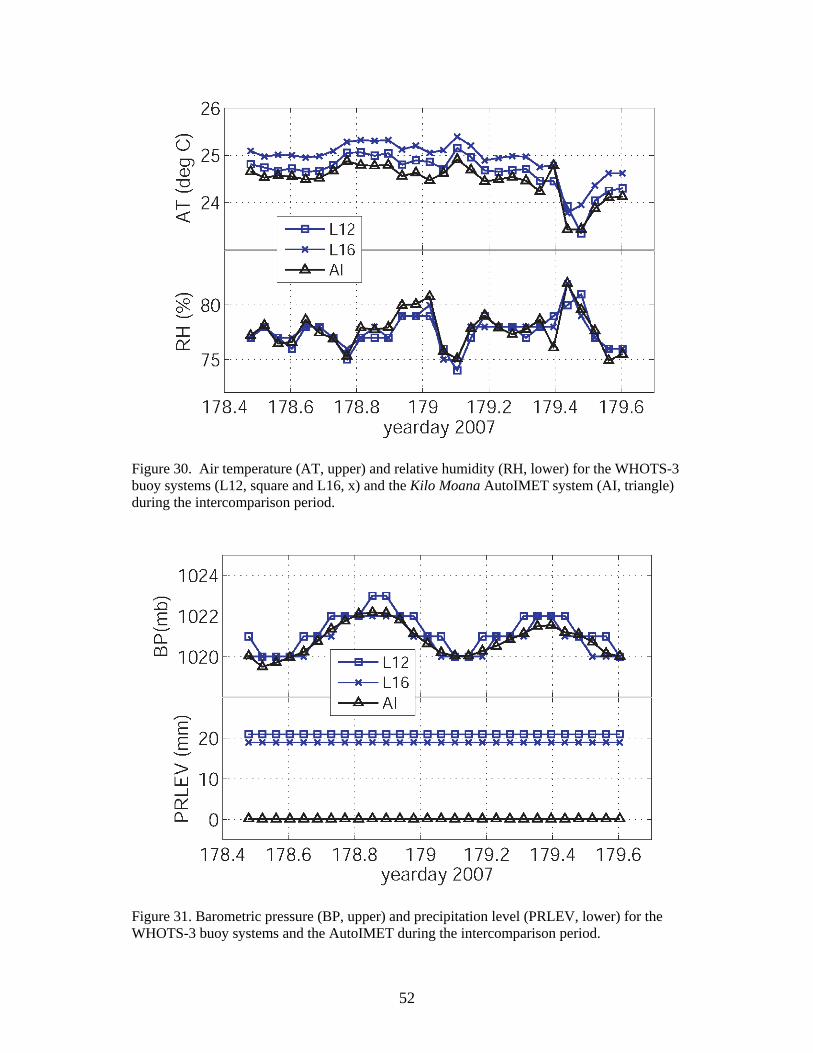
52

Figure 30. Air temperature (AT, upper) and relative humidity (RH, lower) for the WHOTS-3 buoy systems (L12, square and L16, x) and the Kilo Moana AutoIMET system (AI, triangle) during the intercomparison period.

Figure 31. Barometric pressure (BP, upper) and precipitation level (PRLEV, lower) for the WHOTS-3 buoy systems and the AutoIMET during the intercomparison period.

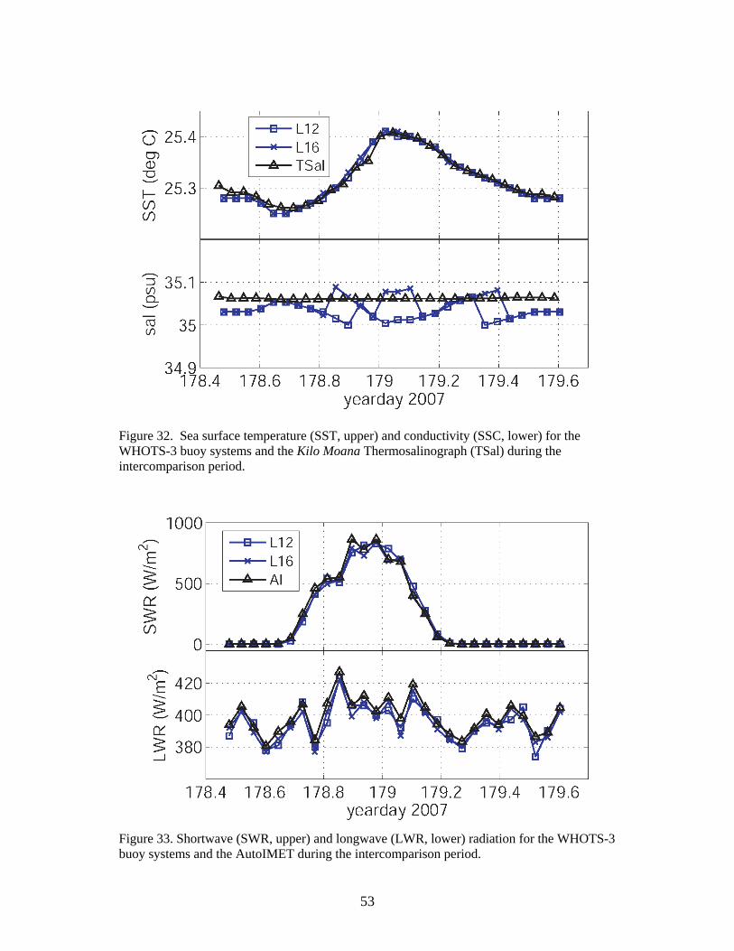
53

Figure 32. Sea surface temperature (SST, upper) and conductivity (SSC, lower) for the WHOTS-3 buoy systems and the Kilo Moana Thermosalinograph (TSal) during the intercomparison period.

Figure 33. Shortwave (SWR, upper) and longwave (LWR, lower) radiation for the WHOTS-3 buoy systems and the AutoIMET during the intercomparison period.

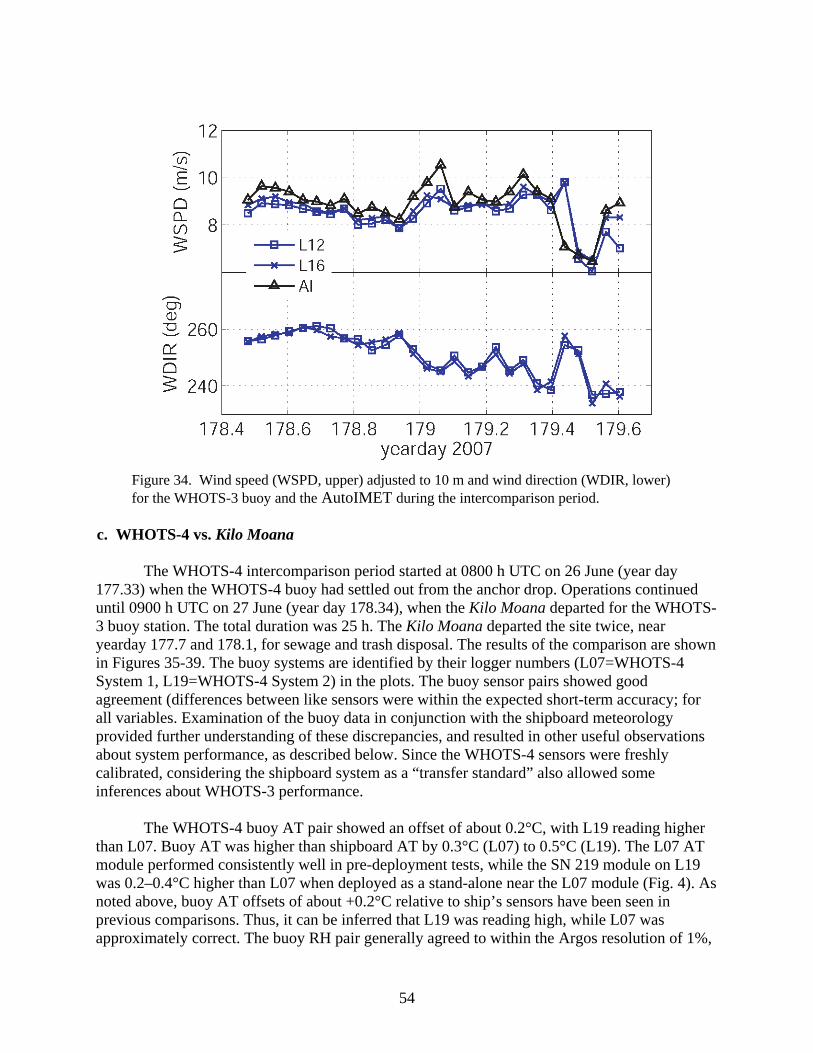
54

Figure 34. Wind speed (WSPD, upper) adjusted to 10 m and wind direction (WDIR, lower) for the WHOTS-3 buoy and the AutoIMET during the intercomparison period.

c. WHOTS-4 vs. Kilo Moana

The WHOTS-4 intercomparison period started at 0800 h UTC on 26 June (year day 177.33) when the WHOTS-4 buoy had settled out from the anchor drop. Operations continued until 0900 h UTC on 27 June (year day 178.34), when the Kilo Moana departed for the WHOTS-3 buoy station. The total duration was 25 h. The Kilo Moana departed the site twice, near yearday 177.7 and 178.1, for sewage and trash disposal. The results of the comparison are shown in Figures 35-39. The buoy systems are identified by their logger numbers (L07=WHOTS-4 System 1, L19=WHOTS-4 System 2) in the plots. The buoy sensor pairs showed good agreement (differences between like sensors were within the expected short-term accuracy; for all variables. Examination of the buoy data in conjunction with the shipboard meteorology provided further understanding of these discrepancies, and resulted in other useful observations about system performance, as described below. Since the WHOTS-4 sensors were freshly calibrated, considering the shipboard system as a “transfer standard” also allowed some inferences about WHOTS-3 performance.

The WHOTS-4 buoy AT pair showed an offset of about 0.2°C, with L19 reading higher

than L07. Buoy AT was higher than shipboard AT by 0.3°C (L07) to 0.5°C (L19). The L07 AT module performed consistently well in pre-deployment tests, while the SN 219 module on L19 was 0.2–0.4°C higher than L07 when deployed as a stand-alone near the L07 module (Fig. 4). As noted above, buoy AT offsets of about +0.2°C relative to ship’s sensors have been seen in previous comparisons. Thus, it can be inferred that L19 was reading high, while L07 was approximately correct. The buoy RH pair generally agreed to within the Argos resolution of 1%,

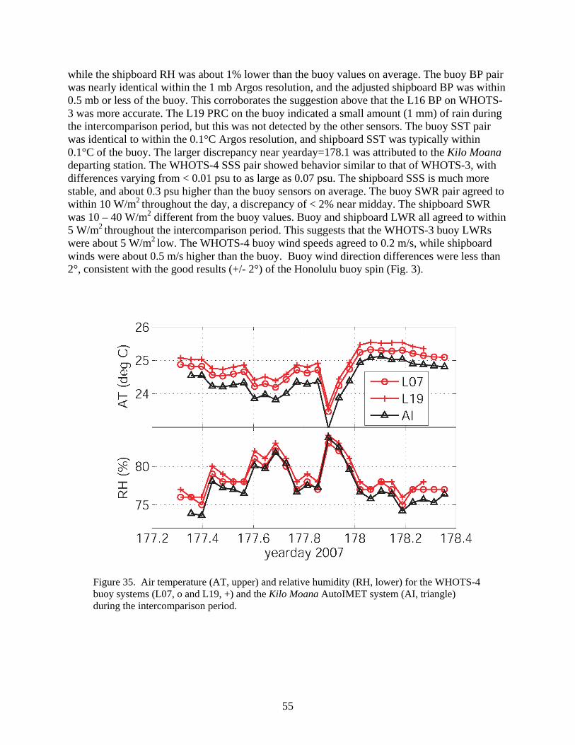
55

while the shipboard RH was about 1% lower than the buoy values on average. The buoy BP pair was nearly identical within the 1 mb Argos resolution, and the adjusted shipboard BP was within 0.5 mb or less of the buoy. This corroborates the suggestion above that the L16 BP on WHOTS-3 was more accurate. The L19 PRC on the buoy indicated a small amount (1 mm) of rain during the intercomparison period, but this was not detected by the other sensors. The buoy SST pair was identical to within the 0.1°C Argos resolution, and shipboard SST was typically within 0.1°C of the buoy. The larger discrepancy near yearday=178.1 was attributed to the Kilo Moana departing station. The WHOTS-4 SSS pair showed behavior similar to that of WHOTS-3, with differences varying from < 0.01 psu to as large as 0.07 psu. The shipboard SSS is much more stable, and about 0.3 psu higher than the buoy sensors on average. The buoy SWR pair agreed to within 10 W/m2 throughout the day, a discrepancy of < 2% near midday. The shipboard SWR was 10 – 40 W/m2 different from the buoy values. Buoy and shipboard LWR all agreed to within 5 W/m2 throughout the intercomparison period. This suggests that the WHOTS-3 buoy LWRs were about 5 W/m2 low. The WHOTS-4 buoy wind speeds agreed to 0.2 m/s, while shipboard winds were about 0.5 m/s higher than the buoy. Buoy wind direction differences were less than 2°, consistent with the good results (+/- 2°) of the Honolulu buoy spin (Fig. 3).

Figure 35. Air temperature (AT, upper) and relative humidity (RH, lower) for the WHOTS-4 buoy systems (L07, o and L19, +) and the Kilo Moana AutoIMET system (AI, triangle) during the intercomparison period.

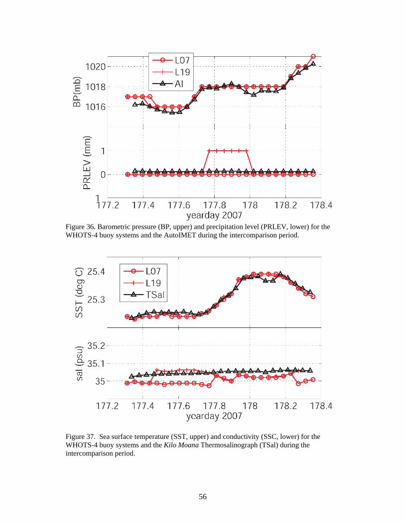
56

Figure 36. Barometric pressure (BP, upper) and precipitation level (PRLEV, lower) for the WHOTS-4 buoy systems and the AutoIMET during the intercomparison period.

Figure 37. Sea surface temperature (SST, upper) and conductivity (SSC, lower) for the WHOTS-4 buoy systems and the Kilo Moana Thermosalinograph (TSal) during the intercomparison period.

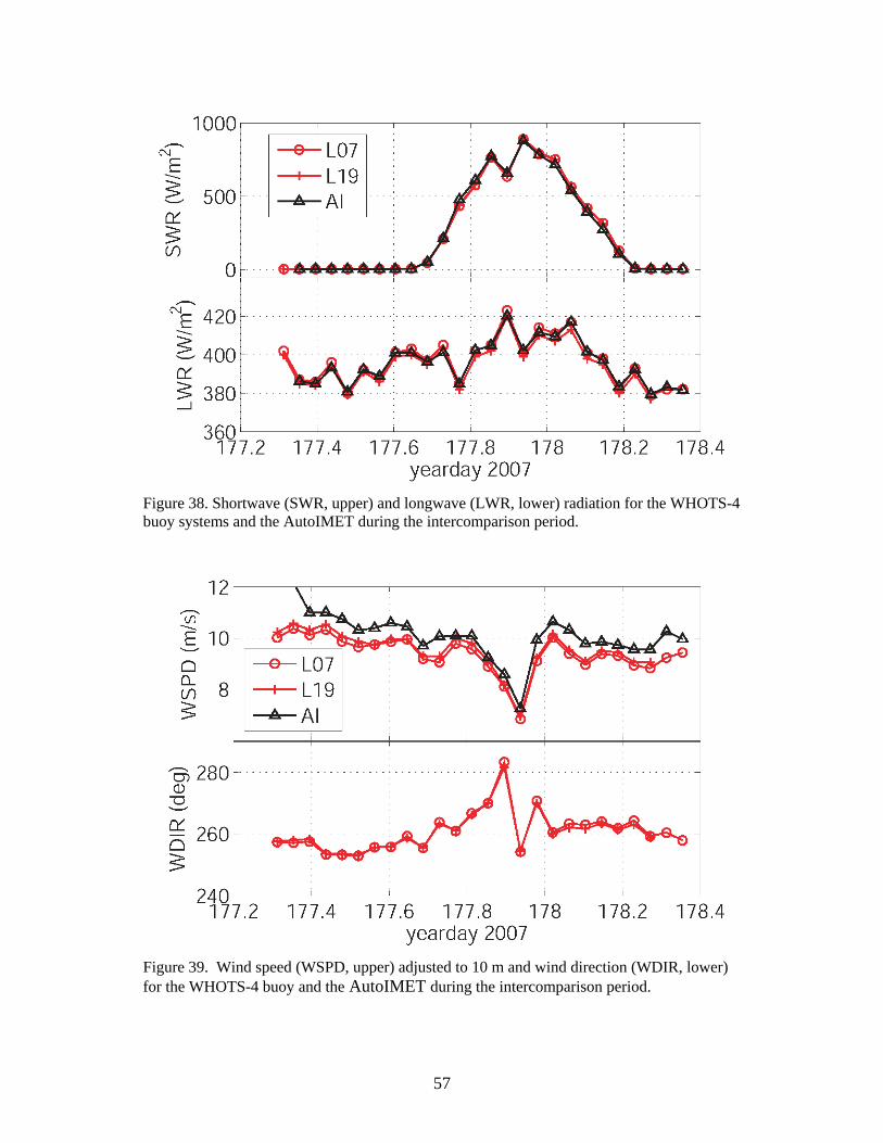
57

Figure 38. Shortwave (SWR, upper) and longwave (LWR, lower) radiation for the WHOTS-4 buoy systems and the AutoIMET during the intercomparison period.

Figure 39. Wind speed (WSPD, upper) adjusted to 10 m and wind direction (WDIR, lower) for the WHOTS-4 buoy and the AutoIMET during the intercomparison period.

58

7. CTD Operations

The University of Hawaii provided CTD and water sampling equipment. A series of CTD casts were made to obtain profiles for comparison with subsurface instruments on the WHOTS-3 mooring before recovery, and with those on the WHOTS-4 mooring after deployment. The comparison series consisted of casts to at least 200 m every two hours for twelve hours (roughly one semidiurnal tidal cycle). In addition, 1000 m CTD profiles were made to provide a cross-calibration between the CTD and the SBE-37s that were recovered from the WHOTS-3 mooring. These casts included approximately ten-minute long stops at four selected depths to provide stable conditions for the calibration. Appendix C provides summary information for the CTD stations.

Water samples were taken from all casts; four samples for 1000 m casts and two samples for the 200 m casts. These samples will be analyzed for salinity and used to calibrate the conductivity sensors used for the CTD profiling.

Station numbers were assigned the standard HOT notation. Station 2 refers to profiles taken within a six-mile radius of 22°45'N, 158°W. Station 50 is used to refer to profiles taken close to the WHOTS mooring (within a km) for comparison.

Acknowledgments

Shore-side support from the University of Hawaii (UH) Marine Center, including facilities provided by the Hawaii Undersea Research Laboratory, was critical to successful cruise preparation. The Captain and crew of the Kilo Moana, and the UH Marine Technicians, were flexible in accommodating the science mission, and exhibited a high degree of professionalism throughout the cruise. Nan Galbraith and Frank Bahr provided shore support for real-time Argos and AutoIMET logging. This project was funded by the National Oceanic and Atmospheric Administration (NOAA) through the Cooperative Institute for Climate and Ocean Research (CICOR) under Grant No. NA17RJ1223 to the Woods Hole Oceanographic Institution.

59

References Colbo, K. and R. Weller, Accuracy of the IMET sensor package, J. Atmosph. Ocean. Technol,.

submitted.

Hosom, D. S., R. A. Weller, R. E. Payne, and K. E. Prada, 1995. The IMET (Improved Meteorology) ship and buoy systems. J. Atmosph. Ocean. Technol., 12(3), 527–540.

Plueddemann, A.J., R.A. Weller, R. Lukas, J. Lord, P.R. Bouchard and M.A. Walsh, 2006,

WHOI Hawaii Ocean Timeseries Station (WHOTS): WHOTS-2 Mooring Turnaround Cruise Report, Woods Hole Oceanogr. Inst. Tech. Rep. WHOI-2006-08, 68 pp.

Serra, Y.L., P. A’Hearn, H.P. Freitag and M. McPhaden, 2001. ATLAS self-siphoning rain

gauge error estimates, J. Atmosph. Ocean. Technol., 18(12), 1989 – 2002. Whelan, S.P., R.A. Weller, R. Lukas, F. Bradley, J. Lord, J. Smith, F. Bahr and P. Lethaby and J.

Snyder, 2007, WHOI Hawaii Ocean Timeseries Station (WHOTS): WHOTS-3 Mooring Turnaround Cruise Report, Woods Hole Oceanogr. Inst. Tech. Rep. WHOI-2007-03,

103 pp.

60

Appendix A: WHOTS 2007 Science Party Captain

Phil Smith Officers

Dick Wisner (Chief Mate) Steve Haugland (2nd Mate) Mike Kinzie 3rd Mate)

Marine Technicians

Tim McGovern Elly Speicher

Science Party

Albert Plueddemann (Chief Scientist, WHOI) Jeffrey Lord (WHOI) Sean Whelan (WHOI) Roger Lukas (UH) Paul Lethaby (UH) Jeffrey Snyder (UH) Jerome Aucan (UH) Thibault Guignes (UH) Justin Smith (UH)

61

Appendix B: Sand Island Port Contacts

University of Hawaii Marine Center 1 Sand Island Access Road, Honolulu, HI 96819 Phone (808) 842-9813, Fax (808) 842-9833 Toll Free 1-888-800-0460 email snug@soest.hawaii.edu Stan Winslow, Marine Superintendent (808) 842-9814 Gen Pickering, Administrative Assistant (808) 842-9810 Grey Drewry , Port Operations Manager (808) 842-9815 John Nikola, Port Engineer (808) 842-9816 Keith Adams, Purchasing Agent (808) 842-9811 Alton Goo, Section Head (808) 842-9812 Keith Yamasaki, Superstructure Design/Fabrication Supervisor (808) 842-9812 Phone numbers for ships while in port R/V KILO MOANA (808) 842-9817 / 842-9834

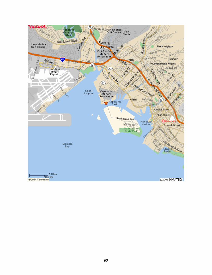
62

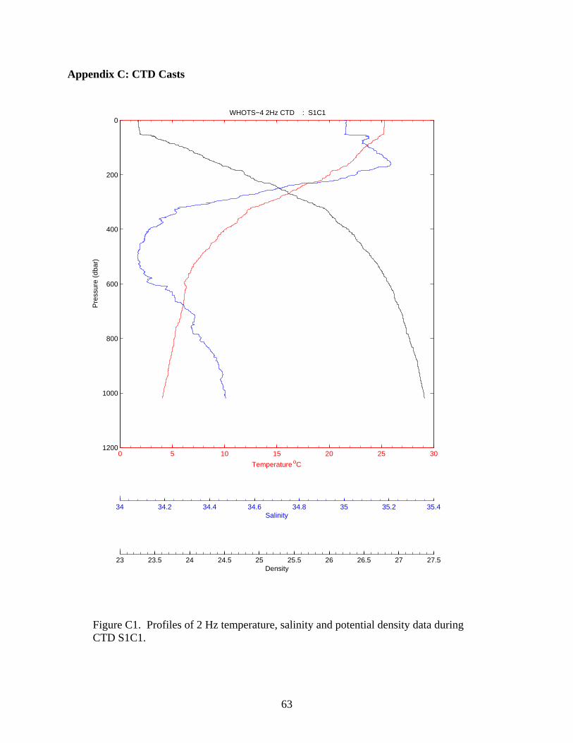
63

Appendix C: CTD Casts

0 5 10 15 20 25 30

0

200

400

600

800

1000

1200

Temperature oC

Pre

ssur

e (d

bar)

WHOTS−4 2Hz CTD : S1C1

34 34.2 34.4 34.6 34.8 35 35.2 35.4Salinity

23 23.5 24 24.5 25 25.5 26 26.5 27 27.5Density

Figure C1. Profiles of 2 Hz temperature, salinity and potential density data during CTD S1C1.

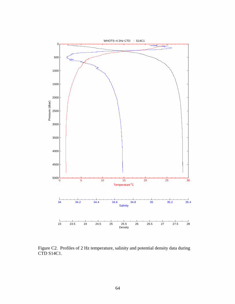
64

0 5 10 15 20 25 30

0

500

1000

1500

2000

2500

3000

3500

4000

4500

5000

Temperature oC

Pre

ssur

e (d

bar)

WHOTS−4 2Hz CTD : S14C1

34 34.2 34.4 34.6 34.8 35 35.2 35.4Salinity

23 23.5 24 24.5 25 25.5 26 26.5 27 27.5 28Density

Figure C2. Profiles of 2 Hz temperature, salinity and potential density data during CTD S14C1.

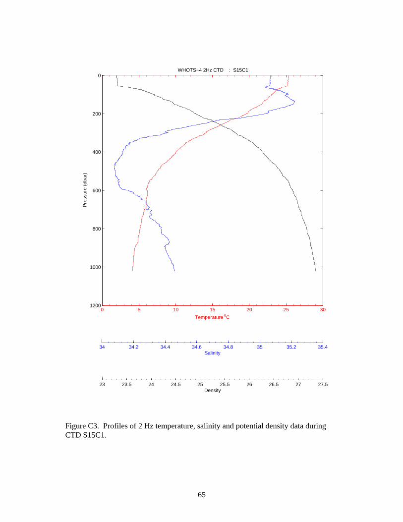
65

0 5 10 15 20 25 30

0

200

400

600

800

1000

1200

Temperature oC

Pre

ssur

e (d

bar)

WHOTS−4 2Hz CTD : S15C1

34 34.2 34.4 34.6 34.8 35 35.2 35.4Salinity

23 23.5 24 24.5 25 25.5 26 26.5 27 27.5Density

Figure C3. Profiles of 2 Hz temperature, salinity and potential density data during CTD S15C1.

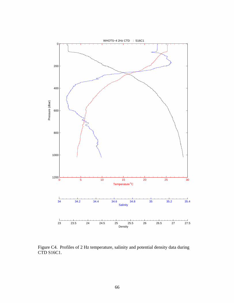
66

0 5 10 15 20 25 30

0

200

400

600

800

1000

1200

Temperature oC

Pre

ssur

e (d

bar)

WHOTS−4 2Hz CTD : S16C1

34 34.2 34.4 34.6 34.8 35 35.2 35.4Salinity

23 23.5 24 24.5 25 25.5 26 26.5 27 27.5Density

Figure C4. Profiles of 2 Hz temperature, salinity and potential density data during CTD S16C1.

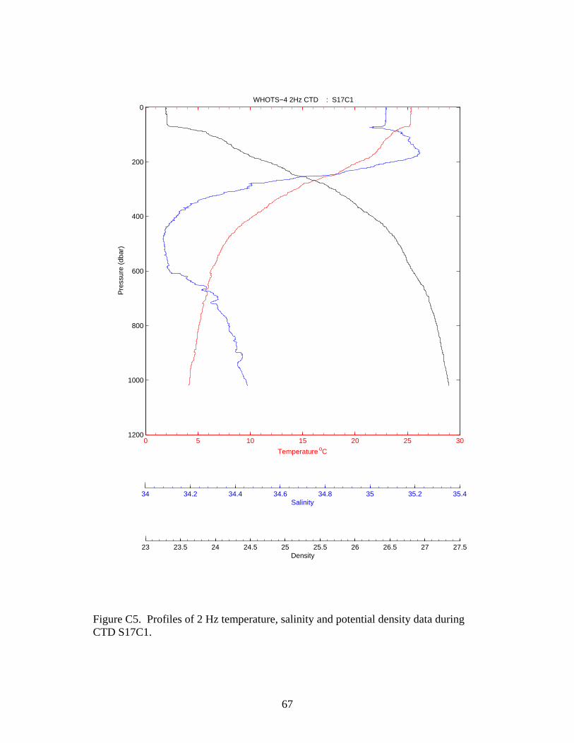
67

0 5 10 15 20 25 30

0

200

400

600

800

1000

1200

Temperature oC

Pre

ssur

e (d

bar)

WHOTS−4 2Hz CTD : S17C1

34 34.2 34.4 34.6 34.8 35 35.2 35.4Salinity

23 23.5 24 24.5 25 25.5 26 26.5 27 27.5Density

Figure C5. Profiles of 2 Hz temperature, salinity and potential density data during CTD S17C1.

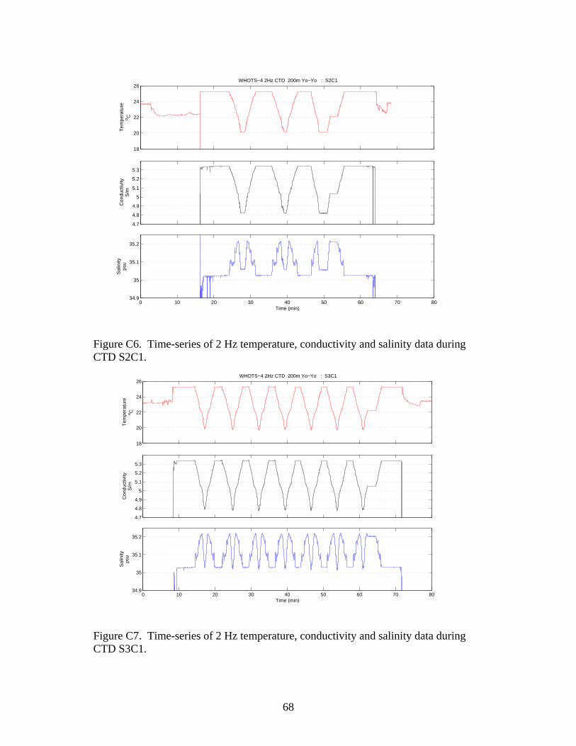
68

18

20

22

24

26WHOTS−4 2Hz CTD 200m Yo−Yo : S2C1

Tem

pera

ture

o C

4.7

4.8

4.9

5

5.1

5.2

5.3

Con

duct

ivity

S/m

0 10 20 30 40 50 60 70 8034.9

35

35.1

35.2

Sal

inity

psu

Time (min)

Figure C6. Time-series of 2 Hz temperature, conductivity and salinity data during CTD S2C1.

18

20

22

24

26WHOTS−4 2Hz CTD 200m Yo−Yo : S3C1

Tem

pera

ture

o C

4.7

4.8

4.9

5

5.1

5.2

5.3

Con

duct

ivity

S/m

0 10 20 30 40 50 60 70 8034.9

35

35.1

35.2

Sal

inity

psu

Time (min)

Figure C7. Time-series of 2 Hz temperature, conductivity and salinity data during CTD S3C1.

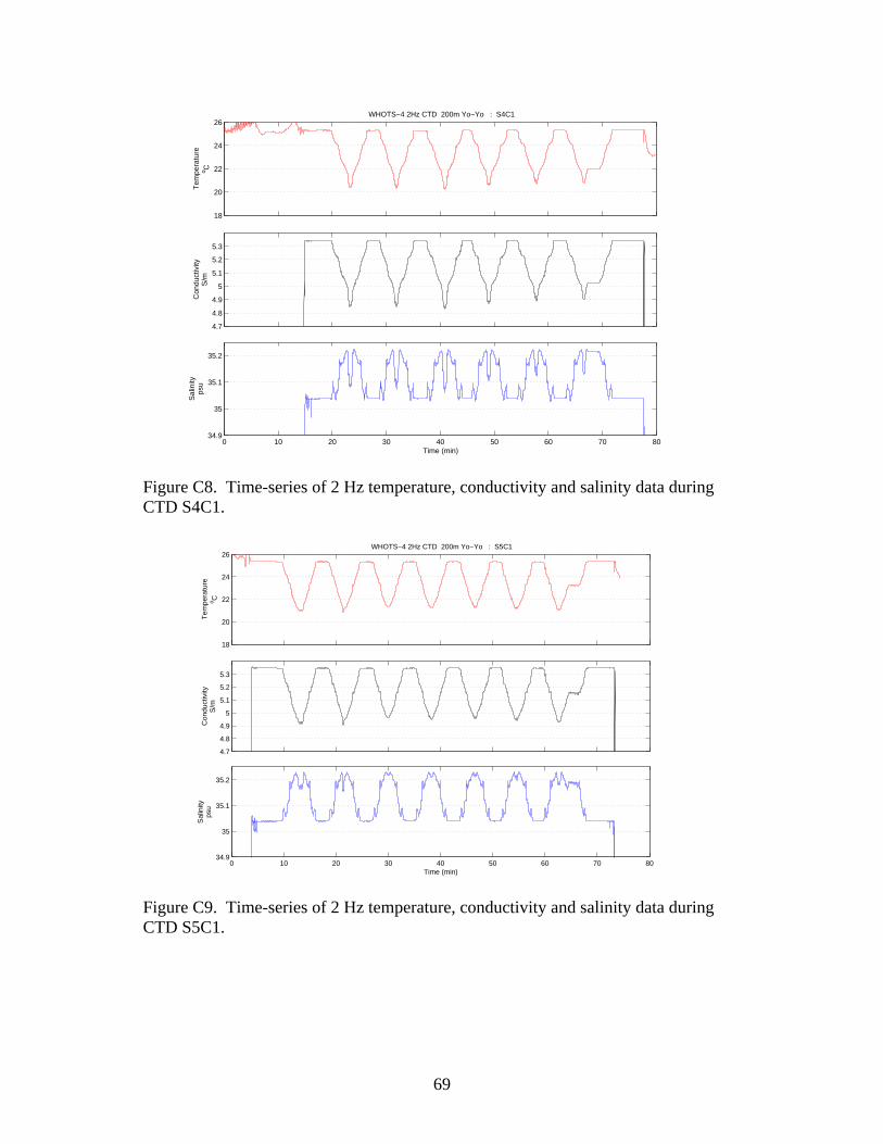
69

18

20

22

24

26WHOTS−4 2Hz CTD 200m Yo−Yo : S4C1

Tem

pera

ture

o C

4.7

4.8

4.9

5

5.1

5.2

5.3

Con

duct

ivity

S/m

0 10 20 30 40 50 60 70 8034.9

35

35.1

35.2

Sal

inity

psu

Time (min)

Figure C8. Time-series of 2 Hz temperature, conductivity and salinity data during CTD S4C1.

18

20

22

24

26WHOTS−4 2Hz CTD 200m Yo−Yo : S5C1

Tem

pera

ture

o C

4.7

4.8

4.9

5

5.1

5.2

5.3

Con

duct

ivity

S/m

0 10 20 30 40 50 60 70 8034.9

35

35.1

35.2

Sal

inity

psu

Time (min)

Figure C9. Time-series of 2 Hz temperature, conductivity and salinity data during CTD S5C1.

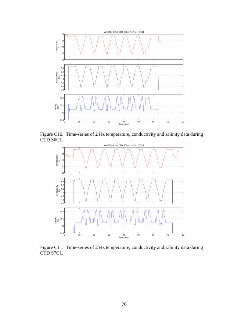
70

18

20

22

24

26WHOTS−4 2Hz CTD 200m Yo−Yo : S6C1

Tem

pera

ture

o C

4.7

4.8

4.9

5

5.1

5.2

5.3

Con

duct

ivity

S/m

0 10 20 30 40 50 60 70 8034.9

35

35.1

35.2

Sal

inity

psu

Time (min)

Figure C10. Time-series of 2 Hz temperature, conductivity and salinity data during CTD S6C1.

18

20

22

24

26WHOTS−4 2Hz CTD 200m Yo−Yo : S7C1

Tem

pera

ture

o C

4.7

4.8

4.9

5

5.1

5.2

5.3

Con

duct

ivity

S/m

0 10 20 30 40 50 60 70 8034.9

35

35.1

35.2

Sal

inity

psu

Time (min)

Figure C11. Time-series of 2 Hz temperature, conductivity and salinity data during CTD S7C1.

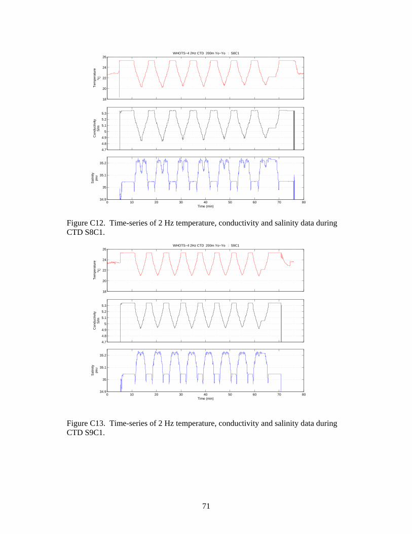
71

18

20

22

24

26WHOTS−4 2Hz CTD 200m Yo−Yo : S8C1

Tem

pera

ture

o C

4.7

4.8

4.9

5

5.1

5.2

5.3

Con

duct

ivity

S/m

0 10 20 30 40 50 60 70 8034.9

35

35.1

35.2

Sal

inity

psu

Time (min)

Figure C12. Time-series of 2 Hz temperature, conductivity and salinity data during CTD S8C1.

18

20

22

24

26WHOTS−4 2Hz CTD 200m Yo−Yo : S9C1

Tem

pera

ture

o C

4.7

4.8

4.9

5

5.1

5.2

5.3

Con

duct

ivity

S/m

0 10 20 30 40 50 60 70 8034.9

35

35.1

35.2

Sal

inity

psu

Time (min)

Figure C13. Time-series of 2 Hz temperature, conductivity and salinity data during CTD S9C1.

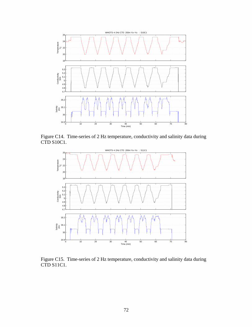
72

18

20

22

24

26WHOTS−4 2Hz CTD 200m Yo−Yo : S10C1

Tem

pera

ture

o C

4.7

4.8

4.9

5

5.1

5.2

5.3

Con

duct

ivity

S/m

0 10 20 30 40 50 60 70 8034.9

35

35.1

35.2

Sal

inity

psu

Time (min)

Figure C14. Time-series of 2 Hz temperature, conductivity and salinity data during CTD S10C1.

18

20

22

24

26WHOTS−4 2Hz CTD 200m Yo−Yo : S11C1

Tem

pera

ture

o C

4.7

4.8

4.9

5

5.1

5.2

5.3

Con

duct

ivity

S/m

0 10 20 30 40 50 60 70 8034.9

35

35.1

35.2

Sal

inity

psu

Time (min)

Figure C15. Time-series of 2 Hz temperature, conductivity and salinity data during CTD S11C1.

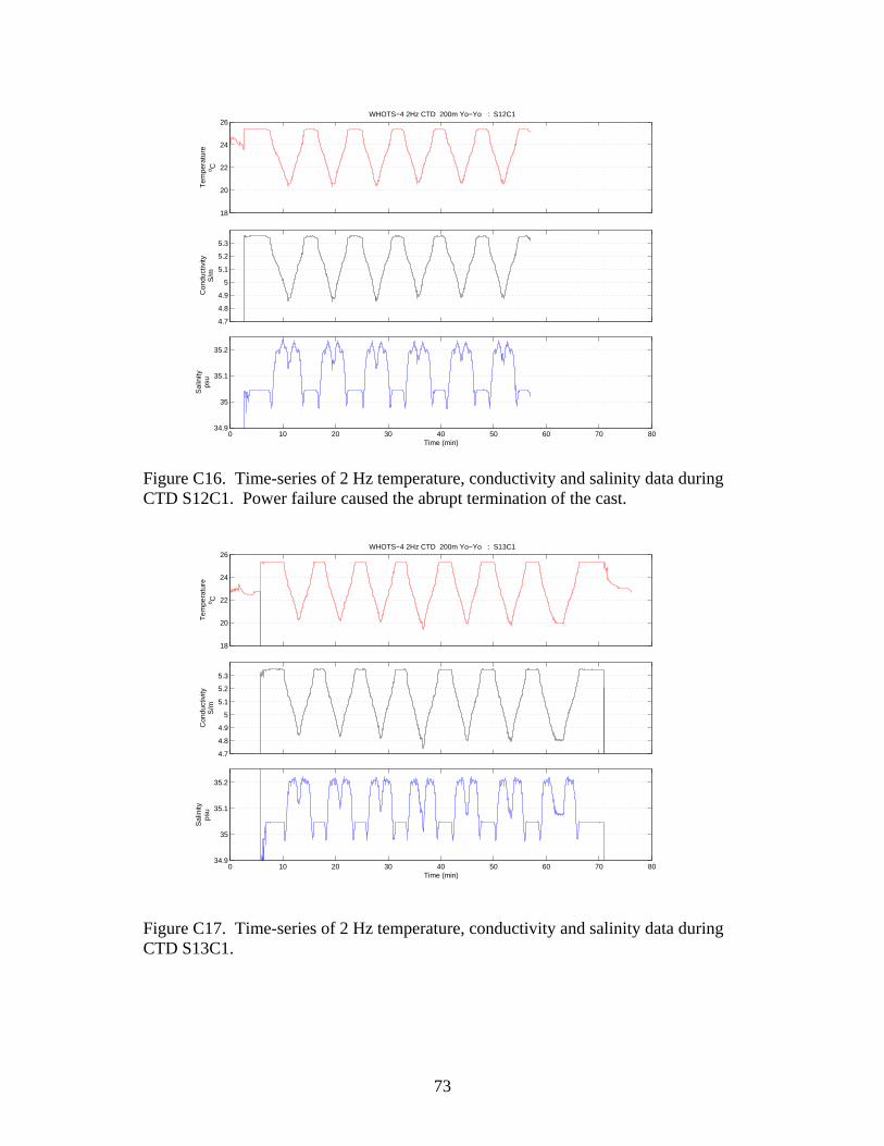
73

18

20

22

24

26WHOTS−4 2Hz CTD 200m Yo−Yo : S12C1

Tem

pera

ture

o C

4.7

4.8

4.9

5

5.1

5.2

5.3

Con

duct

ivity

S/m

0 10 20 30 40 50 60 70 8034.9

35

35.1

35.2

Sal

inity

psu

Time (min)

Figure C16. Time-series of 2 Hz temperature, conductivity and salinity data during CTD S12C1. Power failure caused the abrupt termination of the cast.

18

20

22

24

26WHOTS−4 2Hz CTD 200m Yo−Yo : S13C1

Tem

pera

ture

o C

4.7

4.8

4.9

5

5.1

5.2

5.3

Con

duct

ivity

S/m

0 10 20 30 40 50 60 70 8034.9

35

35.1

35.2

Sal

inity

psu

Time (min)

Figure C17. Time-series of 2 Hz temperature, conductivity and salinity data during CTD S13C1.

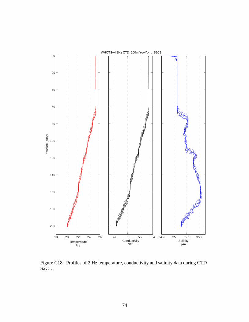
74

34.9 35 35.1 35.2Salinity

psu

4.8 5 5.2 5.4

WHOTS−4 2Hz CTD 200m Yo−Yo : S2C1

ConductivityS/m

18 20 22 24 26

0

20

40

60

80

100

120

140

160

180

200

TemperatureoC

Pre

ssur

e (d

bar)

Figure C18. Profiles of 2 Hz temperature, conductivity and salinity data during CTD S2C1.

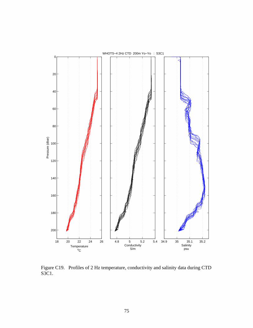
75

34.9 35 35.1 35.2Salinity

psu

4.8 5 5.2 5.4

WHOTS−4 2Hz CTD 200m Yo−Yo : S3C1

ConductivityS/m

18 20 22 24 26

0

20

40

60

80

100

120

140

160

180

200

TemperatureoC

Pre

ssur

e (d

bar)

Figure C19. Profiles of 2 Hz temperature, conductivity and salinity data during CTD S3C1.

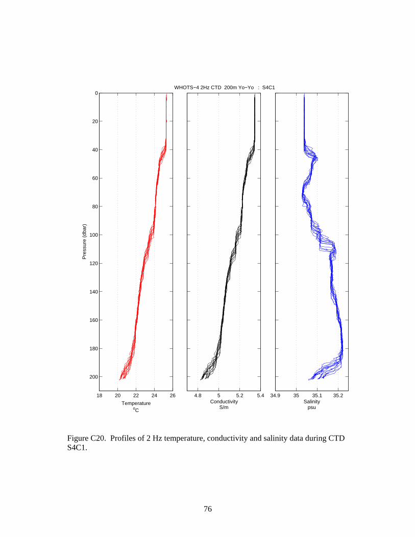
76

34.9 35 35.1 35.2Salinity

psu

4.8 5 5.2 5.4

WHOTS−4 2Hz CTD 200m Yo−Yo : S4C1

ConductivityS/m

18 20 22 24 26

0

20

40

60

80

100

120

140

160

180

200

TemperatureoC

Pre

ssur

e (d

bar)

Figure C20. Profiles of 2 Hz temperature, conductivity and salinity data during CTD S4C1.

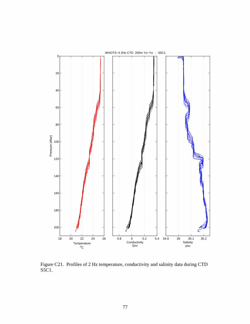
77

34.9 35 35.1 35.2Salinity

psu

4.8 5 5.2 5.4

WHOTS−4 2Hz CTD 200m Yo−Yo : S5C1

ConductivityS/m

18 20 22 24 26

0

20

40

60

80

100

120

140

160

180

200

TemperatureoC

Pre

ssur

e (d

bar)

Figure C21. Profiles of 2 Hz temperature, conductivity and salinity data during CTD S5C1.

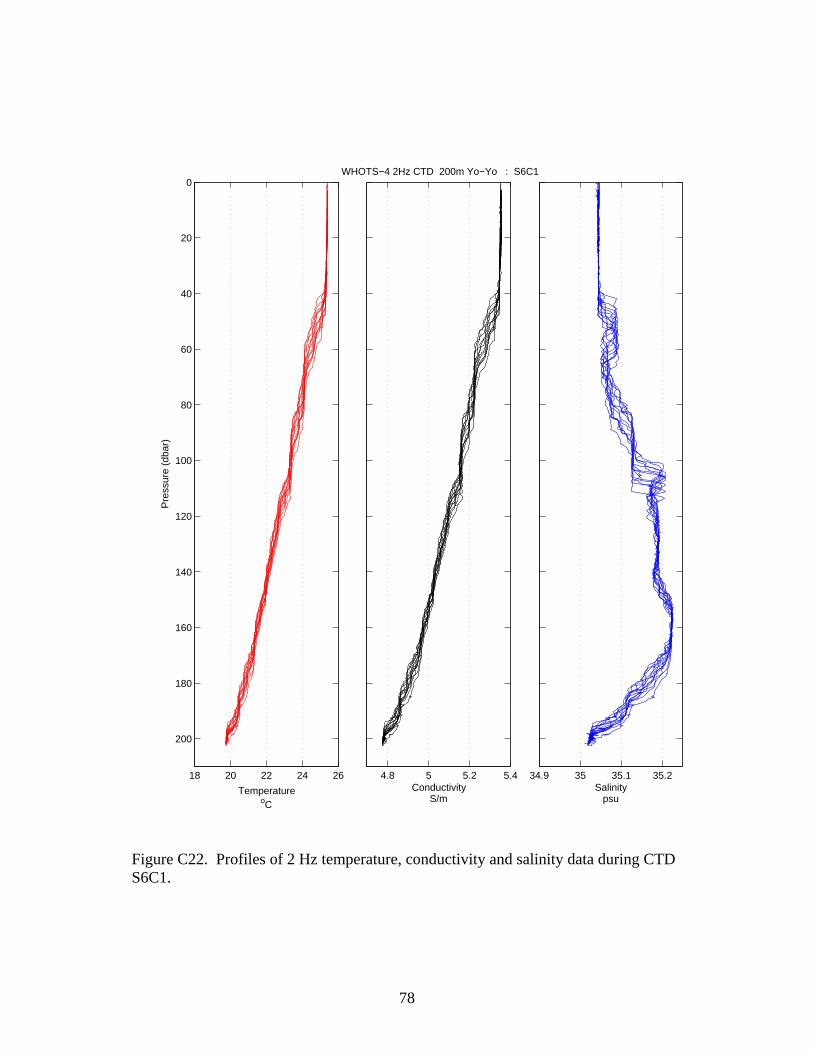
78

34.9 35 35.1 35.2Salinity

psu

4.8 5 5.2 5.4

WHOTS−4 2Hz CTD 200m Yo−Yo : S6C1

ConductivityS/m

18 20 22 24 26

0

20

40

60

80

100

120

140

160

180

200

TemperatureoC

Pre

ssur

e (d

bar)

Figure C22. Profiles of 2 Hz temperature, conductivity and salinity data during CTD S6C1.

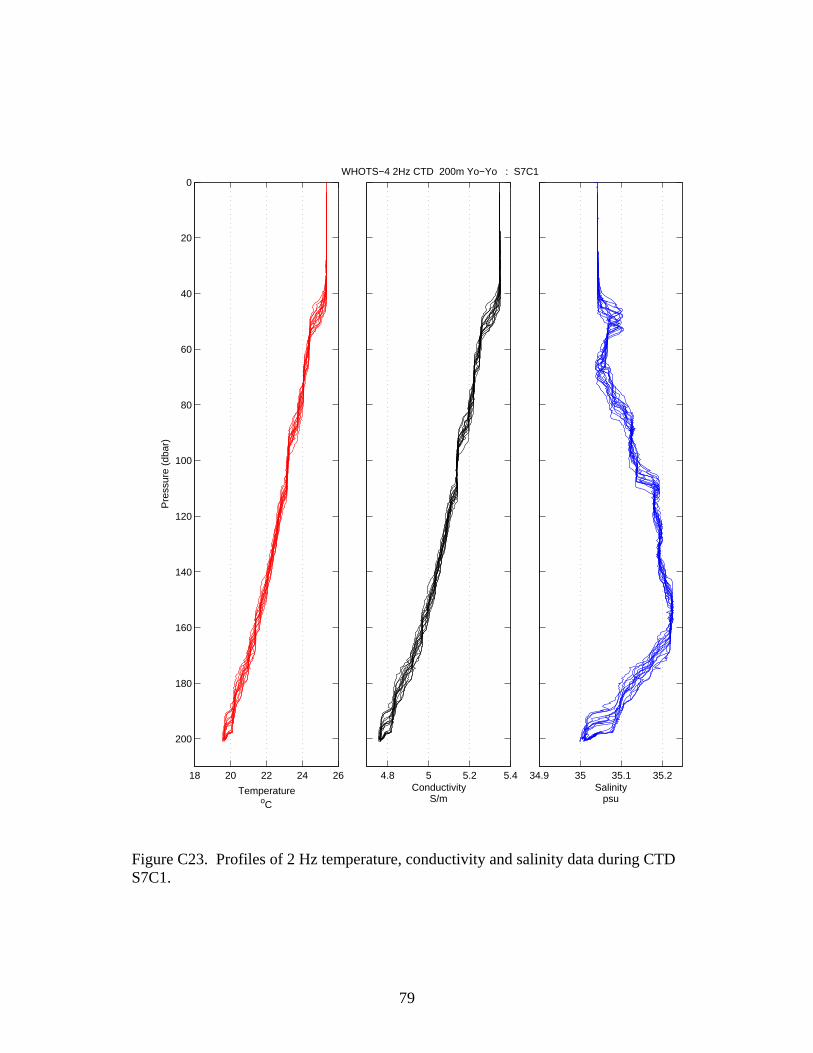
79

34.9 35 35.1 35.2Salinity

psu

4.8 5 5.2 5.4

WHOTS−4 2Hz CTD 200m Yo−Yo : S7C1

ConductivityS/m

18 20 22 24 26

0

20

40

60

80

100

120

140

160

180

200

TemperatureoC

Pre

ssur

e (d

bar)

Figure C23. Profiles of 2 Hz temperature, conductivity and salinity data during CTD S7C1.

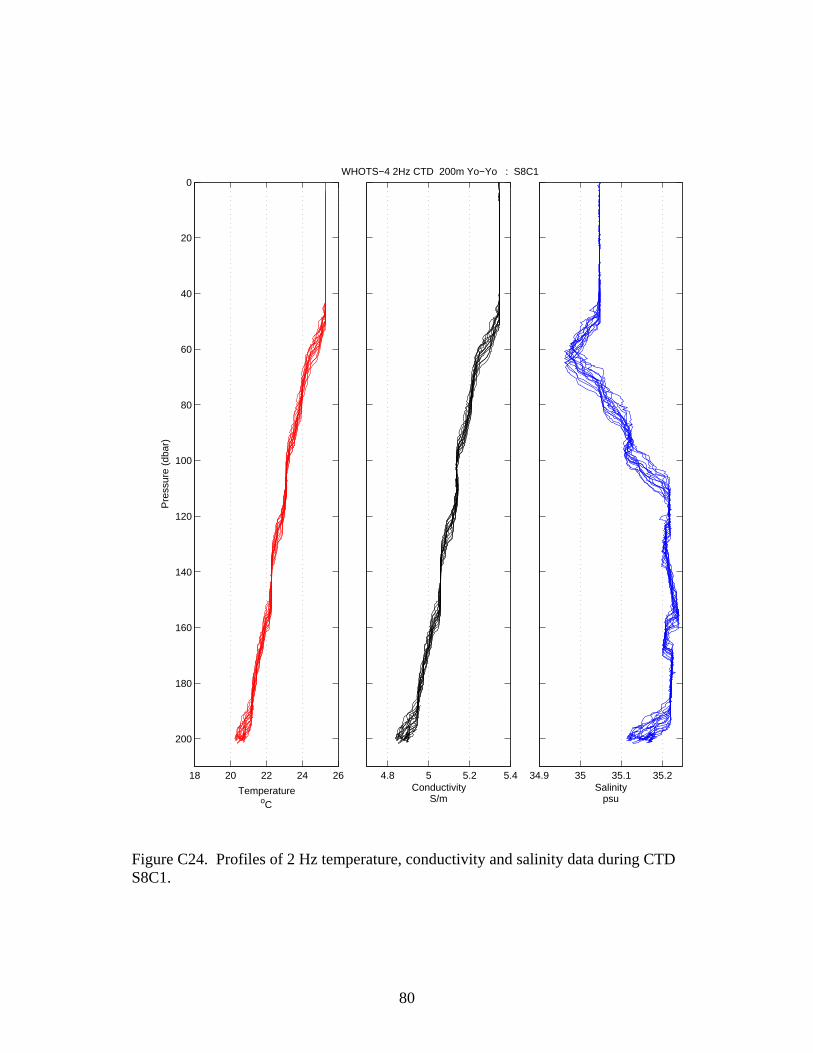
80

34.9 35 35.1 35.2Salinity

psu

4.8 5 5.2 5.4

WHOTS−4 2Hz CTD 200m Yo−Yo : S8C1

ConductivityS/m

18 20 22 24 26

0

20

40

60

80

100

120

140

160

180

200

TemperatureoC

Pre

ssur

e (d

bar)

Figure C24. Profiles of 2 Hz temperature, conductivity and salinity data during CTD S8C1.

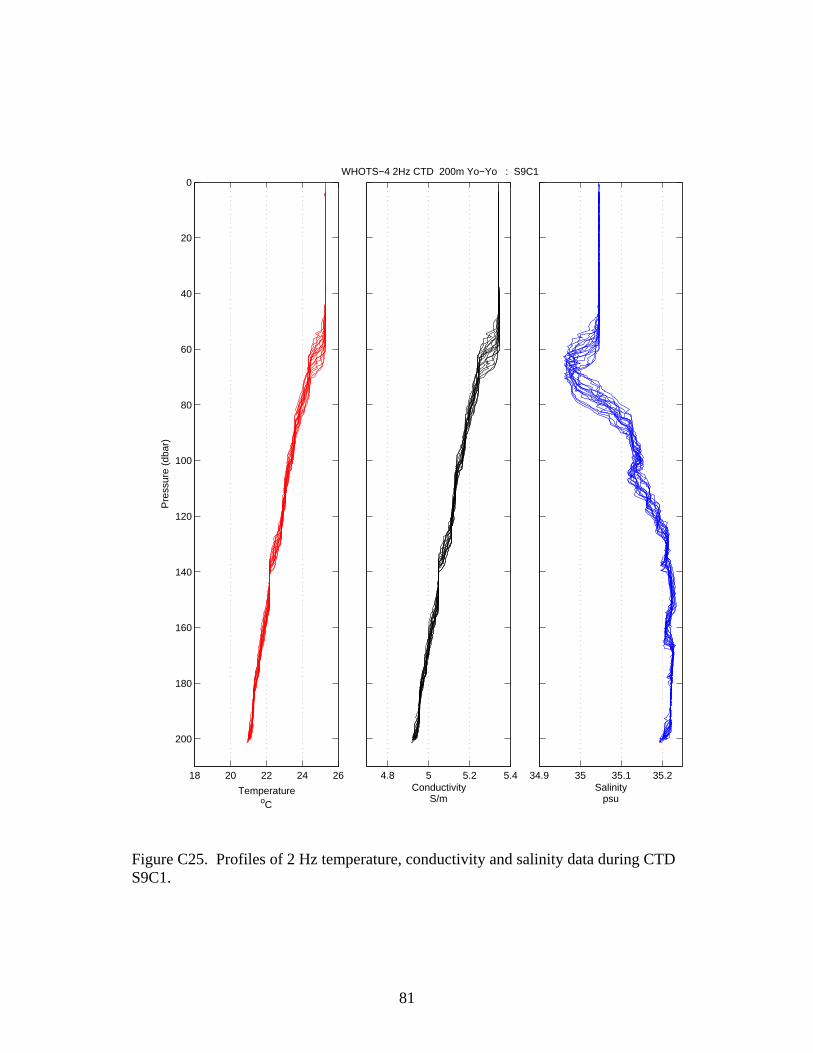
81

34.9 35 35.1 35.2Salinity

psu

4.8 5 5.2 5.4

WHOTS−4 2Hz CTD 200m Yo−Yo : S9C1

ConductivityS/m

18 20 22 24 26

0

20

40

60

80

100

120

140

160

180

200

TemperatureoC

Pre

ssur

e (d

bar)

Figure C25. Profiles of 2 Hz temperature, conductivity and salinity data during CTD S9C1.

82

34.9 35 35.1 35.2Salinity

psu

4.8 5 5.2 5.4

WHOTS−4 2Hz CTD 200m Yo−Yo : S10C1

ConductivityS/m

18 20 22 24 26

0

20

40

60

80

100

120

140

160

180

200

TemperatureoC

Pre

ssur

e (d

bar)

Figure C26. Profiles of 2 Hz temperature, conductivity and salinity data during CTD S10C1.

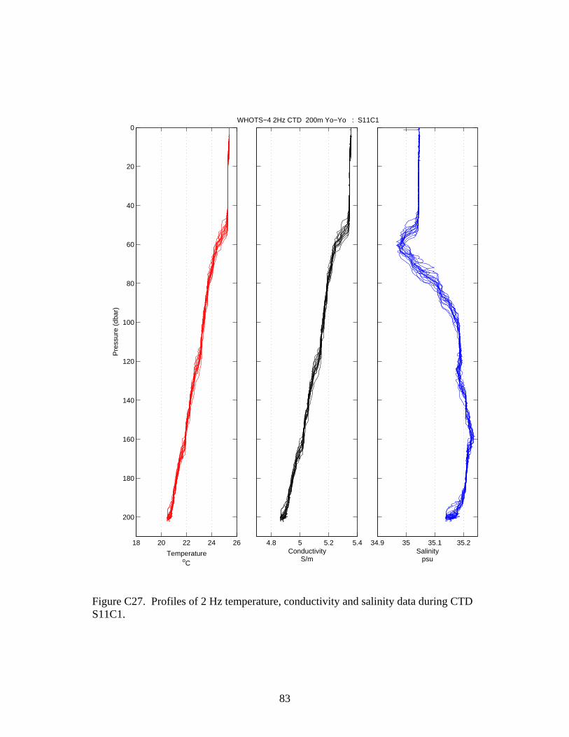
83

34.9 35 35.1 35.2Salinity

psu

4.8 5 5.2 5.4

WHOTS−4 2Hz CTD 200m Yo−Yo : S11C1

ConductivityS/m

18 20 22 24 26

0

20

40

60

80

100

120

140

160

180

200

TemperatureoC

Pre

ssur

e (d

bar)

Figure C27. Profiles of 2 Hz temperature, conductivity and salinity data during CTD S11C1.

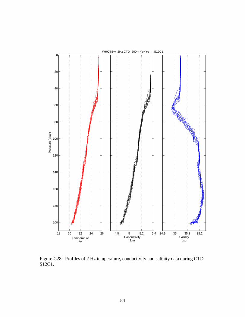
84

34.9 35 35.1 35.2Salinity

psu

4.8 5 5.2 5.4

WHOTS−4 2Hz CTD 200m Yo−Yo : S12C1

ConductivityS/m

18 20 22 24 26

0

20

40

60

80

100

120

140

160

180

200

TemperatureoC

Pre

ssur

e (d

bar)

Figure C28. Profiles of 2 Hz temperature, conductivity and salinity data during CTD S12C1.

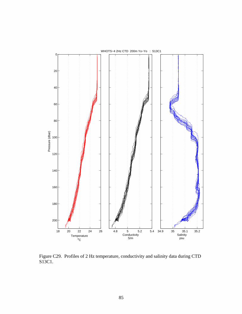
85

34.9 35 35.1 35.2Salinity

psu

4.8 5 5.2 5.4

WHOTS−4 2Hz CTD 200m Yo−Yo : S13C1

ConductivityS/m

18 20 22 24 26

0

20

40

60

80

100

120

140

160

180

200

TemperatureoC

Pre

ssur

e (d

bar)

Figure C29. Profiles of 2 Hz temperature, conductivity and salinity data during CTD S13C1.

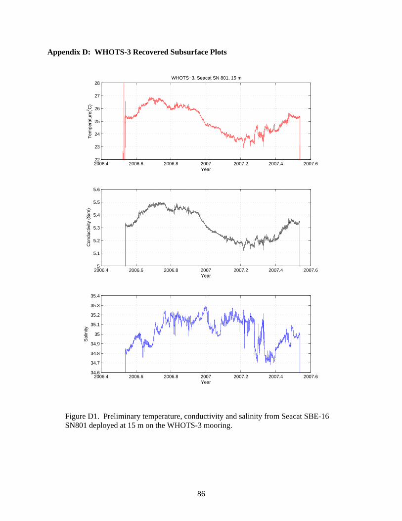
86

Appendix D: WHOTS-3 Recovered Subsurface Plots

2006.4 2006.6 2006.8 2007 2007.2 2007.4 2007.622

23

24

25

26

27

28

Year

Tem

pera

ture

(° C)

WHOTS−3, Seacat SN 801, 15 m

2006.4 2006.6 2006.8 2007 2007.2 2007.4 2007.65

5.1

5.2

5.3

5.4

5.5

5.6

Year

Con

duct

ivity

(S

/m)

2006.4 2006.6 2006.8 2007 2007.2 2007.4 2007.634.6

34.7

34.8

34.9

35

35.1

35.2

35.3

35.4

Year

Sal

inity

Figure D1. Preliminary temperature, conductivity and salinity from Seacat SBE-16 SN801 deployed at 15 m on the WHOTS-3 mooring.

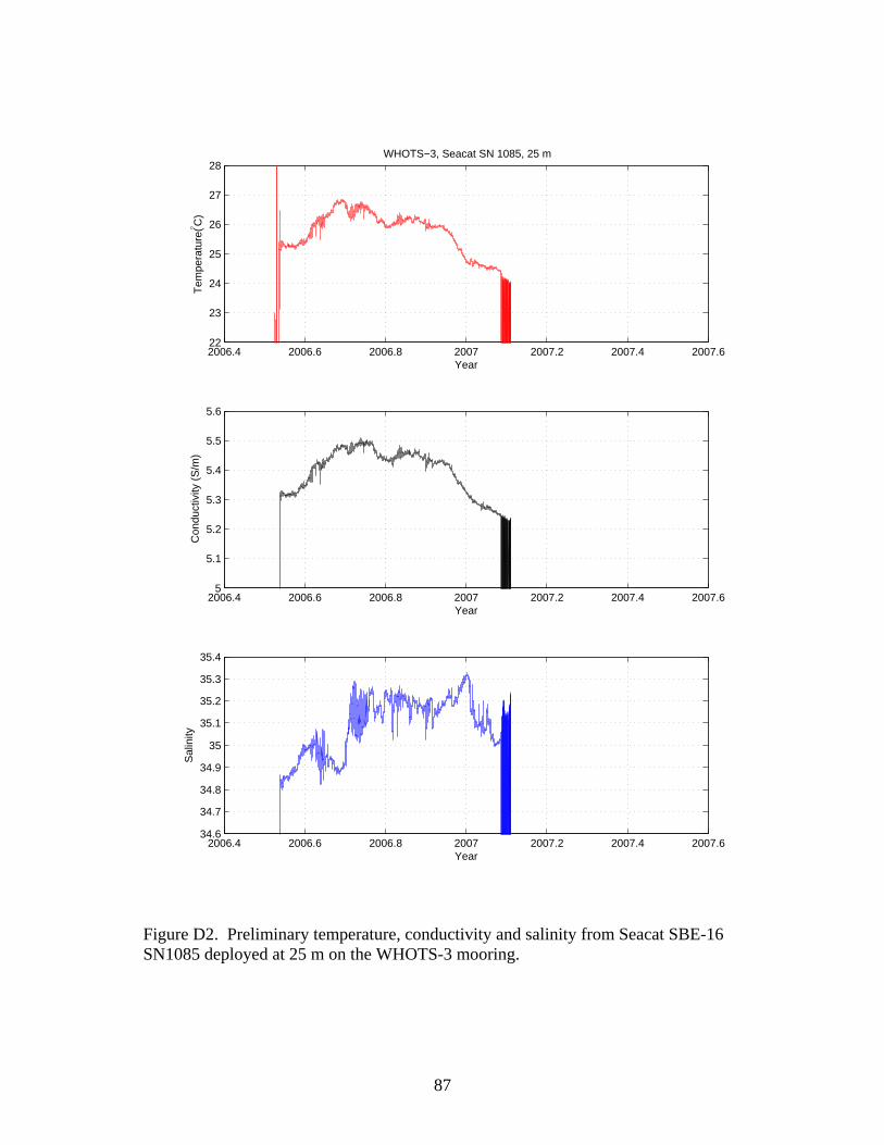
87

2006.4 2006.6 2006.8 2007 2007.2 2007.4 2007.622

23

24

25

26

27

28

Year

Tem

pera

ture

(° C)

WHOTS−3, Seacat SN 1085, 25 m

2006.4 2006.6 2006.8 2007 2007.2 2007.4 2007.65

5.1

5.2

5.3

5.4

5.5

5.6

Year

Con

duct

ivity

(S

/m)

2006.4 2006.6 2006.8 2007 2007.2 2007.4 2007.634.6

34.7

34.8

34.9

35

35.1

35.2

35.3

35.4

Year

Sal

inity

Figure D2. Preliminary temperature, conductivity and salinity from Seacat SBE-16 SN1085 deployed at 25 m on the WHOTS-3 mooring.

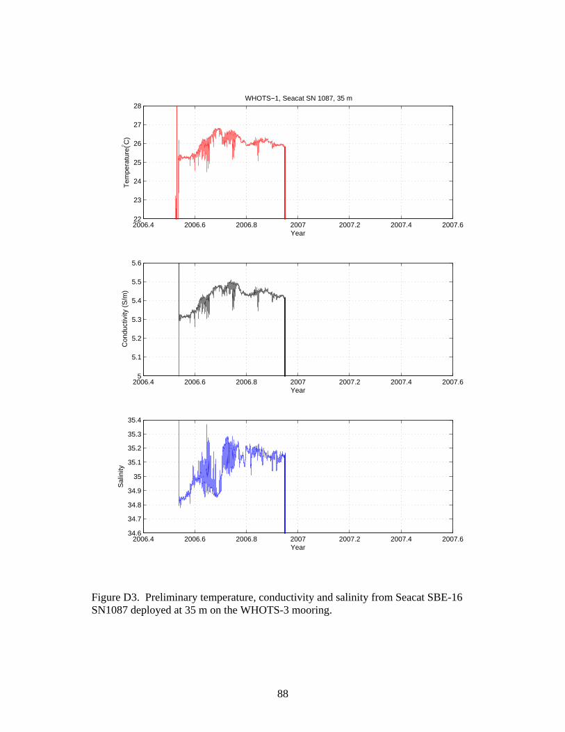
88

2006.4 2006.6 2006.8 2007 2007.2 2007.4 2007.622

23

24

25

26

27

28

Year

Tem

pera

ture

(° C)

WHOTS−1, Seacat SN 1087, 35 m

2006.4 2006.6 2006.8 2007 2007.2 2007.4 2007.65

5.1

5.2

5.3

5.4

5.5

5.6

Year

Con

duct

ivity

(S

/m)

2006.4 2006.6 2006.8 2007 2007.2 2007.4 2007.634.6

34.7

34.8

34.9

35

35.1

35.2

35.3

35.4

Year

Sal

inity

Figure D3. Preliminary temperature, conductivity and salinity from Seacat SBE-16 SN1087 deployed at 35 m on the WHOTS-3 mooring.

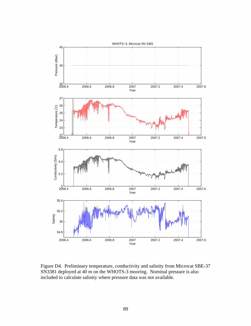
89

2006.4 2006.6 2006.8 2007 2007.2 2007.4 2007.635

40

45

Year

Pre

ssur

e (d

bar)

WHOTS−3, Microcat SN 3381

2006.4 2006.6 2006.8 2007 2007.2 2007.4 2007.622

23

24

25

26

27

Year

Tem

pera

ture

(° C)

2006.4 2006.6 2006.8 2007 2007.2 2007.4 2007.65

5.2

5.4

5.6

Year

Con

duct

ivity

(S

/m)

2006.4 2006.6 2006.8 2007 2007.2 2007.4 2007.6

34.8

35

35.2

35.4

Year

Sal

inity

Figure D4. Preliminary temperature, conductivity and salinity from Microcat SBE-37 SN3381 deployed at 40 m on the WHOTS-3 mooring. Nominal pressure is also included to calculate salinity where pressure data was not available.

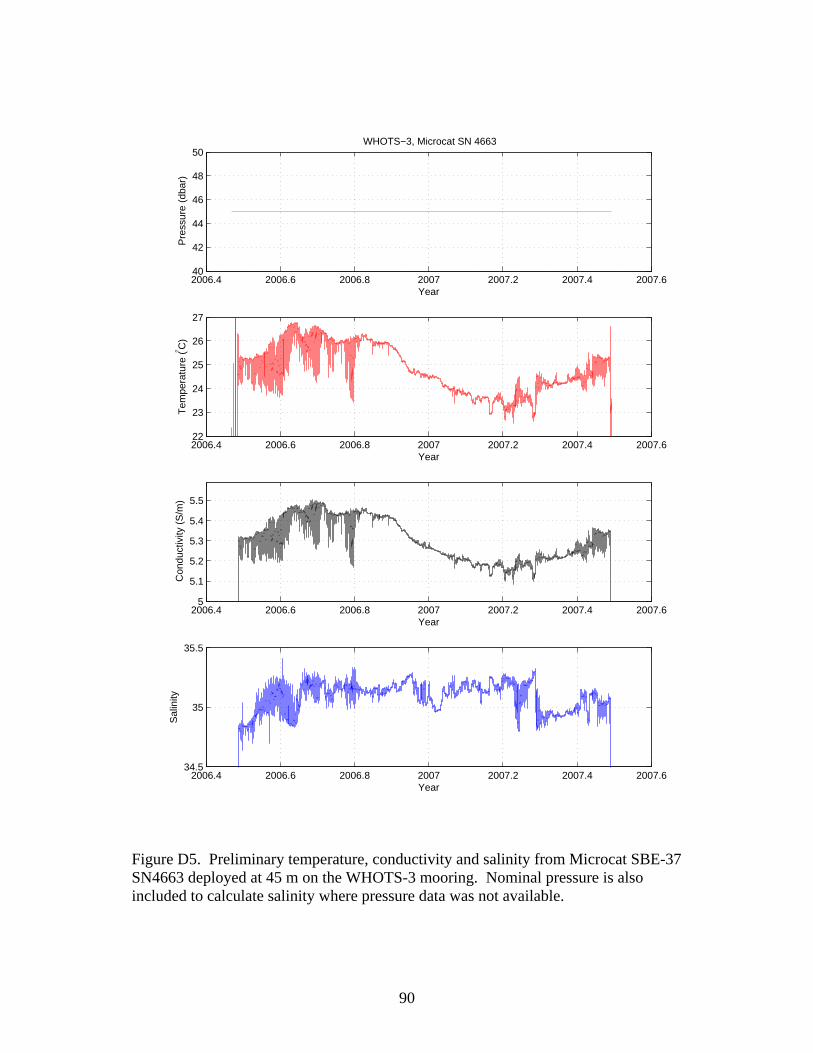
90

2006.4 2006.6 2006.8 2007 2007.2 2007.4 2007.640

42

44

46

48

50

Year

Pre

ssur

e (d

bar)

WHOTS−3, Microcat SN 4663

2006.4 2006.6 2006.8 2007 2007.2 2007.4 2007.622

23

24

25

26

27

Year

Tem

pera

ture

(° C)

2006.4 2006.6 2006.8 2007 2007.2 2007.4 2007.65

5.1

5.2

5.3

5.4

5.5

Year

Con

duct

ivity

(S

/m)

2006.4 2006.6 2006.8 2007 2007.2 2007.4 2007.634.5

35

35.5

Year

Sal

inity

Figure D5. Preliminary temperature, conductivity and salinity from Microcat SBE-37 SN4663 deployed at 45 m on the WHOTS-3 mooring. Nominal pressure is also included to calculate salinity where pressure data was not available.

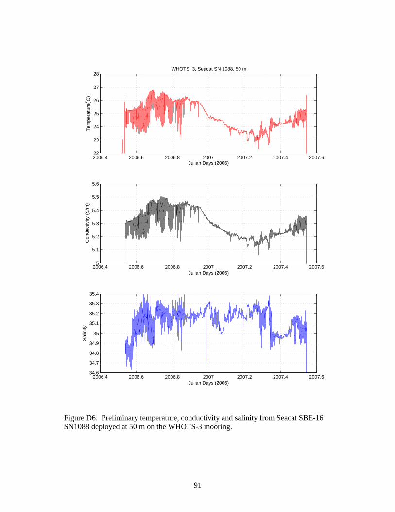
91

2006.4 2006.6 2006.8 2007 2007.2 2007.4 2007.622

23

24

25

26

27

28

Julian Days (2006)

Tem

pera

ture

(° C)

WHOTS−3, Seacat SN 1088, 50 m

2006.4 2006.6 2006.8 2007 2007.2 2007.4 2007.65

5.1

5.2

5.3

5.4

5.5

5.6

Julian Days (2006)

Con

duct

ivity

(S

/m)

2006.4 2006.6 2006.8 2007 2007.2 2007.4 2007.634.6

34.7

34.8

34.9

35

35.1

35.2

35.3

35.4

Julian Days (2006)

Sal

inity

Figure D6. Preliminary temperature, conductivity and salinity from Seacat SBE-16 SN1088 deployed at 50 m on the WHOTS-3 mooring.

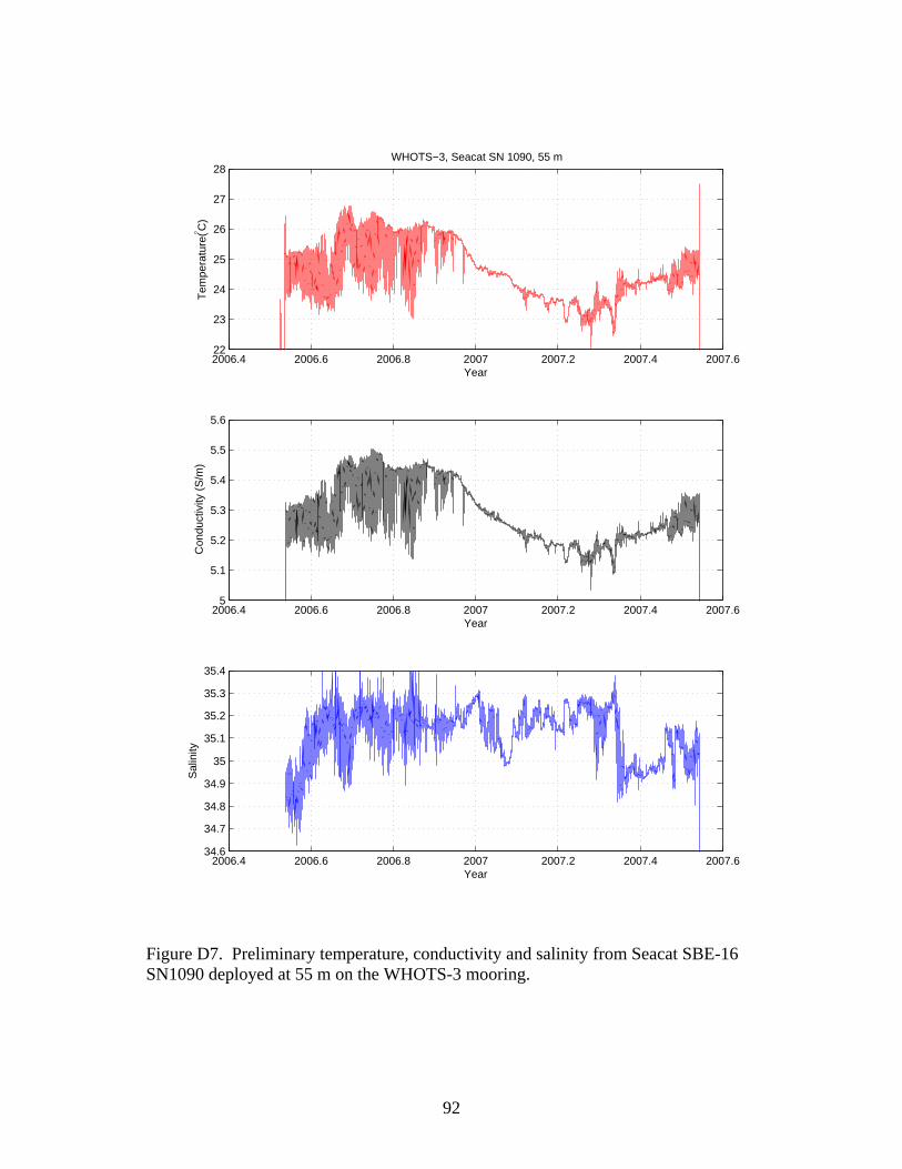
92

2006.4 2006.6 2006.8 2007 2007.2 2007.4 2007.622

23

24

25

26

27

28

Year

Tem

pera

ture

(° C)

WHOTS−3, Seacat SN 1090, 55 m

2006.4 2006.6 2006.8 2007 2007.2 2007.4 2007.65

5.1

5.2

5.3

5.4

5.5

5.6

Year

Con

duct

ivity

(S

/m)

2006.4 2006.6 2006.8 2007 2007.2 2007.4 2007.634.6

34.7

34.8

34.9

35

35.1

35.2

35.3

35.4

Year

Sal

inity

Figure D7. Preliminary temperature, conductivity and salinity from Seacat SBE-16 SN1090 deployed at 55 m on the WHOTS-3 mooring.

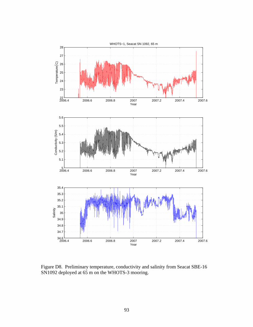
93

2006.4 2006.6 2006.8 2007 2007.2 2007.4 2007.622

23

24

25

26

27

28

Year

Tem

pera

ture

(° C)

WHOTS−1, Seacat SN 1092, 65 m

2006.4 2006.6 2006.8 2007 2007.2 2007.4 2007.65

5.1

5.2

5.3

5.4

5.5

5.6

Year

Con

duct

ivity

(S

/m)

2006.4 2006.6 2006.8 2007 2007.2 2007.4 2007.634.6

34.7

34.8

34.9

35

35.1

35.2

35.3

35.4

Year

Sal

inity

Figure D8. Preliminary temperature, conductivity and salinity from Seacat SBE-16 SN1092 deployed at 65 m on the WHOTS-3 mooring.

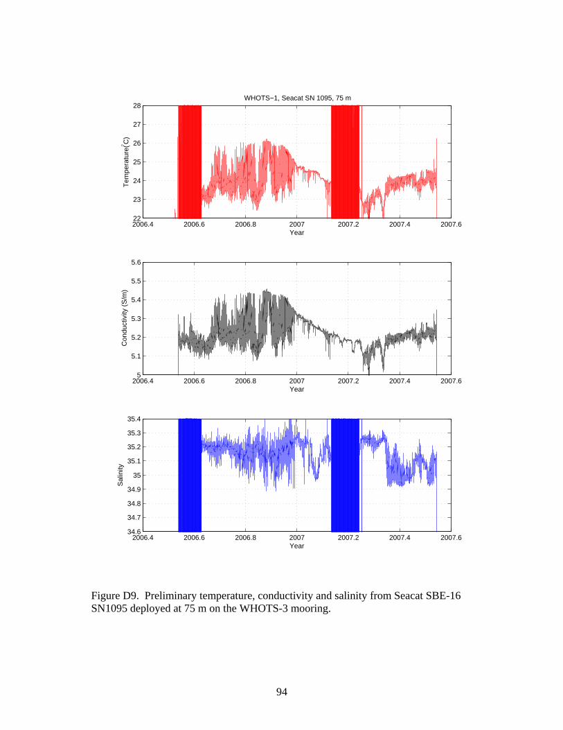
94

2006.4 2006.6 2006.8 2007 2007.2 2007.4 2007.622

23

24

25

26

27

28

Year

Tem

pera

ture

(° C)

WHOTS−1, Seacat SN 1095, 75 m

2006.4 2006.6 2006.8 2007 2007.2 2007.4 2007.65

5.1

5.2

5.3

5.4

5.5

5.6

Year

Con

duct

ivity

(S

/m)

2006.4 2006.6 2006.8 2007 2007.2 2007.4 2007.634.6

34.7

34.8

34.9

35

35.1

35.2

35.3

35.4

Year

Sal

inity

Figure D9. Preliminary temperature, conductivity and salinity from Seacat SBE-16 SN1095 deployed at 75 m on the WHOTS-3 mooring.

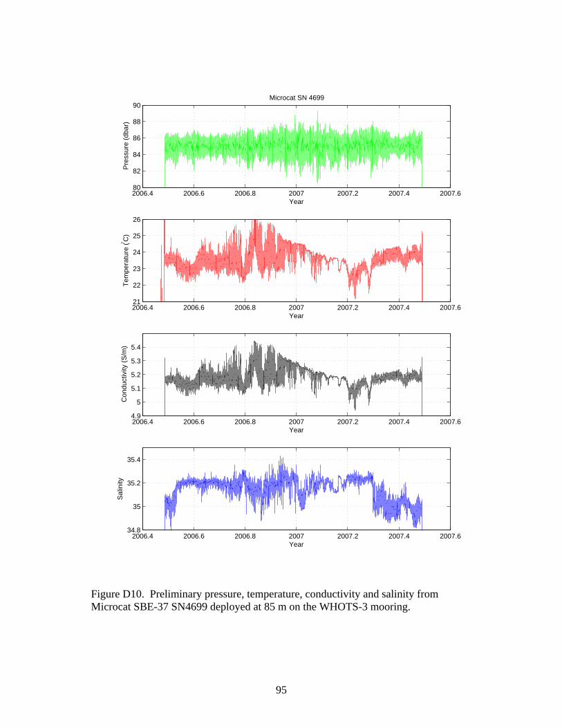
95

2006.4 2006.6 2006.8 2007 2007.2 2007.4 2007.680

82

84

86

88

90

Year

Pre

ssur

e (d

bar)

Microcat SN 4699

2006.4 2006.6 2006.8 2007 2007.2 2007.4 2007.621

22

23

24

25

26

Year

Tem

pera

ture

(° C)

2006.4 2006.6 2006.8 2007 2007.2 2007.4 2007.64.9

5

5.1

5.2

5.3

5.4

Year

Con

duct

ivity

(S

/m)

2006.4 2006.6 2006.8 2007 2007.2 2007.4 2007.634.8

35

35.2

35.4

Year

Sal

inity

Figure D10. Preliminary pressure, temperature, conductivity and salinity from Microcat SBE-37 SN4699 deployed at 85 m on the WHOTS-3 mooring.

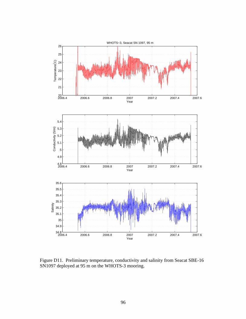
96

2006.4 2006.6 2006.8 2007 2007.2 2007.4 2007.620

21

22

23

24

25

26

Year

Tem

pera

ture

(° C)

WHOTS−3, Seacat SN 1097, 95 m

2006.4 2006.6 2006.8 2007 2007.2 2007.4 2007.64.8

4.9

5

5.1

5.2

5.3

5.4

Year

Con

duct

ivity

(S

/m)

2006.4 2006.6 2006.8 2007 2007.2 2007.4 2007.634.8

34.9

35

35.1

35.2

35.3

35.4

35.5

35.6

Year

Sal

inity

Figure D11. Preliminary temperature, conductivity and salinity from Seacat SBE-16 SN1097 deployed at 95 m on the WHOTS-3 mooring.

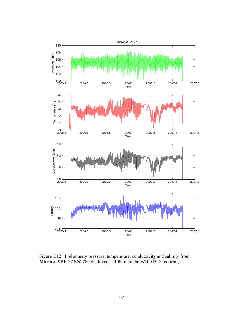
97

2006.4 2006.6 2006.8 2007 2007.2 2007.4 2007.6100

102

104

106

108

110

Year

Pre

ssur

e (d

bar)

Microcat SN 2769

2006.4 2006.6 2006.8 2007 2007.2 2007.4 2007.620

21

22

23

24

25

Year

Tem

pera

ture

(° C)

2006.4 2006.6 2006.8 2007 2007.2 2007.4 2007.64.8

5

5.2

5.4

Year

Con

duct

ivity

(S

/m)

2006.4 2006.6 2006.8 2007 2007.2 2007.4 2007.634.8

35

35.2

35.4

Year

Sal

inity

Figure D12. Preliminary pressure, temperature, conductivity and salinity from Microcat SBE-37 SN2769 deployed at 105 m on the WHOTS-3 mooring.

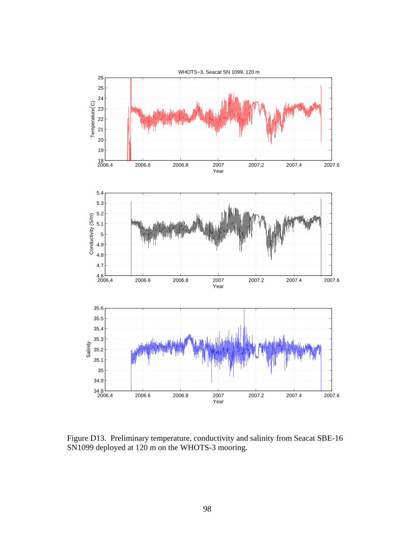
98

2006.4 2006.6 2006.8 2007 2007.2 2007.4 2007.618

19

20

21

22

23

24

25

26

Year

Tem

pera

ture

(° C)

WHOTS−3, Seacat SN 1099, 120 m

2006.4 2006.6 2006.8 2007 2007.2 2007.4 2007.64.6

4.7

4.8

4.9

5

5.1

5.2

5.3

5.4

Year

Con

duct

ivity

(S

/m)

2006.4 2006.6 2006.8 2007 2007.2 2007.4 2007.634.8

34.9

35

35.1

35.2

35.3

35.4

35.5

35.6

Year

Sal

inity

Figure D13. Preliminary temperature, conductivity and salinity from Seacat SBE-16 SN1099 deployed at 120 m on the WHOTS-3 mooring.

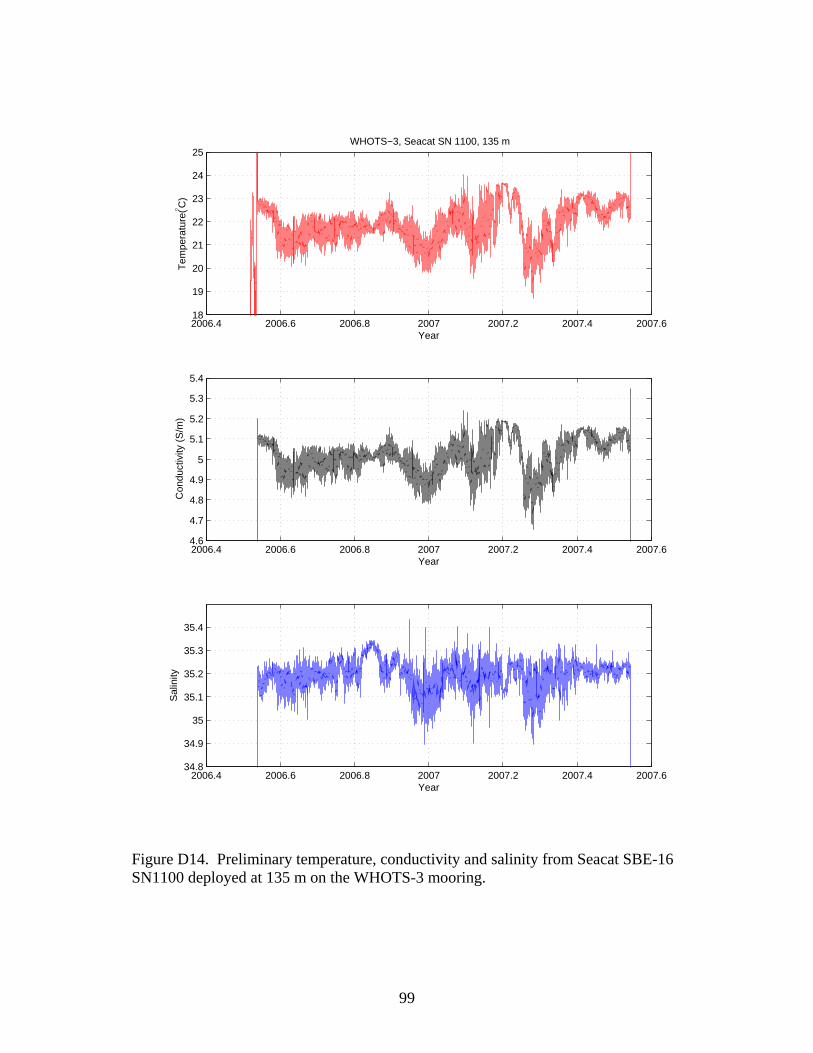
99

2006.4 2006.6 2006.8 2007 2007.2 2007.4 2007.618

19

20

21

22

23

24

25

Year

Tem

pera

ture

(° C)

WHOTS−3, Seacat SN 1100, 135 m

2006.4 2006.6 2006.8 2007 2007.2 2007.4 2007.64.6

4.7

4.8

4.9

5

5.1

5.2

5.3

5.4

Year

Con

duct

ivity

(S

/m)

2006.4 2006.6 2006.8 2007 2007.2 2007.4 2007.634.8

34.9

35

35.1

35.2

35.3

35.4

Year

Sal

inity

Figure D14. Preliminary temperature, conductivity and salinity from Seacat SBE-16 SN1100 deployed at 135 m on the WHOTS-3 mooring.

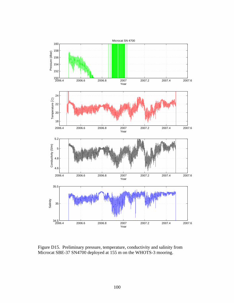
100

2006.4 2006.6 2006.8 2007 2007.2 2007.4 2007.6150

152

154

156

158

160

Year

Pre

ssur

e (d

bar)

Microcat SN 4700

2006.4 2006.6 2006.8 2007 2007.2 2007.4 2007.6

18

20

22

24

Year

Tem

pera

ture

(° C)

2006.4 2006.6 2006.8 2007 2007.2 2007.4 2007.6

4.6

4.8

5

5.2

Year

Con

duct

ivity

(S

/m)

2006.4 2006.6 2006.8 2007 2007.2 2007.4 2007.634.5

35

35.5

Year

Sal

inity

Figure D15. Preliminary pressure, temperature, conductivity and salinity from Microcat SBE-37 SN4700 deployed at 155 m on the WHOTS-3 mooring.

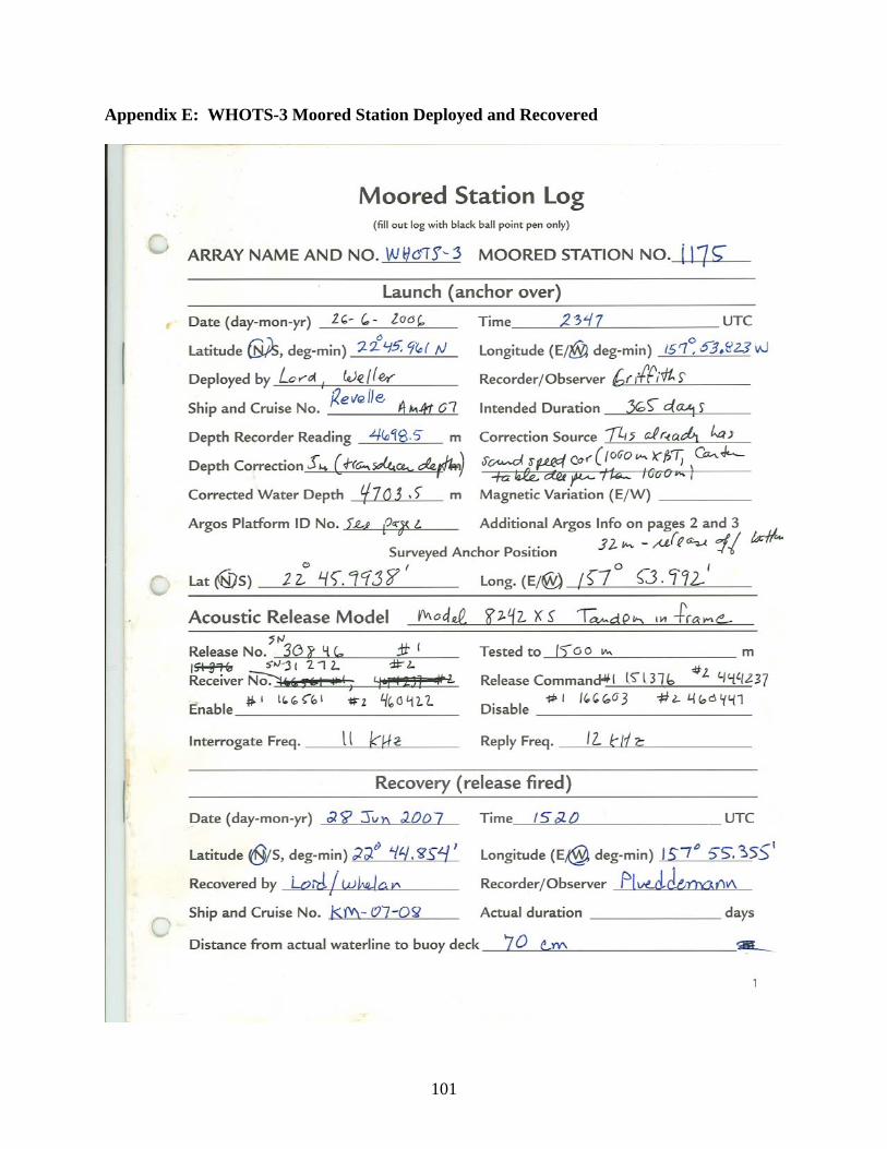
101

Appendix E: WHOTS-3 Moored Station Deployed and Recovered

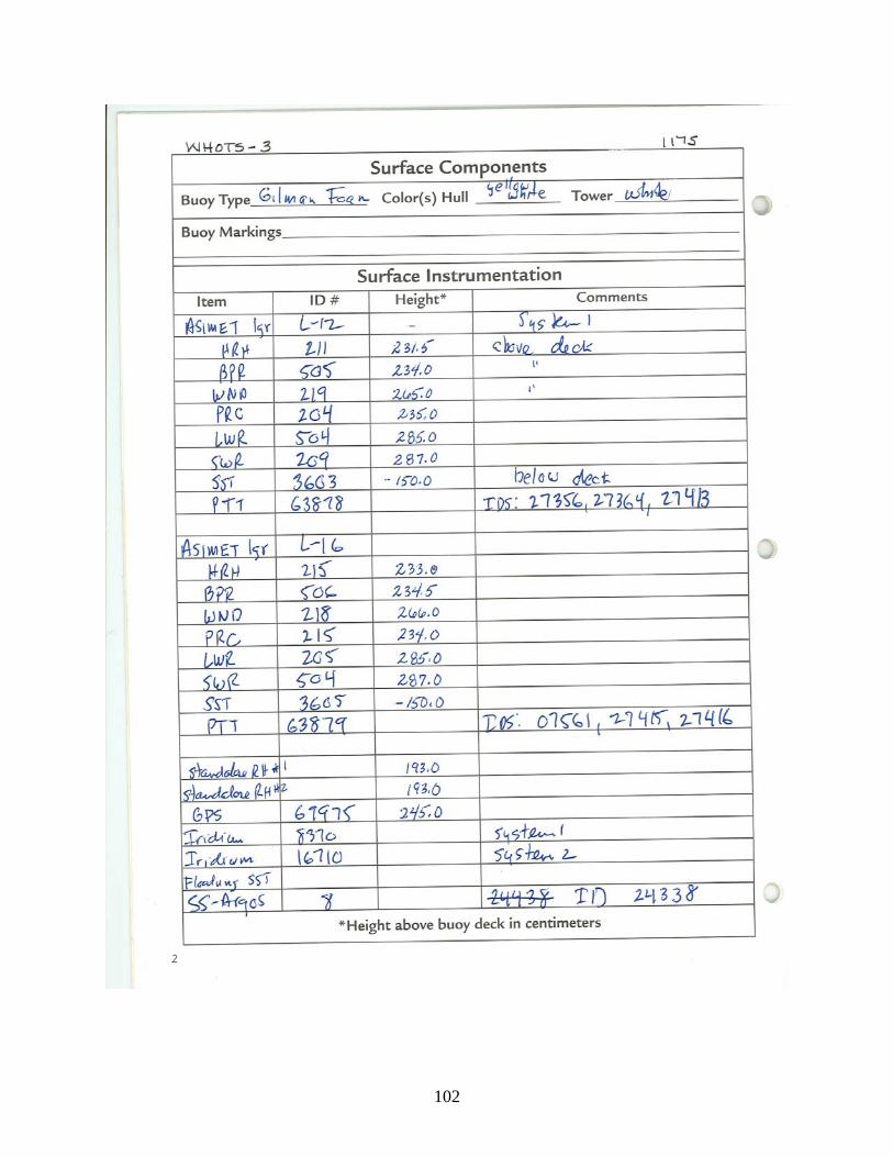
102

103

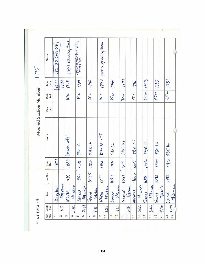
104

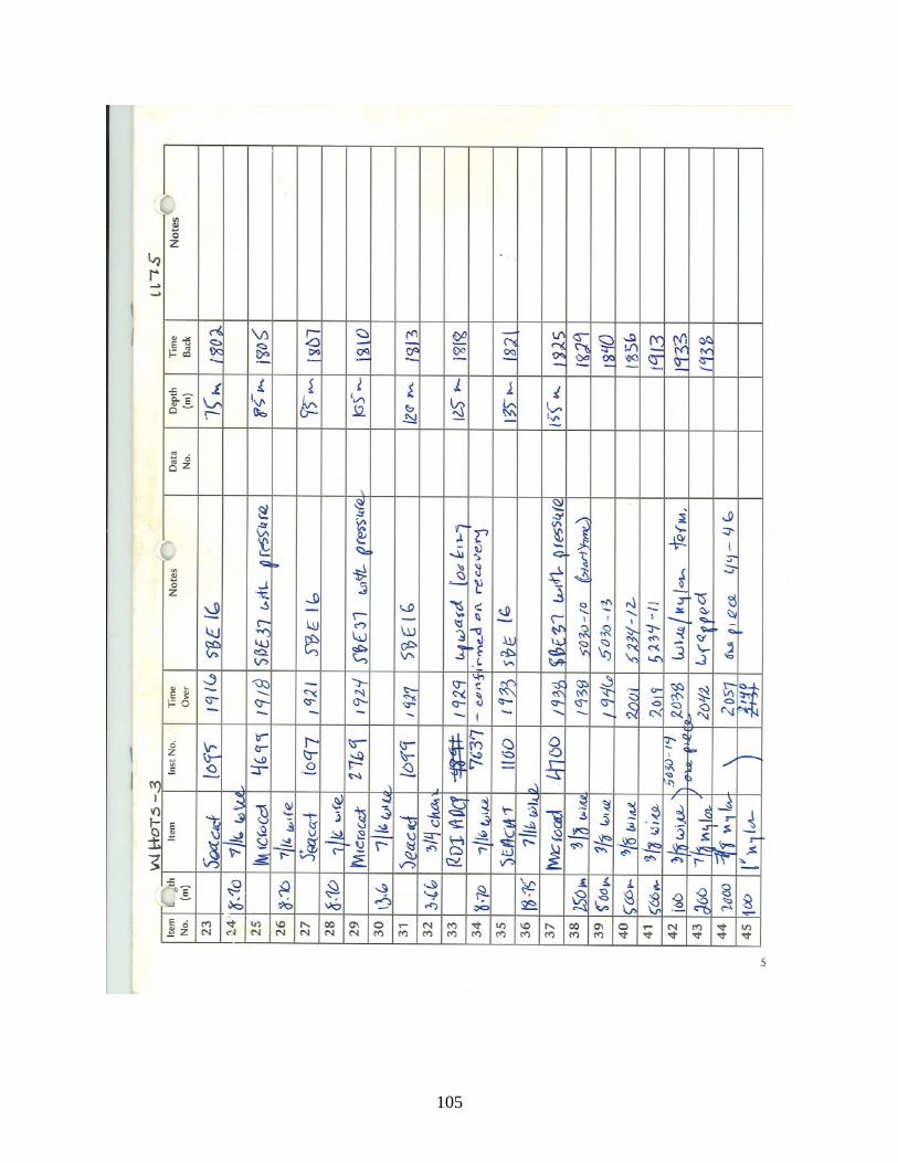
105

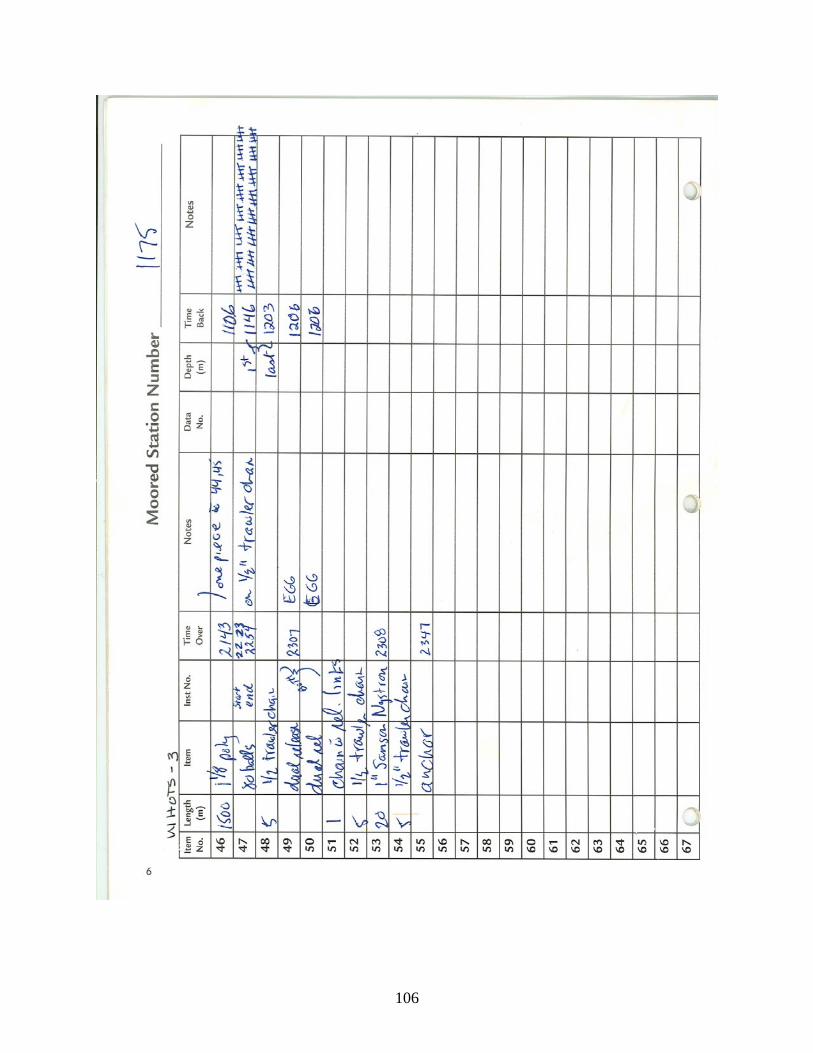
106

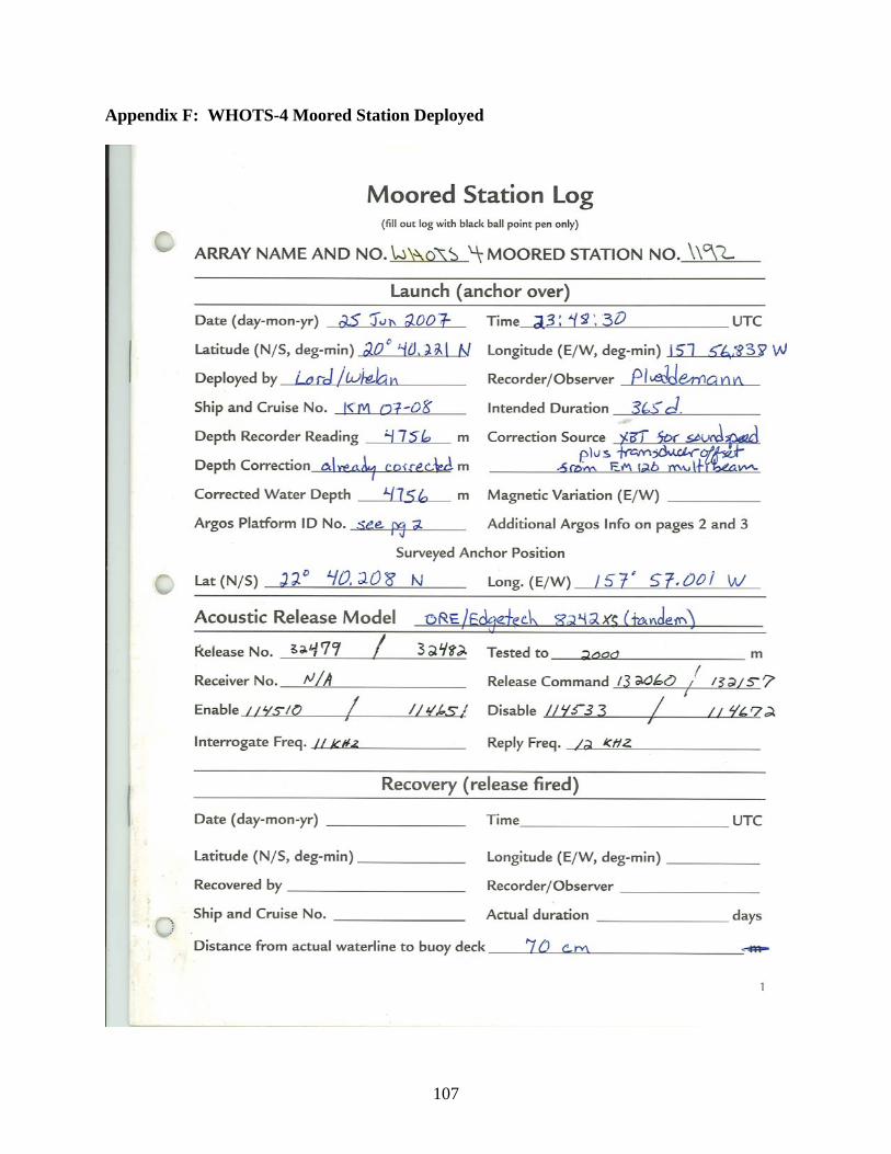
107

Appendix F: WHOTS-4 Moored Station Deployed

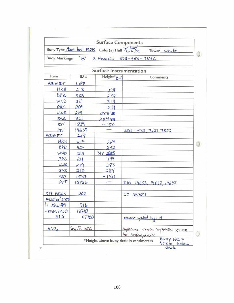
108

109

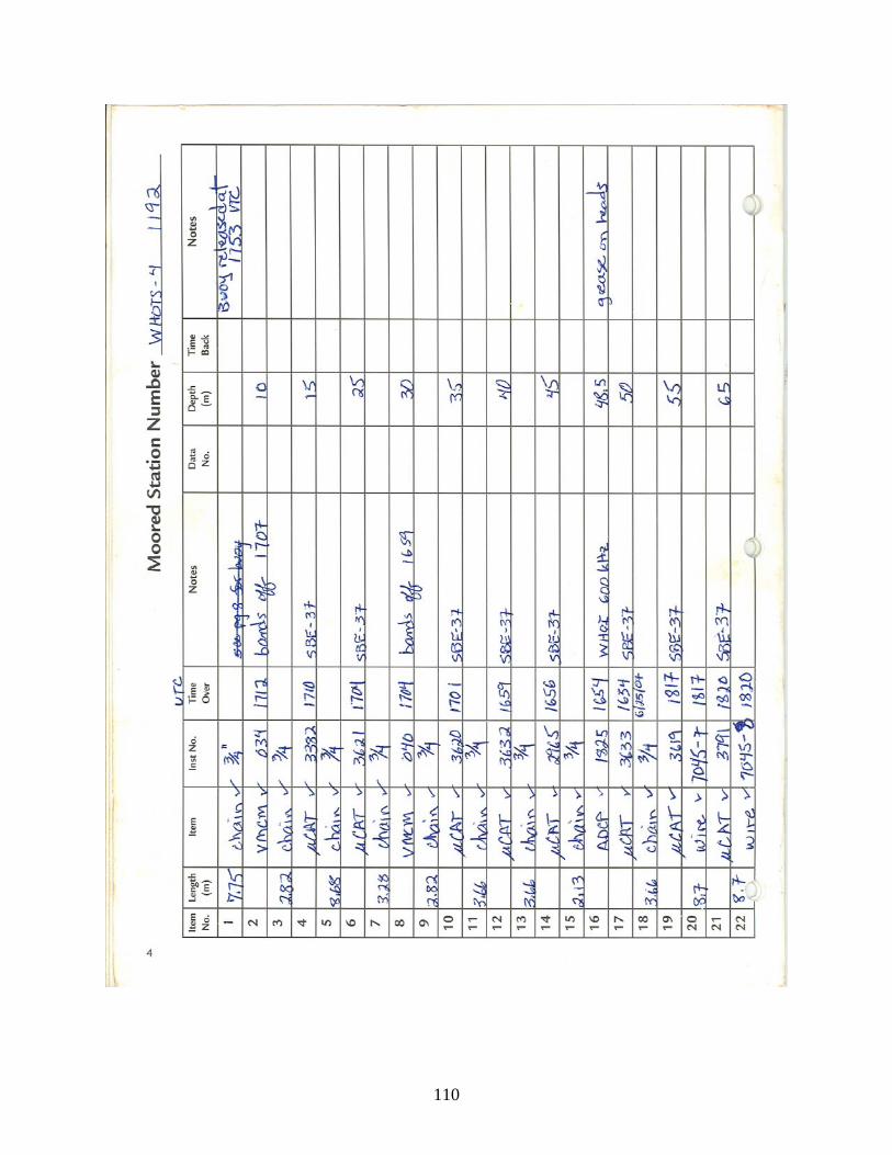
110

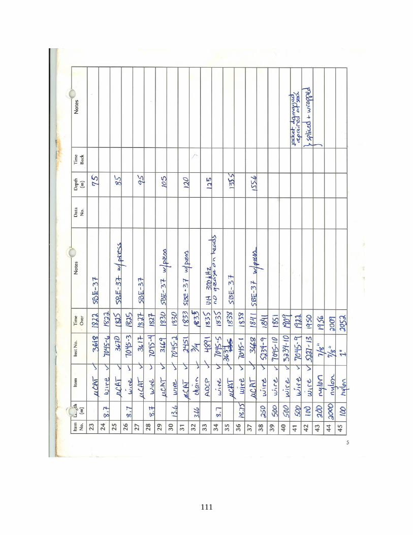
111

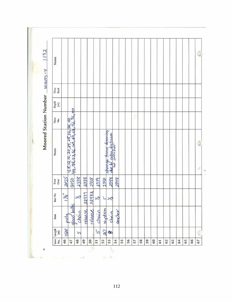
112

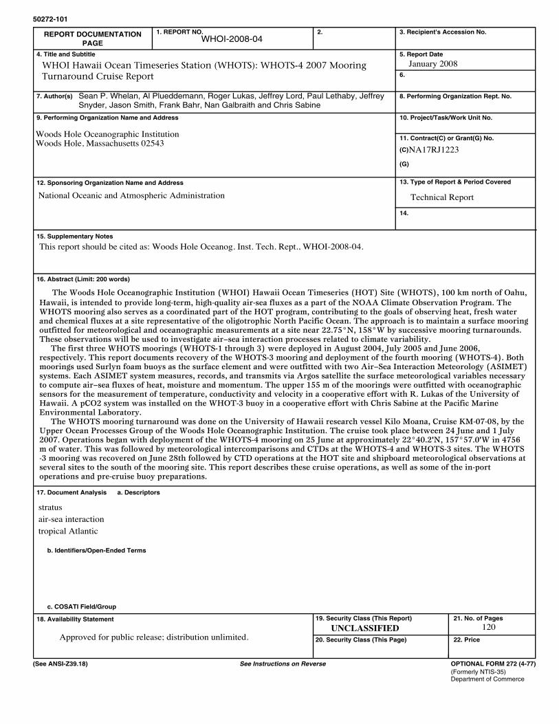
1. REPORT NO.

4. Title and Subtitle

7. Author(s)

9. Performing Organization Name and Address

12. Sponsoring Organization Name and Address

15. Supplementary Notes

16. Abstract (Limit: 200 words)

17. Document Analysis a. Descriptors

b. Identifiers/Open-Ended Terms

c. COSATI Field/Group

18. Availability Statement

REPORT DOCUMENTATION

PAGE

2. 3. Recipient's Accession No.

5. Report Date

6.

8. Performing Organization Rept. No.

10. Project/Task/Work Unit No.

11. Contract(C) or Grant(G) No.

(C)

(G)

13. Type of Report & Period Covered

14.

50272-101

19. Security Class (This Report)

20. Security Class (This Page)

21. No. of Pages

22. Price

OPTIONAL FORM 272 (4-77)

(Formerly NTIS-35)Department of Commerce

(See ANSI-Z39.18) See Instructions on Reverse

UNCLASSIFIED

WHOI Hawaii Ocean Timeseries Station (WHOTS): WHOTS-4 2007 Mooring Turnaround Cruise Report

January 2008

Woods Hole Oceanographic InstitutionWoods Hole, Massachusetts 02543

NA17RJ1223

Technical ReportNational Oceanic and Atmospheric Administration

The Woods Hole Oceanographic Institution (WHOI) Hawaii Ocean Timeseries (HOT) Site (WHOTS), 100 km north of Oahu,Hawaii, is intended to provide long-term, high-quality air-sea fluxes as a part of the NOAA Climate Observation Program. The WHOTS mooring also serves as a coordinated part of the HOT program, contributing to the goals of observing heat, fresh water and chemical fluxes at a site representative of the oligotrophic North Pacific Ocean. The approach is to maintain a surface mooringoutfitted for meteorological and oceanographic measurements at a site near 22.75°N, 158°W by successive mooring turnarounds.These observations will be used to investigate air–sea interaction processes related to climate variability. The first three WHOTS moorings (WHOTS-1 through 3) were deployed in August 2004, July 2005 and June 2006, respectively. This report documents recovery of the WHOTS-3 mooring and deployment of the fourth mooring (WHOTS-4). Bothmoorings used Surlyn foam buoys as the surface element and were outfitted with two Air–Sea Interaction Meteorology (ASIMET)systems. Each ASIMET system measures, records, and transmits via Argos satellite the surface meteorological variables necessaryto compute air–sea fluxes of heat, moisture and momentum. The upper 155 m of the moorings were outfitted with oceanographic sensors for the measurement of temperature, conductivity and velocity in a cooperative effort with R. Lukas of the University of Hawaii. A pCO2 system was installed on the WHOT-3 buoy in a cooperative effort with Chris Sabine at the Pacific Marine Environmental Laboratory. The WHOTS mooring turnaround was done on the University of Hawaii research vessel Kilo Moana, Cruise KM-07-08, by theUpper Ocean Processes Group of the Woods Hole Oceanographic Institution. The cruise took place between 24 June and 1 July 2007. Operations began with deployment of the WHOTS-4 mooring on 25 June at approximately 22°40.2'N, 157°57.0'W in 4756m of water. This was followed by meteorological intercomparisons and CTDs at the WHOTS-4 and WHOTS-3 sites. The WHOTS-3 mooring was recovered on June 28th followed by CTD operations at the HOT site and shipboard meteorological observations atseveral sites to the south of the mooring site. This report describes these cruise operations, as well as some of the in-port operations and pre-cruise buoy preparations.

stratusair-sea interactiontropical Atlantic

120Approved for public release; distribution unlimited.

This report should be cited as: Woods Hole Oceanog. Inst. Tech. Rept., WHOI-2008-04.

WHOI-2008-04

Sean P. Whelan, Al Plueddemann, Roger Lukas, Jeffrey Lord, Paul Lethaby, Jeffrey

Snyder, Jason Smith, Frank Bahr, Nan Galbraith and Chris Sabine