Windlab Limited – LIDAR for Wind Forecasts Project End of Project Report

Lead organisation: Project commencement date: Completion date: Date published: Contact Name: Title: Email: Website:

Windlab Limited 03.Apr.201930.Oct.202005.Mar.2021Keith AyotteChief Scientistkeith.ayotte@windlab.com www.windlab.com

This project received funding from the Australian Renewable Energy Agency (ARENA) as part of ARENA’s Advancing Renewables Program.

1

Project Summary ...................................................................................................................... 2

Project Rationale .................................................................................................................. 2

The Setting and Measurements Taken ................................................................................ 3

Methodology ........................................................................................................................ 4

Outcomes ............................................................................................................................. 4

Project Performance Against Outcomes .................................................................................. 5

Overview of Forecast Model Performance .............................................................................. 7

Qualitative Description of Forecast Methodology ................................................................... 8

Technology and Products Insights ............................................................................................ 9

Transferability of Achievements .............................................................................................. 9

Benefits to Grid, Markets and Consumers ............................................................................. 10

Overview of Financial Benefits ............................................................................................... 10

Areas for Future Improvement .............................................................................................. 10

Key Lessons Learned .............................................................................................................. 10

Seasonality in Wind Data ................................................................................................................. 10

Randomness in Wind Data ................................................................................................. 11

2

Project Summary

Project Rationale

Looking upstream in the wind for information about what the future holds is a common practice. For example, weather forecasts are based in large part on what lies upstream. As weather systems travel from west to east in Australia the conditions associated with the weather systems tend to stay somewhat constant and travel with the system. At the risk of over-simplifying, we often look at the current conditions to our west to see what the weather will be tomorrow or the next day. Here we are talking about time scales or many hours to a few days. In this example we are making use of observations that lie far upstream and lengths of time of up to a few days. However, the principle holds at much smaller scales as well.

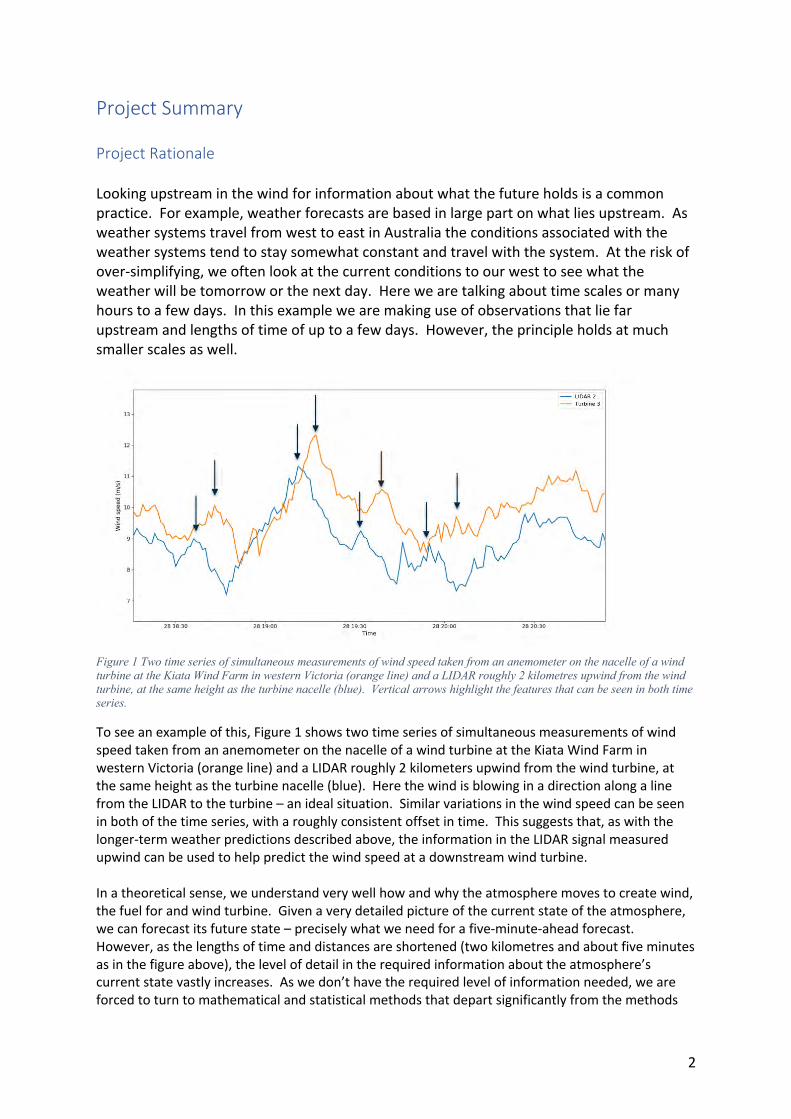
Figure 1 Two time series of simultaneous measurements of wind speed taken from an anemometer on the nacelle of a wind turbine at the Kiata Wind Farm in western Victoria (orange line) and a LIDAR roughly 2 kilometres upwind from the wind turbine, at the same height as the turbine nacelle (blue). Vertical arrows highlight the features that can be seen in both time series.

To see an example of this, Figure 1 shows two time series of simultaneous measurements of wind speed taken from an anemometer on the nacelle of a wind turbine at the Kiata Wind Farm in western Victoria (orange line) and a LIDAR roughly 2 kilometers upwind from the wind turbine, at the same height as the turbine nacelle (blue). Here the wind is blowing in a direction along a line from the LIDAR to the turbine – an ideal situation. Similar variations in the wind speed can be seen in both of the time series, with a roughly consistent offset in time. This suggests that, as with the longer-term weather predictions described above, the information in the LIDAR signal measured upwind can be used to help predict the wind speed at a downstream wind turbine.

In a theoretical sense, we understand very well how and why the atmosphere moves to create wind, the fuel for and wind turbine. Given a very detailed picture of the current state of the atmosphere, we can forecast its future state – precisely what we need for a five-minute-ahead forecast. However, as the lengths of time and distances are shortened (two kilometres and about five minutes as in the figure above), the level of detail in the required information about the atmosphere’s current state vastly increases. As we don’t have the required level of information needed, we are forced to turn to mathematical and statistical methods that depart significantly from the methods

3

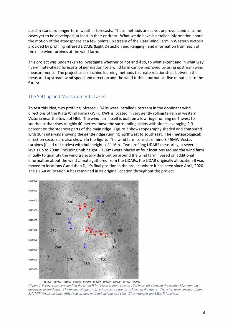
used in standard longer-term weather forecasts. These methods are as yet unproven, and in some cases yet to be developed, at least in their entirety. What we do have is detailed information about the motion of the atmosphere at a few points up stream of the Kiata Wind Farm in Western Victoria provided by profiling infrared LIDARs (Light Detection and Ranging), and information from each of the nine wind turbines at the wind farm. This project was undertaken to investigate whether or not and if so, to what extent and in what way, five-minute-ahead forecasts of generation for a wind farm can be improved by using upstream wind measurements. The project uses machine learning methods to create relationships between the measured upstream wind speed and direction and the wind turbine outputs at five minutes into the future. The Setting and Measurements Taken To test this idea, two profiling infrared LIDARs were installed upstream in the dominant wind directions of the Kiata Wind Farm (KWF). KWF is located in very gently rolling terrain in western Victoria near the town of Nhil. The wind farm itself is built on a low ridge running northwest to southeast that rises roughly 40 metres above the surrounding plains with slopes averaging 2-3 percent on the steepest parts of the main ridge. Figure 2 shows topography shaded and contoured with 10m intervals showing the gentle ridge running northwest to southeast. The (meteorological) direction sectors are also shown in the figure. The wind farm consists of nine 3.45MW Vestas turbines (filled red circles) with hub heights of 116m. Two profiling LIDARS measuring at several levels up to 200m (including hub height – 116m) were placed at four locations around the wind farm initially to quantify the wind trajectory distribution around the wind farm. Based on additional information about the wind climate gathered from the LIDARs, the LIDAR originally at location B was moved to locations C and then D, it’s final position in the project where it has been since April, 2020. The LIDAR at location A has remained in its original location throughout the project.

Figure 2 Topography surrounding the Kiata Wind Farm contoured with 10m intervals showing the gentle ridge running northwest to southeast. The (meteorological) direction sectors are also shown in the figure. The wind farm consists of nine 3.45MW Vestas turbines (filled red circles) with hub heights of 116m. Blue triangles are LIDAR locations.

4

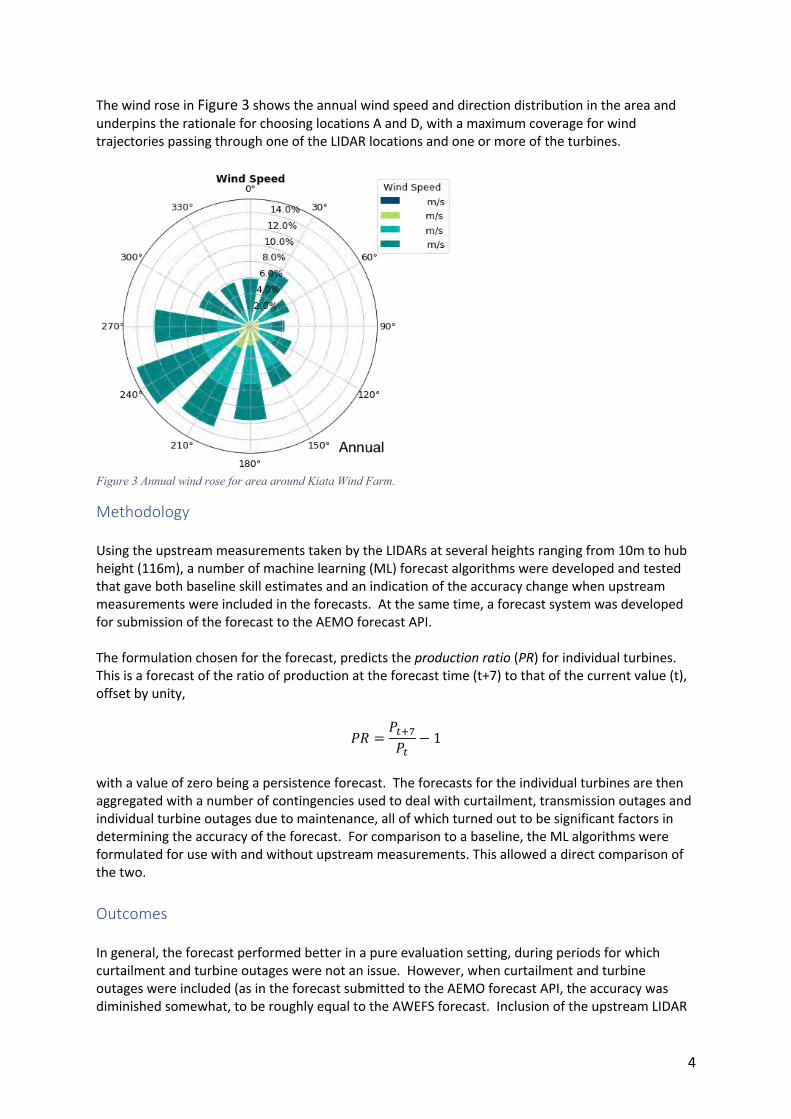
The wind rose in Figure 3 shows the annual wind speed and direction distribution in the area and underpins the rationale for choosing locations A and D, with a maximum coverage for wind trajectories passing through one of the LIDAR locations and one or more of the turbines.

Figure 3 Annual wind rose for area around Kiata Wind Farm.

Methodology Using the upstream measurements taken by the LIDARs at several heights ranging from 10m to hub height (116m), a number of machine learning (ML) forecast algorithms were developed and tested that gave both baseline skill estimates and an indication of the accuracy change when upstream measurements were included in the forecasts. At the same time, a forecast system was developed for submission of the forecast to the AEMO forecast API. The formulation chosen for the forecast, predicts the production ratio (PR) for individual turbines. This is a forecast of the ratio of production at the forecast time (t+7) to that of the current value (t), offset by unity,

𝑃𝑅 =𝑃$%&𝑃$

− 1

with a value of zero being a persistence forecast. The forecasts for the individual turbines are then aggregated with a number of contingencies used to deal with curtailment, transmission outages and individual turbine outages due to maintenance, all of which turned out to be significant factors in determining the accuracy of the forecast. For comparison to a baseline, the ML algorithms were formulated for use with and without upstream measurements. This allowed a direct comparison of the two. Outcomes In general, the forecast performed better in a pure evaluation setting, during periods for which curtailment and turbine outages were not an issue. However, when curtailment and turbine outages were included (as in the forecast submitted to the AEMO forecast API, the accuracy was diminished somewhat, to be roughly equal to the AWEFS forecast. Inclusion of the upstream LIDAR

5

measurements diminished the RMS error by only a few percent. As expected, forecast accuracy was better with two LIDARs included, but inclusion of the second LIDAR contributed an improvement of only one quarter to one third of the first LIDAR. The effectiveness of the method hinges on the amount of time for which the wind was blowing along a line between one of the LIDARs and a turbine. Additionally, the wind speed needs to be such that a parcel of air in the flow will travel a distance equal to that between the upstream measurement location and the turbine. Careful analysis across all of the turbines showed that this ideal situation existed only 3-6 percent of the time if both LIDARs were included and more like 2-4 percent if only one of the LIDARs was included. This is consistent with the forecast error levels found when including one or both of the LIDARs in the ML algorithm. However, it also suggests that if enough upstream measurements can be included, gains in accuracy greater than those found with only two measurements could be achieved. It was also found in evaluations outside the forecast system (so as to limit the effects of curtailments and turbine outages) that though using measurements from lower levels diminished the effectiveness of including upstream measurements, it did so less than expected. This in turn suggested that using more, inexpensive short tower wind measurements could lead to a cost-effective implementation of the methodology. A number of aspects regarding how the seasonality of the wind climate affected training of the ML algorithm and how the general level of entropy (randomness) in the wind measurements affected the forecast accuracy, are covered elsewhere in this report.

Project Performance Against Outcomes This project was very experimental in its nature. The anticipated follow-on from the work would have been a forecasting tool/product based on the methodology. Though it was found that inclusion of upstream wind measurements increased forecast performance, in the final stages of the project it was determined that the increase in accuracy of the forecasts were not sufficient to warrant further development of a forecast system based on the methodology.

Consistent with the exploratory nature of the project, in the original project proposal a number of questions were posed that underpinned the methodology and process of using upstream measurements to improve five-minute-ahead forecasts. These questions were posed to be general in nature so they might apply to anyone else that might have the opportunity to undertake a similar scheme. What follows are the questions and the answers/conclusions that have been derived in undertaking the project.

What is the optimum distance and direction upstream to place wind measurements?

Under ideal conditions to take full advantage of upstream measurements, the wind would be blowing parallel to a line between the measurement location and a turbine. Additionally, the wind would be blowing at a speed that would have a parcel of air leaving the measurement location and arriving at the turbine in exactly the time for which a forecast is being made. In reality this is seldom the case. The wind speed and direction vary in space and time, the parcel trajectories are seldom straight lines and they vary quite markedly over a large range of time scales. This means that conditions are seldom ideal even for one turbine, much less for nine turbines spread across a landscape. Analysis using parcel trajectory probability distributions around the KWF and other trajectory studies show what fraction of the time the conditions are close to ideal as described above and how this is affected by the geographic layout of the wind farm and the measurement

6

locations. The analysis also shows how this ideal fraction varies with time of year. In general, it can be expected that the conditions will be ideal between 3 and 6 percent of the time leading to decreases in RMSE of the raw forecast of just under 2 percent when using one upstream measurement location and just over 2 percent when two upstream measurement locations are used. The analysis shows that the effectiveness of adding upstream measurement locations reduces with each additional location.

How many measurements need to be used to represent the direction variability of the wind?

The economics of taking upstream measurements is dominated by the equipment cost. Achieving significant error reduction with only a few measurements would be ideal. Analysis found that, much as expected, significant seasonal variability in wind speed and direction lead to a more difficult task of making use of the upstream measurements. The wind climate at the Kiata wind farm is dominated by winds form the south and south-western quarters. This or a similarly clustered directional distribution could be expected at many inland locations in Australia. The analysis suggests that, again as could be expected, the decrease in error diminishes with increasing numbers of upstream measurements and is likely quite sensitive to the layout of the wind farm. In this instance the two measurements were upstream (in the prevailing wind direction) from two clusters of turbines making up the wind farm. For larger wind farms (Kiata has only 9 turbines) this might be the factor determining how many measurements are needed – one per cluster of turbines per dominant wind direction. Clearly, for a larger wind farm this could be an uneconomically large number. For a wind farm such as Kiata, the number is more likely to be 3 or 4 which would likely result in decreases in forecast RMSE of 3 to 4 per cent when compared to a similar forecast algorithm without the inclusion of the upstream measurements.

What height should upstream wind measurements be taken?

Using single-direction single-turbine forecast models, it was shown that under ideal circumstances the efficacy of upstream measurements made from much lower (10-20m) heights remained disproportionately high – particularly compared to the significantly reduced costs of the lower measurements. This suggests that if inexpensive low tower measurements can be made, their effectiveness would be disproportionately large relative to the cost reduction over much taller masts. Two factors have shown to affect this outcome. The first is that lower measurements appear to be more sensitive to upstream location in terms of direction and distance from any turbine or cluster of turbines. The second is that significant vegetation such as forest canopies that are of a similar height to the measurement height have a non-negligible effect on the usefulness of the upstream measurements.

Which machine learning algorithms will respond best to the added measurements?

A large number of machine learning algorithms have been experimented with in this project. In the end we settled on a simple artificial neural network forecasting the production ratio. At the core of the forecast system is the machine learning algorithm that forecasts individual turbine output at t+7 minutes. This formulation forecasts the production ratio (PR) for individual turbines - the ratio of production at the forecast time (t+7) to that of the current value (t), offset by unity,

𝑃𝑅 =𝑃$%&𝑃$

− 1

with a value of zero being a persistence forecast. Though using this model does not provide significant accuracy advantages in comparison to other models, it does yield a number of diagnostic

7

parameters that make the model results easier to understand and assess. For example, using this algorithm means that any outliers in the prediction can be more easily detected and it also allows statistical testing of the training to ensure zero production-ratio )*+,-

*+− 1. is not overrepresented.

What increases in accuracy can be expected using upstream measurements?

For the Kiata Wind Farm it appears that with 3 or 4 upstream measurements, the RMSE reduction can be expected to be on the order of 3 to 4 per cent over having no upstream measurements. This is given the current machine learning algorithm and a small wind farm such as Kiata. For larger wind farms with more varied climate the number of measurements to attain that level of increased accuracy would certainly be much greater – and therefore proportionally more expensive.

Though containing a large amount of uncertainty, the economic analysis developed for the project suggests that this level of error reduction is unlikely to be sufficient to justify the additional cost of making the upstream measurements.

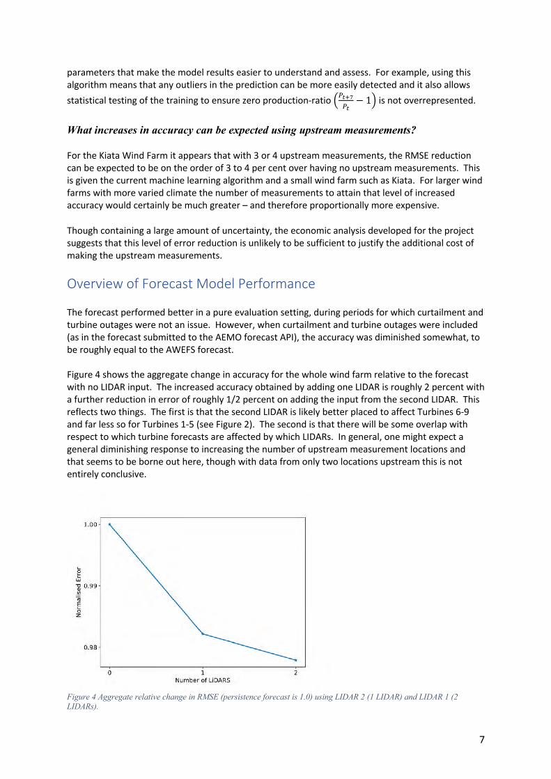
Overview of Forecast Model Performance The forecast performed better in a pure evaluation setting, during periods for which curtailment and turbine outages were not an issue. However, when curtailment and turbine outages were included (as in the forecast submitted to the AEMO forecast API), the accuracy was diminished somewhat, to be roughly equal to the AWEFS forecast. Figure 4 shows the aggregate change in accuracy for the whole wind farm relative to the forecast with no LIDAR input. The increased accuracy obtained by adding one LIDAR is roughly 2 percent with a further reduction in error of roughly 1/2 percent on adding the input from the second LIDAR. This reflects two things. The first is that the second LIDAR is likely better placed to affect Turbines 6-9 and far less so for Turbines 1-5 (see Figure 2). The second is that there will be some overlap with respect to which turbine forecasts are affected by which LIDARs. In general, one might expect a general diminishing response to increasing the number of upstream measurement locations and that seems to be borne out here, though with data from only two locations upstream this is not entirely conclusive.

Figure 4 Aggregate relative change in RMSE (persistence forecast is 1.0) using LIDAR 2 (1 LIDAR) and LIDAR 1 (2 LIDARs).

8

Qualitative Description of Forecast Methodology At the core of the forecast system is the machine learning algorithm that forecasts individual turbine output at t+7 minutes. Many forecast algorithms could have been used and Windlab has experimented with a large number of them. Though we are still working on improving the core algorithm, the current formulation forecasts the production ratio (PR) for individual turbines. This is a forecast of the ratio of production at the forecast time (t+7) to that of the current value (t), offset by unity,

𝑃𝑅 =𝑃$%&𝑃$

− 1

with a value of zero being a persistence forecast. Though using this model does not provide significant accuracy advantages in comparison to other models, it does yield a number of diagnostic parameters that make the model results easier to understand and assess. For example, using this algorithm means that any outliers in the prediction can be more easily detected and it also allows statistical testing of the training to ensure zero production-ratio )*+,-

*+− 1. is not overrepresented.

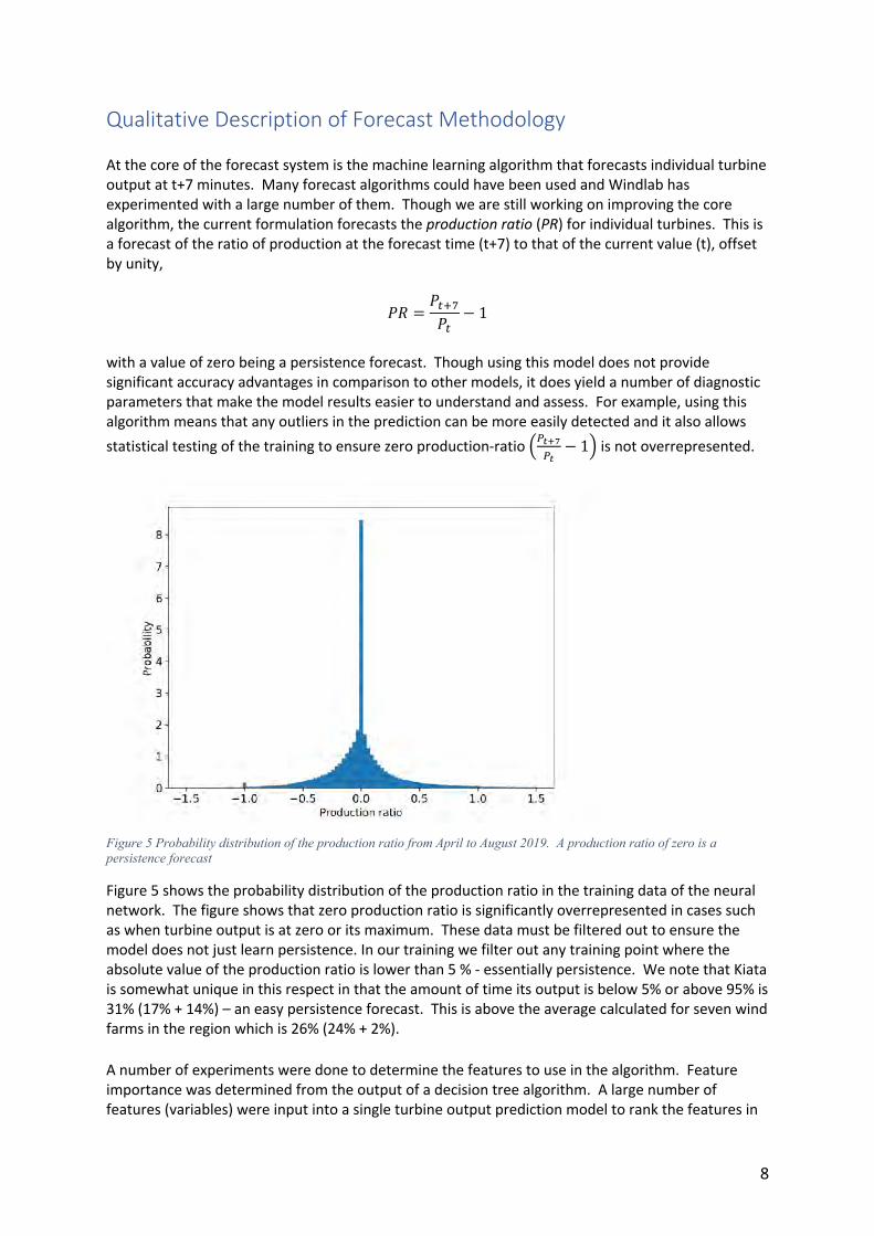
Figure 5 Probability distribution of the production ratio from April to August 2019. A production ratio of zero is a persistence forecast

Figure 5 shows the probability distribution of the production ratio in the training data of the neural network. The figure shows that zero production ratio is significantly overrepresented in cases such as when turbine output is at zero or its maximum. These data must be filtered out to ensure the model does not just learn persistence. In our training we filter out any training point where the absolute value of the production ratio is lower than 5 % - essentially persistence. We note that Kiata is somewhat unique in this respect in that the amount of time its output is below 5% or above 95% is 31% (17% + 14%) – an easy persistence forecast. This is above the average calculated for seven wind farms in the region which is 26% (24% + 2%). A number of experiments were done to determine the features to use in the algorithm. Feature importance was determined from the output of a decision tree algorithm. A large number of features (variables) were input into a single turbine output prediction model to rank the features in

9

importance. Not unexpectedly the largest feature importance, by more than a factor of two over the next largest feature, was the average wind speed. This was followed by wind direction relative to nacelle centerline and wind speed standard deviation. The remaining features diminished significantly in importance relative to those mentioned above. Based on this information and other investigations, the following features were chosen,

𝑃$%&𝑃$

− 1 = 𝑓(𝑢, 𝑣, 𝑉56$7, 𝐷𝑖𝑟;<=)

where u and v were the components of the full wind vector and provide some directional information to the machine learning fit. In this and efforts to understand and recreate a turbine power curve, it was found that the angle of the wind to the nacelle centerline was important. This is due largely to effect of the reduced cross-sectional area of the turbine disk with the flow approaching at an angle. Similarly, the standard deviation of the wind speed, an indication of turbulence levels in the flow impinging on the turbine blades, was also a strong feature. After numerous experiments on a fully connected network with one hidden layer, analysis of autocorrelation showed that the autocorrelation of turbine output of more than 6-7 steps is statistically not significant leading to the inclusion of 10 historic values in the model.

Technology and Products Insights

The LIDARs used in the project were ZephIR ZX300 powered by stand-alone power supplies supplied by Energy3 (www.energy3.co.nz). Both the LIDARs and the power supplies performed very well with both suppliers (ZephIR and Energy3) providing good support. The only hardware failure was a modem in one of the power supplies which was replaced promptly with minimal loss of data.

The main software tool used in building and training the ML algorithms for the forecast was TensorFlow from Google. We also used XGBoost for feature sensitivity studies. Both of these tools were very useful and performed well. Both were implemented on a desktop computer with 2x Nvidia RTX 2080 TI 11GB OC graphics cards, each of which had 4352 CUDA Cores for distributed processing of TensorFlow tasks. This significantly reduced model training times.

Transferability of Achievements

As noted above, the project was experimental in nature with some prospect for development of a forecasting methodology if it was found that upstream measurements provided significant forecast improvement. In the design of the project it was intended that a body of knowledge would be generated around the following questions:

- What is the optimum distance and direction upstream to place wind measurements? - How many measurements need to be used to represent the direction variability of the wind? - What height should upstream wind measurements be taken? - Which machine learning algorithms will respond best to the added measurements? - What increases in accuracy can be expected using upstream measurements?

The knowledge included in the responses to these questions (see above) and in other reports provided to ARENA is generally applicable to work undertaken by others of a similar nature.

10

Benefits to Grid, Markets and Consumers As the project did not result in significant gains in forecast accuracy, no commercial undertaking followed from the project. As such the grid, markets and consumers did not receive any benefits.

Overview of Financial Benefits See above.

Areas for Future Improvement As noted above and in reports provided to ARENA, it appears that forecast accuracy might be improved by the application of an increased number (possibly as many as 8-10) of less expensive tower-based measurements. If instrumented meteorological towers with communications can be provided for less than, say, $10K each, there is some scope for improving the forecast accuracy by several percent. However, the financial model built for the project has more uncertainty than would be necessary to determine if even a 10 percent improvement would be sufficient to base a commercial forecasting undertaking on.

Key Lessons Learned In addition to answering the five technical/scientific questions presented above, during the development of the forecast, a number of physical (meteorological) and statistical issues were identified that affected the forecast accuracy. Seasonality in Wind Data Figure 3 above shows an annual wind rose measured from one of the LIDARs on site. Though the annual wind rose suggests a constant flow from the south and southwest sectors, it hides significant monthly variation.

Figure 6 Monthly wind roses for the March, May and June,2020. The wind roses show the significant variation in wind speed and direction through the seasons of the year

Figure 6 shows the wind roses for the months of March, May and June 2020. These (and other months) are not well represented by the annual average wind rose. The variation across the months reflects the seasonality in the wind climate. This indicates that the statistics of the wind climate are not stationary on an annual basis. Experiments with training models on short periods of data, for

11

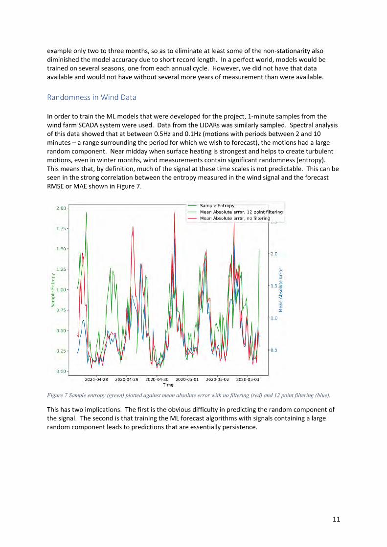
example only two to three months, so as to eliminate at least some of the non-stationarity also diminished the model accuracy due to short record length. In a perfect world, models would be trained on several seasons, one from each annual cycle. However, we did not have that data available and would not have without several more years of measurement than were available. Randomness in Wind Data In order to train the ML models that were developed for the project, 1-minute samples from the wind farm SCADA system were used. Data from the LIDARs was similarly sampled. Spectral analysis of this data showed that at between 0.5Hz and 0.1Hz (motions with periods between 2 and 10 minutes – a range surrounding the period for which we wish to forecast), the motions had a large random component. Near midday when surface heating is strongest and helps to create turbulent motions, even in winter months, wind measurements contain significant randomness (entropy). This means that, by definition, much of the signal at these time scales is not predictable. This can be seen in the strong correlation between the entropy measured in the wind signal and the forecast RMSE or MAE shown in Figure 7.

Figure 7 Sample entropy (green) plotted against mean absolute error with no filtering (red) and 12 point filtering (blue).

This has two implications. The first is the obvious difficulty in predicting the random component of the signal. The second is that training the ML forecast algorithms with signals containing a large random component leads to predictions that are essentially persistence.

12

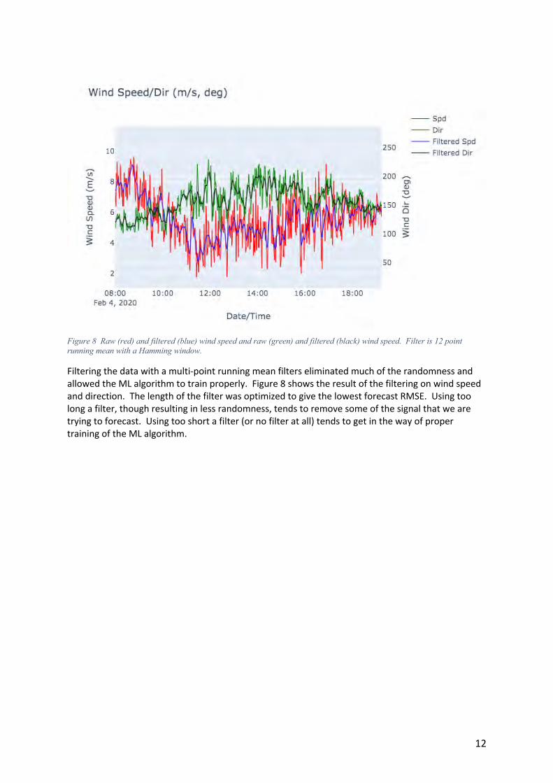
Figure 8 Raw (red) and filtered (blue) wind speed and raw (green) and filtered (black) wind speed. Filter is 12 point running mean with a Hamming window.

Filtering the data with a multi-point running mean filters eliminated much of the randomness and allowed the ML algorithm to train properly. Figure 8 shows the result of the filtering on wind speed and direction. The length of the filter was optimized to give the lowest forecast RMSE. Using too long a filter, though resulting in less randomness, tends to remove some of the signal that we are trying to forecast. Using too short a filter (or no filter at all) tends to get in the way of proper training of the ML algorithm.