project report shenandoah 1.0m nps lidar lidar survey

Northrop Grumman Page | 1

Project Report

Shenandoah 1.0m NPS LiDAR LiDAR Survey

PREPARED FOR: UNITED STATES GEOLOGICAL SURVEY

& UNITED STATES ARMY CORPS OF ENGINEERS ENGINEER RESEARCH AND DEVELOPMENT CENTER

PREPARED BY:

NORTHROP GRUMMAN CORPORATION

________________________________________ 2011 SHENANDOAH 1.0M NPS LIDAR

CONTRACT # G10PC00150 to #02

NGC INTERNAL #B1M958021

DATE: 01 JUNE 2011


Project Summary

This report documents the performance of GPS ground control surveys, airborne acquisition, and subsequent calibration and production processing of Light Detection and Ranging (LiDAR) data for the Shenandoah 1.0m NPS LiDAR project. The entire survey area for northern Shenandoah valley encompasses 714 square miles. The Shenandoah LiDAR project, ordered by the USGS, provides precise elevations acquired by the Optech 3100 serial number 07SEN203 airborne LiDAR sensor. The LiDAR point cloud was acquired at a nominal point spacing of 1.0 meter. High accuracy multiple return LiDAR data, both raw and separated into several classes, are provided, along with hydro flattening breaklines and bare earth DEM tiles. The classified point cloud and bare earth DEM data has been tiled into 1500 meter by 1500 meter tiles, stored in LAS format version 1.2 (point format 1), and LiDAR returns coded into 6 separate ASPRS classes. The LiDAR data and derivative products produced are in compliance with the U.S. Geological Survey National Geospatial Program Guidelines and Base Specifications, Version 13-ILMF 2010. The LiDAR data were acquired by Northrop Grumman, 3001 Operating Unit (OU), which were flown over nine missions between March 01, 2011 and March 09, 2011. The Northrop Grumman 3001 OU implemented a variety of quality assurance and quality control procedures throughout the processing phases in order to provide a product that meets or exceeds the requirements specified in the USGS contract G10PD02496.

This LiDAR data set has met vertical accuracy requirements and has been validated to be an accurate representation of the ground at the time of survey.


Table of Contents ____________________________________________________________________________________

Project Summary .........................................................................................................................................2

Table of Contents .........................................................................................................................................3

1 Collection Report ...................................................................................................................................5

1.1 Mission Planning and Acquisition ..........................................................................................5

1.2 Flight Parameters ..................................................................................................................6

1.3 Dates Flown ...........................................................................................................................6

1.4 GPS Collection Parameters ....................................................................................................6

1.5 Projection / Datum ................................................................................................................6

1.6 Base Stations Used ................................................................................................................7

1.7 Flight Logs ..............................................................................................................................7

2 Processing Report .................................................................................................................................8

2.1 Airborne Survey Processing ...................................................................................................8

2.2 Swath LAS File Naming Scheme .............................................................................................8

2.3 Flight Line Calibration ............................................................................................................9

2.4 Point Classification ..............................................................................................................11

2.4 Methodology for Breakline Collection and Hydro-flattening ..............................................11

2.5 Product generation - Raw point cloud data, LAS format .....................................................12

2.6 Product generation - Classified point cloud tiles, LAS format .............................................12

2.7 Product generation - Bare earth DEM tiles .........................................................................13

2.8 Product generation - Breaklines, ESRI Shapefile format ....................................................13

2.9 Product generation - Digital spatial representation of precise extents of Raw Point Cloud data, ESRI Shapefile format ...............................................................................................13

3 QA/QC Report .....................................................................................................................................14

3.1 Post Data Collection QC ......................................................................................................14

3.2 Data Calibration QC ............................................................................................................14

3.3 Horizontal Accuracy QC ......................................................................................................15


3.4 Classified Point Cloud Tiles QC ..........................................................................................15

3.5 Bare Earth DEM QC ...........................................................................................................18

3.6 Breakline QC ......................................................................................................................19

3.7 Swath Extent QC ................................................................................................................19

3.8 Metadata QC .....................................................................................................................19

4 Conclusion ...........................................................................................................................................20


COLLECTION REPORT

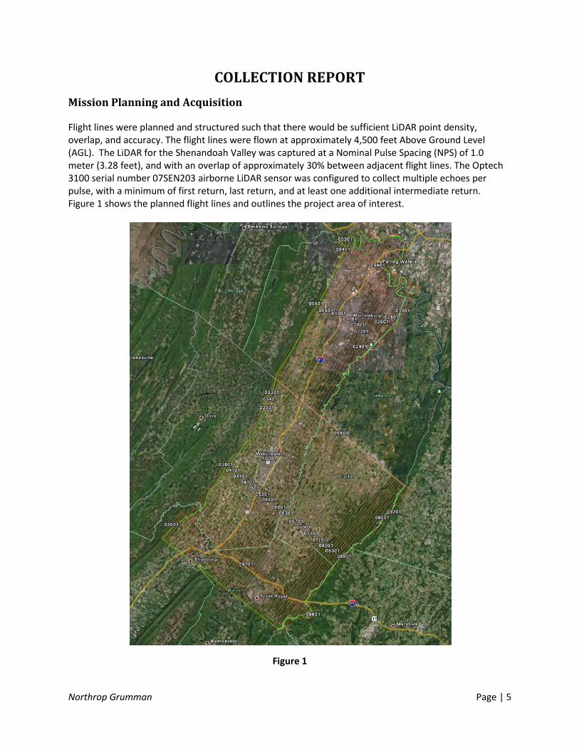
Mission Planning and Acquisition Flight lines were planned and structured such that there would be sufficient LiDAR point density, overlap, and accuracy. The flight lines were flown at approximately 4,500 feet Above Ground Level (AGL). The LiDAR for the Shenandoah Valley was captured at a Nominal Pulse Spacing (NPS) of 1.0 meter (3.28 feet), and with an overlap of approximately 30% between adjacent flight lines. The Optech 3100 serial number 07SEN203 airborne LiDAR sensor was configured to collect multiple echoes per pulse, with a minimum of first return, last return, and at least one additional intermediate return. Figure 1 shows the planned flight lines and outlines the project area of interest.

Figure 1


Flight Parameters Detailed project planning was performed for this project. This planning was based on project specific requirements and the characteristics of the project site. The basis of this planning included the required accuracies, type of development, amount and type of vegetation within the project area, the required data posting, and potential altitude restrictions for flights in the general area. A brief summary of the aerial acquisition parameters for this project are shown in the table below:

These collection parameters resulted in a nominal swath width of 891.32 meters (2924.28 feet) and an average point distribution of 1 point per square meter.

Dates Flown

The Shenandoah Valley LiDAR Project consists of nine missions, which were flown between March 01, 2011 and March 09, 2011.

GPS Collection Parameters Collection parameters for this project included the following:

Projection / Datum

The spatial reference systems used were UTM Zone 17N, NAD83, meters with elevations in NAVD88, meters. Geoid09 was used in the translation of elevations from ellipsoid to orthometric heights.

Parameter Value Flying Height (AGL) 4500 feet Nominal ground speed 125 knots Field of View 36˚ Laser Rate 70 Hz Scan Rate 33 Hz Maximum Cross Track Posting

0.9 meters (2.95 feet)

Maximum Along Track Posting

0.9 meters (2.95 feet)

Nominal Side lap 30%

Parameter Value Maximum PDOP 2.4 Minimum number of SVs 7 Ground collection epoch 2 Hz (1 sec)


Base Stations Used

The Airborne Global Positioning System (ABGPS) used was the Novatel GPS-702 data collection unit, logging at 2 hertz, paired with an Novatel DL-4+L1/L2 antenna, which is a fixed height antenna.

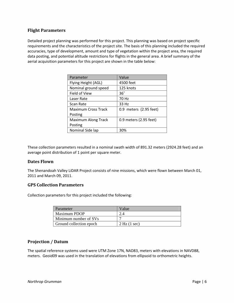
Flight Logs

The LiDAR flight team kept daily logs throughout the survey acquisition, as seen in Figure 2. These flight logs contain various information about that days flying conditions, sensor setup, date, project, lines flown, start and stop times for each line, and any other additional comments and attributes that may be relevant for that particular mission.

Figure 2


PROCESSING REPORT

Airborne Survey Processing

Beginning the LiDAR data processing, the Airborne GPS is extracted and computed to give the best possible positional accuracies. The IMU data is then analyzed and the lever arms corrected to achieve consistent airborne data. Upon the creation of the SBET file, the LAS files are computed using Optech’s proprietary post-processing software. The Quality Assurance (QA) analyst does a thorough review for any quality issues with the data. This could include data voids, high and low points, and data gaps. The data voids or high points could be the result of any high elevation point returns, including clouds, steam from industrial plants, flocks of birds, or any other anomaly. The LiDAR data is reviewed at the flight line level in order to verify sufficient flight line overlap as required to ensure there are no data gaps between usable portions of the swath. Each line is also assessed to fully address the data’s overall accuracy and quality. Within this Quality Assurance/Quality Control (QA/QC) process, four fundamental questions were addressed:

Did the LiDAR system perform to specifications? Did the data have any discrepancies or anomalies? If there were any discrepancies or anomalies, were they addressed accordingly? Was the data complete?

Swath LAS File Naming Scheme

Two distinct file name encoding schemes were developed for the swath LAS files which are compatible with the allowable range of values for the LAS File Source ID (header record) and Point Source ID (point records) fields. These fields are stored within the LAS files as a 2-byte unsigned integer (unsigned short) value, which can range from 0 to 65535. The 5-digits supported by this range were subdivided into two or three groups based on the type of swath the file would contain.

In the case of bore sight (for calibration) and tie line swaths, two groups of digits were used. The grouping consists of first, a three digit flight line number (left padded with zeros if necessary) then, a two digit version number. The flight line number reflects the unique number assigned to the flight path as designated in the project flight plan. Initial acquisition of a planned calibration or tie line is designated as version one. Upon subsequent re-flight or re-acquisition, should such be necessary, the version number is incremented relative to the most recent prior acquisition. For example, a file name of "09715.las" would indicate that the file contains the swath from planned flight line number 97, and is the 15th version (i.e. the line was flown 14 times previously).

In the case of project data swaths, three groups of digits were used. These groups consist of a three digit flight line number (as above), a single digit revision number, and a one digit part number. The initial acquisition of a project data line is designated as revision zero. (It should be noted that this is in contrast to the use of a version number as for the bore sight and tie lines above. The primary reason for this difference is to allow the full numeric range, from 0 to 9, to be used for this single digit value.) For the current project, the part number will have a value of either 1 or 2 due to the requirement to split swath files that were larger than two gigabytes in size. For the current project, no swaths required


splitting into more than two parts. As an example, a file named "04711.las" indicates flight line number 47, revision number 1 (i.e. the line was flown once before), and part number 1.

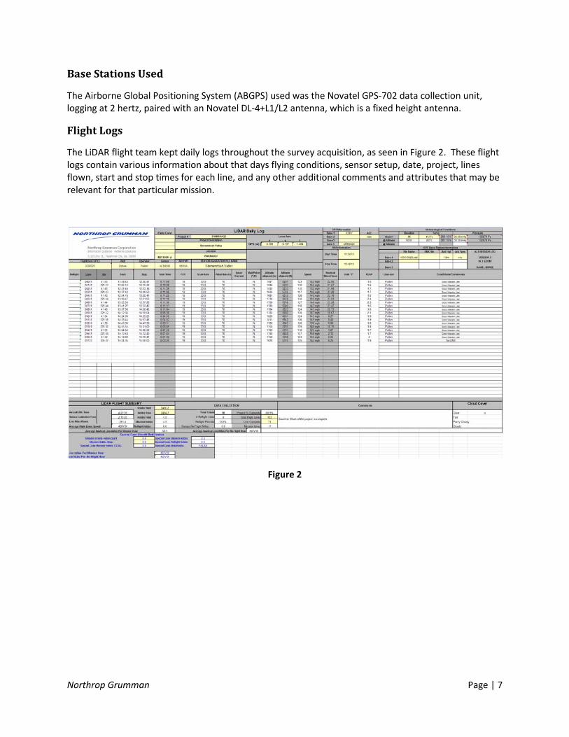
Flight line Calibration

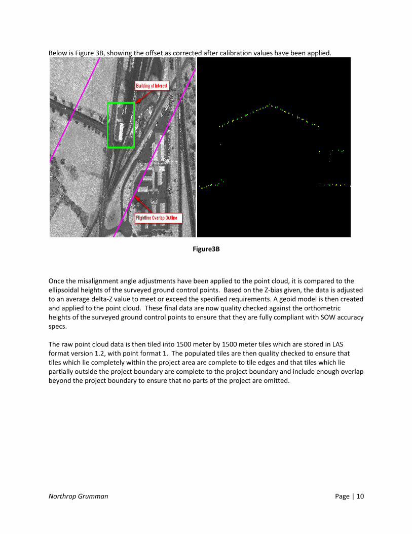
Next, the LiDAR data set is calibrated using suitable test sites identified throughout the project area within the raw point cloud. The sensor misalignment angles (heading, roll, and pitch) and mirror scale are then adjusted based on measurements taken between adjacent flight swaths within the point cloud at the test site locations. The Figures 3A and 3B below demonstrate the pre- and post-calibration data.

Figure 3A, shows a predominantly horizontal offset of 3.23 meter in the overlapping region between two swaths.

Figure 3A


Below is Figure 3B, showing the offset as corrected after calibration values have been applied.

Figure3B

Once the misalignment angle adjustments have been applied to the point cloud, it is compared to the ellipsoidal heights of the surveyed ground control points. Based on the Z-bias given, the data is adjusted to an average delta-Z value to meet or exceed the specified requirements. A geoid model is then created and applied to the point cloud. These final data are now quality checked against the orthometric heights of the surveyed ground control points to ensure that they are fully compliant with SOW accuracy specs. The raw point cloud data is then tiled into 1500 meter by 1500 meter tiles which are stored in LAS format version 1.2, with point format 1. The populated tiles are then quality checked to ensure that tiles which lie completely within the project area are complete to tile edges and that tiles which lie partially outside the project boundary are complete to the project boundary and include enough overlap beyond the project boundary to ensure that no parts of the project are omitted.


Point Classification

After calibration, the data was cut into 1500 meter by 1500 meter tiles, per the Statement of Work. The tiles are contiguous, do not overlap, and are suitable for seamless topographic data mosaics that include no "no data" areas. The names of the tiles include numeric column and row. Ground classification algorithms were then applied. The data was automatically classified into the following classes:

• Class 1 - Processed, but unclassified • Class 2 - Bare Earth Ground • Class 11 - Withheld

o This class includes: outliers, blunders, noise points, geometrically unreliable points near the extreme edge of the swath, and other points deemed unusable that are identified during pre-processing or though the ground classification algorithms

The following classes were also used during the task of point classification Quality Control (QC), manual edits and breakline creation:

• Class 7 - Noise (low or high, manually identified) • Class 9 - Water • Class 10 - Ignored Ground (Breakline Proximity)

Class 7, Noise, was used for points subsequently identified during manual edits and QC. False, extreme high, and extreme low returns were put in this class if found erroneously classified as Ground. Class 10, Ignored Ground, was used for points previously classified as Bare-Earth/Ground, but whose proximity to a subsequently added breakline required that it be excluded during DEM generation. This proximity was 1 meter (3.28 feet).

Each tile was reviewed by an experienced LiDAR analyst to verify the results of the automated ground filters. Points were manually reclassified when necessary. Hydro flattening breaklines were collected, per the project specification, which resulted in the point classifications for Classes 9 (Water) and 10 (Ignored Ground).

Methodology for Breakline Collection and Hydro-flattening

Breaklines were collected manually, based on the LiDAR surface model in TerraModeler version 011. The classification of points as either water or ground was determined based on a combination of factors in the data: point density, voids in data returns, and flatness of the surface. Auxiliary information, such as publically available imagery, as well as ESRI's Hydro layer was used as an additional aid in decision making.

When an area had sufficient voids in returns, i.e. the point density was sparse due to absorption, and the area when viewed in cross-section appeared to be flat with no apparent vegetation growth, then it was determined to be water. There were cases where a significantly sized body of water did have returns on the surface of the water, but based on it being completely flat in cross-section and existing point return voids in close proximity within the bounds of the feature, the area was classified as water.

Along smaller streams and lakes, if there were sufficient point returns that were similar in density to the surrounding ground data, those points were determined to be likely ground returns as well. It was not possible to verify or determine with 100% certainty whether dense point returns within water bodies


were actual ground, or floating plant debris/algae mats on the water surface. If there were sufficiently dense returns, then it was classified as ground.

Inland ponds and lakes were given a single, constant elevation via hydro flattening breaklines. This elevation value was determined by reviewing multiple cross sectional views of the point data at various locations around the feature in order to identify the elevation of point returns on the surface of the water.

Sloped inland stream and river breaklines have a gradient longitudinally and are flat and level, bank-to-bank, perpendicular to the apparent flow centerline. This was accomplished by setting benchmark heights along the breakline feature at each endpoint and at intervals as needed. These heights were determined by viewing cross sections at each benchmark, identifying the elevation. The feature was then sloped using linear interpolation to set the vertex heights between the benchmarks. The sloped feature was then checked at multiple places to verify the fit to the point data. At any given point along the sloped breakline, the water surface should be at or just below the adjacent ground data.

After the manual point classification edits and breakline collection process, the tiles go through a final round of QC by our most experienced analysts. Point classifications, breakline collection, and breakline heights are verified. After all data has passed the final round of QC, the Bare Earth LiDAR products are generated from the classified LAS tiles.

Product Generation - Raw Point Cloud Data, LAS format

Following calibration, all raw swaths are evaluated to ensure that the data meets all deliverable requirements. The point cloud is verified to the extent of the AOI and that all points meet LAS 1.2 requirements. GPS times are set to 'Adjusted GPS Time' to allow each return to have a unique timestamp.

Long swaths resulting in a LAS file larger than 2GB are split into segments no greater than 2GB each, without splitting point “families” (i.e. groups of returns belonging to a single source laser pulse). Each segment is subsequently regarded as a unique swath and is assigned a unique File Source ID and each point given a Point Source ID equal to its File Source ID. Georeference information is added and verified. Intensity values are in native radiometric resolution. All swaths, including cross-ties and calibration sites, are included in this deliverable.

Following calibration and correct naming convention application, the raw point cloud is organized and structured per swath as the first deliverable.

Product Generation - Classified Point Cloud Tiles, LAS format

Following calibration, the data was cut into 1500 meter by 1500 meter tiles, per the Statement of Work, and ground classification algorithms were applied. The data was reviewed by experienced LiDAR analysts, on a tile by tile basis, and ground classifications were manually corrected, as needed. The classified tiles went through one round of quality control and point classification edits, using experienced LiDAR analysts. A second round of QC was performed by our most experienced analysts, which sometimes involved minor edits to the point classifications.

After the point data classifications were verified to meet the standards of the project specification and the U.S. Geological Survey National Geospatial Program LiDAR Guidelines and Base Specification, Version 13 – ILMF 2010, the LAS tiles were clipped to the Area of Interest polygon.


Breakline collection dictated the classification of "Ignored Ground", class 10. Bare earth LiDAR points in close proximity to breaklines were classified to "Ignored Ground", in order to exclude the data from the DEM creation process. The distance threshold used for this reclassification was 1 meter (3.28 feet).

The "Ground" class for all classified point cloud tiles was loaded into TerraScan version 011 to verify completeness of the dataset.

Product Generation - Bare Earth DEM Tiles

After a satisfactory review of the classified point cloud tiles, these tiles were used to create the Bare Earth DEM raster tiles. Using TerraModeler version 011, the classified point cloud tiles and hydro flattened breaklines were combined to create triangulated surface models and exported as lattice files, in ArcInfo ASCII raster format, with a cell size of 1.0 meter. The Digital Elevation Model (DEM) naming convention matches the classified LAS tiling scheme. The ASCII raster files were verified to contain no NODATA pixels, within the Area of Interest.

The ASCII raster files were converted to ERDAS Imagine (IMG) format and then clipped to the Area of Interest polygon. The bare earth IMG tiles are reviewed to ensure that there is a seamless data set, with no edge artifacts or mismatches between tiles. Any areas outside the Area of Interest, but within the tiling scheme, are coded with a unique NODATA value.

Product Generation - Breaklines, ESRI Shapefile format

All breaklines were collected in MicroStation v8 DGN format then combined into a single master DGN file. Breakline collection adheres to the project specification for feature size and hydro flattening requirements. Breaklines were collected alongside the Quality Control and manual point classification of the LiDAR point data while viewing a surface model of a single tile of data.

Inland ponds and lakes were given a single, constant elevation via hydro flattening breaklines. Inland stream and river breaklines were sloped using a proprietary macro, which interpolated the vertex heights between the established benchmark heights.

The master DGN was then converted to ESRI Shapefile format, as 3D polylines. All breaklines used to modify the surface for the purpose of DEM creation are considered a data deliverable.

Product Generation - Digital Spatial Representation of Precise Extents of Raw Point Cloud data, ESRI Shapefile format

Swath extents for each flight line were computed and combined to form one shapefile which contains individual swath polygons per acquired line. Since the mission lines were very large, a thinning method was used to decrease overall file size. The thinning method involved placing a uniform grid with a specified cell size and keeping only one point per grid cell.

The thinned LAS file is triangulated into a Triangulated Irregular Network (TIN) and the boundary extracted using a concave approach. Triangles with edges that exceed 50 meters (164 feet) on the outer regions of the TIN are excluded. The domain of the resulting TIN is calculated and polygons are produced which represent each swath’s extents. This method calculates the actual extents of the LiDAR source data, exclusive of TIN artifacts or raster NODATA areas.


The resulting shapefile presents an accurate representation of each swath without being overly complex. The swath polygons are then dissolved, to form a single polygon for each swath, and combined with the other mission lines in the shapefile format.

QA/QC REPORT

Post Data Collection QC

After extraction of the o-files, no-data regions were analyzed and validated. Each swath underwent a visual QC for void regions within the swath itself, and in the overlapping regions of the adjacent swaths as well. All data voids in question were examined and verified as being the result of water bodies or areas of low reflectivity.

Data Calibration QC

The data posting is a function of flight altitude, airspeed, scan angle, scan rate, laser pulse rates, and terrain relief. The above functions are taken into consideration at the time of flight planning. Data acquisition procedures play a role in the success of this method. Many parameters are considered in order to achieve the maximum possible GPS positioning accuracy, such as the separation between the airborne and base station GPS receivers, satellite geometry as reflected by the Position Dilution of Precision (PDOP), signal multipath, and many other factors. The post-flight data processing software maximizes detection probability while minimizing false alarms. It corrects for several unavoidable, but predictable, biases from the environment as well as removing effects inherent to the hardware configuration. Monitoring the data during collection is only part of the process done to assure proper operation of equipment and ultimately, data quality. However, all subsystems may indicate correct operating parameters (precision), but that does not mean that together they are providing correct solutions (accuracy). In order to validate the collection process, calibration checks are performed. These procedures allow the operator to know if the subsystems have been set up properly and if there are any inherent biases in the instrumentation. Prior to the calibration process, the GPS base stations, which are correlated to NGS CORS network stations, are processed in conjunction with the airborne GPS raw observables to determine the aircraft positions. The processed GPS positions are combined with the inertial data (IMU) using the Applanix POSPacTM software in a closed loop fashion (forward and backward solution with Kalman filter option) to compute the solution parameters, namely position, velocity, and attitude. The resulting SBET file and the LiDAR data are used in the post-processing software as input to compute the calibration parameters.


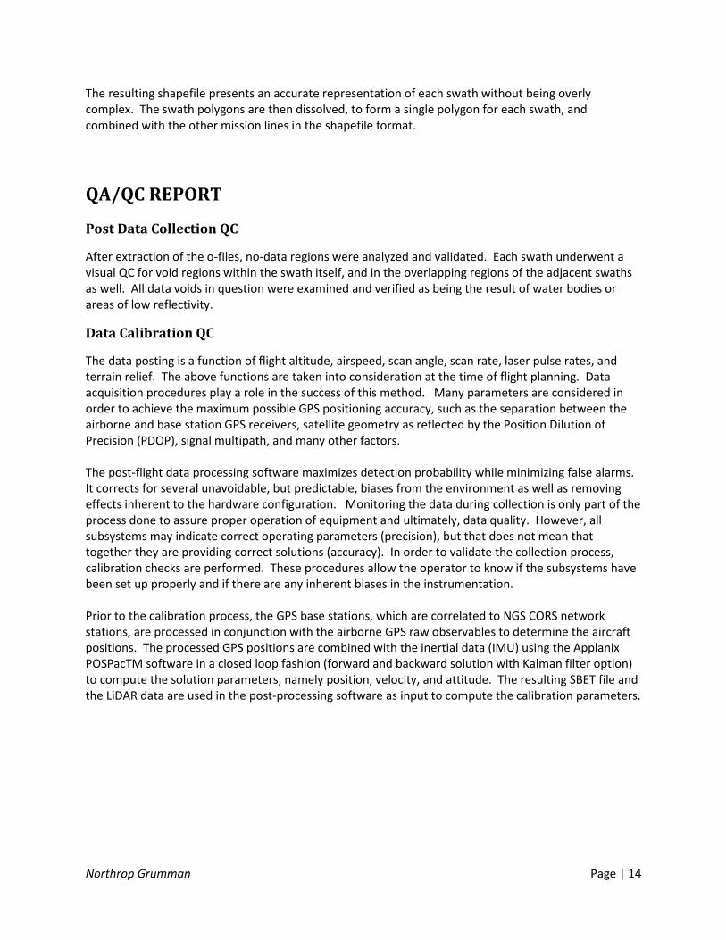
Horizontal Accuracy QC

In figure 4 you will see the horizontal accuracy with lines digitized by a Northrop Grumman analyst between the LiDAR and horizontal check points acquired by the field crew. These sites were randomly spaced throughout the project area.

Figure 4

Classified Point Cloud Tiles QC

The classified point cloud tiles are delivered in fully compliant LAS v1.2 format, with point format 1 and geo-reference information included in the LAS header. GPS times are recorded as Adjusted GPS Time and Intensity values are in native radiometric resolution.

Parameter Value Number of QA/QC Points 6

Minimum difference 0.17 meters Maximum difference 0.59 meters Average difference 0.37 meters


The calibrated data was cut into tiles and then processed using proprietary ground filter macros. The data was reviewed, on a tile by tile basis, and ground classifications were corrected manually, when needed. The point classification scheme is consistent across the entire project and adheres to the project specification.

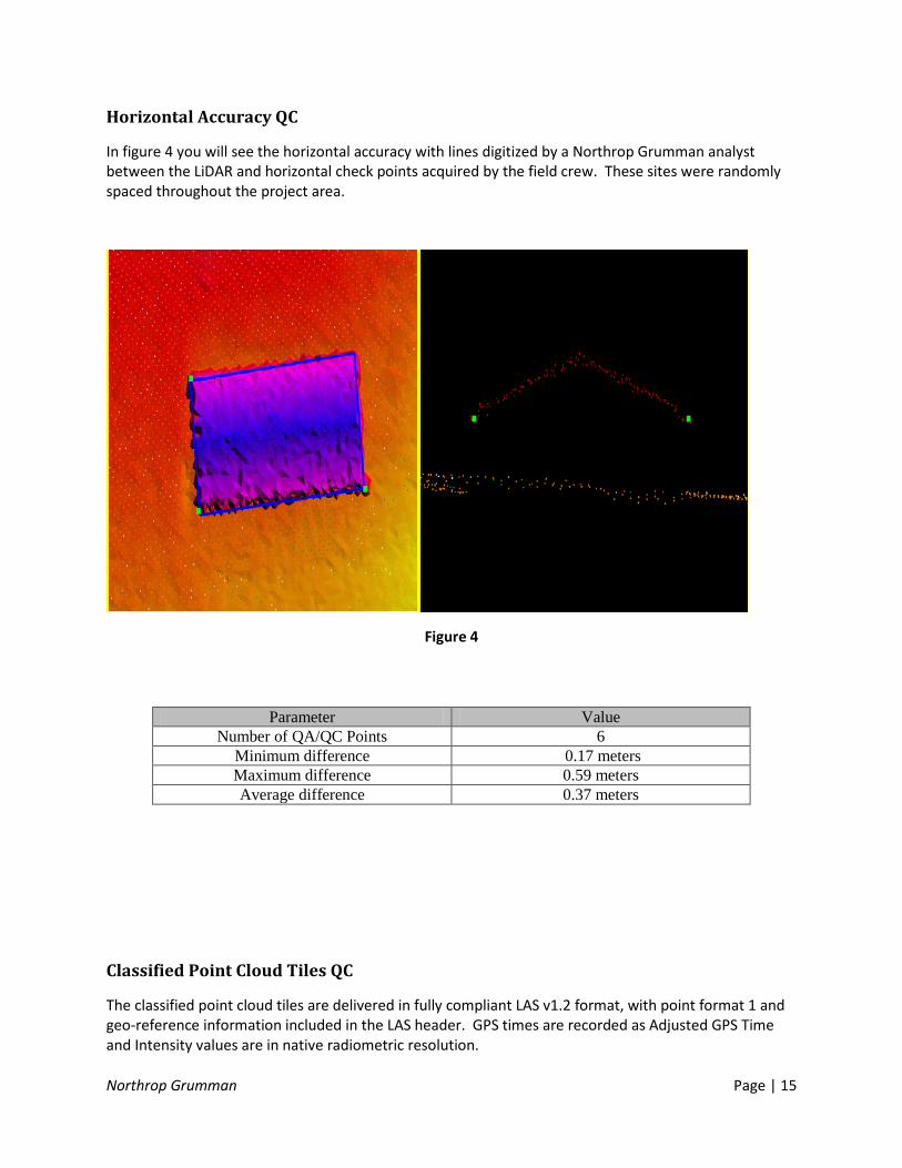
It is worth noting that the ground returns are not necessarily smooth in a surface model. Due to the excellent ground penetration by the sensor, there is much detail to the terrain and "Ground" point class, as seen in Figure 5:

Figure 5

The apparent roughness of the ground point class does appear to accurately represent the ground returns by the sensor. As a result, there are bumps and ridges in the ground class that may initially appear as noise, but have been determined to be actual ground returns.

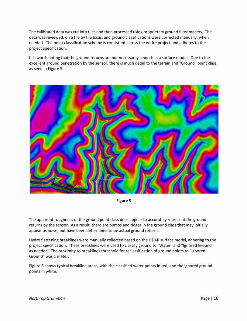
Hydro flattening breaklines were manually collected based on the LiDAR surface model, adhering to the project specification. These breaklines were used to classify ground to "Water" and "Ignored Ground" as needed. The proximity to breaklines threshold for reclassification of ground points to "Ignored Ground" was 1 meter.

Figure 6 shows typical breakline areas, with the classified water points in red, and the ignored ground points in white:


Figure 6

The classified tiles went through one round of Quality Control (QC), point classification edits and breakline collection using experienced LiDAR analysts. A second round of QC was performed by our most experienced analysts, which sometimes involved minor edits to the point classifications and breaklines. If a major problem was found with an analyst's work, corrections were made, submitted back to the analyst for correction. These corrections were then reviewed by the final QC analyst to ensure that the correction was made and that the data now meets the project specification.

While the classified point cloud tiles were reviewed by viewing surface models on a tile by tile basis, the point classifications were also checked in a DEM mosaic, a surface analysis hillshade view, for any noticeable anomalies.

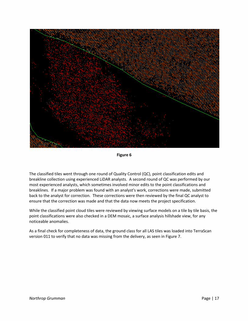
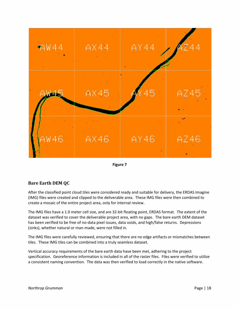
As a final check for completeness of data, the ground class for all LAS tiles was loaded into TerraScan version 011 to verify that no data was missing from the delivery, as seen in Figure 7.


Figure 7

Bare Earth DEM QC

After the classified point cloud tiles were considered ready and suitable for delivery, the ERDAS Imagine (IMG) files were created and clipped to the deliverable area. These IMG files were then combined to create a mosaic of the entire project area, only for internal review.

The IMG files have a 1.0 meter cell size, and are 32-bit floating point, ERDAS format. The extent of the dataset was verified to cover the deliverable project area, with no gaps. The bare earth DEM dataset has been verified to be free of no-data pixel issues, data voids, and high/false returns. Depressions (sinks), whether natural or man-made, were not filled in.

The IMG files were carefully reviewed, ensuring that there are no edge artifacts or mismatches between tiles. These IMG tiles can be combined into a truly seamless dataset.

Vertical accuracy requirements of the bare earth data have been met, adhering to the project specification. Georeference information is included in all of the raster files. Files were verified to utilize a consistent naming convention. The data was then verified to load correctly in the native software.


Breakline QC

All breakline elements were manually collected, using MicroStation v8, in DGN format. All breaklines went through the QC process multiple times alongside the classified point cloud tiles. The breaklines were collected, meeting the requirements for surface area and stream or river width, per the project specifications. The breakline features are seamless between tiles. The breakline height, at any given point, is determined to be at, or just below the immediately surrounding terrain, representing the level of the water surface. All breakline areas are flat and level bank-to-bank and are perpendicular to the apparent flow centerline.

Swath Extent QC

The swath extent shapefile was analyzed for numerical accuracy as well as correct spatial representation. This involved loading the LAS files and visually checking the boundaries that were created. It also required checks throughout the attribute table to verify the correct file naming was applied to each swath's polygon.

Metadata QC

Metadata templates for each product were created by an experienced analyst. Each section of the metadata was analyzed for accuracy and inclusion of all requirements. Upon completion of the metadata templates, the templates were modified slightly to adhere to each products requirements specifically referring to processing steps, product format, and methodology. Finally, the USGS metadata parser was used to validate the metadata against the FGDC Content Standard for Digital Geospatial Metadata.


Conclusion

From the precise flight planning around various environmental and project specific requirements to the rigorous QA/QC process at Northrop Grumman, these LiDAR survey products have been produced to meet or exceed the required specifications according to the statement of work. Great care has been taken to ensure the surveyed data flown between March 01, 2011 and March 09, 2011 is an accurate representation of the ground during these dates.

project report shenandoah 1.0m nps lidar lidar survey

Documents