Wide field and wide band imaging

Tim Cornwell

Overview

• Wide field effects in imaging

• Wide band effects in imaging (largely defer to Urvashi’s talks)

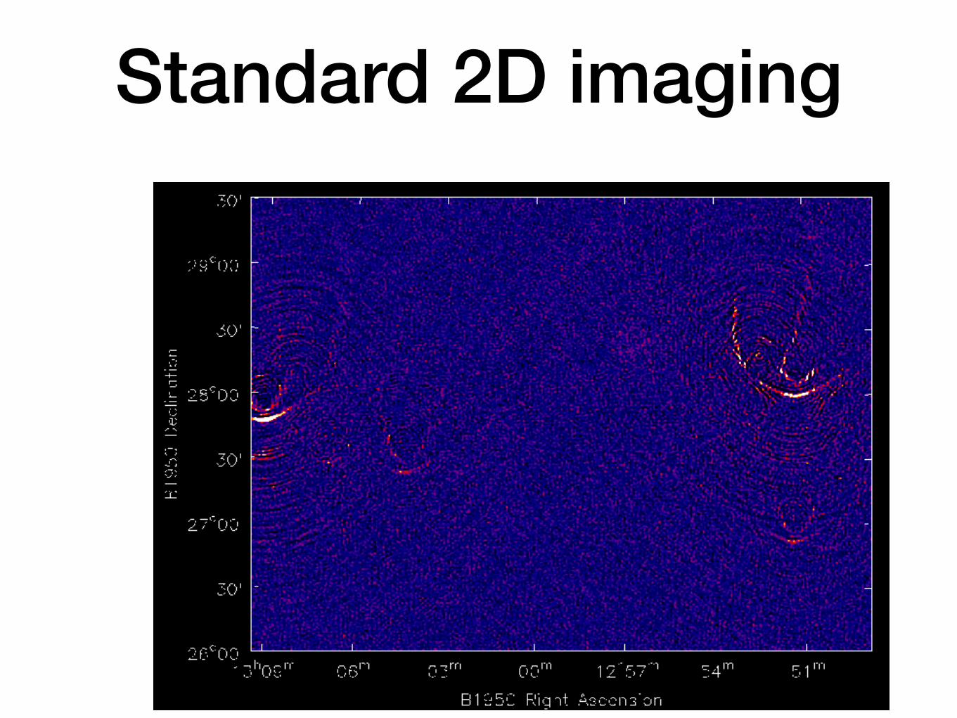
Standard 2D imaging

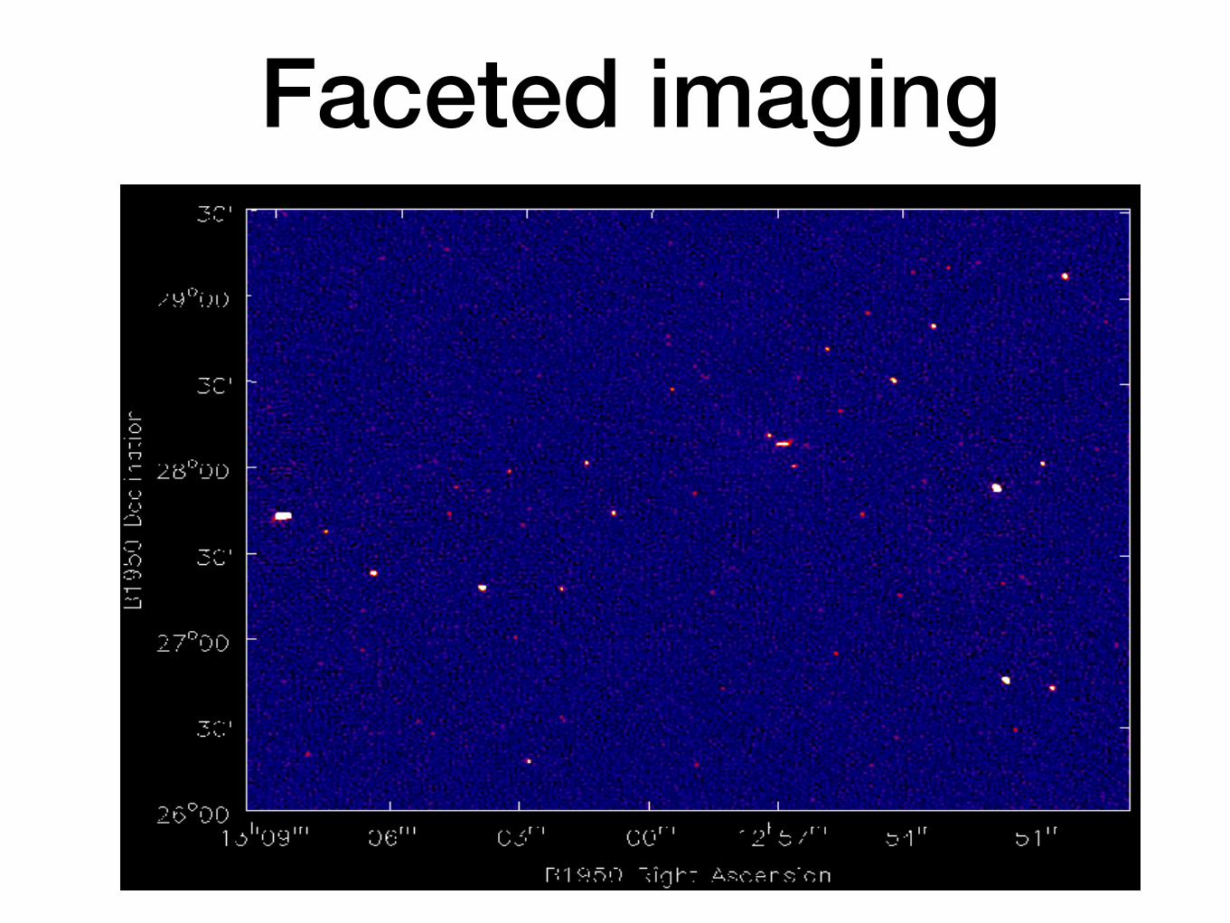
Faceted imaging

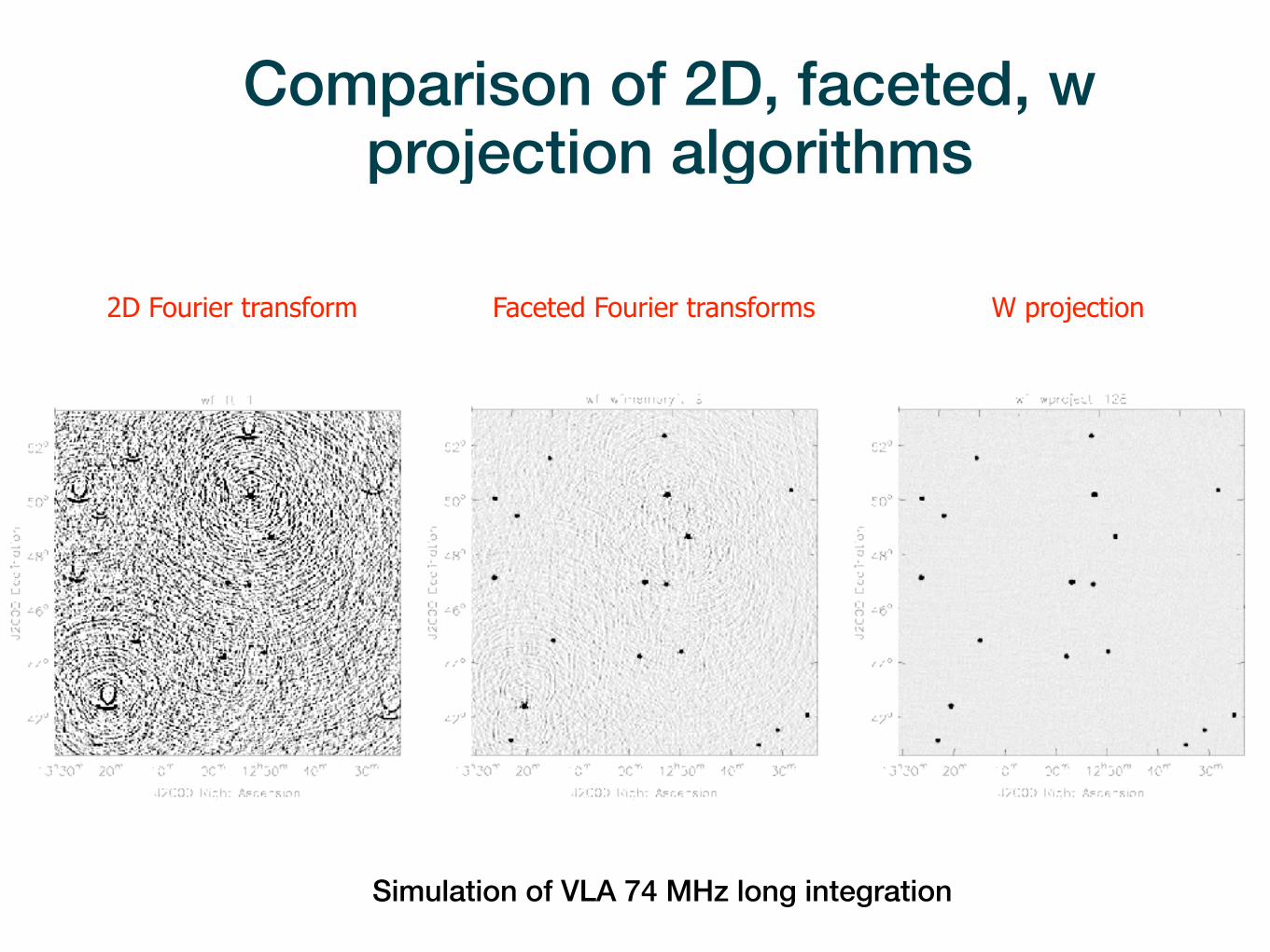
2D Fourier transform Faceted Fourier transforms W projection

Comparison of 2D, faceted, w projection algorithms

Simulation of VLA 74 MHz long integration

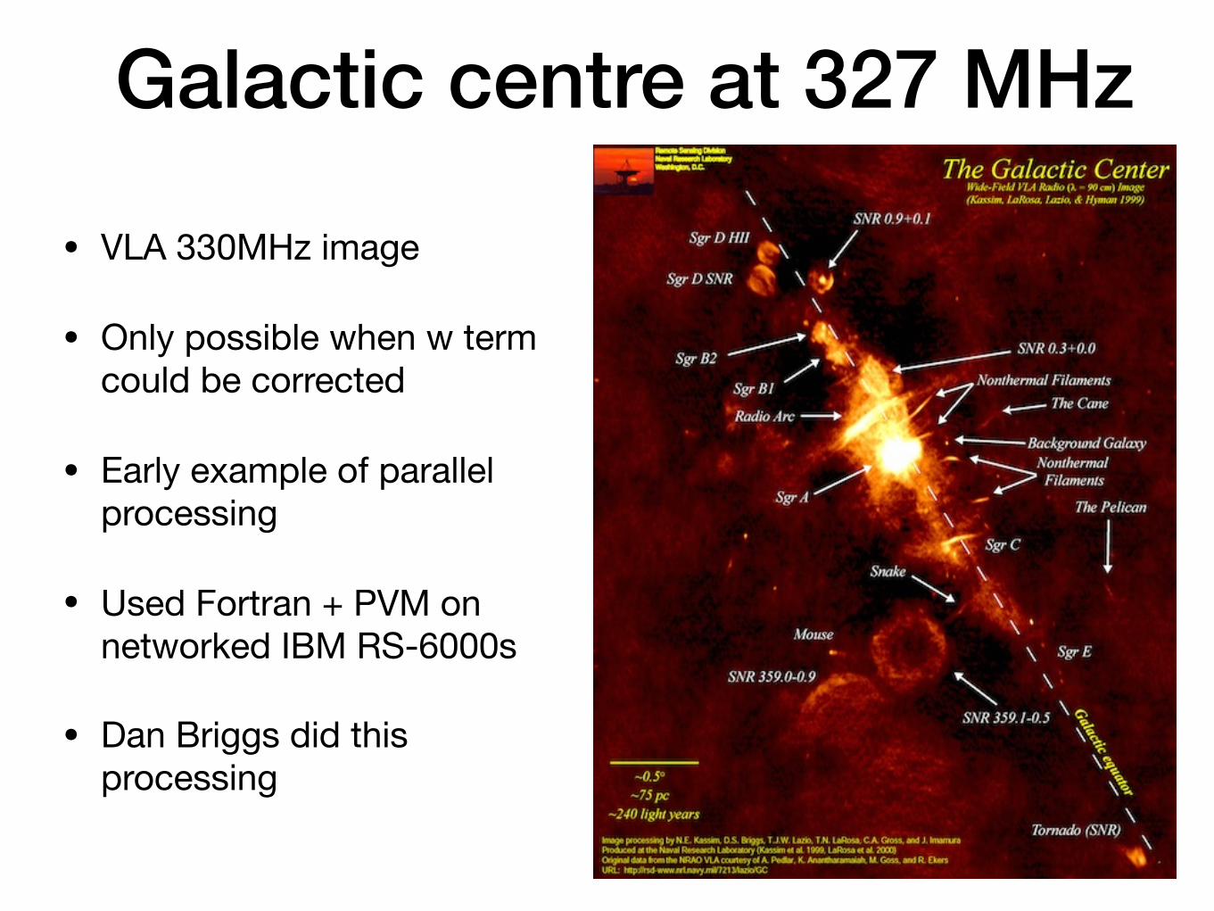
Galactic centre at 327 MHz

• VLA 330MHz image

• Only possible when w term could be corrected

• Early example of parallel processing

• Used Fortran + PVM on networked IBM RS-6000s

• Dan Briggs did this processing

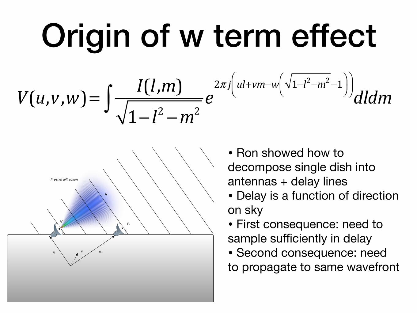
• Ron showed how to decompose single dish into antennas + delay lines• Delay is a function of direction on sky• First consequence: need to sample sufficiently in delay• Second consequence: need to propagate to same wavefront

Origin of w term effect

A

BA'

vu w

Fresnel diffraction

A

BA'

vu w

V(u,v ,w)= I(l ,m)1− l2 −m2

e2π j ul+vm−w 1−l2−m2−1⎛

⎝⎜⎞⎠⎟

⎛⎝⎜

⎞⎠⎟∫ dldm

Can telescope design help?

• Coplanar array e.g. WSRT, ATCA, MWA

• Large antennas/stations

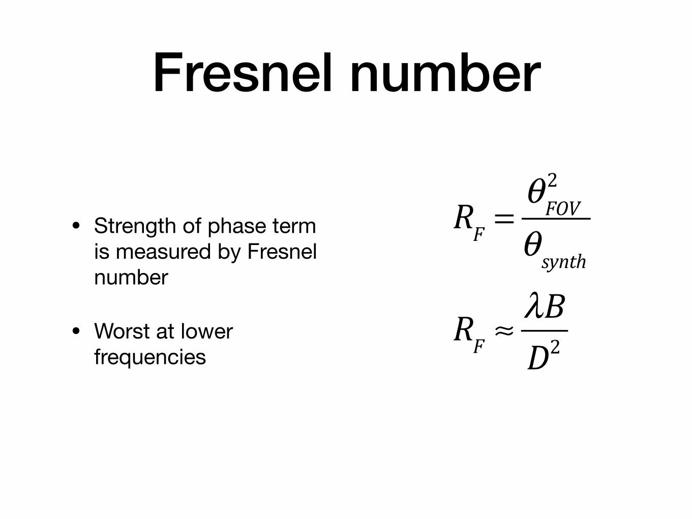
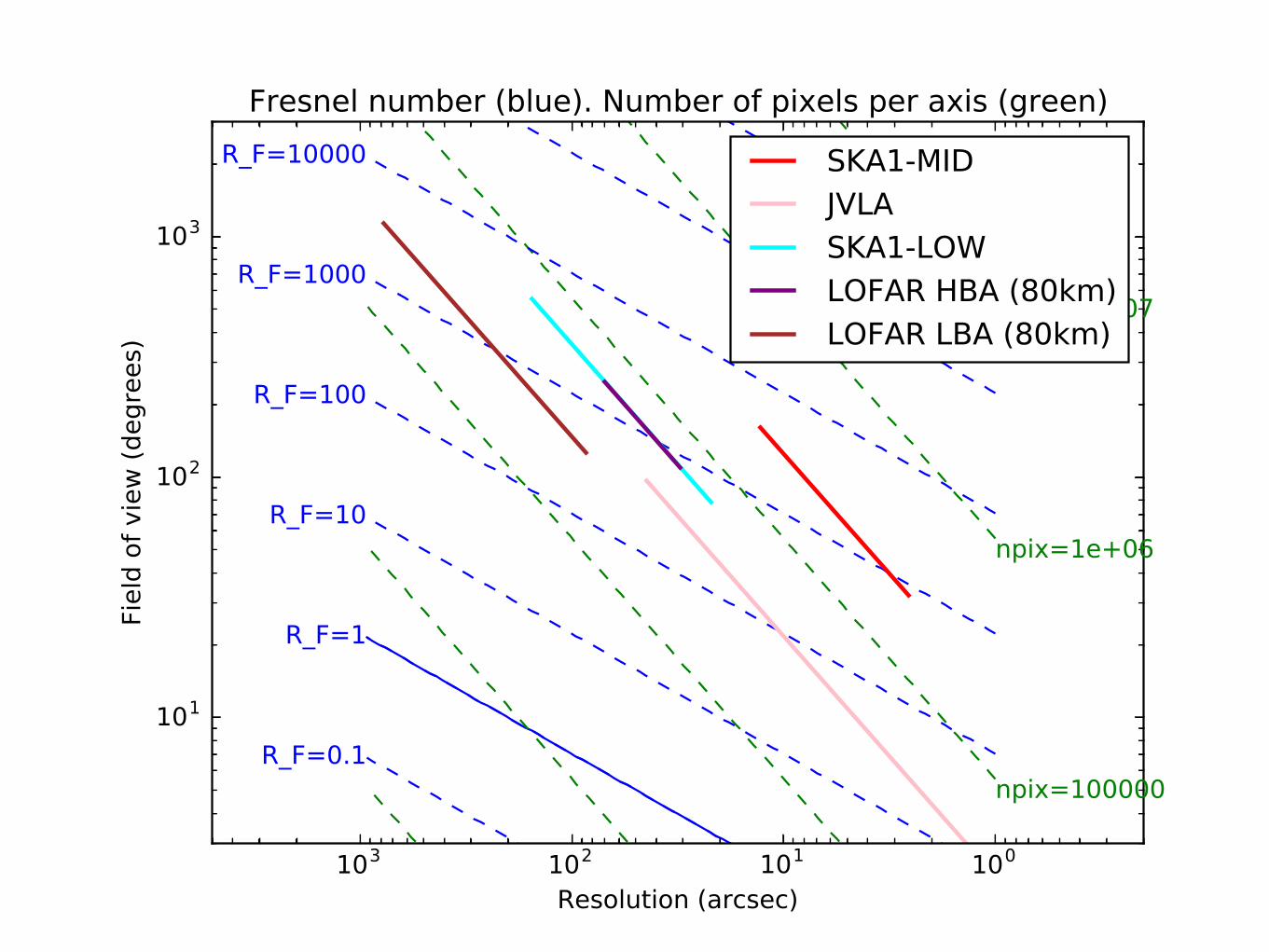
Fresnel number

• Strength of phase term is measured by Fresnel number

• Worst at lower frequencies

RF =θFOV2

θ synth

RF ≈λBD2

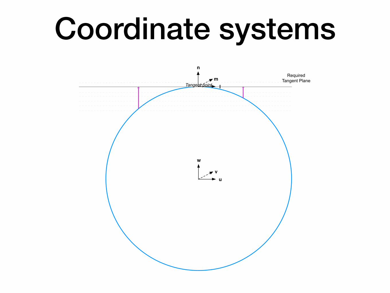
Coordinate systemsRequired

Tangent PlaneTangent point

uv

w

lm

n

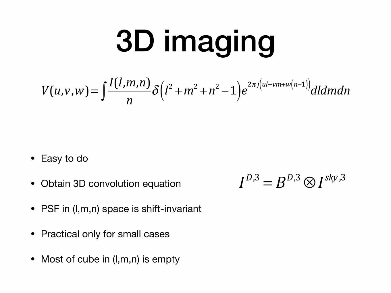
3D imaging

• Easy to do

• Obtain 3D convolution equation

• PSF in (l,m,n) space is shift-invariant

• Practical only for small cases

• Most of cube in (l,m,n) is empty

V(u,v ,w)= I(l ,m,n)n

δ l2 +m2 +n2 −1( )e2π j ul+vm+w n−1( )( )∫ dldmdn

ID ,3 = BD ,3⊗ I sky ,3

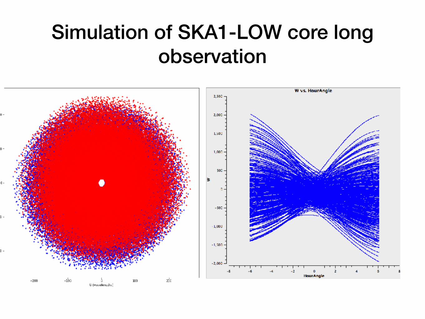
Simulation of SKA1-LOW core long observation

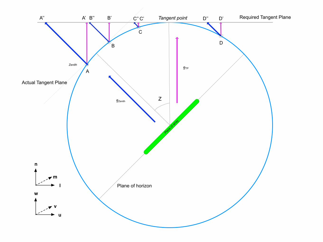
Required Tangent Plane

eTP

eZenith Z

A

B

C

A’’ B’’ C’’

Plane of horizon

Tangent point

Zenith

Plane o

f arra

y

B’ C’A’ D’’

D

D’

Actual Tangent Plane

u

v

wl

m

n

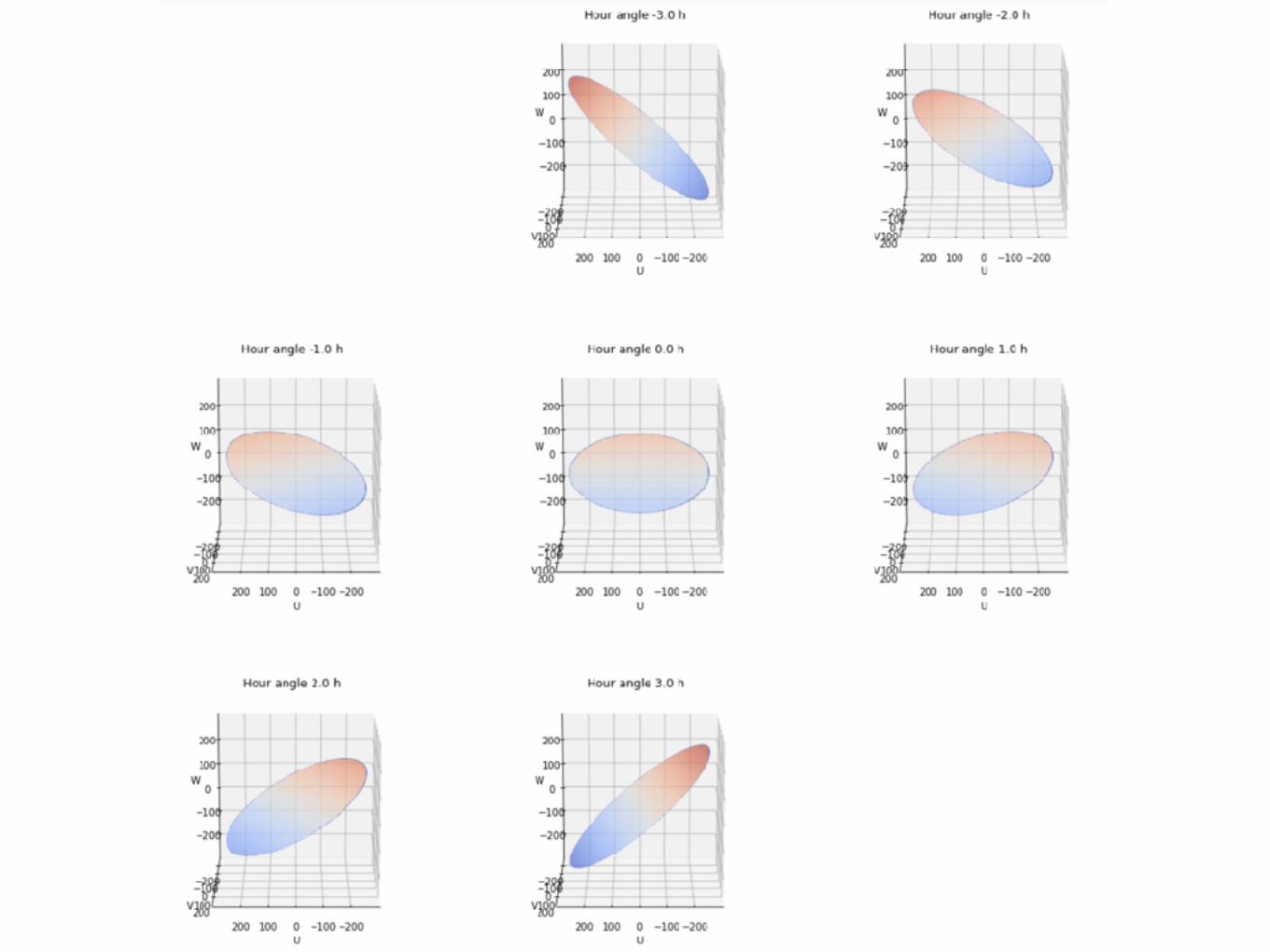
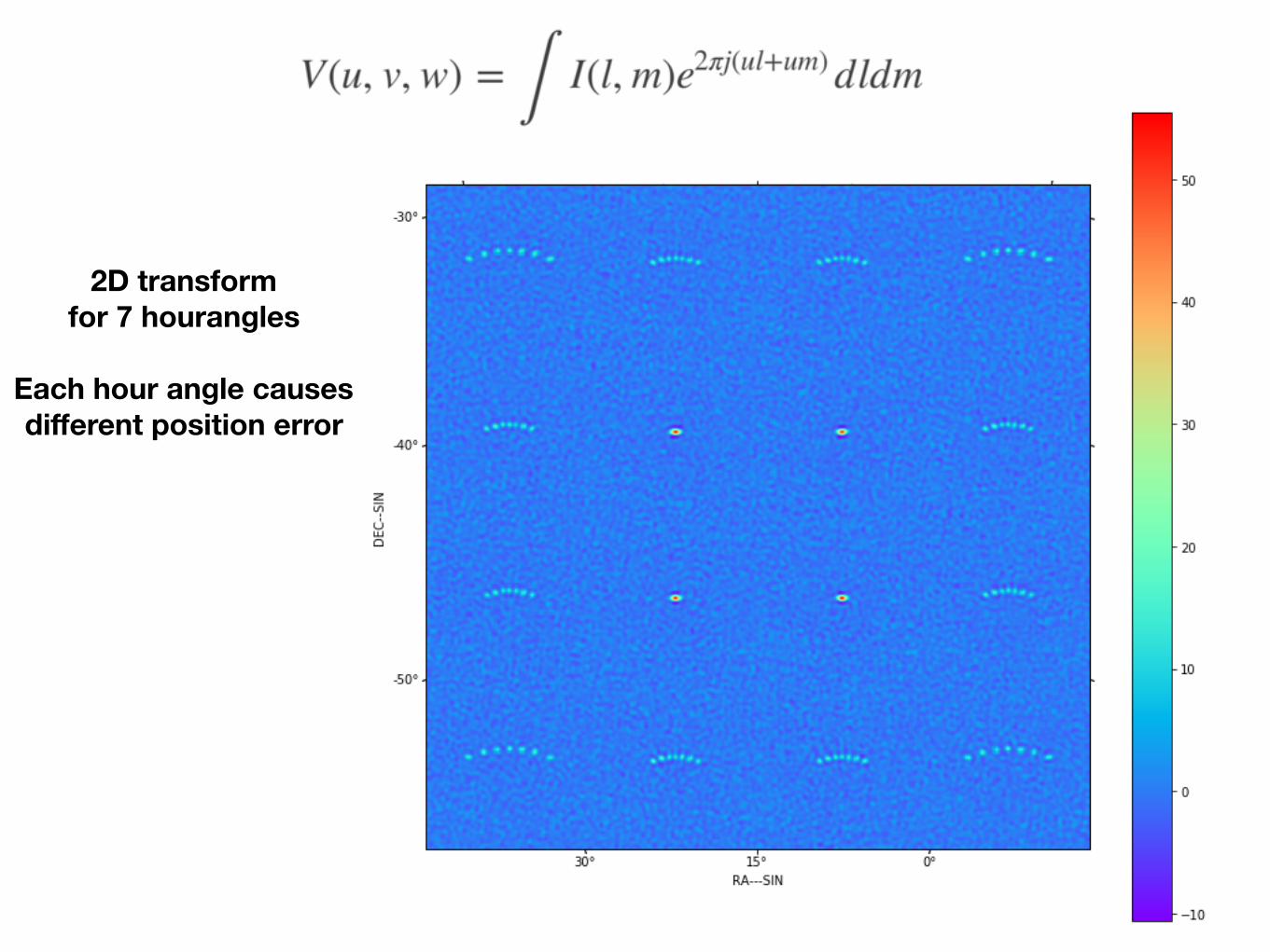
2D transform for 7 hourangles

Each hour angle causes different position error

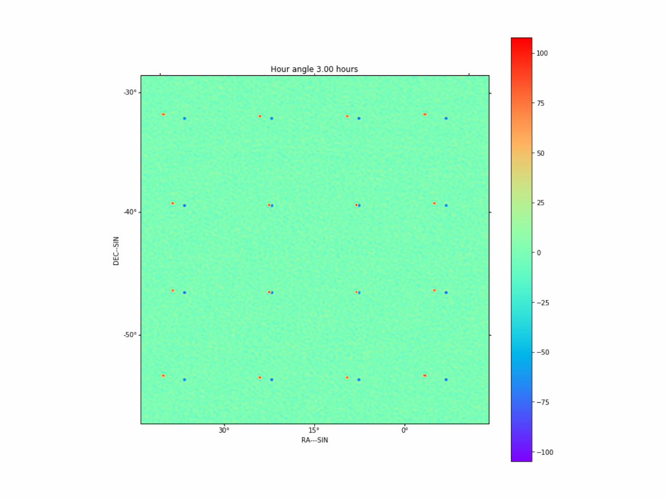
2D transform for 7 hourangles

Each hour angle causes different position error

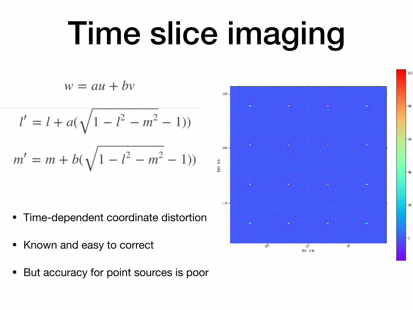
Time slice imaging

• Time-dependent coordinate distortion

• Known and easy to correct

• But accuracy for point sources is poor

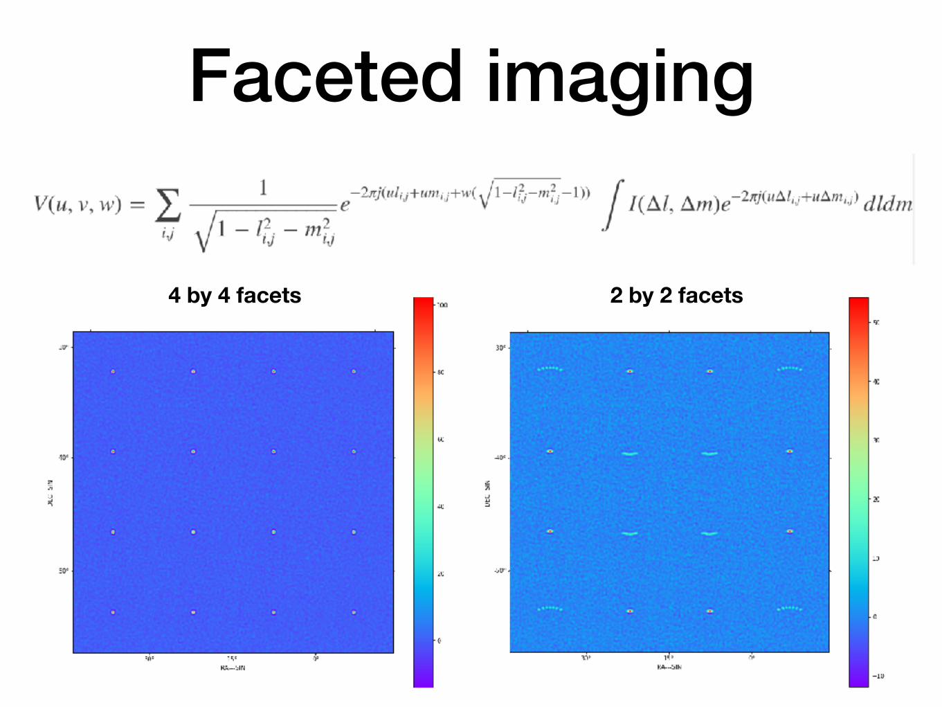
4 by 4 facets

Faceted imaging

2 by 2 facets

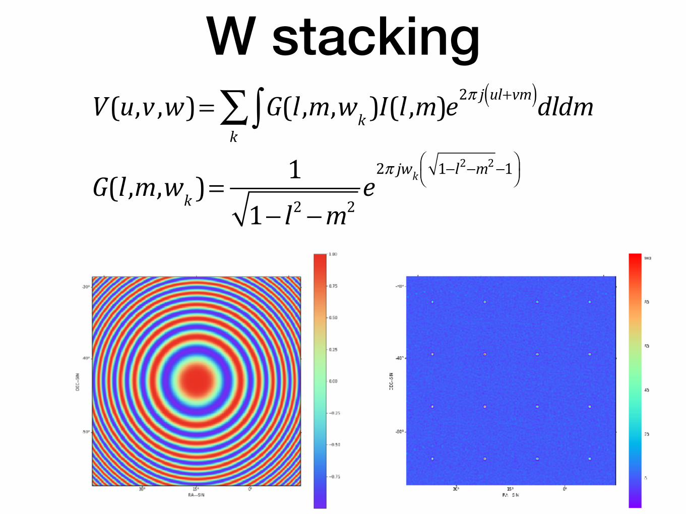
W stackingV(u,v ,w)= G(l ,m,wk )I(l ,m)e

2π j ul+vm( )∫ dldmk∑

G(l ,m,wk )=1

1− l2 −m2e2π jwk 1−l2−m2−1⎛

⎝⎜⎞⎠⎟

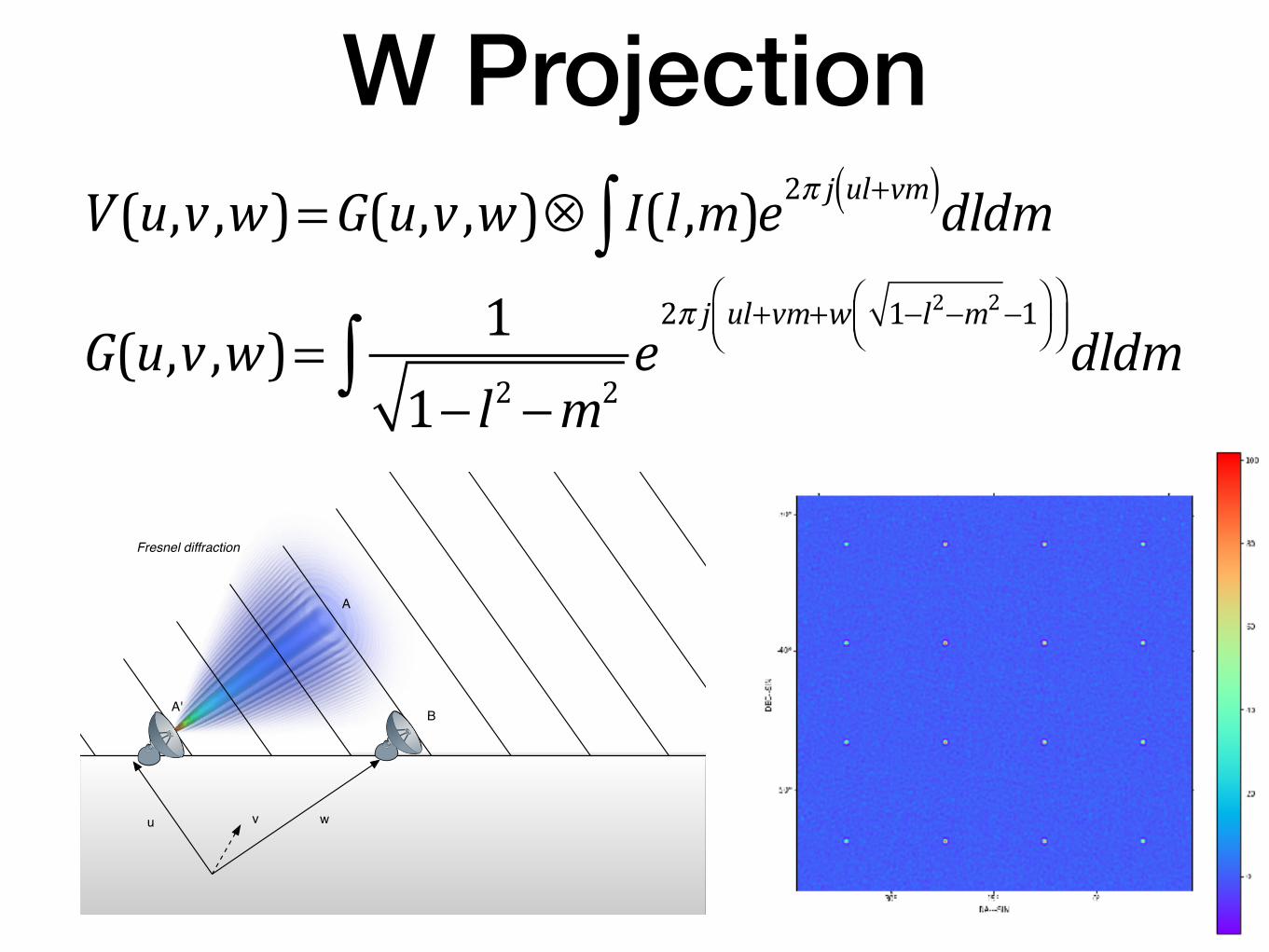
W Projection

Fresnel diffraction

A

BA'

vu w

V(u,v ,w)=G(u,v ,w)⊗ I(l ,m)e2π j ul+vm( )∫ dldm

G(u,v ,w)= 11− l2 −m2

e2π j ul+vm+w 1−l2−m2−1⎛

⎝⎜⎞⎠⎟

⎛⎝⎜

⎞⎠⎟∫ dldm

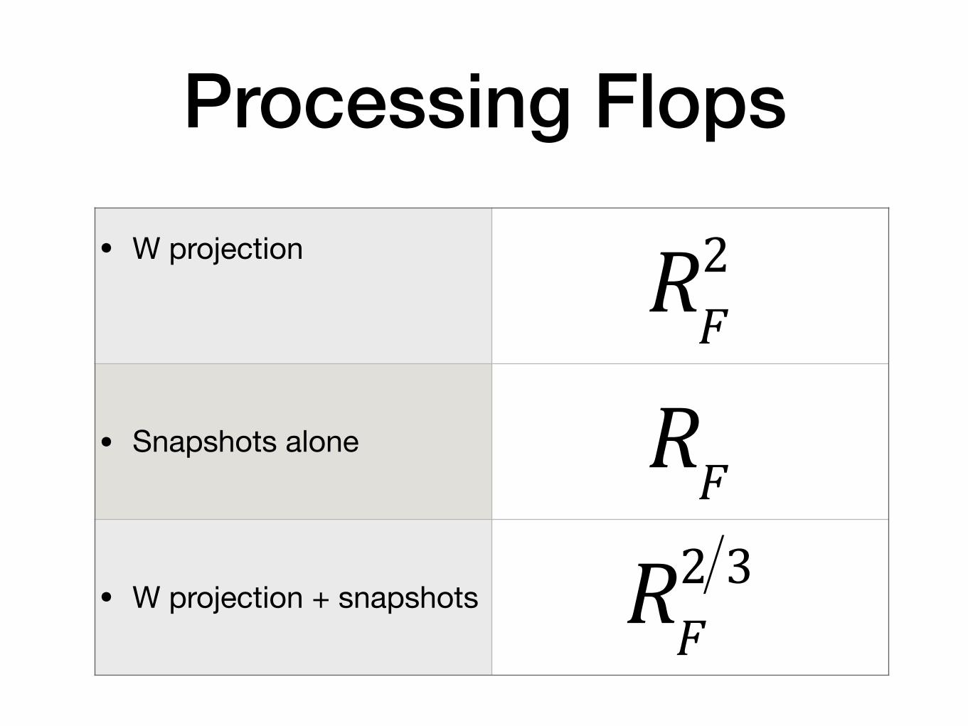
Processing Flops

RF2

RFRF2 3

• W projection

• Snapshots alone

• W projection + snapshots

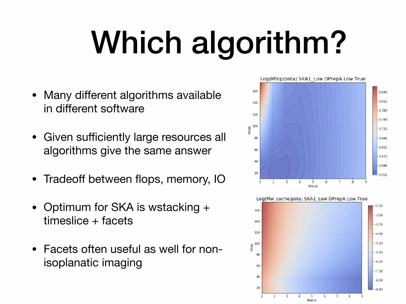
Which algorithm?• Many different algorithms available

in different software

• Given sufficiently large resources all algorithms give the same answer

• Tradeoff between flops, memory, IO

• Optimum for SKA is wstacking + timeslice + facets

• Facets often useful as well for non-isoplanatic imaging

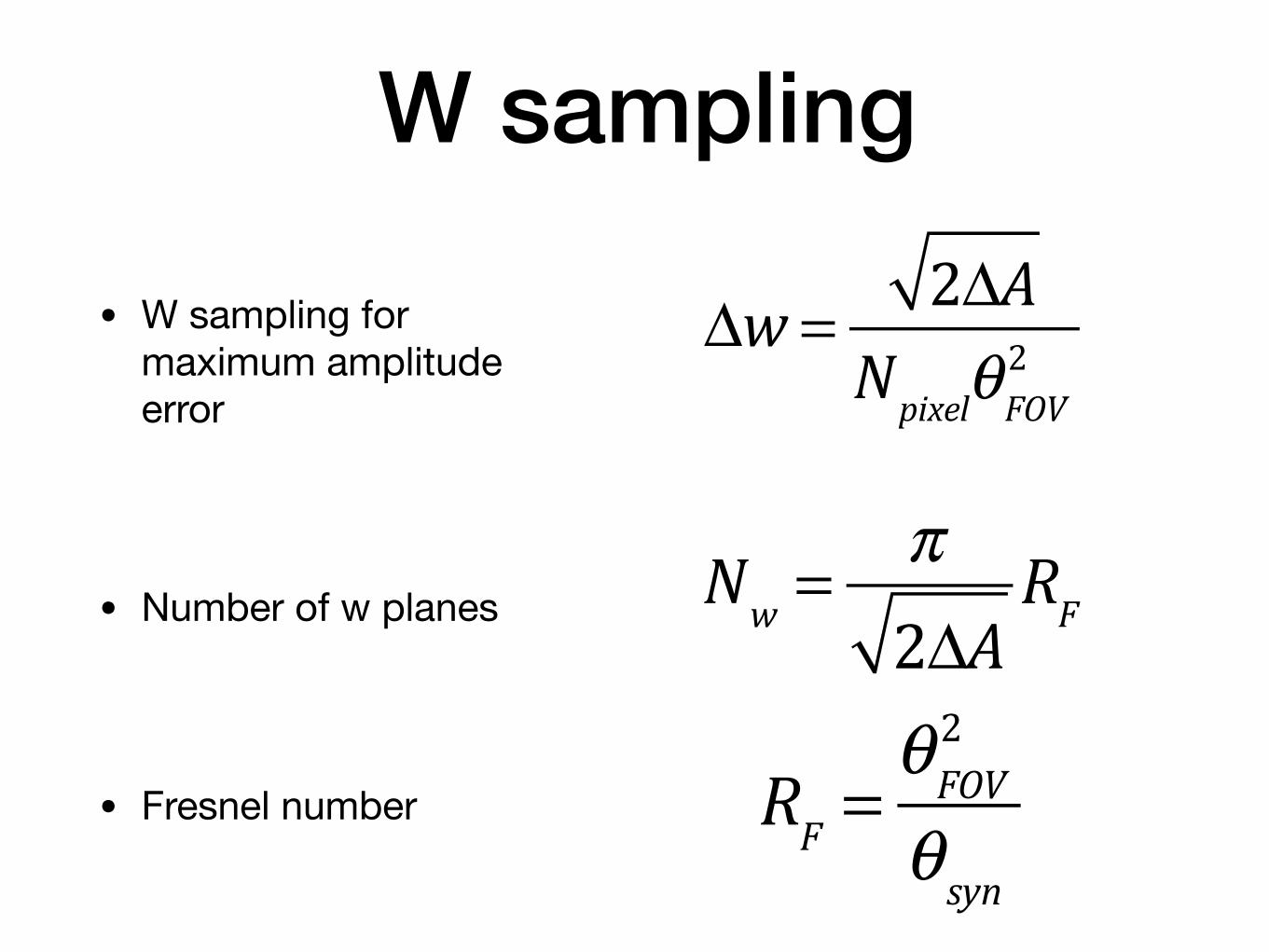
W sampling

• W sampling for maximum amplitude error

• Number of w planes

• Fresnel number

Δw = 2ΔANpixelθFOV

2

Nw =π2ΔA

RF

RF =θFOV2

θ syn

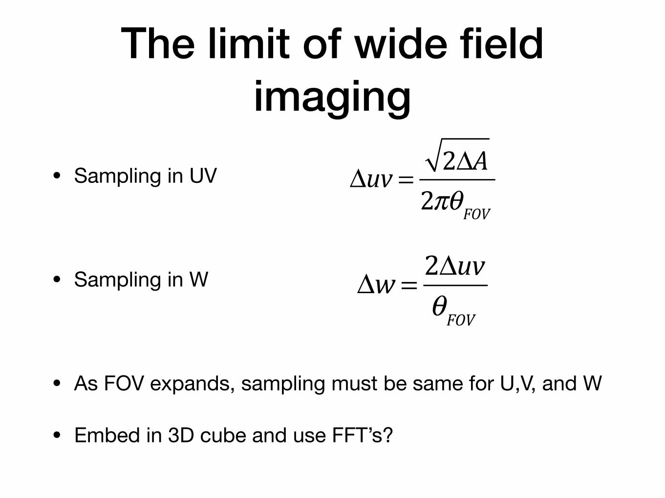
The limit of wide field imaging

• Sampling in UV

• Sampling in W

• As FOV expands, sampling must be same for U,V, and W

• Embed in 3D cube and use FFT’s?

Δuv = 2ΔA2πθFOV

Δw = 2ΔuvθFOV

Wide bandwidth imaging• Improving UV coverage improves the quality of imaging

• Both UV coverage and sensitivity scale with frequency

• But sources change with frequency

• And primary beam changes with frequency

• Need to solve for both image at some frequency plus change with frequency

• e.g. Taylor expansion in frequency

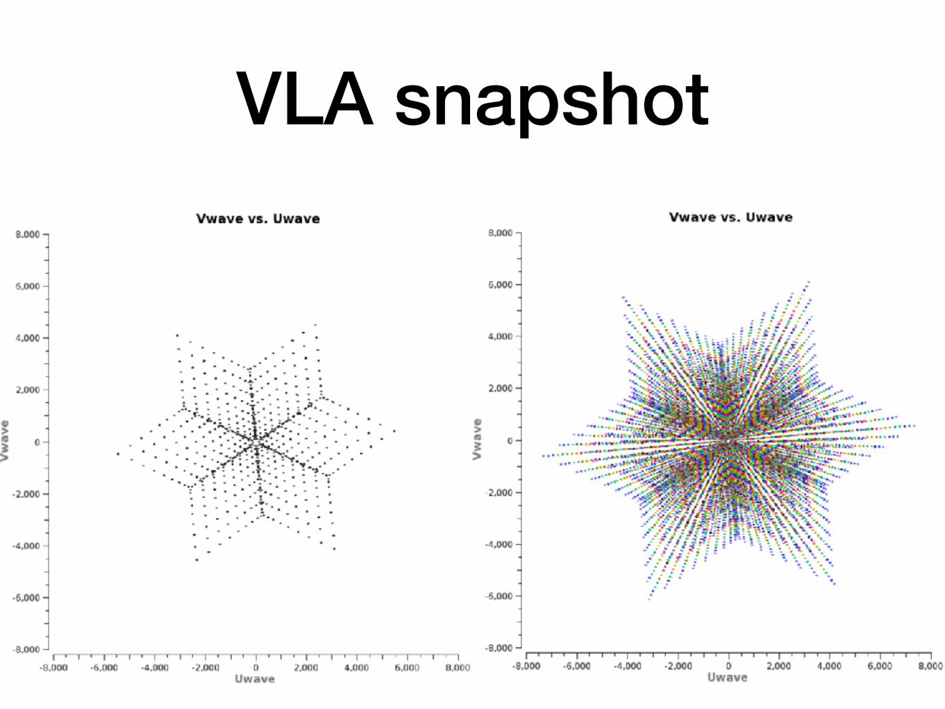
VLA snapshot

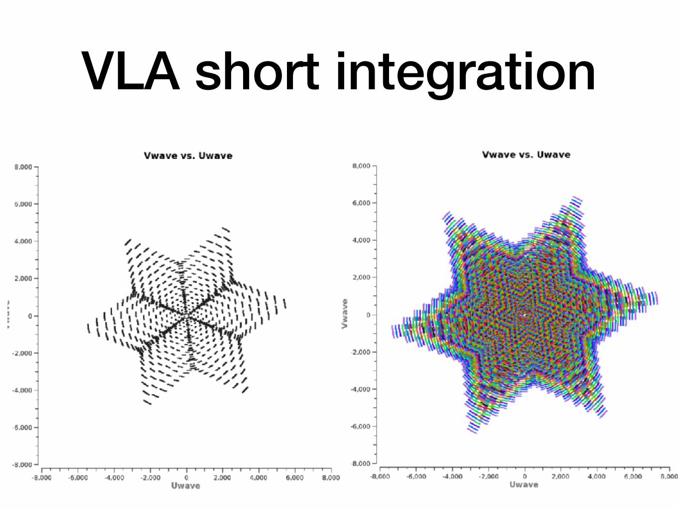
VLA short integration

15th NRAO Synthesis Imaging Workshop, 1-8 June 2016 5

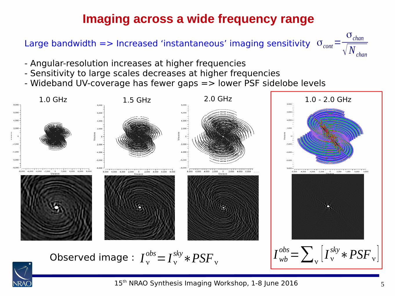
Imaging across a wide frequency range

1.0 GHz 1.5 GHz 2.0 GHz 1.0 - 2.0 GHz

Large bandwidth => Increased ‘instantaneous’ imaging sensitivity

- Angular-resolution increases at higher frequencies- Sensitivity to large scales decreases at higher frequencies- Wideband UV-coverage has fewer gaps => lower PSF sidelobe levels

I wb

obs=∑ν[ I ν

sky∗PSF ν ]I νobs= I ν

sky∗PSF νObserved image :

σcont=σchan

√Nchan

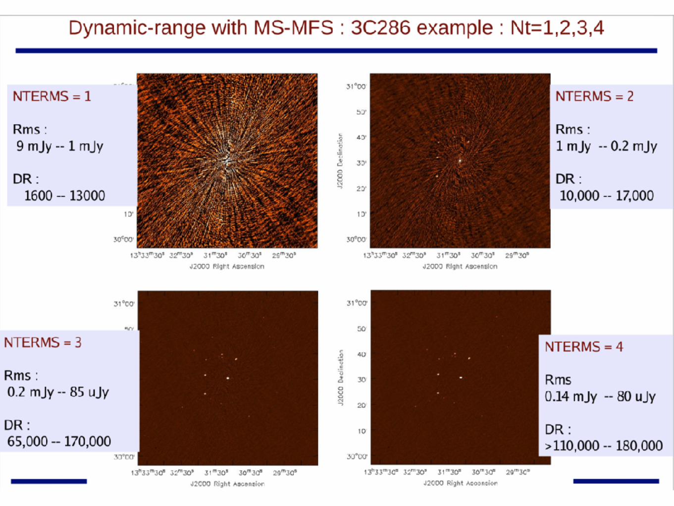
Algorithms

• Sault-Wieringa algorithm Clean, first order in frequency

• Rau algorithm, multiscale, n order expansion in frequency

More information

• Urvashi Rau Ph.D. thesis

• Urvashi Rau RAS talk, 2012