the two wide-angle imaging neutral-atom … two wide-angle imaging neutral-atom spectrometers...
TRANSCRIPT

Space Sci Rev (2009) 142: 157–231DOI 10.1007/s11214-008-9467-4
The Two Wide-angle Imaging Neutral-atomSpectrometers (TWINS) NASA Mission-of-Opportunity
D.J. McComas · F. Allegrini · J. Baldonado · B. Blake · P.C. Brandt · J. Burch ·J. Clemmons · W. Crain · D. Delapp · R. DeMajistre · D. Everett · H. Fahr ·L. Friesen · H. Funsten · J. Goldstein · M. Gruntman · R. Harbaugh · R. Harper ·H. Henkel · C. Holmlund · G. Lay · D. Mabry · D. Mitchell · U. Nass · C. Pollock ·S. Pope · M. Reno · S. Ritzau · E. Roelof · E. Scime · M. Sivjee · R. Skoug ·T.S. Sotirelis · M. Thomsen · C. Urdiales · P. Valek · K. Viherkanto · S. Weidner ·T. Ylikorpi · M. Young · J. Zoennchen
Received: 28 July 2008 / Accepted: 17 November 2008 / Published online: 16 January 2009© Springer Science+Business Media B.V. 2008
Abstract Two Wide-angle Imaging Neutral-atom Spectrometers (TWINS) is a NASA Ex-plorer Mission-of-Opportunity to stereoscopically image the Earth’s magnetosphere for thefirst time. TWINS extends our understanding of magnetospheric structure and processesby providing simultaneous Energetic Neutral Atom (ENA) imaging from two widely sepa-rated locations. TWINS observes ENAs from 1–100 keV with high angular (∼4° × 4°) andtime (∼1-minute) resolution. The TWINS Ly-α monitor measures the geocoronal hydro-
D.J. McComas (�) · F. Allegrini · J. Burch · J. Goldstein · R. Harbaugh · C. Pollock · S. Pope ·M. Reno · C. Urdiales · P. Valek · S. Weidner · M. YoungSouthwest Research Institute, 6220 Culebra Road, San Antonio, TX 78238-5166, USAe-mail: [email protected]
J. Baldonado · D. Delapp · D. Everett · H. Funsten · R. Harper · R. Skoug · M. ThomsenLos Alamos National Laboratory, Bikini Atoll Road SM30, Los Alamos, NM 87545, USA
B. Blake · J. Clemmons · W. Crain · L. Friesen · D. Mabry · M. SivjeeThe Aerospace Corporation, 2350 El Segundo Blvd., El Segundo, CA, USA
P.C. Brandt · R. DeMajistre · D. Mitchell · E. Roelof · T.S. SotirelisApplied Physics Laboratory, Johns Hopkins University, Johns Hopkins Road, Laurel, MD, 20723-6099,USA
H. Fahr · G. Lay · U. Nass · J. ZoennchenArgelander Institute for Astronomy, Astrophysics Section, University of Bonn, Auf dem Huegel, 53121Bonn, Germany
M. GruntmanAstronautics and Space Technology Division, University of Southern California, Los Angeles, CA90089-1192, USA
H. Henkelvon Hoerner & Sulger GmbH, Schlossplatz 8, 68723 Schwetzingen, Germany

158 D.J. McComas et al.
gen density to aid in ENA analysis while environmental sensors provide contemporaneousmeasurements of the local charged particle environments. By imaging ENAs with identicalinstruments from two widely spaced, high-altitude, high-inclination spacecraft, TWINS en-ables three-dimensional visualization of the large-scale structures and dynamics within themagnetosphere for the first time. This “instrument paper” documents the TWINS design,construction, calibration, and initial results. Finally, the appendix of this paper describesand documents the Southwest Research Institute (SwRI) instrument calibration facility; thisfacility was used for all TWINS instrument-level calibrations.
Keywords Energetic neutral atom imaging · ENA · ENA instrumentation ·Magnetosphere · Geocorona · Space plasma calibration facility
PACS 94.80.+g · 94.30.C2 · 94.30.Lr · 94.30.Va
Acronym List
ACE: Advanced Composition ExplorerAMU: Atomic Mass UnitBESSY II: Berlin Electron SynchrotronBLOB: Binary Large ObjectCAPS: Cassini Plasma SpectrometerCEM: Channel Electron MultiplierCHAMPs: Charge PreamplifiersCRCM: Comprehensive Ring Current ModelCTL: ControlDBS: Database ServerDE: Dynamics Explorer spacecraftDOS: DosimeterDOY: Day of YearDP: Data ProcessingDPU: Data Processing UnitDST: Disturbance Storm Time: a measure of the Earth’s magnetic field
disturbanceEBOX: Electronics BoxEEPROM: Electrically Erasable Programmable Read-Only MemoryEMI: Electromagnetic InterferenceENA: Energetic Neutral AtomEPO: Education and Public OutreachES: Environmental SensorESD: Electrostatic DischargeESTL: European Space Tribology Laboratory
C. Holmlund · K. Viherkanto · T. YlikorpiVTT, Tietotie 3, 02044 Espoo, Finland
S. RitzauBurle Electro-Optics, Inc., P.O. Box 1159, Sturbridge, MA 01566, USA
E. ScimeDepartment of Physics, West Virginia University, Morgantown, WV 26506, USA

The Two Wide-angle Imaging Neutral-atom Spectrometers (TWINS) 159
FEE: Front-End ElectronicsFM: Flight ModelFOV: Field-of-ViewFWHM: Full Width at Half MaximumFPGA: Field Programmable Gate ArraysGSE: Ground Support EquipmentGSM: Geocentric Solar MagnetosphericHENA: High Energy Neutral Atom imager on IMAGEHVPS: High Voltage Power SuppliesIES: Ion Electron SensorIMAGE: Imager for Magnetopause-to Aurora Global Exploration SpacecraftIMF: Interplanetary Magnetic FieldIDL: Interactive Data LanguageIO: Input/OutputJFET: Junction Field Effect TransistorLAD: Lyman-α DetectorLAM: Latch-Actuating MechanismLANL: Los Alamos National LaboratoryLEMMS: Low Energy Magnetospheric Measurements SystemLENA: Low Energy Neutral Atom Instrument on IMAGELISM: Local Interstellar MediumLLD: Low Level DiscriminatorLVPS: Low Voltage Power SuppliesMAG: Magnetometer InstrumentMCP: Micro-Channel PlateMENA: Medium Energy Neutral Atom Instrument on IMAGEMIT: Massachusetts Institute of TechnologyMLI: Multi-Layer InsulationMLT: Magnetic Local TimeMoO: Mission-of-OpportunityMPA: Magnetospheric Plasma Analyzer instrument on a series
of geosynchronous spacecraftMRI-VIDEOS: Multi-point Magnetospheric Reconnaissance Imagine: Visualization
of Ion Dynamics, Evolution, Origins, and StructuresNASA: National Aeronautics and Space AdministrationNSSDC: National Space Science Data CenterPEM: Parameterized Exospheric ModelPHA: Pulse Height AnalyzerPWM: Pulse-Width ModulatorRGA: Residual Gas AnalyzerRTD: Resistive Temperature DetectorsS/C: SpacecraftSCM: Surface-Charging MonitorSDS: Science Data SystemSOC: Science Operations CenterSOLSTICE: Solar Stellar IRadiance Comparison ExperimentSoHO: Solar and Heliospheric ObservatorySQL: Structured Query LanguageSRAM: Static Random Access Memory

160 D.J. McComas et al.
SWAN: Solar Wind ANisotropy Instrument on SoHOSwRI: Southwest Research InstituteTCP/IP: Transmission Control Protocol/Internet ProtocolTOF: Time of FlightTWA: TWINS ActuatorTWINS: Two Wide-angle Imaging Neutral-atom Spectrometers Mission
of OpportunityUARS: Upper Atmosphere Research SatelliteUNIX: UNiplexed Information and Computing SystemUPS: Uninterruptible Power SupplyUT: Universal TimeWUI: Web User-InterfaceWTA: Wax Thermal Actuator
Contents
1 Introduction . . . . . . . . . . . . . . . . . . . . . . . . . . . . . . . . . . . . . . . 1611.1 Background and Overview . . . . . . . . . . . . . . . . . . . . . . . . . . . . . 1611.2 TWINS Scientific Objectives . . . . . . . . . . . . . . . . . . . . . . . . . . . 167
2 TWINS Instrumentation . . . . . . . . . . . . . . . . . . . . . . . . . . . . . . . . . 1702.1 Mechanical System . . . . . . . . . . . . . . . . . . . . . . . . . . . . . . . . . 1712.2 Electrical System . . . . . . . . . . . . . . . . . . . . . . . . . . . . . . . . . . 1732.3 ENA Sensor Heads . . . . . . . . . . . . . . . . . . . . . . . . . . . . . . . . . 1752.4 Lyman-α Detector (LAD) . . . . . . . . . . . . . . . . . . . . . . . . . . . . . 1842.5 DPU and Electronics . . . . . . . . . . . . . . . . . . . . . . . . . . . . . . . . 1872.6 TWINS Actuator (TWA) . . . . . . . . . . . . . . . . . . . . . . . . . . . . . . 1922.7 TWINS Environmental Sensor . . . . . . . . . . . . . . . . . . . . . . . . . . . 197
3 Calibration and Instrument Performance . . . . . . . . . . . . . . . . . . . . . . . . 1993.1 Detector (Gain) . . . . . . . . . . . . . . . . . . . . . . . . . . . . . . . . . . . 2013.2 FOV and Angular Mapping . . . . . . . . . . . . . . . . . . . . . . . . . . . . 2023.3 TOF Determination . . . . . . . . . . . . . . . . . . . . . . . . . . . . . . . . . 2043.4 Mass Identification . . . . . . . . . . . . . . . . . . . . . . . . . . . . . . . . . 2053.5 Geometric Factor . . . . . . . . . . . . . . . . . . . . . . . . . . . . . . . . . . 2063.6 Collimator Response . . . . . . . . . . . . . . . . . . . . . . . . . . . . . . . . 2073.7 Calibration Summary . . . . . . . . . . . . . . . . . . . . . . . . . . . . . . . . 208
4 TWINS Data and Science Analysis . . . . . . . . . . . . . . . . . . . . . . . . . . 2084.1 TWINS Science Data . . . . . . . . . . . . . . . . . . . . . . . . . . . . . . . . 2084.2 The TWINS Science Operations Center and Science Data System (SDS) . . . 2104.3 Achieving Closure on TWINS Science Objectives . . . . . . . . . . . . . . . . 2114.4 Inversion of TWINS ENA Images to Extract Global Energetic Ion Distributions 211
5 Initial Stereo Observations from TWINS-1 and -2 . . . . . . . . . . . . . . . . . . 2146 Conclusions . . . . . . . . . . . . . . . . . . . . . . . . . . . . . . . . . . . . . . . 218Acknowledgements . . . . . . . . . . . . . . . . . . . . . . . . . . . . . . . . . . . . 218Appendix A: The Southwest Research Institute Instrument Calibration Facility . . . . 219
A.1 Introduction . . . . . . . . . . . . . . . . . . . . . . . . . . . . . . . . . . . . . 219A.2 Vacuum System and Lab Layout . . . . . . . . . . . . . . . . . . . . . . . . . 219A.3 Ion Source and Optics . . . . . . . . . . . . . . . . . . . . . . . . . . . . . . . 221A.4 Positioning System . . . . . . . . . . . . . . . . . . . . . . . . . . . . . . . . . 223

The Two Wide-angle Imaging Neutral-atom Spectrometers (TWINS) 161
Appendix B: Inversion of Individual ENA images . . . . . . . . . . . . . . . . . . . . 224References . . . . . . . . . . . . . . . . . . . . . . . . . . . . . . . . . . . . . . . . . 227
1 Introduction
The Two Wide-angle Imaging Neutral-atom Spectrometers (TWINS) mission stereoscop-ically images the Earth’s magnetosphere for the first time. TWINS was proposed in June1997 against NASA AO 97-OSS-03 and, after selection, confirmed in April 1999. The hostspacecraft ultimately launched in 2006 and 2008, with routine stereo operations beginningin June 2008. Mission operations are currently funded through FY10 with data analysis sup-port through FY11. This paper details the design and development of the TWINS mission.Section 1 provides a scientific background for TWINS’ science objectives. Section 2 de-scribes the instrument and sensor characteristics with respect to mechanical, electrical andsoftware design. Calibration and instrument performance are described in Sect. 3; a descrip-tion of the SwRI calibration facility and its role in the TWINS calibration is included inAppendix A. TWINS data acquisition, distribution, archiving and analysis are detailed inSect. 4. Section 5 includes initial stereo observations of TWINS-1 and -2.
1.1 Background and Overview
The feasibility of magnetospheric imaging using energetic neutral atoms (ENAs), whicharise from the charge-exchange process between cold geocoronal neutral hydrogen and thelocal energetic ion populations, was first demonstrated two decades ago (Roelof 1987). Thesimple equation for the flux of ENAs jena is
jena =∫
dl nHjionσ (1)
where nH is the neutral hydrogen density in the geocorona, σ is the charge-exchange crosssection, jion is the ion intensity, and the line-of-sight integral is taken over path lengthof the emitting volume. Over the past two decades, technologies have been developed toprovide higher sensitivity, better angular resolution, and, most importantly, to extend theobservable ENA energy range below several tens of keV, down to ∼1 keV (McComaset al. 1991, 1998). High energy neutral atom images from NASA’s Polar spacecraft andthe Swedish Astrid microsat provided some of the first tantalizing glimpses of the powerof neutral atom imaging (Henderson et al. 1997, 1999; Barabash et al. 1997). Finally, inMarch 2000 the mid-sized Explorer, IMAGE, (Burch 2000) was launched into its high-altitude, high-inclination orbit. IMAGE has provided a full range of ENA observations ofthe magnetosphere with three complimentary ENA imaging instruments: HENA (Mitchellet al. 2000) covering ∼20–500 keV, MENA (Pollock et al. 2000) covering ∼1–30 keV,and LENA (Moore et al. 2000) covering ∼10–300 eV. Since then, a broad range of scien-tific studies have used these observations and demonstrated the power of ENA imaging inunderstanding our dynamic magnetosphere, including substantial contributions to the under-standing of magnetospheric substorms (Pollock et al. 2003, and references therein; Huanget al. 2003) and storms (Brandt et al. 2001; Pollock et al. 2001; McComas et al. 2002;Skoug et al. 2003; Moore et al. 2003; Perez et al. 2004a, 2004b; Reeves et al. 2003;De Majistre et al. 2004; Roelof et al. 2004, 2005; Vallat et al. 2004; Henderson et al. 2006;Zaniewski et al. 2006; Denton et al. 2005, 2007).

162 D.J. McComas et al.
From the solid foundation of magnetospheric observations carried out with ENAs fromIMAGE, TWINS will extend our understanding of magnetospheric structures and processesby providing simultaneous images from two widely separated locations. The primary obser-vations are neutral atom images from 1–100 keV (extended from MENA’s 1–30 keV energyrange to cover the widely used low energy end of the HENA range) with high temporal(∼1-minute) and spatial (∼ 4◦ × 4◦) resolution. In addition, TWINS’ Lyman-α imager al-lows us to continuously monitor the geocorona, which provides the cold charge-exchangeneutrals that produce the ENAs. Finally, environmental sensors on the TWINS S/C willmake simultaneous measurements of the charged particle environment around the space-craft.
1.1.1 MENA Observations
Because the TWINS imagers are based so closely on the IMAGE/MENA instrument, it isuseful to briefly review a few of the images and results from this instrument. An early andimportant result from MENA demonstrated a high degree of asymmetry in the Earth’s ringcurrent with respect to magnetic local time during the main phase of a geomagnetic storm,followed by a transition to a symmetric and less intense ring current during the storm’s re-covery phase (Pollock et al. 2001). This is due to the strong electric field-driven convectionof plasma during the storm’s main phase that pushes plasma to the magnetopause whereit escapes into the magnetosheath. By contrast, when the storm drivers subside and the re-covery is in progress, the convection is weaker, ion drift paths close to completely encirclethe Earth, and the ring current plasma becomes trapped. Figure 1 shows observations of ageomagnetic storm on August 12, 2000 (Pollock et al. 2001).
The notion that the magnetosphere may be primed for large storms by the presence ofa super-dense plasma sheet received convincing support from the work of McComas et al.(2002), who used MENA imagery integrated over the GSM-Y dimension to demonstrate thecorrelation between enhanced MENA emissions from the mid-tail region and the advent oflarge magnetic storms (see Fig. 2). That study demonstrated that ENA emissions could beroutinely observed back to several tens of RE deep in the magnetotail when IMAGE wasin an appropriate orbital position. Enhanced emissions (high plasma sheet densities) wereassociated with high solar wind densities and with super dense plasma sheet observations atgeosynchronous orbit. These authors examined two magnetospheric storm intervals whereplasma sheet loading began prior to the storms and continued under all IMF BZ orientations,reaching its maximum during the peaks of the storms. For several days following these
Fig. 1 MENA observations and magnetospheric activity from August 12, 2000. The three panels show ob-servations from the main phase, early recovery phase, and late recovery phase of a magnetospheric storm,respectively. From Pollock et al. (2001)

The Two Wide-angle Imaging Neutral-atom Spectrometers (TWINS) 163
Fig. 2 Combined figure showing MENA observation of the mid-tail plasma sheet, taken from McComas etal. (2002). The top panel shows the IMAGE spacecraft location in the GSM X–Z plane on 5 October 2000(time in UT hours is labeled along the orbit track). Each spacecraft spin, MENA’s field of view (dark grey)sweeps down the plasma sheet (yellow). The bottom panel shows observations from 21 September (DOY265) through 11 October (DOY 285) 2000. The colored bars provide integrated 1–70 keV ENA emissions asa function of look direction down the tail (right axis), while the white curves show Dst (top, left axis) and IMFBZ (bottom, left axis). The observations from 5 October (top) are highlighted by the vertical yellow outline
storms, ENA emissions were weak, indicating that the plasma sheet remains depleted afterthe storms.
Another technique, developed by Scime et al. (2002), used spatially resolved MENA en-ergy spectra to derive magnetospheric temperature maps that compared favorably with con-current in situ observations of the hot ion plasma at geosynchronous orbit (Figs. 3 and 4).Subsequent determination of equatorial ion temperatures through inversions of the sameMENA data also compared favorably with the in situ observations (Zhang et al. 2005). How-

164 D.J. McComas et al.
Fig. 3 Twenty-minute averaged ion temperature images from MENA from August 12, 2000. Geomagneticdipole field lines are shown for L = 4 and L = 8 at MLTs = 6, 12, 18, and 24 hours, with the noon field linesdrawn in red. The black dots show the location of the 1994-84 MPA spacecraft at (a) 12:00 UT, (b) 12:30UT, and (c) 13:00 UT. From Scime et al. (2002)
Fig. 4 Smoothed total iontemperature derived from the1994-84 MPA instrument (solidline) in geosynchronous orbitcompare favorably with remotelymeasured ion temperatures fromMENA data (solid circles with±500 eV error bars) . FromScime et al. (2002)
ever, in regions where in situ measurements were not available, the two analysis methodsyielded different ion temperatures. Scime et al. (2002) found higher ion temperatures on thedusk side during storm main phase while the Zhang et al. (2005) found no dusk–dawn iontemperature anisotropy.
Ring current models, such as the Fok et al. (1995) three-dimensional (3-D) ring currentdecay model, include Coulomb collisions and charge-exchange losses while bounce averag-ing the kinetic equation for the ion distribution function. In terms of ion transport in a largestorm, the Fok et al. (1995) model predicted that during the recovery phase, ions would sep-arate according to energy. Less energetic ions (below ∼3 keV) co-rotate eastward and arelost to charge-exchange collisions in the dawn and pre-noon sectors. High energy (>30 keV)ions follow the gradient-curvature drift westward. The result is a peak of high energy ions inthe dusk sector, isolated from the low energy ions that peak on the dawn side. In terms of iontemperatures, higher ion temperatures would then be expected in the dusk region comparedto the dawn region. The Jordanova et al. (1997) model, which includes wave–particle in-teractions, losses due to charge-exchange collisions, Coulomb collisions, and plasma wavescattering along ion drift paths also predicts a dawn–dusk asymmetry in ion flux, with in-creased ion flux in the dusk region becoming more pronounced with ion energy. Newer ring

The Two Wide-angle Imaging Neutral-atom Spectrometers (TWINS) 165
current models, such as the Comprehensive Ring Current Model (CRCM) (Fok et al. 2003;Ebihara et al. 2004) that calculate the electric field self-consistently by computing the elec-tric potential when the ring current is allowed to close through a model of ionospheric con-ductance, suggest that predictions of enhanced densities of energetic ions near dusk dependstrongly on the strength of the convective electric field in the inner magnetosphere. There-fore, dawn–dusk ion temperature asymmetries could be an indicator of strong convectiveelectric fields.
Zaniewski et al. (2006) built on this thermal mapping capability, applying superposedepoch analysis to 39 storms and derived magnetospheric temperature maps at different sub-storm phases (Figs. 5 and 6). They found that there are significant differences between thespatial distribution of ion fluxes and ion heating during the main phase of storms. Analysesof ENA images at a single energy clearly emphasize the dynamics and structure of densityenhancements, while energy resolved or energy spectra analysis is more likely to highlightmicroscopic phenomena such as wave–particle interactions and ion heating or macroscopicphenomena such as energetic ion convection from the nightside. On average, a large en-hancement of ENA emission appears across a wide range of magnetic local time (MLT) onthe night side during the main phase of the storms. At higher ENA energies, the enhance-ment is localized to a small region that is slightly post-midnight—consistent with previousHENA observations and image inversions. Ion temperature images indicate that the ENA
Fig. 5 Averaged ENA flux images projected into common coordinates for mainphase storm intervals atenergies of (a) 4.0 keV, (b) 6.0 keV, (c) 9.0 keV, (d) 13.0 keV, (e) 20.0 keV, and (f) 32.5 keV. In eachEarth-centered image, the Sun is to the right and L = 2 and L = 4 dipole magnetic field lines are shown.From Zaniewski et al. (2006)

166 D.J. McComas et al.
Fig. 6 (a) pre-storm, (b) main,(c) early recovery, (d) laterecovery ion temperature imagesaveraged over 39 storms in aformat similar to Fig. 5. Thewhite arrows show the directionsof the spacecraft–Earth vectorsused in each superposed imagewith the length of the arrowsindicating the projection of thespacecraft–Earth vector in theequatorial plane. The ENA fluxesused to create (b) are shown inFig. 5. From Zaniewski et al.(2006)
enhancement arises from an influx of relatively cold plasma. Significant ion heating is ob-served on the dayside of the inner magnetosphere at 5–6 RE (RE is earth radius) out from theEarth at the same time. During the early recovery phase, the ion temperature on the daysidedrops to approximately 9 keV and a colder region of approximately 6.5 keV persists nearpre-dawn. In the late recovery phase of the storm, the ion temperature throughout the innermagnetosphere appears to relax to a nearly uniform 8 keV (Fig. 6).
In another recent study, Pollock et al. (2004) examined the peculiar nature of MENAemissions from low altitude. These emissions coincide with energetic proton precipitationinto the atmosphere at a limited band of latitudes near or slightly equatorward of aurorallatitudes. A small fraction of these protons are reflected back into space, presumably aftermultiple interactions with the background exosphere. The peculiarity of these low altitudeENA emissions follows from the fact that they are emitted from near the top of the atomicoxygen exobase into a relatively narrow band of barely escaping magnetic pitch angles at theemission site. The result is a non-homogeneous (spatially banded) distribution of ENA fluxin space. Simultaneous observation from the two TWINS spacecraft will greatly enhanceour ability to use these emissions to specify the global ion precipitation into the atmosphere.
1.1.2 TWINS Stereo Observations
The great success of the IMAGE mission is a credit to the scientists making the most ofsingle-vantage-point observations. However, such images can only be interpreted by makingassumptions about the ion pitch angle distributions and/or 3-D spatial distributions. In con-trast, the TWINS mission was conceived and designed to provide ENA observations simul-taneously from two vantage points, thus allowing resolution of 3-D plasma structures and

The Two Wide-angle Imaging Neutral-atom Spectrometers (TWINS) 167
Fig. 7 Notional sketch of theMolniya orbits of the twoTWINS spacecraft
ion pitch-angle distributions. The need for stereoscopic imaging of the magnetosphere wasidentified early when the MRI-VIDEOS study (Mitchell et al. 1993) was selected in responseto a 1996 Announcement of Opportunity to study advanced mission concepts suitable for fu-ture Sun–Earth Connections missions. The TWINS mission concept benefited substantiallyfrom the MRI-VIDEOS study. This study also demonstrated the value of such a mission tothe scientific community and led to NASA’s 1997 Sun–Earth Connections roadmap explic-itly including a dedicated “Stereo Magnetospheric Imager” mission in its Solar–TerrestrialProbes mission set.
It is significant that TWINS provides closure on a large fraction of the MRI-VIDEOSand Stereo Magnetospheric Imager science for a small fraction of the cost of an independentstereo imaging mission. This substantial cost savings was enabled with TWINS primarilyby flying the TWINS instrumentation as a Mission-of-Opportunity (MoO) on two high-inclination, high-altitude spacecraft. We refer to these “host” spacecraft simply as TWINSS/C-1 and TWINS S/C-2.
The host spacecraft are in Molniya orbits with inclinations of 63.4◦, perigee altitudes of∼1000 km, and apogees in the northern hemisphere at ∼7.2 RE (Fig. 7). Molniya orbits areunique because they maintain a fixed argument of perigee. The orbit has a period of onehalf of a sidereal day, giving two fixed geographic longitudes for alternate apogees. TheTWINS spacecraft are 3-axis stabilized and provide approximately nadir pointing surfacesthat the TWINS instruments sit on. Such an arrangement is ideal for the TWINS scientificgoals, since the imagers rotate about an axis pointed roughly towards the Earth at all timesand thus will always observe the magnetosphere. The orbits are similar to that optimizedfor magnetospheric imaging on IMAGE, providing a unique opportunity to obtain stereoimages of the magnetosphere at extremely low cost to NASA. In addition, because the twospacecraft have a significant offset in their orbital phases (apogees at different times), thepair can provide nearly continuous magnetospheric observations in addition to simultaneous,dual platform viewing for a portion of each orbit. Data from both spacecraft are provided tothe science community via our web site (http://twins.swri.edu/) as well as ultimately throughthe NSSDC archive. TWINS-1 and -2 observations are routinely available starting in June2008.
1.2 TWINS Scientific Objectives
While TWINS has numerous scientific goals that relate to the various individual regionswhich will be imaged, the primary scientific goal of the TWINS investigation is to estab-lish the global connectivity and causal relationships between processes in different regions

168 D.J. McComas et al.
of the magnetosphere. While IMAGE has taken the first important steps in imaging themagnetosphere, TWINS provides another major step forward by enabling the capability ofunfolding the emission variation along the line-of-sight from the integrated ENA intensitiesobtained from each of the spacecraft. The stereo imaging of TWINS counters a serious dif-ficulty with all magnetospheric imaging carried out to date: that of interpreting structuresin an optically thin medium when viewed from a single vantage point; and greatly reducesthe reliance on simplifying assumptions such as isotropy of the magnetospheric ions whenretrieving the 3-D magnetospheric structure and dynamics from the data.
The broad scientific objectives of TWINS are listed below. They build on the scientificobjectives previously established for IMAGE, and will provide a less model-dependent pathto achieving these goals. The TWINS investigation measurement goals are:
(1) Ion Dynamics: To view the global dynamics, composition, and energization of ionsthroughout the magnetosphere with approximately 1-minute time-resolution using simulta-neously obtained dual-vantage-point images of key magnetospheric components includingthe ring current, inner plasma sheet, near-Earth cross-tail current sheet, the high-latitude,low-altitude extensions of these regions and of the outer magnetosphere, the magnetotail,boundary layers, and cusp.
(2) Plasma Origins and Destinies: To trace the sources, transport, and sinks of plasmapopulations, including solar wind entry at the magnetopause, boundary-layer flows and con-vection patterns, acceleration and heating in the near-Earth plasma sheet, and accelerationof ionospheric plasma in the polar regions.
(3) Magnetospheric Evolution: To observe the evolution of the global magnetosphericstructure as solar-wind coupling and internal processes change the state of the magne-tosphere from quiescence, through moderate (substorms) or extreme (storms) levels of ac-tivity, to relaxation and a return to quiescence.
(4) Magnetospheric Structure: To visualize and map the global configuration and organi-zation of the magnetosphere in three dimensions using stereo imaging, forward modeling,and image inversion.
These measurement goals provide the inputs required to establish the spatial connectionsand temporal causalities between the various magnetospheric components and regions forboth active and inactive states of the magnetosphere. For example, the location in the near-Earth magnetotail current sheet where substorm current disruptions initiate remains elusive,and the timing, as well as the mapping, between the equatorial plane and the auroral zoneis still unknown. Multi-point imaging holds our best hope for finally resolving these fun-damental and long-standing problems by: 1) providing a framework for understanding therole of localized processes in establishing the global magnetospheric configuration and dy-namics, and 2) allowing us to extract quantitative information about the configuration andevolution of global electromagnetic parameters, such as the electric field configurations ofthe inner magnetosphere and the generation of the region 2 magnetic field aligned currentsystem.
Unlike past attempts to achieve these goals via in situ multi-spacecraft studies, stereomagnetospheric imaging provides global, not local, observations. Local observations arelimited by spacecraft positions which 1) often miss critical phenomena by not being injust the ‘right’ place, 2) achieve a good spacecraft configuration for only part of an event,and 3) have ambiguity in the timing between events in different regions. In contrast, TWINSprovides global stereo coverage of the magnetosphere.
The above discussion emphasizes the connectivity and causality aspects of the TWINSscience goals. In addition to these global science goals, TWINS will also address detailedscience issues within the various observed regions:

The Two Wide-angle Imaging Neutral-atom Spectrometers (TWINS) 169
Region 2 Currents Gradients in the pressure distribution of the magnetosphere’s hotplasma population, particularly of the Earth’s Ring Current, drive the Region-2 FieldAligned Currents. Despite their obvious importance to global magnetospheric interactions,there are large holes in our understanding of the global and mesoscale configuration and dy-namics of the plasma sheet and ring current populations. Deficiencies in our knowledge oftheir configurations as they relate to models of region 2 current generation have been noted(Lui et al. 1994). Also, the first published ENA image (Roelof 1987) exhibited a dramaticday/night asymmetry that was shown to be capable of driving field-aligned currents with thesame morphology as the region 2 currents (Roelof 1989). Is this new scenario correct? Howis such a distribution generated, and how is it maintained so that a quasi-stationary region 2current system results?
Ring Current A scientific understanding of ring-current physics revolves around three ele-ments: injection, evolution, and decay (Jordanova et al. 1996). With a significantly improvedability to unfold global ENA images, the stereo imaging from TWINS promises progress inall three areas. First, TWINS greatly reduces spatial and temporal uncertainties regardingthe location and extent of ring-current injections and their relationship to substorms. TWINSalso permits us to follow the global progress of the redistribution of the ring-current ions.Moreover, TWINS allows a direct observation of one of the primary ring-current loss mech-anisms, namely charge-exchange with exospheric neutrals. Thus, TWINS enables us to testdirectly and quantitatively our understanding of the role of charge-exchange in ring-currentdecay, including the temporal sequence and spatial distribution. Moreover, with their modestcomposition capability, sufficient to distinguish the major ring-current constituents, O+ andH+, the TWINS ENA imagers can help resolve issues regarding the spatial and temporaldependence of ring-current composition. TWINS offers the opportunity to examine glob-ally the relationship between the level of geomagnetic activity and ring-current compositionbelow 100 keV, in addition to direct observation of charge-exchange loss rates for the twospecies.
Plasma Sheet Mapping of the ion plasma sheet from the equatorial plane to lower altitudesin the auroral zone can be accomplished through stereographic imaging of the horns of theplasma sheet. The azimuthal structure of these horns and the variation of their size and shapewith geomagnetic activity provide important insight into auroral energization processes andthe 3D distribution of Birkeland currents in the nightside magnetosphere. The visualizationof the 3D spatial and temporal structure of the high-latitude extension of the plasma sheetwill be strongly advanced through the application of TWINS stereo observation techniques.In addition to the high-latitude extension of the plasma sheet, TWINS offers the opportunityto directly visualize substorm ion injections and their spatial and temporal progression. Fur-thermore, the TWINS compositional capability and reduced spatial ambiguities may enablethe exploration of the role of heavy-ion enhancements in multiple substorm initiation (Bakeret al. 1982).
Visualization of the ring-current plasma injection, the evolution of the plasma sheet sizeand location, and the plasma sheet extension to high latitudes allows direct global observa-tion of the transfer of energy from the magnetotail into the earth’s upper atmosphere for thefirst time. Stereo imaging not only enables more robust unfolding of the ion fluxes in theseregions, but also provides more frequent viewing of any given region of interest.
Because stereo images bypass the inherent difficulty in inverting single-perspective, line-of-sight-integrated images, the science return from the TWINS mission can be much greaterthan what could be obtained from any single vantage point. The most important contribution

170 D.J. McComas et al.
to magnetospheric science offered by multipoint magnetospheric imaging from TWINS isits ability to unambiguously determine the connectivity and causal relationships between thedifferent regions by locating the ENA emission regions with a precision not possible from asingle vantage point.
One additional TWINS science objective is made possible by including a Lyman-α im-ager as part of the TWINS instrument. Knowledge of the H-atom geocoronal density isessential to the unfolding of the ion intensity from the measurement of the ENA intensity.However, the observational basis for current geocoronal density models is not extensive.One commonly used model is the Chamberlain-type exosphere derived from a four-year av-erage of Lyman-α observations from the DE-1 spacecraft (Chamberlain and Hunten 1987;Rairden et al. 1986). More recently, Østgaard et al. (2003) analyzed IMAGE Lyman-α ob-servations from the nightside, beyond 3.5 RE. The inclusion of a simple Lyman-α imageron TWINS allows us to monitor the shape and intensity of the geocoronal emissions, pro-viding the specific information about the neutral-H exosphere along the TWINS sensors’lines-of-sight needed to unfold the ENA images. In addition, these observations will pro-vide valuable information in their own right regarding the spatial and temporal behavior ofthe neutral exosphere.
2 TWINS Instrumentation
The TWINS mission maximizes the scientific return while minimizing mission cost andrisk. Our strategy to accomplish this with TWINS was to utilize the state-of-the-art MENAinstrumentation, which was just completing development for the IMAGE mission. We per-formed only limited modifications to enhance the measurement capabilities as well as thoserequired to accommodate this hardware as a mission-of-opportunity on the host spacecraft.
The MENA imager “slit camera” concept (McComas et al. 1998) was originally selectedfrom among several promising ideas for imaging ENAs (McComas et al. 1991, 1994, 1998;Gruntman 1997) largely because it provides a very large aperture, and hence geometric fac-tor, required to properly image ENAs across the critical energy range from ∼1 keV to afew 10 s of keV. The sensor heads and the signal-processing electronics of TWINS, in-cluding signal amplification, trajectory calculation, time-of-flight (TOF) determination, andpulse-height analysis, are nearly identical to those of MENA, minimizing cost and risk. Thelargest difference between MENA and TWINS is in how the viewing plane is scanned acrossthe sky, which is driven by fundamental differences between the spacecraft on which theyare flying. For IMAGE, the spacecraft spin rotates the MENA field-of-view (FOV) acrossthe sky. Because the TWINS spacecraft are 3-axis stabilized, the sensor heads are mountedon a rotating actuator, which sweeps back and forth over an approximately Earth-centeredviewing cone. This cone spans the inner and middle magnetosphere for the majority of eachTWINS orbit. The actuator is nearly identical to one used for the CAPS instrument on theCassini spacecraft at Saturn (Young et al. 2004), again maximizing use of heritage designsfor TWINS.
The top level instrument performance characteristics for TWINS are summarized in Ta-ble 1. TWINS separately images fluxes of hydrogen and oxygen ENAs. Hydrogen ENAsfrom ∼1–100 keV are measured with an angular resolution of 4◦ × 4◦ above ∼10 keV(lower energies and oxygen ENAs are provided at reduced angular resolution). In normalmode, a full image from each of the TWINS is made in 60 s each ∼82 s (including the 22 srequired for the actuator to reverse direction).
The list of spacecraft resources required for the TWINS instruments is given in Table 2.TWINS’ total mass is approximately 18.7 kg, the total power consumption is 25.3 W, and

The Two Wide-angle Imaging Neutral-atom Spectrometers (TWINS) 171
Table 1 TWINS performance
Quantity Performance
Angle FOV ≥2.5 sr centered approximately about nadir from each of 2 S/C
Angle resolution 4◦ × 4◦ for H atoms with energies >10 keV
Energy range 1–100 keV for H atoms (higher energy O is also measured)
Energy resolution �E/E ≤ 1.0 for H atoms
Time resolution Full images in 60 s taken every 82 s
Lifetime >2 years
Species identified H, O (scattering becomes large for O below ∼10 keV)
Instrument geometric factor TWINS1: 8.7 × 10⁻³ cm2 sr
TWINS2: 5.6 × 10⁻³ cm2 sr
Table 2 TWINS spacecraftresources Quantity Value
Mass 18.7 kg
Power 25.3 W
Footprint 57 × 57 × 30 cm
Instantaneous FOV ±70◦ centered on rotation axis
Commanding One 16-bit word
TM rate 50 kbps
the data rate is 50 kbps. The TWINS actuators rotate back and forth through 180◦ in a“windshield-wiper” motion with a constant rotation speed of 3◦ s−1 measuring the full dis-tributions of ENAs in the viewing cone over 60 s.
Figure 8 provides a picture of the TWINS-1 instrument just prior to final flight delivery.The major subsystems of TWINS are all labeled: Toward Sensor Head (viewing back to-ward the DPU box), Away Sensor Head, Lyman-α detector, Electronics box, Sensor HeadMounting Structure, TWINS Actuator (TWA), and Tilt Bracket.
The following subsections cover the mechanical and electrical systems and major sub-systems of TWINS in turn. Sections 2.1 and 2.2 are dedicated to the mechanical and electri-cal systems, respectively. Section 2.3 discusses the development of the ENA sensor heads,and Sect. 2.4 explains the use of the Lyman-α Detector in image inversion. The TWINS-specific design of the Data Processing Unit (DPU) and electronics are described in Sect. 2.5followed by details of the TWINS Actuator (TWA) design in Sect. 2.6. Finally, the envi-ronmental monitors included in the TWINS spacecraft are discussed in Sect. 2.7 TWINSEnvironmental Sensor.
2.1 Mechanical System
The design of the mechanical system was driven by the requirements to view the 3-D mag-netosphere from fixed (non-rotating) spacecraft in high altitude, high inclination orbits. Ac-commodation of the FOV of the ENA sensors and the LAD is shown in Fig. 9. In orderto map out the magnetosphere, the ENA sensors were mounted, along with the LAD andDPU box, on top of a rotational actuator. The ENA sensors are canted ±15◦ from the centralrotation axis of the instrument, providing ∼140◦ of viewing coverage with significant over-lap for in-flight cross calibration. We also tilted the actuator axis slightly (∼10◦) away from

172 D.J. McComas et al.
Fig. 8 TWINS instrument. The DPU and Sensor heads are mounted on the TWINS actuator, which rotatesthe instrument back and forth. The LAD is mounted on top of the DPU and aligned so that the “toward” and“away” LAD sensor heads point along the centers of the “toward” and “away” ENA sensor head FOVs
Fig. 9 TWINS instrument FOVs
nadir so that sunlight would not shine continuously down into the instrument when the Earthlies in the plane precisely between the spacecraft and the Sun. A purge system was includedin the instrument design so that the sensors, which contain the contamination sensitive MCPdetectors, could be continuously purged throughout assembly, integration and testing.
Spacecraft interface requirements also drove the mechanical system design. TWINS wasdesigned so that it could be accommodated on the S/C in both its stowed and deployed

The Two Wide-angle Imaging Neutral-atom Spectrometers (TWINS) 173
Fig. 10 TWINS deployedposition. Note there is minorfield-of-view (FOV) interferenceby the spacecraft that does nothave an impact on operations, butmust be handled in data analysisso that blank pixels in the FOVinterference region are correctlyinterpreted
positions. Figure 10 shows TWINS mounted in the deployed position half way through itsrotation.
Another important driver for the TWINS mechanical system was the mission’s envi-ronmental requirements. The TWINS instrument was analyzed and tested to verify that itwould survive all environmental conditions. During the design of the instrument, a struc-tural analysis was performed. In addition, a thermal analysis was performed to facilitate thethermal design of the instrument including radiator and multi-layer insulation (MLI) place-ment. TWINS successfully completed EMI, thermal vacuum, and vibration testing to allrequired environments following completion of instrument assembly.
2.2 Electrical System
A block diagram of the TWINS electrical system is shown in Fig. 11. The electronics boxhouses the front-end electronics (FEE), high and low voltage power supplies (HVPS, LVPS),and data processing unit (DPU), consisting of the Data Processing (DP) and Input/Output(IO) boards. Each ENA sensor head has two pairs of charge preamplifiers (CHAMPs) thatproduce pulse signals proportional to charge collected on various anode segments. Theseanalog signals are passed to the FEE, consisting of a pulse height analyzer (PHA) board andTOF analyzer board. The digital outputs from the PHA and TOF boards are delivered to theDP board for neutral-atom species classification and telemetry processing. The Lyman-αdetector (LAD), mounted on top of the electronics box, interfaces directly to the IO board,which provides the counters for the two LAD channel electron multiplier (CEM) detectors.The rotating actuator is under high-level control by a dedicated micro-controller on the IOboard. The TWA sweeps the sensors through a 180◦ rotation in a back-and-forth, windshield-wiper mode of operation and provides a position encoder, which is used by the DP board toresolve the scan range into 4◦ telemetry sectors. Details of the DPU and other electronicsare provided in Sect. 2.5.
Two redundant 8-wire flex-circuit ribbon cables pass the spacecraft electrical interfacesacross the rotation plane. The spacecraft supplies unregulated, 28-volt power to the TWINSinstrument. Latching mechanical relays on the spacecraft side are used to provide indepen-dent control of primary and redundant power flow. To protect the TWINS instrument and

174 D.J. McComas et al.
Fig. 11 TWINS electrical system block diagram
spacecraft power system, a 5-amp, DC-rated fuse is placed on each primary and redundantharness. The fuses are sized with 100% margin on TWINS peak-power requirements duringmission operations. Heater power is supplied by the spacecraft on a similar, unregulated, 28-volt interface having the same redundancy and fusing topology as the main power interface.

The Two Wide-angle Imaging Neutral-atom Spectrometers (TWINS) 175
All command and telemetry data are transmitted over a bi-directional redundant MIL-STD-1553B interface. Transfer of data is controlled by an external telemetry processingunit, which uses a polling scheme to determine if TWINS has data available for transmission.The average TWINS telemetry data rate is 50 kbps in the normal scanning imaging mode.There are passive telemetry interfaces on TWINS for monitoring the status of the mainpower relays and the instrument temperature in both power-on and power-off conditions.Two analog thermistors, one located on the rotor and one on the stator side of the actuatorflex cable, are converted by the spacecraft’s 8-bit housekeeping system.
Four tape heaters installed inside the TWINS interface plate provide up to 30 W of heaterpower when necessary. Heating is controlled by thermostatic relays, also located in the inter-face plate but separate from the heaters. The relays turn on at −15◦C and turn off at −10◦C,providing a 5◦ hysteresis to prevent switching noise near the thermal threshold. Four ther-mostats are wired in a series-parallel redundant fashion to prevent either a failed-short orfailed-open condition causing loss of thermal control.
The low voltage power supply uses four Interpoint SMHF series DC/DC converters. Twoof the converters supply the analog power to the ENA heads and FEE while the other twopower the DPU, LAD, and TWA. Separating the power converters in this manner reducesswitching noise coupling to the ENA electronics. Latching mechanical relays are used todirect power to either or both ENA sensor heads. The TWINS minimum mission can be ac-complished with either of the ENA heads, therefore the power supply is designed to power-off either one in the event of a failure. In addition to redundancy, this design offers a low-power mode on orbit during periods of high thermal flux to keep TWINS within its safeoperating temperature range if required.
Each ENA sensor head has an internal sliding door that protects the flight gratings fromacoustic energy and contamination by particles during launch. The doors are opened by dim-ple motors activated with a DPU circuit that delivers a high-current surge from the spacecraft28-volt heater bus. When the dimple motor is activated, its resistance changes from 1 ohmto open circuit. Another circuit in the DPU monitors this resistance and reports a status bitin telemetry.
The rotating actuator is locked during launch by a Marmon clamp. A Starsys wax pin-pusher actuator is used as the deployment mechanism for the clamp. A DPU circuit delivers28 volts, also from the heater interface, to one of two redundant wax heating elements. De-pending on the instrument temperature, the wax actuator requires approximately 3 minutesto release the clamp.
All deployments are one-time activations commanded by the ground station. An armingrelay is located in the power supply and in series with the three deployment circuits to protectunintentional commanding of the doors or clamp mechanisms.
2.3 ENA Sensor Heads
As mentioned above, the TWINS sensor heads are improved versions of the sensor headson MENA (Pollock et al. 2000). A careful analysis of the response of MENA using spacedata was carried out by Henderson et al. (2005); this analysis helped in understanding someaspects of the detailed response of that instrument. The sensor heads measure the trajec-tory and the velocity of each incident ENA. Figure 12 schematically illustrates how thesemeasurements are obtained. ENAs initially pass through a collimator, which has a parallelseries of alternately biased plates that collimate the sensor FOV and reject ambient ions andelectrons. The sensor therefore has a planar FOV; subsequent 1-D imaging identifies theincident polar angles of the ENAs within this plane. ENAs continue to the sensor aperture,
176 D.J. McComas et al.
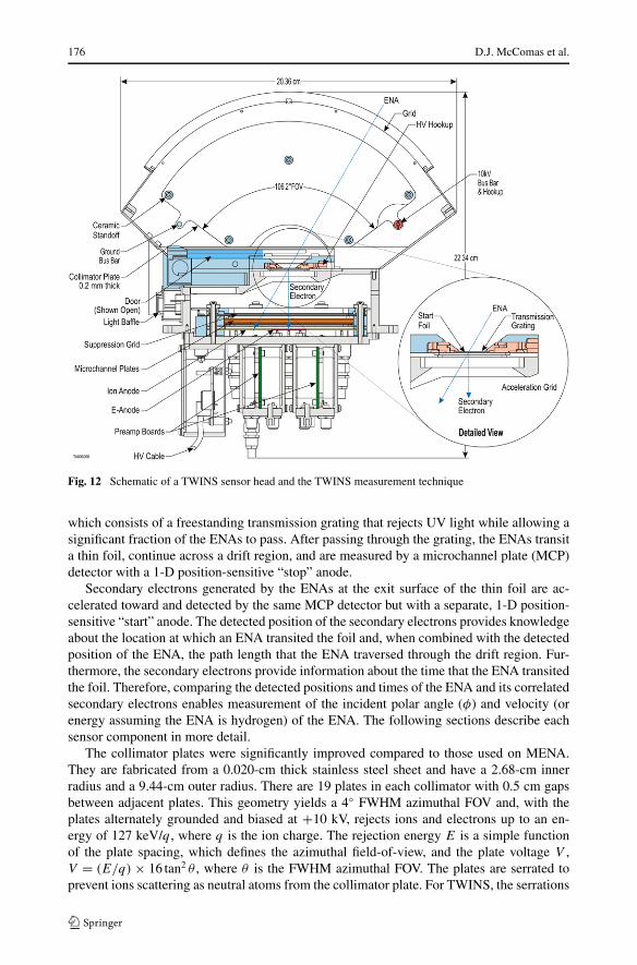
Fig. 12 Schematic of a TWINS sensor head and the TWINS measurement technique
which consists of a freestanding transmission grating that rejects UV light while allowing asignificant fraction of the ENAs to pass. After passing through the grating, the ENAs transita thin foil, continue across a drift region, and are measured by a microchannel plate (MCP)detector with a 1-D position-sensitive “stop” anode.
Secondary electrons generated by the ENAs at the exit surface of the thin foil are ac-celerated toward and detected by the same MCP detector but with a separate, 1-D position-sensitive “start” anode. The detected position of the secondary electrons provides knowledgeabout the location at which an ENA transited the foil and, when combined with the detectedposition of the ENA, the path length that the ENA traversed through the drift region. Fur-thermore, the secondary electrons provide information about the time that the ENA transitedthe foil. Therefore, comparing the detected positions and times of the ENA and its correlatedsecondary electrons enables measurement of the incident polar angle (φ) and velocity (orenergy assuming the ENA is hydrogen) of the ENA. The following sections describe eachsensor component in more detail.
The collimator plates were significantly improved compared to those used on MENA.They are fabricated from a 0.020-cm thick stainless steel sheet and have a 2.68-cm innerradius and a 9.44-cm outer radius. There are 19 plates in each collimator with 0.5 cm gapsbetween adjacent plates. This geometry yields a 4◦ FWHM azimuthal FOV and, with theplates alternately grounded and biased at +10 kV, rejects ions and electrons up to an en-ergy of 127 keV/q , where q is the ion charge. The rejection energy E is a simple functionof the plate spacing, which defines the azimuthal field-of-view, and the plate voltage V ,V = (E/q) × 16 tan2 θ , where θ is the FWHM azimuthal FOV. The plates are serrated toprevent ions scattering as neutral atoms from the collimator plate. For TWINS, the serrations

The Two Wide-angle Imaging Neutral-atom Spectrometers (TWINS) 177
are cylindrical with a radius of 50 µm and a period of 100 µm (Fig. 13). Laboratory mea-surements comparing these serrated plates with Ebonol-C, a highly dendritic surface coatingused on the MENA collimator plates, showed that these serrations reduced scattering of in-cident 20 keV H+ by a factor of 25–50 better than Ebonol-C when ions were incident ina plane perpendicular to the serration channels (the factor was still 2.5–3 even when ionswere incident in a plane parallel to the serration channels). Additionally, the serrated surfacereduced UV (1216 Å) reflection by a factor of 3 better than the Ebonol-C when the UV wasincident in a plane that was perpendicular to the serration channels.
Figure 14 shows the measured suppression of 20 keV H+ through the TWINS collimatorplates. The experiment was performed at 4 × 10⁻⁸ Torr. For this test, the incident ion beam,which contains some fraction of neutral particles, first transited an electrostatic chicane. Thisstructure consists of two sequential but opposite deflections so that the ion beam exiting thechicane is parallel to the incident beam but displaced several cm, thus stopping the neutralcomponent of the beam in the chicane. The ions continued 50 cm to the collimator, and ionsthat transited the collimator were measured by an MCP detector. The interpretation of thedata in Fig. 14 depends on the neutralization of ions over the 50 cm between the chicane andthe collimator. Using a neutralization cross section of 4×10⁻¹⁶ cm2 (Stier and Barnett 1956;
Fig. 13 Serrations in theTWINS stainless steel collimatorplates. The radius of a serrationchannel was 50 µm, and thechannel period was 100 µm
Fig. 14 Measured iontransmission through the TWINScollimator. Because ions in theincident beam can becomeneutral by charge-exchange withambient gas molecules in thevacuum chamber, these numbersrepresent an upper bound for iontransmission through thecollimator

178 D.J. McComas et al.
Lindsay and Stebbings 2005), the probability of neutralization of ions in the incident beam is∼3×10⁻⁵, which is approximately 1/3 of the measured transmission for collimator voltagesof 6–10 kV. Additionally, because of dynamic range limitations and non-zero backgroundcount rates in the MCP detector, both of which contribute to background and error in themeasurements of Fig. 14, these measurements represent an upper limit to the transmissionof ions through the collimator.
2.3.1 Transmission Gratings
The freestanding transmission gratings act as lossy waveguides to block UV light from en-tering the detector section while allowing ENAs to pass through with transmission TION.A freestanding transmission grating, illustrated in Fig. 15, consists of a series of gold grat-ing bars fabricated using holographic X-ray lithography; the bars are 460 nm thick and havea nominal period of 200 nm with a 45 nm slot width (gap). These bars sit on top of a Nisupport grid that consists of two integrated coplanar structures, both 1.12 µm thick; a largertriangular grid structure with legs ∼400 µm long and 12 µm wide; and fine support bars3.00 µm wide, separated by 1.02 µm, and perpendicular to the gold grating bars. Figure 16shows a picture of a grating from the Flight Model (FM) 1 Toward sensor head. The actualgrating bars run vertically but are too fine to be seen in this image. The triangular Ni supportstructure for the grating bars is clearly visible.
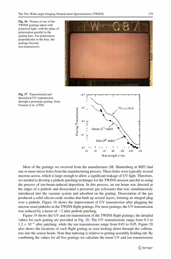
Considerable experimental and theoretical work has been performed to characterizethe UV and ENA transmission properties of the gratings (Gruntman 1995; 1997; Scimeet al. 1995). Figure 17 shows experimental and theoretical results for a prototype grat-ing 494-nm thick with a 200-nm period and an inter-bar gap of 62 nm (Gruntman 1997;Funsten et al. 1998). The experimental data (symbols) are in excellent agreement with the-oretical simulations (dashed line) for zeroth-order diffraction. The solid line, which is atheoretical result with all diffraction orders included, is representative of the grating per-formance for unpolarized light and follows a general exponential decrease of transmittancewith increasing wavelength from 0.06 at 304 Å to 4 × 10⁻⁵ at 1216 Å. The TWINS flightgratings have UV-rejection properties that are significantly improved compared to this pro-totype grating.
Fig. 15 Geometry of theTWINS freestandingtransmission grating
The Two Wide-angle Imaging Neutral-atom Spectrometers (TWINS) 179
Fig. 16 Picture of one of theTWINS gratings taken withpolarized light, with the plane ofpolarization parallel to thegrating bars. For polarizationperpendicular to the bars, thegratings becomenon-transmissive
Fig. 17 Experimental andtheoretical UV transmissionthrough a prototype grating, fromFunsten et al. (1998)
Most of the gratings we received from the manufacturer (M. Shattenberg at MIT) hadone or more micro holes from the manufacturing process. These holes were typically severalmicrons across, which is large enough to allow a significant leakage of UV light. Therefore,we needed to develop a pinhole patching technique for the TWINS mission and did so usingthe process of ion-beam-induced deposition. In this process, an ion beam was directed atthe edges of a pinhole and dissociated a precursor gas (siloxane) that was simultaneouslyintroduced into the vacuum system and adsorbed on the grating. Dissociation of the gasproduced a solid silicon oxide residue that built up several layers, forming an integral plugover a pinhole. Figure 18 shows the improvement of UV transmission after plugging themicron-sized pinholes in the TWINS flight gratings. For most gratings, the UV transmissionwas reduced by a factor of ∼2 after pinhole patching.
Figure 19 shows the UV and ion transmission of the TWINS flight gratings; the detailedvalues for each grating are provided in Fig. 20. The UV transmissions range from 0.3 to1.2 × 10−5 after patching, while the ion transmissions range from 0.03 to 0.05. Figure 20also shows the locations of each flight grating as seen looking down through the collima-tors into the sensor heads. Note that indexing is relative to grating assembly holding tab. Bycombining the values for all five gratings we calculate the mean UV and ion transmissions

180 D.J. McComas et al.
Fig. 18 UV (1216 Å)transmission before and afterpinhole plugging usingion-beam-induced deposition
for each TWINS sensor (right side of Fig. 20). In general, gratings with higher UV trans-mission also have higher ion transmission, preserving a relatively constant signal-to-noiseratio (e.g., ion-to-UV flux ratio). Because each of the four TWINS sensors has five gratingsand each grating is 1.71 × 1.00 cm, the average net-open aperture area for ENAs for eachsensor, based on the total grating area and the average ion transmission, is ∼0.37 cm2.
For IMAGE/MENA, the gratings were repeatedly exposed to the Sun for a few secondson each spacecraft rotation for certain seasons of the year. On TWINS, depending on thefinal orbits, the Sun could shine into the apertures at some actuator rotation phases during atleast one season. For TWINS, we were also concerned that the actuator could be parked inan orientation that would expose the gratings to direct illumination for a significant interval.While the operational plan is not to let this happen, we decided to carry out a combinedset of tests that covered both the repeated short time illumination and a long duration testrequired for both MENA and TWINS. We performed tests with flight-like gratings (poorergratings from the same batch being flown) and exposed them to a Xe arc-lamp to provide athermal load similar to that of the Sun (>1350 W/m2 at the gratings).
For the first test, a grating was exposed for 2 s every 10 s over 654,000 cycles. A cali-brated imaging infrared spectrometer was used to measure the increase in the temperatureacross the grating. At the end of a 2 s exposure, the average grating temperature was 23◦Cand the maximum temperature, which occurred at the grating center, was ∼25◦C. The ENAand UV transmissions were measured before the thermal testing, after the testing, and every∼100,000 cycles during the testing. For the second test, five gratings were exposed to thearc-lamp continuously for 20 minutes. Spatial temperature distributions across each gratingwere similar to that observed in the first test. The equilibrium temperature difference be-tween the hottest points at the centers of the grating and the grating frames, which acted asheat sinks, was ∼50◦C. This agreed well with a thermal model of the grating, which de-rived an expected temperature difference of 45◦C. Finally, we ran a third test over another136,000 cycles using a patched grating. In all three tests, no measurable change of UV orENA transmission was observed, and no visible changes such as wrinkling were noted. Thisextensive testing clearly demonstrates how robust our gratings are against solar illuminationand heating.

The Two Wide-angle Imaging Neutral-atom Spectrometers (TWINS) 181
Fig. 19 Measured UV and5 keV H+ transmission for theTWINS flight gratings
Fig. 20 Locations and measured transmission values for all 20 flight gratings

182 D.J. McComas et al.
Figure 21 shows the intrinsic angular response of a grating to a narrow ion beam in-cident at the center of a grating. The azimuthal response (top panel) distribution shows afull width at half maximum of approximately 18◦, which is substantially wider than the 4◦
azimuthal response provided by the collimator. The polar response (bottom panel) shows abroad response function; the relative transmission decreases at higher polar angles but doesnot fall below a value of 0.5 over the range of ±50◦. As the grating is tilted relative to thebeam, the beam traverses a longer distance through the grating in a direction parallel tothe grating bars. Therefore, this response is not just the cosine effect resulting from a tiltedflat aperture, but rather due to the collimation effect of traversing a longer distance through
Fig. 21 The intrinsic angularresponse of a grating to a narrowion beam incident at the center ofa grating. The azimuthal response(top panel) distribution shows afull width at half maximum ofapproximately 18◦, which issubstantially wider than the 4◦azimuthal response of thecollimator. Finally, although thegold gratings do not collimate inthe polar angle direction, a littlecollimation is provided by thefine nickel support bars

The Two Wide-angle Imaging Neutral-atom Spectrometers (TWINS) 183
the grating bars. The decrease in the transmission results from the slight irregularities inthe linearity of individual grating bars and in the parallelism between adjacent bars. Thepolar angle measurement can have significant error at high polar angles because of the sen-sitivity of transmission due to the relative alignment of the incident ion beam direction andthe direction of the grating bars. This effect probably causes some observed asymmetry ofpolar-angle distribution.
2.3.2 Carbon Foil
Ultra-thin carbon foils (∼50 Å thick), mounted on highly transmissive grids, have been usedsuccessfully in a wide variety of space missions (McComas et al. 2004). For TWINS, as forMENA, these foils were mounted directly on the backs of the gratings. The forward sec-ondary electron yield of H+ transiting thin-carbon foils has been measured to range from2.1 to 4.5 over an energy range of 10–90 keV (Ritzau and Baragiola 1998). Because hydro-gen reaches charge-state equilibrium before it exits the foil, the forward secondary electronyield for H◦ should equal that of H+. The grating (and therefore foil) is biased to −2 kVso that secondary electrons are accelerated toward a 70 line-per-inch grounded accelerationgrid located behind the grating. Therefore, secondary electrons are quickly accelerated to-ward the “start” anode region of the MCP detector. This acceleration enables the detectedposition of the secondary electrons on the detector to accurately represent the locations atwhich ENAs transited the foil. The ENA trajectory measurements are obtained using the de-tected positions of an ENA and its associated secondary electrons. The TOF measurementis derived from the time difference between detection of the secondary electrons, which aredetected first, and the ENA.
A down side of using start foils for timing is that the incident particles undergo energystraggling and angle scattering as they pass though the foils. The magnitudes of these effectsare functions of 1) the foil properties, 2) the foil thickness, and 3) the incident energy andspecies of the particle passing though the foil (Funsten et al. 1993; Allegrini et al. 2006).For particles arriving at the carbon foils with the same incident angle and energy, the moremassive particles experience larger energy loss and angular scatting as they pass through.Because of this, the TWINS instrument will make higher resolution measurements of thehydrogen ENAs than the oxygen ENAs. The magnitude of the energy straggling and angularscattering is reduced for all species as the foil thickness is reduced. To keep the energystraggling and angular scattering to a minimum, we are using carbon foils as thin as hasbeen reliably flown to date (nominal thickness ∼0.5 µg/cm2) (McComas et al. 2004).
2.3.3 MCP Detector
ENAs and associated secondary electrons strike an 8 × 10-cm MCP detector in a Z-stack(3-plate) configuration. The MCPs are standard Hamamatsu plates with a 40:1 length-to-diameter channel ratio. An electric field is applied at the entrance surface of the MCP detec-tor using a 70 line-per-inch suppression grid biased at −12 V and a +100 V bias on the frontof the MCP detector. This field increases both the detection efficiency of the MCP and thespatial imaging resolution (Funsten et al. 1996). In addition, the −12 V on the grid rejectssecondary electrons at thermal energies generated anywhere inside the sensors other thanthe carbon foils, which are accelerated by the −2 kV of bias voltage.

184 D.J. McComas et al.
2.3.4 Detector Anode
The ENA trajectory determination requires independent measurements of the one-dimen-sional (1-D) positions of the detected ENA and its associated secondary electrons. Further-more, the TOF determination requires independent measurements of the detection time ofthe secondary electron (start time) and that of the ENA (stop time). Therefore, the detectoranode is segmented into two regions: the Start region where secondary electrons from thestart foil are detected, and the Stop region where ENAs are detected. Each of these anoderegions provides 1-D position encoding via a capacitive-charge-division technique and isserviced by two charge-sensitive pre-amplifiers (A and B). The relative pulse amplitudes onthe A and B sides vary linearly with event position, allowing standard ratiometric positiondetermination.
The system supports independent position determination on the Start and Stop anode re-gions to a full-width spatial-resolution of 1 mm and TOF determination to a resolution of<20% for time ranges greater than approximately 7 ns, corresponding to the travel time ofa 100 keV H atom at normal incidence. The independent position determination provides1-D angular resolution of 3.8◦, considering the 3-cm flight path between the secondary elec-tron emission foil and the MCP input face. The intrinsic energy resolution of the imager is�E/E = 2(�t/t) = 0.4 based on the 20% time resolution. This does not include the energystraggling of the ENAs in the secondary electron emission foil, which must be included forunderstanding the energy dependence of the instrument response.
2.3.5 Charge Amplifiers
The Charge Amplifiers are a discrete, high-speed design with two inputs, A and B , and twooutputs, A and the sum A + B . This is convenient for the downstream electronics becausethe sum, A + B , is independent of location on the anode. This quantity is useful for TOFmeasurement and pulse height analysis, while the ratio of A/(A + B) yields the locationof the event on the anode and thus provides the imaging information. There are separateCharge Amplifiers for the Start and the Stop sections of each Sensor Head.
The charge from each A and B wedge input is received through a protection networkthat includes a blocking capacitor, a current limiting resistor, and back-to-back diodes. Thecharge to voltage conversion is performed by a JFET transistor followed by a pair of RFtransistors for current gain with feedback through a capacitor. This is followed by shapingnetworks which provide a bipolar pulse for A and a bipolar pulse for the sum of A+B . Theoutput stage is an operational amplifier with high gain in the narrow frequency bandwidthof the bipolar pulse and the ability to drive the coaxial output cable. The Charge Amplifiersare adjusted to provide a gain of 0.15 V/pC. The dynamic range is from the noise floor of0.6 mV rms to a maximum output without any distortion of the bipolar pulse of 7 V. Thebipolar pulse is shaped to provide a zero-cross 180 ns after the input MCP charge dump. Thistuned circuit, like a pendulum, maintains an accurate zero crossing time that is independentof the pulse amplitude. In practice the variation is very small (less than ±1 ns) and providesa simple way to determine TOF using a zero cross detection circuit.
2.4 Lyman-α Detector (LAD)
Inversion of the TWINS line-of-sight integrated ENA measurements requires knowledge ofthe geocoronal neutral density distribution. This is because the hydrogen geocorona pro-duces the ENAs from local ions via charge-exchange. For TWINS, we have directly ad-dressed this need by including a dual-headed Lyman-α sensor, called the TWINS-LAD.

The Two Wide-angle Imaging Neutral-atom Spectrometers (TWINS) 185
These detectors provide line-of-sight integrated Lyman-α resonance emission intensitiesalong two central lines of sight within the TWINS ENA FOVs. With the help of a numericalinversion routine (Zoennchen 2006) we obtain actual hydrogen densities needed for detailedanalysis of the ENA signals.
The inversion is relatively straightforward as long as the lines-of-sight of the TWINS-LAD detectors are fully embedded in the optically thin part of the geocorona, since inthese regions all Lyman-α radiation source volumes are illuminated by the same solarLyman-α input intensity. In this case, source strengths for local Lyman-α resonance emis-sion are simply proportional to the local hydrogen density. The requirement of optical thinconditions is fulfilled for almost all of the lines-of-sight observed by TWINS. The primegoals of the inversion of TWINS-LAD data are 1) derivation of the actual global hydrogendensity distribution with a presently unachieved resolution in altitude, latitude and longi-tude, and 2) optimization of theoretical hydrogen geocorona models including represen-tations for the hydrogen geo-tail and the H-atom satellite exosphere (Chamberlain 1963;Chamberlain and Hunten 1987). The LAD sensor, science, and inversion techniques weredescribed briefly by Nass et al. (2006).
The LAD is mounted on top of the DPU and consists of two identical Lyman-α detectors,which are arranged in a plane parallel to the two TWINS sensor heads and inclined by ±40◦
to the actuator’s rotation axis. Figure 22 shows the basic measurement principle of the LADdetectors: the Lyman-α radiation enters a collimator (Baffle) through an optical interferencefilter (BP-Filter) centered at 122 nm with a width of 10 nm FWHM. The collimator is madeof blackened aluminum honeycomb material, with a length of 25.4 mm and a cell pitchof 1.53 mm, defining a circular FOV of approximately 4◦. The Lyman-α radiation is thendetected by a CEM with an attached amplifier/discriminator circuit. The output pulses of
Fig. 22 Functional block diagram of the LAD sensors

186 D.J. McComas et al.
the discriminator are measured by a digital pulse counter with the frequency of these pulsesbeing proportional to the instantaneous Lyman-α intensity.
The LAD sensors were designed by the Institute for Astrophysics and Space Research,University of Bonn. The company von Hoerner & Sulger GmbH (Schwetzingen, Ger-many) was the main contractor for the LAD and did all of its development, manufactur-ing, and qualification. All LAD sensors were calibrated at the Berlin Electron Synchrotron(BESSY II). This facility was operated at very low currents yielding Lyman-α radiation withan intensity covering the range of expected geo-coronal values.
During the mission the actuator rotates the instrument in a windshield-wiper motion backand forth through 180◦ with a rotation speed of 3◦ per second. Since the two sensors aresymmetrically oriented about the rotation axis, a full circle is mapped each rotation. Thecounters are read out each 0.67 seconds (corresponding to 2◦ at the nominal 3◦ s−1 TWArotation rate), which yields a spatial resolution of approximately 4◦ × 6◦. At the two endpoints (0◦ and 180◦) the detectors alternately view the same region of space, thus enablinga near continuous check of their relative calibration.
The total Lyman-α line-of-sight intensity is given by
I = IBG + 1
4π
∫n(s)g(s)ds (2)
with the interplanetary Lyman-α background intensity IBG, the neutral H density profilen(s), and g(s), the resonance scattering rate, along the line of sight. The R.R. Hodges-model(Hodges 1994), which describes the terrestrial hydrogen exosphere up to ∼60,000 km fromthe geo-center, based on a third-order spherical harmonic expansion, was initially used. Toreduce the large number (∼200) of free Hodges-parameters, a “Parameterized ExosphericModel (PEM)” was derived by fitting the r-dependences of the expansion coefficients givenby Hodges in a set of functions. As a result, the PEM needs only 30 parameters while stillproviding good agreement with the densities of the Hodges-model for different solar F10.7
cm fluxes between 80–230 × 10−22 W m−2 Hz−1.The solar radiation input of the Lyman-α line-centered flux is derivable from ter-
restrial measurements of the F10.7 cm flux or the equivalence-width of the solar He1083-absorption line. Depending on what other assets are available over the TWINS mission,we will also attempt to use direct solar Lyman-α observations as input. For example, whileSOHO is still functioning, the Lyman-α line-centered flux will be directly available fromUARS/SOLSTICE.
To separate and eliminate the interplanetary Lyman-α background radiation (∼102 R)from the geocoronal radiation (∼103–104 R), Local Interstellar Medium (LISM) Lyman-αintensity-maps were calculated for background subtraction using the hydrogen distributionmodel of the solar system from Bzowski et al. (2002, 2003). Stellar Lyman-α emissions, forexample from young, bright OB-stars, can be easily eliminated by their typical peak-profilewithin the LAD scans. In addition, those stellar peaks could also be used to provide anabsolute “in flight” calibration of the LAD detectors. Based on the PEM and TWINS orbitalgeometry, we produced a simulated set of line-of-sight, Lyman-α data. These pseudo-datahave been successfully used to reconstruct the original PEM by fitting over as little as one-half of an orbit (see Fig. 23).
The coverage of the geocorona increases over progressive TWINS orbits producing com-plete maps each year. Availability of Lyman-α data from different parts of the geocoronawill increase the quality of the fitted geocoronal hydrogen model. Additionally, the relationbetween the geocoronal hydrogen distribution and the solar F10.7 flux will be determined.Together, these procedures will allow us to produce a 3-D time-dependent geocoronal hy-drogen density model for the magnetospheric regions observed by TWINS.

The Two Wide-angle Imaging Neutral-atom Spectrometers (TWINS) 187
Fig. 23 Reconstructed test hydrogen densities (red) fitted from the Lyman-α intensities of one-half of anorbit are in good agreement with the PEM H-densities (black). Contours are labeled in atoms/cm3
2.5 DPU and Electronics
2.5.1 Data Processing Unit (DPU)
The data processing unit (DPU) is a completely new design for TWINS, owing to the dif-ferences between the IMAGE and TWINS spacecraft interfaces and the need to incorporatea rotational actuator. The DPU provides the spacecraft command and telemetry interface toTWINS and controls the ENA sensors, LAD, and TWA operations. The DPU is comprisedof two boards, the data processor (DP) and interface (IO) boards, designed specifically forthe TWINS instrument to optimize for low power, low mass, and fast telemetry process-ing. Figure 24 is a block diagram of the DP board. The DP board is an 80C186-based,single-board computer, running at 12 MHz with 256 kbytes of static RAM and 64 kbytes ofprogram ROM. An additional 512 kbytes of EEPROM is provided for storing code revisionsand lookup tables. An Actel RH1280 FPGA provides the glue logic for the microprocessoras well as a custom co-processing machine for constructing neutral-atom images from theFront End Electronics (FEE) raw data. The DP board also contains the 1553 interface elec-tronics, which use UTMC’s remote-terminal chipset and a dedicated 64 kbytes of RAM forthe telemetry and command buffering.
A block diagram of the IO board is shown in Fig. 25. The IO board provides the electricalinterfaces between the DP board and the other TWINS subsystems. It controls the rotation ofthe actuator using an 80C32 micro-controller chip. This dual-processor design (i.e., 80C186for telemetry, and 80C32 for rotation) keeps the timing of the telemetry tasks insulated fromthe critical timing of the actuator rotation.
The IO board also provides counters for the Lyman-α detector and controls the deploy-ment of the ENA doors and TWA Marmon clamp. A 12-bit A/D converter is provided fordigitization of all TWINS analog housekeeping.
2.5.2 Front-End Electronics (FEE)
The FEE services the two ENA sensor heads and provides all of the analog and digitalprocessing to measure the angle and speed of each incoming neutral atom and to estimate

188 D.J. McComas et al.
Fig. 24 Data Processor board block diagram
its species based on the amplitude of the MCP pulses. The anode and charge amplifierswere described in Sects. 2.3.4 and 2.3.5. Together they serve to create the analog signalsSTART_A, START_SUM, STOP_A, and STOP_SUM which are then processed by the TOFboard (FEE_TOF) and the pulse height analysis board (FEE_PHA). Each sensor head isserviced by a pair of FEE_TOF/FEE_PHA boards which convert the analog pulses fromthe sensor into digital values for the position and pulse height of the start and stop signals.A block diagram of the Front End Electronics is provided in Fig. 26.
The FEE Control board (FEE_CTL) provides an interface to the front end electronics forthe software on the DPU board. The difference in arrival time between the START_SUMand the STOP_SUM signals is used to measure the TOF. Until a pulse breaks the low leveldiscriminator (LLD) of the START_SUM signal, the FEE_TOF and FEE_PHA are held inreset. Once the Start signal exceeds the LLD, a high speed, low dispersion comparator isenabled that looks for the transition of the bipolar pulse back through ground. Once thissignal is received, a constant current source is used to begin charging a capacitor. A similarcircuit is used to process the STOP_SUM signal. The voltage on the capacitor is subse-quently digitized by an A/D Converter and then cleared. A 15 ns time delay is insertedinto the STOP_SUM signal processing to eliminate non-linearity for very short TOFs. TheFEE_TOF measures TOF from 5 ns to 330 ns with a nominal resolution of 1.4 ns/LSB. Aftera valid ENA event has been processed, the 8-bit digital value for the TOF is passed to theFEE_CTL board.
The FEE_TOF employs several strategies to eliminate erroneous measurements. Fixed-value upper level discriminators are used to make sure that the START_SUM andSTOP_SUM signals have not exceeded their linear range. The lower level discriminators

The Two Wide-angle Imaging Neutral-atom Spectrometers (TWINS) 189
Fig. 25 IO board block diagram
can be set through software to adapt to any changes in the noise floor level. Comparatorscheck the analog value of the TOF signal to see if it is too short or too long to be a validENA. A flip-flop is used to check if a second Start signal has arrived before a valid Stopsignal has arrived. All of these conditions are flagged as errors, recorded, and then the FEEis quickly reset to be ready for the next ENA without wasting time on the relatively long A/Dconversion process for an invalid event. This minimizes the dead-time spent processing UVphotons or other false events. The raw outputs of the Start and Stop LLDs bypass the controllogic and are accumulated by high-speed counters on the FEE_CTL board to monitor thestart and stop count rates on the MCP for detector safety.
The position of the start and stop signals on the anode are used to determine the 1-Dincidence angle of the ENA. The amplitude of the start and stop signals are also used in thealgorithm that estimates the species of the ENA. Once signals for a valid event have beencaptured, no further input can corrupt the values while the analog ratio circuits, A/(A + B),settles and the A/D converters complete their conversions (20 µs). After the conversion iscomplete for a valid ENA, latches on the FEE_PHA now hold 8-bit digital values for theSTART_POSITION, START_HEIGHT, STOP_POSITION, and STOP_HEIGHT.
The FEE_PHA uses comparators to ensure that the analog values of ratios are withinthe minimum and maximum ratios prescribed by the geometry of the anode before an A/Dconversion cycle is initiated. If the ratios are out of bounds, the error, or any error generatedby the FEE_TOF, is captured by the FEE_CTL board and the FEE is promptly reset.

190 D.J. McComas et al.
Fig. 26 Front end electronics block diagram
The ENA sensor heads use a collimator voltage that can be commanded up to +10 kVto sweep out ions, a MCP voltage commendable up to +4 kV to power the detectors, and a−2 kV foil bias supply to provide acceleration of the secondary electrons from the carbonfoil which are used to generate the start signals. A separate HVPS board provides thesevoltages to each sensor head.
The +10 kV collimator supply is capable of producing full voltage while providing upto 12 µA of current. The +4 kV MCP supply is capable of producing full voltage whileproviding up to 54 µA of current. The −2 kV foil supply, which can produce up to 35 µAis actually two supplies, one driven off of the collimator supply and one driven off of theMCP supply, which are diode OR-ed together. The outputs have “zap traps” to provide aprotective current path to chassis in the event of a high voltage breakdown. The suppliescan safely drive a dead short indefinitely and recover with a small overshoot (<10%) if theshort is removed. Conservative high voltage spacing is used throughout the design, but foran extra measure of safety the HVPS and its multiplier chains have a conformal coating ofparylene which has a high dielectric strength.
The FEE_CTL board provides the interface to the FEE for the software running on theDPU. These functions include: high voltage enable, high voltage level commands, settingthe LLD for the FEE_TOF board, real-time processing of events from the FEE_TOF andFEE_PHA boards, buffering the valid event data in memory, counting occurrences of thevarious types of errors, counting the total starts, stops, & valid events, generating test pulserpatterns, and monitoring the inputs from the external Safe/Arm connector. A block diagramof the FEE_CTL board is shown in Fig. 27.

The Two Wide-angle Imaging Neutral-atom Spectrometers (TWINS) 191
Fig. 27 FEE_CTL block diagram
2.5.3 Operating Modes
There is one principal science mode for the TWINS instrument: Dynamic Imaging Mode. Inthis mode, neutral-atom raw events and images are collected on 4◦ azimuthal sectors over the180◦ constant-velocity scan range. Although the neutral-atom telemetry is collected on 4◦sectors, the raw-event data is resolved further into 1◦ slices and tagged as such in telemetry.Another similar mode on TWINS is called Dynamic Test Mode, which differs only in thatthe telemetry is allocated to raw events and no neutral-atom image data is transmitted. Bothof these modes are position synchronous. Two other modes: Static Imaging and Static Test,are time-synchronized. These modes produce the same telemetry as the dynamic modes,but on time boundaries of 1.333 seconds, and were included primarily to support sensorcalibration when the actuator was not attached to the TWINS instrument.
The other TWINS modes are for engineering operations only and produce no sciencedata. Memory uploads are supported in a maintenance mode, whereby the DPU operatessolely from hard-coded PROM while the EEPROM data and SRAM data are being modified.Another mode, called Engineering Mode, provides only housekeeping data and is used fordeployments and other engineering diagnostics.
2.5.4 On-board Neutral-Atom Image Processing
FEE raw event data, consisting of digitized pulse heights and positions from the start andstop anodes in addition to TOF data, are input to a sequence of lookup tables encoded in anFPGA. These tables classify up to 25,000 events per second into one of 3,072 pixels. Five

192 D.J. McComas et al.
Fig. 28 Neutral-atom image formation flow (numbers in parentheses are the number of bits assigned to thelookup table address)
Fig. 29 TWA mounted on thetilt bracket in latchedconfiguration
lookup table cycles are performed as shown in Fig. 28 to construct a scalar array of polarangle, species, and energy pixels. Each pixel is initially 16-bits, which is compressed to 8bits for transmission.
2.6 TWINS Actuator (TWA)
In order to provide broad magnetospheric viewing from the 3-axis stabilized TWINS space-craft, we included a TWINS actuator (TWA) (Fig. 29) under the Instrument Baseplate be-

The Two Wide-angle Imaging Neutral-atom Spectrometers (TWINS) 193
tween the TWINS interface Plate and Tilt Bracket (see Fig. 8). The TWA rotates back andforth in a windshield-wiper motion about an axis that is pointed ∼10◦ from nadir. The TWAactuates over 180◦ in 60 s at a constant rate of 3◦ s−1 and then takes 22 s to slow, stop, andreaccelerate to the nominal rotational rate in the opposite direction. Thus, the TWINS entireFOV is mapped out over 60 s each 82 s. Control of the actuator is provided by the DPU.
The TWA design is based on the CAPS/ACT actuator currently flying on Cassini (Yliko-rpi et al. 1995). The TWA has a minimum operational lifetime of 4 years and was designedto minimize mechanical disturbances to the spacecraft. Starting with the CAPS actuatordesign, we made only the changes necessary to accommodate differing TWINS functionalrequirements, differences between the Cassini and host spacecraft, and upgrades of severalparts. These design changes are provided in Table 3.
The main TWA interior parts are shown in Fig. 30. We describe the TWA in three func-tional parts: the motor unit, launch latch and electronics subsystems.
Table 3 TWA design changesfrom Cassini/CAPS design Actuator component Design change
Launch latch Increased preload
Grounding pin Added
Purge feedthrough Removed
Potentiometer Changed supplier
Cable wrap Changed supplier
Rotor housing Removed connector ports
Stator housing Changed connector ports
Scanning range Relocated
Clamp ring Relocated
Mumetal magnetic shields Removed
Bearings Changed from copper beryllium to steel
EMI mitigation copper taping Added
Velocity feedback Used as analog signal
DPU interface Simplified
Fig. 30 Main components of the TWA

194 D.J. McComas et al.
Fig. 31 Cross section of the TWA motor unit
2.6.1 Motor Unit
The motor unit (Fig. 31) turns the TWA rotor and the TWINS instrument nominally ±99◦around its center position. The angular position of TWINS is measured with a resistivepotentiometer, which is mounted between the motor housing and a non-rotating flange. Thelinearity of this high-precision monitor is accurate to ±0.1◦. Two additional known positionsfor the motor are provided by limit switches that produce signals at ±106◦ in case of over-rotation. Hard stops are located at ±110◦. A sliding contact in the bore reduces the bondingresistance between the rotor and stator to <5 m�. The motor unit is fully separable fromthe TWA structure so that it could be built up and tested as a separate subsystem.
The hybrid stepper motor is the same used in the SWAN (Solar Wind ANisotropy) in-strument in the SOHO spacecraft (Bertaux et al. 1995). The SAGEM motor provides 300 mNm torque with 65 mA current.
The non-separable angular contact ball bearings are manufactured of 440C steel. Thebearings are mounted in X-configuration where they are pushed into the seats by an axialpreload provided by a flexible flange. The bearings are lubricated with ion-plated lead asrecommended and processed by the European Space Tribology Laboratory (ESTL). Greatcare was exercised to guarantee sufficient bearing preload under all circumstances, becauselubricant and rolling surfaces can be easily damaged if the balls skid instead of roll alongthe ball track.
To fully analyze the bearing assembly, ESTL used special in-house software that cal-culates values for preload and friction torque for specified bearing-seat axial stiffness andtemperature differences between the housing and the shaft. The software also provided es-timates for the steady mean torque as a function of preload. With the aid of these simula-tions, we determined the required bearing preload and housing stiffness: 50 N preload and0.5 µm/N stiffness to produce a mean friction torque of 0.002 N m over a tolerable temper-ature difference of 15◦C between the bearing rings.
The stiffness of the preloading flange is measured separately in a jig. Bearing preloadis adjusted by an adjusting ring placed between the bearing inner rings. The thickness ofthe ring defines the distance between the bearing inner rings, while the outer rings arepressed towards each other by the housing. Bearing preload is determined by measuringthe height of the motor housing with and without the bearings. The bearing axial-static limitload is 1030 N and axial-dynamic limit load is 290 N. ESTL measurements of four pairs ofTWINS bearings in vacuum with 50 N preload yielded mean friction torques from 0.001 to0.002 N m validating the simulated values.

The Two Wide-angle Imaging Neutral-atom Spectrometers (TWINS) 195
Fig. 32 TWA Launch Latch assembly
2.6.2 Launch Latch
Because the bearings cannot carry any launch loads for the TWINS instrument, all loadsare transferred through the TWA structure using the Marman-Clamp (or V-Band Clamp)latching device (Fig. 32).
Operating the latch requires a 2-mm axial separation between the rotor and stator, whichis provided by a flexible mounting between the motor shaft and the TWA stator. The steppermotor stator (the part with windings) is rigidly mounted to the TWA rotor. When latched therotor and motor assembly are displaced 2 mm. Compression springs keep the upper bearingpreloaded against vibration loads during spacecraft launch. When unlatched the rotor andassociated parts move back into position. With this design the compression springs do notproduce any loads on the bearings or motor assembly in the released state.
The structure of the latch ring is significantly different from most common Marman-clamps where several small clamps are pressed with the aid of a tensioned steel band. ForTWINS we use a tensioned circular clamp because the latch ring radius was limited to92 mm, which is small relative to external loads. Thus, it was necessary to utilize the entirecircumference for clamping. When unlatched, the latch ring extends 2-mm larger in diameterthan the TWA lips, which require 31-mm expansion in circumference. The expanded ringis pulled by tension springs to rest against the shelves, guaranteeing that the ring can nottouch or interfere with the TWA stator. The ring is machined from an aluminum plate tomatch its larger diameter in a relaxed state, and during latching it bends around the TWAstructure. The inside profile is machined to be circular in the latched position while theoutside profile is made to be circular in the relaxed state. The latch ring is tensioned byturning the tightening screw with a pre-determined torque. The latch ring and its lockingmechanism are enclosed in a cage with tie down points for the MLI.

196 D.J. McComas et al.
Another unusual aspect of the clamp ring is the locking mechanism. The clamp is fullyrelatchable and operated by a wax thermal actuator (WTA). The WTA operates a latch-actuating mechanism (LAM) by pushing a small hook forward and releasing a locking pin ona lever. The lever is a part of an over-center mechanism used to reduce a 6500 N tension forceof the band down to 65 N at the locking pin. The movement of the hook is perpendicular toexternal forces at the pin, therefore it cannot open by itself. The latch-opening torque is verysmall while the tensioning force on the pivot and lever shaft remains at 6500 N. Such a largeforce can cause a larger frictional torque than appropriate for sliding bearing or bushings.Therefore, we used needle bearings with a measured coefficient rolling friction of 0.003.This solution provided a safety margin of 15 for bearing friction.
2.6.3 Electronics
A functional block diagram of the TWA electronics is shown in Fig. 33. The TWA uses a90-pole two-phase, bipolar direct-drive synchronous motor with a full step angle of 1◦. Themotor is driven in synchronous mode. The required phased voltages are generated from look-up tables using a dedicated microcontroller in the DPU. Appropriate combinations of valuesin the look up table produce the desired acceleration, direction and speed, and decelerationof the TWA by sending two 8-bit data words to the TWA, one for each phase of the motor.
The DPU interface decodes the commands sent by the TWINS DPU and generates apair of data words and polarity signals, one set for each phase. The motor drivers consistof two step-down Buck converters and two H-bridges for polarity switching. The step-downconverters generate voltages up to 15 V, which are fed to the motor windings. By settingthe H-switches, bipolar winding voltages of −15 to +15 V can be generated. The polarity
Fig. 33 Functional block diagram of the TWA electronics

The Two Wide-angle Imaging Neutral-atom Spectrometers (TWINS) 197
of the phase voltages is switched when the converter output voltage is zero. Depending onrequired torque and motor temperature, the DPU can control the maximum voltage between5 and 15 V.
The actual position of TWA is monitored from the position encoder. This signal is alsodifferentiated to produce a velocity monitor signal that is used to control the TWA rotationalspeed. An active control loop eliminates potential wobbling. Limit switch information isconnected to the databus in the DPU interface as a backup in case the TWA over rotates. Inaddition to the 8-bit data bus there are six control signals: two address lines, an enable (orstrobe) signal, power on reset signal, the stepping-synchronization pulse TWA_SYNC, anda 50-kHz clock for the pulse-width modulator (PWM) counters.
2.7 TWINS Environmental Sensor
In addition to the TWINS instruments, the TWINS S/C carry environmental monitors de-veloped under the auspices of the Aerospace Corporation’s Internal Research programs.The TWINS Environmental Sensor, Flight Model 1 (TWINS-ES FM1) consists of a classicthree-channel dosimeter (DOS) and an electrostatic plasma analyzer that serves as a surface-charging monitor (SCM); for FM2 the DOS is upgraded to a High Linear Energy Transfer(HiLET) detector. The TWINS-ES are provided for the TWINS host vehicle to gain an un-derstanding of the charged-particle environment and its variations over the mission as wellas to develop an understanding of the magnetospheric environment and dynamics observedin Molniya orbits. In addition, these observations will be of great value for interpreting theTWINS ENA observations. While not funded by the NASA TWINS program, these data areplanned to be made available to the community in parallel with the TWINS observationsat the TWINS web site. The TWINS-ES instruments will be described by Clemmons et al.(2008, manuscript in preparation).
The TWINS-ES is depicted in Fig. 34. It has a mass of 5.9 kg and dissipates 13 W. TheDOS domes are located as shown on a plate on the top of the instrument. The domes arealuminum hemispheres of thickness 0.30 mm, 1.2 mm, and 3.2 mm. A direct measurementof total dose is made. In addition, counts are accumulated in electron and proton channelsfor all three dosimeters. Thresholds for electrons (protons) are, respectively, approximately0.6 (8.5) MeV, 1.5 (16) MeV, and 3 (25) MeV. Rate and integrated counts for each channel
Fig. 34 The TWINS-ES FM1.The three DOS domes are seennear the top of the photograph.The aperture of the SCM is seennear the center, and the black boxat the bottom contains controland interface electronics
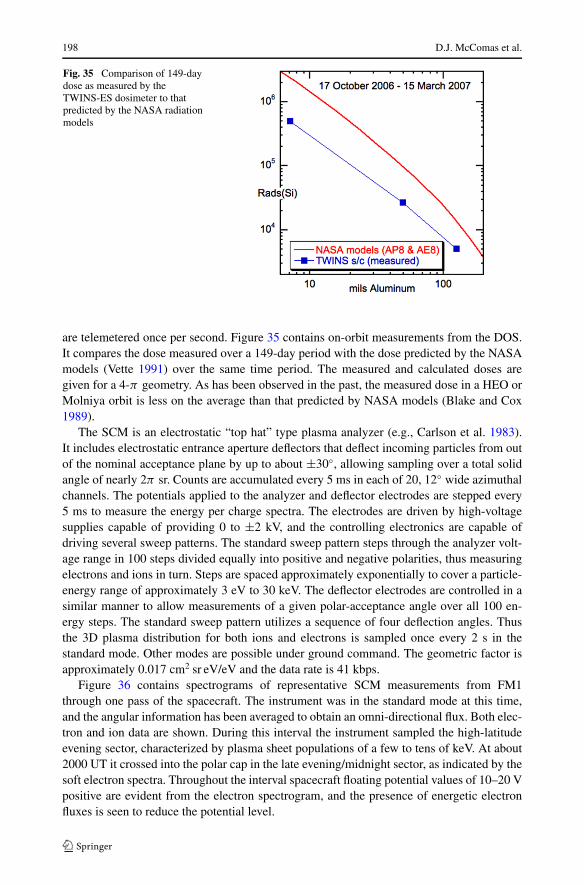
198 D.J. McComas et al.
Fig. 35 Comparison of 149-daydose as measured by theTWINS-ES dosimeter to thatpredicted by the NASA radiationmodels
are telemetered once per second. Figure 35 contains on-orbit measurements from the DOS.It compares the dose measured over a 149-day period with the dose predicted by the NASAmodels (Vette 1991) over the same time period. The measured and calculated doses aregiven for a 4-π geometry. As has been observed in the past, the measured dose in a HEO orMolniya orbit is less on the average than that predicted by NASA models (Blake and Cox1989).
The SCM is an electrostatic “top hat” type plasma analyzer (e.g., Carlson et al. 1983).It includes electrostatic entrance aperture deflectors that deflect incoming particles from outof the nominal acceptance plane by up to about ±30◦, allowing sampling over a total solidangle of nearly 2π sr. Counts are accumulated every 5 ms in each of 20, 12◦ wide azimuthalchannels. The potentials applied to the analyzer and deflector electrodes are stepped every5 ms to measure the energy per charge spectra. The electrodes are driven by high-voltagesupplies capable of providing 0 to ±2 kV, and the controlling electronics are capable ofdriving several sweep patterns. The standard sweep pattern steps through the analyzer volt-age range in 100 steps divided equally into positive and negative polarities, thus measuringelectrons and ions in turn. Steps are spaced approximately exponentially to cover a particle-energy range of approximately 3 eV to 30 keV. The deflector electrodes are controlled in asimilar manner to allow measurements of a given polar-acceptance angle over all 100 en-ergy steps. The standard sweep pattern utilizes a sequence of four deflection angles. Thusthe 3D plasma distribution for both ions and electrons is sampled once every 2 s in thestandard mode. Other modes are possible under ground command. The geometric factor isapproximately 0.017 cm2 sr eV/eV and the data rate is 41 kbps.
Figure 36 contains spectrograms of representative SCM measurements from FM1through one pass of the spacecraft. The instrument was in the standard mode at this time,and the angular information has been averaged to obtain an omni-directional flux. Both elec-tron and ion data are shown. During this interval the instrument sampled the high-latitudeevening sector, characterized by plasma sheet populations of a few to tens of keV. At about2000 UT it crossed into the polar cap in the late evening/midnight sector, as indicated by thesoft electron spectra. Throughout the interval spacecraft floating potential values of 10–20 Vpositive are evident from the electron spectrogram, and the presence of energetic electronfluxes is seen to reduce the potential level.

The Two Wide-angle Imaging Neutral-atom Spectrometers (TWINS) 199
Fig. 36 Omnidirectional fluxes of electrons (top panel) and ions (bottom panel) measured with the SCMover one satellite pass
3 Calibration and Instrument Performance
In addition to testing subsystems at their respective home institutions, the fully integratedTWINS instruments underwent extensive testing at the Southwest Research Institute Instru-ment Calibration Facility (see Appendix A). Each Flight Model underwent two calibrationsin this facility: 1) An extensive calibration prior to substituting engineering heads and envi-ronmental testing, and 2) an abridged test after reintegrating the flight heads after environ-mental testing.
Figure 37 shows a side view of the TWINS instrument. The TOWARD (AWAY) sensorhead is shown in orange (blue) and is designated as the head looking toward (or away)from the electronics box. Representative FOVs of ±50◦ are shown for both heads. Our signconvention designates negative angles as those coming from the electronics box (EBOX)side. The LAD (light blue) is notched to prevent any obstructions from the TOWARD sensorFOV. The notching in the LAD is independent of rotation angle because the DPU and LADsit on the actuator and thus rotate with the sensors.
Measurement of the responses of all sensor heads is critical for accurate generation ofENA images. Because the detailed performances of the heads differ slightly, we have per-formed extensive calibrations on each. Table 4 at the end of this section lists the performanceof each sensor head. Data from the four sensor heads are shown separately in the sectionsthat follow; the sensor head identifications are abbreviated by flight model and direction.For example, Flight Model 1 TOWARDS head is indicated as FM1T.
Figure 38 shows the TWINS FM 1 mounted in the calibration chamber in the config-uration used to calibrate the AWAY head (different mounting locations are used for theTOWARD and AWAY heads so that each sensor head is centered on the beam for its cal-ibration). The red “Remove Before Flight” covers and N2 purge line are still attached inthis photo. The sensor heads were kept under continuous N2 purge until the chamber doorwas closed and pump out was initiated. All interruptions in purge (e.g., during sensor headchange-out or just prior to closing the vacuum chamber door) are brief and logged. The

200 D.J. McComas et al.
Fig. 37 Side view of the TWINSinstrument. The TOWARD(AWAY) sensor head is shown inorange (blue). RepresentativeFOV of ±50◦ is shown for eachhead
Table 4 Sensor head performance
FM1A FM1T FM2A FM2T
Energy range perAMU [keV] @ 30◦
<1–112 <1–124 <1–114 <1–129
�E/E for H (3, 10,30, 50, 100a [keV]FWHM)
0.29, 0.49, 0.79,0.98, 1.32
0.38, 45, 0.52,0.57, 0.63
0.26, 0.34, 0.44,0.49, 0.57
0.27, 0.39, 0.56,0.66, 0.82
�E/E for O (10, 30,50, 100a [keV]FWHM)
0.43, 0.33, 0.30,0.26
0.43, 0.38, 0.36,0.33
0.54, 0.43, 0.38,0.33
0.50, 0.43, 0.40,0.36
Angular resolution(non-imaging,FWHM)
4.3◦ 4.3◦ 4.4◦ 4.5◦
Angular resolutionH > 10 keV(imaging, FWHM)
5.4◦ 4.8◦ 6.4◦ 6.3◦
Angular resolutionO > 10 keV(imaging, FWHM)
8.6◦ 7.9◦ 8.8◦ 9.9◦
FOVb ±55◦ ±55◦ ±55◦ ±55◦
Geometric factor(cm2 sr)
4.23 × 10⁻³ 4.51 × 10⁻³ 2.86 × 10⁻³ 2.74 × 10⁻³
MCP voltage [V](initial flight levels)
2700 2700 2500 2700
Collimator voltage[V] (initial flightlevels)
6500 6500 6500 6500
Largest TOF bytes map to ∼100 eV per AMU, however no data was taken below 1 keV hydrogen and 9 keVoxygen. Oxygen below 9 keV is detectable, but foil scattering effects blur imagesa100 keV data is extrapolated from lower energy calibration data
bField of view is quoted in the sensor frame. Appropriate mechanical offsets need to be applied to work inthe instrument frame
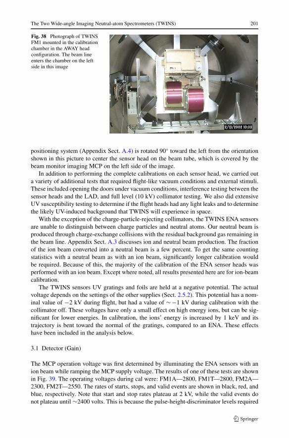
The Two Wide-angle Imaging Neutral-atom Spectrometers (TWINS) 201
Fig. 38 Photograph of TWINSFM1 mounted in the calibrationchamber in the AWAY headconfiguration. The beam lineenters the chamber on the leftside in this image
positioning system (Appendix Sect. A.4) is rotated 90◦ toward the left from the orientationshown in this picture to center the sensor head on the beam tube, which is covered by thebeam monitor imaging MCP on the left side of the image.
In addition to performing the complete calibrations on each sensor head, we carried outa variety of additional tests that required flight-like vacuum conditions and external stimuli.These included opening the doors under vacuum conditions, interference testing between thesensor heads and the LAD, and full level (10 kV) collimator testing. We also did extensiveUV susceptibility testing to determine if the flight heads had any light leaks and to determinethe likely UV-induced background that TWINS will experience in space.
With the exception of the charge-particle-rejecting collimators, the TWINS ENA sensorsare unable to distinguish between charge particles and neutral atoms. Our neutral beam isproduced through charge-exchange collisions with the residual background gas remaining inthe beam line. Appendix Sect. A.3 discusses ion and neutral beam production. The fractionof the ion beam converted into a neutral beam is a few percent. To get the same countingstatistics with a neutral beam as with an ion beam, significantly longer calibration wouldbe required. Because of this, the majority of the calibration of the ENA sensor heads wasperformed with an ion beam. Except where noted, all results presented here are for ion-beamcalibration.
The TWINS sensors UV gratings and foils are held at a negative potential. The actualvoltage depends on the settings of the other supplies (Sect. 2.5.2). This potential has a nom-inal value of −2 kV during flight, but had a value of ∼−1 kV during calibration with thecollimator off. These voltages have only a small effect on high energy ions, but can be sig-nificant for lower energies. In calibration, the ions’ energy is increased by 1 keV and itstrajectory is bent toward the normal of the gratings, compared to an ENA. These effectshave been included in the analysis below.
3.1 Detector (Gain)
The MCP operation voltage was first determined by illuminating the ENA sensors with anion beam while ramping the MCP supply voltage. The results of one of these tests are shownin Fig. 39. The operating voltages during cal were: FM1A—2800, FM1T—2800, FM2A—2300, FM2T—2550. The rates of starts, stops, and valid events are shown in black, red, andblue, respectively. Note that start and stop rates plateau at 2 kV, while the valid events donot plateau until ∼2400 volts. This is because the pulse-height-discriminator levels required

202 D.J. McComas et al.
Fig. 39 Results of the MCP gaintests. Plotted as a function ofMCP voltage are the count rate ofstarts (black), stops (red), andvalid (blue) events for sensorhead FM1T
for the valid events are higher than those of the starts and stops. The power supplies usedfor the MCPs can deliver up to 4 kV, allowing significant head room to increase the MCPvoltages in the future if the MCP gain drops during mission life.
A Low Level Discriminator (LLD) is used to set the minimum value that the Start andStop pulse height allowed for an event to be classified as a valid event. In addition to theMCP voltages, the LLD was also determined during calibration.
3.2 FOV and Angular Mapping
The FOV and angular mapping was determined by illuminating the ENA sensors with aspatially broad (diameter ∼10 cm) ion beam from all angles, both in the imaging and non-imaging directions. The energy and species of the beam was also varied. The total FOVfor sensor head FM2T is shown in Fig. 40. The valid rate for an incident beam of 31 keVenergy protons is plotted as a function of the sensor polar (imaging) and azimuth (non-imaging) angle. The local minimum for imaging angles near zero is the sensor “blind spot”where start electrons rather than stop ions/neutrals are imaged; the two heads are offset inTWINS such that each head covers all the directions in the other head’s blind spot. The FOVof each sensor is ∼105◦ in the imaging direction.
The left panel of Fig. 41 shows the rates of starts, stops, and valid events in black, red, andblue, respectively, at a zero non-imaging angle for the same beam conditions as in Fig. 40.The asymmetry as a function of the imaging angle is caused by a slight misalignment be-tween the aperture and the imaging anode in the imaging direction. This small misalignmentwas part of the original design of the MENA sensors, and was retained in order to maximizethe flight heritage of hardware used for TWINS. The effects of the misalignment are re-moved in post processing of TWINS flight data using precise calibration information likethat shown here. The right panel shows the starts, stops, and valid event rates for imagingangle of −20◦ (dashed line in left panel). The shape of this response is consistent for allimaging angles.
The incident angle of a particle is determined by the start position—stop position bytepair. Figure 42 (left) shows the position bytes illuminated by a 31 keV proton beam withan incident angle of −30◦ for sensor head FM2A. The full extent of the start anode is illu-minated, however start byte values <15 and >55 do not map to active regions of the startanode. The right panel shows the position bytes for a 31 keV O+ beam with the same inci-dent angle as shown on the left. Note that the data cover a larger range of stop position bytes.

The Two Wide-angle Imaging Neutral-atom Spectrometers (TWINS) 203
Fig. 40 Map of the FM2Tangular FOV. The valid eventsrate generated from a 31 keVproton beam is plotted as afunction of incidence angle
Fig. 41 Start (black), stop (red),and valid event rates (blue) as afunction of imaging angle fornon-imaging angle of 0◦ (left)and non-imaging angle forimaging angle of −20◦ (right).Data shown is from FM2T
Fig. 42 The position bytesilluminated for a 31 keV beam atan angle of 30◦ . The left panelshows the response for protonsand the right for O+. Note theincreased dispersion for the moremassive particles owing toenhanced scattering in the carbonfoil
This spread is due to scattering in the thin carbon foil used as the source of secondary startelectrons. Particles with lower energy and higher mass scatter more than those with higherenergy and lower mass, while the centroid of the distribution remains the same.
Using the centroid values from calibrations such as that shown in Fig. 42, we createdmaps of incident angle as a function of position byte pairs. A unique map is created for eachsensor head. Due to the geometry of the instrument, for any given start position the incidentangle varies as the arctangent of the stop position. The maps have shown has been smoothedby fitting the data to an arctangent for each start position byte. Mapping in the blind spot(Stop byte values near 128) is interpolated from the fit.
The valid event distribution for FM1T, plotted as a function of the mapped angle and thetrue incident angle of the calibration beam, is shown in Fig. 43. Angles beyond the left andright vertical lines and between the central pair are culled out and not used.
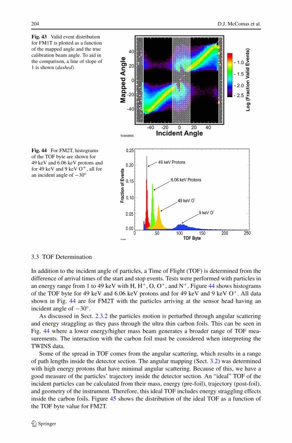
204 D.J. McComas et al.
Fig. 43 Valid event distributionfor FM1T is plotted as a functionof the mapped angle and the truecalibration beam angle. To aid inthe comparison, a line of slope of1 is shown (dashed)
Fig. 44 For FM2T, histogramsof the TOF byte are shown for49 keV and 6.06 keV protons andfor 49 keV and 9 keV O+, all foran incident angle of −30◦
3.3 TOF Determination
In addition to the incident angle of particles, a Time of Flight (TOF) is determined from thedifference of arrival times of the start and stop events. Tests were performed with particles inan energy range from 1 to 49 keV with H, H+, O, O+, and N+. Figure 44 shows histogramsof the TOF byte for 49 keV and 6.06 keV protons and for 49 keV and 9 keV O+. All datashown in Fig. 44 are for FM2T with the particles arriving at the sensor head having anincident angle of −30◦.
As discussed in Sect. 2.3.2 the particles motion is perturbed through angular scatteringand energy straggling as they pass through the ultra thin carbon foils. This can be seen inFig. 44 where a lower energy/higher mass beam generates a broader range of TOF mea-surements. The interaction with the carbon foil must be considered when interpreting theTWINS data.
Some of the spread in TOF comes from the angular scattering, which results in a rangeof path lengths inside the detector section. The angular mapping (Sect. 3.2) was determinedwith high energy protons that have minimal angular scattering. Because of this, we have agood measure of the particles’ trajectory inside the detector section. An “ideal” TOF of theincident particles can be calculated from their mass, energy (pre-foil), trajectory (post-foil),and geometry of the instrument. Therefore, this ideal TOF includes energy straggling effectsinside the carbon foils. Figure 45 shows the distribution of the ideal TOF as a function ofthe TOF byte value for FM2T.

The Two Wide-angle Imaging Neutral-atom Spectrometers (TWINS) 205
Fig. 45 The distribution of validevents over the full range ofenergies and angles are shown forFM2T as a function of ideal TOFand TOF byte value returnedfrom the TWINS instrument. Theideal TOF is calculated from theinstrument geometry, beamenergy, species, and incidentangle
For each TOF byte value, a most likely ideal TOF was defined as the peak of the distrib-ution. The most likely ideal TOF as a function of TOF byte values were fit to a second orderpolynomial to give us a mapping between TOF byte and time in seconds. The fits give thefollowing mapping from TOF byte to time for each of the four sensor heads in seconds:
TOFFM1A = −3.21 × 10⁻⁸ + 1.53 × 10⁻⁹b − 2.15 × 10⁻¹²b2 (3)
TOFFM1T = −1.63 × 10⁻⁸ + 1.39 × 10⁻⁹b − 7.87 × 10⁻¹³b2 (4)
TOFFM2A = −2.71 × 10⁻⁸ + 1.49 × 10⁻⁹b − 2.15 × 10⁻¹²b2 (5)
TOFFM2T = −2.21 × 10⁻⁸ + 1.36 × 10⁻⁹b − 1.75 × 10⁻¹²b2 (6)
where b is the TOF byte. Each sensor head has its own unique TOF conversion fit; all ofthese fits have a similar shape. Note that there are some TOF byte values that will map tonegative times of flight. These unphysical values and any TOF values that map to energiesgreater than 100 keV for hydrogen are culled out of our images.
The resolution of the TOF electronics is ∼1 ns, so the relative uncertainty is largest for thesmallest TOFs (or highest energies). However, the lowest energy particles will experiencethe largest perturbation to their motion through their interaction with the carbon foils. Theconvulsion of these two effects needs to be considered in the energy measurement. Therelative uncertainty varies as a function of incident energy and species. See Table 4 fordetails as a function of sensor head.
3.4 Mass Identification
Mass identification of ENAs is performed using the pulse height information. For two parti-cles of the same velocity, more massive particles typically result in larger start and stop pulseheights. The pulse height varies weakly with mass for the primary particles, so the stop pulseheight has less variation with mass than the start pulse height. However, the number of sec-ondary electrons liberated by passage through the thin carbon foil is also a function of themass of the particle. More massive particles liberate more secondary electrons, on average,as they pass through the thin carbon foils. This enhancement in secondary electrons alsoleads to an increase of the start pulse height for heavier ions.
A comparison for the two primary magnetospheric ions, O and H, each with the samevelocity (TOF), is shown in Fig. 46. The dependence of the pulse height on incident angleis insignificant, so to increase the statistics, we combined data from angles from −60◦ to

206 D.J. McComas et al.
Fig. 46 Comparisons of O+ andH+ start pulsed heights forparticles with the same velocity(TOF) for sensor head FM1A.Because the distributions have asignificant overlap, O+ and H+content in an image aredetermined on a statistical basis
+60◦. The pulse height distributions returned for different masses traveling at the samevelocity have different shapes and can be separated for a significant number of events on astatistical basis.
3.5 Geometric Factor
Just as the angular mapping depends on both start and stop position bytes, a similar mapis required for the geometric factor. Henderson et al. (2005) derived the geometric factorfor the MENA instrument from first principles, including effects from all elements in theparticles path, such as the fine structure of the UV rejection gratings. By using a beam thatfully illuminates the detectors over the full range of FOV, the geometric factor can be directlymeasured for each of the start—stop pixel combinations (64 Start × 256 Stop). Figure 47shows the map of the geometric factor for each of the ∼104 pixels for sensor head FM1A. Asan independent check, the measured geometric factor for TWINS generally agrees with thecalculated factor for MENA (Henderson et al. 2005) when the difference between TWINSand MENA sensors, such as the collimator and gratings geometries and number of pixels,are included.
The ‘pile up’ region at the transition between the stop and start anodes (near stop positionbytes of 110 in Fig. 47) is an artifact seen in all sensor heads. The pile up is most likely dueto secondary electrons from the foil reaching the stop anode and creating false valid events.The misalignment of the aperture and the anode is such that the aperture is closer to the stopanode on the pile up side than on the other side. The start anode is shifted toward higherbyte values, or toward the right in Fig. 12. This puts the left edge of the start anode near theedge of the aperture. Electrons from the foil will be closer to the stop anode on this side.
We performed testing with an ∼1 Sun UV source in the calibration facility. This testingshowed that as long as the line of sight to the UV source is more than 15 degrees away fromthe imaging plane of the sensor, there is no significant UV background (valid rates �1 Hz).During the seasons when the Sun direction is closest to the bore sight of the instrument(along the rotation axis of the instrument), any background from Sun exposure will onlyaffect a narrow band of scan angles, and is removed. Valid background rates were measuredto be <1 Hz during calibration. An incident flux greater than ∼100 cm−2 sr−1 s−1 keV−1
allows for reasonable imaging.

The Two Wide-angle Imaging Neutral-atom Spectrometers (TWINS) 207
Fig. 47 Map of the geometricfactor for sensor head FM1A
Fig. 48 Ion transmissionthrough the collimators for49 keV protons as a function ofincidence angle and collimatorvoltage. The top panel showsresults from a simple model,while the bottom displays resultsfrom calibration
3.6 Collimator Response
As described above, a set of biased (up to 10 kV), parallel collimators are used to rejectincident charged particles. The rejection of charged particles is a function of the particleenergy and the voltage applied to the collimator. Figure 48 shows the transmission of a49 keV H+ beam as a function of non-imaging incidence angle and collimator voltage. Thetop panel shows results of a simple model for comparison to the calibration data (bottom).At zero collimator voltage, the FOV to the ion beam is 4◦ wide, limited only by the mechan-ical obstructions of the plates. As the voltage increases, the ion beam can only transit thecollimator if it starts at larger incident angles. The electric field between the plates of the

208 D.J. McComas et al.
collimator bends the trajectories of the ions, allowing for non-normal incident particles pathto be bent into the detectors. At yet higher voltages, the transmission decreases until no ionsare passed.
The simple model of the collimator (top panel) does not include fringing fields and as-sumes that all particles that exit the collimator are detected by TWINS. Also, all particles inthe model that impact the walls are lost, while in the real instrument a small fraction scatterand create secondary events. Nonetheless, the simple model agrees well with the measureddata. Finally, the model does not include neutralization of some of the beam en route downthe beam line, although this component is clearly evident in the data. The signal at incidenceangle of 0◦ for all collimator voltages in the bottom panel is the neutral component of thecalibration beam, which is created by charge-exchange with the residual background gas inthe calibration facility flight tube. At the SwRI Instrument Calibration Facility, the fractionof the ion beam that is converted into a neutral beam is typically 1 to 5%.
The collimators effectively exclude particles with energy per charge <12 times the col-limator voltage. When the collimators are operating at their full voltage of 10 kV, only thevery low fluxes of ions with energies >120 keV will be able to pass the collimator.
At the start of the mission, the collimator voltages were set to a value of 6500 volts on allsensor heads. This value was chosen to give us good ion rejection while allowing the optionof increasing this voltage in the future.
3.7 Calibration Summary
Table 4 lists the detailed response for each sensor head. The upper bound of the energyrange is defined as the lowest energy bin >100 keV for an incident angle of 30◦. The TOFis capable of measuring higher energies (shorter times of flight), but the collimator is unableto reject particles above this energy. Measurements of the relative energy and angular reso-lution are the FWHM of the distribution of measured valid events compared to the knownincident calibration source.
4 TWINS Data and Science Analysis
Data from TWINS is made available to the scientific community and to the general publicas quickly as possible after acquisition. The TWINS Science Operations Center (SOC) val-idates the data and produces higher-level products useful for scientific and educational pur-poses. TWINS Education and Public Outreach (EPO) includes providing data to the publicand communicating the excitement of the first 3-D visualization of the structure and dynam-ics of the Earth’s magnetosphere.
4.1 TWINS Science Data
TWINS has four science modes of operation: Static Test, Static Imaging, Dynamic Test, andDynamic Imaging (Table 5). In each of these modes housekeeping data, Starts, Stops, andValid Event Rates, as well as direct events are returned as part of the data stream. For thetwo “imaging” modes, the telemetry includes images which are produced onboard the space-craft. For the two “test” modes, no onboard images are produced, allowing more telemetryfor direct events data. The static modes maintain a time-synchronized telemetry output suchthat one sample is provided each 1.333 s. The Dynamic modes are used when rotating the

The Two Wide-angle Imaging Neutral-atom Spectrometers (TWINS) 209
Table 5 Data mode types and properties
Mode Onboard images? Sector size # sectors per scan at3◦/sector rotation(60 s image)
# of direct eventstransmitted per sector
Static test No 1.333 s 45 1566
Static imaging Yes 1.333 s 45 956
Dynamic test No 4◦ 45 1863
Dynamic imaging Yes 4◦ 45 1253
instrument. Dynamic Imaging mode is position-synchronized such that one sample is pro-duced for each 4◦ sector of rotation, which at the nominal rotation rate of 3◦ s−1, takes1.333 s. The normal science operating mode is Dynamic Imaging.
TWINS’ main telemetry product is “direct events” data, in which we transmit a numberof pieces of information about individual particles measured by the detector. The numberof direct events per sector depends on the data mode: 1253 for dynamic imaging, 1863 fordynamic test, 956 for static imaging, and 1566 for static test. The direct events parametersare:
1) Time of flight (8 bits, so 256 possible values)2) Start height (8 bits, so 256 possible values)3) Start position (6 bits, so 64 possible values)4) Stop height (7 bits, so 128 possible values)5) Stop position (8 bits, so 256 possible values)6) “slice” (2 bits, so 4 possible values), which gives azimuth with 0.333 sec resolution
(∼1◦).7) head (1 bit, so 2 possible values), toward or away sensor head.
While in the Imaging modes, TWINS uses a portion of the telemetry stream that wouldotherwise be used for Direct Event data to send down an onboard image. The direct eventdata is processed to create an image of ENA incident angle, speed, and species. Geometricfactor determination is less precise for the onboard processing, so direct event images shouldbe used for most scientific analysis. The onboard images are included to cover times whenthe rate of direct events exceeds the available telemetry of 37.6 kb/s allocated for directevents. This translates to a maximum rate of 1253 direct events counts per 4◦ telemetrysector during normal Dynamic Imaging Mode. During these high rate times the number ofdirect events that can be telemetered down may only be a fraction of the total valid events.Furthermore, because the direct events are sent down on a first-come-first-served basis, therecan be gaps in coverage when the number of direct events exceeds the telemetry allocation.
Figure 49 shows the angle derived from the onboard image processing over the full rangeof incident beam directions. The angle derived onboard is plotted as a function of the inci-dent angle of the calibration beam. The dashed white line of slope 1 is added for a visualguide. We use a conservative culling scheme on board in order to ensure that ENAs includedin the onboard images are real. All culled events are summed together at 0◦ in this image (alocation within the blind spot and thus unphysical) so that we know how many events havebeen culled.

210 D.J. McComas et al.
Fig. 49 Angle determined by theonboard image processing as afunction of the incident angle ofthe 31 keV proton beam in acalibration run from FM2T
4.2 The TWINS Science Operations Center and Science Data System (SDS)
For most scientific applications, pre-generated TWINS images and ancillary data plotsshould be adequate. These products are available through a public-access page (http://twins.swri.edu) with a web-based selection tool. Users of this public page can browse sequentiallythrough TWINS images as well as other support plots and data.
TWINS Team members and other scientists who need more detailed and flexible accessto TWINS data can use the capabilities of the Science Data System (SDS), developed specif-ically for TWINS. The SDS is composed of a database server (DBS) and web user-interface(WUI). All mission data will reside in the DBS, which currently consists of 3 terabytes ofRAID storage (2.5 TB after partitioning) and uses an Oracle data base system. The data isaccessed via an interface employing Structured Query Language (SQL), run on a dedicatedUNIX/LINUX server. TWINS mission data includes ENA and LAD science data, house-keeping data, laboratory calibration data, and ancillary (e.g., geomagnetic and solar wind)data. Science and housekeeping data are entered into the DBS upon arrival (in the formof DVDs) at SwRI, and automatically processed to create products such as browse sciencedata. Initial data processing maps instrument counts onto geomagnetic and geographic co-ordinate systems so that images may be easily compared to each other and to previous andcomplementary data sets. These images are then validated by the SOC. All calibration datawere previously fed to the DBS after acquisition in the calibration facilities at SwRI andreside there for further analysis as needed in support of space-based observations. Ancillarydata is entered into the DBS by automatic updating scripts.
After processing and validation, all data are archived at SwRI. The time frame for datavalidation ranges from hours to months depending on the complexity of the validation forthe specific data product. One basic data type for TWINS is an “image;” i.e., a 1-minutehistogram of instrument counts as a function of azimuth, polar angle, velocity and mass.Raw, validated data and histograms corrected for instrument response are archived. Lyman-α data, consisting of counts as a function of look direction, are also archived. In addition, wearchive higher-level data products, including both single spacecraft and stereo images. Wealso provide TWINS data to the National Space Science Data Center (NSSDC) to facilitateadditional dissemination to the broader scientific community and additional archiving atNASA. Archive copies of raw data DVDs are kept at LANL and NSSDC. All TWINS SDSsoftware is backed up at SwRI and LANL.

The Two Wide-angle Imaging Neutral-atom Spectrometers (TWINS) 211
4.3 Achieving Closure on TWINS Science Objectives
The TWINS team has identified specific and detailed research objectives, which canuniquely be addressed by simultaneous dual-point ENA observations. The interpretationand science extraction activities with stereo imaging are multifaceted. A first level of inter-pretation simply uses the 3-D visualization of the structures and evolution of the imagedregions; these direct observations enable the examination of temporal and spatial correla-tions between the different regions. The next step is to incorporate ancillary data sets inthese analyses, including observations such as solar wind, geosynchronous and low alti-tude spacecraft observations and measurements, and geomagnetic indices and other groundobservations. As described above, the TWINS SOC has been designed to easily and effi-ciently incorporate such correlative observations. Quantitative parameter extraction of thedetailed plasma distributions will be carried out using various levels of image unfolding or“inversion” techniques (see below). Such quantitative information allows us to attack theproblems of global electrodynamics for some regions. Finally, careful comparisons will bemade between the evolving images and predictions based on first principle simulations.
TWINS also provides global images as context for other detailed magnetospheric andsolar-terrestrial studies. We share these new images of the Earth’s plasma environs with theresearch community and the public. Rapid and frequent access to the TWINS stereo imagesis facilitated with software and displays that allow the creation of easily-understood imagesand movies from the TWINS data set. We expect that the TWINS data will enable newapproaches for researchers working on other magnetospheric and ionospheric problems.Thus, in addition to the on-line images, we also provide more quantitative and detailedanalysis results as rapidly as possible so that space scientists can readily ascertain the stateof the solar wind-magnetosphere-ionosphere system.
4.4 Inversion of TWINS ENA Images to Extract Global Energetic Ion Distributions
The TWINS sensors collect ENA images of the global distribution of energetic ions fromtwo independent vantage points. Image inversion is needed to determine the behavior ofthe ion populations from the ENA images. Inversion procedures have been in operation forseveral years on the single vantage point data from the IMAGE HENA and MENA cameras(De Majistre et al. 2004; Perez et al. 2004a, 2004b). The basic technique for inversion ofindividual images is summarized in Appendix B. We describe here generalization of thistechnique to two (stereoscopic) images and quantitative measures are given of how much thestereo viewpoints from TWINS will improve the spatial resolution of the extracted energeticion distributions.
4.4.1 Generalization to Inversions Using TWINS Stereo ENA Images
The general nature of the inversion technique described in Appendix B does not formallylimit the input ENA data to measurements from a single vantage point or instrument. Allthe information about the vantage point and instrument response is contained in the kernel,K, so measurements from any point with any instrument can be included in the inversion aslong as the geometry and response are known. That is, (B.11) can be made to accommodatemultiple vantage points by putting
∣∣∣∣∣∣∣∣∣
C1
C2...
Cm
∣∣∣∣∣∣∣∣∣=
∣∣∣∣∣∣∣∣∣
K1
K2...
Km
∣∣∣∣∣∣∣∣∣Jion (7)

212 D.J. McComas et al.
where the subscripts label the measurements and kernels appropriate for single vantage pointmeasurements.
It is important to note at this point that the TWINS images used in the multiple vantagepoint retrieval are acquired from essentially four different cameras, i.e., platforms on twospacecraft with two imaging heads each. Since information is being combined from thesefour data sources into a single ion distribution, the heads must be closely cross-calibrated toavoid systematic errors in the retrievals.
Various products of the kernel and the generalized inverse can be used to study the effec-tiveness of the inversions (Menke 1989). The most obvious measure of retrieval quality isthe covariance of the retrieval, which by standard error propagation is
σ 2j = Gσ 2
CGT . (8)
The diagonal of this matrix is the expected variance in the retrieved quantities. We expectthe variance for the multipoint retrievals to be smaller than the retrievals from single van-tage points. The amount of reduction for various observation scenarios provides us with ameasure of the quality of the retrieval.
Another important metric is the spatial resolution of the retrieval. This can be studiedwith the so-called model resolution matrix (Menke 1989), A, defined as
A = GK. (9)
For an exact retrieval, A should be the identity matrix, as can be seen by pre-multiplying(B.11) by the generalized inverse and using (B.13)
GC = GKJion
J̃ion = AJion
(10)
where we have put J̃ion for the retrieved ion distribution to distinguish it from the true iondistribution, Jion. In most cases A has off diagonal elements—this represents a degradationof the resolution of the inversion. That is, if the ion distribution were zero everywhere withthe exception of a single element of Jion, after measurement and inversion, the resultingestimated ion distribution would spread away from that single element. For this reason, thedegree to which the elements on the diagonal of A differ from unity is a good measure ofthe spatial resolution of the inversion.
4.4.2 Simulations of Inversions of Stereo TWINS Images
We present here a simulation of a TWINS-like multi-vantage point retrieval. For this simu-lation, we place two ENA imagers at 8 earth radii in the dawn/dusk plane, each 30◦ abovethe magnetic equator, one on the dawn side, one on the dusk side. For convenience we haveused the existing IMAGE/HENA camera response function. There should not be any sub-stantial differences in the characteristics of the inversions or the measures of their accuracy,because the basic principles of stereo image inversion are the same for both the cameras onIMAGE/HENA and TWINS. To demonstrate the improvement resulting from dual vantagepoint observations, we also present results from a single vantage point measurement wherethe instrument is located at 8 earth radii above the magnetic pole. The equatorial ion inten-sities used in the simulation are depicted in the center panels of Fig. 50 for the intensitiesperpendicular (μ = 0) and parallel (μ = ±1) to the equatorial field lines (given on the left

The Two Wide-angle Imaging Neutral-atom Spectrometers (TWINS) 213
Fig. 50 Simulated retrieval results from an anisotropic ion pitch angle distribution. The right and left showthe parallel and perpendicular moments of the pitch angle distribution for each case. Center: ion intensitydistribution input to the simulation. Top: retrieved distribution for a single observer over the North magneticpole. Lower: retrieved distribution for dual vantage taken in the dawn/dusk plane 30◦ above the magneticequator (TWINS-like observations). The common (logarithmic) color bar gives the differential intensitiesplotted in all six panels

214 D.J. McComas et al.
Fig. 51 Estimated variance for (a) the single vantage point retrievals, and (b) dual vantage point retrievals
and right sides, respectively). These ion intensities are used to generate simulated imagesat the given vantage points. We then invert the simulated images, and for a perfect retrievalthe result should be identical to the input ion intensities. The top panel of Fig. 50 shows theresults of this simulate and retrieve process for an observer looking down from the Northmagnetic pole. The bottom panel shows the results for a dual vantage point (TWINS-like)observation.
The simulated ENA images include randomly generated Poisson counting statistics ineach pixel. In this figure areas with negative values are set to white. This occurs predomi-nantly on the dayside because of very low counting rates on the day side. We see that thedual vantage point retrieval shows better agreement at the peak, whereas the single vantagepoint retrieval tends to broaden the peak somewhat. We also see that away from the peak,the effect of the Poisson noise is more significant for the single point retrieval.
4.4.3 Quantitative Measures of the Improvements in Inversion Using Stereo TWINS Images
In order to quantify this comparison, we show the results of the covariance and spread analy-sis. In Fig. 51 we present the estimated variance for the two retrievals shown in Fig. 50. Wesee that for the dual point retrieval that the variance is much smaller, particularly in the dawndusk sectors. Further, the performance of the dual retrieval is much improved at higher L
values.In Fig. 52 we give the results of the spread analysis. For this figure, we plot the difference
of the diagonal of the resolution matrix, A, from unity. For a perfect retrieval, this quantitywould be zero everywhere. The dual vantage point retrieval is clearly superior according tothis metric, particularly for L > 4. This is born out in the retrieval results shown in Fig. 51that show visible spreading of the peak in the single vantage point retrieval that is not nearlyas apparent in the dual point result. These results quantitatively demonstrate the significantimprovement over single-point images that will be made by the stereo images from TWINS.
5 Initial Stereo Observations from TWINS-1 and -2
The TWINS-1 and TWINS-2 instruments were launched on two separate non-NASA U.S.government spacecraft (respectively) in 2006 and 2008, respectively. After checkout and
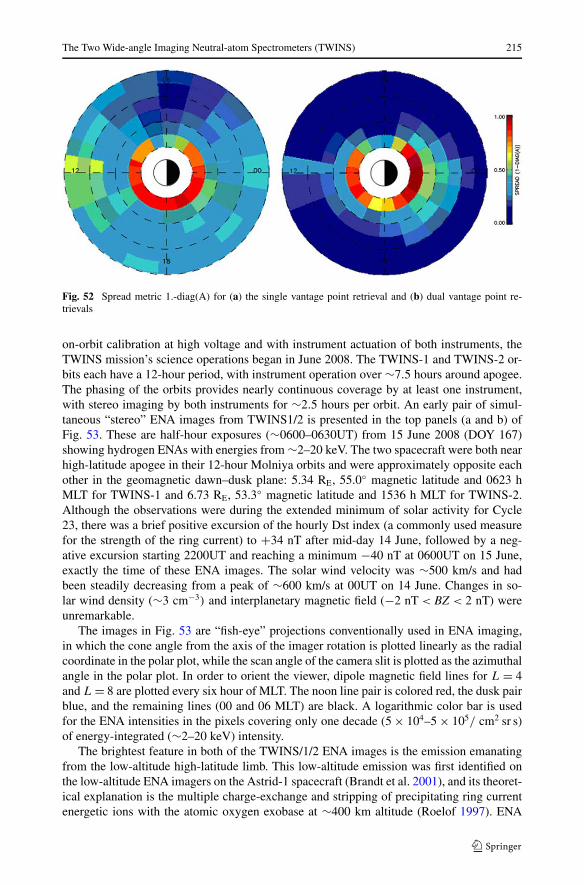
The Two Wide-angle Imaging Neutral-atom Spectrometers (TWINS) 215
Fig. 52 Spread metric 1.-diag(A) for (a) the single vantage point retrieval and (b) dual vantage point re-trievals
on-orbit calibration at high voltage and with instrument actuation of both instruments, theTWINS mission’s science operations began in June 2008. The TWINS-1 and TWINS-2 or-bits each have a 12-hour period, with instrument operation over ∼7.5 hours around apogee.The phasing of the orbits provides nearly continuous coverage by at least one instrument,with stereo imaging by both instruments for ∼2.5 hours per orbit. An early pair of simul-taneous “stereo” ENA images from TWINS1/2 is presented in the top panels (a and b) ofFig. 53. These are half-hour exposures (∼0600–0630UT) from 15 June 2008 (DOY 167)showing hydrogen ENAs with energies from ∼2–20 keV. The two spacecraft were both nearhigh-latitude apogee in their 12-hour Molniya orbits and were approximately opposite eachother in the geomagnetic dawn–dusk plane: 5.34 RE, 55.0◦ magnetic latitude and 0623 hMLT for TWINS-1 and 6.73 RE, 53.3◦ magnetic latitude and 1536 h MLT for TWINS-2.Although the observations were during the extended minimum of solar activity for Cycle23, there was a brief positive excursion of the hourly Dst index (a commonly used measurefor the strength of the ring current) to +34 nT after mid-day 14 June, followed by a neg-ative excursion starting 2200UT and reaching a minimum −40 nT at 0600UT on 15 June,exactly the time of these ENA images. The solar wind velocity was ∼500 km/s and hadbeen steadily decreasing from a peak of ∼600 km/s at 00UT on 14 June. Changes in so-lar wind density (∼3 cm−3) and interplanetary magnetic field (−2 nT < BZ < 2 nT) wereunremarkable.
The images in Fig. 53 are “fish-eye” projections conventionally used in ENA imaging,in which the cone angle from the axis of the imager rotation is plotted linearly as the radialcoordinate in the polar plot, while the scan angle of the camera slit is plotted as the azimuthalangle in the polar plot. In order to orient the viewer, dipole magnetic field lines for L = 4and L = 8 are plotted every six hour of MLT. The noon line pair is colored red, the dusk pairblue, and the remaining lines (00 and 06 MLT) are black. A logarithmic color bar is usedfor the ENA intensities in the pixels covering only one decade (5 × 10⁴–5 × 10⁵/ cm2 sr s)of energy-integrated (∼2–20 keV) intensity.
The brightest feature in both of the TWINS/1/2 ENA images is the emission emanatingfrom the low-altitude high-latitude limb. This low-altitude emission was first identified onthe low-altitude ENA imagers on the Astrid-1 spacecraft (Brandt et al. 2001), and its theoret-ical explanation is the multiple charge-exchange and stripping of precipitating ring currentenergetic ions with the atomic oxygen exobase at ∼400 km altitude (Roelof 1997). ENA

216 D.J. McComas et al.
Fig. 53 Simultaneous fish-eye “stereo” ENA images ∼0600–0630 UT 15 June 2008 (DOY 167) from (a)TWINS1 near dawn (5.34 RE, 55.0◦ magnetic latitude and 0623 h MLT) and (b) TWINS2 near dusk (6.73 RE,53.3◦ magnetic latitude and 1536 h MLT). Dipole magnetic field lines are drawn at L = 4 and L = 8, withthose at 1200 h MLT (noon) in red and those at 1800 h MLT in blue, while midnight and dawn are inblack. The Earth’s limb and terminator are delimited. The intensities in each pixel are summed over theenergy range ∼2–20 keV, assuming ENA hydrogen. The logarithmic color bar spans one decade of intensity(5 × 10⁴–5 × 105 cm−2 sr−1 s−1). The highest intensities stem from low-altitude emission from the Earth’satomic oxygen exobase ∼400 km (see text). Even for this relatively weak geomagnetic activity, higher altitudeemission is also clearly visible above instrument background emanating from the nightside ring current regionL ∼ 4. Corresponding simulations of the ENA images are shown in panels (c) and (d) and described inFig. 54(a)
cameras on the later IMAGE spacecraft (MENA and HENA) revealed that the low-altitudeemission was a common occurrence whose intensity depended on both the MLT distributionof the precipitating ion intensity and the viewing perspective from the spacecraft. The low-altitude emission tends to appear when the spacecraft is at high latitudes and above the limbopposite to the spacecraft MLT.

The Two Wide-angle Imaging Neutral-atom Spectrometers (TWINS) 217
Fig. 54 (a) Distribution of energetic proton intensity in the magnetic equatorial plane (arbitrary units) usedto produce the simulations in Figs. 53(c) and 53(d) of the observed TWINS ENA images in Figs. 53(a)and 53(b) from the spacecraft positions near dawn and dusk, respectively. The THEMIS-D orbit during 15June 2008 is projected into the equatorial plane. Note that it enters the ring current region L < 8 (movingcounter-clockwise) at ∼0600 UT (the time of the half-hour exposures of the TWINS images). (b) Com-parison of the ion pressure (<30 keV) measured on THEMIS-D (black curves, nPa) with the normalizedintensity (green curves, arbitrary units) of the model energetic proton intensity (Fig. 54(a)) used to simulatethe TWINS1/2 ENA intensities in Figs. 53(c) and 53(d)). THEMIS-D ion pressure courtesy of A.T.Y. Lui[private communication]
At higher altitudes in these TWINS images, ENA emission may be seen above the instru-ment background in the nightside inner ring current region (L < 4). However, the line-of-sight projection effects are significant, so the parent ion distribution must be unfolded fromthe ENA images. We do this by forward modeling the ENA emission. The hydrogen geo-corona model is taken from Østgaard et al. (2003). We specify the magnetic equatorial iondistribution using a 32-parameter model (Roelof and Skinner 2000). For these initial images,we simplify the model by assuming an isotropic pitch-angle distribution. The remaining pa-rameters describing the distribution in dipole L and MLT are adjusted until the simulatedENA images match (by eye, in this first effort) both of the TWINS1/2 images. The model dis-tribution is depicted in Fig. 54(a), and the simulated ENA images are presented in the lowerpanels (c) and (d) of Fig. 53. The simulation includes an approximation (Gaussian) to theinstrument point-spread function, but omits any instrumental backgrounds. The low-altitudeemission is approximated by adjusting the exospheric oxygen density and scale height andassuming only a single charge-exchange and stripping interaction for nearly-mirroring pre-cipitating energetic ions, with no emission coming from below this “hard shell” at 500 kmaltitude. These approximations constitute an extreme over-simplification of the actual multi-collisional ENA albedo, but they are adequate for these images because we make no attemptto extract the actual low-altitude intensities. Given all these approximations, we considerthat the simulated low and high altitude ENA emission patterns (Figs. 53(c) and 53(d)) arein good agreement with the patterns in the TWINS1/2 images (Figs. 53(a) and 53(b), re-spectively).
Further confirmation of the forward simulation of the high-altitude emission comes froma comparison with the in situ measurement of the <30 keV ion pressure measurements fromthe electrostatic analyzer on board the THEMIS-D spacecraft (A.T.Y. Lui, private commu-nication). THEMIS-D was just beginning a pass through the ring current region (L < 8) at

218 D.J. McComas et al.
∼0600 UT on 15 June (the beginning time of the TWINS1/2 stereo half-hour image expo-sures in Figs. 53(a) and 53(b)). Its trajectory is over-plotted on the forward-model equato-rial ion intensity distribution in Fig. 54(a). Figure 54(b) compares the time history of theTHEMIS-D <30 keV ion pressure during its day-long pass through the ring current withthe corresponding trace (Fig. 54(a)) through the normalized (arbitrary units) ion intensityused in the forward-modeled TWINS1/2 images of Figs. 53(c) and 53(d). Although thesetwo quantities (in situ measured pressure <30 keV and image-forward-modeled ion inten-sity) are not strictly equivalent, the agreement of their general trends tends to validate theforward modeling. Even though the modeled ion intensity does not show the peak near theinner edge of the ring current, the actual edges themselves agree closely. This is quite mean-ingful, because the inner edge was adjusted to fit the ENA images, not the THEMIS pressureprofiles.
These initial stereo images from the TWINS spacecraft during a time of relatively mod-est geomagnetic activity show the quality and utility of such stereo observations and pointtoward the future harvest of magnetospheric science from this first ENA “stereo” mission.With more sophisticated analysis of such simultaneous ENA images, we expect to unfoldmany new signatures of phenomenology revealed by ENA emission at both high and lowaltitudes.
6 Conclusions
TWINS is a remarkable mission that allows the visualization of the 3-D structure of themagnetosphere from global stereo imaging for the first time. This is accomplished using en-ergetic neutral atom images, produced over a broad energy range of magnetospheric plasmaenergies, with simultaneous observations from two widely spaced observing platforms.
This paper has documented the TWINS instruments, their design, construction, calibra-tions, and instrument modeling. In addition to detailed stereo ENA measurements, TWINSmakes Lyman-α observations of the geocorona that produces the ENAs and is supportedby environmental monitors on the same spacecraft. This paper has also discussed some ofthe analysis plans, at least one inversion technique that will be used to assemble the stereoimages into a combined model of the 3-D plasma distributions, and shown some “first light”stereo images simultaneously from the TWINS-1 and -2 spacecraft. Finally, in the Appen-dix, we document the Southwest Research Institute Calibration Facility, which was used forall TWINS flight calibrations.
Acknowledgements The TWINS Mission-of-Opportunity is dedicated to the memory of Phil Barker, whowas the original TWINS Project Manager and served in that capacity until his death in 2003. Phil was a goodfriend to the entire TWINS team, and his brave battle with colon cancer throughout the development of muchof the TWINS mission hardware was an inspiration to the team. Figure 8 shows the plaque that was placedon the TWINS instrument (under the LAD) to commemorate his dedication to this project. We thank EricArchuleta, Donna Avila, Steve Battel, Randy Bremmer, Kent Bress, Dana Burket, Jim Byrd, Butch Carruth,Rick Claffy, Jim Cravens, Bill Davis, Dot Delapp, Greg Dirks, Eric Dors, Karen Douglas, Reginald Eason,Gus Escobar, Brian Gupta, Mike Henderson, Brad Johnson, Roger Kraus, Mike Lampton, Glen Martin, DaveMengers, Thomas E. Moore, A. M. Niazy, Enold Pierre-Louis, Jillian Redfern, Mark Schattenburg, MikeVan Dyke, Mike Wallace, and the numerous other dedicated men and women who contributed to the successof the TWINS program. In addition, we are particularly indebted to Wendy Mills for all of her help in as-sembling and editing this paper and to Colonel John D. Cunningham, USAF (Ret.) for his crucial support ofthe TWINS project. TWINS was funded by the National Aeronautics and Space Administration through theGSFC Explorer’s Office.

The Two Wide-angle Imaging Neutral-atom Spectrometers (TWINS) 219
Fig. 55 The Southwest ResearchInstitute (SwRI) InstrumentCalibration Facility is shown inthis photograph. The mainvacuum vessel has anapproximate volume of 1400liters. Access to the interior ofthe chamber is through a Vitonsealed door inside a class 10,000clean tent. A class 100 cleanbench is also inside the clean tentto allow for any final work to beperformed on the instrumentprior to installation into thevacuum chamber. A ring ofvacuum feedthroughs of varyingsizes circle the chamber in aplane with the beam line. Thefeedthroughs are accessedoutside the clean tent
Appendix A: The Southwest Research Institute Instrument Calibration Facility
A.1 Introduction
The Southwest Research Institute (SwRI) Instrument Calibration Facility (Fig. 55) is usedto prototype, develop, and calibrate space flight plasma instruments and ENA imagers. Thisfacility has been in operation in its present location for over 15 years and has been used asthe calibration facility for magnetospheric (IMAGE/MENA (Pollock et al. 2000)), planetarymagnetospheres (Cassini/CAPS (Young et al. 2004)), solar wind dynamics (SWAP (McCo-mas et al. 2007)), and cometary (Rosetta/IES (Burch et al. 2007)) missions in addition totesting numerous instrument prototypes.
Starting in the fall of 2000 we undertook an extensive upgrade of the facility, reworkingvirtually every aspect of it other than the ion source itself. This upgrade rectified a number oflimitations in the earlier configuration and leveraged the best practices and lessons learnedfrom a number of world class facilities including, principally, the ion calibration facilityat Los Alamos National Laboratory. This appendix describes the current state of SwRI’sfacility, which continues to evolve as new projects require enhanced or new capabilities.Differences from the configuration at the time of the TWINS calibration are noted.
In Sect. A.2 we describe the vacuum system and general lab layout. Section A.3 describesthe ion source and ion optics. The positioning system is described in Sect. A.4.
A.2 Vacuum System and Lab Layout
Space plasma and ENA instruments typically use either MCPs and/or CEMs to detect sin-gle electrons, ions, or neutral atoms. Both of these types of detectors are extremely conta-mination sensitive, especially to complex hydrocarbons (e.g., McComas and Bame 1984;McComas et al. 1987, and references therein). Because it is not possible to replace detectorsafter launch, every effort must be made to maximize their useful lifetimes; this requirementdrives absolute cleanliness and the best possible vacuum conditions reasonably achievable.
The control of the vacuum system was designed with instrument safety as the primaryconcern. All valves and pumps are controlled through a central control panel. This panel has

220 D.J. McComas et al.
Fig. 56 This schematic shows the layout of the vacuum components of the calibration facility. Only dryvacuum pumps are used in this system to minimize the possibility of contamination to the instruments undertest. Cleanliness of the vacuum is monitored with a 200 AMU Residual Gas Analyzer (RGA)
internal logic that limits the actions available to the operator to prevent ‘unsafe’ actions. Forexample, venting of the system is not allowed while the chamber is being actively pumped.In the event of loss of power to the facility, all valves automatically close and the pumpsturned off. The control system requires user intervention to bring the system back online.This is to prevent a valve from opening into an unsafe state when power is re-established.The central control panel will also take action to isolate identified unsafe conditions or faultsbased on pressure and temperature monitors. If an overpressure is detected in one region ofthe vacuum system, valves close to isolate that portion of the system.
The vacuum chamber is divided into subsections, each pumped independently and shownschematically in Fig. 56. Each subsection can be valved off from the other subsections andbe brought up to atmosphere while the others are held at HV. These subsections are allserviced by a common oil-free rough vacuum line that can pump them down independentlyfrom atmosphere to a low cross over pressure.
The first subsection is the main vacuum vessel. This vessel is a domed cylinder witha 122 cm (48 in) diameter and 213 cm (84 in) length. Test objects are mounted on a 4-axis positioning system (Sect. A.4). HV pumping is supplied by 2 Helix-CTI Cryo-Torr 10Cryogenic pumps, each with a 3000 l/s pumping speed. These pumps were chosen for thepumping speed and cleanliness. If one pump suffers a failure and has to be isolated, thepumping capacity of the other pump is sufficient to maintain the main vessel at HV levels,providing a level of redundancy in the vacuum system. The vacuum pressure is monitoredby two independent Pfeiffer PBR 260 Pirani/Hot Filament full range pressure gauges. Thecleanliness of the vacuum is monitored with a Dycor Dymaxion Residual Gas Analyzer(RGA) that measures up to a mass of 200 AMU. The ultimate pressure of the main vessel is<1 × 10⁻⁸ Torr with the RGA typically showing essentially no higher mass contaminants(>50 amu) above ∼10−13 Torr.

The Two Wide-angle Imaging Neutral-atom Spectrometers (TWINS) 221
The next subsystem is the “Science” chamber. The science chamber and the main vacuumvessel are connected by a 13.25′′ gate valve. This vessel is a domed cylinder with a 45 cmdiameter and 77 cm length. HV pumping is supplied by a Varian Cryogenic pump with a1500 l/s pumping speed. High vacuum is monitored by a Pfeiffer PBR 260 Pirani / Hot Fil-ament full range pressure gauge. The cleanliness of the vacuum is monitored with anotherDycor Dymaxion RGA. When the 13.25′′ gate valve between the science chamber and themain vacuum vessel is open, the cryogenic pump in the science chamber assists in the pump-ing of the main vacuum vessel. This adds to the pumping speed and capacity of the mainvacuum chamber. The ultimate pressure of the science chamber is similarly <1 × 10⁻⁸ Torrwith essentially no higher mass contaminants (>50 amu) above ∼10−13 Torr.
All access to the main vessel and the science chamber is through a Class 10,000 cleantent, visible in Fig. 55. Both chamber doors open into this clean tent. This tent has a Class100 clean bench with ESD monitors. The ESD monitors are tied to the vacuum chamberwalls and to Earth ground through grounding wells. High purity N2 is available in the cleantent for instrument purge. A series of 2.75, 8, 10, and 13.25 inch Con-Flat flanges are avail-able for electrical and mechanical feed throughs. These feed throughs are outside the cleantent to allow for instrument GSE to be set up without compromising the clean area. Allflanges are the Con-Flat type except for the chamber doors. The main chamber door andscience chamber both use a Viton seal.
The final subsystem is the ion optics/flight tube. The science chamber and the flighttube are connected by another 13.25′′ gate valve and the ion optics has a line of sight tothe main chamber through the science chamber. The main flight tube cylinder is 25 cm indiameter and 2.5 m long. The cylinder that comprises the optics section is 15 cm in diameterand 1 m long and is pumped by a Shimadzu magnetically levitated turbo mechanical dragpump (labeled Mag. Lev. in Fig. 56), with a pumping speed of 400 l/s. A turbo pump isrequired for this section to pump out the source gas used in the ion source (Sect. A.3). Highvacuum is monitored by a pair of two independent Pfeiffer PBR 260 Pirani/Hot Filamentfull range pressure gauges. The ultimate pressure in this subsection is <1×10⁻⁷ Torr. Sincethe TWINS calibration, a gate valve has been added between the flight tube and ion opticssection. The flight tube is pumped by a 1000 l/s Shimadzu pump. Both magnetically levitatedpumps are backed by the same BOC Edwards scroll pump.
All vacuum subsections are serviced by a common rough vacuum line. The rough vac-uum line is pumped with a combination of a BOC Edwards scroll pump and a Drytel 100series pump. This rough line also is used for in the regeneration of the cryogenic pumps.Venting of all sections and pumps is performed with High purity (99.999%) N2. The timeto crossing over to the HV pumps is 45 minutes for the main chamber, 8 minutes for thescience chamber, and 5 minutes for the flight tube/ion source.
A.3 Ion Source and Optics
SwRI’s calibration facility can produce a high quality, stable beam of positive ions, nega-tive ions and neutral atoms at any energy between 500 eV–50 keV with masses from 1 to>40 AMU (higher mass beams can be produced at reduced energies). The facility uses aPeabody Scientific Model PS-100 DuoPlasmatron as its primary ion source. Ions are ex-tracted from this source with a typical energy per charge of 500 eV/q–1.5 keV/q, howeverthis value is adjustable. Stability of the output of a DuoPlasmatron ion source is directlylinked to the stability of the gas pressure in the ion source. To maintain a constant pressurein the ion source during TWINS’ calibration, a Granville-Phillips model 216 pressure con-troller was used to control the flow of the source gas. (recently changed to a MKS 250E

222 D.J. McComas et al.
Fig. 57 The ion beam optics is shown in this schematic view. The ion source generates a range of ionspecies and charge states. These ions are extracted from the source with an energy of approximately 1000 eVper charge. The Einzel lens focuses the extracted beam into a Wien filter. The Wien filter is used to select themass per charge of the species to be passed through the raster plates. The raster plates are used to steer theion beam and to expand the beam size. The whole optics section can then be floated up to 50 kV to set thefinal energy of the calibration ion beam. The polarity of the optics can be reversed to work with negative ions
pressure controller). Variation of the beam is maintained to <5% for long (hours) periods oftime.
The ion beam is focused and tuned through an electro optic system (Fig. 57). The ionsthat are extracted from the source first pass through an Einzel lens to focus the beam. Afterthe Einzel lens, the beam passes through a Wien (E × B) filter, which selects the massper charge to be transmitted. This filter has a resolution of M/�M of >50. A 3◦ bendimmediately following the Wien filter deflects the beam, effectively removing other massions, neutral particles and photons exiting the ion source.
Following the 3◦ bend, a set of raster plates are used to steer the beam and to expand thebeam to allow for illuminating a large area. The raster system controls allow for adjustmentof the DC offset and for the amplitude of the raster. The raster has a frequency of 6.85 kHz inthe horizontal direction and 1.22 kHz in the vertical. The nominal beam diameter in the mainvacuum vessel is 1.5 cm, but can be rastered up to 10 s of cm. In the normal configuration,the size of the beam is limited by a 10 cm diameter circular aperture at the entrance of themain vacuum vessel. See Dempsey (1997) for electro optical ray tracing of this facility.
The electro-optics system can be biased to allow for the extraction of either a positiveor negative ion beams. The ion source and all ion optics are floated between −50 kV and+50 kV, depending on the ultimate energy desired. The total energy per charge is then thesum of the ∼1 kV/q extraction potential and the float potential. All control electronics for theoptics and ion source are floated at the same potential as the ion optics (up to 50 kV). Com-munication between the control electronics and the floating source is performed throughfiber optic cables to prevent high voltage breakdown. The ion source requires active coolingusing Galden HT200 high dielectric fluid. The spread in the beam energy comes from thethermal spread in the ion source and is independent of the final energy. The energy spreadin the source is low (∼1.5 eV) including the energy spread in the ion source region andsubsequent E × B filter.

The Two Wide-angle Imaging Neutral-atom Spectrometers (TWINS) 223
After being accelerated to its final energy, selected in the E × B filter, and rastered tothe appropriate size, the ion beam passes through an ∼2.5 m long field free flight tube. Thistube has knife-edged collimating discs spaced throughout its length to limit any forwardscattering of particles. The length of the flight tube limits passage to only particles withtrajectories nearly parallel to the beam line. The final beam at the main vacuum vessel has ameasured angular spread of <1◦.
The beam flux is monitored by a combination of detectors. The low flux beams typicallyrequired for calibration are monitored with an Amptektron Model 501 particle detector. Inaddition to the Amptektron, a Faraday cup is also be used at higher flux levels. Both theAmptektron and the Faraday cup are mounted on a linear actuator just ahead of the sciencechamber so either of these detectors may be deployed into the beam and retracted when notin use.
Our typical operation is to measure the beam flux periodically throughout the calibrationof an instrument as a measure of the constancy of the beam. In addition, these detectorsare used to give the beam operator feedback when adjustments are made in energy, flux,or other beam parameters. The uniformity of the ion beam is monitored by a large area(100 × 80 mm) MCP imaging detector, Quantar model 3398A. To prevent saturation of theimaging electronics, the large imager is mounted behind a low transmission grid (10%). Thisdetector is mounted on its own dedicated motion stage at the entrance to the main vacuumvessel. The stages for both the beam monitors and the beam imager are driven by the samecontroller used for the positioning system in the main vacuum vessel (see Sect. A.4).
In order to produce neutral atom beams, we also use the flight tube as a low pressurecharge-exchange gas cell. As ions pass down the flight tube, a fraction of them charge-exchange with the background gas and become neutral atoms. The pressure in the flight tubeduring normal ion calibration and testing operations is low enough (typically <10−6 Torr)that the beam in the test chamber includes only a small fraction of neutrals. When we wishto specifically test with a neutral beam, we insert a low conductance aperture is placedbetween the flight tube and the science chamber. This effectively limits pumping in theflight tube to the magnetically levitated turbo pump as the only pump all the way back in thesource. Typical pressures in the flight tube in this configuration are ∼5 × 10⁻⁶ Torr whilethe science chamber and main vacuum vessel remain in the 10−8 Torr range. For these testswe also place an electrostatic deflection system in the science chamber, which bends thecharged species out of the beam line, passing only the neutral beam. The fraction of the ionbeam that is converted into a neutral beam for this configuration of our system is typically∼1 to 5%.
A.4 Positioning System
The main vacuum chamber has a 4-axis positioning system designed to handle large instru-ments (Fig. 58). Instruments of up to 25 kg and having dimensions of 70 cm × 90 cm canbe accommodated in the standard configuration of the Southwest calibration facility. Thesemotions include two linear stages, which control the vertical and horizontal position, normalto the beam line, and two nested, orthogonal rotational stages. These stages are designatedas vertical, horizontal, outer rotation and inner rotation, which are colored red, blue, yellowand green, respectively in Fig. 58. These names were deliberately chosen to prevent confu-sion between the frame of reference of an instrument under test and the calibration facility,and therefore do not correspond to standard Cartesian or polar coordinate names. A sectionof the chamber has been cut away in to show details of the TWINS instrument mounted inthe Away configuration (white).

224 D.J. McComas et al.
Fig. 58 Cut away of mainvacuum vessel showingpositioning system. The fourstages of the positioning systemare the vertical translation stage(red), horizontal translation stage(blue), outer rotation stage(yellow), and the inner rotationstage (green). For reference, theTWINS instrument is shownmounted in its AWAYconfiguration
The four stages are mounted such that the other three stages ride upon the vertical stage.The outer and inner rotation stage both ride upon the horizontal stage, and the inner rotationstage rides on the outer stage. This means that for an instrument mounted with its apertureat the intersection of the two rotations axes, linear translations will not translate the aperturefrom the rotation axes. The order of mounting of the rotation stages is such that it can bethought as creating a polar coordinate system with the outer stage mapping to the polarangle, and the inner stage mapping to the azimuth angle.
The inner stage is a Newport rotation stage model RV120 and the outer stage is a Newportrotation stage model RV160. Both rotation stages have a range of motion of ±170◦ with aresolution of 0.001◦. The horizontal stage is a Newport linear stage model MTM250. Thisstage has a range of motion of ±12.5 cm with a resolution of 1 µm. In order to handle thecombined weight of the three other stages and the instrument under test while still having alarge range of motion, the vertical stage was custom built at SwRI using a Newport modelUE41 stepper motor for control. The vertical stage has a range of motion of −7 cm to+15 cm with a resolution of 10 µm. All stages and motors were prepared for use in highvacuum by the manufacturers.
The four stages of the positioning system and two additional stages used to deploy beamdiagnostics are all controlled by a Newport XPS motion controller. The positioning systemcontroller is commanded either through a hand held touch screen accessible within the cleantent, or through computer control.
Appendix B: Inversion of Individual ENA images
The counting rate in each pixel of an ENA image, Ci , can be represented by the measurementequation (De Majistre et al. 2004)
Ci =∫ 2π
0
∫ π
0Ai(ε,β)jena sin εdεdβ (B.1)

The Two Wide-angle Imaging Neutral-atom Spectrometers (TWINS) 225
where Ai is the response of the pixel i to the ENA intensity jena for a particular time andenergy range at angular position ε and β . The ENA intensity, in turn, can be written as
jena = σ
∫ se
0n(s)jionds + j thick
ena (B.2)
where s is the distance along the line of sight, n is the number density of the neutral gas inthe geocorona, σ is the charge-exchange cross section and jion is the ion intensity. For ENAobservations the terrestrial magnetosphere, the most significant sources of jion are protonsand singly ionized oxygen atoms in the ring current. The limit of integration, se , is eitherthe point where the line of sight first intersects the exobase, or ∞ for lines of sight withno such intersection. In writing (B.2) we have separated the ENA intensity into two distinctcomponents, the optically thin geocorona and the optically thick emission from the regionnear the exobase, j thick
ena as described by Roelof (1997). In the discussion that follows, weconsider only the optically thin geocoronal emission. The optically thick ENA emission isa study in its own right, and ultimately we expect additional interesting physics to emergefrom stereo viewing of the low altitude emission from the exobase. The measured countsfrom the geocorona can be written as
Ci =∫ 2π
0
∫ π
0
∫ se
0Ai(ε,β)σn(s)jion sin εdεdβds (B.3)
which is essentially a three dimensional volume integral.We assume that the ion distribution can be uniquely specified in the magnetic equatorial
plane as
jion = jion(L,φ,μeq) (B.4)
where aL is the radial distance at the equator (with a = 1Re), φ is the local time angle andμeq = cosαeq is the cosine of the equatorial pitch angle αeq. This equation is written underthe assumption that the first adiabatic invariant is conserved, so that given the ion distributionin the equator we can specify it at any point along the field line. In the present implemen-tation of the inversion algorithm we define the equatorial plane to be the solar magnetic(SM) equatorial plane and we use the magnetic field model (T01-S) by Tsyganenko (2002a,2002b, 2003). The pitch angle at any given point along the field line can then be computed,given the equatorial pitch angle and the magnetic field, which in turn is given by T01-S.
We have found it convenient to parameterize the pitch angle distribution as
jion(L,φ,μeq) = U(m)
λ∑p=0
jp
ion(L,φ)P ∗
p (μeq) (B.5)
where the functions P ∗p (μeq) are the Legendre polynomials scaled to the interval (0,1). The
parameter m is set to one if the loss cone is present or 0 if it is not. The loss cone boundaryis described by μlc(L), which is the equatorial pitch angle cosine of the ions that mirrorat the exobase. The function U(m) is a logical function that is zero if μeq < μlc(L) andm = 1 and is unity otherwise. The U function therefore governs the behavior of the losscone, which is considered to be completely filled (m = 0) or completely empty (m = 1).Clearly, the number of pitch angle moments, λ, determines the amount of detail in the pitchangle structure that can be represented by (B.5).

226 D.J. McComas et al.
The volume integral, (B.3) can be transformed from instrument centered coordinates(s,α,β) to dipole coordinates (L, θ,φ) using the dipole relationship r = aL sin2 θ and theexpression for the differential volume elements
d3x = s2dsdβd(cos ε) = r2drdφd(cos θ).
For (θ,φ) held constant, dr = adL sin2 θ , so the Jacobean of the total transformation is
J0(L, θ,φ) =∣∣∣∣∂(L, cos θ,φ)
∂(r, cos θ,φ)
∣∣∣∣∣∣∣∣∂(r, cos θ,φ)
∂(s, cos ε,β)
∣∣∣∣ = a sin2 θr2
s2= a
a2
s2L2 sin6 θ (B.6)
where the distance (s) from the camera (r0) to the point of emission (L, θ,φ) must beexpressed as a function of those coordinates.
In order to simplify the limits of integration, we recast (B.3) as an integral over all spaceby introducing an obscuration function, O , which has a value of 1 or 0 if the specifiedvolume is outside or inside of the region obscured by the Earth. Details of the O functionare given in De Majistre et al. (2004). Equation (B.3) can now be written as
Ci =λ∑
p=0
∫ 2π
0
∫ ∞
Ratm
fp
i jp
iondLdφ (B.7)
where Ratm is the radius of the base of the optically thin region and we have put
fp
i (L,φ,μeq) = σ
∫ π
0nAiJ0UOP ∗
p sin θdθ. (B.8)
This integral is calculated numerically using the Romberg integration algorithm.De Majistre et al. (2004) showed that (B.7) can be approximated with the numerical
quadrature
Ci =∑
p
∑k
∑l
bp
ikljp
ion(Ll, φk) (B.9)
where the quadrature weights are determined by integrals of the form
∫ Ll+1
Ll
∫ φk+1
φk
Lνφκfp
i dLdφ (B.10)
and where ν and κ are restricted to the integers one and zero. Considering only the first twomoments (p equal to zero or one), (B.9) can be written in matrix form as
C = |K|| K⊥|∣∣∣∣∣J||
ion
J⊥ion
∣∣∣∣∣ = KJion (B.11)
with J||ion and J⊥
ion are the equatorial ion intensities parallel and perpendicular to the fieldlines at the grid points (l, k) defined in (B.9).
The matrix in (B.11) is, in general, neither square nor well conditioned, so it yieldsneither an exact solution nor a physically acceptable least squares solution; see for exampleRodgers (2000). We therefore choose to solve this problem as a constrained linear least

The Two Wide-angle Imaging Neutral-atom Spectrometers (TWINS) 227
squares problem, i.e., we seek the solution, Jion, which minimizes the quantity
(C − KJion)σ−2C (C − KJion) + γ JionHJion (B.12)
where σ 2C is the measurement covariance matrix (in this case a matrix with the square of
the measurement uncertainties on the diagonal with zeroes everywhere else). The constraintstrength, γ , and the smoothing matrix, H, are used to select physically acceptable solutions(i.e., smoothness). The selection of the appropriate constraint strength and matrix is centralto the success of the solution of this problem. De Majistre et al. (2004) outlined a methodfor ‘tuning’ these constraints (γ and H) using simulations of the ENA intensities based ontypical observed ion distributions. The result of the minimization of (B.12) is (Menke 1989)
Jion = GC (B.13)
where the generalized inverse, G, is
G = (KT σ−2C K + γ H)−1KT σ−2
C . (B.14)
This method of inversion, including the ‘tuning’ of the constraint quantities, has been val-idated for the HENA instrument with in situ energetic ion data (Vallat et al. 2004) and acomparison with the field-aligned currents observed by the low altitude Iridium satellitenetwork (Roelof et al. 2004; Brandt et al. 2005; Roelof 2005).
References
F. Allegrini, D.J. McComas, D.T. Young, J.-J. Berthelier, J. Covinhes, J.-M. Illiano, J.-F. Riou, H.O. Funsten,R.W. Harper, Energy Loss of 1–50 keV H, He, C, N, O, Ne, and Ar ions transmitted through thin carbonfoils. Rev. Sci. Instrum. 77(4), 044501.1–044501.7 (2006)
D.N. Baker, E.W. Hones Jr., D.T. Young, J. Birn, The possible role of ionospheric oxygen in the initiationand development of plasma sheet instabilities. Geophys. Res. Lett. 9, 1337–1340 (1982)
S. Barabash, P.C. Son Brandt, O. Norberg, R. Lundin, E.C. Roelof, C.J. Chase, B.H. Mauk, H. Koskinen, En-ergetic neutral atom imaging by the astrid microsatellite. Adv. Space Res. 20(4–5), 1055–1060 (1997)
J.L. Bertaux, E. Kyrola, E. Quemerais, R. Pellinen, R. Lallement, W. Schmidt, M. Berthe, E. Dimarellis,J.P. Goutail, C. Taulemesse, C. Bernard, G. Leppelmeier, T. Summanen, H. Hannula, H. Huomo, V.Kehla, S. Korpela, K. Leppala, E. Strommer, J. Torsti, K. Viherkanto, J.F. Hochedez, G. Chretiennot, R.Peyroux, T. Holzer, SWAN: a study of solar wind anisotropies on SOHO with Lyman α sky mapping.Sol. Phys. 162, 403–439 (1995)
J.B. Blake, J.F. Cox, The radiation dose in a Molniya-type orbit. AIP Conf. Proc. 186, 297–303 (1989)P.C. Brandt, S. Barabash, E.C. Roelof, C.J. Chase, Energetic neutral atom imaging at low altitudes from the
Swedish microsatellite Astrid: Extraction of the equatorial ion distribution. J. Geophys. Res. 106(A11),25,731–25,744 (2001)
P.C. Brandt, J. Goldstein, B.J. Anderson, H. Korth, T.J. Immel, E.C. Roelof, R. De Majistre, D.G. Mitchell,B. Sandel, On the relation between electric fields in the inner magnetosphere, ring current, auroralconductance, and plasmapause motion, in Inner Magnetosphere Interactions: New Perspective fromImaging, ed. by J. Burch, M. Schulz, H. Spence. Geophys. Monogr. Ser., vol. 159 (AGU, Washington,2005), pp. 159–166
J.L. Burch, IMAGE mission overview. Space Sci. Rev. 91(1–2), 1–14 (2000)J.L. Burch, R. Goldstein, T.E. Cravens, W.C. Gibson, R.N. Lundin, C.J. Pollock, J.D. Winningham, D.T.
Young, RPC-IES: The ion and electron sensor of the rosetta plasma consortium. Space Sci. Rev.128(1–4), 697–712 (2007). doi:10.1007/s11214-006-9002-4
M. Bzowski, T. Summanen, D. Rucinski, E. Kyrola, Response of interplanetary glow to global varia-tions of hydrogen ionization rate and solar Lyman α flux. J. Geophys. Res. 107(A7), 1101 (2002).doi:10.1029/2001JA000141
M. Bzowski, T. Makinen, E. Kyrola, T. Summanen, E. Quemerais, Latitudinal structure and north-southasymmetry of the solar wind from Lyman-alpha remote sensing by SWAN. Astron. Astrophys. 408,1165–1177 (2003)

228 D.J. McComas et al.
C.W. Carlson, D.W. Curtis, G. Paschmann, W. Michael, An instrument to rapidly measure plasma dis-tribution functions with high resolution. Adv. Space Res. 2(7), 67–70 (1983). doi:10.1016/0273-1177(82)90151-X
J.W. Chamberlain, Planetary coronae and atmospheric evaporation. Planet. Space Sci. 11, 901–960 (1963)J.W. Chamberlain, D.M. Hunten, Theory of planetary atmospheres: an introduction to their physics and chem-
istry. Int. Geophys. Ser. 36, 493 (1987)J.H. Clemmons, J.B. Blake, J.F. Fennell, L.M. Friesen, D.J. Mabry, N. Katz, W. Crain, S. Crain, Y. Dotan, W.
Skinner, A. Lin, P. Lew, S. Hansel, P. Carranza, The TWINS environmental sensor (2008, in prep.)D. Dempsey, Optical development of an ion/electron acceleration facility. M.S. Thesis, Rice University, Hous-
ton, July (1997)M.H. Denton, V.K. Jordanova, M.G. Henderson, R.M. Skoug, M.F. Thomsen, C.J. Pollock, S. Zaharia, H.O.
Funsten, Storm-time plasma signatures observed by IMAGE/MENA and comparison with a globalphysics-based model. Geophys. Res. Lett. 32, L17102 (2005). doi:10.1029/2005GL023353
M.H. Denton, M.F. Thomsen, B. Lavraud, M.G. Henderson, R.M. Skoug, H.O. Funsten, J.M. Jahn, C.J.Pollock, J.M. Weygand, Transport of plasma sheet material to the inner magnetosphere. Geophys. Res.Lett. 34, L04105 (2007). doi:10.1029/2006GL027886
R. De Majistre, E.C. Roelof, P.C. Brandt, D.G. Mitchell, Retrieval of global magnetospheric ion distributionsfrom high energy neutral atom (ENA) measurements by the IMAGE/HENA instrument. J. Geophys.Res. 109, A04214 (2004). doi:10.1029/2003JA010322
Y. Ebihara, M.-C. Fok, R.A. Wolf, T.J. Immel, T.E. Moore, Influence of ionospheric conductivity on the ringcurrent. J. Geophys. Res. 109, A08205 (2004). doi:10.1029/2003JA010351
M.C. Fok, T.E. Moore, J.U. Kozyra, G.C. Ho, D.C. Hamilton, Three-dimensional ring current decay model.J. Geophys. Res. 100, 9619–9632 (1995)
M.C. Fok, T.E. Moore, G.R. Wilson, J.D. Perez, X.X. Zhang, P. C:son Brandt, D.G. Mitchell, E.C. Roelof,J.-M. Jahn, C.J. Pollock, R.A. Wolf, Global ENA IMAGE simulations. Space Sci. Rev. 109, 77–103(2003)
H.O. Funsten, D.J. McComas, B.L. Barraclough, Ultrathin foils used for low-energy neutral atom imaging ofthe terrestrial magnetosphere. Opt. Eng. 31, 3090–3095 (1993)
H.O. Funsten, D.J. McComas, M.E. Gruntman, Neutral atom imaging: UV rejection techniques, in Mea-surement Techniques in Space Plasmas-Fields, ed. by R.F. Pfaff, J.E. Borovsky, D.T. Young. Geophys.Monogr. Ser., vol. 103 (AGU, Washington, 1998), pp. 251–256
H.O. Funsten, D.J. Suszcynsky, R.W. Harper, J.E. Nordholt, B.L. Barraclough, Effect of local electric fieldson microchannel plate detection and spatial resolution. Rev. Sci. Instrum. 67, 145 (1996)
M.A. Gruntman, Extreme-ultraviolet radiation filtering by freestanding transmission gratings. Appl. Opt. 34,5732 (1995)
M.A. Gruntman, Transmission grating filtering of 52–140 nm radiation. Appl. Opt. 36, 2203 (1997)M.G. Henderson, G.D. Reeves, H.E. Spence, R.B. Sheldon, A.M. Jorgensen, J.B. Blake, J.F. Fennell, First
energetic neutral atom images from Polar. Geophys. Res. Lett. 24, 1167 (1997)M.G. Henderson, G.D. Reeves, K.R. Moore, H.E. Spence, A.M. Jorgensen, J.F. Fennell, J.B. Blake, E.C.
Roelof, Energetic neutral atom imaging with the POLAR CEPPAD/IPS instrument: initial forward mod-eling results. Phys. Chem. Earth 24, 203 (1999)
M.G. Henderson, M.F. Thomsen, R. Skoug, M.H. Denton, R. Harper, H.O. Funsten, C.J. Pollock, Calculationof IMAGE/MENA geometric factors and conversion of images to units of integral and differential flux.Rev. Sci. Instrum. 76, 043303 (2005)
M.G. Henderson, G.D. Reeves, R. Skoug, M.F. Thomsen, M.H. Denton, S.B. Mende, T.J. Immel, P.C:son Brandt, H.J. Singer, Magnetospheric and auroral activity during the 18 April 2002 saw toothevent. J. Geophys. Res. 111, A01 (2006) S90
R.R. Hodges Jr., Monte Carlo simulation of the terrestrial hydrogen exosphere. J. Geophys. Res. 99(A12),23,229–23,247 (1994)
C.-S. Huang, J.C. Foster, G.D. Reeves, G. Le, H.U. Frey, C.J. Pollock, J.-M. Jahn, Periodic magne-tospheric substorms: Multiple space-based and ground-based instrumental observations. J. Geophys.Res. 108(A11), 1411 (2003). doi:10.1029/2003JA009992
V.K. Jordanova, L.M. Kistler, J.U. Kozyra, G.V. Khazanov, A.F. Nagy, Collisional losses of ring current ions.J. Geophys. Res. 101(A1), 111–126 (1996)
V.K. Jordanova, J.U. Kozyra, A.F. Nagey, G.V. Khazanov, Kinetic model of the ring current-atmosphereinteractions. J. Geophys. Res. 102, 14279–14291 (1997)
B.G. Lindsay, R.F. Stebbings, Charge transfer cross sections for energetic neutral atom data analysis. J. Geo-phys. Res. 110, A12213 (2005). doi:10.1029/2005JA011298
A.T.Y. Lui, H.E. Spence, D.P. Stern, Empirical modeling of the quiet time nightside magnetosphere. J. Geo-phys. Res. 99(A1), 151–158 (1994)

The Two Wide-angle Imaging Neutral-atom Spectrometers (TWINS) 229
D.J. McComas, S.J. Bame, Channel multiplier compatible materials and lifetime tests. Rev. Sci. Instrum.55(4), 463–467 (1984)
D.J. McComas, J.R. Baldonado, S.J. Bame, B.L. Barraclough, Channel electron multiplier compatibility withviton and Apiezon-L vacuum grease. Rev. Sci. Insrum. 58, 2331–2332 (1987)
D.J. McComas, B.L. Barraclough, R.C. Elphic, H.O. Funsten III, M.F. Thomsen, Magnetospheric imagingwith low energy neutral atoms. Proc. Nat. Acad. Sci. 88, 9598–9602 (1991)
D.J. McComas, H.O. Funsten, J.T. Gosling, K.R. Moore, E.E. Scime, M.F. Thomsen, Fundamentals of lowenergy neutral atom imaging. Opt. Eng. 33, 335–341 (1994)
D.J. McComas, H.O. Funsten, E.E. Scime, Advances in low energy neutral atom imaging, in MeasurementTechniques in Space Plasmas-Fields, ed. by R.F. Pfaff, J.E. Borovsky, D.T. Young. Geophys. MonographSeries, vol. 103 (AGU, Washington, 1998), pp. 275–280
D.J. McComas, P. Valek, J.L. Burch, C.J. Pollock, R.M. Skoug, M.F. Thomsen, Filling and emptying of theplasma sheet: remote observations with 1–70 keV energetic neutral atoms. Geophys. Res. Lett. 29(22),36–1 (2002). doi:10.1029/2002GL016153
D.J. McComas, F. Allegrini, C.J. Pollock, H.O. Funsten, S. Ritzau, G. Gloeckler, Ultra-thin (∼10 nm) carbonfoils in space instrumentation. Rev. Sci. Instrum. 75(11), 4863–4870 (2004). doi:10.1063/1.1809265
D. McComas, F. Allegrini, F. Bagenal, P. Casey, P. Delamere, D. Demkee, G. Dunn, H. Elliott, J. Hanley,K. Johnson, J. Langle, G. Miller, S. Pope, M. Reno, B. Rodriguez, N. Schwadron, P. Valek, S. Weid-ner, The Solar Wind Around Pluto (SWAP) instrument aboard New Horizons. Space Sci. Rev. (2007).doi:10.1007/s11214-007-9205-3. Online First, ISSN 0038-6308 (Print) 1572-9672 (Online)
W. Menke, Geophysical Data Analysis: Discrete Inverse Theory. International Geophysics Series, vol. 45(Academic Press, New York, 1989)
D.G. Mitchell, A.F. Cheng, S.M. Krimigis, E.P. Keath, S.E. Jaskulek, B.H. Mauk, R.W. McEntire, E.C.Roelof, D.J. Williams, K.C. Hsieh, V.A. Drake, INCA: The ion neutral camera for energetic neutralatom imaging of the Saturnian magnetosphere. Opt. Eng. 32, 3096–3101 (1993)
D.G. Mitchell, S.E. Jaskulek, C.E. Schlemm, E.P. Keath, R.E. Thompson, B.E. Tossman, J.D. Boldt, J.R.Hayes, G.B. Andrews, N. Paxchalidis, D.C. Hamilton, R.A. Lundgren, E.O. Tums, P. Wilson IV, H.D.Voss, D. Prentice, K.C. Hsieh, C.C. Curtis, F.R. Powell, High energy neutral atom (HENA) imager forthe IMAGE mission. Space Sci. Rev. 91, 67–112 (2000)
T.E. Moore, D.J. Chornay, M.R. Collier, F.A. Herrero, J. Johnson, M.A. Johnson, J.W. Keller, J.F. Laudadio,J.F. Lobell, K.W. Ogilvie, P. Rozmarynowski, S.A. Fuselier, A.G. Ghielmetti, E. Hertzberg, D.C. Hamil-ton, R. Lundgren, P. Wilson, P. Walpole, T.M. Stephen, B.L. Peko, B. Van Zyl, P. Wurz, J.M. Quinn,G.R. Wilson, The low-energy neutral atom imager for IMAGE. Space Sci. Rev. 91, 155–195 (2000)
T.E. Moore, M.R. Collier, M.-C. Fok, S.A. Fuselier, H. Khan, W. Lennartsson, D.G. Simpson, G.R. Wilson,M.O. Chandler, Heliosphere–geosphere interactions using low energy neutral atom imaging. Space Sci.Rev. 109, 351–371 (2003)
H.U. Nass, G. Lay, J.H. Zoennchen, H.J. Fahr, The TWINS-LAD mission: Observations of terrestrial Lyman-α fluxes. Astrophys. Space Sci. Trans. 2, 27–31 (2006)
N. Østgaard, S.B. Mende, H.U. Frey, G.R. Gladstone, H. Lauche, Neutral hydrogen density profiles derivedfrom geocoronal imaging. J. Geophys. Res. 108(A7), 1300 (2003). doi:10.1029/2002JA009749
J.D. Perez, X.-X. Zhang, P.C. Brandt, D.G. Mitchell, C.J. Pollock, Dynamics of ring current ions asobtained from IMAGE HENA & MENA ENA images. J. Geophys. Res. 109, A05208 (2004a).doi:10.1029/2003JA010164
J.D. Perez, X.-X. Zhang, P.C. Brandt, D.G. Mitchell, J.-M. Jahn, C.J. Pollock, S.B. Mende, Trapped andprecipitating protons in the inner magnetosphere as seen by IMAGE. J. Geophys. Res. 109, A09202(2004b). doi:10.1029/2004JA010421
C.J. Pollock, K. Asamura, J. Baldonado, M.M. Balkey, P. Barker, J.L. Burch, E.J. Korpela, J. Cravens, G.Dirks, M.-C. Fok, H.O. Funsten, M. Grande, M. Gruntman, J. Hanley, J.-M. Jahn, M. Jenkins, M.Lampton, M. Marckwordt, D.J. McComas, T. Mukai, G. Penegor, S. Pope, S. Ritzau, M. Schattenburg,E. Scime, R. Skoug, W. Spurgeon, T. Stecklein, S. Storms, C. Urdialies, P. Valek, J.T.M. Van Beek, S.E.Weidner, M. Wüest, M.K. Young, C. Zinsmeyer, Medium energy neutral atom (MENA) imager for theIMAGE mission. Space Sci. Rev. 91, 113–154 (2000)
C.J. Pollock, K. Asamura, M.M. Balkey, J.L. Burch, H.O. Funsten, M. Grande, M. Gruntman, M. Henderson,J.-M. Jahn, M. Lampton, M.W. Liemohn, D.J. McComas, T. Mukai, S. Ritzau, M.L. Schattenburg, E.Scime, R. Skoug, P. Valek, M. Wuest, First medium energy neutral atom (MENA) images of Earth’smagnetosphere during substorm and storm-time. Geophys. Res. Lett. 28(6), 1147 (2001)
C.J. Pollock, P. Cson Brandt, J.L. Burch, M.G. Henderson, J.-M. Jahn, D.J. McComas, S.B. Mende,D.G. Mitchell, G.D. Reeves, E.E. Scime, R.M. Skoug, M. Thomsen, P. Valek, The role and contri-butions of energetic neutral atom (ENA) imaging in magnetospheric substorm research. Space Sci. Rev.109, 155 (2003)

230 D.J. McComas et al.
C.J. Pollock, J. Jahn, A. Isaksson, Low altitude ENA emissions observed from various vantage points onIMAGE. Eos Trans. AGU 85(47) (2004). Fall Meet. Suppl, Abstract SM13A-1181
R.L. Rairden, L.A. Frank, J.D. Craven, Geocoronal imaging with Dynamics Explorer. J. Geophys. Res. 91,13613 (1986)
G.D. Reeves, M.G. Henderson, R.M. Skoug, M.F. Thomsen, J.E. Borovsky, H.O. Funsten, P. C:son Brandt,D.J. Mitchell, J.-M. Jahn, C.J. Pollock, D.J. McComas, S.B. Mende, IMAGE, POLAR, and geosyn-chronous observations of substorm and ring current ion injection, in Disturbances in Geospace: TheStorm-Substorm Relationship, ed. by A.S. Sharma, Y. Kamide, G.S. Lakhina. Geophys. Monogr. Ser.,vol. 142 (AGU, Washington, 2003), pp. 91–101
S.M. Ritzau, R.A. Baragiola, Electron emission from carbon foils induced by keV ions. Phys. Rev. B. Con-dens. Matter 58(5), 2529–2538 (1998)
C. Rodgers, Inverse Methods for Atmospheric Sounding: Theory and Practice. Series on Atmospheric,Oceanic and Planetary Physics, vol. 2 (World Scientific, Singapore, 2000)
E.C. Roelof, Energetic neutral atom imaging of a storm-time ring current. Geophys. Res. Lett. 14, 652–655(1987)
E.C. Roelof, Remote sensing of the ring current using energetic neutral atoms. Adv. Space. Res. 9(12), 195–203 (1989)
E.C. Roelof, ENA emission from nearly-mirroring magnetospheric ions interacting with the exosphere. Adv.Space Res. 20(3), 361–366 (1997)
E.C. Roelof, A.J. Skinner, Extraction of ion distributions from magnetospheric ENA and EUV images. SpaceSci. Rev. 91, 437–459 (2000)
E.C. Roelof, P. C:son Brandt, D.G. Mitchell, Derivation of currents and diamagnetic effects from globalplasma pressure distributions obtained by IMAGE/HENA. Adv. Space Res. 33(5), 747–751 (2004)
E.C. Roelof, Pressure-driven currents derived from global ENA images by IMAGE/HENA, in Inner Magne-tosphere Interactions: New Perspectives from Imaging, ed. by J.L. Burch, M. Schulz, H. Spence. AGUGeophys. Monogr. Ser., vol. 159 (AGU, Washington, 2005), pp. 153–157
E.E. Scime, E.H. Anderson, D.J. McComas, M.L. Schattenburg, Extreme-ultraviolet polarization and filteringwith gold transmission gratings. Appl. Opt. 34(4), 648–654 (1995)
E.E. Scime, A.M. Keesee, J.-M. Jahn, J.L. Kline, C.J. Pollock, M. Thomsen, Remote ion temperature mea-surements of Earth’s magnetosphere: medium energy neutral atom (MENA) images. Geophys. Res. Lett.29(10), 80.1–80.4 (2002)
R.M. Skoug, M.F. Thomsen, M.G. Henderson, H.O. Funsten, G.D. Reeves, C.J. Pollock, J.-M. Jahn, D.J.McComas, D.G. Mitchell, P. Cson Brandt, B.R. Sandel, C.R. Clauer, H.J. Singer, Tail dominated stormmain phase: March 31, 2001. J. Geophys. Res. 108(A6), 1259 (2003). doi:10.1029/2002JA009705
P.M. Stier, C.F. Barnett, Charge exchange cross sections of hydrogen ions in gases. Phys. Rev. 103(4), 896–907 (1956). doi:10.1103/PhysRev.103.896
N.A. Tsyganenko, A model of the near magnetosphere with a dawn-dusk asymmetry 1. Mathematical struc-ture. J. Geophys. Res. 107(A8), 1179 (2002a). doi:10.1029/2001JA000219
N.A. Tsyganenko, A model of the near magnetosphere with a dawn-dusk asymmetry 2. Parameterization andfitting to observations. J. Geophys. Res. 107(A8), 1176 (2002b). doi:10.1029/2001JA000220
N.A. Tsyganenko, H.J. Singer, J.C. Kasper, Storm-time distortion of the inner magnetosphere: How severecan it get? J. Geophys. Res. 108(A5), 1209 (2003). doi:10.1029/2002JA009808
C. Vallat, I. Dandouras, P. Cson Brandt, R. De Majistre, D.G. Mitchell, E.C. Roelof, H. Reme, J.-A.Sauvaud, L.M. Kistler, C. Mouikis, M. Dunlop, A. Balogh, First comparison between ring cur-rent measurements by Cluster/CIS and IMAGE/HENA. J. Geophys. Res. 109(A4), A04213 (2004).doi:10.1029/2003JA010224
J. Vette, The NASA/National Space Science Data Center trapped radiation environment model program(1964–1991). NSSDC Report 91-29, Greenbelt, Maryland (1991)
T. Ylikorpi, T. Luntama, K. Viherkanto, V.-P. Lappalainen, H. Hannula, H. Huomo, Development of an Actu-ator for CAPS Instrument on spacecraft Cassini. Paper presented at Sixth European Space Mechanismsand Tribology Symposium, European Space Agency, Technopark, Zurich, Switzerland, 4–6 Oct. (1995)
D.T. Young, J.J. Berthelier, M. Blanc, J.L. Burch, A.J. Coates, R. Goldstein, M. Grande, T.W. Hill, R.E.Johnson, V. Kelha, D.J. McComas, E.C. Sittler, K.R. Svenes, K. Szegö, P. Tanskanen, K. Ahola, D.Anderson, S. Bakshi, R.A. Baragiola, B.L. Barraclough, R.K. Black, S. Bolton, T. Booker, R. Bowman,P. Casey, F.J. Crary, D. Delapp, G. Dirks, N. Eaker, H. Funsten, J.D. Furman, J.T. Gosling, H. Hannula,C. Holmlund, H. Huomo, J.M. Illiano, P. Jensen, M.A. Johnson, D.R. Linder, T. Luntama, S. Maurice,K.P. McCabe, K. Mursula, B.T. Narheim, J.E. Nordholt, A. Preece, J. Rudzki, A. Ruitberg, K. Smith,S. Szalai, M.F. Thomsen, K. Viherkanto, J. Vilppola, T. Vollmer, T.E. Wahl, M. Wüest, T. Ylikorpi, C.Zinsmeyer, Cassini plasma spectrometer investigation. Space Sci. Rev. 114(1–4), 1–112 (2004)
A.M. Zaniewski, X. Sun, A. Gripper, E.E. Scime, J.-M. Jahn, C.J. Pollock, Evolution of remotely measuredinner magnetospheric ion temperatures during a geomagnetic storm. J. Geophys. Res. 111, A10221(2006). doi:10.1029/2006JA011769

The Two Wide-angle Imaging Neutral-atom Spectrometers (TWINS) 231
X.X. Zhang, J.D. Perez, T. Chen, C. Wang, P. C:son Brandt, D.G. Mitchell, Y.L. Wang, Proton temperaturesin the ring current from ENA images and in situ measurements. Geophys. Res. Lett. 32, L16101 (2005).doi:10.1029/2005GL023481
J.H. Zoennchen, Modellierung der dreidimensionalen Dicteverteilung des geokoronalen Neutralwasser-stoffes auf Basis von TWINS Ly-Alpha-Instensitätsmessungen, urn:nbn:de:hbz:5N-08886 (2006).http://hss.ulb.uni-bonn.de/diss_online/math_nat_fak/2006/zoennchen_jochen