why risky sectors grow fast - nbb.be · why risky sectors grow fast basile grassi 1 jean imbs 2...
TRANSCRIPT

Why Risky Sectors Grow Fast
Basile Grassi 1 Jean Imbs 2
1Department of Economics, Nuffield College, University of Oxford
2Paris School of Economics, CNRS
Banque Nationale de Belgique
17 March 2016
B. Grassi (Oxford), J. Imbs (PSE-CNRS) () Why Risky Sectors Grow Fast Banque Nationale de Belgique 1 / 50

Risk and Return
Risky activities should grow fast - central tenet of finance
Correlation between growth and volatility a venerable topic ineconomics. Arbitrary separation between growth and business cyclesliteratures.
In theory: Schumpeter (1942), Aghion and Howitt (1992), Caballero andHammour (1994).
Causality from volatility to growth (cleansing effects), or from growth tovolatility (creative destruction).
In the data: Ramey and Ramey (1995), Saint-Paul (1993), Imbs (2007).
B. Grassi (Oxford), J. Imbs (PSE-CNRS) () Why Risky Sectors Grow Fast Banque Nationale de Belgique 2 / 50

This paper
No direct model of risky behavior at firm level, with predictions ongrowth and volatility.
Fill this gap.
Model of growth with idea flows among finite number of firms. Bothgrowth and volatility outcome of interaction between small and largefirms.
Firm distribution in the economy has consequences on both growth andvolatility.
B. Grassi (Oxford), J. Imbs (PSE-CNRS) () Why Risky Sectors Grow Fast Banque Nationale de Belgique 3 / 50

The mechanism
Firms can either
◮ "experiment" (riskless - small increment)◮ or "imitate" (risky - large churning)..
Only large enough firms experiment; small firms imitate.
Long run growth: frontier driven by experimenting large firms; imitationby small firms.
Growth increases in relative size of large firms in the economy.Compounded by number of small firms.
Volatility: experimenting large firms shift span of imitation, whichcreates churning among small firms.
Volatility increases in importance of large firms in the economy - forconventional granularity reasons. Effect compounded by number ofsmall firms.
B. Grassi (Oxford), J. Imbs (PSE-CNRS) () Why Risky Sectors Grow Fast Banque Nationale de Belgique 4 / 50

Predictions
Predictions borne out in US sector-level data, 1958-2007.
Firm level data from Compustat: sales and employment for "large"firms, where large is defined by threshold(s) employment.
Sector level data from NBER CES Manufacturing Industry Database:growth and volatility of gross output and employment (and wages) atsector level.
B. Grassi (Oxford), J. Imbs (PSE-CNRS) () Why Risky Sectors Grow Fast Banque Nationale de Belgique 5 / 50

Aggregation
Side result: link between growth, volatility, and firm distributiondissipates as data aggregated.
So much so that absent in 2-digit (and aggregate) data.
Consistent with a productivity-based argument: Baumol’s disease.
For a sector composed of substitutes, sector "aggregates" reflect highproductivity sector (whose prices fall). But for a sector composed ofcomplements, sector aggregates reflect low productivity sector.
Sector growth and volatility correlate with firm distribution at granularlevel – substitutes. But disappears as aggregation increases, i.e.substitutability falls.
B. Grassi (Oxford), J. Imbs (PSE-CNRS) () Why Risky Sectors Grow Fast Banque Nationale de Belgique 6 / 50

Literature
Idea flows: Lucas (2009), Lucas and Moll (2014), Perla and Tonetti (2014)- Endogenous Imitation decision. Continuum of firms (and of ideas)
Augment the model with experimentation, Carvalho-Grassi (2015).Creates endogenous growth in frontier technology. No need for all ideasto exist initially (Romer, 2015).
Both amendments create volatility.
Granularity: Gabaix (2011), Carvalho-Gabaix (2013), Acemoglu et al(2012): granularity and volatility.
Di Giovanni, Levchenko, and Mejean (2014, 2015): granularity,decomposition of variance and cycle correlations.
Here predictions on growth and volatility. Different from usualgrowth-volatility nexus: Grounded in theory. Non-linearities.
Structural change: Ngai and Pissarides (2007), Baumol (1967).Heterogeneous TFP growth rates at sector level.
B. Grassi (Oxford), J. Imbs (PSE-CNRS) () Why Risky Sectors Grow Fast Banque Nationale de Belgique 7 / 50

Plan
Model basics: Balanced Growth Path, Volatility around the BGP
Predictions on growth and volatility
Empirics in sector-level US data
Aggregation
Conclusion
B. Grassi (Oxford), J. Imbs (PSE-CNRS) () Why Risky Sectors Grow Fast Banque Nationale de Belgique 8 / 50

Model: Overview
Time is discrete and infinite.
Finite number, N, of heterogeneous firms: differ in their productivitylevel.
Their productivity evolves on an evenly distributied grid in logs:
Φ = {ϕ, ϕ2, . . . , ϕs, . . .} = {ϕs|∀s ∈ N∗}
Firm choice at each period:
B. Grassi (Oxford), J. Imbs (PSE-CNRS) () Why Risky Sectors Grow Fast Banque Nationale de Belgique 9 / 50

Model: Overview
Time is discrete and infinite.
Finite number, N, of heterogeneous firms: differ in their productivitylevel.
Their productivity evolves on an evenly distributied grid in logs:
Φ = {ϕ, ϕ2, . . . , ϕs, . . .} = {ϕs|∀s ∈ N∗}
Firm choice at each period:
i Experiment and Produce: firm’s productivity follow a Gibrat’s law (growthrate independent of size)
ii Imitate and Postpone Production: firms draw their productivity from theproducer productivity distribution, but they do not produce during thatperiod.
B. Grassi (Oxford), J. Imbs (PSE-CNRS) () Why Risky Sectors Grow Fast Banque Nationale de Belgique 9 / 50

Experimentation I
When a firm at level ϕs decides to experiment, it produces ϕs unit ofgoods.
Its next period productivity follows a Markov Chain described by
Ps,s′ = P{ϕs′ |ϕs} over Φ.
B. Grassi (Oxford), J. Imbs (PSE-CNRS) () Why Risky Sectors Grow Fast Banque Nationale de Belgique 10 / 50

Experimentation I
When a firm at level ϕs decides to experiment, it produces ϕs unit ofgoods.
Its next period productivity follows a Markov Chain described by
Ps,s′ = P{ϕs′ |ϕs} over Φ.
si,tsi,t − 1 si,t + 1
a
b = 1− a− c
c
Ps,s′ =
a if s′ = s− 1 Moving down the gridb if s′ = s Do not movec if s′ = s+ 1 Moving up the grid0 if otherwise
B. Grassi (Oxford), J. Imbs (PSE-CNRS) () Why Risky Sectors Grow Fast Banque Nationale de Belgique 10 / 50

Experimentation II
Vt(s) is the value of firm at productivity level ϕs at date t
The value of experimenting at date t is VEt (s):
VEt (s) = ϕs + β ∑
s′Vt+1(s
′)Ps,s′
where β is the discount factor.
B. Grassi (Oxford), J. Imbs (PSE-CNRS) () Why Risky Sectors Grow Fast Banque Nationale de Belgique 11 / 50

Imitation
If the firm decides to imitate1 It does not produce and get zero this period2 Draw its next period productivity from the distribution of producers
B. Grassi (Oxford), J. Imbs (PSE-CNRS) () Why Risky Sectors Grow Fast Banque Nationale de Belgique 12 / 50

Imitation
If the firm decides to imitate1 It does not produce and get zero this period2 Draw its next period productivity from the distribution of producers
Define µs,t as the number of firms at productivity level ϕs at date t.
Define St the number of firms that imitate at t.
The value of imitating VIt(s) is
VIt(s) = β ∑
firms at s′ produceVt+1(s
′)µs′,t
N− St
B. Grassi (Oxford), J. Imbs (PSE-CNRS) () Why Risky Sectors Grow Fast Banque Nationale de Belgique 12 / 50

Firm’s Problem
The firm problem is:
Vt(s) = Max
ϕs + β ∑s′∈N∗
Vt+1(s′)Ps,s′ ; β ∑
s′ produce
Vt+1(s′)
µs′,t
N− St
B. Grassi (Oxford), J. Imbs (PSE-CNRS) () Why Risky Sectors Grow Fast Banque Nationale de Belgique 13 / 50

Firm’s Problem
The firm problem is:
Vt(s) = Max
ϕs + β ∑s′∈N∗
Vt+1(s′)Ps,s′ ; β ∑
s′ produce
Vt+1(s′)
µs′,t
N− St
Which yields a threshold rule for st
{s < st, VI
t(s) > VEt (s) the firm decides to imitate
s ≥ st, VIt(s) ≤ VE
t (s) the firm decides to experiment
B. Grassi (Oxford), J. Imbs (PSE-CNRS) () Why Risky Sectors Grow Fast Banque Nationale de Belgique 13 / 50

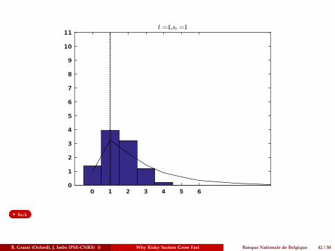
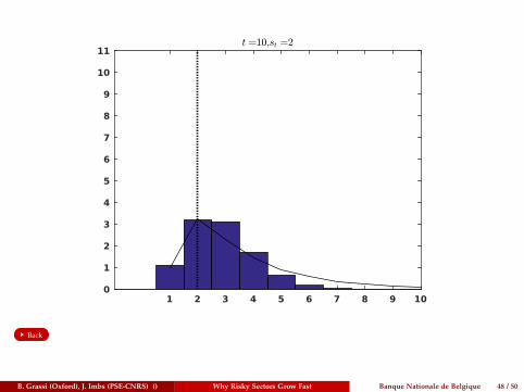
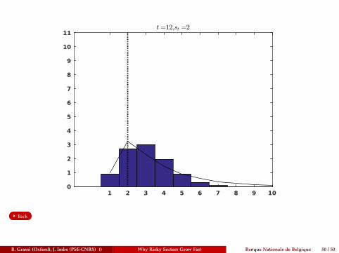
Productivity Distribution Dynamics
The productivity distribution is the sequence µt = {µs,t}s∈N∗
Exemple
B. Grassi (Oxford), J. Imbs (PSE-CNRS) () Why Risky Sectors Grow Fast Banque Nationale de Belgique 14 / 50

Productivity Distribution Dynamics
The productivity distribution is the sequence µt = {µs,t}s∈N∗
For s > st the evolution of the productivity distribution is
µs,t+1 = aµs+1,t + bµs,t + cµs−1,t + Stµs,t
N− St
◮ Contribution of experimenter firms
Exemple
B. Grassi (Oxford), J. Imbs (PSE-CNRS) () Why Risky Sectors Grow Fast Banque Nationale de Belgique 14 / 50

Productivity Distribution Dynamics
The productivity distribution is the sequence µt = {µs,t}s∈N∗
For s > st the evolution of the productivity distribution is
µs,t+1 = aµs+1,t + bµs,t + cµs−1,t + Stµs,t
N− St
◮ Contribution of experimenter firms◮ Contribution of the St imitators
and we have for s ∈ {st − 1, st}
µs,t+1 =
{aµst+1,t + bµst,t + St
µst,t
N−Stif s = st
aµst,t if s = st − 1
The minimum level at t+ 1 is st − 1:
∀s < st − 1, µs,t+1 = 0
Exemple
B. Grassi (Oxford), J. Imbs (PSE-CNRS) () Why Risky Sectors Grow Fast Banque Nationale de Belgique 14 / 50

Balanced Growth PathEquilibrium Concept
Aggregate output is the sum of firm level output:
Yt = ∑Ni=1 ϕsi,t = ∑
∞s=1 ϕsµs,t
B. Grassi (Oxford), J. Imbs (PSE-CNRS) () Why Risky Sectors Grow Fast Banque Nationale de Belgique 15 / 50

Balanced Growth PathEquilibrium Concept
Aggregate output is the sum of firm level output:
Yt = ∑Ni=1 ϕsi,t = ∑
∞s=1 ϕsµs,t
(Scale invariance) for g = ϕη , µt = {µs,t}s∈N scale invariant iffµs+ηt,t is identical for all t
A BGP is a equilibrium such that
i The sequence of productivity distribution and the growth rate, {µt, g}, arescale invariant.
ii Output grows geometricaly at rate g: Yt+1 = gYt
iii The minimum of the support of µt grows arithemticaly at rate η:st+1 = st + η where g = ϕη .
B. Grassi (Oxford), J. Imbs (PSE-CNRS) () Why Risky Sectors Grow Fast Banque Nationale de Belgique 15 / 50

Balanced Growth PathProductivity Distribution
Given g = ϕη with η > 0, the following satisfy the law of motion of theproductivity distribution:
µs,t =
0 for s < st−1
N(1− ϕ−δ)aϕ−δη for s = st−1 − 1
N(1− ϕ−δ)(1− cϕδ ϕ−δη
)for s = st−1
N(1− ϕ−δ)(
ϕs
ϕst−1
)−δfor s > st−1
B. Grassi (Oxford), J. Imbs (PSE-CNRS) () Why Risky Sectors Grow Fast Banque Nationale de Belgique 16 / 50

Balanced Growth PathProductivity Distribution
Given g = ϕη with η > 0, the following satisfy the law of motion of theproductivity distribution:
µs,t =
0 for s < st−1
N(1− ϕ−δ)aϕ−δη for s = st−1 − 1
N(1− ϕ−δ)(1− cϕδ ϕ−δη
)for s = st−1
N(1− ϕ−δ)(
ϕs
ϕst−1
)−δfor s > st−1
This distribution is Pareto above st with tail index δ =log a
clog ϕ
B. Grassi (Oxford), J. Imbs (PSE-CNRS) () Why Risky Sectors Grow Fast Banque Nationale de Belgique 16 / 50

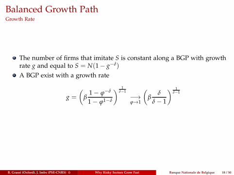
Balanced Growth PathGrowth Rate
The number of firms that imitate S is constant along a BGP with growthrate g and equal to S = N(1− g−δ)
B. Grassi (Oxford), J. Imbs (PSE-CNRS) () Why Risky Sectors Grow Fast Banque Nationale de Belgique 18 / 50

Balanced Growth PathGrowth Rate
The number of firms that imitate S is constant along a BGP with growthrate g and equal to S = N(1− g−δ)
A BGP exist with a growth rate
g =
(β1− ϕ−δ
1− ϕ1−δ
) 1δ−1
−→ϕ→1
(β
δ
δ − 1
) 1δ−1
B. Grassi (Oxford), J. Imbs (PSE-CNRS) () Why Risky Sectors Grow Fast Banque Nationale de Belgique 18 / 50

Balanced Growth PathGrowth Rate
The number of firms that imitate S is constant along a BGP with growthrate g and equal to S = N(1− g−δ)
A BGP exist with a growth rate
g =
(β1− ϕ−δ
1− ϕ1−δ
) 1δ−1
−→ϕ→1
(β
δ
δ − 1
) 1δ−1
The growth rate is decreasing in the tail index δ:
The fatter is the tail, the higher is the growth rate
B. Grassi (Oxford), J. Imbs (PSE-CNRS) () Why Risky Sectors Grow Fast Banque Nationale de Belgique 18 / 50

Aggregate Uncertainty from Micro Shocks
So far, we assumed that the law of large number always holds (as ifthere were a continuum of firms).
B. Grassi (Oxford), J. Imbs (PSE-CNRS) () Why Risky Sectors Grow Fast Banque Nationale de Belgique 20 / 50

Aggregate Uncertainty from Micro Shocks
So far, we assumed that the law of large number always holds (as ifthere were a continuum of firms).
However, we assumed a finite number of firms distributed according toa Pareto distribution.
B. Grassi (Oxford), J. Imbs (PSE-CNRS) () Why Risky Sectors Grow Fast Banque Nationale de Belgique 20 / 50
Aggregate Uncertainty from Micro Shocks
So far, we assumed that the law of large number always holds (as ifthere were a continuum of firms).
However, we assumed a finite number of firms distributed according toa Pareto distribution.
Gabaix (2011): If the distribution is fat tail ⇒ Aggregate Fluctuation.
B. Grassi (Oxford), J. Imbs (PSE-CNRS) () Why Risky Sectors Grow Fast Banque Nationale de Belgique 20 / 50

Aggregate Uncertainty from Micro Shocks
So far, we assumed that the law of large number always holds (as ifthere were a continuum of firms).
However, we assumed a finite number of firms distributed according toa Pareto distribution.
Gabaix (2011): If the distribution is fat tail ⇒ Aggregate Fluctuation.
Here we follow Carvalho and Grassi (2015) to account for the aggregatefluctuation arising from idiosyncratic shocks.
B. Grassi (Oxford), J. Imbs (PSE-CNRS) () Why Risky Sectors Grow Fast Banque Nationale de Belgique 20 / 50

Firm’s Problem under Aggregate Uncertainty
The firm problem is:
V(s, µt) = Max
{ϕs + βEt
[
∑s′V(s′, µt+1)Ps,s′
]; βEt
[
∑s′≥st
V(s′, µt+1)µs′,t
N− St
]}
B. Grassi (Oxford), J. Imbs (PSE-CNRS) () Why Risky Sectors Grow Fast Banque Nationale de Belgique 21 / 50

Firm’s Problem under Aggregate Uncertainty
The firm problem is:
V(s, µt) = Max
{ϕs + βEt
[
∑s′V(s′, µt+1)Ps,s′
]; βEt
[
∑s′≥st
V(s′, µt+1)µs′,t
N− St
]}
Which yields a threshold rule for st
{s < st, VI
t(s) > VEt (s) the firm decides to imitate
s ≥ st, VIt(s) ≤ VE
t (s) the firm decides to experiment
B. Grassi (Oxford), J. Imbs (PSE-CNRS) () Why Risky Sectors Grow Fast Banque Nationale de Belgique 21 / 50

Productivity Distribution Dynamics
���
��
�
��
���
�
������ ���
����
�
����
�����
�
��� ���
���
����
�
����
�����
�
��� ������
��
�
��
���
�
������
�������� � ���
������������ � ���
B. Grassi (Oxford), J. Imbs (PSE-CNRS) () Why Risky Sectors Grow Fast Banque Nationale de Belgique 22 / 50

Law of motion of the productivity distributionContinuum of firms
In the case of a continuum of firms we had:
µs,t+1 =
aµs+1,t + bµs,t + cµs−1,t + Stµs,t
N−Stif s > st
aµst+1,t + bµst,t + Stµst ,t
N−Stif s = st
aµst,t if s = st − 10 if s < st
B. Grassi (Oxford), J. Imbs (PSE-CNRS) () Why Risky Sectors Grow Fast Banque Nationale de Belgique 23 / 50

Law of motion of the productivity distributionFinite number of firms
In the case of a finite number of firms we have:
µs,t+1 =
aµs+1,t + bµs,t + cµs−1,t + Stµs,t
N−St+εs,t if s > st
aµst+1,t + bµst,t + Stµst ,t
N−St+εst,t if s = st
aµst,t+εst−1,t if s = st − 10 if s < st
where the variance-covariance structure of the {εs,t}s is a function of {µs,t}s.
B. Grassi (Oxford), J. Imbs (PSE-CNRS) () Why Risky Sectors Grow Fast Banque Nationale de Belgique 24 / 50

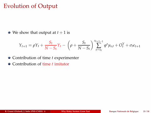
Evolution of Output
We show that output at t+ 1 is
Yt+1 = ρYt +St
N− StYt −
(ρ +
StN− St
) st+1−1
∑s=st
ϕsµs,t +OYt + σtǫt+1
B. Grassi (Oxford), J. Imbs (PSE-CNRS) () Why Risky Sectors Grow Fast Banque Nationale de Belgique 25 / 50

Evolution of Output
We show that output at t+ 1 is
Yt+1 = ρYt +St
N− StYt −
(ρ +
StN− St
) st+1−1
∑s=st
ϕsµs,t +OYt + σtǫt+1
Contribution of time t experimenter
B. Grassi (Oxford), J. Imbs (PSE-CNRS) () Why Risky Sectors Grow Fast Banque Nationale de Belgique 25 / 50
Evolution of Output
We show that output at t+ 1 is
Yt+1 = ρYt +St
N− StYt −
(ρ +
StN− St
) st+1−1
∑s=st
ϕsµs,t +OYt + σtǫt+1
Contribution of time t experimenter
Contribution of time t imitator
B. Grassi (Oxford), J. Imbs (PSE-CNRS) () Why Risky Sectors Grow Fast Banque Nationale de Belgique 25 / 50

Evolution of Output
We show that output at t+ 1 is
Yt+1 = ρYt +St
N− StYt −
(ρ +
StN− St
) st+1−1
∑s=st
ϕsµs,t +OYt + σtǫt+1
Contribution of time t experimenter
Contribution of time t imitator
Cost of time t+ 1 imitation
Aggregate shocks from idiosyncratic perturbation
B. Grassi (Oxford), J. Imbs (PSE-CNRS) () Why Risky Sectors Grow Fast Banque Nationale de Belgique 25 / 50

Evolution of Output
We can write the evolution of output growth as:
Yt+1
Yt= ρ
(∑
∞s=st+1
ϕsµs,t
Yt
)+
(St
N− St
)(∑
∞s=st+1
ϕsµs,t
Yt
)+
OYt
Yt+
σt
Ytǫt+1
B. Grassi (Oxford), J. Imbs (PSE-CNRS) () Why Risky Sectors Grow Fast Banque Nationale de Belgique 26 / 50

Evolution of Output
We can write the evolution of output growth as:
Yt+1
Yt= ρ
(∑
∞s=st+1
ϕsµs,t
Yt
)+
(St
N− St
)(∑
∞s=st+1
ϕsµs,t
Yt
)+
OYt
Yt+
σt
Ytǫt+1
Share of the output of the largest firms.
One over the ratio of small and large firms.
A persistence term: higher is the persistence if the output share of largefirms is important
A convergence term: if the number of small firms is high compare tothe number of large firms while the output share of the latter isimportant then growth will be higher.
B. Grassi (Oxford), J. Imbs (PSE-CNRS) () Why Risky Sectors Grow Fast Banque Nationale de Belgique 26 / 50

Aggregate Fluctuations
Aggregate uncertainty came from the term σtǫt+1 where:
σ2t
Y2t
= Vart
[Yt+1
Yt
]= ̺
∑s=st+1ϕ2sµs,t
Y2t
+ StVari∈Pt
[ϕsi,t ]
Y2t
+Oσ
t
Y2t
where Pt is the set of large firms (si,t > st+1) at t
B. Grassi (Oxford), J. Imbs (PSE-CNRS) () Why Risky Sectors Grow Fast Banque Nationale de Belgique 27 / 50

Aggregate Fluctuations
Aggregate uncertainty came from the term σtǫt+1 where:
σ2t
Y2t
= Vart
[Yt+1
Yt
]= ̺
∑s=st+1ϕ2sµs,t
Y2t
+ StVari∈Pt
[ϕsi,t ]
Y2t
+Oσ
t
Y2t
where Pt is the set of large firms (si,t > st+1) at t
A term similar to Carvalho and Grassi (2015)
An extra term due to imitation firms:
St
Y2t
Vari∈Pt[ϕsi,t ] =
StN− St
∑s=st+1ϕ2sµs,t
Y2t
− St(N− St)2
(∑s=st+1
ϕsµs,t
Yt
)2
Aggregate Fluctuations are driven by large firm-level dispersion:Larger is the dispersion among large firms, higher is the volatility ofoutput growth.
B. Grassi (Oxford), J. Imbs (PSE-CNRS) () Why Risky Sectors Grow Fast Banque Nationale de Belgique 27 / 50

Estimations: Growth
gyi,t = βi + γt + β1∑
Nts>τ yi,s,t
Yi,t+ β2
Si,t
Ni,t − Si,t· ∑
Nti>τ yi,s,t
Yi,t+
σi,t
Yi,tǫi,t
Fixed sector effects, year effects, heteroscedasticity.
τ = 500, 1000, or 2500 employees
B. Grassi (Oxford), J. Imbs (PSE-CNRS) Why Risky Sectors Grow Fast Banque Nationale de Belgique 1 / 4

Estimations: Growth (cont.)
Growth rates computed as Davis, Haltiwanger, and Schuh (1996) foreach sector i:
gyi,t =Yi,t − Yi,t−1
0.5 (Yi,t + Yi,t−1)
gyi,t computed for employment, sales, wages - from NBER CESManufacturing data. Use 5-year averages.
τ, Si,t, Ni,t, ∑Nts>τ yi,s,t, either sales or employment - all from Compustat.
Compute for 6, 5, 4, 3, and 2 NAICS digits. (Price deflators for sales onlyavailable form 4 digits)
Truncation innocuous if Pareto.
B. Grassi (Oxford), J. Imbs (PSE-CNRS) Why Risky Sectors Grow Fast Banque Nationale de Belgique 2 / 4

Table 1: Growth: threshold 1000 employees
Panel A: naics 6 digits
(1) (2) (3) (4) (5) (6)
VARIABLES sales sales empl. empl. wage wage
ratio sum sale big1000 sale -0.0102 -0.0133 -0.0014 -0.0012 0.0014*** 0.0013***
(0.0096) (0.0101) (0.0015) (0.0013) (0.0002) (0.0002)
interaction sale 1000 0.0195** 0.0229** 0.0004 -0.0008 0.0016*** 0.0017***
(0.0087) (0.0104) (0.0025) (0.0024) (0.0005) (0.0005)
ratio small big big1000 -0.0062 0.0062 -0.0005
(0.0061) (0.0042) (0.0012)
Observations 1,021 1,021 1,021 1,021 1,021 1,021
R-squared 0.0271 0.0288 0.0028 0.0065 0.0462 0.0465
Number of sector 114 114 114 114 114 114
Time FE YES YES YES YES YES YES
Sector FE YES YES YES YES YES YES
Panel B: naics 5 digits
(1) (2) (3) (4) (5) (6)
VARIABLES sales sales empl. empl. wage wage
ratio sum sale big1000 sale -0.0145 -0.0161 -0.0004 -0.0004 0.0014*** 0.0013***
(0.0124) (0.0134) (0.0005) (0.0004) (0.0001) (0.0001)
interaction sale 1000 0.0311 0.0341 -0.0002 -0.0005 0.0021*** 0.0022***
(0.0194) (0.0214) (0.0016) (0.0014) (0.0004) (0.0004)
ratio small big big1000 -0.0048 0.0023 -0.0005
(0.0055) (0.0046) (0.0011)
Observations 778 778 778 778 778 778
R-squared 0.0375 0.0386 0.0020 0.0026 0.0781 0.0783
Number of sector 87 87 87 87 87 87
Time FE YES YES YES YES YES YES
Sector FE YES YES YES YES YES YES
Panel C: naics 4 digits
(1) (2) (3) (4) (5) (6)
VARIABLES sales sales empl. empl. wage wage
ratio sum sale big1000 sale 0.0393 0.0251 -0.0128 -0.0139 0.0102 0.0108
(0.0446) (0.0425) (0.0083) (0.0086) (0.0086) (0.0090)
interaction sale 1000 0.0447 0.0608** 0.0042 0.0060 0.0023 0.0013
(0.0269) (0.0304) (0.0085) (0.0092) (0.0030) (0.0035)
ratio small big big1000 -0.0216 -0.0045 0.0024
(0.0149) (0.0062) (0.0031)
Observations 554 554 554 554 554 554
R-squared 0.0754 0.0872 0.0131 0.0143 0.0996 0.1020
Number of sector 62 62 62 62 62 62
Time FE YES YES YES YES YES YES
Sector FE YES YES YES YES YES YES
Robust standard errors in parentheses: *** p<0.01, ** p<0.05, * p<0.1
Note:
1

Table 2: Growth: threshold 500 employees
Panel A: naics 6 digits
(1) (2) (3) (4) (5) (6)
VARIABLES sales sales empl. empl. wage wage
ratio sum sale big500 sale -0.0099 -0.0120 -0.0016 -0.0013 0.0014*** 0.0013***
(0.0101) (0.0107) (0.0016) (0.0014) (0.0002) (0.0002)
interaction sale 500 0.0240** 0.0272* 0.0014 -0.0001 0.0019*** 0.0021***
(0.0113) (0.0139) (0.0032) (0.0028) (0.0004) (0.0004)
ratio small big big500 -0.0064 0.0101 -0.0012
(0.0117) (0.0079) (0.0015)
Observations 1,024 1,024 1,024 1,024 1,024 1,024
R-squared 0.0257 0.0266 0.0035 0.0084 0.0473 0.0479
Number of sector 114 114 114 114 114 114
Time FE YES YES YES YES YES YES
Sector FE YES YES YES YES YES YES
Panel B: naics 5 digits
(1) (2) (3) (4) (5) (6)
VARIABLES sales sales empl. empl. wage wage
ratio sum sale big500 sale -0.0117 -0.0111 -0.0004 -0.0004 0.0014*** 0.0014***
(0.0119) (0.0123) (0.0005) (0.0005) (0.0001) (0.0001)
interaction sale 500 0.0295 0.0281 -0.0002 -0.0003 0.0022*** 0.0021***
(0.0191) (0.0215) (0.0016) (0.0013) (0.0004) (0.0004)
ratio small big big500 0.0023 0.0007 0.0014
(0.0091) (0.0088) (0.0019)
Observations 781 781 781 781 781 781
R-squared 0.0246 0.0247 0.0022 0.0022 0.0773 0.0781
Number of sector 87 87 87 87 87 87
Time FE YES YES YES YES YES YES
Sector FE YES YES YES YES YES YES
Panel C: naics 4 digits
(1) (2) (3) (4) (5) (6)
VARIABLES sales sales empl. empl. wage wage
ratio sum sale big500 sale 0.0493 0.0417 -0.0150* -0.0162* 0.0109 0.0116
(0.0477) (0.0460) (0.0085) (0.0088) (0.0091) (0.0095)
interaction sale 500 0.0507 0.0639 0.0090 0.0116 0.0015 0.0001
(0.0334) (0.0385) (0.0101) (0.0107) (0.0042) (0.0050)
ratio small big big500 -0.0180 -0.0067 0.0037
(0.0176) (0.0098) (0.0052)
Observations 557 557 557 557 557 557
R-squared 0.0640 0.0683 0.0177 0.0191 0.0970 0.0999
Number of sector 62 62 62 62 62 62
Time FE YES YES YES YES YES YES
Sector FE YES YES YES YES YES YES
Robust standard errors in parentheses: *** p<0.01, ** p<0.05, * p<0.1
Note:
2

Table 3: Growth: threshold 2500 employees
Panel A: naics 6 digits
v (1) (2) (3) (4) (5) (6)
VARIABLES sales sales empl. empl. wage wage
ratio sum sale big2500 sale -0.0125 -0.0130 -0.0010 -0.0007 0.0014*** 0.0014***
(0.0099) (0.0106) (0.0012) (0.0010) (0.0002) (0.0002)
interaction sale 2500 0.0157** 0.0161** -0.0012 -0.0023 0.0010* 0.0011*
(0.0070) (0.0081) (0.0020) (0.0022) (0.0006) (0.0006)
ratio small big big2500 -0.0006 0.0045** -0.0002
(0.0035) (0.0021) (0.0011)
Observations 1,000 1,000 1,000 1,000 1,000 1,000
R-squared 0.0324 0.0324 0.0038 0.0101 0.0422 0.0423
Number of sector 114 114 114 114 114 114
Time FE YES YES YES YES YES YES
Sector FE YES YES YES YES YES YES
Panel B: naics 5 digits
v (1) (2) (3) (4) (5) (6)
VARIABLES sales sales empl. empl. wage wage
ratio sum sale big2500 sale -0.0135 -0.0134 -0.0003 -0.0002 0.0013*** 0.0013***
(0.0124) (0.0130) (0.0004) (0.0003) (0.0002) (0.0001)
interaction sale 2500 0.0256 0.0255 -0.0008 -0.0011 0.0021*** 0.0021***
(0.0156) (0.0171) (0.0015) (0.0014) (0.0005) (0.0004)
ratio small big big2500 0.0002 0.0014 -0.0001
(0.0030) (0.0017) (0.0006)
Observations 763 763 763 763 763 763
R-squared 0.0486 0.0486 0.0026 0.0035 0.0814 0.0815
Number of sector 87 87 87 87 87 87
Time FE YES YES YES YES YES YES
Sector FE YES YES YES YES YES YES
Panel C: naics 4 digits
v (1) (2) (3) (4) (5) (6)
VARIABLES sales sales empl. empl. wage wage
ratio sum sale big2500 sale 0.0264 -0.0040 -0.0092 -0.0125 0.0102 0.0109
(0.0418) (0.0410) (0.0079) (0.0083) (0.0087) (0.0088)
interaction sale 2500 0.0409** 0.0571** -0.0001 0.0033 0.0018 0.0010
(0.0204) (0.0224) (0.0068) (0.0074) (0.0022) (0.0024)
ratio small big big2500 -0.0191* -0.0072 0.0016
(0.0097) (0.0050) (0.0019)
Observations 549 549 549 549 549 549
R-squared 0.0999 0.1267 0.0096 0.0191 0.1018 0.1050
Number of sector 62 62 62 62 62 62
Time FE YES YES YES YES YES YES
Sector FE YES YES YES YES YES YES
Robust standard errors in parentheses: *** p<0.01, ** p<0.05, * p<0.1
Note:
3

Estimations: Volatility
VAR (gyi,t) = αi + γt + α1∑
Nts>τ (yi,s,t)
2
(Yi,t)2
+ α2Si,t
Ni,t − Si,t· ∑
Nts>τ (yi,s,t)
2
(Yi,t)2
+ ηi,t
Fixed sector effects, year effects,
τ = 500, 1000, or 2500 employees
B. Grassi (Oxford), J. Imbs (PSE-CNRS) Why Risky Sectors Grow Fast Banque Nationale de Belgique 3 / 4

Estimations: Volatility (cont.)
Volatility computed as Carvalho and Gabaix (1996) for each sector i:
VAR (gyi,t) = 2
√π
2|εi,t|
whereYi,t − Yi,t−1 = ρ (Yi,t−1 − Yi,t−2) + εi,t
Smoothed with HP filter.
VAR (gyi,t)computed for employment and sales - from NBER CESManufacturing data.
τ, Si,t, Ni,t, ∑Nts>τ yi,s,t, either sales or employment - all from Compustat.
Compute for 6, 5, 4, 3, and 2 NAICS digits. (Price deflators for sales onlyavailable form 4 digits)
B. Grassi (Oxford), J. Imbs (PSE-CNRS) Why Risky Sectors Grow Fast Banque Nationale de Belgique 4 / 4
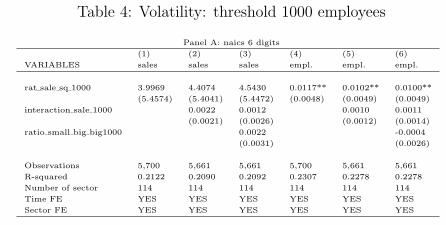
Table 4: Volatility: threshold 1000 employees
Panel A: naics 6 digits
(1) (2) (3) (4) (5) (6)
VARIABLES sales sales sales empl. empl. empl.
rat sale sq 1000 3.9969 4.4074 4.5430 0.0117** 0.0102** 0.0100**
(5.4574) (5.4041) (5.4472) (0.0048) (0.0049) (0.0049)
interaction sale 1000 0.0022 0.0012 0.0010 0.0011
(0.0021) (0.0026) (0.0012) (0.0014)
ratio small big big1000 0.0022 -0.0004
(0.0031) (0.0026)
Observations 5,700 5,661 5,661 5,700 5,661 5,661
R-squared 0.2122 0.2090 0.2092 0.2307 0.2278 0.2278
Number of sector 114 114 114 114 114 114
Time FE YES YES YES YES YES YES
Sector FE YES YES YES YES YES YES
Panel B: naics 5 digits
(1) (2) (3) (4) (5) (6)
VARIABLES sales sales sales empl. empl. empl.
rat sale sq 1000 -1.0263 -0.6162 -0.7143 0.0080*** 0.0060*** 0.0058**
(12.3048) (13.2670) (13.3113) (0.0008) (0.0022) (0.0024)
interaction sale 1000 0.0044 0.0050 0.0011 0.0012
(0.0050) (0.0054) (0.0014) (0.0015)
ratio small big big1000 -0.0012 -0.0009
(0.0038) (0.0028)
Observations 4,350 4,316 4,316 4,350 4,316 4,316
R-squared 0.2629 0.2604 0.2604 0.2648 0.2622 0.2623
Number of sector 87 87 87 87 87 87
Time FE YES YES YES YES YES YES
Sector FE YES YES YES YES YES YES
Panel C: naics 4 digits
(1) (2) (3) (4) (5) (6)
VARIABLES sales sales sales empl. empl. empl.
rat sale sq 1000 6.9489*** 10.3087*** 10.2819*** 0.0948** -0.0012 -0.0211
(1.0216) (2.9942) (3.0225) (0.0436) (0.0776) (0.0887)
interaction sale 1000 0.0101 0.0113 0.0066 0.0083
(0.0079) (0.0091) (0.0046) (0.0057)
ratio small big big1000 -0.0019 -0.0045
(0.0056) (0.0041)
Observations 3,100 3,079 3,079 3,100 3,079 3,079
R-squared 0.3098 0.3128 0.3129 0.2902 0.3000 0.3015
Number of sector 62 62 62 62 62 62
Time FE YES YES YES YES YES YES
Sector FE YES YES YES YES YES YES
Robust standard errors in parentheses: *** p<0.01, ** p<0.05, * p<0.1
Note:
4

Table 5: Volatility: threshold 500 employees
Panel A: naics 6 digits
(1) (2) (3) (4) (5) (6)
VARIABLES sales sales sales empl. empl. empl.
rat sale sq 500 4.2360 4.5794 4.7693 0.0118** 0.0107** 0.0112**
(5.3632) (5.2944) (5.3398) (0.0049) (0.0049) (0.0049)
interaction sale 500 0.0027 0.0011 0.0007 0.0004
(0.0034) (0.0040) (0.0012) (0.0012)
ratio small big big500 0.0040 0.0020
(0.0062) (0.0040)
Observations 5,700 5,685 5,685 5,700 5,685 5,685
R-squared 0.2125 0.2131 0.2135 0.2308 0.2314 0.2316
Number of sector 114 114 114 114 114 114
Time FE YES YES YES YES YES YES
Sector FE YES YES YES YES YES YES
Panel B: naics 5 digits
(1) (2) (3) (4) (5) (6)
VARIABLES sales sales sales empl. empl. empl.
rat sale sq 500 -0.9234 -0.8901 -0.8802 0.0080*** 0.0066*** 0.0066***
(12.2355) (13.0980) (13.1477) (0.0008) (0.0018) (0.0019)
interaction sale 500 0.0047 0.0046 0.0008 0.0008
(0.0058) (0.0061) (0.0012) (0.0012)
ratio small big big500 0.0002 0.0003
(0.0059) (0.0039)
Observations 4,350 4,335 4,335 4,350 4,335 4,335
R-squared 0.2629 0.2635 0.2635 0.2648 0.2647 0.2647
Number of sector 87 87 87 87 87 87
Time FE YES YES YES YES YES YES
Sector FE YES YES YES YES YES YES
Panel C: naics 4 digits
(1) (2) (3) (4) (5) (6)
VARIABLES sales sales sales empl. empl. empl.
rat sale sq 500 6.9494*** 10.2968*** 10.2849*** 0.0960** -0.0087 -0.0123
(1.0270) (2.7478) (2.7182) (0.0425) (0.0813) (0.0937)
interaction sale 500 0.0165 0.0150 0.0082 0.0085
(0.0116) (0.0130) (0.0058) (0.0071)
ratio small big big500 0.0022 -0.0010
(0.0092) (0.0058)
Observations 3,100 3,090 3,090 3,100 3,090 3,090
R-squared 0.3098 0.3152 0.3153 0.2903 0.2983 0.2984
Number of sector 62 62 62 62 62 62
Time FE YES YES YES YES YES YES
Sector FE YES YES YES YES YES YES
Robust standard errors in parentheses: *** p<0.01, ** p<0.05, * p<0.1
Note:
5

Table 6: Volatility: threshold 2500 employees
Panel A: naics 6 digits
(1) (2) (3) (4) (5) (6)
VARIABLES sales sales sales empl. empl. empl.
rat sale sq 2500 3.7020 4.0270 4.2546 0.0116** 0.0080* 0.0084*
(5.8313) (5.7504) (5.7985) (0.0050) (0.0044) (0.0044)
interaction sale 2500 0.0020 0.0011 0.0021* 0.0019
(0.0014) (0.0017) (0.0012) (0.0012)
ratio small big big2500 0.0021 0.0008
(0.0019) (0.0014)
Observations 5,700 5,491 5,491 5,700 5,491 5,491
R-squared 0.2117 0.1971 0.1978 0.2303 0.2229 0.2231
Number of sector 114 114 114 114 114 114
Time FE YES YES YES YES YES YES
Sector FE YES YES YES YES YES YES
Panel B: naics 5 digits
(1) (2) (3) (4) (5) (6)
VARIABLES sales sales sales empl. empl. empl.
rat sale sq 2500 -1.3564 -1.4694 -1.4611 0.0080*** 0.0049* 0.0049*
(12.8788) (14.0371) (14.0775) (0.0008) (0.0028) (0.0029)
interaction sale 2500 0.0035 0.0035 0.0017 0.0017
(0.0040) (0.0042) (0.0016) (0.0016)
ratio small big big2500 0.0001 0.0001
(0.0019) (0.0013)
Observations 4,350 4,195 4,195 4,350 4,195 4,195
R-squared 0.2629 0.2547 0.2547 0.2648 0.2615 0.2615
Number of sector 87 87 87 87 87 87
Time FE YES YES YES YES YES YES
Sector FE YES YES YES YES YES YES
Panel C: naics 4 digits
(1) (2) (3) (4) (5) (6)
VARIABLES sales sales sales empl. empl. empl.
rat sale sq 2500 7.1457*** 10.6360*** 10.6491*** 0.0918** 0.0041 -0.0081
(1.0963) (3.6049) (3.5823) (0.0451) (0.0629) (0.0695)
interaction sale 2500 0.0066 0.0061 0.0058* 0.0063*
(0.0062) (0.0063) (0.0033) (0.0037)
ratio small big big2500 0.0008 -0.0014
(0.0027) (0.0018)
Observations 3,100 3,037 3,037 3,100 3,037 3,037
R-squared 0.3098 0.3068 0.3068 0.2902 0.3001 0.3006
Number of sector 62 62 62 62 62 62
Time FE YES YES YES YES YES YES
Sector FE YES YES YES YES YES YES
Robust standard errors in parentheses: *** p<0.01, ** p<0.05, * p<0.1
Note:
6

Table 4: Volatility: threshold 1000 employees
Panel A: naics 6 digits
(1) (2) (3) (4) (5) (6)
VARIABLES sales sales sales empl. empl. empl.
rat sale sq 1000 3.9969 4.4074 4.5430 0.0117** 0.0102** 0.0100**
(5.4574) (5.4041) (5.4472) (0.0048) (0.0049) (0.0049)
interaction sale 1000 0.0022 0.0012 0.0010 0.0011
(0.0021) (0.0026) (0.0012) (0.0014)
ratio small big big1000 0.0022 -0.0004
(0.0031) (0.0026)
Observations 5,700 5,661 5,661 5,700 5,661 5,661
R-squared 0.2122 0.2090 0.2092 0.2307 0.2278 0.2278
Number of sector 114 114 114 114 114 114
Time FE YES YES YES YES YES YES
Sector FE YES YES YES YES YES YES
Panel B: naics 5 digits
(1) (2) (3) (4) (5) (6)
VARIABLES sales sales sales empl. empl. empl.
rat sale sq 1000 -1.0263 -0.6162 -0.7143 0.0080*** 0.0060*** 0.0058**
(12.3048) (13.2670) (13.3113) (0.0008) (0.0022) (0.0024)
interaction sale 1000 0.0044 0.0050 0.0011 0.0012
(0.0050) (0.0054) (0.0014) (0.0015)
ratio small big big1000 -0.0012 -0.0009
(0.0038) (0.0028)
Observations 4,350 4,316 4,316 4,350 4,316 4,316
R-squared 0.2629 0.2604 0.2604 0.2648 0.2622 0.2623
Number of sector 87 87 87 87 87 87
Time FE YES YES YES YES YES YES
Sector FE YES YES YES YES YES YES
Panel C: naics 4 digits
(1) (2) (3) (4) (5) (6)
VARIABLES sales sales sales empl. empl. empl.
rat sale sq 1000 6.9489*** 10.3087*** 10.2819*** 0.0948** -0.0012 -0.0211
(1.0216) (2.9942) (3.0225) (0.0436) (0.0776) (0.0887)
interaction sale 1000 0.0101 0.0113 0.0066 0.0083
(0.0079) (0.0091) (0.0046) (0.0057)
ratio small big big1000 -0.0019 -0.0045
(0.0056) (0.0041)
Observations 3,100 3,079 3,079 3,100 3,079 3,079
R-squared 0.3098 0.3128 0.3129 0.2902 0.3000 0.3015
Number of sector 62 62 62 62 62 62
Time FE YES YES YES YES YES YES
Sector FE YES YES YES YES YES YES
Robust standard errors in parentheses: *** p<0.01, ** p<0.05, * p<0.1
Note:
4

Conclusion
Presented a model of idea flows with growth and volatility
Growth and volatility depend (non linearly) on relative size of largefirms, and on relative numbers of small firms.
Predictions borne out in US sector data: growth and volatility correlatewith firm distribution – i.e. reflect risk taking behavior of firms in agiven sector.
Relation weakens with aggregation – consistent with productivity-basedexplanation.
B. Grassi (Oxford), J. Imbs (PSE-CNRS) () Why Risky Sectors Grow Fast Banque Nationale de Belgique 37 / 50

Back
B. Grassi (Oxford), J. Imbs (PSE-CNRS) () Why Risky Sectors Grow Fast Banque Nationale de Belgique 38 / 50

Back
B. Grassi (Oxford), J. Imbs (PSE-CNRS) () Why Risky Sectors Grow Fast Banque Nationale de Belgique 39 / 50

Back
B. Grassi (Oxford), J. Imbs (PSE-CNRS) () Why Risky Sectors Grow Fast Banque Nationale de Belgique 40 / 50

Back
B. Grassi (Oxford), J. Imbs (PSE-CNRS) () Why Risky Sectors Grow Fast Banque Nationale de Belgique 41 / 50
Back
B. Grassi (Oxford), J. Imbs (PSE-CNRS) () Why Risky Sectors Grow Fast Banque Nationale de Belgique 42 / 50

Back
B. Grassi (Oxford), J. Imbs (PSE-CNRS) () Why Risky Sectors Grow Fast Banque Nationale de Belgique 43 / 50

Back
B. Grassi (Oxford), J. Imbs (PSE-CNRS) () Why Risky Sectors Grow Fast Banque Nationale de Belgique 44 / 50

Back
B. Grassi (Oxford), J. Imbs (PSE-CNRS) () Why Risky Sectors Grow Fast Banque Nationale de Belgique 45 / 50

Back
B. Grassi (Oxford), J. Imbs (PSE-CNRS) () Why Risky Sectors Grow Fast Banque Nationale de Belgique 46 / 50

Back
B. Grassi (Oxford), J. Imbs (PSE-CNRS) () Why Risky Sectors Grow Fast Banque Nationale de Belgique 47 / 50
Back
B. Grassi (Oxford), J. Imbs (PSE-CNRS) () Why Risky Sectors Grow Fast Banque Nationale de Belgique 48 / 50

Back
B. Grassi (Oxford), J. Imbs (PSE-CNRS) () Why Risky Sectors Grow Fast Banque Nationale de Belgique 49 / 50
Back
B. Grassi (Oxford), J. Imbs (PSE-CNRS) () Why Risky Sectors Grow Fast Banque Nationale de Belgique 50 / 50