why are american presidential election campaign polls …gking.harvard.edu/files/bj215.pdf · why...

B. J . Pol. S. 23,40945 1 Printed in Great Britain

Copyright O 1993 Cambridge University Press

Why Are American Presidential Election Campaign Polls So Variable When Votes Are So Predictable? A N D R E W G E L M A N A N D G A R Y K I N G *

As most political scientists know, the outcome of the American presidential election can be predicted within a few percentage points (in the popular vote), based on information available months before the election. Thus, the general campaign for president seems irrelevant to the outcome (except in very close elections), despite all the media coverage of campaign strategy. However, it is also well known that the pre-election opinion polls can vary wildly over the campaign, and this variation is generally attributed to events in the campaign. How can campaign events affect people's opinions on whom they plan to vote for, and yet not affect the outcome of the election? For that matter, why do voters consistently increase their rupport for a candidate during his nominating convention, even though the conventions are almost entirely predictable events whose effects can be rationally forecast?

In this exploratory study, we consider several intuitively appealing, but ultimately wrong. resolutions to this puzzle and discuss our current understanding of what causes opinion polls to fluctuate while reaching a predictable outcome. Our evidence is based on graphical presentation and analysis of over 67,000 individual-level responses from forty-nine commercial polls during the 1988 campaign and many other aggregate poll results from the 1952-92campaigns.

We show that responses to pollsters during the campaign are not generally informed or even, in a sense we describe, 'rational'. In contrast, voters decide, based on their enlightened preferences, as formed by the information they have learned during the campaign, as wel! as basic political cues such as ideology and party identification, which candidate to support eventually. We cannot prove this conclusion, but we do show that it is consistent with the aggregate forecasts and individual-level opinion poll responses. Based on the enlightened preferences hypothesis, we conclude that the news media have an important effect on the outcome of presidential elections - not through misleading advertisements. sound bites, or spin doctors, but rather by conveying candidates' positions on important issues.

Something is amiss in the scholarly study of American presidential elections. For some time now, political scientists have forecast the outcome of presidential elections accurately using only information available before the start of the general election campaign. However, the numerous 'trial heat' public opinion surveys (polls about whether likely voters plan to cast their ballots for the Democratic or Republican candidate for president) conducted during the campaign vary enormously in support for the Democratic and Republican

* Gelman, Department of Statistics, University of California, Berkeley; King. Department of Government, Harvard University. We thank Eric Oliver and Maggie Trevor for research assistance, and Larry Bartels, Neal Beck, Tom Belin. M o Fiorina, John Kessel, Mik Laver, Eileen McDonaugh, Phil Paolino, Keith Poole, Doug Price, Phillip Price. Sid Verba and D. Stephen Voss for helpful comments, and the National Science Foundation for a research grant. All graphs were made using the S system. This is a revised version of a paper which received the Pi Sigma Alpha award for the best paper at the annual meeting of the Midwest Political Science Association, Chicago. 1992.

candidates. At one point during the 1988 general election campaign, survey respondents favoured Dukakis over Bush by 17 percentage points, and yet any reasonable application of the political science literature would have made George Bush almost certain to win the November election.

In addition to being interesting in its own right, the puzzle stated in the title of this article is important for three related reasons. First, given our profession's heavy reliance on public opinion surveys for studying presidential elections and numerous other phenomena, the puzzle represents a large void in our substantive understanding and possibly also a very serious methodological problem for much existing research outside this area. The existence of the puzzle means that we cannot rely on answers to at least some survey questions. What political science obviously needs is a very clear broader theory of the survey response, so that we can decide which questions contain directly useful information. Although there has been much interesting work on the subject, we certainly have no fully satisfactory theory yet.' This is not a problem we solve in this article, but any resolution of the more general problem must also account for our puzzle.

A second reason for studying this subject is its potential contribution to what political philosophers have called 'the epistemological problem of interests: how we can know what they are.'' Dahl defines 'interests' by appealing to the concept of enlightened understanding: 'A person's interest or good is whatever that person would choose with fullest attainable understanding of the experience resulting from that choice and its most relevant alternatives.' He and others have asked, 'What processes or institutions can best be counted on to protect these interests?' We have no final answer to this question, but the issues we address and evidence we provide may help to focus the question more precisely.

Finally, the puzzle has a practical consequence, since mainstream journalists respond to it largely by ignoring the lessons of political science and instead interpreting each short-term change in the public opinion polls as a serious change in the likely fortunes of the candidates. This focus is in part responsible for the relatively issue-free, or 'horse race', aspect of presidential campaign media coverage, which at its most extreme finds journalists interpreting the race by deconstructing the claims of competing 'spin doctors'. Conversely,

' Christopher Achen, 'Mass Political Attitudes and the Survey Response', American Political Science Review, 69 (1975), 1218-23; Stanley Feldman, 'What Do Survey Questions Really Measure?' Political Methodologist, 4 (1991), 8-12; T. Piazza, Paul Sniderman and Phillip Tetlock, 'Analysis of the Dynamics of Political Reasoning: A General-Purpose Computer Assisted Methodology', Political Analysis, 1 (1989), 99-120. ' Robert Dahl, Democracy and Its Critics (New Haven, Conn.: Yale University Press, 1989),

p. 181.

Why Are Presidental Election Polls So Variable? 41 1

some political observers, noting the success of forecasters in predicting elections months ahead of time, hold that the general election campaign has no effect on the outcome of the presidential election. Neither of these extreme positions fully captures the truth; at the end of this article, we return to a discussion of the roie of the media in election campaigns.

As far as we know, the arguments and evidence in this paper apply only to the general election campaign for the American President (see Section 2.2). Sorting out where it applies, and why, is an important topic for future research. In Section 1, we review the evidence regarding political scientists' forecasts and the variability of poll results. Underlying our ability to forecast is the profession's distinctive model of voter decision making. Section 2 discusses this model, as well as the alternative model implicitly followed by most accounts of the election in the news media. We work our way through several plausible, but flawed, explanations for this puzzle in Section 3. We are far from a final answer to our puzzle, but we do have one tentative explanation, which is consistent with all our existing evidence. We outline this hypothesis in Section 4 and present the evidence for it in Section 5. We conclude in Section 6 with a discussion of the implications for the role of the media in presidential election campaigns.

Our intended contribution in this article is to raise the question in our title and provide evidence sufficient to dismiss many apparently reasonable and 'obvious' hypotheses (including our own prior beliefs). Because of the largely exploratory nature of relevant existing theories, we make extensive use of graphical techniques. This enables us to evaluate a series of specific hypotheses while still not obscuring features of the data that might suggest novel approaches or new hypotheses.

1. F O R E C A S T I N G E V I D E N C E A N D D A T A S U M M A R I E S

Rosenstone's forecasting model is one of the most developed and successful of the recent contributions to the literature, and it is the empirical results of this model on which we focus.' His model is based on measurable economic and political variables that were discovered and analysed by numerous researchers over many decades, and not on trial heat polls. Even if one were to disagree with the particulars of Rosenstone's model, it would be hard to

Steven J. Rosenstone, Forecasting Presidential Elections (New Haven, Conn.: Yale University Press, 1983).

412 G E L M A N A N D K I N G

deny that past presidential elections have been forecast fairly accurately using these method^.^

1.1. Political Science Forecasts up to 1988

Rosenstone summarizes his considerable success at forecasting presidential elections through 1980. Perhaps even stronger evidence is that his model has continued to forecast very well in the two elections since the publication of his book, as recounted by ~osenstone. ' In both 1984 and 1988, Rosenstone's forecasts fell within 1 per cent of the nationwide popular vote and predicted only a few states incorrectly, an excellent performance, considering that the forecasts were made months before the election. Table 1 summarizes the performance of Rosenstone's model, along with our forecasts for 1992 (see below), by com- paring forecasts made at the start of the general election campaign with those from the national polls, media prognoses and judgements by political strategists taken at the same time.

Rosenstone also presents what he calls 'perfect information forecasts', based on information theoretically, but not actually, available before the election, such as late changes in real disposable income. (This would be actually available if the government released this information earlier.) These perfect information forecasts are generally significant improvements. They are obviously of less use for actual forecasting, but they confirm the most important general point from our perspective: the outcomes of recent elections can be predicted within a few percentage points in the popular vote, based on events that have occurred before Labor Day (the first Monday in September).

Other forecasting models, also based on economic and political variables measured before the start of the campaign, have performed well, and often

Michael S. Lewis-Beck, 'Election Forecasts in 1984: How Accurate Were They?' PS, 18 (1985), 53-62, and Michael S. Lewis-Beck and Tom W. Rice, Forecasting Elections (Washington, DC: Congressional Quarterly Press, 1992) review many other statistical forecasting models. Allan J. Lichtman and Ken DeCell, The Thirteen Keys to the Presidency (Lanham, NY: Madison Books, 1990) and Robert Forsythe, Forrest Nelson, George Neumann and Jack Wright, 'The Iowa Presi- dential Stock Market: A Field Experiment', Research in Experimental Economics, 4 (1991), 1113, present some non-statistical approaches to forecasting presidential elections. Social scientists have been explaining and forecasting Individual votes and aggregate election outcomes almost since the start of the discipline. The first quantitative article published in a political science journal (about political science) was on voting behaviour (William Ogburn and Inez Goltra, 'How Women Vote: A Study of an Election in Portland, Oregon', Political Science Quarterly, 34 (1919), 413-33), and voting, particularly in presidential elections, has almost always remained a lively area of research.

' Steven J. Rosenstone, 'Predicting Elections' (Ann Arbor: University of Michigan, unpublished manuscript, 1990). In Forecasting Presidential Elections, p. 122, Rosenstone also reports sending letters on 14 October 1980 to twenty scholars with his forecasts of the November 1980 election.


T A B L E 1 Presidential Election Forecasting Errors

Forecasts Errors

1984 National Popular Vote Rosenstone 0.3 percent National polls (average miss) 5.3 percent

National Electoral Vote Rosenstone 48 electoral votes Media prognoses (average miss) 129 electoral votes Political strategists (average miss) 1 15 electoral votes

1988 National Popular Vote Rosenstone National polls (average miss)

National Electoral Vote Rosenstone Media prognoses (average miss)

0.2 percent 2.8 percent

82 electoral votes 13 1 electoral votes

1992 National Popular Vote Gelman and King 0.3 percent National polls, early September (average miss) 2.8 percent National polls, mid-October (average miss) 5.4 percent

National Electoral Vote Gelman and King 5.6 electoral votes State polls, September 59 electoral votes

Nore: All popular vote forecasts are expressed in terms of the Democratic candidate's share of the two-party vote. The 1984 forecasts were made in mid-July; the 1988 forecasts were made in early September; the 1992 forecasts were performed in early-October, but only used information available in early September. When the media declared states as 'toss-ups', the electoral votes were divided evenly between the two major parties and states were counted as half a miss.

Sourcefor 1984 and 1988forecasts: Rosenstone. 'Predicting Elections'. Tables 1 and 2.

better, in recent years6 By contrast, public opinion polls at this time gave relatively useless forecasts of the election outcome. The predictions of media experts and political strategists were not much better.?

See, for example, Ian Budge and Dennis Farlie, Voting and Parry Comperition (New York: Wiley, 1977); Edward R. Tufte, Political Conrrol ofrhe Economy (Princeton, N J : Princeton Univer- sity Press, 1978); Ray C. Fair, 'The Effect of Economic Events on Votes for President', Review of Economics and Sratistics, 60 (1978), 159-73: and 'The Effect of Economic Events on Votes for President: 1980 Update'. Review ofEconomics and Srarisrics, 64 (1982), 322-5; and 'The Effect of Economic Events on Votes for President: 1984 Update'. Polirical Behavior, 10 (1988), 168-79; James E. Campbell, 'Forecasting the Presidential Vote in the States', American Journal of Polirical Science, 36 (1992). 386407; Lewis-Beck and Rice, Forecasring Elecrions. ' See Lewis-Beck and Rice, Forecasring Elecrions, chap. 1 .

1.2. Our Forecast for 1992

In updating our paper to include the 1992 election and poll results, we wanted once again to compare Rosenstone's forecasts to those of the pundits and pollsters. Unfortunately, as the November election approached, we could not track down any official Rosenstone forecasts, so we decided to make our own. Our purpose was not to perform the most accurate forecasts or optimally to select variables for prediction, but rather to combine the elements of existing forecasting methods in the political science literature and accurately to assess the uncertainty in our forecast. We briefly outline our methodology here.'

Campbell's forecast. We started with what we viewed as the best currently- available forecasting model, that of Campbell,9 which predicts the Democratic share of the two-party vote for president in each state. Campbell fits a linear regression of the statewide vote proportions in the eleven elections since 1948 - 531 observations in all - on a set of nationwide, statewide and regional predictor variables. (The District of Columbia is ignored in the model, since it has reliably voted Democratic in every election.) The nationwide variables - which are constant in each election year - are the Democratic candidate's share of the trial heat polls two months before the election, incumbency (0, 1, or - 1, depending on the party), and the change in Gross National Product (GNP) in the preceding year (counted positively or negatively, depending on whether the Democrats or the Republicans are the incumbent party). The statewide variables are the state's vote in the last two presidential elections (relative to the nationwide vote in each case), a presidential and vice-presidential home-state advantage (0, 1, or - l), the change in the state's economic growth in the past year (counted positively or negatively depending on the incumbent party), the partisanship of the state (measured by the proportion of Democrats in the state legislature) and the state's ideology (as measured by the average of its congressional representatives' ADA-ACA interest-group rating scores in 1988). The regional variables - meant to capture various regional effects, mostly from past elections - are dummy variables for the South in elections in which one of the candidates was a Southerner, for the South in 1964, for the deep South in 1964, for New England in 1964, the West in 1976, and for the North Central region in 1980. Except for the Southern effect (which counted for Clinton), the regional variables had no effect in the 1992 elections; their only role was to remove anomalies in past elections and thus allow more accurate estimation of the systematic effects. Because of the data structure, the division into national, state and regional variables is more than a conveni- ence. With 531 observations, a large number of state variables can reasonably

Details appear in Andrew Gelman and Gary King, 'Forecasting the 1992 US Presidential Election', manuscript, in progress.

Campbell, 'Forecasting the Presidential Vote in the States'.


be fitted to the election data set. National variables, however, must be more restricted, since they are essentially being fitted to only eleven data ~oints . ' '

After estimating the regression coefficients, Campbell predicts the state-by- state results for 1992 based on the national and state-by-state explanatory variables for that year, which could be obtained by early September. (Earlier, Campbell had made rough predictions based on preliminary estimates of the GNP change.) Each state was counted in the Democratic or Republican column depending on whether its forecast Democratic vote proportion was greater or less than 0.5. In addition, the nationwide popular vote was estimated by multiplying each state's forecast vote proportions by an estimate of turnout. We were easily able to replicate Campbell's exact numerical results.

For the purposes of forecasting the 1992 election - a task we undertook in early October 1992, but only using information available in early September - we altered Campbell's model in three ways.

Choosing explanatory variables. One problem with Campbell's forecasting model is that it is based on a single regression specification that has been chosen because of its close fit to previous electoral data. As is well known in econometrics and statistics, a prediction method optimized in this way will often pick up the idiosyncratic, rather than systematic and persistent, features of these data and will therefore forecast poorly. For election forecasting, this means that (1) Campbell's standard errors are probably too low, and (2) it may be possible to generate better forecasts by choosing a fit by more substantive criteria.

Rather than just selecting the one regression model that best fitted past data, we considered all models in which the chosen subset of explanatory variables were plausible from a substantive standpoint and had low residual variance when fitted to the state election results from 1948 to 1988. Even together, these criteria are not sufficient to narrow the search to a single set of explanatory variables. Indeed, several subsets of the available variables met these criteria, including Campbell's, and we considered them together to represent the uncertainty in our forecasts due to the choice of predictor variables. These gave

'O The 1992 presidential election campaign drew an unusually large number of political scientists to make forecasts. The quality of these forecasts were quite uneven, as was their success. Models which ignored features of voter decision making that the political science literature has demonstrated to be important - especially candidate ideology and presidential approval - seemed to do especially poorly. (For summaries, see Nathaniel Beck, 'Forecasting the 1992 Presidential Elec- tion: The Message is in the Conference Interval', Public Perspective, 3, No. 6 (1992), 32-3; Political Methodologist, April 1993; Jay P. Greene, 'Forewarned Before Forecast: Presidential Election Forecasting Models and the 1992 Election', PS, 26 (1993), 17-21.) It is easy to be too hard on all the forecasters of 1992, however, since this was a year without precedent: no president since Truman in 1948 has ever run for re-election with such low public approval. Fortunately, extreme observations such as occurred in 1992 should help substantially in making future forecasts. Of course, one should be especially wary of forecasting 'models' that are not precise enough to be replicable. For example, one co-authored method was applied by each co-author in different television interviews: according to one, the method picked Clinton as the likely winner; according to the other, it picked Bush.

varying forecasts of Clinton's votes, from about 50 per cent to 56 per cent. (Campbell's choice happened to favour Bush more than most of these). The standard deviation of the estimates across models was about 1.5 per cent, which we considered to be the level of 'specification uncertainty' ignored by Campbell's (or any other reasonable) single linear model used to forecast. For the purpose of our estimation, we added the square of 1.5 per cent to the estimated predictive variance, thus producing more realistic estimates of the uncertainty of our forecasts. For our point estimate, we chose a model near the middle of the range of forecasts, which differed from Campbell's by including the following variables: (1) the president's approval rating, included as an interaction with the national presidential incumbency variable; (2) the absolute difference between state and candidate ideologies, as used by ~osenstone;" and (3) an additional regional variable for 1960 indicating the percentage of the state's population that was Catholic in that year. Our method is therefore equivalent to including all available explanatory variables, with appropriate prior weights.

Modeling dependence among states. Campbell's model ignores the year-by-year structure of the data, treating them as 531 independent observations, rather than eleven sets of roughly fifty related observations each. Substantively, the feature of these data that Campbell's model misses is that partisan support across the states varies together: the Democratic candidate for president almost always does better in Massachusetts than Utah, but both states give relatively more to the Democrat when the Democratic candidate does better nationwide. Statistically, acknowledging this data grouping or dependence across states within an election year can be accounted for by fitting an extra term in the regression model: a nationwide average forecasting error in addition to Camp- bell's state error term. As we show elsewhere,12 it is clear from the historical data that Campbell's single error term underestimates the variance of nationwide aggregate presidential vote share forecasts. Fitting a two-error model does not change the point estimates of Democratic vote proportion in the states, but allows a more realistic assessment of forecasting uncertainty.

Calculating the forecast. Campbell calculates the expected number of electoral college delegates for each candidate by allocating all the delegates in a state to the candidate forecast to get more than half the vote, and then adds over all the states. We use a slightly more sophisticated procedure to account for the uncertainty in the forecast. For each state, our model yields an estimate of the proportion of the two-party vote that the Democrat will win. From this estimate, along with the standard deviation of the forecast vote, we com- puted the probability that Clinton would win the state, based on the normal distribution used in the regression. Clinton's expected electoral vote count is just the sum of the electoral vote in each state, multiplied by the probability

" Rosenstone, Forecasting Presidential Elections. l 2 Gelman and King, 'Forecasting the 1992 US Presidential Election'.

Why Are Presidental Election Polls So Variable? 417

that he wins the state. According to our calculation, Clinton had a 0.85 probability of winning the election, with an expected total of 53.1 per cent of the two-party popular vote and 368 (of 535) electoral votes.13

For comparison, we also provide a more detailed presentation of aggregate public opinion poll results over the last eleven presidential election campaigns. Our data for this inquiry, and for the rest of this article, include the Republican proportion of two-party support reported in surveys over these eleven elections. The data before 1988 are from Gallup; 1988 and 1992 also include all other polling organizations for which we could obtain relevant information.14 Our data include the aggregate information reported in Figure 1 and individual-level survey data from forty-nine cross-sectional polls during the 1988 campaign.15 In total, the 1988 data include surveys of 67,492 people, 69 per cent of whom were willing to state their candidate preference. The appendix describes these data in more detail.16

Figure 1 summarizes these data for each election since 1952. The triangle on the right-hand side of each graph reports the actual election outcome, and the line traces out the changes in the Republican proportion of the two-party candidate support figures over the campaign.''

The graphs in Figure 1 show that, in most years, early public opinion polls give fairly miserable forecasts of the actual election outcome. The situation is somewhat better after the second party convention, but through almost the entire campaign it would not be wise to use polls to forecast the election outcome. Additionally, in virtually every presidential election in the last forty

l 3 We presented these forecasts several weeks before the election in public lectures at Harvard University and the University of California, Berkeley, as well as in communications with several others.

' I Our extensive analyses, some of which are reported below, indicate that one can safely merge the data from the different polling organizations in order to study trends in candidate support but not the percentage undecided or not responding.

'"e chose the 1988 election because it was the most recent when we began our analyses. We completed all but the final draft of this article before the 1992 election.

These polls are a vast and relatively untapped data source for election studies. As the Appendix describes most of the surveys also include a number of useful explanatory variables. Although each poll does not always include the exact question we would prefer, these data do contain a considerable amount of data - considerably more interviews from 1988 alone than the sum total of all the interviews from every presidential National Election Survey since 1952. See Herbert Asher, Polling and the Public: What Every Citizen Should Know (Washington, DC: Congressional Quarterly Press, 1988), for a general review of polls and the public.

I ' The survey question asked most often was, 'If the 1988 Presidential election were being held today, would you vote for George Bush for President and Dan Quayle for Vice President, the Republican candidates, or for Michael Dukakis for President and Lloyd Bentsen for Vice President, the Democratic candidates?' Analogous questions were asked in the other years. We confront potential problems of question wording below.

- 4 Days before election

0.2 1-1 -200-150 -100 -50 0

Days before election

Days before election CT L 0 L 1956

-200 -150 -100 -50 0 Days before election

0.6 l.&l ;;; r] ............................................ 0) 5 0.4 2 u 5 0.2

-200 -150 -100 -50 0 -200 -1 50 -100 -50 0 2 Days before election .- - Days before election -

Days before election 5 Days before election r

1964 P 1960 P -

0.6. 6 ... -<

0.4

m

c 0.2 -200 -150 -100 -50 0 -200 -150 -100 -50 0 .-

5 Days before election Days before election 2

0.2 u -200 -150 -100 -50 0


Fig. I . Presidential trial heats

Notes: The solid line in each plot is the proportion of the survey respondents who would vote for the Republican candidate for president, among those who report a preference for the Democratic or Republican candidates. The 1992 and 1988 graphs include data from all available nationwide polls; plots for the other years are from the Gallup Report. The upward arrow marks the time of Republican convention and the downward arrow marks the time of the Democratic convention.

years, the polls converge to a point near the actual election outcome shortly before election day.


2 . M O D E L S O F V O T E R D E C I S I O N M A K I N G A N D T H E I R I M P L I C A T I O N S

2.1. Political Science Models

Most existing political science forecasting models are based on state-level or national-level aggregates, derived from the same ideas and underlying variables as the models of individual voter choice favoured by political scientists. Being aggregate results, though, these election predictions cannot truly confirm the individual-level models. To understand individual-level behaviour, political scientists have turned to numerous studies based on public opinion data.

Political scientists have developed numerous models of voter decision making, mostly in the context of studies of presidential campaigns. In the broadest terms, we have the sociological models dominated by the Columbia School, the social-psychological models connected with the Michigan School and the rational choice models developed by the Rochester School. These models, their descendants and numerous others are derived from diverse perspectives of voter choice. For the purposes of this study, though, these models do not differ among each other as much as they differ as a whole from the models implied by journalists in their coverage of presidential campaigns.

Although much debate still exists over proper models of voter decision making in political science, these models all seem to agree on some aspects of the same general picture: voters take the decision about whom to vote for relatively seriously. They might not be able to recite the reasons for their vote for president to a survey researcher (indeed, they might not even know the reasons), but voters at least base their decisions on relatively known and measurable variables. These fundamental variables measure their (or their group's) interests and include economic conditions, party identification, proximity of the voter's ideology and issue preferences to those of the candidates, etc. As discussed by Lewis-Beck and Rice, all the serious forecasting methods try to predict the election result using some versions of the same fundamental variables to measure economic well-being, party identification, candidate quality and so forth.'*

2.2. Why Are Some Elections Harder to Predict than Others?

First, and most obviously, close elections such as 1960 and 1976 will always be hard to predict, since in these cases the best possible forecast will be statistically indistinguishable from 50 per cent. We consider a forecast successful if it predicts the vote closely, even if the forecast is 49 percent and the outcome is 5 1 per cent.

More interestingly, in primaries, low-visibility elections, and uneven campaigns, we would not expect forecasting based on fundamental variables measured before the campaign to work. The fast-paced events during a primary campaign (such as verbal slips, gaffes, debates, particularly good photo

'"ewis-~eck and Rice, Forecasting Elections

opportunities, rhetorical victories, specific policy proposals, previous primary results, etc.) can make an important difference because they can affect voters' perceptions of the candidates' positions on fundamental issues. Also, primary election candidates often stand so close on fundamental issues that voters are more likely to base their decision on the minor issues that do separate the candidates. In addition, the inherent instability of a multi-candidate race heigh- tens the importance of concerns such as electability that have little to do with positions on fundamental issues.

In a low-visibility election, if all a voter knows about a candidate is a few statements about reducing defence spending, say, then these statements may be very important in gauging a candidate's ideology. Thus, the voter might not have the opportunity to learn later on whether early statements reflect the candidate's ideology accurately.

The outcome of elections with uneven campaigns would also be hard to predict based on fundamental variables alone. After all, it is well known that financial resources are an important influence on the outcomes of uneven congressional races and ballot referendums, an effect which could be explained by the ability of the candidate with greater media resources better to manipulate many voters' perceptions of the candidates' positions on fundamental issues.

However, in the general election campaign for president, and in other high information and relatively balanced campaigns, the consensus in the political science literature is that these events are largely ephemeral, having little effect on the eventual outcome. They can have important effects for short periods and on different localities,19 but the overall result is little affected. The length of the general election campaign and the ample resources on both sides allow candidate mistakes and early voter misperceptions (perhaps based on these mistakes) to be corrected. By election day, voters are able to vote based largely on accurate measures of their fundamental variables. The argument here is that although presidential campaigns have an important effect, what is relevant is their existence; we expect the details of a completely-run campaign to have a small effect on the election outcome. This is a similar argument to that of arku us."

For example, among the first systematic studies of voting behaviour was a six-wave panel survey of the 1940 presidential election designed to show what the authors thought were huge campaign effecb2' In fact, they found very few campaign-specific effects of any kind. The considerable systematic research over the next half-century did little to change this basic con~lusion. '~

l 9 See John Kessel, Presidential Campaign Politics (Belmont, Calif.: Dorsey Press, 1988). 20 See Gregory B. Markus, 'The Impact of Personal and National Economic Conditions on

the Presidential Vote: A Pooled Cross-Sectional Analysis', American Journal ofPolitica1 Science, 32 (1988), 137-54.

2 1 Paul F. Lazarsfeld, Bernard Berleson and Hazel Gaudet, The People's Choice: How The Voter Makes Up His Mind in a Presidential Campaign (New York: Duell, Sloan and Pearce, 1944). " Larry Bartels, 'Stability and Change in American Electoral Politics', in David Butler and

Austin Ranney, eds, Electioneering (New York: Oxford University Press, in press).


Even those scholars who focus on the endogenous effect of the campaign (or expected votes) on fundamental variables like party identification emphasize that these endogenous effects are minimal, especially in the short run.23

2.3. The Implied Model of Journalists

Journalists have no similar tradition of detailing models of voter decision making. However, we can discern their implicit model by looking to the focus of media attention during election campaigns, and some explicit statements from newspapers, magazines and television. Of course, there are about as many opinions among journalists as among political scientists, but at least a 'mainstream model' can be identified. Under this model, voters base their intended votes partly on fundamental variables, but considerably more on the day-to-day events of the presidential campaign. Voters are assumed to have very short memories, relying for their decision disproportionately on the most recent campaign events and last piece of information they ran across. Candidates are thought to be able to easily 'fool' voters by changing their policy stance during the campaign or causing the opposing candidate to say or do something foolish. For example, the San Francisco Chronicle reported (on 13 September 1988) that 'the survey [of Bush leading 49 per cent to 41 per cent] is the latest evidence that the vice-president's tough attacks on Dukakis are working . . . the Pledge of Allegiance in public schools has been particularly effective, with voters expressing disapproval of the Democrat's action by a 2-1 ratio.' Similarly, the Dallas Times Herald reported (on 9 August 1988) that 'If the race is indeed narrowing, it is an indication that this strategy [of Bush actively attacking Dukakis] is working.'

Also according to the journalists' model, voters do not take their role in the process very seriously, have very little information or knowledge of the campaign and the issues, and frequently do not vote on the basis of their own self-interest. For example, Profiles magazine approvingly quoted a top consultant who indicated that 'people vote for character traits, not policies or issues'.24 The typical advice ofjournalists to their colleagues is 'Don't assume any vote knowledge . . . In other words, the press must occasionally bore itself in order to inform the

Journalists justify their model (or stance) by interpreting public opinion polls.

'' See Charles H. Franklin and John E. Jackson, 'The Dynamics of Party Ident~fication', Ameri- can Political Science Review, 77 (1983), 957-73. We can distinguish between two kinds of fundamental variables: (1) characteristics of the voter and his or her situation, including their position on issues. party identification, ideology, economic conditions etc.; and (2) voters' perceived characteristics of the candidates, such as the candidates' ideology and positions on issues. There are also variables like incumbency which modulate the effect of the second category of fundamental variable: if you run a stronger campaign, you are most likely to convey a positive message about yourself relative to the other candidates. Variables in the first category change very little over the campaign, while variables in the second are directly influenced by the campaign.

'4 ProJiles, December 1991, p. 21. ?' Newsweek, 14 October 1991, p. 29.

They do no formal studies, and so they cannot be very confident of these interpretations, but the causal inferences seem clear to them on the basis of their detailed knowledge of the campaign and their close observations. For example, George Bush was gaining in the polls in 1988 just at the time when he was on the strong offensive against Dukakis, and Dukakis at the same time was avoiding getting into the fray. Dukakis lost a few points in the polls when he looked a bit foolish riding on a tank. Four days of the national media focusing on a candidate during a party convention certainly does seem to influence people to increase their support in the polls for that candidate. Accord- ing to the journalists, Bush won because of these events, the Willie Horton television advertisements (and especially the media coverage of these advertisements), his opposition to flag burning and other campaign events. Campaign strategies and tricks play a central role in journalists' interpretation of poll results. For example: 'It was beyond brilliance the way Michael Dukakis handled Jesse Jackson'; 'Dukakis seemed to be stalled and passive'; 'Dukakis is a sourpuss compared to this amazing new Bush person.'26

A more sophisticated news media analysis argues that character matters more than campaign tricks: 'The Democrats . . . lost for a variety of reasons, but principal among them was that they presented a candidate whose virtues did not include plausibility as a president or, often, even an apparent feeling for the nature of the job.'27 This explanation does not, however, specify where the independent judgements of the candidates' characters come from.

Interestingly, during the 1992 campaign, the messages of political science seemed to reach the journalists: there was more mention of the state of the economy and even of individual forecasters such as Lewis-Beck and Campbell, amidst the usual saturation coverage of ephemeral campaign events.

3. F L A W E D E X P L A N A T I O N S

If political scientists can forecast the election outcome reasonably well on the basis of fundamental variables measured before the campaign, why do the polls vary so much? To put it another way, if the journalists' model is correct, then how can political scientists, or anyone else, forecast the outcome accurately? Alternatively, if the political science model is correct, why do polls vary at all, and why do they respond to specific campaign events such as conventions and advertising campaigns?

In this section, we raise several hypotheses that could explain this apparent paradox. Only some of these are competing hypotheses; many are complemen- tary. We also provide, in most cases, sufficient evidence to discard each. We retain some features of some of the partially flawed explanations for later use. In most cases, we focus on the 1988 campaign, since our best data are from that contest.

'' Lesley Stahl, CBS News broadcast, 22 July 1988, during the Democratic convention; News- week, 5 September 1988; Newsweek, 19 September 1988.

27 Editorial, Washington Post, 14-20 October 1991.


We discuss flawed hypotheses for two reasons: first, they are plausible explanations, and many have been advanced by respected journalists and scholars. As such, they demand a hearing, and this work would be incomplete if it did not take them seriously. Secondly, exploring the implications of the various hypotheses gives us insight into the relation between political theories and electoral and poll data. By seeing how the data can refute certain ideas, we learn how to pose more sophisticated alternatives that are consistent with our observations.

We divide the flawed explanations into four classes: measurement theories, which explain the poll results as artefacts of flawed survey methods; journalists' theories, which dismiss the forecasts; political science theories, which are consistent with the forecasts, but do not explain the poll variation; and rational actor theories, which are consistent with some parts of the evidence but not all.

3.1. Measurement Theories

It is possible to resolve the paradox presented in the title of this article by simply dismissing the pre-election poll results. We list three hypotheses, in order of increasing plausibility, under which we would not trust the opinion polls.

The polls are meaningless. The simplest hypothesis holds that public opinion polls have nothing to do with real observable political behaviour, and are as meaningless as candidates behind in the polls make them out to be. Evidence for this hypothesis is the high rate of non-response, and the perception that respondents do not take the survey seriously, giving insincere or poorly thought- out answers to most questions.

There is obviously some truth to this hypothesis, since early polls in most election years appear to have very little to do with the eventual outcome of the general election. However, much evidence exists to conclude that survey responses are related to actual voting, notably the predictive accuracy of polls taken before the election (see Figure 1). To some scholars, it was no great surprise that polls a few days before the election could forecast that election. However, this does confirm that the polls are connected in some important way to observable political behaviour. These relationships hold even though as many as half of survey respondents refuse to state a presidential preference, as late as the final week of pre-election polling.

In addition, relationships among variables within virtually all polls are quite predictable and consistent with our theoretical understanding. For example, those who identify themselves as Democrats support the Democratic presidential candidate more frequently, Republicans more frequently describe themselves as conservatives, those who have higher levels of education tend to have higher levels of income, and so forth. There are numerous observable con- sequences of the thesis that the polls are meaningful, and indeed most of the

evidence seems quite consistent with this idea. This does not explain why early polls do not forecast well, but it does provide some reason to dismiss this hypothesis.

A closely related hypothesis is that variation in the polls is due to sampling error. However, this cannot be true since the observed variation in the poll is often 10 or 20 per cent or more, as compared to typical sampling errors of about 4 percentage points.28

Question wording effects and survey organization methodologj~. Several versions of this hypothesis can be posed. One simple version is that variation in the polls largely derives from variations in question wording. We know from considerable research in public opinion that minor changes in the wording of survey questions can have large effects on poll results.

In order to study this hypothesis, we compared surveys taken at about the same time but with different question wordings, and found that support for Bush vs. Dukakis is not strongly related to the questions that have been asked. An example of the evidence for this point is the first graph in Figure 2. For eighteen groups of voters (Democrats, Independents, Republicans, low education, high education, liberals, etc.), this figure plots the proportion of respondents in each group who supported Bush, as recorded by the usual survey question posed in June, by support for Bush in another June survey that had an unusual question wording.29 Most groups (represented by numbers in Figure 2) fall on or close to the 45" line, indicating that this question wording did not have much effect on the measured level of support for Bush. There is a minor systematic pattern in the responses, since the non-whites and the liberals fall below the line, whereas the Republicans and the conservatives fall above it. This small effect appeared in a similar analysis, not shown here, of two September surveys. However, these patterns are much too small to account for significant parts of the main puzzle we seek to understand; moreover, they cancel out in the aggregate survey totals.

In similar analyses, we also rejected the related hypothesis that the different polling organizations produced systematically different results. We did extensive searches and explorations of this kind, finding only one systematic relationship: the proportion undecided or refusing to answer the survey question varied consistently and considerably with the question wording and polling organization. The bottom graph in Figure 2 demonstrates this by using the same two June polls. Groups of citizens in the two polls correlate moderately well; that is, since those groups more undecided on one question tend to be more undecided on the other, the groups falls roughly along a straight line. However,

28 See William Buchanan, 'Election Predictions: An Empirical Assessment', Public Opinion Quar- terly, 50 (1986), 222-7.

'9 The responses to the standard question wording refer to Gallup's poll conducted 15 June 1988. The responses to the non-standard wording refer to Gallup's poll conducted on 22 June. The standard question wording and the unusual question wording are given in the notes to Figure 2.


Bush support by question wording

0.0 0.2 0.4 0.6 0.8 1.0

'If election were held tomorrow. . .'

Proportion undecided by question wording

'If election were held tomorrow . . .'

Fig. 2. Question wording eflects, 1988*

1. Republicans 2. Conservatives 3. Over $50,00O/year 4. Whites 5. $25-50,000lyear 6. College education 7. Non-South 8. Men 9. Over 30 years old

10. Women 11. Independents 12. Under 30 years old 13. No college education 14. South 15. Moderates 16. $1 5-20,000lyear 17. Under $1 5,000lyear 18. Liberals 19. Non-whites 20. Democrats

* See over on p. 426 for a note on question-wording effects.

Notes on Figure 2 This figure shows how the wording of survey questions affects the proportion of respondents who support Bush, among those who express a preference, based on two surveys held at about the same time in July. Along the horizontal axis is the standard question wording: 'If the 1988 Presidential election were being held today, would you vote for George Bush for President and Dan Quayle for Vice President, the Republican candidates, or for Michael Dukakis for President and Lloyd Bentsen for Vice President, the Democratic candidates?' The alternative question is represented along the vertical axis: '(George Bush is the Republican nominee for president and Michael Dukakis is the Democratic nominee.) Which (1988) presidential candidate will you defin- itely vote for in this year's election?' Each number in these figures represents a group of survey respondents, coded as shown on the right-hand side of the graph (the groups are ordered in decreasing support for Bush). For example, at the top of the upper graph in this figure, the number ' 1 ' indicates that about 80 per cent of Republican respondents supported Bush when asked the standard question as compared to about 90 per cent under the alternative wording. Since most groups fall on or near the 45" line, we conclude that the differences in question wording are not very important to our analysis. However, the bottom figure indicates that question wording can greatly affect the proportion undecided.

the average undecided rate differs substantially between the two surveys (about 15 per cent undecided for the question on the horizontal axis and 60 per cent for the question on the vertical axis), which, because of differing axes' labels, can be seen in the figure by noting that 10 per cent undecided on one poll does not predict 10 per cent on the other. The unequal rate of undecided respondents is interesting but does not explain why support for the candidates varied so much over the course of the campaign.

Non-response bias. Another hypothesis holds that survey respondents selectively refuse to answer, or say they will not vote, when their candidate is not doing as well as the other candidate. In other words, under this assumption, voters are embarrassed to support the candidate that appears not to be doing well. For example, during one party's convention, when an eventual Republican voter is interviewed at home after watching four days of a Democratic party convention, he may feel more comfortable saying he does not plan to vote or is unsure of his candidate preference. If true, this would produce a systematic item non-response bias. Under this scenario. campaign events would have a big effect on reported support for the candidates, but could have no effect on the eventual outcome.

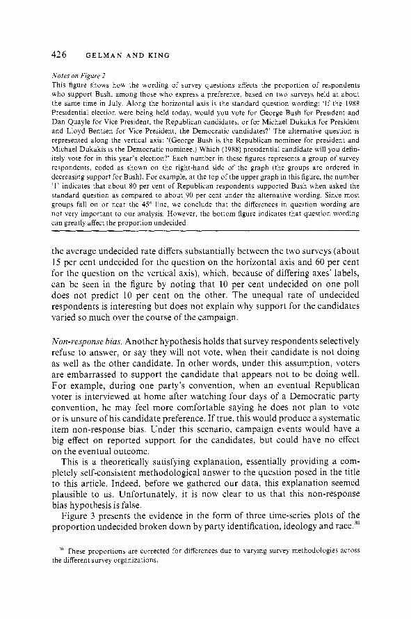
This is a theoretically satisfying explanation, essentially providing a completely self-consistent methodological answer to the question posed in the title to this article. Indeed, before we gathered our data, this explanation seemed plausible to us. Unfortunately, it is now clear to us that this non-response bias hypothesis is false.

Figure 3 presents the evidence in the form of three time-series plots of the proportion undecided broken down by party identification, ideology and race."

'' These proportions are corrected for differences due to varying survey methodologies across the different survey organizations.


Undecided rate by party ID Undecided rate by ideology 0.6 r 1 0.6,

0.0 I 0 . 0 L -200 -150 -100 -50 0 -200 -150 -100 -50 0


0.5 - 2 0.4 - 2

0,3 rn 5 0.2 -

0.1 -


Undecided rate by race 0.6 1

. \ .' \

- - - I*' *\,.:-y' 'nd, * - , - - - ? \.-**

,,.. ... ...... 8 ....... .--... Rep ..,..... ".... .. . ..... ., 9 .$., i Dem .,:'.,

0.0 -200 -150 -100 -50 0


...I.

I ,... ;.- 2 0.4 mod ,----- - _ .& - .?- 2 - 1 ons' ,,'--.-- .................... . 3, .

z a~l!ib- , '. . . rn I 5 0.2

0.1

Fig. 3. Trends in undecided respondents, 1988

Notes: This figure includes three time-series plots of the proportion of survey respondents who report being undecided as to their vote. Each line in a plot represents a different group of voters. The party identification graph tracks political independents ('Ind'), Republicans ('Rep'), and Democrats ('Dem'). The ideology graph tracks ideological moderates ('mod'), conservatives ('cons'), and liberals ('lib'). The final graph plots white and non-white respondents. In most cases, the lines representing different groups within each figure move in the same rather than opposite directions, which confirms that the proportion undecided did not vary by these groups.

As can be plainly seen, the proportion undecided does not vary dramatically over the course of the campaign. But, more important for this hypothesis is that the groups vary together, whereas if the non-response bias hypothesis were true we would expect the opposite. Thus, it could not be that Republicans are more likely to report being undecided during the Democratic convention, and conversely. The same holds for race and for ideology.3'

'' Other variables also give similar results. We show in the Appendix that party identification and ideology are largely exogenous variables, not responding much to changes in voter preferences or anything else that changes during the campaign.

3.2. Journalists' Theories

An alternative way to resolve the paradox of volatile polls and accurate forecasts is to dismiss the forecasts, as in the first hypothesis below, or to accommodate the forecasts to the journalists' interpretation of the polls, as in the second hypothesis.

The forecasters were lucky because Bush ran a good campaign and Dukakis a poor one. The simplest way to dismiss the pre-campaign forecasts of the political scientists and economists is to say they were just lucky and happened to coincide with Bush running a good campaign and Dukakis running poorly. Evidence for this hypothesis is that Bush's rapid gain in the polls coincided with what seemed to be his particularly adept campaigning.

The success of out-of-sample forecasts discussed in Section 1 causes us to doubt this hypothesis. Moreover, as discussed by ~ e w i s - ~ e c k , ~ * several other scholars have also produced relatively successful presidential election forecasts (for previous elections) based on different statistical models.33 All these models do reasonably well in many election years, not only 1988. The success of all these forecasts is clearly due to more than chance, and we feel that, at this point, the burden of proof lies with the critics who still believe the forecasters are merely lucky.

In addition, what seemed to the journalists to be Bush's adept campaigning might just be a justification in hindsight of what 'explained' the polls. How can we test this alternative explanation of the media's interpretation? In other words, what can be done to avoid rationalization after the fact? One possibility is to use what journalists identified as the keys to success in previous campaigns and see how the Bush and Dukakis campaigns should be judged according to those rules.

This is easily resolved: in all recent presidential election campaigns before 1988, the main rule, according to the media, was which candidate was better at 'acting presidential'. Bush was the first candidate in modern times directly to attack his opponent, which clearly violates the rule. In recent previous campaigns, this task was taken up by the vice-presidential candidate, campaign commercials, or prominent supporters, but never by the presidential candidate.

Thus, from this media perspective, Dukakis actually looked better than Bush during the campaign, since he was acting in more presidential style. If the polls had continued to favour Dukakis, and he had won the election, we doubt whether the media would have changed their criteria for evaluation. It may be that Bush's strategy was effective, but in this case the 1988 election provides only a hypothesis, not a confirmation of one. On the other hand, although resolving these points without careful studies of the effect of campaign media events is probably impossible, it does seem (almost!) undeniable at other times that events in the campaign do influence the poll results.

3' Lewis-Beck, 'Election Forecasts in 1984: How Accurate Were They?' 3 3 See, for example, Fair, 'The Effect of Economic Events on Votes for President' and updates.


Unbalanced campaigns or predictable convergence. Another hypothesis holds that the polls were accurate indicators of the candidates' fortunes throughout, and that they varied because Dukakis was legitimately ahead at the start of the campaign while Bush ran a better campaign and won the election. Rather than claim that the forecasters were lucky, this model assumes that the election result was successfully forecast because the convergence of the poll results to the general election outcome was predictable. Thus, under this hypothesis, support for the candidates really did change over the campaign, but this change was successfully predicted by the forecasts.

This hypothesis mixes journalists' and political science theories, in that it accepts the forecast, but still follows the story of the polls to understand why Bush won. It accords with the methods, but not the theories, of political science.

This hypothesis has a reasonable construction and is internally consistent. However, it does not explain why any forecasts should predict that Bush would run a better campaign - especially since the forecasting models include nothing which measures the two candidates' skills as campaigners. Certainly few journalists had any idea this was going to happen. Moreover, if Dukakis's advisers could have predicted that they were going to run a poor campaign, they certainly would have changed their strategy - thus making the forecast incorrect.

Uninformed voters. A final explanation posed by journalists is at the level of the voter. According to this idea, many people, or at least enough to swing elections, vote on the basis of factors that political scientists would not call 'fundamental', such as the personality of the candidates, gaffes, speaking style, campaign events and the like. Under this explanation, the voters who decide this way may truly care about these factors, or may just not know enough about the fundamental variables to make an informed decision. This model explains the swings in the pre-election polls, but does not explain how pre- campaign forecasting methods predict so well, given that the political science forecasts do not even try to account for personalities and campaign events.

3.3 Political Science Theories

In contrast, the political science theories take as a starting point that the ability of economists and political scientists to forecast election results accurately months ahead of time is evidence that the election came out just as predicted. We present two flawed explanations here: the first is quite possibly true, but incomplete, as it does not address the relation between the campaign and the opinion polls. The second hypothesis is plausible but can be refuted by our individual-level poll data.

Balanced campaigns. Under this hypothesis, forecasting models worked in 1988 because the campaigns were balanced, and thus the election outcome occurred roughly as Rosenstone and others had predicted on the basis of information available months before the election.

Although most journalists seem to deny it, political scientists believe this hypothesis to be almost certainly true. Unfortunately, even if true, it provides

no solution to the key puzzle in the context of a model of voter decision making. The 1988 presidential election, like all modern presidential elections in which no incumbent was running, pitted two major-party campaigns that were roughly equal in strength and resources. There are plenty of examples during the campaign when astute political observers could suggest instances where one candidate could have done something better, but with equal funding and the best advisers each party has to offer, it would be surprising to see a campaign as unbalanced as for many voter referendums or for numerous local elections. We suspect that if a presidential election happened to be severely unbalanced (beyond the predictable unbalance associated with incumbency), political science forecasting models would probably not perform well. We happen not to have observed any such instances in modern times.

The fact that modern presidential campaigns seem to be balanced, which is consistent with the political science model of voter decision making, does not solve the puzzle about why the polls varied so much. The media wisdom about the 1988 election is that the outcome is explained by Dukakis running a poor campaign. Of course, this denies the hypothesis that the campaigns are balanced.

Thus, under the political science model, balanced campaigns cause no theoretical problems, but they say nothing about why the polls should vary so much. Under the journalists' model, balanced campaigns are inconsistent with the observation that the polls vary a lot. In neither case does this hypothesis explain the paradox.34

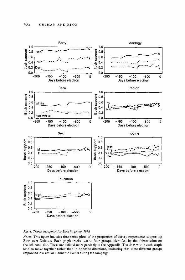
Partisans returning to the fold. Under another hypothesis, in January there is a large mass of undecided voters, and over the course of the campaign, the number of those who report being undecided drop, as different groups move towards their natural home. This is observationally similar to the non- response bias hypothesis, but is theoretically very different. An elaboration of this hypothesis is that strong partisans come home to their party first, then weaker partisans, and so on. Different events bring in different groups of voters, but under the hypothesis being discussed here, the strong ones come home first, then subsequent events bring in others later. In this model, the campaign ratchets in new groups of voters, who, once they migrate to the 'decided' category, tend to stay with their preference - perhaps due to psychological justification mechanisms.

The key evidence against this thesis is that the proportion of undecided voters does not drop over the course of the campaign (refer back to Figure 3). It is especially noteworthy that the proportion undecided does not drop during times of massive shifts in the polls (as recorded in Figure 1). The elaboration of this hypothesis also seems wrong since strong Republicans supported

34 The two models are also inconsistent with one another about the evidence they provide on who ran a better campaign in 1988. Contrary to the journalists' claims (and even Dukakis himself), most political science models showed Dukakis doing as well or even better than expected, perhaps because Dukakis's vice-presidential selection was better (from an electoral perspective) than Bush's.


Bush from the start, and did not move much over the course of the campaign. This can be seen in the first time-series plot of Figure 4 of Bush support by party ident i f i~at ion.~~ Moreover, support for Bush among the Democrats actually increased during the campaign, exactly opposite to what would be expected under this hypothesis. Short-term changes in overall support for Bush (conceivably in response to specific campaign events) actually appear to occur for Democrats, Republicans and Independents equally: the three series move together. Indeed, the same appears true for Bush support broken down by the other variables in Figure 4. It thus appears quite clear that support for this hypothesis in these data is largely non-existent.

We do believe that voters are coming home to their natural preferences, but not that they are following the particular pattern of returning to the fold by party identification.

3.4. Rational Actor Theories

These theories are also political science theories, but they differ from those in the other categories because they are based on specific assumptions about individual voters. Because of the lack of any contrary evidence, we assume for each of the theories that voters answer survey questions about candidate support sincerely. This is consistent with theoretical evidence from two- candidate, winner-take-all races, where there is not much point in strategic voting. Moreover, it does not differ dramatically from the voting situation which, although somewhat more behavioural, is not more costly.

Full information. Consider first the extreme version of the rational actor model. According to this model, people

(1) have full information throughout the campaign about their fundamental variables,

(2) are using all the information they have at any time to form their survey response or voting decision, and

(3) are rationally accounting for this uncertainty, in the sense of maximizing some expected utility.

If this model were accurate, political scientists would still forecast accurately, but the trial heat polls would not change at all over the campaign. Since the polls obviously do change, this model can be rejected, but it will nevertheless be useful in clarifying related models, as well as our preferred explanation presented in Section 4.

Incomplete information. An incomplete information model assumes, from the full information model, that (1) is incorrect, but (2) and (3) hold. That is, voters gather information over the campaign, use this information in making their decisions, and rationally account for their uncertainty. If this model,

'' The Appendix shows that party identification and ideology in the population are roughly constant during the campaign.

Ideology

Days before election Days before election

Race Reaion


Sex Income 1.0 1 < 1.0.

0.0 I 0.0 - -200 -150 -100 -500 0 -200 -150 -100 -500 0


Education

0.0 I -200 -150 -100 -500 0


Fig. 4. Trends in supportfor Bush by group, 1988

Notes: This figure includes time-series plots of the proportion of survey respondents supporting Bush over Dukakis. Each graph tracks two to four groups, identified by the abbreviation on the left-hand side. These are defined more precisely in the Appendix. The lines within each graph tend to move together rather than in opposite directions, indicating that these different groups responded in a similar manner to events during the campaign.


were correct, political science forecasts would work, as they do. On average over the whole campaign, we would expect changes in polls to occur in the direction of the forecasts; that is, as voters gathered more information, they would gradually move in the direction of their fundamental variables. This, too, is consistent with the evidence.

However, the model implies that changes at any one time during the campaign would be relatively small, because voters would appropriately judge their uncertainty, at all times estimating the values of their fundamental variables and candidate positions. Sharp short-term changes in the polls - deviations from a trend towards the forecast poll positions - would occur only when campaign events were unexpected, such as if a candidate did much better than expected in a debate, or made a surprise change in his or her stand on an important issue.

This model is partly right, but since we find (and show below) that the polls do respond to information that almost certainly was anticipated by voters, we reject this e ~ p l a n a t i o n . ~ ~

4. T O W A R D S A N E X P L A N A T I O N F O R P O L L V A R I A T I O N

Section 3 raised and then provided sufficient evidence to dismiss several plausible hypotheses of why the trial heat polls vary so much, even given our ability to forecast presidential election outcomes. We now turn to our preferred, but quite tentative, explanation, for which we present evidence in Section 5.

Our working hypothesis is that voters cast their ballots in general election contests for president on the basis of their 'enlightened preferences'. As with the concept of enlightened preferences in the political philosophy ~iterature,~' we do not require that people be able to discuss these preferences intelligently or even to know what they are; we only require that they know enough that their decisions are based on the true values of the fundamental variables. The function of the campaign, then, is to inform voters about the fundamental

'6 According to Condorcet's 'jury theorem', if some voters have incomplete information, then, under certain conditions. a majority-rule electoral system will produce outcomes equivalent to the situation that would exist if all voters were informed. This is obviously relevant to our inquiry, except that the assumptions required to prove this theorem are far too restrictive. Scholars have recently been quite successful at dropping some of these restrictive assumptions, so perhaps in the near future the two lines of research might converge. (See Nicholas R. Miller, 'Information, Electorates, and Democracy: Some Extensions and Interpretations of the Condorcet Jury Theorem', in Bernard Grofman and Guillermo Owen, eds, Information Pooling and Group Decision Making (Greenwich, Conn.: Jai Press, 1986); Krishna Ladha, 'Condorcet's Jury Theorem, Free Speech and Correlated Votes', American Journal of Political Science, forthcoming.) Related work in experimental economics has studied how markets proceed on the road to various types of equilibria. (See Charles R. Plott, 'An Updated Review of Industrial Organization: Applications of Experimen- tal Methods', in R. Schmalensee and R. D. Willig, eds, Handbook of Industrial Organization, Volume 11 (Amsterdam: Elsevier Science Publishers, 1989); and 'Industrial Organization Theory and Experimental Economics', Journal of Economic Literature, 20 (1982), 1485-1527.)

'' Dahl, Democracy and Its Critics.


variables and their appropriate weights; notably, the candidates' ideologies and their positions on major issues.

According to this explanation, only the second of the three assumptions under the full information rational actor model (see Section 3.4) is correct. That is, voters do not have full information and do not rationally judge or incorporate their uncertainty, but they do gather and use increasing amounts of information over the course of the campaign, with the largest increase occurring just before election day.38 We also assume that voters answer surveys about candidate support sincerely. We elaborate this model here.

At the start of the campaign, voters do not have the information necessary to make enlightened voting decisions. Gathering this information is costly and most citizens have no particularly good reason to gather it in time for the pollster's visit, so long as it can be gathered when needed on election day.

Most polls ask whether the respondent intends to vote, and the question appears to be answered sincerely and relatively accurately. Likely voters with insufficient information at the time of the poll still report that they will cast a ballot on election day. Unfortunately, those who consider themselves 'voters' are willing to report to pollsters their 'likely' voting decisions, even if they have not gathered sufficient information to make this report accurate. The reason is the quite general point, as much psychological research has shown, that human beings are very poor at estimating uncertainty and at making fully rational decisions based on uncertain or incomplete i n f ~ r m a t i o n . ~ ~ People also make decisions based on these incorrect uncertainty judgements, producing, in only this narrow sense, 'irrational' decisions. Compounding the problem is the awkward situation of the survey interview: imagine survey respondents, who, when asked, indicate that they will vote; then they, when later asked for the name of the candidate who will get their vote, are embarrassed to reveal their ignorance or uncertainty, especially after already saying that they would vote.40

Thus, without sufficient knowledge of their fundamental variables, and when asked to give an opinion anyway, most respondents act as they will in the voting booth on election day: they use information at their disposal about their fundamental variables, and report a 'likely' vote to the pollster. We believe that this report to the pollster is sincere, but the survey response is still based

'' See Samuel Popkin, The Reasoning Voter: Communication and Persuasion in Presidential Cam- paigns (Chicago: University of Chicago Press, 1991).

" Daniel Kahneman, Paul Slovic and Amos Tversky, eds, Judgment Under Uncertainty: Heuris- tics and Biases (New York: Cambridge University Press. 1982).

Designing surveys so as to reduce this embarrassment, making it easy to report 'no opinion', would not necessarily improve the forecasting ability of the polls, since those voters who express a 'certain' opinion seem to mirror the survey population as a whole; see the discussion of question wording in Section 3.1 and Figure 2. A very useful future research project would be to design a survey or experiment to encourage voters to account rationally for their uncertainty (perhaps by giving them more time or financial incentives to give the 'right' answer), and see if it makes a difference to their reply.


on a different information set from that which will be available by the time of the election. It will therefore differ systematically from the eventual vote to the extent that the voter's information set improves over the course of the campaign. In relatively high-information, balanced campaigns, voters gradually improve their knowledge of their fundamental variables and generally have sufficient information by election day.

Thus, the campaign itself will confer no large unexpected advantages on one party or the other. This accounts for forecasting models, based on information available only at the start of the general election campaign, working well. However, this does not make the campaign irrelevant, because without it election outcomes would be very different. Moreover, if one candidate were to slack off and not campaign as hard as usual, the campaigns would not be balanced and the election result would also be likely to change. Thus, under this explanation, presidential election campaigns play a central role in making it possible for voters to become informed so they can make decisions according to the equivalent of enlightened preferences when they get to the voting booth. This process then depends on the media to provide information, which they do throughout the campaign, and the voters to pay attention, which they do disproportionately just before election day.

Note that we are not arguing that there exists an identifiable group of uninformed voters, who gradually become more informed than other groups over the course of the campaign. While it is undeniably true that knowledge varies considerably across citizens at any one time, we find that virtually all groups of eventual voters have their preferences gradually enlightened during the campaign by roughly the same amounts.

If this explanation of our central puzzle is correct, the only remaining question is not why the polls move in the direction they do; we already know that they move in the direction of the political scientists' forecasts. The relevant question is why they begin where they do. Our hypothesis is that the early position of the polls is a result of the information that is readily available at the start of the general election campaign. For example, Dukakis's race against Jesse Jackson alone at the end of the Democratic nomination positioned him as quite conservative. In part as a result of this, Dukakis was seen at the start of the general election campaign as more conservative than he was (and at times even more conservative than Bush). As citizens learned more about the appropriate values of their fundamental variables, voter support for the candidates responded.

5 . E V I D E N C E FOR E N L I G H T E N E D P R E F E R E N C E S

As we indicated at the start of this article, we have much more evidence about why many possible explanations are wrong than about which one is right. In particular, we are handicapped in our analysis here by having no direct measures of voter information over the campaign, or of some of the fundamental

variables the forecasters use in their model^.^' Our strategy, then, is to extract whatever information is available in our data, and leave it to future research to more firmly establish or refute this explanation.

We begin by providing evidence that preferences early in the campaign are relatively unenlightened. From one perspective, this should neither be difficult nor perhaps even necessary to show, since numerous scholarly studies have demonstrated the ignorance of Americans about most matters of policy and politics. However, we do not require citizens to be able to verbalize their motiva- tions or detailed positions on their fundamental variables. The idea of making voting decisions on the basis of enlightened preferences only requires that voters cast their ballots in the same manner as they would if they had full information and time for a complete consideration of all issues. Thus, survey questions about citizen knowledge would not directly answer our concerns. For the same reasons, it would also not be a good strategy to ask survey respondents what their fundamental variables are. A measure of the 'revealed preferences' of this group of citizens would be better, but one cannot observe individual-level political behaviour in polling data.

Instead we look for systematic discrepancies between actual voter support and expected support, which we calculate on the basis of measured demographic and fundamental variables. We do this in four different ways in this section, each a different observable consequence of the same theory of poll variation described in Section 4. We begin in Section 5.1 by demonstrating the 'irrationality' of early poll movements. Section 5.2 shows that the fundamental variables are of increasing importance over the campaign. We explore how voters weight the fundamental variables in decision-making in Section 5.3 and demonstrate in Section 5.4 that changes in these weights, and not the values of the variables, are what account for polls fluctuations.

5.1. The 'Irrationality 'o f Early Poll Movements

We first demonstrate that voters do not 'rationally' account for uncertainty in using information to make decisions about supporting presidential candidates. We show this by focusing on predictable changes associated with totally expected campaign events, something that should not occur if survey respondents were fully rational.

Figure 1 presents the proportion of supporters for each party over the course of the campaign, and marks the dates of the Democratic and Republican party conventions. In order to see the effects more clearly of these party conventions on support for the presidential candidates, Figure 5 plots the proportion sup-

" Some of the most important variables forecasters use do not change over the course of the campaign, such as incumbency status and some other national variables. That we have no information on these does not affect our inferences because they are effectively controlled by being held constant. The remaining variables that might have some effect include perceived economic well-being and perceived ideological distances between voters and candidates, both of which might change over the campaign.


porting the Republican candidate before and after each convention since 1964.~' Republican conventions are marked 'R' and Democratic conventions marked 'd'. If a point appears above the 45" line, Republican support went up after the convention; if it is below the line, Republican support dropped. If these conventions had no effect on the level of support, the points would be scattered randomly on and about the 45" line. The results are unambiguous: support for the Republican candidate increased after all Republican conventions and decreased after all but one Democratic convention. The 1988 conventions, which are circled, are fairly typical of the points on the graph, lending credence to our more detailed analysis of that election year.43

0.3 0.4 0.5 0.6 Republican support

before the convention

Fig. 5. Effects ofparty conventions on presidential campaign polls, 196448

Notes: This figure summarizes all the plots in Figure 1 before and after the party conventions. Each 'R' refers to survey support for the Republicans before and after a Republican convention; each 'd' indicates support before and after a Democratic convention. When a symbol appears above the 45" line, it indicates that support for the Republican candidate increased during the convention, whereas symbols below the line indicate that support for Bush declined. Note that all R's appear above the line and almost all d's appear below the line. The 1988 conventions are circled and appear typical of public opinion swings during the conventions.

42 We omit 1952-60 from Figure 5 because Gallup did not list polls between the two conventions for those years.

James E. Campbell, Lynna L. Cherry and Kenneth A. Wink, 'The Convention Bump', Ameri- can Politics Quarterly (1993, forthcoming) also discuss poll movements during conventions.

The clear results from Figure 5 are consistent with our explanation in Section 4, for if people were informed and reflective about their candidate preferences early on in the campaign, they would also be able to predict that their opinions will change after each party convention. In that case, they would realize that they should change these preferences immediately. Thus, if people were rationally incorporating their uncertainty about future events we would not witness any predictable changes in support for the candidates. Recall that if the full or incomplete information rational models were correct, only unexpected information would change voter preferences. Yet, almost all aspects of modern political conventions have also been extremely predictable, from the nominee to most aspects of the platform, and even the 'spontaneous demonstrations' on the convention floor for various candidates. We know the conventions produce almost exclusively expected information from merely watching the news on the days leading up to the conventions. Moreover, any voter who was aware during the convention four years earlier (or was reminded of this by the media) should not be surprised by anything that happens during any recent political c ~ n v e n t i o n . ~ ~

This logic also applies more generally, if the political science forecasts can be believed. Since we can predict which candidate respondents will end up supporting on election day, if they were enlightened at the start, or rationally incorporated their uncertainty all along, they would change their preferences only minimally throughout the campaign. Since they do change their preferences, and since convention changes and other changes are largely predictable, we conclude that many people are unenlightened at the beginning of the campaign and are not rationally incorporating uncertain information in their decisions.

Another observable implication of the enlightenment hypothesis that we can evaluate is whether these changes are also predictable for subgroups of the electorate. Our data on groups include all two-way interactions among ideology, region, education, sex, income, party and race - all the covariates on which we had information for a large number of our sample surveys (see the Appendix). Two-way interactions include all combinations of groups such as non-white Democrats, highly educated Southerners, lower-middle income males, conservative females, e t ~ . ~ ~

Figure 6 contains a particularly compact way of presenting a large subset of this group-level information. Consider first the party graph in the top left

" A small amount of uncertainty is reduced by the conventions, but this could not account for the systematically predictable shifts in voter support in Figures 1 and 5.

45 We also tried the following analyses with all three-way interactions and obtained similar results, except that the many groups with small numbers of voters increased sampling error and thus made the results much more variable and more difficult to interpret.


6A: Democrats, Independents and Republicans 6D: Non-whites and whites

0.2 0.4 0.6 0.8 Final Bush support

60: Democrats, lndependents and Republicans


6E: Non-whltes and whites

0.2 0.4 0.6 0.8 0.2 0.4 0.6 0.8 Final Bush support Final Bush support

6C: Democrats, Independents and Republicans 6F: Non-whites and whites

I I



Fig. 6. Changes in support for Bush by subgroup, 1988

Notes: This figure shows opinion changes for different groups of respondents during key periods in the campaign. Each of the three plots on the left (labelled 6A, 6B and 6C) shows different subgroups classified by party identification; circles show subgroups of Democrats (such as liberal Democrats, white Democrats, rich Democrats, poor Democrats, etc.), triangles show Independent subgroups, and squares show Republican subgroups. The plots on the right (labelled 6C, 6D and 6E) are divided into subgroups of non-whites (shown by diamonds) and whites (triangles). The size of each symbol (as measured by the area of a circle that could be drawn around it) is proportional to the number of survey respondents in the subgroup. In each plot, the horizontal axis indicates, for each displayed subgroup, the proportion of respondents who supported Bush in the polls in the last days before the election, and the vertical axis indicates the change in support for Bush in the period shown by the plot, from before to after the Democratic convention for 6A, the Republican convention for 6B, and the last forty days of the campaign for 6C.

(labeled 6A) of the figure. Each of the two-way groups that include party classification is plotted on this graph, with eventual Bush support on the horizontal axis and the trend in Bush support on the vertical axis. For the three graphs in the first column, this trend in Bush support is calculated as the change from before to after the Democratic convention (for 6A), the Republican convention (for 6B) and the last forty days of the campaign (for 6C), respectively. We define only the party of each group by the type of symbol drawn -circles for Democrats, triangles for Independents and squares for Republicans. The size of each symbol (as measured by the area of a circle drawn around it) plotted for each group is proportional to the number of respondents it includes. Figure 6A shows that all Republican groups eventually support Bush very strongly (all the squares are to the right on this graph), with only one small group (the non-white Republicans) containing fewer than 80 per cent Bush supporters. All democratic groups also end up being Dukakis supporters, although their support has a lower mean and higher variance. Independent groups end up nearer to the middle, although most do wind up giving Bush majority support.

Figure 6A also demonstrates that almost all of the many groups during the Democratic convention predictably increased their support for Dukakis (as shown in Figure 6A by almost all the symbols being below the horizontal line drawn at zero change). Independents moved the most in this direction, but change among Democrats and Republicans is about the same. Figure 6B shows the same relationship for the Republican convention; and the results are a mirror image, with almost all groups increasing their support for the Republican party's nominee. Democrats appeared to change somewhat more than Republicans, and Independents still changed the most, but the pattern is about the same.

Figure 6C portrays the trend in support for the candidates over the last forty days of the campaign. In this period, the action was among the Democratic and Independent groups, most of which steadily moved towards Bush. Most Republican groups changed very little from their already high level of Bush support.

In total, the three party graphs (Figures 6A, 6B and 6C) provide additional, more detailed group-level evidence. They show that even among the many groups of voters studied here, party conventions do not consolidate support among one's own partisans, but rather affect partisans of both types in similar and predictable ways. These graphs also show that Independents, and in general groups near the middle, respond most extremely to the conventions. This is consistent with our hypothesis, but not because these citizens are the least enlightened. Instead it is because these voters tend to be on the margin; thus, changes in knowledge of fundamental variables produced by the conventions produce larger shifts in the fraction of respondents supporting one candidate or the other than other groups not so near the margin. The same is true of other party groups which are near the middle of the graphs. Thus, this evidence is consistent with the idea that all voter groups become enlightened by roughly


the same amount over the course of the campaign, even though this has different effects on voter support for the various groups.46

Finally, Figures 6A, 6B and 6C demonstrate that the picture was somewhat asymmetric with respect to the parties during the period after the last convention, and even partially during the Republican convention. Since Republican groups supported Bush much more uniformly than Democrats supported Duk- akis (as is evidenced in the figures by the relative dispersion of the squares as compared to the circles), this too is consistent with the idea that voter groups more divided in support will respond more to changes in fundamental variables. But this result can also be explained in a more direct, substantive way: Bush supporters were more unified in part because Bush was the candidate more known by the public. Dukakis was a more unknown quantity; it should be no surprise that early voter support among Democrats were more spread out between the parties. And because more of these voters were closer to indifference between the two candidates, changes in knowledge of their fundamental variables will have more of an effect.47 Thus, roughly the same change in enlightenment that occurs to all citizens has different effects depending on their earlier support for the candidates.

Figure 6 also contains analogous figures for racial groups (labelled 6D, 6E and 6F, with non-whites represented by solid diamonds and whites by open triangles), and the conclusions are largely the same. The Democratic party convention increases support for Dukakis, and the Republican convention increases support for Bush, among almost all groups of white and non-white voters. Exceptions in these graphs include a group of white liberals and white Democrats, each of which appears to act more like the non-white groups. There is also a small group of non-white Republicans which appears among the white groups. During the three periods, the white groups are somewhat more cohesive and less variable.

5.2. The Fundamental Variables' Increasing Importance During the Campaign

If voters are becoming enlightened, then the fundamental variables should be increasing in importance over the campaign. Figure 6 is consistent with this hypothesis since individual groups are becoming more homogeneous, thus increasing heterogeneity across groups, even within parties. More generally, if

4h We have conducted extensive analyses, not presented here, searching for identifiable groups of respondents who become relatively more 'informed' or 'enlightened' as the campaign progresses. Even using education and many other variables, we have found no clear evidence for differences across groups in the speed with which they learn during the campaign.

47 Indeed, this concept should be useful for predicting changes in group support over the campaign. In general, groups that are more divided at the start of the campaign will move the most as the campaign progresses.


voters are basing their survey responses more on the fundamental variables over the course of the campaign, as we hypothesize, then groups of voters (categorized by these variables) should become increasingly distinctive - homogeneous within and heterogeneous across the groups. The observable implication of this process which we now evaluate is the extent to which voter groups are more heterogeneous as the campaign progresses.

7C: Estimated heterogeneity among Independent groups

2 0.10

7A: Estimated heterogeneity among Republican groups 78: Estimated heterogeneity among Democratic groups

-150 -100 -50 0 Days before election

5 0.12- Q P 2 0.10-

" 0.08- z 2 .- E m 0.06- .- -$'0.04- E m 0.02 z $ 0.0-

Fig. 7 . Heterogeneity among subgroups, 1988

Notes: Each circle in Figure 7A corresponds to a different national survey, with a measure of heterogeneity among subgroups of Republicans plotted vs. the date of the survey. The heterogeneity measure is an estimate of the standard deviation in support for Bush across the subgroups, corrected for the sampling variability in the poll. The dotted line is a smooth curve designed to show the trend over time. Figures 7B and 7C similarly show heterogeneity across subgroups of Democrats and Independents, respectively. The increase in heterogeneity for two of these graphs indicates that survey respondents are sorting themselves out more clearly into their respective subgroups.

-150 -100 -50 0 -150 -100 -50 0 Days before election Days before election

0 0 O o D 0 o

, e ............... -.......: ............... pb ...... : ..... 0 0 ..:.... An- o "

m 0 0 0 m o 00 ,

One confirmation of increasing homogeneity within individual groups, and consequently increasing heterogeneity across groups, is shown in Figure 7. This figure plots a measure of the true heterogeneity across subgroups within

5 0.12) Q Q 2 0.10-

" 0.08- .- z 2 .- E m 0.06' > b $- 0.04-

n 0.02. - 6 0.0-

0 '=e o ,a ,Pi

0 0 ,., 0 .... o 0 ........... i...: .A' ................. B. ..?..-....... a 0

0 0

0 0 0 0 0


parties by measuring the observed variance in support for Bush across subgroups and subtracting the expected sampling variance of this measure.48

We consider each party separately in Figure 7 so as to see fine detail; if groups in different parties were included, the variances would be so large as to dwarf the changes over time.

Each circle in Figure 7 plots our measure of the heterogeneity across groups for a specific time during the general election campaign. For help in viewing trends in this graph, we plot a non-parametric regression line on each (called ' l o ~ e s s ' ) . ~ ~ Consistent with the idea that enlightenment occurs throughout the campaign, heterogeneity across groups is clearly increasing for the Democ- rats and Independents throughout the entire campaign (i.e., partisans are sorting themselves out more clearly by subgroup). As would be expected, this enlightenment occurs mostly just before election day, when voters must pay attention if they are to vote on the basis of their fundamental variables. However, heterogeneity is not changing noticeably among Republican groups. This is consistent with the idea that enlightenment, occurring to all citizens at roughly the same degree and speed, has the largest effect on the voter preference of groups, such as Independents and those who are the eventual supporters of the more unknown candidate, which were more indifferent between the candidates. Although we had guessed that the line for the Republican graph would be increasing too, it should be no surprise that many fewer Republicans were indifferent early on between a Republican incumbent president and a considerably less well-known Democratic challenger.

5.3. How Respondents Weight Fundamental Variables

We can now more directly address the issue of the role of the fundamental variables and the weights given to them by survey respondents throughout the election campaign. We do this by using all available covariates to predict support for Bush or Dukakis with a logistic regression in each survey. These explanatory variables - party, ideology, race, sex, income, education and region - are not perfect measures for what political science research has taught are the fundamental variables on which most citizens base their voter preferences, but they are the best we have available given what questions happened to

48 For each of the three 'parties' (Democratic, Republican and Independent) and each poll, let x , , xz, x, , x, . . . be the average support for Bush in all the subgroups of that party (for example white Democrats, non-white Democrats, liberal Democrats, moderate Democrats, etc.), and let n , , n2 , n,, no . . . be the survey weights of the respondents in each subgroup of the party. The mean support for Bush in the party is 2 = Zin,xiEin, , the observed variance across subgroups is: Zin , ( x i - $/Z,n,, and the expected sampling variance is: Z,n,x,( l - x,)iZ,n,. Each circle on Figure 7 plots the difference between the observed variance and the expected sampling variance, set to zero if the difference is negative.

49 Each point on the 'lowess' curve is calculated by weighted least squares, with the points in closest proximity on the horizontal axis given the highest weights. See William Cleveland, 'Robust Locally Weighted Regression and Smoothing Scatterplots', Journal of the American Statis- tical Association, 74 (1979), 829-36.


be asked in the surveys. They are also the most important individual-level variables, since scholars have found that incumbency and economic variables in the United States affect the vote decision primarily through their true, and not perceived, values.

Certainly party, ideology and race are among the fundamental variables, and all are expected to have a strong effect on voting (or support) decisions. Sex should have a small effect, with women supporting the Democrats slightly more; income and region should have a somewhat larger effect; but, conditional on the other variables, education should have almost no effect. The fact that we do not have measures in these surveys of all the variables the forecasters use in their models is a real limitation of this logistic regression analysis, and this is an important area where future research should focus.50 These hypotheses from previous research only suggest the weights of the fundamental variables in the final analysis, as election day nears. Our enlightenment hypothesis suggests that early on in the campaign the importance of these variables may be different, although exactly what that difference is, we do not predict.

Figure 8 presents a summary of the results of our logistic regression estimates. Each graph in this figure plots the effect of a variable over time, with each circle representing the analysis of a single survey (except in the two weeks before the election, when some groups of surveys taken on the same day were analysed together). Each circle on each graph is the difference between the probabilities of supporting Bush for two voters who are identical in all ways, except for the variable in question. Using these 'first differences', instead of the original logit coefficient, enables us to interpret the results of the scales of the original variables;" the Appendix defines the variables and the size of the shifts used to calculate the first differences. In addition, we add a least- squares straight line fit to these points in order to highlight patterns.52

The party graph at the top left of Figure 8 indicates that, holding all the other variables constant (at their midpoints), Republican identifiers support Bush about 70 percentage points more than Democratic identifiers, a strong effect that does not change appreciably over the course of the campaign. The right side of each graph shows the effect of the corresponding variable near election day. In all cases, this is roughly as one would. expect from reading the political science literature. The exact numbers would not be precisely predicted, but the figures here are no surprise. Conservatives support Bush at the end of the campaign about 40 points more frequently than liberals. Whites support him about 30 points more than blacks. Northern whites support him

In fact, we do have many additional survey questions aside from those we analyse, but these were not asked in as many polls. Thus far, our auxiliary studies of these questions do not suggest any changes in the conclusions presented in this article.

" See Gary King, Unifying Political Methodology: The Likelihood Theory of Statistical Inference (New York: Cambridge University Press, 1989). '* Because we used only surveys which had all of our covariates, there are fewer points in

this figure. With this smaller sample size, the 'lowess' estimates used in Figure 7 were less useful here.


.c Party Ideology

' 0.6

0.3

m P ; 0.2 S 0.2 C

0 0.1 $ 0.0 2 0.0 .............................................................................

-1 50 -100 -50 -150 -100 -50 0 Days before election Days before elect~on

Region (among whites)

g 0.10

5 0.05

$ 0.0 ............................................................................. -150 -100 -50 0 -1 50 -100 -50 0


Region (among nonwhites) r Sex .c

0 0.05

LO c

; -0.10

f -150 -1 00 -50 0 -150 -1 00 -50 0


.c Income Education

0,06 a o,02v] - ......... "".. .......................................................... r o,o " "

P 4 0.02

0

m 0 9-0.02 m 0 C ............................................................................. + S - $ -0.02 0 w $ -0.06

-150 -100 -50 0 -150 -1 00 -50 0 Days before election Days before election

Fig. 8. Estimatesfrom logistic regressions, 1988

Notes: This figure summarizes the results of logistic regression estimates of vote intention. Each plot in this figure portrays the effect of a variable over time; the variables are listed in order of decreasing effect size. (Note that the vertical axes of the plots are not on a common scale.) Each point on each plot is the difference between the probabilities of supporting Bush for two voters that are identical in all ways except for the variable in question. Each plot has a horizontal dotted line at zero. In addition, a linear regression fit is shown, as a solid line, in each plot to highlight the time trends.

446 G E L M A N A N D KING

about 15 points more than southern whites, whereas there exists no regional difference at the end of the campaign among non-whites. Income and sex have moderate effects in the expected direction, and education has essentially no explanatory power at all.

The graphs also show the weights of these fundamental variables over the entire campaign. For most of these variables, the effect estimates vary considerably. Race and ideology matter less at the start of the campaign than at the end, whereas the effect of region among non-whites and the effect of gender are much higher early on.

Political science research and our thesis explain fairly clearly why the right sides of these graphs should look as they do. That the early effect estimates (on the left sides of the graphs) differ from these eventual results is also consistent with the idea of voters becoming enlightened over the campaign. What, then, would be the explanation for the particular early effects of these variables? According to our thesis about the enlightenment process, campaign events might account for these differences, since people are using these events to gather information for their eventual preferences and weighing them too heavily or incorrectly in their utility calculation. Without specific analyses of the effects of each of these events on these coefficients, we can only construct plausible hypotheses.

For example, Bush's emphasis on race as an issue in television advertisements might have helped increase the importance of race. However, the real question is not why the effect of race increased, but why it was lower to begin with. Perhaps Dukakis was seen as the whites' candidate due to his opposition to Jesse Jackson towards the end of the Democratic primary convention. This might have reduced the extent to which racist whites automatically favoured the Republican party early on in the general election campaign. Paradoxically, then, Bush's decision to emphasize race in the campaign may not have been a cause of the outcome - since voters wound up splitting on racial lines about the same as they have in previous elections - but it may have been an efSect of the early campaign. That is, Bush's advisers may have done early polling and chosen this campaign theme because Dukakis appeared to be doing better among whites than a Democrat in his position would be expected to - or at least that he seemed less liberal than he really wasS3 We suspect that by the time of the November election voters would have realized the weight they would put on racial issues and the candidates' position, even without the almost blatantly racist campaign messages.

Indeed, as a general issue, campaign strategists have access to the early public opinion polls and almost certainly base their strategies for creating campaign events at least in part on these polls. The events, then, become an endogenous part of the election campaign. If survey respondents are uninformed throughout

'' From July to October, the proportion of the public who saw Bush as a conservative (rather than liberal or moderate) increased only from 54 per cent to 59 per cent, while the proportion who saw Dukakis as a liberal increased from 35 per cent to 51 per cent. From our perspective, it seems clear that Dukakis's actual degree of 'liberalness' is closer to his October than July rating.


much of the early campaign, campaign strategists on both sides will attempt to take advantage by selectively clueing in only certain groups of voters. How- ever, with a relatively balanced election campaign, we will witness only short- term or local advantages and, by the time election day approaches, respondents will largely understand their fundamental variables and the weights to put on them to maximize their interest or goals in the election.

5.4. Changing Weights, not Values, of the Fundamental Variables Accounts for Poll Movement

We hypothesize that survey respondents weight their fundamental variables 'incorrectly' at the start of the general election campaign, when their preferences are not yet enlightened. We can evaluate this thesis directly using the logistic regressions summarized in Figure 8. Figure 9 presents both the actual change in support (the same as the first graph in Figure 1, except for fewer points) and 'predicted' poll results. These 'predicted' results use the fundamental variables as measured at each time along with the logistic regression coefficients from the final polls. According to our thesis, the final estimated coefficients are largely based on enlightened preferences and are therefore more closely related to the actual reasons why people will vote.

These 'predicted' poll results in Figure 9 are roughly level (and approximately equal to the election outcome) over the course of the campaign, indicating that most of the change in the polls is due to a change in people's perceptions of the relative importance of their fundamental variables, not to changes in the values of the fundamental variables themselves. In other words, the early logistic coefficients in Figure 8 are biased because the survey respondents analysed in those polls were not fully informed and had not yet thought out their candidate preferences that early on in the campaign.j4

We have shown in this figure and the others that (1) the values of most of the fundamental variables do not change over the course of the campaign, and (2) the weights survey respondents attach to these variables do change. The latter more than the former accounts for changes in public opinion polls over the course of the campaign. By the time of the election, voters' preferences are 'enlightened', at least in the sense of being predictable on the basis of fundamental variables from before the start of the general election campaign. We infer from these results that voters do gain information over the course of the campaign and improve the way they process that information.

54 One should be careful in drawing conclusions from this figure. At worst it shows that the levels of the fundamental variables did not change much over the campaign, only their relative weights. Overall, the figure is one final observable implication consistent with our hypothesis about voter enlightenment.

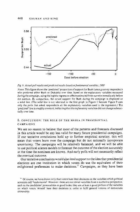
-1 50 -100 -50 0 Days before election

Fig. 9. Actual poll results andpredicted results based on fundamental variables, 1988

Notes: This figure shows the 'predicted' proportion of support for Bush (among survey respondents who preferred either Bush or Dukakis) over time, based on the explanatory variables measured during the campaign, using the logistic regression effects estimated from surveys immediately before the election. By comparison, the actual support for Bush during the campaign is displayed as a solid line. (The solid line is not identical to the first graph in Figure 1 because Figure 9 uses only the polls that asked respondents all the explanatory variables used in the regression.) The 'predicted' line is roughly constant, indicating that theexplanatory variables did not change substantially over time.

6. C O N C L U S I O N : T H E R O L E O F T H E M E D I A I N P R E S I D E N T I A L

C A M P A I G N S

We see no reason to believe that most of the patterns and forecasts discussed in this article would be any less valid for many future presidential campaigns. If our tentative conclusions hold up to further empirical scrutiny, this will mean that voters learn over the campaign but do not rationally incorporate uncertainty. The campaigns will be relatively balanced, and we will be able to use political science models to forecast the outcome of the election accurately at the time the nominees are known. And early polls will not necessarily reflect the eventual outcome.

Our tentative conclusions would also lend support to the idea that presidential elections are one institution in which voters do use the equivalent of their enlightened preferences to make decision^.^' Campaigns, as they have been

Of course, we have shown only that voters base their decisions on the variables which political scientists call 'fundamental'. However, these are not trivial variables from a normative perspective, such as the candidates' personalities or good looks; they are at least a good portion of the variables on which voters 'should' base their decisions in order to fulfil general notions of democratic citizenship.


run, are very important in producing this result. Underlying the puzzle of the title of this article is the following paradox: because of their central and relatively balanced role, presidential general election campaigns produce no unexpected advantage for their political party and are not necessary for forecasting.

What specific roles, then, do the campaign and the media have? The most important role, from this perspective, is to enlighten the voters - to give them sufficient information in a timely fashion so they can make up their minds relatively easily. The media can continue to make the campaign relatively fair by giving both candidates a reasonable opportunity to express their views, thus continuing to help inform the voters. All this will assist in making voters aware of where the candidates stand, and help them learn the values of their fundamental variables and their appropriate weights. Information about candidates' positions on issues is therefore the most important role of the media, and it should hardly be controversial (or novel) to suggest that they spend more time on it. All of our forecasting models require that voters know where the candidates stand, so this will also not change our ability to forecast. More- over, even though more attention to informing voters by the media will probably not change the outcome of the election, it would not hurt to improve the level of 'enlightened deliberation' during the campaign. Issues and proposed solutions do get raised and discussed, and increasing the level of explicit voter knowledge about these issues (which is currently quite low) could only improve the odds of reaching consensus among elected representatives.

Finally, journalists should realize that they can report the polls all they want, and continue to make incorrect causal inferences about them, but they are not helping to predict or even influence the e le~ t ion . '~ Journalists play a critical role in enabling voters to make decisions based on the equivalent of explicitly enlightened preferences. Unfortunately, by focusing more on the polls and meaningless campaign events, the media are spending more and more time on 'news' that has less and less of an effect.

The public opinion horse race of the early general election is of tremendous popular interest, so one can hardly blame the media for focusing on it so much. Perhaps the research presented here might help the media, and eventually citizens, to realize that winning this early 'race' is worth nothing: it does not help with the election; and it does not even help the candidates raise money (since general elections for president are now publicly funded). Because being ahead in the early polls is worth almost nothing, perhaps journalists and then the public will understand that the polls are not worthy of as much attention as they get. Do we really need to spend so much public attention on which horse gets into the starting booth first?

56 Reporting the polls does not seem to influence the outcome, since there is no evidence of a 'halo effect' - the winner in the early polls does not inevitably win the election - although it may work strongly in primaries.

A P P E N D I X

The forty-nine national public opinion polls we used are listed in Table 2 with the polling organization, the number of days before the election on which the survey took place and the sample size. We used all these surveys at different times in the analysis, but some analyses only used a subset of surveys (primarily CBS and ABC) due to the frequency with which various survey questions were asked. In all analyses, we weighted respondents by the survey weights supplied by the respective polling organizations.

T A B L E 2 Individual-Level Presidential Campaign Polls in 1988

Days Polling Days Polling Days Polling before organi- before organi- before organi-

election* zationt n election* zation? n election* zation? n$

-183 CBS - 178 Roper -173 ABC -146 ABC -139 AP -126 CBS -126 LAT -125 ABC -122 Roper -114 ABC -111 ABC - 110 Gallup -86 ABC -85 ABC -83 ABC -82 ABC -82 Gallup

CBS Harris

AP Roper L AT CBS ABC Yank CBS ABC

Harris LAT LAT CBS ABC

Harris CBS

Gallup Gallup

CBS Yank Harris Roper CBS CBS CBS CBS CBS CBS Yank CBS CBS

* Number of days before the 1988 presidential election. For reference, the Democratic convention began at - 114 and ended at - 11 I, and the Republican convention ran from- 86 to - 82. t Polling organizations are Harris, Yankelovich, CBSNew York Times, ABCiWashington Post, LA Times, Associated PressiMedia General, Roper, or Gallup. S'n' is the sample size, including undecided voters.

The figures use the following coding schemes for individual-level responses. For Vote, we use the respondent's preference for the Democratic or Republican ticket when available and otherwise for the Democratic or Republican presidential candidate. The most typical question wording can be found in the notes to Figure 2. Those who report leaning towards one party or another are not included. (We have found that including or excluding 'leaners' has little effect on our results.)

For Education, 'low' refers to a respondent with no college, and 'high' is one with some college experience (including those who fail to graduate). For logistic regression effects, the shift we use is from those with less than a high school diploma to those with some college. For Race, we use white vs. non-white for the two-way graphs and, in the logistic regression, use the shift from black (non-Hispanic) to white. Party is coded in three categories for the two-way graphs: Republican, Democratic and a third category consisting of Independents, no answer and those who prefer minor parties.


V) Party identification

=1 1.0 , , 2 1.0 Republicans 0,

u 0.8

P V)

g 0.6 g 0.6 +- +- 0 0 5 0.4 c 0.4

0

Democrats 0 0

c i 0.0 -150 -100 -50


Ideology

conservatives

J I

-150 -100 -50 Days before election

Fig. 10. Constancy ofparty identification and ideology over time, 1988

Notes: This figure plots party identification and ideology (as declared by respondents) over the course of the campaign. As can be seen, these vary very little and considerably less than variations in candidate preference. In addition, but not shown on this graph, the no-opinion rates for these two questions showed no trend during the campaign.

The logistic regression first differences represent shifts from Democratic to Republican. Region of the country is coded as northeast, midwest, south and west, and the logistic

regression differences are south vs. non-south. Ideology for graphs with two-way groups is coded in three categories: (1) very conservative, conservative, moderate-conservative; (2) moderate, others, no answer; (3) moderate-liberal, liberal, very liberal. In the logistic regression, the shift is from liberal to conservative.

Income for the graphs with two-way groups is broken into four categories: less than $1 5,000, $10,000-$25,000, $20,000-$50,000, and more than $50,000. The categories over- lap slightly because of discrete reporting. For the logistic regressions, the shift is from $10,000 to $40,000.

Finally, Figure 10 plots party identification and ideology over the course of the campaign. As can be seen, these vary very little, and considerably less than variations in candidate preferences. We therefore conclude with most of the literature on this subject that these variables are close to exogenous with respect to survey respondent support for presidential candidate^.^^

5 7 For example, Franklin and Jackson, 'The Dynamics of Party Identification'.

why are american presidential election campaign polls …gking.harvard.edu/files/bj215.pdf · why...

Documents