Whatever it takes: The Real E↵ects of

Unconventional Monetary Policy

Viral V. Acharya, Tim Eisert, Christian Eufinger, and Christian Hirsch

Abstract

On July 26, 2012 the ECB’s president Mario Draghi announced to do “whatever

it takes” to preserve the Euro and subsequently launched the Outright Monetary

Transactions (OMT) Program, which led to a significant increase in the value of

sovereign bonds issued by European periphery countries. As a result, the OMT an-

nouncement indirectly recapitalized periphery country banks due to their significant

holdings of these bonds. However, the regained stability of the European banking

sector has not fully transferred into economic growth. We show that this develop-

ment can at least partially be explained by zombie lending motives of banks that

still remained undercapitalized after the OMT announcement. While banks that

benefited from the announcement increased their overall loan supply, this supply

was mostly targeted towards low-quality firms with pre-existing lending relation-

ships with these banks. As a result, there was no positive impact on real economic

activity like employment or investment. Instead, these firms mainly used the newly

acquired funds to build up cash reserves. Finally, we document that creditworthy

firms in industries with a prevalence of zombie firms su↵ered significantly from the

credit misallocation, which slowed down the economic recovery.

The authors appreciate helpful comments from Taylor Begley, Luc Laeven, Steven Ongena, SaverioSimonelli, Marti Subrahmanyam, and Annette Vissing-Jorgensen. Furthermore, we thank conferenceparticipants at the Third Conference on Sovereign Bond Markets, the Sixteenth Jacques Polak AnnualResearch Conference, and the CEPR/RELTIF Meeting in Milan as well as seminar participants at Utah,Rutgers, the European Central Bank, Rotterdam, Leuven, the Austrian Central Bank, Amsterdam, andFrankfurt. We are grateful to the Assonime/ CEPR Research Programme on Restarting European Long-Term Investment Finance (RELTIF) for financial support of the research in this paper. Hirsch gratefullyacknowledges support from the Research Center SAFE, funded by the State of Hessen initiative forresearch Loewe. Eufinger gratefully acknowledges the financial support of the Public-Private SectorResearch Center of the IESE Business School, as well as, the Europlace Institute of Finance (EIF) andthe Labex Louis Bachelier. Corresponding author: Viral V. Acharya, Phone: +1-212-998-0354, Fax:+1-212-995-4256, Email: vacharya@stern.nyu.edu, Leonard N. Stern School of Business, 44 West 4thStreet, Suite 9-84, New York, NY 10012.

New York University, CEPR, and NBERErasmus University RotterdamIESE Business SchoolGoethe University Frankfurt and SAFE

1 Introduction

At the peak of the European debt crisis in 2010, the European Central Bank (ECB)

began to introduce unconventional monetary policy measures to stabilize the Eurozone

and restore trust in the periphery of Europe. Ultimately, these unconventional monetary

policy measures were aimed at breaking the vicious circle between poor bank health

and sovereign indebtedness, which had led to a sharp decline in economic activity in

the countries in the periphery of the Eurozone (Acharya, Eisert, Eufinger, and Hirsch,

2015). Especially important in restoring trust in the viability of the Eurozone was the

ECB’s Outright Monetary Transactions (OMT) program, which the ECB’s president

Mario Draghi announced in his famous speech in July of 2012, saying that “[...] the ECB

is ready to do whatever it takes to preserve the euro. And believe me, it will be enough.”

Once activated towards a specific country, the OMT program allows the ECB to buy a

theoretically unlimited amount of the country’s government bonds in secondary markets.

There is clear empirical evidence that the announcement of the OMT program has been

successful in terms of lowering spreads of sovereign bonds issued by distressed European

countries (e.g., Krishnamurthy, Nagel, and Vissing-Jorgensen, 2014). Moreover, we show

that the resulting value increase of these bonds resulted in a backdoor (indirect) bank

recapitalization as banks with significant holdings of these bonds experienced substantial

windfall gains, which helped to restore the stability of the European banking system (see

also Acharya, Pierret, and Ste↵en, 2015).1

However, when Mario Draghi reflected on the impact of the OMT program on the

real economy during a speech in November 2014, he noted that “[...] these positive de-

velopments in the financial sphere have not transferred fully into the economic sphere.

The economic situation in the euro area remains di�cult. The euro area exited recession

in the second quarter of 2013, but underlying growth momentum remains weak. Unem-

ployment is only falling very slowly. And confidence in our overall economic prospects is

fragile and easily disrupted, feeding into low investment.”

There are a lot of unvital signs that Europe’s weak economic recovery is a repeat

of Japan’s “zombie lending” experience in the 1990s, when banks in distress failed to

foreclose on unprofitable and highly indebted firms.2 For example, in 2013, in Portugal,

Spain and Italy, 50%, 40% and 30% of debt, respectively, was owed by firms which were

not able to cover their interest expenses out of their pre-tax earnings.3 To the best of our

knowledge, our paper is the first to provide systematic evidence that, indeed, the slow

1The OMT program has in particular recapitalized the banks that caused the loan supply disruptionsduring the European debt crisis. Confirming the positive e↵ect of the indirect recapitalization, wefind that the CDS spreads of these banks decreased significantly on the dates surrounding the OMTannouncement.

2See, for example, “Blight of the living dead”, The Economist, July 13, 2013 and “Companies: Therise of the zombie” by Michael Stothard, Financial Times, January 8, 2013.

3“Europe’s other debt crisis”, The Economist, October 26, 2013.

1

economic growth in Europe can at least partially be explained by zombie lending motives

of banks that still remained undercapitalized after the OMT announcement.

While an indirect recapitalization measure like the OMT program allows central banks

to target the recapitalization to banks holding troublesome assets, it does not allow them

to tailor the amount of the recapitalization to a bank’s specific capital needs. Therefore,

even though European banks regained some lending capacity due to the recapitalization

e↵ect of the OMT announcement, some of these banks still remained weakly-capitalized

after the announcement, creating zombie lending incentives for these banks. By contin-

uing to lend to their impaired borrowers, distressed banks can avoid realizing losses on

outstanding loans, which would further deter the banks’ situation due to increasing reg-

ulatory scrutiny and intensified pressure from market forces. Instead, by “evergreening”

loans to their impaired borrowers, banks in distress can gamble for resurrection in the

hope that their borrowers regain solvency, or, at least, they can delay taking a balance

sheet hit. This behavior leads to an ine�cient allocation of bank loans, since loan supply

is shifted away from creditworthy productive firms towards distressed less productive bor-

rowers, which distorts market competition and causes detrimental e↵ects on employment,

investment, and growth in general.4

Our sample is based on loan information data obtained from Thomson Reuters LPC’s

DealScan, which provides extensive coverage of bank-firm relationships throughout Eu-

rope. We augment this dataset with firm-specific information from Bureau van Dijk’s

Amadeus database and bank-specific information from various sources, including the

banks’ CDS spreads, balance sheet information, and sovereign debt holdings. The sam-

ple includes all private firms from all EU countries for which Dealscan provides loan

information and covers the years 2009 until 2014. This dataset allows us to trace the im-

pact of the OMT program announcement through the banking sector to the real economy.

Accordingly, we organize our empirical analysis into three parts. First, we determine the

extent to which individual banks were a↵ected by the announcement of the OMT pro-

gram. Second, we track the resulting change in their lending behavior and, finally, we

evaluate whether the change in loan supply led to real e↵ects for European firms.

Our results show that banks from stressed European countries (the GIIPS countries,

i.e., Greece, Ireland, Italy, Portugal, and Spain) realized the highest windfall gains after

the OMT announcement due to their substantial amount of sovereign debt holdings from

these countries. Moreover, we document that this increase in bank health led to an

increase in available loans to firms. Building on the methodology of Khwaja and Mian

(2008), we find that, in the quarters following the OMT announcement, banks with higher

windfall gains on their sovereign debt holdings increased loan supply to the corporate

sector relatively more than banks with lower windfall gains, but only to existing borrowers

4See Kane (1989), Peek and Rosengren (2005), Caballero, Hoshi, and Kashyap (2008), and Giannettiand Simonov (2013).

2

(intensive margin). Conversely, we do not find any significant relation between a bank’s

windfall gains and its propensity to issue new loans to borrowers it did not have a prior

relation with (extensive margin).

To analyze which type of borrowers benefited most from an increased lending volume

in the period after the announcement of the OMT program, we divide our sample into

low- and high-quality borrower based on the ability of firms to service existing debt. In

particular, a low-quality (high-quality) borrower is defined as having a below (above)

country median interest coverage ratio. The results of our lending regressions show that

in particular low-quality borrowers benefited from the increased loan volume in the period

following the OMT program announcement. In contrast, high-quality borrower did not

benefit significantly from the OMT announcement as the loan volume extended to this

subset of firms did not increase. The fact that the banks’ loan supply increase in the

period following the OMT announcement was primarily targeted towards existing low-

quality borrowers is a first indication that zombie lending behavior might have prevailed

in the European lending market.

Given this evidence, we then specifically test whether these results can indeed be

traced back to zombie lending behavior by banks that regained some lending capacity due

to the OMT announcement but still remained weakly-capitalized. Following Caballero,

Hoshi, and Kashyap (2008) and Giannetti and Simonov (2013), we show that these banks

extended loans to existing low-quality borrowers at interest rates that are below the rates

paid by the most creditworthy European borrowers (high-quality public borrowers in non-

GIIPS European countries). Lending at these very advantageous interest rates is a very

strong indication that the banks’ lending behavior can at least partially be explained by

zombie lending motives.

In a next step, we determine how the change in the banks’ lending behavior, induced

by the OMT announcement, has impacted corporate policies of firms. For this analysis,

we closely follow the approach used in Acharya, Eisert, Eufinger, and Hirsch (2015).

In particular, we use a di↵erence-in-di↵erences framework to evaluate the performance

and policies of borrowing firms in the post-OMT period. To measure the impact of the

OMT program announcement, we construct a variable for each firm that captures its

indirect benefits from the post-OMT value increase of the sovereign debt holdings of the

banks it is associated with. We provide evidence that borrowers with higher indirect

OMT windfall gains (that is, benefits were accrued via their banks) increased both their

cash holdings and leverage by roughly the same amount, suggesting that they used the

majority of cash inflow to build up cash reserves. Firms that received subsidized loans

(zombie firms), on the other hand, are not able to increase cash and leverage by the

same margin since these firms have to use the funds acquired through new loans, at

least partially, to repay some other debts. Moreover, we do not find any changes in real

economic activity: neither investment, employment, nor return on assets are significantly

3

a↵ected by a firms’ indirect OMT windfall gains.

To consistently estimate the real e↵ects for borrowing firms, we include industry-

country-year fixed e↵ects to capture any time-varying shocks to an industry in a given

country that may have a↵ected the firms’ credit demand, their access to credit, and/or

their real outcomes. Moreover, if a firm borrows from a bank incorporated in a GIIPS

country (GIIPS bank), we include foreign bank GIIPS country-year fixed e↵ects, that is,

a fixed e↵ect for the GIIPS bank’s country of incorporation. These fixed e↵ects absorb

any unobserved, time-varying heterogeneity that may arise because a firm’s dependency

on banks from a certain country might be influenced by whether this firm has business in

the respective country. Consider as an example a German firm borrowing from a Spanish

and a German bank. For this firm, we also include a Spain-year fixed e↵ect to capture the

firm’s potential exposure to the economic downturn in Spain during the sovereign crisis.

Furthermore, we control for unobserved, time-constant firm heterogeneity and observable

time-varying firm characteristics that a↵ect the firms’ corporate policies, loan demand,

and/or loan supply.

In a final step, we analyze whether the rise in zombie firms after the OMT announce-

ment had an impact on non-zombie firms operating in the same industries. There are two

potential channels through which non-zombie firms could be negatively a↵ected. First,

banks with zombie lending incentives might shift their loan supply to existing distressed

borrowers, thereby crowding-out credit to productive creditworthy firms operating in

the same industries. Second, zombie lending keeps distressed borrowers artificially alive,

which congests the respective markets. The resulting distorting e↵ects on healthy firms

competing in the same industries include, for example, depressed product market prices

and higher market wages. Building on the analysis of Caballero, Hoshi, and Kashyap

(2008), we document that high-quality non-zombie firms indeed su↵ered from the pres-

ence of zombie firms in their industry: both their investment and employment growth

rates were significantly lower if the fraction of zombie firms in their industry increased

compared to high-quality non-zombie firms active in industries without a high prevalence

of zombie firms. This finding highlights that the distorted market competition, induced by

the misallocation of loan supply due to zombie lending, hampered real economic growth

and thus significantly weakened the potentially positive impact of the OMT program’s

indirect bank recapitalization e↵ect.

Therefore, our analysis provides evidence that central banks can indirectly recapitalize

an undercapitalized banking sector by a↵ecting the prices of assets that banks are holding

on their balance sheets. However, it also highlights that central banks need to pay close

attention to the magnitude of the gains that banks can realize from their intervention,

and hence the amount of additional equity capital these banks are being provided. If the

backdoor (indirect) bank recapitalization fails to adequately recapitalize (some) banks,

zombie lending incentives may arise, which can have detrimental e↵ects on employment,

4

investment, and growth in general.

Overall, the announcement of the OMT program probably averted an even fiercer

economic downturn or even a break-up of the Eurozone. Our results suggest, however,

that combining the OMT program with a targeted bank recapitalization program would

presumably have led to superior outcomes in terms of economic growth. Given a well-

capitalized European banking system, the increased loan supply would have been targeted

mainly at the most productive firms and, without the market distortions due to zombie

lending, the regained stability of the European banking system probably would have been

fully transferred into economic growth.

2 Outright Monetary Transactions

In mid-2012 the anxiety about excessive national debt led to interest rates on Italian

and Spanish government bonds that were considered unsustainable. From mid-2011 to

mid-2012, the spreads of Italian and Spanish 10-year government bonds had increased by

200 and 250 basis points, respectively relative to German government bonds. As a result,

yields on 10-year Italian and Spanish government bonds were more than 4 percentage

points higher than yields on German government bonds in July 2012.

This significant increase in bond spreads of countries in the periphery of the Eurozone

became a matter of great concern for the ECB as it endangered the monetary union as

a whole. In response to the mounting crisis, ECB President Mario Draghi stated on

July 26, 2012, during a conference in London: “Within our mandate, the ECB is ready

to do whatever it takes to preserve the euro. And believe me, it will be enough.” On

August 2, 2012, the ECB announced it would undertake outright monetary transactions

in secondary, sovereign bond markets. The technical details of these operations were

unveiled on September 6, 2012.

To activate the OMT program towards a specific country, that is, buy a theoretically

unlimited amount of government bonds with one to three years maturity in secondary

markets, four conditions have to be met. First, the country must have received financial

support from the European Stability Mechanism (ESM). Second, the government must

comply with the reform e↵orts required by the respective ESM program. Third, the

OMT program can only start if the country has regained complete access to private

lending markets. Fourth, the country’s government bond yields are higher than what

can be justified by the fundamental economic data. In case the OMT program would be

activated the ECB would reabsorb the liquidity pumped into the system by auctioning o↵

an equal amount of one-week deposits at the ECB. By Summer 2015, the OMT program

has still not been actually activated.

There is clear empirical evidence that the OMT announcement significantly lowered

5

sovereign bond spreads. For example, Szczerbowicz et al. (2012) find that the OMT mea-

sure lowered covered bond spreads and periphery sovereign yields. Altavilla, Giannone,

and Lenza (2014), Krishnamurthy, Nagel, and Vissing-Jorgensen (2014), and Ferrando,

Popov, and Udell (2015) reach a similar conclusion by showing that the OMT announce-

ments led to a relative strong decrease for Italian and Spanish government bond yields

(roughly 2 pp), while bond yields of the same maturity in Germany and France seem

una↵ected. Furthermore, Krishnamurthy, Nagel, and Vissing-Jorgensen (2014) investi-

gate which channels led to the reduction in bond yields. The authors find that for Italy

and Spain, a decrease in default and segmentation risks was the main factor in case of

OMT, while there might have been a reduction in redenomination risk in the case of

Spain and Portugal, but not for Italy. Finally, their paper shows that the announcement

of the OMT measure led to large increases in stock prices in both distressed and core

countries. Saka, Fuertes, and Kalotychou (2015) finds that the perceived commonality

in default risk among peripheral and core Eurozone sovereigns increased after Draghi’s

“whatever-it-takes” announcement.

The higher demand for GIIPS bonds and, in turn, higher bond prices implied that

banks were able to sell government bonds with a profit and bonds in the banks’ trading

book, which are marked to market, increased in value. Both improved the banks’ equity

position. For example, Italian-based UBI Banca states in its annual report of 2012:“The

e↵ects of the narrowing of the BTP/Bund spread entailed an improvement in the market

value of debt instruments with a relative positive net impact on the fair value reserve of

Euro 855 million [...].” Given UBI Banca’s total equity of 8,608 million, this amounts to a

gain of 9.9% of total equity. Consistent with this statement, Krishnamurthy, Nagel, and

Vissing-Jorgensen (2014) and Acharya, Pierret, and Ste↵en (2015) document significantly

positive e↵ects on banks’ equity prices after the OMT announcement.

Moreover, due to the lower sovereign bond spreads and the resulting positive e↵ect

on the banks’ financial stability, investors regained faith in the banking sectors of the

stressed countries. This improved the ability of banks from GIIPS countries to acquire

funding from financial markets. For example, Spain-based BBVA noted in its annual

report of 2012: “[...] as a result of new measures adopted by the ECB with the outright

monetary transactions (OMT), the long-term funding markets have performed better,

enabling top-level financial institutions like BBVA to resort to them on a recurring basis

for the issue of both senior debt and covered bonds.” Furthermore, since banks regularly

use sovereign bonds as collateral, their access to private repo markets and ECB financing

improved as well due to higher bond ratings and the resulting lower haircuts.

Hence, by substantially reducing sovereign yields, the OMT program improved the

asset side, capitalization, and ability to access financing for banks with large GIIPS

sovereign debt holdings, and thereby the financial stability of these banks. However, there

is still no conclusive evidence about the impact of the regained financial stability of the

6

European banking sector, induced by the ECB’s OMT program, on bank lending and the

resulting e↵ects for the real economy. To our knowledge, our paper and a concurrent paper

by Ferrando, Popov, and Udell (2015) are the only papers that investigate the e↵ects of

OMT on extension of credit to European borrowers. Using survey data, Ferrando, Popov,

and Udell (2015) find that after the announcement of OMT, less firms report that they

are credit rationed and discouraged from applying for loans. While we also study the

impact of the OMT announcement on bank lending, we additionally provide evidence for

zombie lending behavior and analyze the consequence of the OMT announcement on the

real economy.

3 Data

We use a novel hand-matched dataset that contains bank-firm relationships in Europe,

along with detailed firm and bank-specific information. Information about bank-firm re-

lationships are taken from Thomson Reuters LPC’s DealScan, which provides a compre-

hensive coverage of the European syndicated loan market. In contrast to the U.S., bank

financing is the key funding source for firms in our sample since only very few bonds are

issued in Europe (Standard&Poor’s, 2010). The sample includes all private firms from all

EU countries for which Dealscan provides loan information and our sample period spans

the fiscal years 2009-2014. Consistent with the literature (e.g., Sufi, 2007), all loans are

aggregated to a bank’s parent company.

We augment the data on bank-firm relationships with firm-level accounting data taken

from Bureau van Dijk’s Amadeus database. This database contains information about

19 million public and private companies from 34 countries, including all EU countries.5

Since especially non-listed firms were a↵ected by the lending contraction in the periphery

due to their lack of alternative funding sources, we restrict our sample to private firms

in Europe (see Acharya, Eisert, Eufinger, and Hirsch (2015)). This allow us to evaluate

whether firms that were under severe stress during the peak of the sovereign debt crisis

benefited from the OMT announcement.

Finally, we obtain information on bank as well as sovereign CDS spreads from Markit,

bank equity and sovereign bond information from Datastream, bank level balance sheet

data from SNL, and data on the sovereign debt holdings of banks from the EBA stress

tests, transparency, and capital exercises. For banks to be included in the sample, they

must act as lead arranger in the syndicated loan market during our sample period. We

identify the lead arranger according to definitions provided by Standard & Poor’s, which

for the European loan market are stated in Standard & Poor’s Guide to the European

loan market (2010). Therefore, we classify a bank as a lead arranger if its role is either

5For a description of the process to match DealScan and Amadeus see Acharya, Eisert, Eufinger,and Hirsch (2015).

7

“mandated lead arranger”, “mandated arranger”, or “bookrunner”. Moreover, the bank

needs to be included in EBA stress tests and must have data about the sovereign bond

holdings available prior to the OMT announcement (June 2012).

4 Results

4.1 Bank Health

We begin our empirical analysis by investigating the e↵ect of the OMT announcement

on the financial health of large European banks. We conduct an event study using CDS

spreads that we compile from Markit. For the OMT announcement dates, we follow

Krishnamurthy, Nagel, and Vissing-Jorgensen (2014) and analyze the events on July 26,

2012 (“whatever-it-takes” speech); August 2, 2012 (announcement of the OMT program;

and September 6, 2012 (announcement of technical details).

In 2012, financial markets throughout Europe were characterized by tensions and high

uncertainty. We account for these market conditions in our analysis by, first, using a 1-

day event window in our event study.6 By employing a narrow window around the OMT

announcement dates, we are able to separate the e↵ect of the OMT announcement from

other events that may potentially influence financial bank health. Second, we follow the

time-series event study approach of Krishnamurthy and Vissing-Jorgensen (2011), which

compares the event announcement period (OMT in our case) to other periods of the same

length without an event. The advantage of this approach is that it does account for the

possibility that other events may arrive during the OMT announcement periods. In doing

so the estimated standard errors are more conservative than standard errors from a more

traditional cross sectional event study.

Results are presented in Panel A of Table 1. Column (1) reports results for time-series

regressions of CDS spreads on a set of dummy variables for the three OMT announcement

dates. We run separate regressions for the subset of GIIPS and non-GIIPS banks and

report the mean of the sum over the three event dates. The CDS spread of the mean GIIPS

bank decreased by -96bp over the three OMT announcement dates, while it decreased by

-23bp for the average non-GIIPS bank.

To gauge the statistical significance, we conduct F-tests of the joint significance of

the dummy variables in our time-series regressions. The F-test is reported in parenthesis

below the mean and indicates that the CDS spreads on days with OMT announcements

are jointly significantly di↵erent from zero for both subsets of banks. To gauge the

di↵erence in the magnitude of the announcement e↵ects for the two subsets, we use a

t-test for the di↵erence in means. The test shows that the default risk of GIIPS banks

6Results from a 2- or 3-day event window are qualitatively and quantitatively similar.

8

decreased by a larger margin than the default risk of non-GIIPS banks.

We draw two main conclusions from this result. First, the OMT announcement led

to an improvement of bank financial health for all European banks, that is, for GIIPS

and non-GIIPS banks, as evidenced by a substantial decrease in CDS spreads. Second,

the e↵ect of the OMT announcement for GIIPS banks is about four times larger than

the e↵ect for non-GIIPS banks.

To analyze the large di↵erence in the magnitude of the CDS return between non-

GIIPS and GIIPS banks, we exploit information on EU sovereign debt holdings of banks

directly. In particular, we use changes in sovereign bond prices, as well as information on

sovereign debt holdings, to estimate the impact of the OMT program announcement on

the value of the banks’ sovereign debt holdings. Since a large fraction of these holdings

are held in the banks’ trading books, and are hence marked to market, an increase in

their value translates into an equity capital gain for the banks. We call this variable the

OMT windfall gain. Note that, while mainly GIIPS sovereign yields were a↵ected by the

OMT announcement, the sovereign yields of other countries were also a↵ected (although

to a lesser extent). To capture all sovereign debt holdings, our measure of OMT windfall

gain is based on all EU sovereign debt holdings of a bank.

To compute the OMT windfall gain, we first compile data on the sovereign debt hold-

ings of all sample banks at the closest date before July 26 (the first OMT announcement

date) from the EBA webpage.7 From Datastream, we obtain information on EU sovereign

bonds prices, yields, and duration for various maturities. Second, we calculate the change

in bond prices for all maturities around the three OMT announcement dates (July 26, Au-

gust 2, and September 6) and sum these changes across the three announcement dates.8

Third, we multiply the respective sovereign debt holdings outstanding before July 26 and

the sum of the change in sovereign bond prices for each maturity and country with valid

bond price information in Datastream. Finally, the total OMT windfall gain follows from

summing the individual gains over all EU sovereign bonds in the banks portfolio. We re-

port this gain on sovereign debt holdings as a fraction of a bank’s total equity throughout,

that is, we define the windfall gains of bank b in country j as:

OMT windfall gainbj =�Value EU Sov. Debt bj

Total Equitybj

. (1)

Note that, similar to Krishnamurthy, Nagel, and Vissing-Jorgensen (2014), we are only

able to use sovereign yields from three out of the five GIIPS countries (Spain, Italy, and

Portugal), since for Greece and Ireland information on yields is partially or completely

missing. Since the majority of sovereign debt holdings of GIIPS banks is domestic, we

7Sovereign debt holdings are from June 2012.8As a robustness check, we compute the change in bond prices by using the duration of a bond and

the change in yield, where the change in yield is either computed from Datastream yields or taken fromKrishnamurthy, Nagel, and Vissing-Jorgensen (2014). Results do not change.

9

are not able to calculate the OMT windfall gain for Greek and Irish banks in our sample,

since we cannot derive the gain in value of their sovereign debt holdings.

Column (2) of Panel A in Table 1 reports the results for the OMT windfall gain,

split by GIIPS and non-GIIPS banks. Both subsets of banks experienced significant

windfall gains from the appreciation of value of their sovereign debt portfolio through the

announcement of the OMT program. However, when testing the di↵erence between the

two subgroups, perhaps not surprisingly, GIIPS banks experienced significantly larger

windfall gains compared to non-GIIPS banks as is evidenced by a t-value of 5.69. This

significant di↵erence is due to the fact that banks’ sovereign banks holdings are biased

towards their own domestic sovereign (e.g., Acharya and Ste↵en, 2014) and that GIIPS

sovereign yields were most a↵ected by the OMT announcement.

Column (3) of Panel A in Table 1 shows that the value of GIIPS sovereign bond

holdings reported to the EBA right before the announcement of the OMT program as a

fraction of total assets is roughly 10 times larger for GIIPS banks than for non-GIIPS

banks (11.8% compared to 1%). Therefore, as mainly GIIPS sovereign debt appreciated

in value in response to the OMT measure, GIIPS banks benefited much more from the

OMT program than non-GIIPS banks. Consistent with this explanation, Figure 1, Panel

A shows a clear negative relation between a bank’s sovereign debt holdings and its CDS

return around the OMT announcement. This relation is also present within the subsample

of GIIPS banks, as shown by Figure 1, Panel B.

Panel B of Table 1 presents the evolution of the banks’ book leverage ratio separately

for GIIPS banks and non-GIIPS banks as well as for U.S. banks. We split GIIPS banks

further into banks have an above median leverage ratio after the OMT announcement

(still undercapitalized) and those with a below median leverage ratio (well-capitalized).

Before the start of the financial and sovereign debt crisis, both well-capitalized and still

undercapitalized GIIPS banks had lower leverage ratios than non-GIIPS banks. But while

the leverage ratio decreased significantly over time for non-GIIPS banks, it increased

dramatically (peaking in the year prior to the OMT announcement at 24.74) for GIIPS

banks classified as still undercapitalized and slightly for well-capitalized GIIPS banks over

the sovereign debt crisis period. While the the leverage ratio of weakly-capitalized GIIPS

banks improved significantly (by around 15% in total) after the OMT announcement, they

still remain highly levered after the announcement. Well-capitalized GIIPS banks, on the

other hand, are back to their pre-crisis leverage ratio after the OMT announcement. A

similar picture emerges when considering the quasi leverage of banks, defined as market

value of equity plus the book value of debt divided by the market value of equity (see

Panel C of Table 1).

Next, we provide detailed evidence on how much of the change in CDS spreads around

the OMT announcements can be explained by banks’ sovereign debt holdings and their

resulting windfall gains. In particular, we regress the value of the GIIPS sovereign debt

10

holdings of banks and the OMT windfall gain on a bank’s CDS return. We compute the

change in CDS spread for each bank by summing CDS spread changes over the three

OMT announcement dates.

Results are presented in Table 2. Panel A reports results for the value of the GIIPS

sovereign debt holdings of banks. In all specifications, this variable has a significantly

negative e↵ect on a bank’s CDS return, suggesting that banks indeed benefited through

the increase in the value of their sovereign debt holdings (which is in line with the finding

of Acharya, Pierret, and Ste↵en, 2015). Panel B of Table 2 documents a similar pattern

for the OMT windfall gain variable.

To summarize, we find evidence which is consistent with the OMT announcement

increasing the financial health of large banks in Europe. The e↵ect is larger for GIIPS

banks, which are the banks that had reduced their lending volume to the real sector

during the sovereign debt crisis. We show that an important channel of the mechanism

works through GIIPS sovereign debt holdings of banks.

4.2 Bank Lending

We now turn to the question of whether the increased health of periphery country

banks with high GIIPS sovereign debt holdings led to an increase in loan supply in the

quarters following the OMT announcement and if so which borrowers benefited the most.

We employ the same methodology as Acharya, Eisert, Eufinger, and Hirsch (2015) to

control for loan demand and other observed and unobserved changes in borrowing firm

characteristics. In particular, we track the evolution of the lending volume from a specific

bank to a certain firm cluster, which allows us to control for any observed and unobserved

characteristics that are shared by firms in the same cluster and that might influence loan

outcomes.

To this end, we form firm clusters based on the following three criteria, which capture

important drivers of loan demand, as well as the quality of firms in our sample: (1) the

country of incorporation; (2) the industry; and (3) the firm rating. The main reason

for aggregating firms based on the first two criteria is that firms in a particular industry

in a particular country probably share a lot of firm characteristics and were thus likely

a↵ected in a similar way by macroeconomic developments during our sample period.

Our motivation behind forming clusters based on credit quality follows from theoretical

research in which credit quality is an important source of variation driving a firm’s loan

demand (e.g., Diamond (1991)).

Since we focus on private borrowers, firms in our sample generally do not have a

credit rating. To aggregate firms into clusters, we assign ratings estimated from interest

coverage ratio medians for firms by rating category provided by Standard & Poor’s. This

approach exploits the fact that our measure of credit quality which is based on accounting

11

information is monotone across credit categories. We follow Standard & Poor’s and assign

ratings on the basis of the three-year median interest coverage ratio of each firm.

We start our empirical investigation by analyzing the supply of bank loans to private

borrowers around the OMT announcement graphically. Figure 2 plots the log of the sum

loans provided by banks that strongly benefited (above median OMT windfall gain) and

banks that benefited less (below median OMT windfall gain) from the OMT announce-

ment in a given quarter. Note that we measure the change in loan volume relative to the

quarter of the OMT announcement, that is, the y-axis is normalized to zero at the time of

the announcement in Q3 2012. Figure 2 documents a significant increase in loan supply

by banks that strongly benefited from the OMT announcement to private borrowers after

Q3 2012. In contrast, we do not see a similar increase in loan supply by banks that did

not significantly benefit from the measure. Furthermore, the figure shows that, pre-OMT

announcement, the bank loan supply by banks with a low OMT windfall gain is higher

than that by banks with a high OMT windfall gain (which are mostly GIIPS banks), a

result confirmed by previous studies (e.g., Acharya, Eisert, Eufinger, and Hirsch, 2015).

In the following we investigate both, whether high OMT windfall gain banks increase

loan supply to existing borrowers (intensive margin) and whether they have a higher

propensity to grant new loans to borrowers with which no relation existed in the period

before the OMT announcement (extensive margin). Our preferred specification to esti-

mate the quarterly change in loan volume provided by bank b in country j to firm cluster

m in quarter t (intensive margin) is given by:

�V olumebmjt+1 = �1 ·OMT windfall gainbj ⇤ PostOMT

+ � ·Xbjt + Firm Clusterm ·Quarter-Year t+1

+ Firm Clusterm · Bank bj + ubmjt+1, (2)

where OMT windfall gain is as defined in Eq. (1). Note that the firm clusters in this

case only consist of firms that had a prior relation (before the OMT announcement) with

a bank.

For the extensive margin our dependent variable is an indicator equal to one if the

bank issued a new loan to a firm cluster to which no relation existed in the period prior

to the OMT announcement. Our specification is given by:

NewLoanbmjt+1 = �1 ·OMT windfall gainbj ⇤ PostOMT

+ � ·Xbjt + Firm Clusterm ·Quarter-Year t+1

+ Firm Clusterm · Bank bj + ubmjt+1. (3)

Here firm clusters consist of firms with no prior relation (before the OMT announcement)

with a bank. We present the results of our empirical analysis in Table 3. As before, we

12

use a bank’s windfall gain on its sovereign debt portfolio from the OMT announcement

to proxy how much the bank benefited from the OMT program. Therefore, our main

variable of interest is OMT windfall gain interacted with a dummy variable PostOMT,

which is equal to one when the quarter falls into the period after the OMT announce-

ment. The results in Panel A show that banks with higher windfall gains from the OMT

announcement significantly increased their supply of bank loans to existing private bor-

rowers (intensive margin) after the OMT announcement across all specifications, which

control for di↵erent sets of fixed e↵ects. When we include bank and quarter-year fixed

e↵ects in our regression, the coe�cient on the interaction between OMT windfall gain

and PostOMT is positive and significant, as shown in Column (1).

This result continues to hold if we interact firm-cluster and bank fixed e↵ects. By

doing this, we exploit the variation within the same firm-cluster-bank relationship over

time. This controls for any unobserved characteristics that are shared by firms in the same

cluster, bank heterogeneity, and for relationships between firms in a given cluster and the

respective bank. The results of this specification are presented in Column (2). The

interaction between OMT windfall gain and PostOMT remains positive and significant.

Finally, in the results reported in Columns (3) and (4), we add firm-cluster-time fixed

e↵ects, which allow us to additionally control for any time observed and unobserved

time-varying characteristics that are shared by firms in the same cluster.

To further test the robustness of these results, we follow Peek and Rosengreen (2005)

and Giannetti and Simonov (2013) and employ the probability of a loan increase instead

of the change in the loan amount as the dependent variable in our regression analysis.

Results in Column (5) of Table 3 confirm that our result is invariant to using this alter-

native measure of lending supply expansion. Finally, Column (6) of Table 3 estimates

the regression when we restrict our sample to GIIPS banks. Recall that, in particular,

GIIPS banks hold large GIIPS sovereign debt holdings, which implies that especially

these banks benefited from the OMT program announcement. The significant coe�cient

in Column (6) shows that also within the subsample of GIIPS banks, those banks with

higher windfall gains increased lending to private borrowers more than GIIPS banks with

lower windfall gains.

Conversely, Panel C of Table 3 shows that there is no significant relation between a

bank’s OMT windfall gains and its propensity to issue a new loan to a group of borrowers

it had no prior relationship with. These results suggest that only existing borrowers

benefited from the loan supply increase induced by the OMT Program. As a robustness

check, we replace OMT windfall gain in the above regression with a bank’s CDS return

on the OMT announcement dates. This allows us to determine the extent to which

banks benefited from the OMT announcement with market price reactions and thus the

perceived change in bank credit risk in the market. Results are presented in Table A1 in

the online appendix. Panel A and B show that all results continue to hold qualitatively

13

and quantitatively using this alternative measure.

We now turn to analyzing which type of borrowers benefited most from an increased

lending volume in the period after the announcement of the OMT program. We identify

a low-quality (high-quality) borrower as a borrower with a below (above) country median

3-year average interest coverage ratio in the crisis years 2009 to 2011. The general picture

that emerges from Panel B in Table 3 is that the increase in loan volume (at the intensive

margin) in the period after the OMT announcement is entirely driven by low-quality

borrowers since only the triple interaction term of OMT windfall gains, post-OMT, and

low-quality is significantly positive.

An explanation for this result is that in many cases borrowers with a below country

median average interest coverage ratio based on the 2009 to 2011 period are precisely

those borrowers that had close borrowing relationships with GIIPS banks in the past.

Acharya, Eisert, Eufinger, and Hirsch (2015) show that, while not being less healthy

before the outbreak of the European sovereign debt crisis (i.e., there was no systematic

relation between firm quality and whether a firm borrowed from GIIPS banks prior to the

sovereign debt crisis), firms that were very dependent on GIIPS banks became financially

constrained during the sovereign debt crisis. This is due to the fact that GIIPS banks

were weakly-capitalized and decreased lending to the private sector. Since bank-borrower

relationships are sticky (Chodorow-Reich (2014)), and private firms are less able to utilize

alternative funding sources, these borrowers were stuck with weakly-capitalized banks.

This implies that they got under stress themselves and as a result their interest coverage

ratios decreased, as shown by Figure 6, Panel A. Panel D of Table 3 again confirms that

there are no significant loan supply e↵ects at the extensive margin, even if we split the

firms according to their quality. Panels C and D of Table A1 show that these results

continue to hold if we use the CDS return on the OMT announcement dates instead of

the OMT windfall gains.

Given this evidence that only low quality borrower benefited at the intensive margin,

we next explore whether banks’ lending behavior can be explained by loan evergreen-

ing (zombie lending). In particular, weakly-capitalized banks have an incentive to roll

over existing loans to distressed borrowers or even increase the lending volume to these

borrowers to avoid having to write down outstanding loans, which would mean that

banks have to realize large losses and thus dramatically worsen their situation. Indeed,

anecdotal evidence suggests that concerns over their balance sheet prevented banks from

restructuring their loan portfolio. An economist from a major bank said in this context:

“In Spain, Ireland, Portugal and Greece, banks have been reluctant to pull the plug on

companies as it would have forced them to crystallise heavy losses”.9

To detect zombie firms, we follow the approach in Caballero, Hoshi, and Kashyap

9“Companies: The rise of the zombie” by Michael Stothard, Financial Times, January 8, 2013.

14

(2008) and Giannetti and Simonov (2013), which is based on whether firms obtain sub-

sidized credit from their banks. A firm is considered to receive subsidized credit (i.e., a

loan at a very advantageous interest rate) if in a given year the actual interest expenses

paid by the firm is below the interest expense paid by the most creditworthy firms in

the economy. To this end, we use the interest rate paid by public firms incorporated in

non-GIIPS countries with a AAA rating (inferred from EBIT interest coverage ratios) as

benchmark interest rate to derive the interest rate expense benchmark. In what follows

we use r for interest rates and R for interest expenses.

We argue that this is a reasonable choice for an advantageous interest expense bench-

mark because these firms are the most creditworthy firms in our sample. Public, non-

GIIPS firms were among the least a↵ected firms by the sovereign debt crisis, since they

were less strongly a↵ected by the macroeconomic downturn in the periphery and were

also able to substitute a potential lack of bank financing with other sources of funding.

By calculating benchmark interest rates from public firms we further reduce the risk of

misclassifying private firms as zombies because Saunders and Ste↵en (2011) document

that public firms pay lower spreads than otherwise similar private firms, suggesting that

there is a cost of being a private firm.

We use information from two di↵erent sources to calculate interest rate benchmarks.

The first approach is directly based on loan information from Dealscan (in what follows

denoted with the index D). To calculate interest rate benchmarks, we first compute

the median interest rate on newly issued loans in a given year paid by public firms

incorporated in non-GIIPS countries with a AAA rating (inferred from EBIT interest

coverage ratios). This approach has the advantage that we know the maturity of the

loans and can thus calculate the benchmark interest rate based on two di↵erent maturity

buckets m. To be even more conservative, we use the minimum of this measure over

the last 5 years, that is, we assume that the firm receives new credit when interest

rates are most favorable to the firm. This yields two benchmark interest rates (short

and long term) rDtm. Given this interest rate benchmark, we calculate the minimum

required interest payment of private firm i in country j and industry h in year t, RD⇤ijht, asP

m rDtm ·Debtijhtm, (where we split a firm’s total debt Debtijht into short and long term

maturity).

The second approach to calculate the benchmark interest rate is based on information

obtained from Amadeus (in what follows denoted with the index A). More precisely,

Amadeus reports the total interest payments of firm i in country j and industry h in

year t, Rijht, as well as total outstanding debt, Debtijht. Therefore, the average interest

rate paid by firm i can be calculated by dividing Rijht by Debtijht. However, with the

data from Amadeus, we are not able to distinguish between the interest paid on di↵erent

maturities. Hence, we divide firms into two groups, based on their reliance on short and

long term debt. The benchmark rate for private firms that rely mostly on short (long)

15

term debt is then derived from AAA rated public firms with a similar short (long) term

debt structure. In particular, the interest rate benchmark, rAtm, is calculated using the

median interest rate paid by public firms incorporated in non-GIIPS countries with a

AAA rating (inferred from EBIT interest coverage ratios) in a given year, split according

to their reliance on short versus long-term debt. Given this interest rate benchmark,

we calculate the minimum required interest payment of private firm i in country j and

industry h in year t, RA⇤ijht, as rAtm · Debtijht, where we also split the private firms into

two groups based on their reliance on short versus long-term debt. Figure 3 plots the

evolution of the benchmark interest rates calculated from Dealscan and Amadeus over

time and across maturities, as well as the median interest payment of zombie firms.

We then compare the actual interest payments of our low-quality private firms with

the two hypothetical interest payments to calculate the interest expense gap:

xn⇤

ijht = Rijht �Rn⇤

ijht (4)

where n 2 {D,A}. Ideally, we would like to compare the firms’ interest expense in

Dealscan to the benchmark derived from Dealscan. However, Dealscan contains informa-

tion only at the time of the origination of the loan, which does not allow us to observe

changes over time for a particular loan. Moreover, the spread information is missing

for more than 50% of our Dealscan sample of low-quality private firms. Therefore, we

compare both benchmark interest expenses (from Dealscan and Amadeus) to the interest

expense information of low-quality private firms from Amadeus.

Given xn⇤ijht, a private firm is classified as zombie if it meets the following three criteria:

(i) xn⇤ijht is negative, (ii) its rating (derived from three year median EBIT interest coverage

ratios) is BB or lower, and (iii) the syndicate composition has either remained constant, or

banks leaving the syndicate without being replaced by new participants, that is, the same

syndicate has already provided a loan to the firm.10 By imposing the second criterion

on zombie firms, we reduce the risk of misclassifying high-quality private borrower as

zombies because these firms may pay low interest rates on their debt for reasons unrelated

to zombie lending. By requiring zombies to fulfill the last criterion, we ensure that all

banks involved have zombie lending incentives, that is, all banks should have a stake in

the company from a prior loan and be negatively a↵ected in case the firm defaults on the

loan.

However, one potential concern is that only weak banks leave the syndicate. If this

is true, then we would potentially misclassify zombie firms because a negative xn⇤ijht could

also be explained by relationship lending of strong banks. In this argument, banks pro-

vide subsidized credit (criterion (i)) to weak firms (criterion (ii)) because they have better

information about the future health of the borrower due to a long standing relationship.

10Given that (i) and (ii) are satisfied, (iii) holds in 95% of the cases.

16

To test whether the remaining banks have zombie lending or relationship lending incen-

tives, we compare the quality of banks remaining in the syndicate to banks that leave

the syndicate. If the banks leaving the syndicate are of lower (higher) quality compared

to the banks remaining in the syndicate, we would interpret this as evidence consistent

with zombie (relationship) lending.

The results of the comparison are provided in Panel A (for the zombie definition

based on interest rate benchmarks derived from Amadeus) and Panel B (for the zombie

definition based on interest rate benchmarks derived from Dealscan) of Table 5. The

results indeed show for both alternative zombie classifications that the banks leaving the

syndicate have a higher equity ratio and are therefore of higher quality which is consistent

with healthier banks not wanting to participate in zombie lending activities.

Figure 4 plots the asset-weighted fraction of zombie firms in our sample over time for

the zombie definition based on the Amadeus or the Dealscan benchmark interest rates,

respectively. The figure clearly shows that in the post-OMT period, the fraction of firms

that received loans with an interest rate below the lower bound increased significantly.

Table 5 presents a breakdown of the number of zombie firms by country. The table

documents that the zombie problem is particularly severe in the periphery of Europe, with

Spain and Italy having around 16.3% - 20.3% of zombie firms. Germany, France and the

UK on the other hand only have between 3.4% and 10% of zombie firms. Importantly,

the zombie breakdown by country, and thus the firms that we classify as zombies is

very stable across the two zombie definitions which are based on alternative benchmark

interest rates. The country breakdown is also in line with anecdotal evidence from the

financial press which stated that “the zombie problem is chiefly focused in the peripheries

of Europe rather than the core”.11

Table 6, Column 4 presents the results for the comparison of zombie firms to other be-

low median quality firms. Zombie firms have significantly lower net worth and EBITDA/Assets

ratio as well as higher leverage. More importantly, zombie firms only have an interest

coverage ratio of 0.39 or 0.40 (depending on the benchmark) as opposed to 1.18 for other

low-quality firms, suggesting that they are unable to cover their current interest payments

from the earnings generated. Taken together, these results show that within in the group

of low-quality firms, zombie firms are significantly worse than non-zombie firms.

To formally test whether some high windfall gain banks engaged in zombie lending,

even after the backdoor recapitalization induced by OMT, we follow the literature on bank

recapitalization to identify banks that might have particularly strong zombie lending in-

centives. Diamond and Rajan (2000) argue that a key pitfall of bank recapitalization is

the failure to recapitalize banks adequately, that is banks might still be undercapitalized

after a recapitalization. If the amount of the recapitalization is inadequate to fully re-

11“Companies: The rise of the zombie” by Michael Stothard, Financial Times, January 8, 2013.

17

store banks health it can incentivize banks to extent new loans to insolvent firms that

would need to be restructured. Giannetti and Simonov (2013) confirm this mechanism

empirically for Japan. Indeed, there is some evidence that at least some banks are not

adequately capitalized after the OMT announcement because equity capital is too low

to absorb losses that would entail from a sustained period of stress (Haldane (2012);

Acharya and Ste↵en (2013)). In the following we want to shed light on whether this

mechanism was also present in the period after the OMT announcement.

To identify still undercapitalized banks we split banks into two groups (above and

below median) based on their leverage ratio after the OMT announcement. We call a

bank Still Undercapitalized if its leverage ratio exceeds the sample median after the OMT

announcement.

We start by investigating graphically whether GIIPS banks that still remain undercap-

italized after the OMT announcement increase the fraction of zombie loans compared to

GIIPS banks that are well-capitalized. As can be seen from Figure 5, Panel A, ex post un-

dercapitalized GIIPS banks show a very strong increase in their zombie loan volume, rel-

ative to the total loan volume. Conversely, well-capitalized GIIPS banks significantly de-

crease the zombie loan volume in their loan book after the OMT announcement. In a next

step we split GIIPS banks into two subgroups: Italian vs Spanish/Portuguese banks.12

Figure 5, Panel B and C show that while both Italian as well as Spanish/Portuguese

banks that still remain undercapitalized show an increase in the fraction of zombie loan

volume, the increase is much more pronounced in Italy than in Spain and Portugal.

We thus estimate the following regression:

�V olumebmjt+1 = �1 ·OMT windfall gainbj ⇤ PostOMT

+ �2 ·OMT windfall gainbj ⇤ PostOMT ⇤ Still Undercapbj

+ �3 ·OMT windfall gainbj ⇤ PostOMT ⇤ Zombiemt

+ �4 ·OMT windfall gainbj ⇤ PostOMT ⇤ Zombiemt

⇤ Still Undercapbj

+ � ·Xbjt + Firm Clusterm ·Quarter-Year t+1

+ Firm Clusterm · Bank bj + ubmjt+1. (5)

Note that we control for all other pairwise and triple interaction terms. The results for

the zombie lending test are presented in Table 7.13 In addition to the criteria used to

form firm clusters in Section 4.2, in this part of the analysis we add the criterion whether

12Note that due the fact that only two Spanish banks still remain undercapitalized after the OMTannouncement, we cannot investigate their lending behavior separately and thus have to combine themfor this analysis with Portuguese banks to achieve enough cross-sectional variation.

13For the zombie lending analysis we only report results at the intensive margin, since one of thecriteria for classifying a firm as zombie is that it had a prior relation to all banks involved in the loan.

18

firms are classified as zombie or not: Thus, in this section we form firm clusters based

on the following four criteria: (1) the country of incorporation; (2) the industry; (3) the

firm rating; and (4) whether the firm is a zombie. Note, that this implies that we end up

having more firm clusters than in the previous analysis.

Several results are noteworthy. First, high OMT windfall gain banks that are well-

capitalized increase the loan supply to corporate borrowers in the post-OMT announce-

ment period, but significantly decrease their zombie lending activity. Based on the spec-

ification in Column (4) of Panel A a one standard deviation higher OMT windfall gains,

implies an increase in loan supply by 2.5%. Banks that still remain undercapitalized,

however, show no significant increase in their loan supply to private borrowers in Europe.

These banks only increase the loan supply to zombie firms. Based on the coe�cients

reported in Table 7, Column (4), a one standard deviation higher OMT windfall gain

implies a 1.1% increase in loan supply to zombie firms. We find similar results when we

replace the change in loan volume with a dummy for whether the loan amount to a cluster

actually increased or restricting the analysis is restricted to GIIPS banks (Column (6)).14

Finally, we investigate whether we find the same pattern (i.e., well-capitalized banks

increase loan volume to non-zombie firms and cut lending to zombie firms; still undercap-

italized banks increase lending to zombie firms, but do not increase lending to non-zombie

firms) in both subsamples of GIIPS banks (i.e., Spanish/Portuguese and Italian banks

). Results for Spain and Portugal are presented in Column (7), whereas results for Italy

are presented in Column (8). In line with the suggestive evidence of Figure 5, we find

the increase in the zombie lending volume to be more significant (both statistically and

economically) in Italy than in Spain and Portugal.

In sum, while the OMT program has led to a significant recapitalization of the Eu-

ropean banking sector, our results are consistent with the notion that the equity capital

gains for some banks were indeed too small to allow them to write o↵ loans from very

poorly performing firms. To prevent incurring the losses from non-performing loans, these

banks continued to lend to zombie firms.

4.3 Real and Financial outcomes

Given the evidence from the previous section that banks with higher windfall gains

from the OMT announcement significantly increased their lending volume to the real

sector, we now investigate how firms use this cash inflow from new loans. To analyze

the real and financial outcomes of borrowing firms, we closely follow the approach in

Acharya, Eisert, Eufinger, and Hirsch (2015) and divide the financial information reported

in Amadeus into the period before the OMT program announcement (i.e., fiscal years 2009

14Table A2 shows the robustness of these results when using CDS Returns instead of OMT windfallgains.

19

to 2011) and the period after the OMT program announcement (i.e., fiscal years 2012,

2013, and 2014). We construct a new indicator variable, PostOMT, which is now equal

to one if the financial information reported in Amadeus falls in the post-OMT period.

To determine how much firms benefited from the OMT announcement through their

banking relationships, we construct a variable that measures how much firms gained

indirectly from the OMT announcement through the sovereign debt holdings of their

banks. We denote this variable as Indirect OMT windfall gain. To construct the variable,

in a first step, we use the OMT windfall gain of each individual bank, as defined in Eq.

(1), to compute the Average OMT windfall gain for all the banks that act as lead arranger

in a given syndicate. Second, we calculate the indirect gains of a firm from the OMT

program due to the windfall gains of the banks it has lending relationships with by using

the fraction of syndicated loans a bank gets from a particular syndicate as weights. This

yields the following measure for firm i in country j in industry h at time t:

Indirect OMT windfall gainsijht =

Pl2Lijht

Average OMT windfall gain lijh · Loan Amount lijht

Total Loan Amount ijht, (6)

where Lijht are all of the firm’s loans outstanding at time t. We measure the dependence

on banks that benefited from the OMT announcement as the average dependence on

these banks over the 2009-2011 period.15

Table 4 presents descriptive statistics for our sample firms in the pre-OMT period of

2009-2011, split into firms with high and low indirect gains on sovereign debt through

their banks. Consistent with (Acharya, Eisert, Eufinger, and Hirsch (2015)), firms with

a higher dependence on banks that benefited from the OMT announcement are larger

and have a higher fraction of tangible assets. However, note that, while in the pre-crisis

period of 2006-2008 firms in the two groups were comparable along all other observable

dimensions, in the pre-OMT period of 2009-2011 firms with a higher dependence on banks

that benefited from OMT (i.e., banks that were cutting lending significantly more during

the peak of the crisis), have a lower interest coverage ratio, net worth and EBITDA/Assets

ratio. This indicates that the quality of these firms deteriorated over the crisis period

due to the fact that these firms could not access bank financing in this period.

We use five di↵erent proxies for the financial and corporate policies of firms. In

particular, we use changes in cash holdings ((casht+1 � casht)/total assets t) or leverage

((total liabilities t+1 � total liabilities t)/total assets t) to proxy for the change in finan-

cial policies of firms. To analyze non-financial firm policies, we consider employment

growth (�log Employment), investment (CAPX /Tangible Assets), and the return on

asset (ROA).

We begin by exploring the e↵ect of the sovereign debt crisis on several firm outcomes

15Results are qualitatively similar when using the 2006-2008 average.

20

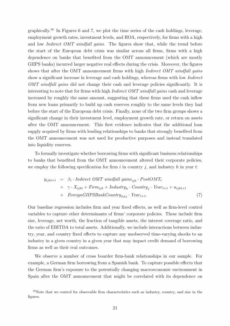
graphically.16 In Figures 6 and 7, we plot the time series of the cash holdings, leverage,

employment growth rates, investment levels, and ROA, respectively, for firms with a high

and low Indirect OMT windfall gains. The figures show that, while the trend before

the start of the European debt crisis was similar across all firms, firms with a high

dependence on banks that benefited from the OMT announcement (which are mostly

GIIPS banks) incurred larger negative real e↵ects during the crisis. Moreover, the figures

shows that after the OMT announcement firms with high Indirect OMT windfall gains

show a significant increase in leverage and cash holdings, whereas firms with low Indirect

OMT windfall gains did not change their cash and leverage policies significantly. It is

interesting to note that for firms with high Indirect OMT windfall gains cash and leverage

increased by roughly the same amount, suggesting that these firms used the cash inflow

from new loans primarily to build up cash reserves roughly to the same levels they had

before the start of the European debt crisis. Finally, none of the two firm groups shows a

significant change in their investment level, employment growth rate, or return on assets

after the OMT announcement. This first evidence indicates that the additional loan

supply acquired by firms with lending relationships to banks that strongly benefited from

the OMT announcement was not used for productive purposes and instead translated

into liquidity reserves.

To formally investigate whether borrowing firms with significant business relationships

to banks that benefited from the OMT announcement altered their corporate policies,

we employ the following specification for firm i in country j, and industry h in year t:

yijht+1 = �1 · Indirect OMT windfall gains ijh · PostOMTt

+ � ·Xijht + Firm ijh + Industryh · Country j · Year t+1 + uijht+1

+ ForeignGIIPSBankCountryk 6=j · Year t+1. (7)

Our baseline regression includes firm and year fixed e↵ects, as well as firm-level control

variables to capture other determinants of firms’ corporate policies. These include firm

size, leverage, net worth, the fraction of tangible assets, the interest coverage ratio, and

the ratio of EBITDA to total assets. Additionally, we include interactions between indus-

try, year, and country fixed e↵ects to capture any unobserved time-varying shocks to an

industry in a given country in a given year that may impact credit demand of borrowing

firms as well as their real outcomes.

We observe a number of cross boarder firm-bank relationships in our sample. For

example, a German firm borrowing from a Spanish bank. To capture possible e↵ects that

the German firm’s exposure to the potentially changing macroeconomic environment in

Spain after the OMT announcement that might be correlated with its dependence on

16Note that we control for observable firm characteristics such as industry, country, and size in thefigures.

21

a Spanish bank (e.g., because the German firm has a subsidiary in Spain), we include

foreign GIIPS bank country times year fixed e↵ects. For the example of the German firm

with a Spanish subsidiary, besides the industry-country-year fixed e↵ect, we additionally

include a Spain-year fixed for this firm.

Results are presented in Table 8. The unit of observation is a firm-year. For ease of

exposure, we only report the results for our key variable of interest, the interaction of

Indirect OMT windfall gains with the PostOMT dummy. The results in Table 8 show

distinct patterns for the behavior of financial and real variables after the OMT program

announcement. For the financial variables, we find a significant increase in both cash

and leverage. Note that the di↵erence of the coe�cients for the change in cash and

change in leverage regressions is small and statistically insignificant (see Column (3)).

This result suggests that both leverage and cash holdings increased by a similar amount,

implying that firms used the liquidity inflow primarily to increase their cash reserves.

More precisely, a one standard deviation increase in Indirect OMT windfall gains implies

an increase in cash and leverage of around 1.9pp.

This result is further confirmed by the fact that we do not find any significant e↵ects

for the real variables. Neither employment nor investment or ROA change significantly for

firms with high Indirect OMT windfall gains in the period after the OMT announcement.

Hence, the primary objective of these firms seems to be to regain financial stability, i.e.,

to increase their cash reserves and reach the pre-crisis cash level again.

Recall, that Panel B of Table 3 reports that primarily low-quality firms benefited

from the expansion in loan volume induced by the increase in value of the sovereign

debt holdings in the period following the OMT program announcement. We now provide

evidence on the relation between real e↵ects and the Indirect OMT windfall gains of

these firms. Panel B of Table 8 presents the results for our baseline regressions for the

five di↵erent corporate policies of firms (i.e., change in cash, change in debt, employment

growth, investment, and return on assets), split based on the firms’ quality. Again, we

classify firms based on their average interest coverage ratio during the sovereign debt

crisis (2009 to 2011).

The general picture that emerges from the table is that the financial e↵ects reported

in Panel B of Table 8 for our entire sample of firms is driven mostly by the low interest

coverage subgroup of firms, while neither high- nor low-quality firms show a significant

relation between Indirect OMT windfall gains of their banks and real economic activity

like employment and investment.

In contrast, Panels C and D of Table 8 documents that zombie firms do not use the

entire funds from their new bank loans to build up cash reserves. For these firms, leverage

increases significantly more than cash holdings. A potential explanation could be that

firms need the proceeds from newly received loans to service interest rate payments on

their existing loans. Note, that this is consistent with the observation, that zombie firms

22

only have an interest coverage ratio of 0.39-0.40, implying that they are unable to service

interest payments from earnings. The Financial Times wrote on this topic that ”The

concern is that these companies - which spend so much of their cash servicing interest

payments that they are unable to invest in new equipment or future growth areas - could

be at least partly to blame for the weak recovery in Europe, hogging resources that could

go to more productive areas”.17. This is also consistent with the fact that for these firms

there are no significant e↵ects on either employment or investment.18 These firms thus

show the typical behavior of zombie firms (Giannetti and Simonov (2013)). Moreover the

quote suggests that the presence of zombie firms might have contagious spillover e↵ects

on healthy firms, which are cut o↵ from lending as loans go to zombie firms instead. Thus,

the next section will investigate whether the presence of zombie firms leads to distortions

for healthy firms operating in the same industry as the zombie firms.

4.4 Zombie Distortions

In a final step, we investigate whether the rising fraction of zombie firms had negative

e↵ects on healthy (non-zombie) firms competing in the same industries. There are two

potential channels through which non-zombie firms that operate in the same industries

as zombie firms could be negatively a↵ected by the prevalence of zombies. First, banks

with incentives to evergreen outstanding loans might shift their loan supply to existing

borrowers that struggle to service their debt. This might lead to a reduction in loan

supply for productive creditworthy firms operating in the same industries, which makes

these firms potentially more financially constrained than firms in industries without such

loan supply distortions. Second, the prevalence of zombie firms might lead to distorted

market competition, which also negatively a↵ects non-zombie firms competing in the same

industries. The normal competitive outcome would be that impaired firms shed workers

and lose market share. However, subsidized loans extended by still undercapitalized banks

kept distressed borrowers artificially alive, which congests the respective markets. The

resulting distorting e↵ects on healthy firms competing in the same industries include, for

example, depressing product market prices and raising market wages by hanging on to the

workers whose productivity at the current firms declined. Due to these two channels, we

expect that a high prevalence of congesting zombie firms in a particular industry resulted

in larger distortions for healthy firms and thus a less vigorous recovery in this industry

compared to industries with a low fraction of zombie firms (see also Caballero, Hoshi,

and Kashyap (2008)).

17Financial Times: Companies: The Rise of the Zombie, January 8th, 201318All results are depicted graphically in Figures 8 and 9, where we plot the time series of the asset-

weighted cash holdings, leverage, employment growth rates, investment levels, and ROA respectively, forhigh quality firms, low quality non-zombie firms, as well as zombie firms, respectively. Note, that weonly consider firms with a high dependence on banks that benefited from the OMT announcement.

23

The basic regression we will run in this section follows Caballero, Hoshi, and Kashyap

(2008) and is given by:

yijht+1 = �1 · Non-Zombie ijht + �2 · Non-Zombie ijht · Fraction Zombiesjht

+ �3 · Non-Zombie ijht · Fraction Zombiesjht · High IC Firm ijht

+ � ·Xijht + Firm ijh + Industryh · Country j · Year t+1 + uijht+1, (8)

where Fraction Zombiesjht measures the fraction of zombies in industry h in country j

at time t.19

We will focus our analysis on real outcomes at the firm level, that is, the dependent

variables are the interest rate paid, employment growth, investment, and productivity.

In particular, if the prevalence of zombies firms in a particular industry is very high, it

is very likely that many banks that act as capital supplier to this industry shifted their

attention to zombie firms. Hence, we expect that non-zombie firms active in this industry

have to pay higher interest rates to still be able to access bank financing. Moreover, due to

the resulting financial constraints and the distorted market competition, firms competing

in industries with a high prevalence of zombie firms should have a lower employment

growth and lower investments compared to firms in industries with only a few zombie

firms. Finally, high-quality non-zombie firms operating in high fraction zombie industries

should have had a higher average productivity. As argued by Caballero, Hoshi, and

Kashyap (2008), due to the competition distortions, these firms had to cut back their

business more strongly in terms of projects and investments. Since firms primarily reduce

investments in projects with a low productivity, the average productivity of their projects

should have increased.

Therefore, our coe�cients of interest are �2 and �3, that is, whether non-zombie

firms, and especially high-quality non-zombie firms, pay higher interest rates, invest less,

have lower employment growth, or a higher average productivity due to the presence

of zombie firms in their industry. In our preferred specification, we include again firm,

and industry-country-year fixed e↵ects. The latter alleviate concerns that the fraction

of zombie firms in the industry in a given a country and year is a proxy for the overall

(un)attractiveness of operating in the industry (for that year). Note, however, that even

without industry-country-year fixed e↵ects, non-zombie firms would have to be more

a↵ected by a industry-specific macroeconomic downturn than zombie firms in order to

get a significant e↵ect of being a non-zombie on interest rates, investment, employment,

or productivity.

Results for this specification are presented in Table 9. The results of the regression

19We use the universe of very large Amadeus firms to calculate the industry fraction of zombie firms.This implies that we have to drop the criterion regarding the syndicate composition for our zombiedefinition.

24

analysis in the table show that low-quality non-zombie firms that operate in industries

with a high zombie fraction do not pay higher interest rates, invest less, or have lower

employment growth rates (�2 is insignificant throughout all specifications). High-quality

non-zombie firms, however, pay higher interest rates, invest significantly less, and also

have significantly lower employment growth rates if they operate in industries with many

zombie firms (�3 is significant throughout all specifications) compared to firms in indus-

tries with a low prevalence of zombie firms. This is consistent with our predictions and

with our previous results, which show that mostly low-quality borrowers benefited from

the loan supply increase. While also non-zombie low-quality firms received additional

loans, these firms mostly used the proceeds to build up cash reserves. If regaining fi-

nancial stability was indeed their primary objective, it seems plausible that these firms

would not have used the loan proceeds to invest or hire people if there were less zom-

bies in their industry. High-quality firms, however, which did not benefit from the loan

supply increase (instead they even had to pay higher interest rates), su↵er from the pres-

ence of zombie firms in their industry. For these firms, investment levels are significantly

depressed if they operate in industries with a significant fraction of zombie firms. On

average, the fraction of zombie firms increased by 8.9% after OMT. Considering the es-

timates in Columns (2) and (4), this implies that high-quality non-zombie firms invest

between 11.6% and 13.3% of capital less compared to a scenario where the fraction of

zombies had stayed at its pre-OMT level. An industry at the 95th percentile saw an

increase of zombie firms of 30%, implying that high-quality non-zombie firms invested

between 39% and 44% of capital less due to the increase in the fraction of zombie firms.

When looking at employment growth, we find that firms that saw an increase of 8.9% in

the fraction of zombie firms in their industry had 3.6% to 4.4% lower employment growth

rates. Considering again the 90th percentile, we find that high-quality non-zombie firms

in this industry had 12% to 15% lower employment growth rates.

Finally, to ensure that the negative e↵ects on healthy firms that are active in industries

with a high zombie firm prevalence was indeed caused by distorted market competition, we

analyze whether these negative e↵ects were more intense for healthy firms in competitive

industries. In particular, the prevalence of zombie firms should not strongly a↵ect non-

zombie firms in a non-competitive industry, because these firms are generally not very

a↵ected by the behavior of firms in the same industry. Hence, whether impaired firms

downsized their business or whether zombie lending kept these firms afloat and thereby

prevented an adjustment process should not have significantly a↵ected the behavior and

performance of healthy firms when these firms were active in a non-competitive industry.

Table 10 presents the results for this test. First, the results show that, due to a

loan supply shift to zombie firms, all high-quality non-zombie firms had to pay higher

interest rates if the prevalence of zombie firms in their industry was particularly high,

irrespective of whether the industry is competitive or not. However, only high-quality

25

non-zombie firms that operate in competitive industries with many zombie firms were

significantly negatively a↵ected (i.e, lower investments and employment growth), while

high-quality non-zombie firms in non-competitive industries did not su↵er real e↵ects due

to the presence of zombie firms in their industries. Again low-quality non-zombie firms

are not negatively a↵ected by the presence of zombie firms in their industries, irrespective

of whether the industry is competitive or not. These results suggest that indeed high-

quality firms su↵er real e↵ects caused by distortions of competitive forces that are due

to zombie lending to their industries.

5 Conclusion

In this paper, we show that the announcement of the OMT program has significantly

improved the health of banks in the periphery of Europe. By substantially reducing

the yields on periphery sovereign debt, GIIPS banks could realize significant windfall

gains on their large sovereign debt holdings. These gains significantly reduced bank risk

and allowed banks to access market based financing again. The increase in bank health

translated into an increased loan supply to the corporate sector, especially to low-quality

borrowers. We show that this increase in loan supply to low-quality borrowers is at

least partly driven by zombie lending motives of high gain banks that remain weakly-

capitalized after the OMT announcement. The analysis thus highlights the importance of

recapitalizing banks adequately to prevent them from engaging in zombie lending. Non-

zombie firms that regain access to bank based financing use the cash inflow from new

bank loans to build up cash reserves. Zombie firms, on the other hand, are not able to

use the inflow from new bank loans to build up cash reserves one for one. Neither group

of firms show a significant increase in real activity, that is, an increase in employment or

investment.

Moreover, we find that high-quality non-zombie firms, i.e., firms that did not benefit

from the increase in bank loan supply are negatively a↵ected if they operate in industries

with a higher fraction of zombie firms. Both their employment growth and investment

are depressed by the increased fraction of zombie firms in their industry.

More broadly, our paper shows that central banks can conduct backdoor recapitaliza-

tions of the banking sector, if they are able to influence the prices of assets that banks

hold in relatively large quantities. By increasing the value of these assets banks can

realize significant gains which improves their equity positions. However, central banks

need to pay close attention to the magnitude of the gain realized by undercapitalized

banks. If the gains are too low to adequately recapitalize (some) banks, zombie lending

incentives might arise. This can lead to significant distortions in the respective industries,

as high-quality firms operating in industries with a high fraction of zombies su↵er from

significantly depressed employment growth rates and investment.

26

References

Acharya, V. V., T. Eisert, C. Eufinger, and C. W. Hirsch (2015): “Real

e↵ects of the sovereign debt crisis in Europe: Evidence from syndicated loans,” CEPR

Discussion Paper No. DP10108.

Acharya, V. V., B. Imbierowicz, S. Steffen, and D. Teichmann (2015): “Does

the Lack of Financial Stability Impair the Transmission of Monetary Policy?,” Working

Paper.

Acharya, V. V., D. Pierret, and S. Steffen (2015): “Lender of Last Resort versus

Buyer of Last Resort - Evidence from the European Sovereign Debt Crisis,” Working

Paper.

Acharya, V. V., and S. Steffen (2013): “Falling Short of Expectations? Stress-

Testing the European Banking System,” Working Paper.

(2014): “The Greatest Carry Trade Ever? Understanding Eurozone Bank

Risks,” Journal of Financial Economics, 115(2), 215–236.

Agarwal, S., S. Chomsisengphet, N. Mahoney, and J. Stroebel (2015): “Do

Banks Pass Through Credit Expansions to Consumers Who Want To Borrow?,”

Working Paper.

Altavilla, C., D. Giannone, and M. Lenza (2014): “The Financial and Macroeco-

nomic e↵ects of OMT Announcements,” ECB Working Paper.

Caballero, R. J., T. Hoshi, and A. K. Kashyap (2008): “Zombie Lending and

Depressed Restructuring in Japan,” The American Economic Review, pp. 1943–1977.

Chodorow-Reich, G. (2014): “The Employment E↵ects of Credit Market Disrup-

tions: Firm-level Evidence from the 2008-09 Financial Crisis,” Quarterly Journal of

Economics, 129, 1–59.

Diamond, D., and R. Rajan (2000): “A Theory of Bank Capital,” Journal of Finance,

55(6), 2431–2465.

Diamond, D. W. (1991): “Monitoring and reputation: The choice between bank loans

and directly placed debt,” Journal of Political Economy, 99(4), 689–721.

Ferrando, A., A. A. Popov, and G. F. Udell (2015): “Sovereign Stress, Uncon-

ventional Monetary Policy, and SME Access to Fina nce,” Working Paper.

Giannetti, M., and A. Simonov (2013): “On the Real E↵ects of Bank Bailouts: Micro

Evidence from Japan,” American Economic Journal: Macroeconomics, 5(1), 135–67.

27

Haldane, A. (2012): “The Dog and the Frisbee,” Bank of England Speech.

Kane, E. J. (1989): The S & L insurance mess: how did it happen? The Urban Insitute.

Khwaja, A. I., and A. Mian (2008): “Tracing the Impact of Bank Liquidity Shocks:

Evidence from an Emerging Market,” American Economic Review, 98(4), 1413–1442.

Krishnamurthy, A., S. Nagel, and A. Vissing-Jorgensen (2014): “ECB policies

involving government bond purchases: Impact and channels,” Working Paper.

Krishnamurthy, A., and A. Vissing-Jorgensen (2011): “The E↵ects of Quantita-

tive Easing on Interest Rates: Channels and Implications for Policy,” Brookings Papers

on Economics Activity.

Peek, J., and E. S. Rosengreen (2005): “Unnatural Selection: Perverse Incentives

and the Allocation of Credit in Japan,” American Economic Review, 95(4), 1144–1166.

Peek, J., and E. S. Rosengren (2005): “Unnatural Selection: Perverse Incentives and

the Misallocation of Credit in Japan,” American Economic Review, 95(4), 1144–1166.

Saka, O., A.-M. Fuertes, and E. Kalotychou (2015): “ECB policy and Eurozone

fragility: Was De Grauwe right?,” Journal of International Money and Finance, 54,

168–185.

Saunders, A., and S. Steffen (2011): “The costs of being private: Evidence from

the loan market,” Review of Financial Studies, 24(12), 4091–4122.

Standard&Poor’s (2010): A Guide To The European Loan Market. New York, NY:

The McGraw-Hill Companies, Inc.

Sufi, A. (2007): “Information asymmetry and financing arrangements: Evidence from

syndicated loans,” Journal of Finance, 62(2), 629–668.

Szczerbowicz, U., et al. (2012): “The ECB unconventional monetary policies: have

they lowered market borrowing costs for banks and governments?,” Working Paper.

28

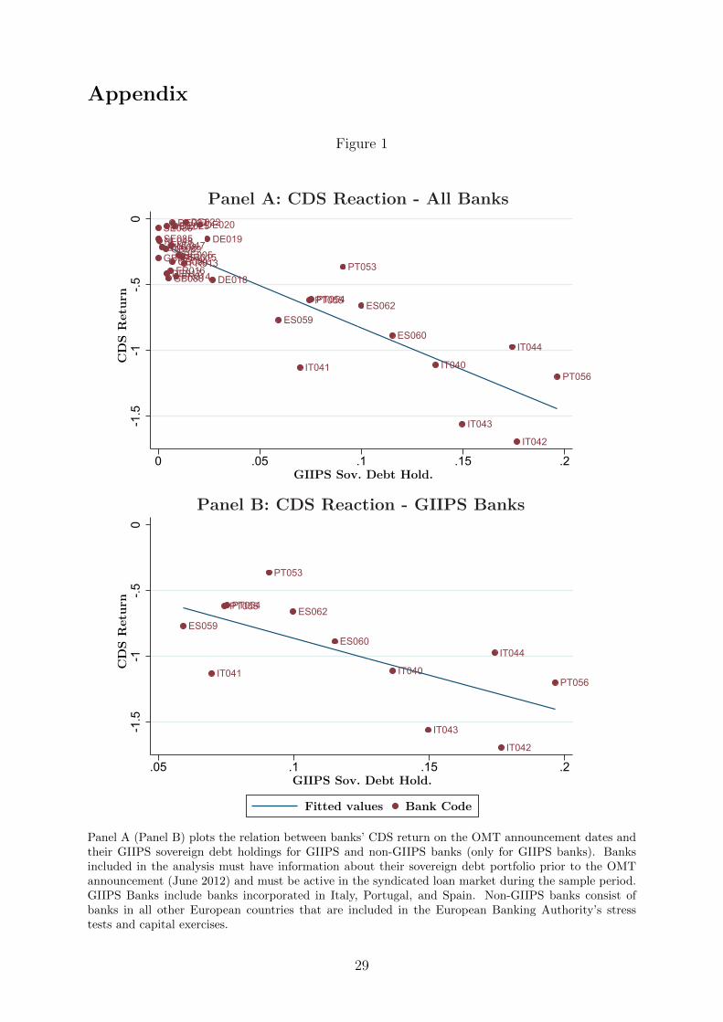
Appendix

Figure 1

IT042

PT056

ES060

PT054PT055

IT043

ES059

PT053

IT040

ES062

IT041

IT044

-1.5

-1-.5

0C

DS

Ret

urn

.05 .1 .15 .2GIIPS Sov. Debt Hold.

Fitted values Bank Code

Panel B: CDS Reaction - GIIPS Banks

FR013FR015

IT042

PT056

ES060

PT054PT055

IT043

ES059

GB090

DE021

PT053DE018FR014

DE020

DK008

DE017

GB089

DE025

NL047

IT040

BE005

ES062

DE019

DE027

GB091

DE022

NL048

GB088

SE085

FR016

SE086

IT041

IT044

-1.5

-1-.5

0C

DS

Ret

urn

0 .05 .1 .15 .2GIIPS Sov. Debt Hold.

Panel A: CDS Reaction - All Banks

Panel A (Panel B) plots the relation between banks’ CDS return on the OMT announcement dates andtheir GIIPS sovereign debt holdings for GIIPS and non-GIIPS banks (only for GIIPS banks). Banksincluded in the analysis must have information about their sovereign debt portfolio prior to the OMTannouncement (June 2012) and must be active in the syndicated loan market during the sample period.GIIPS Banks include banks incorporated in Italy, Portugal, and Spain. Non-GIIPS banks consist ofbanks in all other European countries that are included in the European Banking Authority’s stresstests and capital exercises.

29

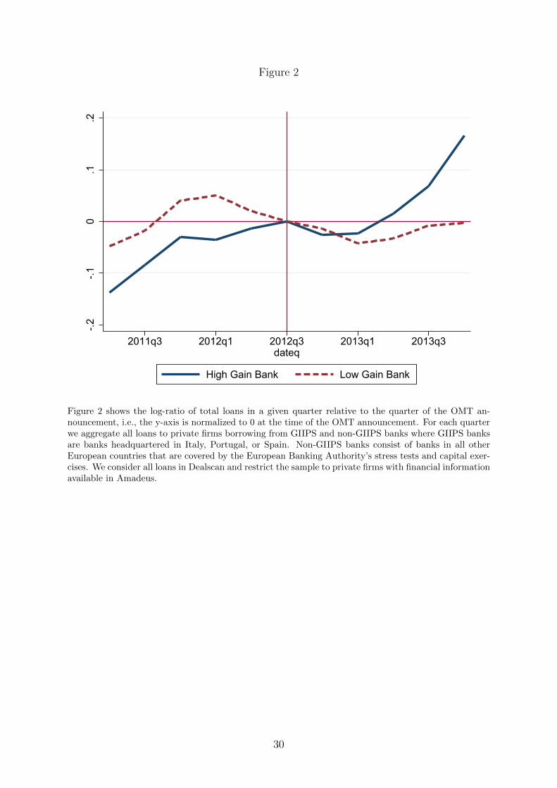
Figure 2

-.2

-.1

0.1

.2

2011q3 2012q1 2012q3 2013q1 2013q3

dateq

High Gain Bank Low Gain Bank

Figure 2 shows the log-ratio of total loans in a given quarter relative to the quarter of the OMT an-nouncement, i.e., the y-axis is normalized to 0 at the time of the OMT announcement. For each quarterwe aggregate all loans to private firms borrowing from GIIPS and non-GIIPS banks where GIIPS banksare banks headquartered in Italy, Portugal, or Spain. Non-GIIPS banks consist of banks in all otherEuropean countries that are covered by the European Banking Authority’s stress tests and capital exer-cises. We consider all loans in Dealscan and restrict the sample to private firms with financial informationavailable in Amadeus.

30

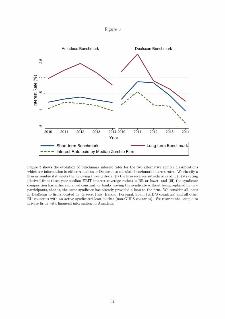
Figure 3

.51

1.5

22.

5

2010 2011 2012 2013 2014 2010 2011 2012 2013 2014

Amadeus Benchmark Dealscan Benchmark

Short-term Benchmark Long-term BenchmarkInterest Rate paid by Median Zombie Firm

Inte

rest

Rat

e (%

)

Year

Figure 3 shows the evolution of benchmark interest rates for the two alternative zombie classificationswhich use information in either Amadeus or Dealscan to calculate benchmark interest rates. We classify afirm as zombie if it meets the following three criteria: (i) the firm receives subsidized credit, (ii) its rating(derived from three year median EBIT interest coverage ratios) is BB or lower, and (iii) the syndicatecomposition has either remained constant, or banks leaving the syndicate without being replaced by newparticipants, that is, the same syndicate has already provided a loan to the firm. We consider all loansin DealScan to firms located in: Greece, Italy, Ireland, Portugal, Spain (GIIPS countries) and all otherEU countries with an active syndicated loan market (non-GIIPS countries). We restrict the sample toprivate firms with financial information in Amadeus.

31

Figure 4

.04

.06

.08

.1.1

2A

sset

-wei

ghte

d zo

mbi

e fra

ctio

n

2010 2011 2012 2013 2014Year

Benchmark Dealscan Benchmark Amadeus

Figure 4 shows the evolution of the asset-weighted fraction of zombies in our sample for the two alternativezombie classifications which use information in either Amadeus or Dealscan to calculate benchmarkinterest rates. We classify a firm as zombie if it meets the following three criteria: (i) the firm receivessubsidized credit, (ii) its rating (derived from three year median EBIT interest coverage ratios) is BB orlower, and (iii) the syndicate composition has either remained constant, or banks leaving the syndicatewithout being replaced by new participants, that is, the same syndicate has already provided a loanto the firm. We consider all loans in DealScan to firms located in: Greece, Italy, Ireland, Portugal,Spain (GIIPS countries) and all other EU countries with an active syndicated loan market (non-GIIPScountries). We restrict the sample to private firms with financial information in Amadeus.

32

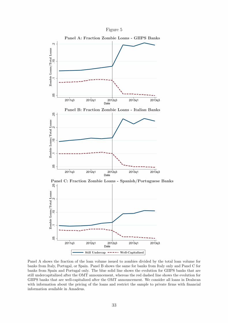
Figure 5

.05

.1.15

.2Zo

mbi

e Lo

ans/

Tot

al L

oans

2011q3 2012q1 2012q3 2013q1 2013q3Date

Panel A: Fraction Zombie Loans - GIIPS Banks

.05

.1.15

.2.25

Zom

bie

Loan

s/T

otal

Loa

ns

2011q3 2012q1 2012q3 2013q1 2013q3Date

Panel B: Fraction Zombie Loans - Italian Banks

.05

.1.15

.2.25

Zom

bie

Loan

s/T

otal

Loa

ns

2011q3 2012q1 2012q3 2013q1 2013q3Date

Still Undercap Well-Capitalized

Panel C: Fraction Zombie Loans - Spanish/Portuguese Banks

Panel A shows the fraction of the loan volume issued to zombies divided by the total loan volume forbanks from Italy, Portugal, or Spain. Panel B shows the same for banks from Italy only and Panel C forbanks from Spain and Portugal only. The blue solid line shows the evolution for GIIPS banks that arestill undercapitalized after the OMT announcement, whereas the red dashed line shows the evolution forGIIPS banks that are well-capitalized after the OMT announcement. We consider all loans in Dealscanwith information about the pricing of the loans and restrict the sample to private firms with financialinformation available in Amadeus.

33

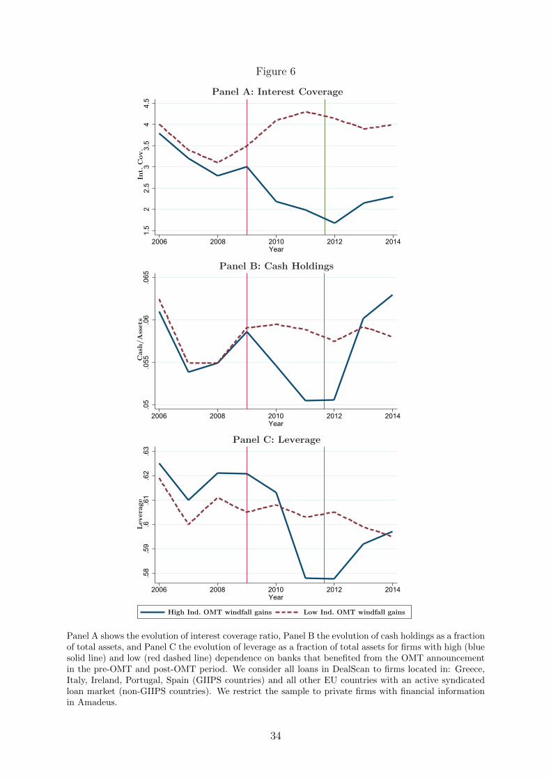
Figure 6

.58

.59

.6.61

.62

.63

Leve

rage

2006 2008 2010 2012 2014Year

High Ind. OMT windfall gains Low Ind. OMT windfall gains

Panel C: Leverage

.05

.055

.06

.065

Cas

h/A

sset

s

2006 2008 2010 2012 2014Year

Panel B: Cash Holdings

1.5

22.5

33.5

44.5

Int.

Cov

.

2006 2008 2010 2012 2014Year

Panel A: Interest Coverage

Panel A shows the evolution of interest coverage ratio, Panel B the evolution of cash holdings as a fractionof total assets, and Panel C the evolution of leverage as a fraction of total assets for firms with high (bluesolid line) and low (red dashed line) dependence on banks that benefited from the OMT announcementin the pre-OMT and post-OMT period. We consider all loans in DealScan to firms located in: Greece,Italy, Ireland, Portugal, Spain (GIIPS countries) and all other EU countries with an active syndicatedloan market (non-GIIPS countries). We restrict the sample to private firms with financial informationin Amadeus.

34

Figure 7

-.02

0.02

.04

.06

Em

p G

row

th

2006 2008 2010 2012 2014Year

Panel A: Employment Growth

.1.12

.14

.16

.18

.2C

AP

X

2006 2008 2010 2012 2014Year

Panel B: Investment

22.5

33.5

44.5

55.5

RO

A

2006 2008 2010 2012 2014Year

Panel C: Return on Assets

High Ind. OMT windfall gains Low Ind. OMT windfall gains

Panel A shows the evolution of employment growth rates, Panel B the evolution of capital expendituresas a fraction of tangible assets, and Panel C the evolution of the return on assets for firms with high (bluesolid line) and low (red dashed line) dependence on banks that benefited from the OMT announcementin the pre-OMT and post-OMT period. We consider all loans in DealScan to firms located in: Greece,Italy, Ireland, Portugal, Spain (GIIPS countries) and all other EU countries with an active syndicatedloan market (non-GIIPS countries). We restrict the sample to private firms with financial informationin Amadeus.

35

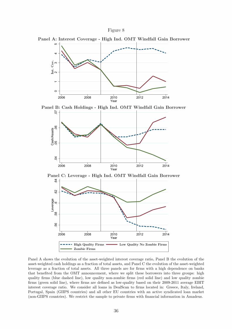
Figure 8

01

23

45

Int.

Cov

.

2006 2008 2010 2012 2014Year

Panel A: Interest Coverage - High Ind. OMT Windfall Gain Borrower

.04

.05

.06

.07

Cash/Assets

2006 2008 2010 2012 2014Year

Panel B: Cash Holdings - High Ind. OMT Windfall Gain Borrower

.56

.58

.6.62

.64

Leverage

2006 2008 2010 2012 2014Year

High Quality Firms Low Quality No Zombie FirmsZombie Firms

Panel C: Leverage - High Ind. OMT Windfall Gain Borrower

Panel A shows the evolution of the asset-weighted interest coverage ratio, Panel B the evolution of theasset-weighted cash holdings as a fraction of total assets, and Panel C the evolution of the asset-weightedleverage as a fraction of total assets. All three panels are for firms with a high dependence on banksthat benefited from the OMT announcement, where we split these borrowers into three groups: highquality firms (blue dashed line), low quality non-zombie firms (red solid line) and low quality zombiefirms (green solid line), where firms are defined as low-quality based on their 2009-2011 average EBITinterest coverage ratio. We consider all loans in DealScan to firms located in: Greece, Italy, Ireland,Portugal, Spain (GIIPS countries) and all other EU countries with an active syndicated loan market(non-GIIPS countries). We restrict the sample to private firms with financial information in Amadeus.

36

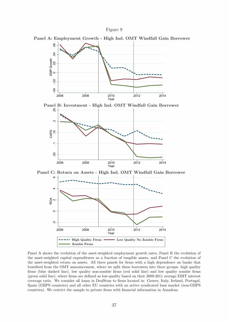
Figure 9

-.0

4-.

02

0.0

2.0

4.0

6

EM

P G

row

th

2006 2008 2010 2012 2014

Year

Panel A: Employment Growth - High Ind. OMT Windfall Gain Borrower

.05

.1.1

5.2

.25

CA

PX

2006 2008 2010 2012 2014

Year

Panel B: Investment - High Ind. OMT Windfall Gain Borrower

-20

24

6

RO

A

2006 2008 2010 2012 2014

Year

Panel C: Return on Assets - High Ind. OMT Windfall Gain Borrower

High Quality Firms Low Quality No Zombie FirmsZombie Firms

Panel A shows the evolution of the asset-weighted employment growth rates, Panel B the evolution ofthe asset-weighted capital expenditures as a fraction of tangible assets, and Panel C the evolution ofthe asset-weighted return on assets. All three panels for firms with a high dependence on banks thatbenefited from the OMT announcement, where we split these borrowers into three groups: high qualityfirms (blue dashed line), low quality non-zombie firms (red solid line) and low quality zombie firms(green solid line), where firms are defined as low-quality based on their 2009-2011 average EBIT interestcoverage ratio. We consider all loans in DealScan to firms located in: Greece, Italy, Ireland, Portugal,Spain (GIIPS countries) and all other EU countries with an active syndicated loan market (non-GIIPScountries). We restrict the sample to private firms with financial information in Amadeus.

37

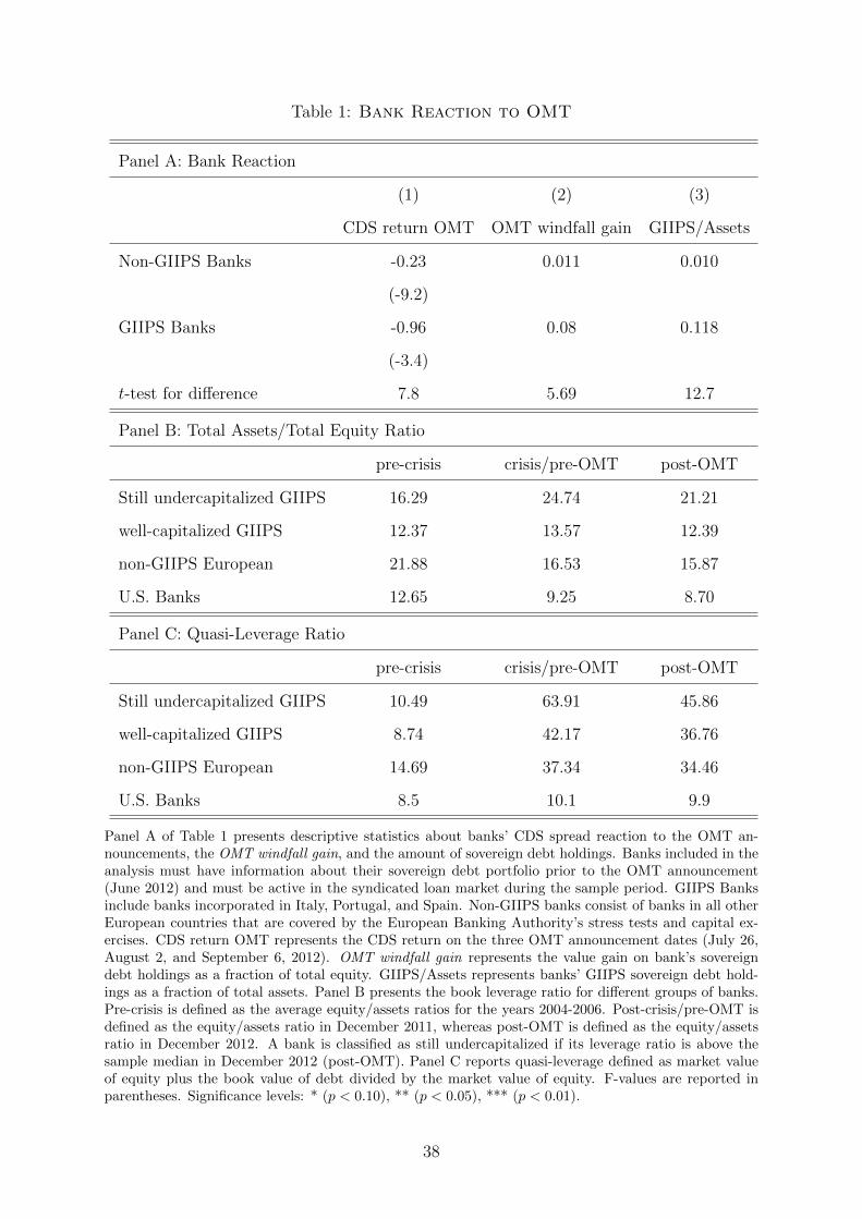
Table 1: Bank Reaction to OMT

Panel A: Bank Reaction

(1) (2) (3)

CDS return OMT OMT windfall gain GIIPS/Assets

Non-GIIPS Banks -0.23 0.011 0.010

(-9.2)

GIIPS Banks -0.96 0.08 0.118

(-3.4)

t-test for di↵erence 7.8 5.69 12.7

Panel B: Total Assets/Total Equity Ratio

pre-crisis crisis/pre-OMT post-OMT

Still undercapitalized GIIPS 16.29 24.74 21.21

well-capitalized GIIPS 12.37 13.57 12.39

non-GIIPS European 21.88 16.53 15.87

U.S. Banks 12.65 9.25 8.70

Panel C: Quasi-Leverage Ratio

pre-crisis crisis/pre-OMT post-OMT

Still undercapitalized GIIPS 10.49 63.91 45.86

well-capitalized GIIPS 8.74 42.17 36.76

non-GIIPS European 14.69 37.34 34.46

U.S. Banks 8.5 10.1 9.9

Panel A of Table 1 presents descriptive statistics about banks’ CDS spread reaction to the OMT an-nouncements, the OMT windfall gain, and the amount of sovereign debt holdings. Banks included in theanalysis must have information about their sovereign debt portfolio prior to the OMT announcement(June 2012) and must be active in the syndicated loan market during the sample period. GIIPS Banksinclude banks incorporated in Italy, Portugal, and Spain. Non-GIIPS banks consist of banks in all otherEuropean countries that are covered by the European Banking Authority’s stress tests and capital ex-ercises. CDS return OMT represents the CDS return on the three OMT announcement dates (July 26,August 2, and September 6, 2012). OMT windfall gain represents the value gain on bank’s sovereigndebt holdings as a fraction of total equity. GIIPS/Assets represents banks’ GIIPS sovereign debt hold-ings as a fraction of total assets. Panel B presents the book leverage ratio for di↵erent groups of banks.Pre-crisis is defined as the average equity/assets ratios for the years 2004-2006. Post-crisis/pre-OMT isdefined as the equity/assets ratio in December 2011, whereas post-OMT is defined as the equity/assetsratio in December 2012. A bank is classified as still undercapitalized if its leverage ratio is above thesample median in December 2012 (post-OMT). Panel C reports quasi-leverage defined as market valueof equity plus the book value of debt divided by the market value of equity. F-values are reported inparentheses. Significance levels: * (p < 0.10), ** (p < 0.05), *** (p < 0.01).

38

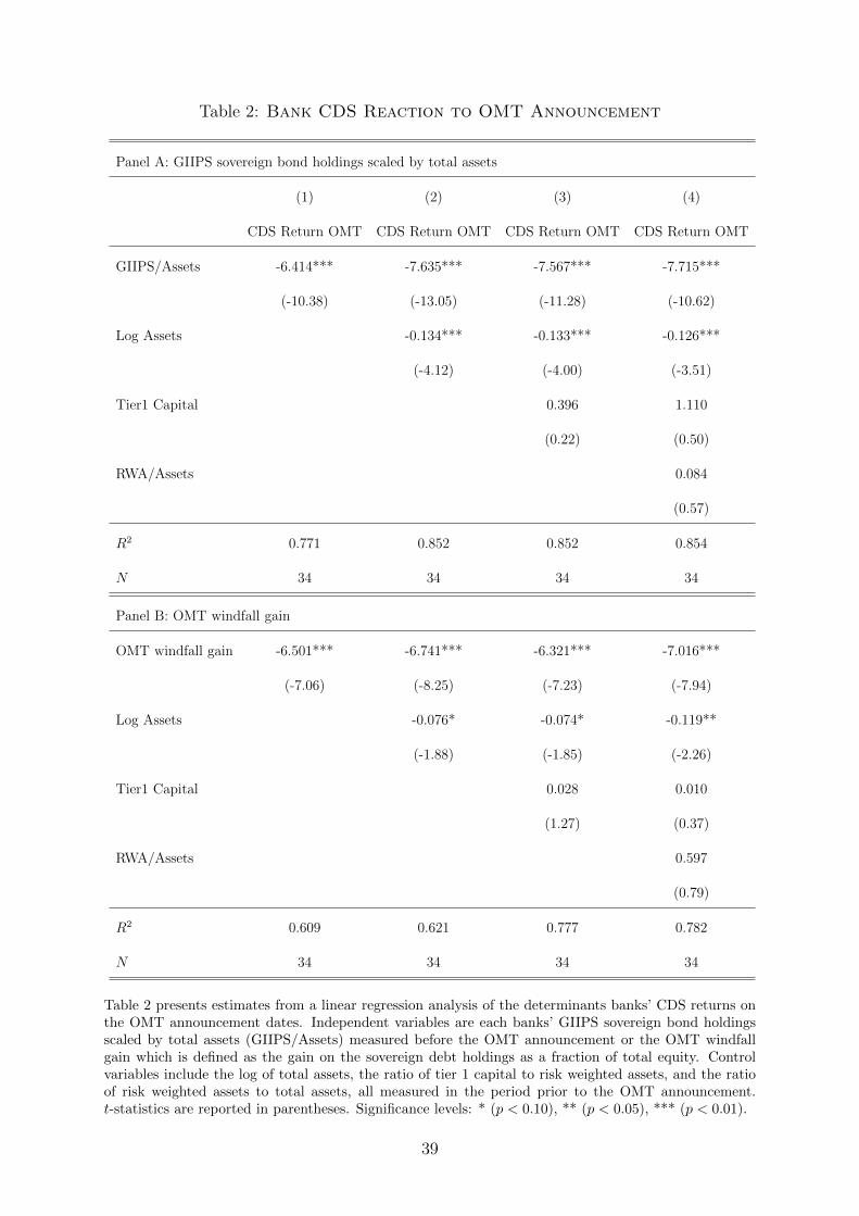
Table 2: Bank CDS Reaction to OMT Announcement

Panel A: GIIPS sovereign bond holdings scaled by total assets

(1) (2) (3) (4)

CDS Return OMT CDS Return OMT CDS Return OMT CDS Return OMT

GIIPS/Assets -6.414*** -7.635*** -7.567*** -7.715***

(-10.38) (-13.05) (-11.28) (-10.62)

Log Assets -0.134*** -0.133*** -0.126***

(-4.12) (-4.00) (-3.51)

Tier1 Capital 0.396 1.110

(0.22) (0.50)

RWA/Assets 0.084

(0.57)

R2 0.771 0.852 0.852 0.854

N 34 34 34 34

Panel B: OMT windfall gain

OMT windfall gain -6.501*** -6.741*** -6.321*** -7.016***

(-7.06) (-8.25) (-7.23) (-7.94)

Log Assets -0.076* -0.074* -0.119**

(-1.88) (-1.85) (-2.26)

Tier1 Capital 0.028 0.010

(1.27) (0.37)

RWA/Assets 0.597

(0.79)

R2 0.609 0.621 0.777 0.782

N 34 34 34 34

Table 2 presents estimates from a linear regression analysis of the determinants banks’ CDS returns onthe OMT announcement dates. Independent variables are each banks’ GIIPS sovereign bond holdingsscaled by total assets (GIIPS/Assets) measured before the OMT announcement or the OMT windfallgain which is defined as the gain on the sovereign debt holdings as a fraction of total equity. Controlvariables include the log of total assets, the ratio of tier 1 capital to risk weighted assets, and the ratioof risk weighted assets to total assets, all measured in the period prior to the OMT announcement.t-statistics are reported in parentheses. Significance levels: * (p < 0.10), ** (p < 0.05), *** (p < 0.01).

39

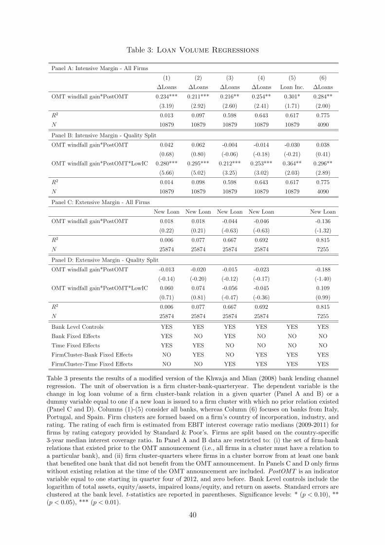
Table 3: Loan Volume Regressions

Panel A: Intensive Margin - All Firms

(1) (2) (3) (4) (5) (6)

�Loans �Loans �Loans �Loans Loan Inc. �Loans

OMT windfall gain*PostOMT 0.234*** 0.211*** 0.216** 0.254** 0.301* 0.284**

(3.19) (2.92) (2.60) (2.41) (1.71) (2.00)

R2 0.013 0.097 0.598 0.643 0.617 0.775

N 10879 10879 10879 10879 10879 4090

Panel B: Intensive Margin - Quality Split

OMT windfall gain*PostOMT 0.042 0.062 -0.004 -0.014 -0.030 0.038

(0.68) (0.80) (-0.06) (-0.18) (-0.21) (0.41)

OMT windfall gain*PostOMT*LowIC 0.280*** 0.295*** 0.212*** 0.253*** 0.364** 0.296**

(5.66) (5.02) (3.25) (3.02) (2.03) (2.89)

R2 0.014 0.098 0.598 0.643 0.617 0.775

N 10879 10879 10879 10879 10879 4090

Panel C: Extensive Margin - All Firms

New Loan New Loan New Loan New Loan New Loan

OMT windfall gain*PostOMT 0.018 0.018 -0.044 -0.046 -0.136

(0.22) (0.21) (-0.63) (-0.63) (-1.32)

R2 0.006 0.077 0.667 0.692 0.815

N 25874 25874 25874 25874 7255

Panel D: Extensive Margin - Quality Split

OMT windfall gain*PostOMT -0.013 -0.020 -0.015 -0.023 -0.188

(-0.14) (-0.20) (-0.12) (-0.17) (-1.40)

OMT windfall gain*PostOMT*LowIC 0.060 0.074 -0.056 -0.045 0.109

(0.71) (0.81) (-0.47) (-0.36) (0.99)

R2 0.006 0.077 0.667 0.692 0.815

N 25874 25874 25874 25874 7255

Bank Level Controls YES YES YES YES YES YES

Bank Fixed E↵ects YES NO YES NO NO NO

Time Fixed E↵ects YES YES NO NO NO NO

FirmCluster-Bank Fixed E↵ects NO YES NO YES YES YES

FirmCluster-Time Fixed E↵ects NO NO YES YES YES YES

Table 3 presents the results of a modified version of the Khwaja and Mian (2008) bank lending channelregression. The unit of observation is a firm cluster-bank-quarteryear. The dependent variable is thechange in log loan volume of a firm cluster-bank relation in a given quarter (Panel A and B) or adummy variable equal to one if a new loan is issued to a firm cluster with which no prior relation existed(Panel C and D). Columns (1)-(5) consider all banks, whereas Column (6) focuses on banks from Italy,Portugal, and Spain. Firm clusters are formed based on a firm’s country of incorporation, industry, andrating. The rating of each firm is estimated from EBIT interest coverage ratio medians (2009-2011) forfirms by rating category provided by Standard & Poor’s. Firms are split based on the country-specific3-year median interest coverage ratio. In Panel A and B data are restricted to: (i) the set of firm-bankrelations that existed prior to the OMT announcement (i.e., all firms in a cluster must have a relation toa particular bank), and (ii) firm cluster-quarters where firms in a cluster borrow from at least one bankthat benefited one bank that did not benefit from the OMT announcement. In Panels C and D only firmswithout existing relation at the time of the OMT announcement are included. PostOMT is an indicatorvariable equal to one starting in quarter four of 2012, and zero before. Bank Level controls include thelogarithm of total assets, equity/assets, impaired loans/equity, and return on assets. Standard errors areclustered at the bank level. t-statistics are reported in parentheses. Significance levels: * (p < 0.10), **(p < 0.05), *** (p < 0.01).

40

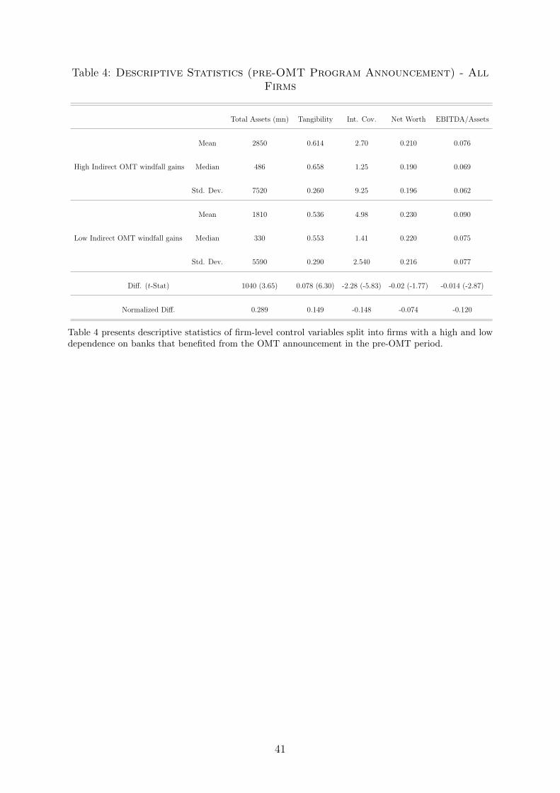
Table 4: Descriptive Statistics (pre-OMT Program Announcement) - AllFirms

Total Assets (mn) Tangibility Int. Cov. Net Worth EBITDA/Assets

Mean 2850 0.614 2.70 0.210 0.076

High Indirect OMT windfall gains Median 486 0.658 1.25 0.190 0.069

Std. Dev. 7520 0.260 9.25 0.196 0.062

Mean 1810 0.536 4.98 0.230 0.090

Low Indirect OMT windfall gains Median 330 0.553 1.41 0.220 0.075

Std. Dev. 5590 0.290 2.540 0.216 0.077

Di↵. (t-Stat) 1040 (3.65) 0.078 (6.30) -2.28 (-5.83) -0.02 (-1.77) -0.014 (-2.87)

Normalized Di↵. 0.289 0.149 -0.148 -0.074 -0.120

Table 4 presents descriptive statistics of firm-level control variables split into firms with a high and lowdependence on banks that benefited from the OMT announcement in the pre-OMT period.

41

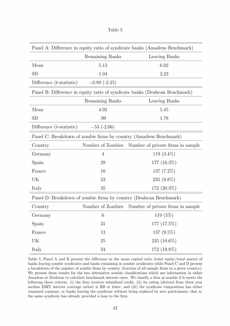
Table 5

Panel A: Di↵erence in equity ratio of syndicate banks (Amadeus Benchmark)

Remaining Banks Leaving Banks

Mean 5.13 6.02

SD 1.04 2.23

Di↵erence (t-statistic) -.0.89 (-2.25)

Panel B: Di↵erence in equity ratio of syndicate banks (Dealscan Benchmark)

Remaining Banks Leaving Banks

Mean 4.92 5.45

SD .99 1.78

Di↵erence (t-statistic) -.53 (-2.06)

Panel C: Breakdown of zombie firms by country (Amadeus Benchmark)

Country Number of Zombies Number of private firms in sample

Germany 4 119 (3.4%)

Spain 29 177 (16.3%)

France 10 137 (7.2%)

UK 23 235 (9.8%)

Italy 35 172 (20.3%)

Panel D: Breakdown of zombie firms by country (Dealscan Benchmark)

Country Number of Zombies Number of private firms in sample

Germany 6 119 (5%)

Spain 31 177 (17.5%)

France 13 137 (9.5%)

UK 25 235 (10.6%)

Italy 34 172 (19.8%)

Table 5, Panel A and B present the di↵erence in the mean capital ratio (total equity/total assets) ofbanks leaving zombie syndicates and banks remaining in zombie syndicates while Panel C and D presenta breakdown of the number of zombie firms by country (fraction of all sample firms in a given country).We present these results for the two alternative zombie classifications which use information in eitherAmadeus or Dealscan to calculate benchmark interest rates. We classify a firm as zombie if it meets thefollowing three criteria: (i) the firm receives subsidized credit, (ii) its rating (derived from three yearmedian EBIT interest coverage ratios) is BB or lower, and (iii) the syndicate composition has eitherremained constant, or banks leaving the syndicate without being replaced by new participants, that is,the same syndicate has already provided a loan to the firm.

42

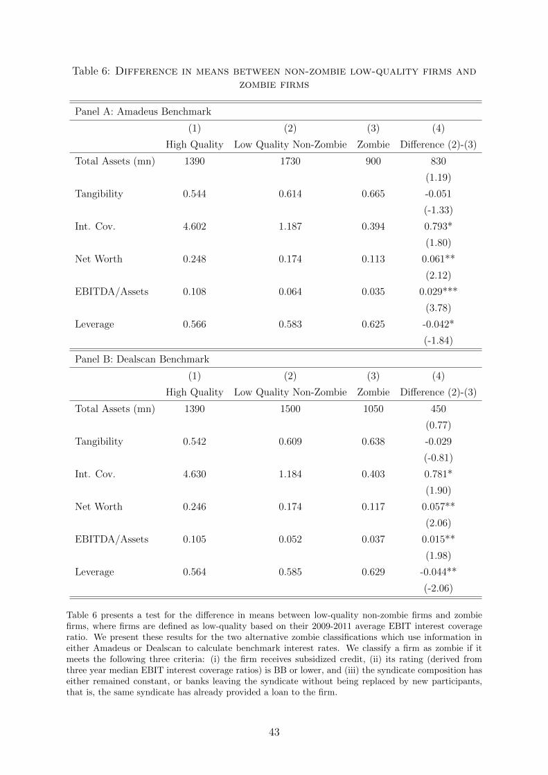
Table 6: Difference in means between non-zombie low-quality firms andzombie firms

Panel A: Amadeus Benchmark

(1) (2) (3) (4)

High Quality Low Quality Non-Zombie Zombie Di↵erence (2)-(3)

Total Assets (mn) 1390 1730 900 830

(1.19)

Tangibility 0.544 0.614 0.665 -0.051

(-1.33)

Int. Cov. 4.602 1.187 0.394 0.793*

(1.80)

Net Worth 0.248 0.174 0.113 0.061**

(2.12)

EBITDA/Assets 0.108 0.064 0.035 0.029***

(3.78)

Leverage 0.566 0.583 0.625 -0.042*

(-1.84)

Panel B: Dealscan Benchmark

(1) (2) (3) (4)

High Quality Low Quality Non-Zombie Zombie Di↵erence (2)-(3)

Total Assets (mn) 1390 1500 1050 450

(0.77)

Tangibility 0.542 0.609 0.638 -0.029

(-0.81)

Int. Cov. 4.630 1.184 0.403 0.781*

(1.90)

Net Worth 0.246 0.174 0.117 0.057**

(2.06)

EBITDA/Assets 0.105 0.052 0.037 0.015**

(1.98)

Leverage 0.564 0.585 0.629 -0.044**

(-2.06)

Table 6 presents a test for the di↵erence in means between low-quality non-zombie firms and zombiefirms, where firms are defined as low-quality based on their 2009-2011 average EBIT interest coverageratio. We present these results for the two alternative zombie classifications which use information ineither Amadeus or Dealscan to calculate benchmark interest rates. We classify a firm as zombie if itmeets the following three criteria: (i) the firm receives subsidized credit, (ii) its rating (derived fromthree year median EBIT interest coverage ratios) is BB or lower, and (iii) the syndicate composition haseither remained constant, or banks leaving the syndicate without being replaced by new participants,that is, the same syndicate has already provided a loan to the firm.

43

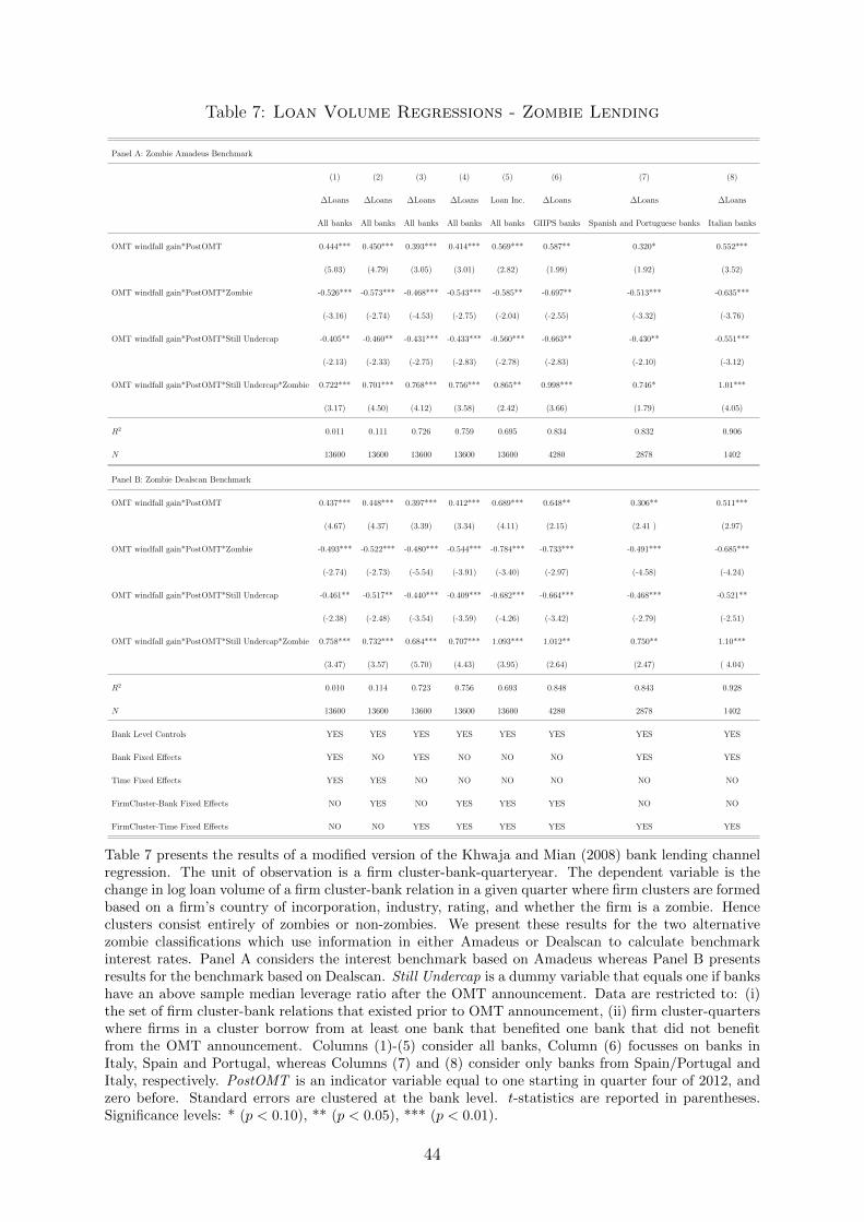
Table 7: Loan Volume Regressions - Zombie Lending

Panel A: Zombie Amadeus Benchmark

(1) (2) (3) (4) (5) (6) (7) (8)

�Loans �Loans �Loans �Loans Loan Inc. �Loans �Loans �Loans

All banks All banks All banks All banks All banks GIIPS banks Spanish and Portuguese banks Italian banks

OMT windfall gain*PostOMT 0.444*** 0.450*** 0.393*** 0.414*** 0.569*** 0.587** 0.320* 0.552***

(5.03) (4.79) (3.05) (3.01) (2.82) (1.99) (1.92) (3.52)

OMT windfall gain*PostOMT*Zombie -0.526*** -0.573*** -0.468*** -0.543*** -0.585** -0.697** -0.513*** -0.635***

(-3.16) (-2.74) (-4.53) (-2.75) (-2.04) (-2.55) (-3.32) (-3.76)

OMT windfall gain*PostOMT*Still Undercap -0.405** -0.460** -0.431*** -0.433*** -0.560*** -0.663** -0.430** -0.551***

(-2.13) (-2.33) (-2.75) (-2.83) (-2.78) (-2.83) (-2.10) (-3.12)

OMT windfall gain*PostOMT*Still Undercap*Zombie 0.722*** 0.701*** 0.768*** 0.756*** 0.865** 0.998*** 0.746* 1.01***

(3.17) (4.50) (4.12) (3.58) (2.42) (3.66) (1.79) (4.05)

R2 0.011 0.111 0.726 0.759 0.695 0.834 0.832 0.906

N 13600 13600 13600 13600 13600 4280 2878 1402

Panel B: Zombie Dealscan Benchmark

OMT windfall gain*PostOMT 0.437*** 0.448*** 0.397*** 0.412*** 0.689*** 0.648** 0.306** 0.511***

(4.67) (4.37) (3.39) (3.34) (4.11) (2.15) (2.41 ) (2.97)

OMT windfall gain*PostOMT*Zombie -0.493*** -0.522*** -0.480*** -0.544*** -0.784*** -0.733*** -0.491*** -0.685***

(-2.74) (-2.73) (-5.54) (-3.91) (-3.40) (-2.97) (-4.58) (-4.24)

OMT windfall gain*PostOMT*Still Undercap -0.461** -0.517** -0.440*** -0.409*** -0.682*** -0.664*** -0.468*** -0.521**

(-2.38) (-2.48) (-3.54) (-3.59) (-4.26) (-3.42) (-2.79) (-2.51)

OMT windfall gain*PostOMT*Still Undercap*Zombie 0.758*** 0.732*** 0.684*** 0.707*** 1.093*** 1.012** 0.750** 1.10***

(3.47) (3.57) (5.70) (4.43) (3.95) (2.64) (2.47) ( 4.04)

R2 0.010 0.114 0.723 0.756 0.693 0.848 0.843 0.928

N 13600 13600 13600 13600 13600 4280 2878 1402

Bank Level Controls YES YES YES YES YES YES YES YES

Bank Fixed E↵ects YES NO YES NO NO NO YES YES

Time Fixed E↵ects YES YES NO NO NO NO NO NO

FirmCluster-Bank Fixed E↵ects NO YES NO YES YES YES NO NO

FirmCluster-Time Fixed E↵ects NO NO YES YES YES YES YES YES

Table 7 presents the results of a modified version of the Khwaja and Mian (2008) bank lending channelregression. The unit of observation is a firm cluster-bank-quarteryear. The dependent variable is thechange in log loan volume of a firm cluster-bank relation in a given quarter where firm clusters are formedbased on a firm’s country of incorporation, industry, rating, and whether the firm is a zombie. Henceclusters consist entirely of zombies or non-zombies. We present these results for the two alternativezombie classifications which use information in either Amadeus or Dealscan to calculate benchmarkinterest rates. Panel A considers the interest benchmark based on Amadeus whereas Panel B presentsresults for the benchmark based on Dealscan. Still Undercap is a dummy variable that equals one if bankshave an above sample median leverage ratio after the OMT announcement. Data are restricted to: (i)the set of firm cluster-bank relations that existed prior to OMT announcement, (ii) firm cluster-quarterswhere firms in a cluster borrow from at least one bank that benefited one bank that did not benefitfrom the OMT announcement. Columns (1)-(5) consider all banks, Column (6) focusses on banks inItaly, Spain and Portugal, whereas Columns (7) and (8) consider only banks from Spain/Portugal andItaly, respectively. PostOMT is an indicator variable equal to one starting in quarter four of 2012, andzero before. Standard errors are clustered at the bank level. t-statistics are reported in parentheses.Significance levels: * (p < 0.10), ** (p < 0.05), *** (p < 0.01).

44

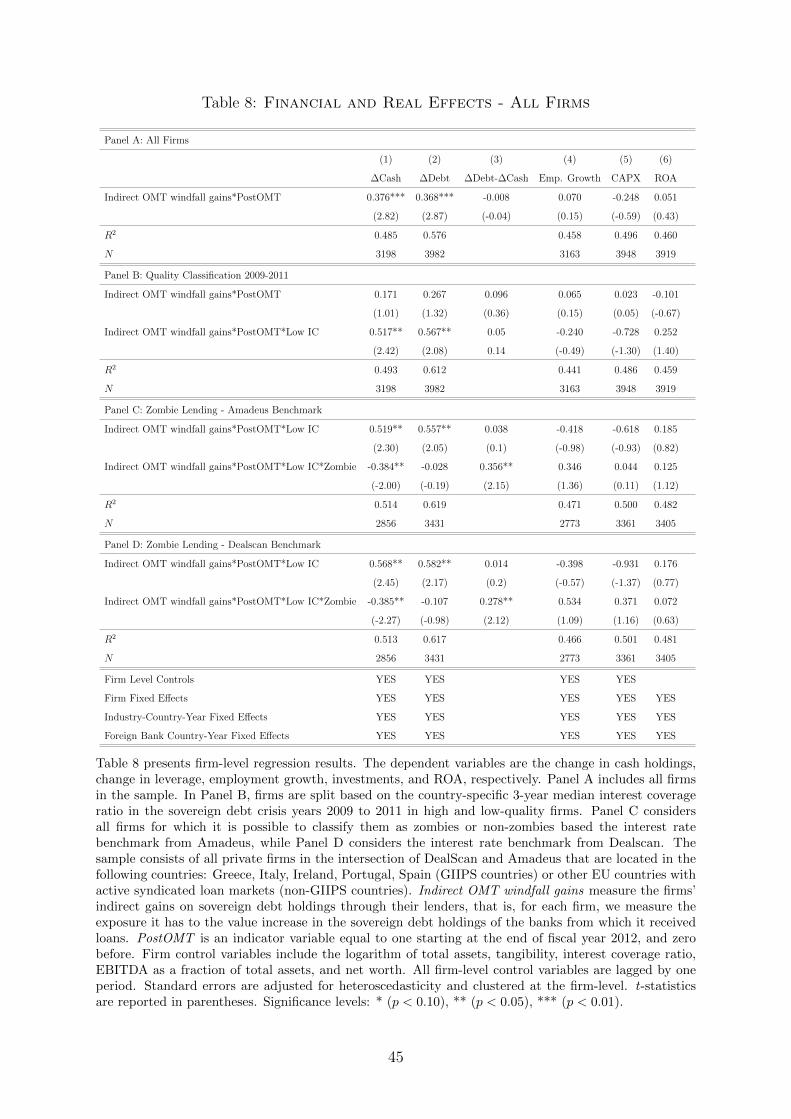
Table 8: Financial and Real Effects - All Firms

Panel A: All Firms

(1) (2) (3) (4) (5) (6)

�Cash �Debt �Debt-�Cash Emp. Growth CAPX ROA

Indirect OMT windfall gains*PostOMT 0.376*** 0.368*** -0.008 0.070 -0.248 0.051

(2.82) (2.87) (-0.04) (0.15) (-0.59) (0.43)

R2 0.485 0.576 0.458 0.496 0.460

N 3198 3982 3163 3948 3919

Panel B: Quality Classification 2009-2011

Indirect OMT windfall gains*PostOMT 0.171 0.267 0.096 0.065 0.023 -0.101

(1.01) (1.32) (0.36) (0.15) (0.05) (-0.67)

Indirect OMT windfall gains*PostOMT*Low IC 0.517** 0.567** 0.05 -0.240 -0.728 0.252

(2.42) (2.08) 0.14 (-0.49) (-1.30) (1.40)

R2 0.493 0.612 0.441 0.486 0.459

N 3198 3982 3163 3948 3919

Panel C: Zombie Lending - Amadeus Benchmark

Indirect OMT windfall gains*PostOMT*Low IC 0.519** 0.557** 0.038 -0.418 -0.618 0.185

(2.30) (2.05) (0.1) (-0.98) (-0.93) (0.82)

Indirect OMT windfall gains*PostOMT*Low IC*Zombie -0.384** -0.028 0.356** 0.346 0.044 0.125

(-2.00) (-0.19) (2.15) (1.36) (0.11) (1.12)

R2 0.514 0.619 0.471 0.500 0.482

N 2856 3431 2773 3361 3405

Panel D: Zombie Lending - Dealscan Benchmark

Indirect OMT windfall gains*PostOMT*Low IC 0.568** 0.582** 0.014 -0.398 -0.931 0.176

(2.45) (2.17) (0.2) (-0.57) (-1.37) (0.77)

Indirect OMT windfall gains*PostOMT*Low IC*Zombie -0.385** -0.107 0.278** 0.534 0.371 0.072

(-2.27) (-0.98) (2.12) (1.09) (1.16) (0.63)

R2 0.513 0.617 0.466 0.501 0.481

N 2856 3431 2773 3361 3405

Firm Level Controls YES YES YES YES

Firm Fixed E↵ects YES YES YES YES YES

Industry-Country-Year Fixed E↵ects YES YES YES YES YES

Foreign Bank Country-Year Fixed E↵ects YES YES YES YES YES

Table 8 presents firm-level regression results. The dependent variables are the change in cash holdings,change in leverage, employment growth, investments, and ROA, respectively. Panel A includes all firmsin the sample. In Panel B, firms are split based on the country-specific 3-year median interest coverageratio in the sovereign debt crisis years 2009 to 2011 in high and low-quality firms. Panel C considersall firms for which it is possible to classify them as zombies or non-zombies based the interest ratebenchmark from Amadeus, while Panel D considers the interest rate benchmark from Dealscan. Thesample consists of all private firms in the intersection of DealScan and Amadeus that are located in thefollowing countries: Greece, Italy, Ireland, Portugal, Spain (GIIPS countries) or other EU countries withactive syndicated loan markets (non-GIIPS countries). Indirect OMT windfall gains measure the firms’indirect gains on sovereign debt holdings through their lenders, that is, for each firm, we measure theexposure it has to the value increase in the sovereign debt holdings of the banks from which it receivedloans. PostOMT is an indicator variable equal to one starting at the end of fiscal year 2012, and zerobefore. Firm control variables include the logarithm of total assets, tangibility, interest coverage ratio,EBITDA as a fraction of total assets, and net worth. All firm-level control variables are lagged by oneperiod. Standard errors are adjusted for heteroscedasticity and clustered at the firm-level. t-statisticsare reported in parentheses. Significance levels: * (p < 0.10), ** (p < 0.05), *** (p < 0.01).

45

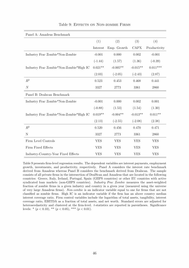
Table 9: Effects on Non-zombie Firms

Panel A: Amadeus Benchmark

(1) (2) (3) (4)

Interest Emp. Growth CAPX Productivity

Industry Frac Zombie*Non-Zombie -0.001 0.000 0.002 -0.001

(-1.44) (1.57) (1.36) (-0.39)

Industry Frac Zombie*Non-Zombie*High IC 0.021** -0.005** -0.015** 0.011***

(2.03) (-2.05) (-2.43) (2.87)

R2 0.523 0.453 0.468 0.441

N 3327 2773 3361 2860

Panel B: Dealscan Benchmark

Industry Frac Zombie*Non-Zombie -0.001 0.000 0.002 0.001

(-0.88) (1.53) (1.54) (1.30)

Industry Frac Zombie*Non-Zombie*High IC 0.019** -0.004** -0.013** 0.011**

(2.13) (-2.55) (-2.08) (2.38)

R2 0.520 0.456 0.470 0.471

N 3327 2773 3361 2860

Firm Level Controls YES YES YES YES

Firm Fixed E↵ects YES YES YES YES

Industry-Country-Year Fixed E↵ects YES YES YES YES

Table 9 presents firm-level regression results. The dependent variables are interest payments, employmentgrowth, investments, and productivity, respectively. Panel A considers the interest rate benchmarkderived from Amadeus whereas Panel B considers the benchmark derived from Dealscan. The sampleconsists of all private firms in the intersection of DealScan and Amadeus that are located in the followingcountries: Greece, Italy, Ireland, Portugal, Spain (GIIPS countries) or other EU countries with activesyndicated loan markets (non-GIIPS countries). Industry Frac Zombie measures the asset-weightedfraction of zombie firms in a given industry and country in a given year (measured using the universeof very large Amadeus firms). Non-zombie is an indicator variable equal to one for firms that are notclassified as zombie firms. High IC is an indicator variable if the firm has an above country medianinterest coverage ratio. Firm control variables include the logarithm of total assets, tangibility, interestcoverage ratio, EBITDA as a fraction of total assets, and net worth. Standard errors are adjusted forheteroscedasticity and clustered at the firm-level. t-statistics are reported in parentheses. Significancelevels: * (p < 0.10), ** (p < 0.05), *** (p < 0.01).

46

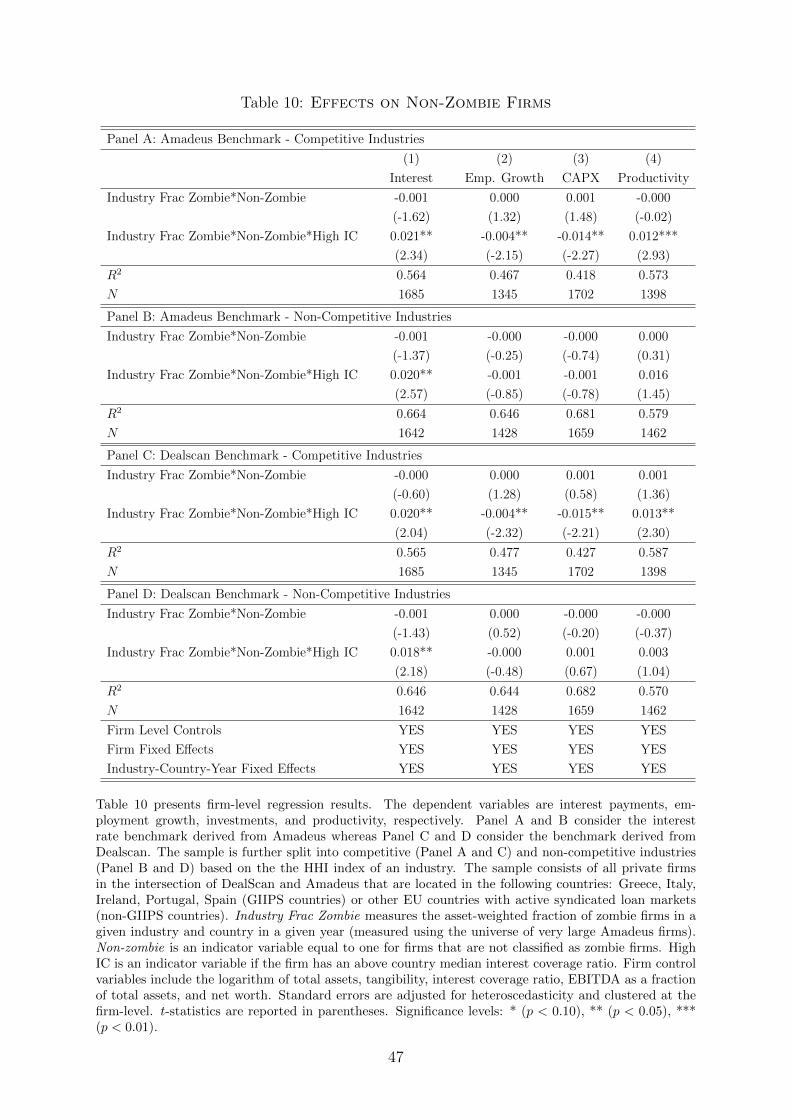
Table 10: Effects on Non-Zombie Firms

Panel A: Amadeus Benchmark - Competitive Industries

(1) (2) (3) (4)

Interest Emp. Growth CAPX Productivity

Industry Frac Zombie*Non-Zombie -0.001 0.000 0.001 -0.000

(-1.62) (1.32) (1.48) (-0.02)

Industry Frac Zombie*Non-Zombie*High IC 0.021** -0.004** -0.014** 0.012***

(2.34) (-2.15) (-2.27) (2.93)

R2 0.564 0.467 0.418 0.573

N 1685 1345 1702 1398

Panel B: Amadeus Benchmark - Non-Competitive Industries

Industry Frac Zombie*Non-Zombie -0.001 -0.000 -0.000 0.000

(-1.37) (-0.25) (-0.74) (0.31)

Industry Frac Zombie*Non-Zombie*High IC 0.020** -0.001 -0.001 0.016

(2.57) (-0.85) (-0.78) (1.45)

R2 0.664 0.646 0.681 0.579

N 1642 1428 1659 1462

Panel C: Dealscan Benchmark - Competitive Industries

Industry Frac Zombie*Non-Zombie -0.000 0.000 0.001 0.001

(-0.60) (1.28) (0.58) (1.36)

Industry Frac Zombie*Non-Zombie*High IC 0.020** -0.004** -0.015** 0.013**

(2.04) (-2.32) (-2.21) (2.30)

R2 0.565 0.477 0.427 0.587

N 1685 1345 1702 1398

Panel D: Dealscan Benchmark - Non-Competitive Industries

Industry Frac Zombie*Non-Zombie -0.001 0.000 -0.000 -0.000

(-1.43) (0.52) (-0.20) (-0.37)

Industry Frac Zombie*Non-Zombie*High IC 0.018** -0.000 0.001 0.003

(2.18) (-0.48) (0.67) (1.04)

R2 0.646 0.644 0.682 0.570

N 1642 1428 1659 1462

Firm Level Controls YES YES YES YES

Firm Fixed E↵ects YES YES YES YES

Industry-Country-Year Fixed E↵ects YES YES YES YES

Table 10 presents firm-level regression results. The dependent variables are interest payments, em-ployment growth, investments, and productivity, respectively. Panel A and B consider the interestrate benchmark derived from Amadeus whereas Panel C and D consider the benchmark derived fromDealscan. The sample is further split into competitive (Panel A and C) and non-competitive industries(Panel B and D) based on the the HHI index of an industry. The sample consists of all private firmsin the intersection of DealScan and Amadeus that are located in the following countries: Greece, Italy,Ireland, Portugal, Spain (GIIPS countries) or other EU countries with active syndicated loan markets(non-GIIPS countries). Industry Frac Zombie measures the asset-weighted fraction of zombie firms in agiven industry and country in a given year (measured using the universe of very large Amadeus firms).Non-zombie is an indicator variable equal to one for firms that are not classified as zombie firms. HighIC is an indicator variable if the firm has an above country median interest coverage ratio. Firm controlvariables include the logarithm of total assets, tangibility, interest coverage ratio, EBITDA as a fractionof total assets, and net worth. Standard errors are adjusted for heteroscedasticity and clustered at thefirm-level. t-statistics are reported in parentheses. Significance levels: * (p < 0.10), ** (p < 0.05), ***(p < 0.01).

47

For Online Publication

Online Appendix for

“Whatever it takes: The Real E↵ects of Unconventional Monetary Policy”

Viral V. Acharya

Tim Eisert

Christian Eufinger

Christian Hirsch

May 2016

48

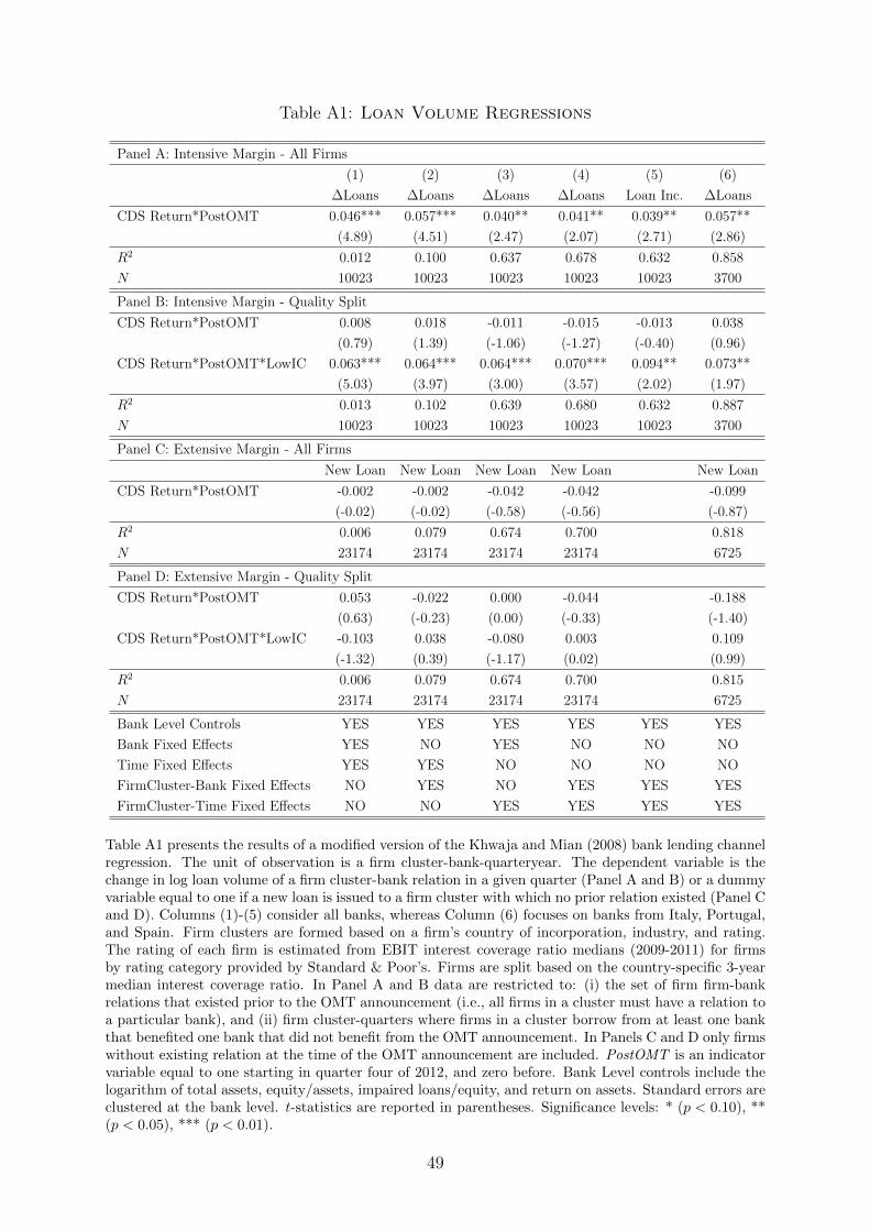
Table A1: Loan Volume Regressions

Panel A: Intensive Margin - All Firms

(1) (2) (3) (4) (5) (6)

�Loans �Loans �Loans �Loans Loan Inc. �Loans

CDS Return*PostOMT 0.046*** 0.057*** 0.040** 0.041** 0.039** 0.057**

(4.89) (4.51) (2.47) (2.07) (2.71) (2.86)

R2 0.012 0.100 0.637 0.678 0.632 0.858

N 10023 10023 10023 10023 10023 3700

Panel B: Intensive Margin - Quality Split

CDS Return*PostOMT 0.008 0.018 -0.011 -0.015 -0.013 0.038

(0.79) (1.39) (-1.06) (-1.27) (-0.40) (0.96)

CDS Return*PostOMT*LowIC 0.063*** 0.064*** 0.064*** 0.070*** 0.094** 0.073**

(5.03) (3.97) (3.00) (3.57) (2.02) (1.97)

R2 0.013 0.102 0.639 0.680 0.632 0.887

N 10023 10023 10023 10023 10023 3700

Panel C: Extensive Margin - All Firms

New Loan New Loan New Loan New Loan New Loan

CDS Return*PostOMT -0.002 -0.002 -0.042 -0.042 -0.099

(-0.02) (-0.02) (-0.58) (-0.56) (-0.87)

R2 0.006 0.079 0.674 0.700 0.818

N 23174 23174 23174 23174 6725

Panel D: Extensive Margin - Quality Split

CDS Return*PostOMT 0.053 -0.022 0.000 -0.044 -0.188

(0.63) (-0.23) (0.00) (-0.33) (-1.40)

CDS Return*PostOMT*LowIC -0.103 0.038 -0.080 0.003 0.109

(-1.32) (0.39) (-1.17) (0.02) (0.99)

R2 0.006 0.079 0.674 0.700 0.815

N 23174 23174 23174 23174 6725

Bank Level Controls YES YES YES YES YES YES

Bank Fixed E↵ects YES NO YES NO NO NO

Time Fixed E↵ects YES YES NO NO NO NO

FirmCluster-Bank Fixed E↵ects NO YES NO YES YES YES

FirmCluster-Time Fixed E↵ects NO NO YES YES YES YES

Table A1 presents the results of a modified version of the Khwaja and Mian (2008) bank lending channelregression. The unit of observation is a firm cluster-bank-quarteryear. The dependent variable is thechange in log loan volume of a firm cluster-bank relation in a given quarter (Panel A and B) or a dummyvariable equal to one if a new loan is issued to a firm cluster with which no prior relation existed (Panel Cand D). Columns (1)-(5) consider all banks, whereas Column (6) focuses on banks from Italy, Portugal,and Spain. Firm clusters are formed based on a firm’s country of incorporation, industry, and rating.The rating of each firm is estimated from EBIT interest coverage ratio medians (2009-2011) for firmsby rating category provided by Standard & Poor’s. Firms are split based on the country-specific 3-yearmedian interest coverage ratio. In Panel A and B data are restricted to: (i) the set of firm firm-bankrelations that existed prior to the OMT announcement (i.e., all firms in a cluster must have a relation toa particular bank), and (ii) firm cluster-quarters where firms in a cluster borrow from at least one bankthat benefited one bank that did not benefit from the OMT announcement. In Panels C and D only firmswithout existing relation at the time of the OMT announcement are included. PostOMT is an indicatorvariable equal to one starting in quarter four of 2012, and zero before. Bank Level controls include thelogarithm of total assets, equity/assets, impaired loans/equity, and return on assets. Standard errors areclustered at the bank level. t-statistics are reported in parentheses. Significance levels: * (p < 0.10), **(p < 0.05), *** (p < 0.01).

49

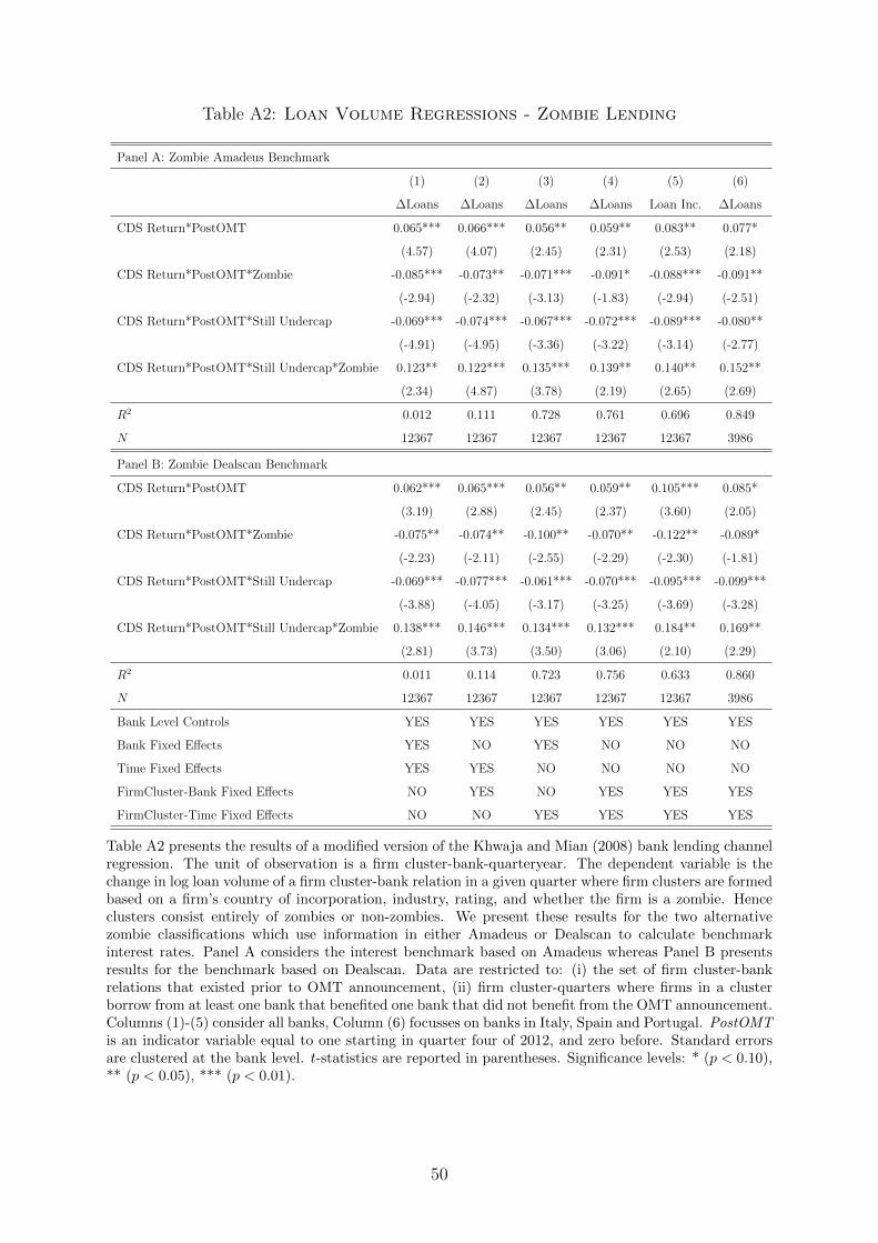
Table A2: Loan Volume Regressions - Zombie Lending

Panel A: Zombie Amadeus Benchmark

(1) (2) (3) (4) (5) (6)

�Loans �Loans �Loans �Loans Loan Inc. �Loans

CDS Return*PostOMT 0.065*** 0.066*** 0.056** 0.059** 0.083** 0.077*

(4.57) (4.07) (2.45) (2.31) (2.53) (2.18)

CDS Return*PostOMT*Zombie -0.085*** -0.073** -0.071*** -0.091* -0.088*** -0.091**

(-2.94) (-2.32) (-3.13) (-1.83) (-2.94) (-2.51)

CDS Return*PostOMT*Still Undercap -0.069*** -0.074*** -0.067*** -0.072*** -0.089*** -0.080**

(-4.91) (-4.95) (-3.36) (-3.22) (-3.14) (-2.77)

CDS Return*PostOMT*Still Undercap*Zombie 0.123** 0.122*** 0.135*** 0.139** 0.140** 0.152**

(2.34) (4.87) (3.78) (2.19) (2.65) (2.69)

R2 0.012 0.111 0.728 0.761 0.696 0.849

N 12367 12367 12367 12367 12367 3986

Panel B: Zombie Dealscan Benchmark

CDS Return*PostOMT 0.062*** 0.065*** 0.056** 0.059** 0.105*** 0.085*

(3.19) (2.88) (2.45) (2.37) (3.60) (2.05)

CDS Return*PostOMT*Zombie -0.075** -0.074** -0.100** -0.070** -0.122** -0.089*

(-2.23) (-2.11) (-2.55) (-2.29) (-2.30) (-1.81)

CDS Return*PostOMT*Still Undercap -0.069*** -0.077*** -0.061*** -0.070*** -0.095*** -0.099***

(-3.88) (-4.05) (-3.17) (-3.25) (-3.69) (-3.28)

CDS Return*PostOMT*Still Undercap*Zombie 0.138*** 0.146*** 0.134*** 0.132*** 0.184** 0.169**

(2.81) (3.73) (3.50) (3.06) (2.10) (2.29)

R2 0.011 0.114 0.723 0.756 0.633 0.860

N 12367 12367 12367 12367 12367 3986

Bank Level Controls YES YES YES YES YES YES

Bank Fixed E↵ects YES NO YES NO NO NO

Time Fixed E↵ects YES YES NO NO NO NO

FirmCluster-Bank Fixed E↵ects NO YES NO YES YES YES

FirmCluster-Time Fixed E↵ects NO NO YES YES YES YES

Table A2 presents the results of a modified version of the Khwaja and Mian (2008) bank lending channelregression. The unit of observation is a firm cluster-bank-quarteryear. The dependent variable is thechange in log loan volume of a firm cluster-bank relation in a given quarter where firm clusters are formedbased on a firm’s country of incorporation, industry, rating, and whether the firm is a zombie. Henceclusters consist entirely of zombies or non-zombies. We present these results for the two alternativezombie classifications which use information in either Amadeus or Dealscan to calculate benchmarkinterest rates. Panel A considers the interest benchmark based on Amadeus whereas Panel B presentsresults for the benchmark based on Dealscan. Data are restricted to: (i) the set of firm cluster-bankrelations that existed prior to OMT announcement, (ii) firm cluster-quarters where firms in a clusterborrow from at least one bank that benefited one bank that did not benefit from the OMT announcement.Columns (1)-(5) consider all banks, Column (6) focusses on banks in Italy, Spain and Portugal. PostOMTis an indicator variable equal to one starting in quarter four of 2012, and zero before. Standard errorsare clustered at the bank level. t-statistics are reported in parentheses. Significance levels: * (p < 0.10),** (p < 0.05), *** (p < 0.01).

50