employment e ects of unconventional monetary … contrast, after qe1, no such differential effect is...

Finance and Economics Discussion SeriesDivisions of Research & Statistics and Monetary Affairs

Federal Reserve Board, Washington, D.C.

Employment effects of unconventional monetary policy: Evidencefrom QE

Stephan Luck and Tom Zimmermann

2018-071

Please cite this paper as:Luck, Stephan, and Tom Zimmermann (2018). “Employment effects of unconven-tional monetary policy: Evidence from QE,” Finance and Economics Discussion Se-ries 2018-071. Washington: Board of Governors of the Federal Reserve System,https://doi.org/10.17016/FEDS.2018.071.

NOTE: Staff working papers in the Finance and Economics Discussion Series (FEDS) are preliminarymaterials circulated to stimulate discussion and critical comment. The analysis and conclusions set forthare those of the authors and do not indicate concurrence by other members of the research staff or theBoard of Governors. References in publications to the Finance and Economics Discussion Series (other thanacknowledgement) should be cleared with the author(s) to protect the tentative character of these papers.

Employment effects of unconventional monetary policy:Evidence from QE∗

Stephan Luck†and Tom Zimmermann‡

Federal Reserve Board, University of Cologne

October 9, 2018

Abstract

This paper investigates the effect of the Federal Reserve’s unconventional monetary policy onemployment via a bank lending channel. We find that banks with higher mortgage-backed securitiesholdings made relatively more loans after the first and third rounds of quantitative easing (QE1 andQE3). While additional volume is concentrated in refinanced mortgages after QE1, increases aredriven by newly originated home purchase mortgages and additional commercial and industriallending after QE3. Using spatial variation, we show that regions with a high share of affected banksexperienced stronger employment growth after both QE1 and QE3. While the ability of householdsto refinance mortgages after QE1 spurred local demand, the resulting additional employment growthwas relatively weak and confined to the non-tradable goods sector. In contrast, the increase inemployment after QE3 is sizable and can be attributed to the supply of additional credit to firms.To support this finding, we use new confidential loan-level data to show that firms with strongerties to affected banks increased employment and capital investment more after QE3. Altogether, ourfindings suggest that unconventional monetary policy can, similar to conventional monetary policy,affect real economic outcomes.

∗This paper presents the view of the authors and not of the Federal Reserve. We would like to thank David Arseneau, JoseBerrospide, Neil Bhutta, David Byrne, Daniel Cooper, Olivier Darmouni, Cynthia Doninger, Burcu Duygan-Bump, MiguelFaria-e-Castro, Michael Connolly, Giovanni Favara, Andreas Fuster, Paul Goldsmith-Pinkham, Simon Jaeger, Elizabeth Klee,Arvind Krishnamurthy, Anna Kovner, Adrien Matray, Michael McMahon, Ralf Meisenzahl, Atif Mian, John Mondragon,Christopher Palmer, Matthew Plosser, Farzad Saidi, Eric Swanson, Skander van den Heuvel, Joe Vavra, James Vickery, EgonZakrasjek as well as seminar participants at the 2017 NBER Monetary Economics Program meeting, Federal Reserve Bankof New York, Federal Reserve Board, Federal Reserve Bank of St. Louis, MFA San Antonio, EABCN Barcelona, BarcelonaSummer Forum on Monetary Policy and Central Banking, ITAM Finance, University College Dublin, CEBRA Frankfurt forhelpful comments and suggestions. We thank Zach Fernandes and Tyler Wake for excellent research assistance.

†Federal Reserve Board, [email protected]‡University of Cologne, [email protected]

1

1 Introduction

Does unconventional monetary policy affect the real economy? And if so, what are the channels?

Over the course of the 07-08 Financial Crisis, monetary policy reached the zero lower bound in several

countries. As a consequence, central banks have turned toward unconventional monetary policies

such as forward guidance and large-scale asset purchases (LSAPs). Because the channels through

which unconventional monetary policy affects the real economy are yet not fully understood and

because conclusive empirical evidence is scarce, the efficacy and desirability of such policies has been

controversial.1

Against this background, this study investigates the real effects of the Federal Reserve’s uncon-

ventional monetary policy. Our study is the first to document a link between the Federal Reserve’s

quantitative easing (QE) and employment outcomes. This is a particularly important finding as previous

research has highlighted an effect of QE on bank lending (Darmouni and Rodnyansky, 2017), and an

effect of QE on household net-worth and consumption via the mortgage market (Di Maggio et al., 2016;

Beraja et al., 2018), but has not been able to speak to the crucial question of its effect on improving

broader economic conditions such as employment outcomes.

In particular, we show that while the first round of QE (QE1) led to increased refinancing activity in

the mortgage market by commercial banks, this additional lending activity had only weak effects on

employment growth, confined to the non-tradable goods sector. In contrast, the third round of QE (QE3)

induced additional commercial and industrial (C&I) lending as well as increased origination of home

purchase mortgages, which in turn translated into economically sizable growth in total employment.

Our evidence suggests that LSAPs can, similar to reductions of interest rates in times of conventional

monetary policy, affect real economic outcomes via a bank lending channel.2

The empirical assessment of macroeconomic policy is generally difficult, given the natural absence

of a control group.3 In order to overcome this inherent challenge, we proceed in three steps. First, we

1For instance, after the implementation of QE1 a number of prominent economists wrote an open letter to Ben Bernanke(published in the Wall Street Journal on November 15 2010): “We believe the Federal Reserve’s large-scale asset purchase plan(so-called ‘quantitative easing’) should be reconsidered and discontinued. We do not believe such a plan is necessary oradvisable under current circumstances. The planned asset purchases risk currency debasement and inflation, and we do notthink they will achieve the Fed’s objective of promoting employment.”

2Given that we do not identify strong employment effects of QE1 and QE2 does not imply that these programs didn’t haveconsiderable impact on the real economy via different channels not considered in this paper. Likewise, given the cross-sectionalnature of our analysis, one cannot easily draw conclusions with respect to aggregate employment.

3The problem is best summarized by Ben Bernanke in his memoir, The Courage to Act: “We can’t know exactly how much ofthe U.S. recovery can be attributed to monetary policy, since we can only conjecture what might have happened if the Fed hadnot taken the steps that it did.”

2

exploit cross-sectional variation in the exposure of commercial banks to QE. Second, we exploit spatial

variation in the activity of banks that were more affected by QE, allowing us to trace the effect of QE on

local credit and labor markets. Third, we use confidential loan-level and mortgage-level credit registry

data that allow us to shed light on whether additional credit results from changes in credit supply or

credit demand.

In the first step, we exploit a link between QE and bank lending that has recently been established in

several papers (see, e.g. Darmouni and Rodnyansky, 2017). This literature uses cross-sectional variation

of banks’ mortgage-backed securities (MBS) holdings in order to identify an effect of QE on bank

lending. Complementary to these findings, we show that more exposed banks experienced higher stock

returns on QE announcement days, controlling for many potentially confounding bank characteristics.

In addition, we find that, within the mortgage market, QE1 mainly affected the refinancing volume of

existing mortgages (Di Maggio et al., 2016; Beraja et al., 2018), and QE3 affected the origination of home

purchase mortgages at more exposed banks. Within the C&I loan market, only QE3 increased lending,

in particular in to smaller firms. These findings turn out to be important for understanding how QE

affected employment.

In the second and central part of the paper, we study the link between bank lending and employment

at the county level. We exploit that, on top of the cross-sectional variation of MBS holdings, there is

geographical variation in banks’ activity. Importantly, a bank’s regions of activity are very stable over

time and highly predictable. Measuring banks’ local activity by either the historical amount of small

business lending, mortgage origination, or deposit volume in a given county, we construct an exposure

measure at the county level: We treat counties that have historical activity from banks with more MBS

holdings as exposed counties and those with less activity from such banks as non-exposed counties.

A concern with our approach is that banks with higher MBS might systematically select into markets

that are most economically developed, or that are expected to display high future economic growth. Our

identification addresses this concern in two ways. First, while banks’ location choices are systematic, they

are also highly persistent. It is hence unlikely that banks selected locations in anticipation of quantitative

easing, and it is such correlation with the timing of unconventional monetary policy that would be of

most concern. Second, our difference-in-differences approach allows for systematic differences across

markets as long as markets would have co-moved in absence of QE. We provide evidence in support of

this assumption.

In particular, employment growth in counties with high and low exposure to banks with large MBS

3

holdings evolved very similarly during the Financial Crisis, suggesting that these counties were on

similar trajectories absent QE. To be precise, employment growth in exposed and non-exposed counties

followed the same trend for more than 18 consecutive quarters before the implementation of QE3. After

QE3, however, we find that exposed counties experience higher overall employment growth. The effects

are economically sizable: Our estimates suggest that counties in the upper tercile of the MBS–bank

distribution experienced 40 basis points higher employment growth than counties in the lower tercile of

the distribution. In contrast, after QE1, no such differential effect is observed. While exposed counties

do experience higher employment growth in the non-tradable goods sector during QE1, the effect is

weak, and overall employment growth is statistically indistinguishable between affected and unaffected

counties.

Finally, in the third step, we analyze whether additional credit is driven by changes in credit

supply as opposed to credit demand. In order to control for demand in the C&I loan market, we use

newly available confidential loan–level data from the Y-14 data collection, which, since 2011, requires

large banks with more than $50 billion in assets to report any C&I loan on their balance sheet with a

commitment of 1 million USD or more.

Using the loan-level database, we provide evidence that the increase in lending after QE3 is not

driven by increases in demand for loans by firms, but rather by additional supply of bank loans.

To account for loan demand by firms, we control for firm-specific demand in the spirit of Khwaja

and Mian (2008) in bank–firm–level regressions. Moreover, using firm-level data on investment and

employment, we provide evidence that, after QE3, firms that historically tended to borrow from affected

banks increased capital investment and employment by more than firms that had been borrowing from

unaffected banks. Notably, our results in this part contrast to results documented by Chakraborty et al.

(2016), who find a negative effect of QE3 on C&I credit and investment by large firms. The difference in

findings can largely be explained by the fact that our data also contains medium-sized firms that are not

active in the syndicated loan market. In particular, we show that the increased volume of C&I lending is

more pronounced for non-syndicated borrowing by medium sized firms than for syndicated borrowing

from larger firms, consistent with larger firms being less bank dependent.

In order to control for credit demand in the mortgage market, we use confidential mortgage-level data.

In particular, we exploit that multiple banks are active in the same county and account for local credit

demand by households by controlling for county-specific demand in county–bank–level regressions. We

show that after QE1 was implemented, affected banks are more likely to refinance mortgages irrespective

4

of whether they are GSE-conforming or non-conforming. However, when controlling for local demand,

the effect becomes weaker in its magnitude, in particular for GSE-conforming mortgages, but remains

statistically significant. We interpret this as evidence that the increase in refinancing activity after QE1 is

partially driven by increased credit supply, complementary to the findings by Di Maggio et al. (2016)

and Beraja et al. (2018), who emphasize the demand of households to refinance mortgages after QE1.

While our results indicate that the increase in lending stems from an increase in credit supply to

households as well as firms, the employment effect could be the result of two separate channels: It

could either result from an increase in local credit supply to firms, or from increased local credit supply

to households, which in turn affects employment through increasing demand for local consumption.

While generally both channels may be relevant, our data gives us some sense of which type of lending

is more important for employment. In particular, we exploit that increases in demand are more likely to

affect the non-tradable goods sector than the tradable goods sector. Hence, if increased demand was

driving the increase in economic activity, additional employment would more likely be generated in the

non-tradable goods sector (Mian and Sufi, 2014).

Even though we do not find an effect on total employment during QE1, employment in the non-

tradable sector increases subsequent to the implementation of the program. Moreover, the increase in

employment in the non-tradable sector coincides with an increase in auto sales, which are a proxy for

overall household consumption. Our findings thus suggest that the ability of households to refinance

mortgages after QE1 spurred local demand for consumption by increasing household net-worth,

resulting in increased employment in the non-tradable goods sector.

In contrast, we find that the overall change in employment after QE3 is driven by changes of

employment in sectors other than the non-tradable goods sector. We argue that the significant increase

in employment after QE3 is more likely to be a consequence of the increased supply of C&I loans rather

than increased mortgage origination, consistent with increases in lending, investment and employment

at firms with relationships to more exposed banks as discussed above.

Our results survive a large number of additional tests. First, the second round of QE (QE2) consisted

entirely of Treasury purchases, and hence acts as a natural placebo test: Indeed, we do not find a

significant relation between MBS exposure and bank lending or employment following QE2. Second, if

QE3 induced bank lending and employment, the tapering of QE3 should have effects in the opposite

direction: We provide evidence that supports this conjecture. Finally, we also show that our main results

are robust to minor variations in the empirical specification and sample restrictions.

5

Altogether, our findings suggest that unconventional monetary policy can, similar to conventional

monetary policy, spur economic activity via a bank lending channel. In particular, LSAPs can induce

commercial banks to expand lending which may translate into additional employment. However,

differences in findings across the different rounds of QE suggest that the effects are time varying,

mirroring findings on the effects of conventional monetary policy (Vavra, 2014).

We proceed as follows. After a brief summary of the existing literature, Section 2 discusses data

used in our study. Section 3 presents the empirical strategy and discusses results on bank lending and

employment.Section 4 separates supply and demand effects in the C&I loan and mortgage markets

using loan-level data. Section 5 discusses evidence from additional events (QE2 and tapering) and

robustness of results before we conclude in Section 6.

1.1 Related literature

Our study contributes to the literature on the bank lending channel of monetary policy. During times of

conventional monetary policy, the conventional wisdom is that more accommodative monetary policy

is associated with an increase in bank lending and a decrease in unemployment (see, e.g. Bernanke

and Blinder, 1992; Kashyap and Stein, 1994, 2000; Drechsler et al., 2017). Previous studies on the effect

of unconventional monetary policy in the United States have mostly focused on outcomes other than

employment. For instance, recent studies have investigated the effects of QE on aggregate financing

cost (Hancock and Passmore, 2011; Gilchrist et al., 2015) or on outcomes in the housing market and

at the household level (Di Maggio et al., 2016; Beraja et al., 2018), at the bank level (Darmouni and

Rodnyansky, 2017; Kurtzman et al., 2017), or at the firm level (Foley-Fisher et al., 2016; Chakraborty

et al., 2016).4

Our analysis of bank lending is closely related to Darmouni and Rodnyansky (2017) and Di Maggio

et al. (2016), who exploit cross-sectional variation in MBS holdings. Darmouni and Rodnyansky (2017)

document a positive effect of QE1 and QE3 on bank lending using Call Report data. While the focus of

our study is on employment outcomes, we also provide complementary bank-level evidence beyond

their study by distinguishing more granularly between different types of lending, and by investigating

stock market reactions to QE announcements.

Di Maggio et al. (2016) and Beraja et al. (2018) study the effect of QE on the mortgage market in

4There are also several papers that investigate the effects of unconventional monetary policy in Europe (see, e.g., Acharyaet al., 2016; Carpinelli and Crosignani, 2017; Crosignani et al., 2018; Cahn et al., 2018; Cumming, 2018).

6

more detail. In particular, Di Maggio et al. (2016) show that the Federal Reserve’s purchases of MBS are

associated with a refinancing boom after QE1, which in turn triggered significant equity extraction and

an increase in consumption. Beraja et al. (2018) show that refinancing and the subsequent growth in

consumption is more pronounced in regions in which households have lower leverage and are hence

less constrained in their refinancing decision. Both is consistent with the employment increase in the

non-tradables sector that we document. Importantly, however, this employment effect is modest and

does not translate into an effect for overall employment. As we document, only the additional lending

subsequent to QE3 had a significant effect on overall employment and is arguably driven by credit

supply rather than credit demand.

Foley-Fisher et al. (2016) and Chakraborty et al. (2016) study the effect of unconventional monetary

policy on firm behavior. In particular, Foley-Fisher et al. (2016) investigate the effects of the monetary

expansion program (MEP), on non-financial firms and they find that firms that historically relied more

on long-term debt issued more long-term debt after the MEP and that those firms increased investment.

Chakraborty et al. (2016) study the effect of QE on bank lending and firm investment. While we

find that QE3 induced additional C&I lending, Chakraborty et al. (2016) find that QE crowded out C&I

lending and led to a reduction of investment by large firms. The differences in findings can be explained

by the difference in the empirical specification and by differences in data coverage. First, their findings

suggest a negative relationship between mortgage lending and C&I lending over a longer period, in line

with more general trends documented by Chakraborty et al. (2018). In contrast, our findings suggest

that, specifically around QE3, banks conduct additional mortgage lending as well as additional C&I

lending. Second, our confidential loan-level data are less restricted in two important aspects: Our

C&I lending data are not restricted to syndicated loans alone, and our sample at the bank-firm level

is substantially larger and likely more representative of the C&I lending landscape. We find that the

effect of QE3 is stronger for smaller firms that are not active in the syndicated loan market and that are

arguably more bank dependent. Second, our data on C&I lending as well as our data on mortgages is at

the quarterly rather than annual frequency and therefore allows us to capture the timing of QE effects

more precisely.

More generally, our analysis of the employment effects of QE contributes to the literature on how

financial conditions affect real economic outcomes (see, e.g., Bernanke, 1983; Peek and Rosengren, 2000;

Driscoll, 2004; Khwaja and Mian, 2008). In particular, a series of recent papers show how the 2007-08

financial crisis affected bank lending (see, e.g., Ivashina and Scharfstein, 2010), and real economic

7

outcomes via various lending channels (see, e.g., Chodorow-Reich, 2014; Duygan-Bump et al., 2015;

Haltenhof et al., 2014; Bord et al., 2015; Benmelech et al., 2017; Greenstone et al., 2015). Our empirical

strategy is closest to Benmelech et al. (2017), Bord et al. (2015), or Greenstone et al. (2015), who exploit

spatial variation in the exposure to the financial crisis. Unlike our paper, which is concerned with the

effect of unconventional monetary policy on employment, Benmelech et al. (2017) trace the effect of the

run in the asset-backed commercial paper market on auto sales, and Bord et al. (2015) and Greenstone

et al. (2015) analyze the employment effects of the financial crisis through reductions in small business

lending.

2 Data

Our study brings together data from different sources at the bank, county, and firm level.

We take commercial bank balance sheet and income statement information from the Consolidated

Reports of Condition and Income for commercial banks in the United States (Call Reports, based on

Forms FFIEC 031 and FFIEC 041). Information on bank holding companies are obtained from the the

Consolidated Financial Statements for Holdings Companies (FR Y-9C). All items are adjusted for bank

mergers. We match publicly traded BHC’s with daily stock returns from the Center for Research in

Security Prices (CRSP) using the publicly available crosswalk provided by the Federal Reserve Bank of

New York.

We make use of three further administrative sources that collect data on bank lending. The Home

Mortgage Disclosure Act (HMDA) requires most banks to report on their mortgage lending activity.

Data are reported at the mortgage-level and include information on the mortgage amount, whether the

amount refers to the origination of a mortgage for a home purchase or the re-financing of an existing

loan, and the geographic location of the property down to the census tract level. Virtually all banks in

the Unites States that conduct any mortgage lending in an MSA report on their activity, so the HMDA

data are considered a near census of mortgage lending. Importantly, the public version of the HMDA

data only identifies the year of the observation. We use a confidential version of the data, maintained by

the Board of Governors of the Federal Reserve, that reports exact application and action dates for each

observation and therefore enables us to measure the timing of potential lending effects more precisely.

For our analysis, we aggregate the HMDA data to the bank-quarter level and to the county-quarter level.

Similar to the HMDA data, the Community Reinvestment Act (CRA) requires banks to report on

8

small business lending activity by geographic area. Each bank breaks down data by geographic region

down to the census tract and by loan size bins. In addition, banks report total lending to businesses

with revenues of less than $1m. The CRA data are fairly representative of the universe of small business

lending by commercial banks: Greenstone et al. (2015) estimate that small business lending in the CRA

data captures 86% of total small business lending in the U.S.

In addition, we use data from the Summary of Deposits (SoD) collected by the Federal Deposit

Insurance Corporation (FDIC). The SoD data consist of annual branch-level reports of total deposits by

bank branch, and we aggregate the data to the bank–county level in our analysis.

County-level data come from different sources. Employment data are from the Quarterly Census of

Employment and Wages (QCEW) that is collected by the Bureau of Labor Statistics. The data provide

quarterly counts of employment and wages by industry as reported by employers, and they cover more

than 95% of U.S. jobs. We complement employment data with the County Business Patterns (CBP), an

annual data collection by the U.S. Census that includes the number of establishments and number of

employees by industry and county in the first week of March each year. The CBP data often report

employment only in brackets. We use the method in Autor et al. (2013) to estimate employment numbers

within brackets. As additional data on local economic conditions, we obtain regional house prices from

Moody’s, median income from Haver Analytics, auto sales data from Polk, and population from the U.S.

Census.

To investigate directly the link between banks’ MBS holdings, corporate lending and real outcomes

for a subset of banks and firms, we make use of newly available administrative data on bank loans. Since

2012, regulators have collected loan-level data on bank lending from any bank with total assets of more

than 50 billion USD on a quarterly basis. The purpose of the data collection is to assess capital adequacy

and to support stress test models, and the loan schedule (Y-14Q-H1) requires banks to report any loan

on their balance sheet with a commitment of 1 million USD or more. Data include loan characteristics

such as interest rates and the dates on which those rates can be re-set, collateral requirements, and the

purpose of the loan. Moreover, the data allow to distinguish between term loans and credit lines, and

whether a loan is syndicated or not; and include borrower characteristics, such as total assets, total debt,

and capital investment. Firms can be followed across banks in the data set by their tax identification

numbers. Importantly, relative to other data sets (such as DealScan or SNC), this data set includes

syndicated loans but also many smaller and/or non-syndicated loans, and therefore has much broader

coverage of firms than has been available in previous studies.

9

When we look at employment effects at the firm-level, we match the loan registry data with firms’

annual employment figures from Compustat based on tax identification numbers. Analysis of firm-level

employment effects is therefore restricted to firms that can be matched in both datasets, and the overlap

amounts to roughly 2700 companies.

3 Evidence on lending and employment

3.1 Empirical Strategy

We exploit two sources of variation to study the effect of unconventional monetary policy on employment

via bank lending: First, we use the fact that banks were arguably differentially exposed to the Fed’s MBS

purchases during QE1 and QE3, which led to differential lending responses at the bank level. Second,

banks’ business activities vary across different regions, allowing us to investigate how local changes in

bank lending correlate with changes in employment.

We start out by briefly5 reviewing the Federal Reserve’s unconventional monetary policy before

laying out our empirical strategy in more detail.

3.1.1 The Federal Reserve’s LSAPs

By the end of 2008, the federal funds target rate effectively hit the zero lower bound, and LSAPs

became an important tool for the Federal Open Market Committee (FOMC) to conduct monetary policy.

On November 25, 2008, the FOMC announced what came to be known as QE1: the Federal Reserve

would buy up to $100 billion of direct debt obligations issued by Fannie Mae and Freddie Mac, and an

additional $500 billion of agency MBS. The program was extended in the FOMC meeting on March 18,

2009, and, by the end of QE1 (March 2010), the Federal Reserve had bought $1.25 trillion in MBS, $175

billion in Federal Agency debt, and $300 billion in U.S. Treasuries. In March 2010, the Fed held about

one quarter of all available MBS.

Over the course of 2010 and 2011 the Federal Reserve implemented two additional programs focused

solely on the purchase of Treasuries. First, on August 10, 2010, the FOMC indicated the start of a

second round of quantitative easing (QE2), which ultimately led to the total purchase of $778 billion

in long-term Treasury securities. Second, on September 21, 2011, the Federal Reserve announced the

5For a more detailed chronology of events, see Table 1 in Gilchrist et al. (2015).

10

maturity extension program (MEP), which involved the sale of short-term U.S. Treasuries and the

purchase of long-term Treasuries.

Given disappointing economic activity and still relatively high unemployment, the FOMC announced

a third round of quantitative easing (QE3) in its statement on September 13, 2012. Largely unanticipated,

QE3 initially dictated the purchase of $40 billion in agency MBS per month, and another $45 billion in

U.S. Treasuries (added to the policy on December 12, 2012). After improvements of the economy became

apparent, Chairman Ben Bernanke first indicated the Tapering of QE3 in his testimony to the Joint

Economic Committee on May 22, 2013. The potential tapering was confirmed in the FOMC statement

on June 19, 2013, and the Federal Reserve reduced the purchase amounts to $35 billion in agency MBS

and $40 billion in U.S. Treasuries, respectively in December, 2013, and the program formally ended on

October 29, 2014.

3.1.2 Variation at the bank level

In this study, we focus on the effect of the Federal Reserve’s purchases of MBS during QE1 and QE3. We

use cross-sectional variation of banks’ mortgage-backed securities (MBS) holdings in order to identify

an effect of QE on bank lending. In particular, we argue that those banks that held more MBS prior to

QE were relatively more affected by the MBS purchases.

There are several reasons to believe that large-scale purchases of agency MBS affected banks with

relatively larger MBS holdings more than banks with relatively lower MBS holdings. First, differences in

MBS holdings may capture differences in banks’ business models. Some banks tend to be more active in

the mortgage market and are thereby more exposed to housing in general. Hence, when the Federal

Reserve purchases agency MBS and the prospects of the housing market arguably rise, banks that are

more exposed to the housing market may benefit more.

Second, large-scale purchases of MBS may directly raise the values and liquidity of banks’ MBS

holdings; for theoretical mechanisms see, e.g., Gertler and Karadi (2011) and Brunnermeier and Sannikov

(2014). Krishnamurthy and Vissing-Jorgensen (2013) show that the Fed’s actions had a considerable

effect on MBS prices, especially during QE1. Moreover, they argue that QE operated through a “narrow

channel” and MBS prices changed more than other asset prices. Thus, one may argue that banks with

higher MBS shares benefited relatively more from the Fed’s actions. In line with this evidence, Darmouni

and Rodnyansky (2017) find that additional lending after QE1 stems from an improved capital position

of affected banks, and that additional lending after QE3 was driven by an improved liquidity position.

11

Third, the increase in lending may be the result of a more general portfolio re-balancing channel:

given that low-yield assets, such as reserves, are not perfect substitutes for higher yielding assets, such

as MBS, large increases in the supply of central bank money can induce banks to invest in more higher

yielding assets. This can be achieved, for instance, by issuing new loans or mortgages.

In a first step, we test the empirical connection between banks’ MBS holdings and MBS purchase

announcements by the Federal Reserve. Mirroring the approach used by Foley-Fisher et al. (2016) to

analyze the effect of the MEP on non-financial firms, we investigate stock returns of bank holding

companies on the day of the announcement of a given round of QE using the following model:

rbt = α + β

(MBS

Total Assets

)(j)

b+ θXbt + εbt (1)

where rbt is the (risk-adjusted) stock return of bank b on day t. We proxy a bank’s exposure to QE by

a bank’s share of agency MBS holdings relative to total assets,( MBS

Total Assets

)(j)b , averaged over the four

quarters prior to round j = 1, 2, 3 of QE. Xbt is a vector of bank-level characteristics available at time t.

On average, around 8% of all bank assets are MBS (see Section A in the appendix for details). In

2008, prior to QE1, more than a quarter of all commercial banks held no MBS at all, and the average

MBS-to-assets ratio was around 12% in the upper quartile of the cross-sectional distribution across

banks. Among the set of publicly traded bank holding companies, the average MBS-to-assets ratio is

around 6.5 percent in the 25th percentile and around 17 percent in the 75th percentile. Moreover, bank

with larger MBS holdings tend to be larger, more leveraged, and more exposed to the housing market in

general – observable characteristics we control for in Equation (1).

Table 1 shows estimates of equation (1) on the announcement days of QE1 and QE3, respectively. A

higher MBS share is associated with higher raw and risk-adjusted returns: In particular, the stock return

of a bank at the 75th percentile of the cross-sectional MBS share distribution exceeded the stock return of

a bank at the 25th percentile of the distribution by about 78 basis points when QE1 was announced and

by about 25 basis points when QE3 was announced, controlling for other observable bank characteristics.

These findings suggest that the market valued MBS exposure beyond e.g. bank size or leverage on QE

announcement days.

[TABLE 1 ABOUT HERE]

Figure 1 plots coefficient estimates of β when we estimate equation (1) for five days before and

12

after the announcements of QE1 and QE3. In line with QE1 occurring in a period of higher volatility,

coefficients in QE1 are less precisely estimated. Both panels suggest that banks with a higher MBS share

outperformed banks with a lower MBS share on or shortly after the day of the announcement of QE1

and QE3, respectively.

[FIGURE 1 ABOUT HERE]

Further evidence for the empirical connection between banks’ MBS holdings and the MBS purchases

of the Federal Reserve comes from the response of bank balance sheets after the implementation of the

policy. In appendix A, we find that banks that held more MBS prior to QE expanded their lending more

after the implementation of QE1 and QE3. Our analysis there, which builds on a previous study by

Darmouni and Rodnyansky (2017), shows that overall bank lending volumes increased after both, QE1

and QE3, but C&I lending increased only after QE3 and not after QE1. Within the mortgage market, QE1

mainly affected the refinancing volume of existing mortgages, in line with the findings of Di Maggio

et al. (2016), and QE3 affected the origination of home purchase mortgages at more exposed banks.

3.1.3 Variation at the regional level

Building on the empirical link between banks and the Federal Reserve’s MBS purchases described above,

we exploit that there is spatial variation in the local activity of banks with different MBS holdings. This

allows us to test whether the activity of affected bank correlates with increased local lending subsequent

to a round of QE, and whether an increase in lending correlates with employment and consumption

growth.

For our main specification, we observe counties at different points in time (quarterly or annually)

and we calculate the exposure of each county c to a round QE j as

Exposure(j)c = ∑

bw(j)

bc

(MBS

Total Assets

)(j)

b. (2)

Here, w(j)bc describes the market share of bank b in county c prior to QEj, where market share is

computed as bank b’s deposits, its volume of small business lending or its volume of mortgage lending

in county c prior to QEj relative to the total deposits (or total small business loans, or total mortgage

lending) of all banks active in county c. In other words, a county’s exposure is a bank-activity weighted

13

average of banks’ exposure to QE where a bank’s exposure is measured by its MBS holdings. Note that

since MBS are held by the respective commercial bank, the MBS share varies only at the bank-level and

not at the bank-county level.

In our main specifications, we use the exposure measure that is most closely related to the outcome

of interest, e.g. when the outcome is mortgage growth, we use the exposure measure based on mortgage

volume. In general, results are robust to using different exposure measures. As one would expect,

all three measures are highly correlated, with raw correlations being above .5 and rank correlations

being above .8. Figure B.2 in the appendix shows scatter plots of the three exposure measures based on

deposits, small business lending and mortgage lending, respectively.

Figure 2 shows our measure based on small business lending across U.S. counties before QE1. The

spatial distribution does not seem to follow a systematic pattern, except for a cluster of counties with

higher values of the exposure variable in the north east. In robustness checks, we show that results

do not depend on including the north east in the estimations. Moreover, note that since MBS shares

are very persistent within banks over time (see, e.g., Kurtzman et al., 2017) and spatial variation in

geographical activity of banks is very stable over time as well, the map looks very similar at other points

in time.


Note that our exposure measure is, however, correlated with several observable county characteristics.

Splitting the sample into the upper and lower tercile, Table 2 shows that those counties that are arguably

more affected tend to be more urban counties. Hence they have a higher population, a higher median

income, higher housing price levels and higher recent population growth. However, reassuring for our

identification strategy, both types of counties experienced comparable declines in house prices and

income during the financial crisis.


In our main analysis we estimate the following difference-in-differences specifications around the

14

first and third round of quantitative easing:

yct = α + β × Exposure(j)c × QE(j)

t + γc + τt +K

∑k=1

θ(0)k X(k)

ct +K

∑k=1

θ(1)k X(k)

ct QE(j)t + εct (3)

yct = α + β × Treat(j)c × QE(j)

t + γc + τt +K

∑k=1

θ(0)k X(k)

ct +K

∑k=1

θ(1)k X(k)

ct QE(j)t + εct (4)

Here, yct is an outcome in county c at time t, and γc and τt denote county and time fixed effects.

QE(j)t is a dummy variable equal to 1 in all time periods after QEj and 0 otherwise. Equation (3) uses

the continuous exposure measure directly, while Equation (4) uses a binary version with Treat(j)c equal

to 1 if a county’s exposure is in the upper tercile of the exposure distribution over all counties, and 0

if it is in the lower tercile of that distribution. X(k)ct is a vector of county-level time-varying controls,

including levels and annual growth of population and median income. We allow for changes in the

relation between controls and outcome variables in response to QE by interacting control variables with

QE event dummies. Also note that we restrict data to counties with a population no less than 2500

registered inhabitants, as data from such small counties are less reliable.

We estimate our main equation for three different types of outcomes at the county level. First,

we consider the effect on local lending, distinguishing between mortgage lending to households and

lending to firms, the latter proxied by small business lending. Second, in our main analysis, we consider

the effect on local employment. Finally, we investigate the effect on local employment by different

industries and the effect on local consumption, proxied by auto sales. Since our outcomes variables may

not immediately react to the implementation of a round of QE, we estimate each regression with using

quarterly data from three quarters before to three quarters after each respective QE event. In annual

regressions we use the data from two years, the year in which a specific round of QE was started as well

as the subsequent year.

Our main outcome variable of interest is a county’s employment growth. County-level employment

is measured quarterly in the QCEW data and we compute the four-quarter harmonized growth rate as

∆Empct =Empct − Empc,t−4

0.5(Empt + Empc,t−4). (5)

We further calculate growth in small business loans with face value between $250k and 1 million reported

in the CRA data, mortgage origination, and refinancing of existing mortgages reported in the HMDA

data, and auto sales as reported in the Polk data. We denote them as ∆C&ILending, ∆Origination,

15

∆Refinancing, and ∆Auto, respectively. Note that the data on mortgage lending are available at a

quarterly frequency, while the data on small business lending are only available at an annual frequency.

Before turning towards results, note that the success of our empirical strategy depends on a number

of assumptions. First, as in any difference-in-differences design, outcomes need to evolve similarly

absent treatment, i.e., follow parallel trends. Below, we provide suggestive evidence that counties with

high and low MBS exposure followed similar trends before quantitative easing episodes.

Second, relevant in our specific setup, our measure of a county’s MBS exposure is a proxy for its

actual exposure, and any definition that we use might introduce measurement error in the regressor,

leading to attenuation bias in the estimated coefficients. While our results are largely unaffected by the

exact definition, this concern is an additional reason to focus on Equation (4), our specification with a

binary treatment: Even if there is measurement error in the continuous variable, that should not affect

the ordinal ranking of counties much, especially if, as we do, one compares counties in the highest

tercile of the MBS exposure distribution to the ones in the lowest tercile.

Third, and related to the previous point, the success of our strategy also depends on the extent

to which bank lending markets are local. Throughout the main body of our analysis, we define each

county as a local market. If there were no frictions in lending across regions, an expansion of lending

at the bank level should not extend to the regional level, as a bank with a high MBS share would be,

conditional on local loan demand, equally likely to increase lending in any region. Hence, all of our

regressions at the regional level are a joint test: we do not just test whether there is an effect of QE on

bank lending and employment but also whether banking markets are sufficiently local.

Note that existing evidence suggests that the markets for C&I and small business loans tend to be

local (see, e.g., Brevoort et al., 2010; Greenstone et al., 2015; Nguyen, 2015). In the case of mortgage

lending activity, market locality is more debatable and the existing evidence is ambiguous. Beraja et al.

(2018) do not find regional frictions in mortgage lending, while Scharfstein and Sunderam (2014) find

that mortgage lending is characterized by local markets.

3.2 Results

3.2.1 Local lending

We start out by testing whether more affected counties experience stronger lending growth subsequent

to QE1 and QE3. Table 3 displays estimates of Equation (3) and Equation (4) with mortgage lending

16

variables as outcomes, distinguishing between refinancing of existing mortgages (Panel A) and origina-

tion of home purchase mortgages (Panel B). In both panels, we calculate exposure to QE using weights

given by banks’ historical mortgage lending activity in each county.

We find that mortgage refinancing activity increases more in more exposed counties after QE1. This

finding is in line with the findings in Di Maggio et al. (2016) and Beraja et al. (2018), who show that

when long-term interest rates were reduced during QE1, a refinancing boom followed. Counties in the

upper tercile of the exposure distribution experienced roughly 3 percentage points higher refinancing

activity than counties in the lower tercile of the distribution after QE1. Moreover, while we do not find

consistent effects on mortgage origination activity during QE1, the pattern reverses around QE3: We find

that mortgage origination increased in more exposed counties but refinancing activity was unaffected.

Counties in the upper tercile of the exposure distribution experienced roughly 2.6-2.7 percentage points

higher mortgage origination growth than counties in the lower tercile of the distribution after QE3.


Table 4 estimates difference-in-difference regressions using small business lending growth as the

outcome variable for both the lending-based (Panel A) and the deposit-based exposure measures (Panel

B). Counties in the upper tercile of the exposure distribution experienced roughly 6-7 percentage points

higher lending growth than counties in the lower tercile of the distribution after QE3, depending on how

the exposure is calculated. Point estimates after QE1 are modestly lower and effects are less precisely

estimated. This finding could reflect the fact that the time period around QE1 was a period of generally

higher volatility, making it harder to detect lending effects.

These findings at the county level are also largely in line with evidence at the bank level. In Section A

in the appendix, we use Call Report, HMDA, and CRA data to show that additional overall lending

after QE1 by banks with higher MBS shares is mostly driven by an increase in the refinancing of existing

loans. In addition, we show that increases in lending after QE3 stem mostly from origination of home

purchase mortgages and additional C&I lending.


While the results in Table 3 and Table 4 report average effects, before and after quantitative easing

episodes, we can study the dynamics of the effect in more detail. We interact time effects with the

exposure variable and estimate the following regression:

17

yck = α +3

∑k=−3

β(j)k Treat(j)

c τk +K

∑k=1

θ(0)k X(k)

ct +K

∑k=1

θ(1)k X(k)

ct QE(j)t + γc + τk + εck. (6)

In Equation (6), time (k) is measured relative to the start of each QE episode, and the regression includes

county controls and county and time fixed effects as before. We normalize coefficients to 0 in the period

before the start of QE. Given that only mortgage lending data, but not C&I lending data, are available at

the quarterly level, we estimate the model for mortgage lending only.


Figure 3 shows estimates for mortgage refinancing around QE1 and for mortgage origination around

QE3. First, note that, reassuringly, there are no differential trends prior to either QE1 or QE3. In line

with the result on the average effects above, coefficient estimates are large and significant in the three

quarters immediately after the start of QE1. Similarly, for QE3, we see an uptick of mortgage origination

growth quickly after the start of QE3. In line with estimates of the average effect, the magnitude of the

effect is slightly weaker than the magnitude of the effect for the refinancing boom after QE1.

Taken together, our evidence suggests that exposed regions experienced higher growth in refinancing

after QE1, and stronger growth in C&I lending and mortgage origination after QE3. These differences in

lending responses across the two rounds of QE turn out to be crucial when explaining the employment

effects of the respective rounds of QE.

3.2.2 Employment

Figure 4 shows the employment growth of counties with high and low MBS exposure, defined as

being in, respectively, the upper or lower tercile of the cross-sectional exposure distribution, with the

dashed vertical lines denoting the start of QE1 and QE3. The figure reveals, that both types of counties

experienced very similar employment growth rates during the recession and throughout much of the

recovery. This helps to validate our empirical design in Equation (3) and Equation (4) as the parallel

trends assumption appears to hold. Employment growth rates diverge, however, two quarters after the

start of QE3. At up to 40 basis points per quarter, the difference is sizable.


18

Panel A of Table 5 presents our main results and provides a more rigorous analysis of the visual

patterns in Figure 4. We estimate Equation (3) and Equation (4) around QE1 and QE3, controlling for

county- and time-fixed effects and county-level time-varying characteristics. In line with Figure 4, we do

not find any effect around QE1; the coefficient estimates are small and insignificant, irrespective of how

we calculate the exposure measure. Effects around QE3, though, are larger and significant. Estimates

based on the binary treatment specification suggest that county’s in the upper tercile of the MBS

distribution experienced 40 basis points higher employment growth than counties in the lower tercile

of the distribution, after accounting for other time-varying and time-invariant county characteristics.

Panel B and Panel C of Table 5 confirm the results when we use the deposits-based and mortgage-based

exposure measures with similar magnitudes.


As above, we can again study the timing of the effects in more detail by estimating Equation (6),

now using the change in county-level employment as dependent variable. Figure 5 shows estimates for

QE1 and QE3. First, note that there is again no discernible pre-trend before either QE1 or QE3, again,

providing support to the parallel trends assumption. In line with the result on the average effect for

QE1, coefficient estimates are small and insignificant in each quarter following the start of QE1. For

QE3, we see an uptick of employment growth that becomes statistically significant two quarters after

QE3 started.


Given that QE3 was implemented in mid September 2012, Figure 5 suggests that the employment

effect therefore becomes apparent between 6 and 9 months after the implementation. The literature

has found a delayed effect of conventional monetary policy on real outcomes. The classic study by

Bernanke and Blinder (1992) finds that employment reacts around 8 to 12 month after the monetary

policy shock. More generally, the literature typically estimates the delay to be between 6 and 24 months

(see Christiano et al. (1999) for an overview, and Olivei and Tenreyro (2007) for a recent study). Our

estimate for unconventional monetary policy is at the lower end of that range. The question of whether

this is true for unconventional monetary policy more generally can only be answered from a larger set

of episodes of unconventional monetary policy implementation.

19

Magnitude To summarize, we find that small business lending and mortgage origination increased

in arguably more exposed counties after QE3, while only mortgage refinancing activity increased in

those counties after QE1. Our estimates imply that, after QE3, employment growth was approximately

30-50 basis points higher in more exposed counties, while small business lending growth was about 4-6

percentage points higher and growth in mortgage origination was about 2.7 percentage points higher.

To get a better sense of the economic significance, we put our estimates in the historical context.

Recall that the U.S. economy was in a recovery phase from the financial crisis during 2012. Our estimates

suggest that employment growth was 50 basis points higher in counties that were more affected by QE.

Total employment in the upper tercile of counties by MBS exposure before QE3 was roughly 37.6m in

September of 2012 and 38.3m a year later, resulting in an employment growth rate of 1.7 percent, such

that roughly a third of employment growth in more affected counties (or, equivalently, 200k new jobs)

can be attributed to the additional lending induced by QE3.

Note that, due to the cross-sectional nature of our analysis, we cannot conclude that we are measuring

an aggregate employment effect of QE. To illustrate why this is the case, consider two extreme cases. At

one extreme, the effect could be merely redistributive: jobs that would have been created in unaffected

counties, were, due to QE, created in affected regions instead. At another extreme, the aggregate effect

may be larger than what we are observing as there may be complementarity between different regions:

QE induced job creation in some affected regions that could have spurred additional economic activity in

unaffected regions. Note, however, that our results also hold at the MSA level (see Section 5): Assuming

that labor market mobility is relatively high within MSA’s but low across MSA’s, the documented effects

are thus unlikely to be purely redistributive.

3.2.3 Non-tradable goods, auto sales, and industrial financial dependence

In this section, we present additional evidence on the employment effect by industry. This allows us

to derive two additional insights. First, it reveals that even though there is no effect of QE1 on overall

employment, employment in the non-tradable goods sector increases. Second, it allows us to shed some

light on whether the additional local economic activity results from additional demand by households

or additional investment and employment by firms.

We estimate the main specification, Equation (3) and Equation (4), for employment growth in the

non-tradable goods sector as well as for employment growth in manufacturing and the service sector

(denoted by ∆EmpNonTrad and ∆EmpTradOther) separately. We define sectors using the definitions

20

of Mian and Sufi (2014).6 Because the QCEW data report many missing values for employment by

industry, we focus on the annual CBP data in this part of the analysis.


Results reported in Table 6, Panel A, reveal two important findings. First, even though there is no

overall employment effect of QE1, there is an economically and statistically significant expansion of

employment in the non-tradable goods sector, see columns (3) and (4). Counties in the upper tercile of

the exposure distribution experienced roughly 1.6 percentage points higher employment growth in the

non-tradable goods sector than counties in the lower tercile of the distribution after QE1.

Second, the overall employment effect of QE3 documented above results from both, an expansion of

employment in the manufacturing and services sector, see columns (5) and (6), as well as an expansion

of employment in the non-tradable goods sector, see columns (7) and (8). According to the estimates in

Table 6, counties in the upper tercile of the exposure distribution experienced roughly 1.4 percentage

point higher employment growth in the service industry and tradable goods sector, and 0.5 percentage

point higher employment growth in the non-tradable goods sector. Note, however, that around QE3

the estimates for the non-tradable goods sector are relatively imprecisely estimated and not statistically

significant.

Distinguishing the employment effect by industry also allows to shed light on whether additional

local economic activity is driven by increases in local demand from households or by increased credit

supply for firms. Assume for the moment that the increase in local mortgage origination and C&I

lending can be attributed to an increase in credit supply. This will be discussed in more depth in the

next two sections. While in theory both channels, lending to household and lending to firms, may be

relevant for determining the level of employment at the same time, the former would work via changes

in local demand for consumption, and the latter would work via improved financing conditions for local

firms. In other words, QE may operate via spurring local demand if the improved access to mortgages

for households increases housing net-worth (Mian and Sufi, 2014), or QE may operate via spurring

labor supply if improved access to credit for local firms increases their labor (and capital) investment

(Chodorow-Reich, 2014), or both.

6Mian and Sufi (2014) calculate that in 2007, around 20% of all employment is in the non-tradable goods sector, 10% are inthe tradable goods/manfuactring sector, 60% are defined as “’others”, which mainly contains the service sector that does notoffer non-tradable goods, and another 10% are in construction. In our analysis, we distinguish between non-tradable goodindustries and industries that produce tradable goods or services.

21

During QE1, we find that there is little or no additional lending to firms. Hence, any effect on

employment should be driven by increases in local demand. The fact that employment increases in the

non-tradable sector is in line with the findings by Mian and Sufi (2014), who show that increases in

local demand, e.g., changes in economic activity due to changes in household net-worth, are more likely

to affect non-tradable goods sector employment than employment in other sectors. The underlying

idea is that non-tradable employment relies heavily on local demand, whereas tradable goods related

employment is related to aggregate demand.

Building on this insight, our evidence suggests that the additional refinancing of existing mortgages

during QE1 indeed positively affected household net-worth and therewith demand: Given that house-

holds face lower interest payments on their outstanding debt, they are wealthier and can sustain a higher

level of consumption. The additional consumption is reflected in a higher demand for non-tradable

goods, leading to an increase of employment in the non-tradable goods sector. However, even though

the effect is statistically significant and economically sizable within the non-tradable goods sector, the

effect does not translate into additional growth in overall employment. This can be attributed to the fact

that only 20% of the work force are employed in the non-tradable good sector.

To test the effect of QE1 on local consumption more directly, we provide complementary evidence on

how QE1 affected auto sales. Auto sales represent a good proxy for consumption of durables and they

are available at the county level. Table 7 shows that sales of new and used cars increased subsequent

to QE1. Counties in the upper tercile of the exposure distribution experienced roughly 3.5 percentage

points higher auto sales growth than counties in the lower tercile of the distribution after QE1. The

evidence is in line with consumption increasing after a positive shock to household net worth after QE1,

resulting in additional employment in the non-tradable goods sector.


This interpretation is further supported by studying the timing of the effect on auto sales in more

detail. Figure 6 plots coefficient for estimating Equation (6) during QE1 and QE3, using the growth in

auto sales as the dependent variable. Panel A, which shows results for the episode of QE1, suggesting

an immediate response that fades over the subsequent quarters. Importantly, the timing of the growth

in auto sales in exposed counties also closely follows the increase in local refinancing documented in

Figure 3 over time.

22


Recall that in contrast to QE1, QE3 led to an expansion of bank lending not only to households

but also to firms. It is a priori not clear and empirically challenging to analyze which one of the two

types of lending is more important for generating additional employment. While both channels may be

important, consider the fact that the employment effect of QE3 seems strongest outside the non-tradable

goods sector. To see this, compare again columns (5) and (6) with (7) and (8) in Table 6. Hence, unlike

during QE1, employment growth does not result only from growth in the those industries that are more

likely to be affected by local demand, indicating that lending to households was less relevant relative to

the lending to firms to generate employment. Likewise, the effect of QE on the growth of auto sales

documented in Table 7 is substantially weaker after QE3 than after QE1. Correspondingly, the dynamics

of the auto sales response in Panel B of Figure 6 are also dampened relative to the response after QE1.

These findings suggest that the additional employment after QE3 likely results at least in part from a

stimulus to credit supply.

To further test this interpretation, we investigate whether the employment change is concentrated

in industries that are more dependent on external financing. If so, that would also suggest that credit

supply forces were more relevant than local demand forces to drive the effect. As a measure of external

financial dependence, we use the definition of Almeida et al. (2010), which gives an ordering of financial

dependence of all industries. We define an industry as dependent on external financing if it is in the

upper tercile of the financial dependence distribution and non-dependent if it is in the lower tercile.

Using the industry codes in the CBP data, we construct the change in employment by county and

financial dependence, denoted ∆EmpFin and ∆EmpNonFin.

Panel B of Table 6 reports results from estimating our main specification, Equation (3) and Equa-

tion (4), using these outcome variables. The results in column (5) and (6), even if imprecisely estimated,

indicate that employment growth subsequent to QE3 comes from employment growth in financially

dependent industries, as opposed to less financially dependent industries, see column (7) and (8).

Again, this suggests that the main employment effect during QE3 is driven by improved credit supply.

Moreover, in line with the absence of an overall employment effect during QE1, no effect on employment

in either industry is detected during QE1.

Altogether, our evidence suggests that the increase in employment in the non-tradable goods sector

23

after QE1 was due to the additional refinancing activity subsequent to QE1, with positive effects on

household net-worth and local demand. In contrast, additional overall employment growth subsequent

to QE3 was less likely to be driven by additional lending to households but rather related to additional

credit provision to firms.

4 Supply and demand in the credit market

Results in the previous section show that the expansion of bank credit to firms and households

subsequent to QE3 is associated with an effect on overall employment. Moreover, the additional

refinancing of existing mortgages after QE1 is associated with an increase of employment only in the

non-tradable goods sector. Additional lending and employment subsequent to QE1 and QE3 could

result from additional credit supply by banks, but also from additional credit demand by firms and

households.

This section provides additional evidence to disentangle supply and demand in the C&I loan market

and in the mortgage market. We first use confidential loan-level data to analyze supply and demand in

the C&I loan market, Section 4.1, before using confidential mortgage-level data to discuss the role of

demand and supply in the mortgage market, Section 4.2.

4.1 C&I loan market: Evidence from confidential loan-level data

Using confidential loan-level data that are part of the Y14 data collection allows us to provide direct

evidence of a link from QE3 to bank lending, and from bank lending to firms. The advantage of using

this data set is that it provides a direct link between banks and firms, and firms can be followed across

banks via their tax identification numbers. In particular, the latter allows us to control for firm-specific

credit demand by comparing loan amounts from different banks to the same firm in the same period.

Moreover, the data include information on firms’ capital expenditures and therefore allow us to trace

the impact of lending on real firm activity directly.

There are, however, also two main drawbacks of the data. First, the data collection started only in

2012; too late to cover the episodes of QE1 and QE2. Second, it only includes corporate lending from

the largest banks, and to the extent that firms borrow from other banks, these loans would not show up

in our data. Note, however, that the banks covered by the Y-14 data collection conduct roughly 75% of

total C&I lending by banks reported in the Call Reports.

24

As above, we measure a bank’s exposure to QE by its MBS holdings relative to its total assets.

Table C.2 in the appendix gives a sense of the variation of Y14-banks’ MBS holdings: While the average

BHC covered in the Y14 data holds around 9.5% of its assets as MBS, the average share is 7% below the

median and 15% above the median. Moreover, Table C.1 shows that banks with higher MBS shares tend

to be very similar to banks with relatively low MBS shares across a number of observables. Nonetheless,

regressions below include a set of time-varying controls (Xbt) in all specifications to alleviate concerns

that results could be driven by differences in observables.

We start with quarterly bank-firm level regressions that allow for bank-firm and firm-time fixed

effects in the spirit of Khwaja and Mian (2008). Given the credit-registry like nature of our data, our data

includes several thousand firms with a relationship with more than one banks, an order of magnitude

larger than in previous applications that relied on publicly available data of syndicated loans in the

United States which could not observe loans by medium-sized firms, see for instance Chodorow-Reich

(2014) or Chakraborty et al. (2016). However, firms that are active in the syndicated loan market are

typically larger and hence are more likely to have the ability to substitute bank financing with other

types of financing such as the bond market or public equity issuance. Figure B.4 in the appendix shows

that not only large firms but firms of all sizes in the data set tend to have relationships with multiple

banks.

Exploiting the fact that banks borrow from multiple banks in the same time period makes it feasible

to control for firm-specific credit demand. To this end, we estimate the following two equations:

ybit = α + β

(MBS

Total Assets

)(3)

bQE(3)

t + γit + δib +K

∑k=1

θ(0)k X(k)

bt +K

∑k=1

θ(1)k X(k)

bt QE(3)t + εbit (7)

ybit = α + βTreat(3)b QE(3)t + γit + δib +

K

∑k=1

θ(0)k X(k)

bt +K

∑k=1

θ(1)k X(k)

bt QE(3)t + εbit (8)

where ybit is the quarterly change in the amount firm i borrows from bank b between time t − 1 and

t. In Equation (7) we measure bank b’s exposure as a continuous variable given by the average MBS

holding prior to the implementation of QE3,( MBS

Total Assets

)(3)b . In Equation (8) we use a binary dummy

variable that takes the value one if a bank has MBS holdings above the median MBS holdings among all

banks that report in the Y14 data, Treat(3)b .

Further, γit is a firm-time fixed effect that absorbs firm-specific demand, and δib is a bank-firm

fixed effect that controls for relationship-specific unobservables between bank b and firm i. Due to the

25

inclusion of γit, estimation requires multiple observations of the same firm within one time period and

hence the sample is restricted to firms that borrow from multiple banks. We also include K bank-level

controls X(k)bt as individual regressors and interacted with the QE3 time dummy. The bank-level control

variables are listed in Table C.2 in the appendix.

Table 8 shows results. Panel A uses the continuous treatment variable and Panel B uses the binary

treatment variable. The specifications in column (2), (4), and (6) include firm-time fixed effects and

suggest that even when controlling for credit demand, the overall effect on lending growth is still sizable

and statistically significant. In particular, as shown in column (2) in Panel B, lending by banks with an

above median MBS share grew about 3 percentage points more than lending by banks with a below

median MBS share after QE3.

The remaining columns split total lending into firms that report and do not report in Compustat.

While the coefficient for bank lending to Compustat firms is positive and statistically significant (see

column (6)), it is lower than for firms that do not report in Compustat: lending by banks with an

above median MBS exposure grows at an approximately 1.7 percentage points higher rate after the

implementation of QE3. In contrast, credit to firms that do not report in Compustat grew around 3

percentage points faster for banks that have an above median MBS exposure (see column (4)).


The difference in credit outcomes between the different types of firms reflects the relationship

between firm size and bank dependence. The effect on firms that do not report in Compustat is about

twice the effect of lending to Compustat firms. This can be rationalized by the difference in firm size

and bank dependence: Compustat firms are typically larger, tend to borrow via the syndicated loan

market and have access to the corporate bond market, and are arguably less bank dependent than

smaller firms that are not public, and do not have the same access to sources of outside financing.

In sum, the analysis reveals that bank lending to firms increased subsequent to QE3, even when

controlling for demand. This evidence suggests that additional C&I lending subsequent to QE3 stemmed

from additional credit supply. Table C.11 in the appendix shows that effects are somewhat larger in

magnitude in non-syndicated lending than in syndicated lending, the latter of which is also considered

in Chakraborty et al. (2016).

26

Firm-level evidence on investment and employment As indicated above, the Y-14 data has an ad-

ditional significant advantage: it allows us to link banks’ credit supply directly to firm investment

and employment decisions. Using additional information on capital expenditures from the Y14 C&I

schedule, which is reported for a subset of around one third of the firms documented in the data, we

can further analyze how QE3 affected firms’ investment decisions. Moreover, for a subset of those firms

that we match with Compustat, we do not only have information on capital expenditures, but we also

obtain information on firm-level employment decisions.

We first calculate a firm’s exposure to QE3 as

Exposurei = ∑b

wbi

(MBS

Total Assets

)b

, (9)

where( MBS

Total Assets

)b is the average MBS share of bank b over the four quarters prior to QE3, and wbi

is the average total lending volume from bank b to firm i over the same period. Note that results are

robust to alternative exposure measures, e.g., calculating the exposure as the MBS share of only the

most important bank/lead bank for firm i over the last four quarters.

To investigate the effect of QE3 on bank credit, investment, and employment, we then run the

following cross-sectional regression:

yi = α + βExposurei + θXi + εi (10)

yi = α + βTreati + θXi + εi (11)

where yi is either the one-year growth in bank credit or investment at the firm level from 2012Q4 to

2013Q4, or the one- or two-year growth rate of employment at the firm level. As above, we estimate

the model both with a continuous exposure measure, Equation (10), as well as a binary treatment that

takes the value of 1 if firms i’s exposure is in the upper tercile of the exposure distribution and 0 if in

the lower tercile, Equation (11). Note that while we calculate the change in the stock variables (credit

and employment) as growth rates, we calculate the change of investment as the increase in capital

expenditures normalized by the total assets of the firm, i.e.

∆Investmenti =CapEx2013Q4 − CapEx2012Q4

Total Assets2012Q4.

27


Panels A, B and C of Table 9 show results for credit, investment, and employment, respectively.

Starting with Panel A, firms that were more exposed to banks with a higher MBS share, increased bank

borrowing more after QE3 for both the subsample of public firms from Compustat and for the larger

sample of private firms in the Y14 data. In particular, moving from the lower tercile of the exposure

distribution at the firm-level to the upper tercile implies a 1.3 percentage point higher growth in bank

credit for firm reporting in Compustat and a 1.7 percentage point higher growth in bank borrowing

for firms not in Compustat. This is consistent with the fact that firms that report in Compustat tend

to be larger and have access to relatively more sources of financing than firms that do not report in

Compustat.

Panel B of Table 9 shows that the growth in bank credit is associated with an increase in investment:

For firms reporting in Compustat, Columns (2) and (4) report relatively imprecise estimates suggesting

that moving from the lower to the upper tercile of the exposure distribution has a positive effect on

growth of capital expenditures over assets. For firms that do not report in Compustat, growth in capital

expenditures is also larger, and estimated to be around 21 basis points higher when controlling for other

firm characteristics.

Finally, Panel C shows that more exposed firms were also relatively more active in hiring new

employees after QE3. As noted above, because employment is not available in the Y14 data, results

are based on those firms that can be matched to Compustat. Effects in the first four columns show

employment growth over the four quarters after QE3, and the remaining columns show employment

growth over eight quarters. The employment effect is already detectable in the four quarters after

QE3: Employment growth is about 1 percentage point higher for a firm in the upper tercile of the

exposure distribution compared to a firm in the lower tercile. Given that it takes time to hire, estimates

are somewhat higher for employment growth over two years, but the estimates show that relative

employment growth is slowing down over time.

To get a sense of the relative magnitudes of all three effects, consider the median firm reporting

in Compustat that we are able to match with the Y-14 data. The median firm in the Compustat

subsample reports around $2 billion in total assets (see Table C.3 in the appendix). Moreover, firms in

our Compustat sample finance on average 20 percent of their assets with bank loans. Our estimate in

28

panel A implies that a firm in the upper tercile of the exposure distribution borrows an additional $5.2

million relative to a firm in the lower tercile of the distribution (20% of $2b times .013). Our estimates in

panels B and C suggest that the more exposed firm increases capital expenditure by 7-14 basis points

relative to total assets, i.e. by about $1.4m - $2.8m, and that it hires an additional 34 workers (with

median employment at 3,400 workers and a 1 percentage point higher growth rate). Of course, these

estimates come with relatively large standard errors. In general, though, the three estimates appear to

have the same order of magnitude. While the estimated number of additional employees relative to

additional bank credit might seem high, its important to keep in mind that the firms considered have

several other ways of raising additional funds.

4.2 Mortgage market

We now turn to analyzing demand and supply in the mortgage market. Recall that the additional

employment in the non-tradable goods sector subsequent to QE1 is correlated with additional borrowing

from households. As with C&I lending, we cannot easily conclude that the additional lending to

household results from additional supply of credit by banks. Therefore, we provide additional evidence

to test whether the additional refinancing after QE1 and the additional origination of mortgages

subsequent to QE3 can at least partially be attributed to additional supply by banks.

Observe that separating supply and demand empirically in the mortgage market is considerably

more difficult than in the C&I loans market. This is due to the fact that a household, unlike firms,

typically does not have a (mortgage borrowing) relationship with more than one bank. Hence, we can

only control for local demand for mortgage financing by exploiting that multiple bank are active in

the same county. I.e., we can control for county-specific credit demand by estimating the following

county-bank level regressions:

ybct = α + β ×(

MBSTotal Assets

)(j)

b× QE(j)

t + γct + δbc +K

∑k=1

θ(0)k X(k)

bt +K

∑k=1

θ(1)k X(k)

bt QE(j)t + εbct, (12)

where ybct is the harmonized annualized growth of refinancing or mortgage origination of bank

b in county c from quarter t − 4 to t,( MBS

Total Assets

)(j)b is bank b’s MBS exposure prior to round j of QE,

and δbc is a bank-county fixed effect, andγct is a county-time fixed effect that absorbs all local economic

conditions, including county-specific credit demand. Xbt contains all time-varying bank-level controls,

also interacted with the QE event dummy. We distinguish between GSE-conforming mortgages and

29

non-conforming mortgages.7


Table 10 shows results. In line with findings in Section 3.2.1, we find that additional lending to

households after QE1 results from mortgage refinancing. Interestingly, additional refinancing takes

place in the conforming as well as non-conforming segment of the market (Panel A), even though the

non-conforming part of the market is relatively small by historical standards (also documented in Di

Maggio et al. (2016)). Also in line with finding in Section 3.2.1, we find that the origination of mortgages

for home purchases (Panel B) increased after QE3 at more affected banks. This is, however, entirely

driven by an expansion of lending in the non-conforming segment of the market, which recovered

relative to the period around QE1.

Most important for our purposes, Table 10 suggests that local demand is not the sole driver of our

results. In particular, when county-time fixed effects are included in columns (2), (4), (6), and (8), the

overall effects remain statistically and economically significant.

How credible is the finding that the refinancing subsequent to QE1 is at least partially driven

by additional credit supply? At first glance, the structure of the US mortgage market implies that

credit demand rather than credit supply should be driving observed increases in mortgage lending, in

particular during QE1. Mortgages are typically highly standardized products that can be securitized

and sold in secondary markets. Moreover, when interest rates were lowered during QE1, the incentives

to refinance mortgages were strongest for households. In line with that logic, existing evidence by Di

Maggio et al. (2016) and Beraja et al. (2018) document a refinancing boom subsequent to QE1. Moreover,

Di Maggio et al. (2017) show that refinancing is more likely to be demand-driven as those household

with the strongest incentive to refinance also have the highest propensity to refinance.

However, credit supply may nonetheless be important. First, note that originating GSE-conforming

mortgages, even if the ultimate default risk does not lie with the originating bank, may yet be associated

with significant risks. For instance, GSE-conforming mortgages are typically associated with a repurchase

risk that realizes when a mortgage is returned to the bank as non-eligible. This risk had been particularly

high in the period after the Financial Crisis. Moreover, non-conforming mortgages are often kept on the

banks balance sheets and hence the default risk is likely to remain with the issuing bank.7We define a mortgage as conforming if the amount of lending lies below the conforming amount specified on fhfa.gov

(one unit limit). Observe that a conforming mortgage also needs to fulfill other requirements, such as minimum LTV ratiosand FICO scores, unobserved in the HMDA data. We hence falsely define some non-conforming mortgages as conforming.

30

In line with this logic, observe that around QE1, the potential bias from local demand effects should

be relatively lower for non-conforming mortgages than for conforming ones: Comparing the coefficient

for conforming mortgages in the specification with and in the specification without county-time fixed

effects, columns (1) and (2) in Panel A, we observe that the coefficient is reduced significantly when

controlling for demand. In contrast, the change in coefficients for non-conforming mortgages across

specifications, columns (5) and (6) in Panel A and columns (7) and (8) in Panel B, is relatively small.

5 Robustness

This section provides additional evidence to corroborate our main findings. First, we consider effects of

QE2 and the Tapering of QE3 on bank lending and employment. Second, we show robustness of our

main results to different specifications and exposure measures.

5.1 QE2 and the Tapering of QE3

QE2 was announced at the FOMC meeting of August 10, 2010. Given that the program consisted entirely

of Treasury purchases, it acts as a natural placebo test: If the effects of the Federal Reserve’s LSAPs

were a result of MBS purchases rather than Treasury purchases, one would expect to find no significant

relation between MBS exposure and bank lending or employment following QE2.8

The Tapering of QE3 was first indicated by chairman Bernanke’s opening remarks in the Federal

Reserve’s semiannual report to Congress (“Humphrey Hawkins hearing”) on May 22, 2013 and formally

announced at the FOMC meeting of June 19, 2013. Likewise, if additional bank lending and employment

was a result of MBS purchases, the Tapering should have a negative effect on lending and employment,

thereby providing additional support for our QE1 and QE3 findings from a different event.

To analyze both programs in more detail, we estimate our main specification, Equation (4), for the

three quarters before and after the announcement of QE2 and of the Tapering of QE3, using mortgage

lending or employment as outcome variables. In addition, we estimate Equation (7) at the bank-firm-

quarter level to assess effects on C&I lending for the three quarters around the start of the Tapering of

QE3.

Table 11 shows results for mortgage origination and mortgage refinancing. Columns (1) - (4) in both

panels indicate that there is little difference in mortgage related lending across counties with different

8As QE2 focused on treasury purchases, we re-ran all QE2 specifications reported below with treasury exposure instead ofMBS exposure. Results are very similar to the ones discussed below and are available on request.

31

exposure to QE2. These findings are consistent with bank-level results in Section A in the appendix

that show there is no differential mortgage lending response after QE2 across banks with different MBS

shares.


In contrast, columns (5) - (8) in panel A show a significant negative response of mortgage refinancing

growth in more exposed counties after the Tapering of QE3. In addition, columns (5) - (8) in Panel

B suggest lower growth in the origination of home purchase mortgages after the Tapering of QE3 in

more exposed counties, although the effects are imprecisely estimated. Overall, the Tapering of QE3 is

associated with a reduction in mortgage-related bank lending.

Table 12 shows results for employment growth. Consistent with the muted lending response after

QE2, it is not surprising that there is no considerable employment effect of QE2, regardless of which

exposure measure is used (columns (1) - (4) in all panels). In contrast, after the Tapering of QE3,

coefficient estimates are consistently negative although not precisely estimated across all exposure

measures (columns (5) - (8) in all panels). The negative point estimates are consistent with the negative

effects of Tapering on bank lending.


Table 13 reports estimates of the effect of tapering on C&I lending using bank-firm level data and the

specification in Equation (7). Recall that, as above, this specification is particularly attractive, because

we can include firm-time fixed effects that absorb changes in credit outcomes resulting from changes in

credit demand rather than credit supply. However, data availability restricts the analysis to events after

late 2011 and hence to the Tapering of QE3 only.

Across all specifications and subsamples in panels A and B of Table 13, our estimates suggest a

significant negative effect of credit supply to firms. In particular, column (2) of Panel B shows that,

in the three quarters after the Tapering of QE3, bank-firm credit growth is on average 1.3 percentage

points lower at banks with above median MBS exposure. Columns (4) and (6) show that this effect is

somewhat larger for non-public firms and somewhat weaker for public firms.


32

Altogether, the absence of an effect of QE2 on bank lending or employment, and the negative effects

of the Tapering of QE3 on bank lending and employment reinforce our main finding that the Federal

Reserve’s MBS purchases (QE1 and QE3) were associated with additional bank lending that affected the

real economy.

5.2 Specifications and sample restrictions

Table C.4 in the Appendix shows that the employment effect of QE3 is robust to a number of sample

restrictions and to different definitions of the exposure measure. Columns (1) and (2) report results for

our main regression (equation (4)) when we restrict the sample to counties that are relatively small as

our banking market definition is arguably more likely to hold for smaller counties. The visual evidence

in Figure 2 suggests that the concentration of banks with high MBS is particularly high in the Northeast

corridor of the United States. Columns (3) and (4) show that results are unchanged when this region is

excluded from the estimation. In columns (5) and (6), we calculate the exposure measure by using the

MBS holdings of banks in the four quarters prior to QE1 instead of those holdings prior to QE3. Results

are robust to this change, which is unsurprising as MBS holdings are highly autocorrelated within bank

over time. Finally, columns (7) and (8) report results for calculating the exposure measure as MBS over

total securities instead of MBS over total assets.

A related concern is that quantitative easing led not only to a decline of MBS yields but also to a

decline of long-term treasury yields (see, e.g., Krishnamurthy and Vissing-Jorgensen, 2011). As such,

a bank’s exposure to quantitative easing might be better captured by the sum of MBS and long-term

treasury holdings. While we cannot measure long-term treasury holdings in the call reports separately,

we re-estimated our main specifications using the sum of MBS and all treasury holdings as exposure

measure. Given that only a small share of banks’ assets is invested in treasuries (the average share

during our sample period is less than 1%), the alternative exposure measure is very similar to our

original one and, as a result, estimations with the alternative measure had little effect on conclusions

(results available upon request).

Our main results are also robust to defining markets at the MSA level instead of the county level.

Firms may borrow and employees may work across county-lines, and therefore a county might not

comprise a local credit or labor market. Table C.7 in the appendix shows that employment results are

robust to conducting the analysis at the MSA level.

33

6 Conclusion

How can monetary policy affect real economic outcomes at the zero-lower bound? Almost a decade

after the start of quantitative easing in the United States, the channels by which such monetary policies

can affect employment are not yet fully understood and controversial. While existing evidence shows

how LSAPs can affect bank lending as well as activity in the mortgage market, the effect of QE on

economic activity and employment remains unclear. However, such evidence is particularly important,

given that the Federal Reserve’s statutory objective is concerned with not only price stability, but also

employment.9 Against this background, our study brings to bear cross-sectional variation across banks

and regions to shed light on the effect of unconventional monetary policy on employment.

We show that banks with a higher share of assets in MBS increased lending more after QE1 and

QE3, and we exploit spatial variation in banks’ activity to trace the effect of lending on employment.

While QE1 and QE3 were both successful in spurring bank lending in general, we show that there

is considerable variation in the type of lending that expanded. The differential lending response is

crucial to understanding the ultimate effect on the real economy. In particular, we show that only QE3,

after which banks extended C&I lending, led to additional overall employment. In contrast, QE1, after

which mortgage refinancing activity picked up, likely increased household net-worth and spurred local

demand. This effect, however, did not translate into overall employment growth but only into additional

employment in the non-tradable goods sector.

Altogether, our results indicate that LSAPs as conducted by the Federal Reserve can generally affect

employment via a bank lending channel. Our evidence suggests that the Federal Reserve’s action, in

particular QE3, were helpful for the economic recovery, in line with the stated goals of the program.10

However, the absence of a strong employment effect after QE1 also indicates that the ultimate real effects

of LSAPs depend on other economic variables that are not under the control of the central bank.Hence,

while our results indicate that transmission from unconventional monetary policy to the real economy

is not entirely impaired at the zero-lower bound, its efficacy – analogous to the efficacy of conventional

monetary policy (Vavra, 2014) – varies over time.

9Note that the Federal Reserve Act also explicitly mentions moderate long-term interest rates as a statutory objective.10See for instance Ben Bernanke in The Courage to Act: “[QE3] was risky. Either we reached our goal of substantial

labor market improvement or we would have to declare the program a failure and stop the purchases, a step sure to rattleconfidence”.

34

References

Acharya, V. V., T. Eisert, C. Eufinger, and C. W. Hirsch (2016). Whatever it takes: The real effects of

unconventional monetary policy. Working paper.

Almeida, H., M. Campello, et al. (2010). Financing frictions and the substitution between internal and

external funds. Journal of Financial and Quantitative Analysis 45(03), 589–622.

Autor, D. H., D. Dorn, and G. H. Hanson (2013). The china syndrome: Local labor market effects of

import competition in the united states. American Economic Review 103(6), 2121–68.

Benmelech, E., R. R. Meisenzahl, and R. Ramcharan (2017). The real effects of liquidity during the

financial crisis: Evidence from automobiles. Quarterly Journal of Economics 132(1), 317–365.

Beraja, M., A. Fuster, E. Hurst, and J. Vavra (2018). Regional heterogeneity and monetary policy.

Quarterly Journal of Economics, forthcoming.

Bernanke, B. S. (1983). Nonmonetary effects of the financial crisis in the propagation of the great

depression. American Economic Review 73(3), 257–276.

Bernanke, B. S. and A. S. Blinder (1992). The federal funds rate and the channels of monetary

transmission. American Economic Review 82(4), 901–921.

Bord, V., V. Ivashina, and R. Taliaferro (2015). Large banks and the transmission of financial shocks.

Working paper.

Brevoort, K. P., J. D. Wolken, and J. A. Holmes (2010). Distance still matters: the information revolution

in small business lending and the persistent role of location, 1993-2003. Working paper.

Brunnermeier, M. K. and Y. Sannikov (2014). A macroeconomic model with a financial sector. American

Economic Review 104(2), 379–421.

Cahn, C., A. Duquerroy, and W. Mullins (2018). Unconventional monetary policy and bank lending

relationships. Working paper.

35

Carpinelli, L. and M. Crosignani (2017). The effect of central bank liquidity injections on bank credit

supply. Working paper.

Chakraborty, I., I. Goldstein, and A. MacKinlay (2016). Monetary stimulus and bank lending. Working

paper.

Chakraborty, I., I. Goldstein, and A. MacKinlay (2018). Housing price booms and crowding-out effects

in bank lending. Review of Financial Studies.

Chodorow-Reich, G. (2014). The employment effects of credit market disruptions: Firm-level evidence

from the 2008–9 financial crisis. Quarterly Journal of Economics 129(1), 1–59.

Christiano, L. J., M. Eichenbaum, and C. L. Evans (1999). Chapter 2 monetary policy shocks: What have

we learned and to what end? Handbook of Macroeconomics 1, 65 – 148.

Correia, S. (2017). Linear models with high-dimensional fixed effects: An efficient and feasible estimator.

Working paper.

Crosignani, M., M. Faria-e Castro, and L. Fonseca (2018). The (unintended?) consequences of the largest

liquidity injection ever. Working Paper.

Cumming, F. (2018). Monetary policy and its effect on regional employment. Working paper.

Darmouni, O. and A. Rodnyansky (2017). The effects of quantitative easing on bank lending behavior.

Review of Financial Studies 30(11), 3858.

Di Maggio, M., A. Kermani, B. Keys, T. Piskorski, R. Ramcharan, A. Seru, , and V. Yao (2017). Monetary

policy pass-through: Mortgage rates, household consumption and voluntary deleveraging. American

Economic Review, forthcoming 107(11), 3550–88.

Di Maggio, M., A. Kermani, and C. Palmer (2016). How quantitative easing works: Evidence on the

refinancing channel. Working paper.

Drechsler, I., A. Savov, and P. Schnabl (2017). The deposits channel of monetary policy. Quarterly Journal

of Economics 132(4), 1819–1876.

Driscoll, J. C. (2004). Does bank lending affect output? evidence from the us states. Journal of Monetary

Economics 51(3), 451–471.

36

Duygan-Bump, B., A. Levkov, and J. Montoriol-Garriga (2015). Financing constraints and unemployment:

evidence from the great recession. Journal of Monetary Economics 75, 89–105.

Federal Financial Institutions Examination Council (U.S.). Home mortgage disclosure act (confidential

data).

Foley-Fisher, N., R. Ramcharan, and E. Yu (2016). The impact of unconventional monetary policy

on firm financing constraints: Evidence from the maturity extension program. Journal of Financial

Economics 122(2), 409 – 429.

Gertler, M. and P. Karadi (2011). A model of unconventional monetary policy. Journal of Monetary

Economics 58(1), 17 – 34.

Gilchrist, S., D. López-Salido, and E. Zakrajšek (2015). Monetary policy and real borrowing costs at the

zero lower bound. American Economic Journal: Macroeconomics 7(1), 77–109.

Greenstone, M., A. Mas, and H.-L. Nguyen (2015). Do credit market shocks affect the real economy?

quasi-experimental evidence from the great recession and ‘normal’ economic times. Working paper.

Haltenhof, S., S. J. Lee, and V. Stebunovs (2014). The credit crunch and fall in employment during the

great recession. Journal of Economic Dynamics and Control 43, 31 – 57.

Hancock, D. and W. Passmore (2011). Did the federal reserve’s mbs purchase program lower mortgage

rates? Journal of Monetary Economics 58(5), 498 – 514.

Ivashina, V. and D. Scharfstein (2010). Bank lending during the financial crisis of 2008. Journal of Financial

Economics 97(3), 319 – 338.

Kashyap, A. K. and J. C. Stein (1994). Monetary policy and bank lending. In Monetary policy, pp. 221–261.

The University of Chicago Press.

Kashyap, A. K. and J. C. Stein (2000). What do a million observations on banks say about the transmission

of monetary policy? American Economic Review 90(3), 407–428.

Khwaja, A. I. and A. Mian (2008). Tracing the impact of bank liquidity shocks: Evidence from an

emerging market. American Economic Review 98(4), 1413–42.

Krishnamurthy, A. and A. Vissing-Jorgensen (2011). The effects of quantitative easing on interest rates:

Channels and implications for policy. Brookings Papers on Economic Activity 42(2), 215–287.

37

Krishnamurthy, A. and A. Vissing-Jorgensen (2013). The ins and outs of lsaps. Kansas City Federal

Reserve Symposium on Global Dimensions of Unconventional Monetary Policy.

Kurtzman, R., S. Luck, and T. Zimmermann (2017). Did qe lead to lax bank lending standards? evidence

from the federal reserve’s lsaps. Journal of Banking & Finance, forthcoming.

Mian, A. and A. Sufi (2014). What explains the 2007–2009 drop in employment? Econometrica 82(6),

2197–2223.

Moody’s Analytics, Inc. U.S. National & Regional Historical Database (Data Buffet). http://www.

economy.com/home/products/databases.asp?src=DataSolutions.

Nguyen, H.-L. Q. (2015). Do bank branches still matter? the effect of closings on local economic

outcomes. Working paper.

Olivei, G. and S. Tenreyro (2007). The timing of monetary policy shocks. American Economic Review 97(3),

636–663.

Peek, J. and E. S. Rosengren (2000). Collateral damage: Effects of the japanese bank crisis on real activity

in the united states. American Economic Review 90(1), 30–45.

R.L. Polk & Co. New Vehicle Registration Data. https://www.ihs.com/btp/polk.html.

Scharfstein, D. and A. Sunderam (2014). Market power in mortgage lending and the transmission of

monetary policy. Working paper.

Vavra, J. (2014). Inflation dynamics and time-varying volatility: New evidence and an ss interpretation.

Quarterly Journal of Economics 129(1), 215–258.

38

http://www.economy.com/home/products/databases.asp?src=DataSolutions

http://www.economy.com/home/products/databases.asp?src=DataSolutions

https://www.ihs.com/btp/polk.html

Figures

39

(a) QE1: November 25, 2008

(b) QE3: September 13, 2012

Figure 1: Coefficient estimates around event dates. This figure plots MBS exposure point estimates and 95%confidence bandsobtained from a series of daily regressions around QE announcement dates (November 25, 2008, for QE1 and September 13,2012, for QE3), indicated by vertical lines at 0. Results are based on a regression of abnormal stock returns for a given day ona bank’s MBS exposure and other bank characteristics, see eq. (1).

40

Figu

re2:

MBS

expo

sure

,Exp

osur

eSBL(

1)c

,pri

orto

QE1

over

coun

ties.

41

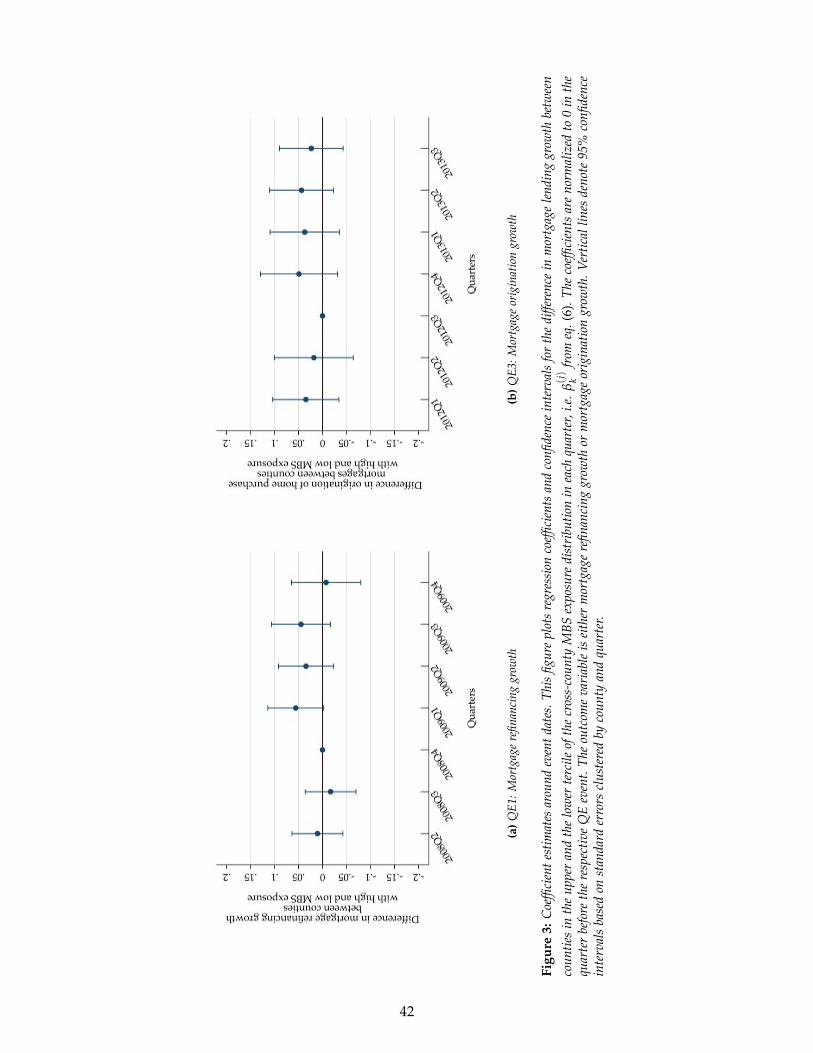
(a)

QE1

:Mor

tgag

ere

finan

cing

grow

th(b

)Q

E3:M

ortg

age

orig

inat

ion

grow

th

Figu

re3:

Coe

ffici

ente

stim

ates

arou

ndev

entd

ates

.Thi

sfig

ure

plot

sre

gres

sion

coef

ficie

nts

and

confi

denc

ein

terv

als

for

the

diffe

renc

ein

mor

tgag

ele

ndin

ggr

owth

betw

een

coun

ties

inth

eup

per

and

the

low

erte

rcile

ofth

ecr

oss-

coun

tyM

BSex

posu

redi

stri

butio

nin

each

quar

ter,

i.e.

β(j)

kfr

omeq

.(6)

.The

coef

ficie

nts

are

norm

aliz

edto

0in

the

quar

ter

befo

reth

ere

spec

tive

QE

even

t.Th

eou

tcom

eva

riab

leis

eith

erm

ortg

age

refin

anci

nggr

owth

orm

ortg

age

orig

inat

ion

grow

th.V

ertic

allin

esde

note

95%

confi

denc

ein

terv

als

base

don

stan

dard

erro

rscl

uste

red

byco

unty

and

quar

ter.

42

Figure 4: Employment growth between 2008 and 2015. Annual employment growth rate, ∆Empct, averaged separately overcounties in the upper and in the lower terciles of the cross-county MBS exposure distribution prior to QE3. The two verticallines indicate the quarters of the implementation of QE1 and QE3, respectively.

43

(a)

QE1

(b)

QE3

Figu

re5:

Coe

ffici

ente

stim

ates

arou

ndev

entd

ates

.Thi

sfig

ure

plot

sre

gres

sion

coef

ficie

nts

and

confi

denc

ein

terv

als

for

the

diffe

renc

ein

empl

oym

entg

row

thbe

twee

nco

untie

sin

the

uppe

ran

dth

elo

wer

terc

ileof

the

cros

s-co

unty

MBS

expo

sure

dist

ribu

tion

inea

chqu

arte

r,i.e

.β(j)

kfr

omeq

.(6)

.The

coef

ficie

nts

are

norm

aliz

edto

0in

the

quar

ter

befo

reth

ere

spec

tive

QE

even

t.V

ertic

allin

esde

note

95%

confi

denc

ein

terv

als

base

don

stan

dard

erro

rscl

uste

red

byco

unty

and

quar

ter.

44

(a)

QE1

(b)

QE3

Figu

re6:

Coe

ffici

ente

stim

ates

arou

ndev

entd

ates

.Thi

sfig

ure

plot

sre

gres

sion

coef

ficie

nts

and

confi

denc

ein

terv

als

for

the

diffe

renc

ein

car

regi

stra

tion

grow

thbe

twee

nco

untie

sin

the

uppe

ran

dth

elo

wer

terc

ileof

the

cros

s-co

unty

MBS

expo

sure

dist

ribu

tion

inea

chqu

arte

r,i.e

.β(j)

kfr

omeq

.(6)

.The

coef

ficie

nts

are

norm

aliz

edto

0in

the

quar

ter

befo

reth

ere

spec

tive

QE

even

t.V

ertic

allin

esde

note

95%

confi

denc

ein

terv

als

base

don

stan

dard

erro

rscl

uste

red

byco

unty

and

quar

ter.

45

Tables

Table 1: The announcement effect of QE1 (25 November 2008) and QE3 (13 September 2012)

Dependent variable: Daily return Daily risk-adjusted Return

(1) (2) (3) (4) (5) (6) (7) (8)( MBSTotAssets

)(1)b 0.069** 0.081** 0.055* 0.078*

(0.033) (0.041) (0.033) (0.042)( MBSTotAssets

)(3)b 0.019** 0.032*** 0.014 0.025**

(0.009) (0.012) (0.008) (0.011)log(Assets) 0.003 0.003*** 0.002 0.002**

(0.003) (0.001) (0.003) (0.001)Equity/Assets 0.164 0.081*** 0.080 0.076**

(0.139) (0.030) (0.139) (0.030)Profitability 0.071 -0.127 0.111 -0.105

(0.125) (0.082) (0.130) (0.085)Real Estate Ratio -0.017 -0.007 -0.003 -0.007

(0.038) (0.009) (0.038) (0.008)

R2a 0.012 0.049 0.012 0.115 0.008 0.035 0.007 0.066

N 325 325 315 315 325 325 315 315

Controls No Yes No Yes No Yes No Yes

This table studies the impact of MBS exposure on stock returns on QE announcement days. The tablereports coefficients from a cross-sectional regression of banks’ daily stock returns on bank characteristicson either November 25, 2008 (QE1) or on September 13, 2012 (QE3). The outcome variable is either thebank holding company-level raw daily return or the risk-adjusted return that controls for the marketreturn using a one-factor model, see eq. (1) and section 3.1.2 for details. Standard errors allow forheteroskedasticity. Stars indicate significance at the 10%, 5% and 1% levels, respectively.

46

Table 2: Counties with high and low MBS exposure

Low MBS exposure High MBS exposure Difference

Mean Std Mean Std Diff t-stat

Population (in thousand) 40.611 186.277 134.527 364.124 135.311 8.364Median Income 41035.527 9181.616 44032.547 10519.178 4228.495 9.000HousingMoodys 97.755 46.440 124.612 64.390 34.980 12.513∆Population2007Q4:2008Q4 0.001 0.010 0.005 0.010 0.004 8.058∆Housing2007Q4:2008Q4 -0.042 0.049 -0.041 0.047 0.000 0.125∆Income2007Q4:2008Q4 -0.027 0.053 -0.030 0.051 -0.001 -0.450

This table compares county characteristics prior to QE1 for counties in the upper and in the lower tercile of thecross-country MBS exposure distribution. MBS exposure is measured as the weighted average of bank-specific MBSratios averaged over the four quarters prior to QE1, with weights given by banks’ deposit shares per country, seeeq. (2).

47

Table 3: QE and county-level mortgage lending

Panel A: Mortgage refinancing

Dependent variable: %∆Refinancing

(1) (2) (3) (4) (5) (6) (7) (8)

QE(1)t × Exposure(1)HMDA

c 0.337** 0.327**(0.144) (0.144)

QE(1)t × Treat(1)HMDA

c 0.031*** 0.030***(0.011) (0.011)


c 0.048 0.060(0.147) (0.147)


c -0.010 -0.009(0.010) (0.010)

R2 0.593 0.593 0.563 0.563 0.189 0.189 0.174 0.174No. Counties 2854 2854 1899 1899 2855 2855 1922 1922N 19065 19065 12637 12637 19505 19505 13112 13112

Panel B: Mortgage origination

Dependent variable %∆Origination

(1) (2) (3) (4) (5) (6) (7) (8)


c -0.149 -0.159(0.156) (0.157)


c -0.019 -0.020(0.012) (0.012)


c 0.219 0.228(0.160) (0.161)


c 0.026** 0.027**(0.012) (0.012)

R2 0.239 0.239 0.220 0.220 0.213 0.213 0.192 0.192No. Counties 2804 2804 1865 1865 2807 2807 1896 1896N 19047 19047 12597 12597 19109 19109 12882 12882

County FE Yes Yes Yes Yes Yes Yes Yes YesTime FE Yes Yes Yes Yes Yes Yes Yes YesControls Yes Yes Yes Yes Yes Yes Yes YesInteracted Controls No Yes No Yes No Yes No Yes

This table reports estimates of the effect of MBS exposure on mortgage lending. The outcome variable iscounty-level quarterly growth of mortgage refinancing volume in panel A, and county-level quarterly growthin mortgage origination volume in panel B. MBS exposure is measured as banks’ MBS-to-asset ratios, weightedby banks’ average mortgage origination volume in a county in the four quarters prior to each QE event. Allspecifications include county and time fixed effects and county-level controls, see Equation (3) and Equation (4)for details. Column (1)-(2) and (5)-(6) report coefficients for the continuous treatment variable and column (3)-(4)and (7)-(8) report coefficients for the indicator treatment variable. Standard errors in parentheses are clustered bycounty and time. Stars indicate significance at the 10%, 5% and 1% levels, respectively.

48

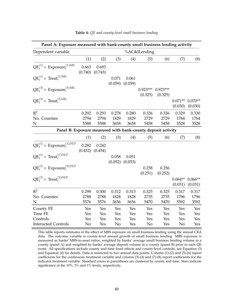
Table 4: QE and county-level small business lending

Panel A: Exposure measured with bank-county small business lending activity

Dependent variable %∆C&ILending

(1) (2) (3) (4) (5) (6) (7) (8)

QE(1)t × Exposure(1)SBL

c 0.663 0.693(0.740) (0.743)

QE(1)t × Treat(1)SBL

c 0.071 0.061(0.059) (0.059)


c 0.923*** 0.923***(0.325) (0.325)


c 0.071** 0.070**(0.030) (0.030)

R2 0.292 0.293 0.278 0.280 0.326 0.326 0.329 0.330No. Counties 2794 2794 1829 1829 2729 2729 1764 1764N 5588 5588 3658 3658 5458 5458 3528 3528

Panel B: Exposure measured with bank-county deposit activity

(1) (2) (3) (4) (5) (6) (7) (8)

QE(1)t × Exposure(1)DEP

c 0.282 0.242(0.452) (0.454)

QE(1)t × Treat(1)DEP

c 0.058 0.051(0.052) (0.053)


c 0.258 0.256(0.251) (0.252)


c 0.064** 0.066**(0.031) (0.031)

R2 0.298 0.300 0.312 0.313 0.325 0.325 0.317 0.317No. Counties 2788 2788 1828 1828 2735 2735 1796 1796N 5576 5576 3656 3656 5470 5470 3592 3592


This table reports estimates of the effect of MBS exposure on small business lending using the annual CRAdata. The outcome variable is county-level annual growth of small business lending. MBS exposure ismeasured as banks’ MBS-to-asset ratios, weighted by banks’ average small business lending volume in acounty (panel A) and weighted by banks’ average deposit volume in a county (panel B) prior to each QEevent. All specifications include county and time fixed effects and county-level controls, see Equation (3)and Equation (4) for details. Data is restricted to two annual data points. Column (1)-(2) and (5)-(6) reportcoefficients for the continuous treatment variable and column (3)-(4) and (7)-(8) report coefficients for theindicator treatment variable. Standard errors in parentheses are clustered by county and time. Stars indicatesignificance at the 10%, 5% and 1% levels, respectively.

49

Table 5: QE and county-level employment


Dependent variable ∆Emp

(1) (2) (3) (4) (5) (6) (7) (8)


c 0.017 0.026(0.023) (0.024)


c 0.001 0.002(0.002) (0.002)


c 0.051** 0.050**(0.020) (0.020)


c 0.004** 0.004**(0.002) (0.002)

R2 0.624 0.626 0.613 0.615 0.483 0.483 0.479 0.479No. Counties 2947 2947 1964 1964 2947 2947 1964 1964N 20205 20205 13436 13436 20293 20293 13478 13478


(1) (2) (3) (4) (5) (6) (7) (8)


c -0.036 -0.031(0.023) (0.023)


c -0.003* -0.002(0.001) (0.001)


c 0.014 0.013(0.018) (0.018)


c 0.003*** 0.003***(0.001) (0.001)

R2 0.599 0.600 0.588 0.589 0.501 0.501 0.507 0.507No. Counties 2946 2946 1965 1965 2952 2952 1968 1968N 20597 20597 13730 13730 20636 20636 13741 13741

Continued on next page

50

Table 5: (continued)

Panel C: Exposure measured with bank-county mortgage lending activity

(1) (2) (3) (4) (5) (6) (7) (8)


c 0.012 0.025(0.031) (0.031)


c 0.002 0.003(0.002) (0.002)


c 0.059** 0.060**(0.026) (0.026)


c 0.005*** 0.005***(0.002) (0.002)

R2 0.605 0.607 0.590 0.592 0.485 0.485 0.488 0.488No. Counties 2954 2954 1972 1972 2945 2945 1966 1966N 20204 20204 13457 13457 20284 20284 13505 13505


This table reports estimates of the effect of MBS exposure on employment. The outcome variable is county-level quarterly growth of employment. MBS exposure is measured as banks’ MBS-to-asset ratios, weighted bybanks’ average small business lending volume in a county (panel A), weighted by banks’ average depositvolume in a county (panel B) and weighted by banks’ average mortgage origination volume (panel C) priorto each QE event. All specifications include county and time fixed effects and county-level controls, seeEquation (3) and Equation (4) for details. Column (1)-(2) and (5)-(6) report coefficients for the continuoustreatment variable and column (3)-(4) and (7)-(8) report coefficients for the indicator treatment variable.Standard errors in parentheses are clustered by county and quarter. Stars indicate significance at the 10%, 5%and 1% levels, respectively.

51

Table 6: QE and county-level employment: Industry effects

Panel A: Employment in tradable/other and nontradable goods sector

Dependent variable ∆EmpTradOther ∆EmpNonTrad ∆EmpTradOther ∆EmpNonTrad

(1) (2) (3) (4) (5) (6) (7) (8)


c -0.026 0.218**(0.072) (0.089)


c -0.005 0.016**(0.006) (0.006)


c 0.095* -0.001(0.056) (0.043)


c 0.014** 0.005(0.006) (0.005)

R2 0.476 0.484 0.440 0.427 0.475 0.490 0.425 0.425No. Counties 2959 1970 2959 1970 2951 1964 2951 1964N 5918 3940 5918 3940 5902 3928 5902 3928

Panel B: Employment by financial dependence of industry

Dependent variable ∆EmpFin ∆EmpNonFin ∆EmpFin ∆EmpNonFin

(1) (2) (3) (4) (5) (6) (7) (8)


c 0.015 -0.098(0.125) (0.106)


c 0.003 -0.011(0.010) (0.008)


c 0.116 0.066(0.089) (0.076)


c 0.013 0.006(0.008) (0.008)

R2 0.435 0.430 0.478 0.473 0.454 0.463 0.424 0.426No. Counties 2959 1970 2959 1970 2960 1973 2960 1973N 5918 3940 5918 3940 5920 3946 5920 3946

County FE Yes Yes Yes Yes Yes Yes Yes YesTime FE Yes Yes Yes Yes Yes Yes Yes YesControls Yes Yes Yes Yes Yes Yes Yes Yes

This table reports estimates of the effect of MBS exposure on employment by industry splits using the annualQCEW data. In panel A, the outcome variable is county-level annual employment growth by tradable ornon-tradable industry. We use the definition of non-tradable industries of Mian and Sufi (2014). In panelB, the outcome variable is county-level annual employment growth by industry’s financial dependence. Wemeasure financial dependence as in Almeida et al. (2010). MBS exposure is measured as banks’ MBS-to-assetratios, weighted by banks’ average small business lending volume in a county prior to each QE event. Allspecifications include county and time fixed effects and county-level controls, interacted with QE event dummies,see Equation (3) and Equation (4) for details. Data is restricted to two annual data points. Column (1)-(2) and(5)-(6) report coefficients for the continuous treatment variable and column (3)-(4) and (7)-(8) report coefficientsfor the indicator treatment variable. Standard errors in parentheses are clustered by county and time. Starsindicate significance at the 10%, 5% and 1% levels, respectively.

52

Table 7: QE and county-level auto purchases

Exposure measured with bank-county mortgage lending activity

Dependent variable ∆Auto

(1) (2) (3) (4) (5) (6) (7) (8)


c 0.505*** 0.471***(0.105) (0.107)


c 0.036*** 0.035***(0.009) (0.009)


c 0.054 0.057(0.087) (0.088)


c 0.014* 0.013*(0.007) (0.007)

R2 0.551 0.551 0.529 0.530 0.206 0.206 0.200 0.200No. Counties 2683 2683 1794 1794 2685 2685 1795 1795N 18775 18775 12544 12544 18790 18790 12560 12560


This table reports estimates of the effect of MBS exposure on auto purchases. The outcome variable is county-levelquarterly growth of car registrations. MBS exposure is measured as banks’ MBS-to-asset ratios, weighted by banks’average mortgage origination volume prior to each QE event. All specifications include county and time fixedeffects and county-level controls, see Equation (3) and Equation (4) for details. Column (1)-(2) and (5)-(6) reportcoefficients for the continuous treatment variable and column (3)-(4) and (7)-(8) report coefficients for the indicatortreatment variable. Standard errors in parentheses are clustered by county and time. Stars indicate significance atthe 10%, 5% and 1% levels, respectively.

53

Table 8: QE and bank-firm-level lending

Panel A: Continuous treatment

Dependent variable ∆C&I lending

Sample Entire sample Not in Compustat Compustat

(1) (2) (3) (4) (5) (6)

QE(3) ×( MBS

TotAssets

)(3)b 0.319*** 0.354*** 0.326** 0.424*** 0.151*** 0.130**

(0.021) (0.052) (0.119) (0.074) (0.053) (0.054)

R2 0.207 0.528 0.213 0.559 0.174 0.486No Banks 25 25 25 25 25 25No Firms 127305 9768 124729 8005 2638 1779No Bank-Firm-Relationships 152803 33642 141636 23349 11231 10318No obs 641048 145669 587074 96160 53696 49288

Panel B: Binary treatment



(1) (2) (3) (4) (5) (6)

QE(3)× Treat(3)b 0.025*** 0.030*** 0.024*** 0.031*** 0.021*** 0.017***(0.002) (0.004) (0.007) (0.006) (0.005) (0.005)


Bank-Firm FE Yes Yes Yes Yes Yes YesTime FE Yes No Yes No Yes NoBank Controls Yes Yes Yes Yes Yes YesInteracted Bank Controls Yes Yes Yes Yes Yes YesFirm-Time FE No Yes No Yes No Yes

This table reports estimates of the effect of banks’ MBS exposure on bank-firm-level lending. The outcomevariable is growth of total lending from each bank to each firm. MBS exposure is a bank’s average MBS-to-assets ratio in the four quarters prior to QE3. All specifications include bank-firm fixed effects and bank-levelcontrols. Specifications include either time fixed effects or firm-time fixed effects, see eq. (7) for details. Weuse the computationally efficient estimator of linear models with multiple high-dimensional fixed effectsproposed by Correia (2017). Exposure is continuous in panel A and binary in panel B, i.e. in panel B,treatment is equal to 1 if a bank’s MBS exposure is above the median of the cross-bank MBS exposuredistribution. In columns (1) and (2), the data consist of all bank-firm relationships identified in the Y14 data.Columns (3) and (4) report estimates for firms within the Y14 data that cannot be matched to Compustat,and columns (5) and (6) report estimates that can be matched to Compustat. Standard errors in parenthesesare clustered at the firm-time level and stars indicate significance at the 10%, 5%, and 1% level, respectively.

54

Table 9: QE and firm-level lending, investment and employment

Panel A: Firm-level borrowing

Dependent variable ∆Credit

Sample Compustat Not in Compustat

(1) (2) (3) (4) (5) (6) (7) (8)

Exposure(3)i 0.255 0.334* 0.190*** 0.203***(0.158) (0.201) (0.036) (0.040)

Treat(3)i 0.012* 0.013* 0.017*** 0.017***(0.006) (0.008) (0.002) (0.003)

R2 .0014 .0028 .0045 .0097 .00048 .0018 .00067 .0021No Firms 1852 1171 1493 919 40319 27576 33623 23067

Panel B: Firm-level investment

Dependent variable ∆Investment (in ppt)

Sample Compustat Not in Compustat

(1) (2) (3) (4) (5) (6) (7) (8)

Exposure(3)i 3.628** 1.641 13.461*** 12.599***(1.703) (1.910) (0.846) (0.832)

Treat(3)i 0.141** 0.075 0.431*** 0.217***(0.071) (0.082) (0.046) (0.047)

R2 .0021 .0033 .014 .015 .0068 .003 .0096 .047No Firms 1852 1171 1690 1050 40319 27576 33623 23067

Panel C: Firm-level employment

Dependent variable ∆Emp2012Q4:2013Q4 ∆Emp2012Q4:2014Q4

Sample Compustat

(1) (2) (3) (4) (5) (6) (7) (8)

Exposure(3)i 0.458** 0.431** 0.640** 0.665**(0.180) (0.200) (0.273) (0.290)

Treat(3)i 0.010* 0.011* 0.011 0.016*(0.006) (0.006) (0.009) (0.010)

R2 .014 .01 .02 .018 .029 .026 .064 .067No Firms 1894 1256 1578 1045 1775 1173 1466 970

Firm Controls No No Yes Yes No No Yes Yes

This table reports estimates of the effect of firms’ MBS exposure (via relationships to exposed banks) on lending,investment and employment. The outcome variable is a firm’s lending growth between 2012Q4 and 2013Q4 in panelA, the difference in capital expenditure between 2012Q4 to 2013Q4 over assets in 2012Q4 in panel B, and employmentgrowth from 2012Q to 2013Q4 or from from 2012Q to 2014Q4 in panel C. Exposure is measured as banks’ MBS-to-assetratios averaged over four quarters prior to QE3, weighted by lending volume at the bank-firm level averaged over fourquarters prior to QE3, see eq. (9) for details. Panels A and B report estimates for firms in the Y14 data that can bematched to Compustat in columns (1) to (4), and estimates for firms that cannot be matched to Compustat in columns (5)to (8). Panel C uses only firms that can be matched to Compustat because employment is not available in the Y14 data.Firm controls include the firms’s leverage, z-Score, current income, and size measured as log of total assets, see eq. (11)for details. Robust standard errors in parentheses. Stars indicate significance at the 10%, 5%, and 1% level, respectively.

55

Table 10: QE and county-bank level mortgage lending


Dependent variable ∆Refinancing (conforming) ∆Refinancing (non-conforming)

(1) (2) (3) (4) (5) (6) (7) (8)

QE(1)t ×

( MBSAssets

)(1)b 0.740*** 0.182** 0.863*** 0.659**

(0.060) (0.071) (0.243) (0.304)

QE(3)t ×

( MBSAssets

)(3)b 0.091 0.087 0.099 0.141

(0.087) (0.110) (0.186) (0.199)

R2 .14 .26 .037 .14 .05 .28 .016 .18N 173910 172138 217239 212450 25565 21781 46110 42604No Banks 3078 3075 2757 2738 1923 1638 1776 1595No Counties 3078 2910 3070 2910 1852 1009 1932 1172


Dependent variable ∆Origination (conforming) ∆Origination (non-conforming)

(1) (2) (3) (4) (5) (6) (7) (8)

QE(1)t ×

( MBSAssets

)(1)b 0.108 0.104 0.561 0.212

(0.126) (0.140) (0.485) (0.553)

QE(3)t ×

( MBSAssets

)(3)b 0.100 0.113 0.486*** 0.627***

(0.068) (0.077) (0.169) (0.199)

R2 .055 .18 .034 .16 .18 .36 .042 .23N 190282 187973 224625 216700 26843 23828 38568 35318No Banks 3330 3330 3004 3000 1698 1502 1504 1315No Counties 3083 2909 3070 2867 1501 881 1515 872

Bank-County FE Yes Yes Yes Yes Yes Yes Yes YesTime FE Yes No Yes No Yes No Yes NoBank Controls Yes Yes Yes Yes Yes Yes Yes YesInteracted Bank Controls Yes Yes Yes Yes Yes Yes Yes YesCounty-Time FE No Yes No Yes No Yes No Yes

This table reports estimates of the effect of MBS exposure on county-bank level mortgage lending. The outcomevariable is county-bank level mortgage refinancing growth for conforming and non-conforming mortgages in panelA, and county-bank level mortgage origination growth for conforming and non-conforming mortgages in panel B. Allspecifications include bank-county fixed effects and bank-level controls. Specifications include either time fixed effects orcounty-time fixed effects, see eq. (12) for details. We use the computationally efficient estimator of linear models withmultiple high-dimensional fixed effects proposed by Correia (2017). Standard errors are two-way clustered at the countyand time levels. Stars indicate significance at the 10%, 5% and 1% levels, respectively.

56

Table 11: Robustness: QE2, Tapering and mortgage lending


Dependent variable: ∆Refinancing

(1) (2) (3) (4) (5) (6) (7) (8)


c 0.045 0.082(0.156) (0.155)


c -0.006 -0.000(0.011) (0.011)

Tapert × Exposure(3)HMDAc -0.228 -0.229

(0.174) (0.175)Tapert × Treat(3)HMDA

c -0.029*** -0.029***(0.011) (0.011)

R2 0.382 0.383 0.348 0.349 0.219 0.219 0.198 0.198No. Counties 2869 2869 1907 1907 2860 2860 1906 1906N 19762 19762 13081 13081 19679 19679 13054 13054


Dependent variable ∆Origination

(1) (2) (3) (4) (5) (6) (7) (8)


c 0.068 0.045(0.174) (0.184)


c -0.014 -0.018(0.013) (0.014)



c -0.020 -0.030*(0.016) (0.017)

R2 0.257 0.257 0.246 0.246 0.333 0.334 0.300 0.301No. Counties 2847 2847 1893 1893 2856 2856 1927 1927N 19311 19311 12794 12794 19502 19502 13138 13138


This table reports estimates of MBS exposure on mortgage lending. The outcome variable is county-level quarterlygrowth of mortgage refinancing volume in panel A, and county-level quarterly growth in mortgage originationvolume in panel B. MBS exposure is measured as banks’ MBS-to-asset ratios, weighted by banks’ average mortgageorigination volume in a county in the four quarters prior to either QE2 or Tapering. All specifications includecounty and time fixed effects and county-level controls, see Equation (3) and Equation (4) for details. Column(1)-(2) and (5)-(6) report coefficients for the continuous treatment variable and column (3)-(4) and (7)-(8) reportcoefficients for the indicator treatment variable. Standard errors in parentheses are clustered by county and time.Stars indicate significance at the 10%, 5% and 1% levels, respectively.

57

Table 12: Robustness: QE2, Tapering and employment



(1) (2) (3) (4) (5) (6) (7) (8)


c 0.006 0.000(0.012) (0.012)


c 0.000 -0.000(0.001) (0.001)

Tapert × Exposure(3)SBLc -0.028** -0.023*

(0.013) (0.013)Tapert × Treat(3)SBL

c -0.002** -0.002*(0.001) (0.001)

R2 0.547 0.549 0.527 0.529 0.527 0.527 0.527 0.527No. Counties 2947 2947 1967 1967 2950 2950 1967 1967N 20278 20278 13494 13494 20335 20335 13549 13549


(1) (2) (3) (4) (5) (6) (7) (8)


c 0.012 0.013(0.009) (0.009)


c 0.001 0.001(0.001) (0.001)

Tapert × Exposure(3)DEPc -0.031 -0.032

(0.026) (0.026)Tapert × Treat(3)DEP

c -0.005 -0.005(0.004) (0.004)

R2 0.521 0.521 0.512 0.512 0.370 0.370 0.345 0.345No. Counties 2929 2929 1949 1949 2946 2946 1966 1966N 20225 20225 13422 13422 20608 20608 13743 13743

Continued on next page

58

Table 12: (continued)

Panel C: Exposure measured with bank-county mortgage lending activity

(1) (2) (3) (4) (5) (6) (7) (8)


c 0.043 0.010(0.035) (0.035)


c 0.004* 0.002(0.002) (0.003)



c -0.003 -0.003(0.002) (0.003)

R2 0.539 0.540 0.529 0.530 0.516 0.517 0.478 0.478No. Counties 2900 2900 1974 1974 2945 2945 1965 1965N 20279 20279 13797 13797 20493 20493 13661 13661


This table reports estimates of MBS exposure on employment. The outcome variable is county-level quarterlygrowth of employment. MBS exposure is measured as banks’ MBS-to-asset ratios, weighted by banks’ averagesmall business lending volume in a county (panel A), weighted by banks’ average deposit volume in a county(panel B) and weighted by banks’ average mortgage origination volume (panel C) prior to each QE event. Allspecifications include county and time fixed effects and county-level controls, see Equation (3) and Equation (4)for details. Column (1)-(2) and (5)-(6) report coefficients for the continuous treatment variable and column(3)-(4) and (7)-(8) report coefficients for the indicator treatment variable. Standard errors in parentheses areclustered by county and time. Stars indicate significance at the 10%, 5% and 1% levels, respectively.

59

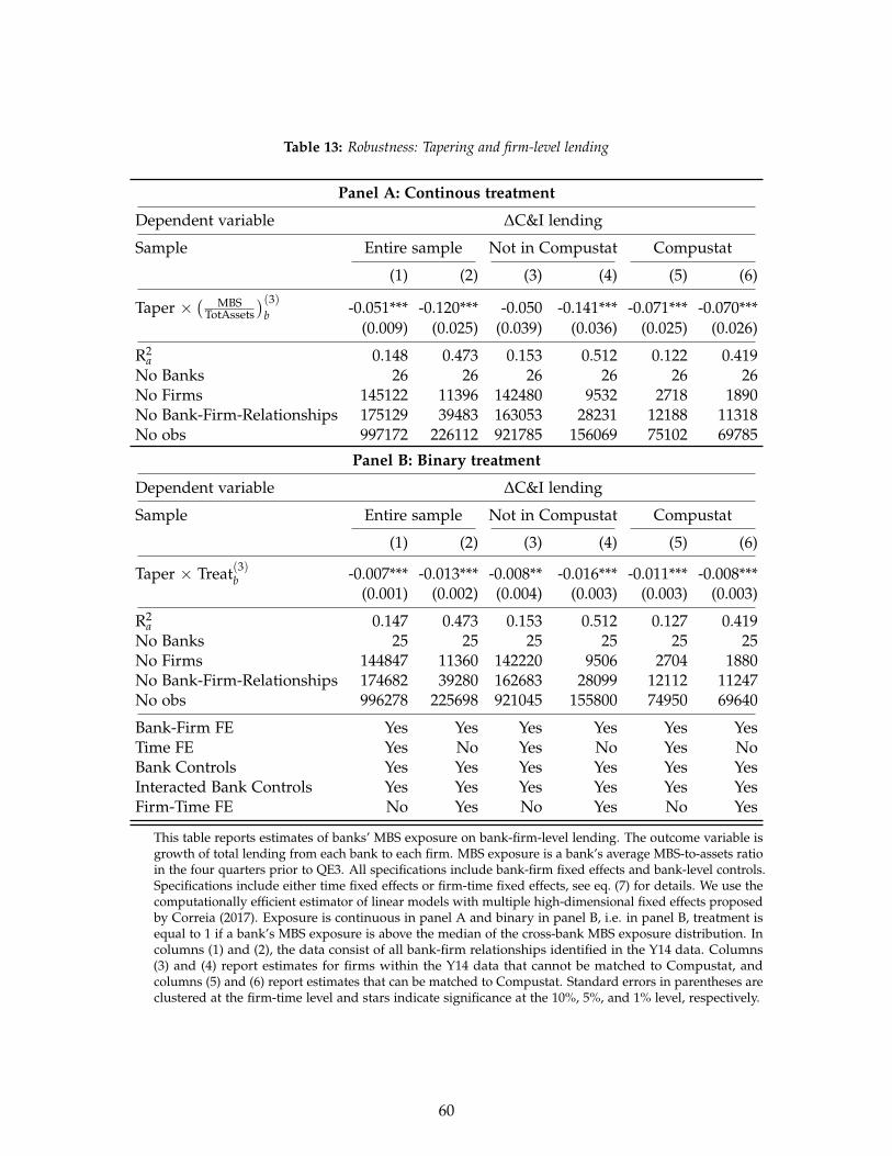
Table 13: Robustness: Tapering and firm-level lending

Panel A: Continous treatment



(1) (2) (3) (4) (5) (6)

Taper ×( MBS

TotAssets

)(3)b -0.051*** -0.120*** -0.050 -0.141*** -0.071*** -0.070***

(0.009) (0.025) (0.039) (0.036) (0.025) (0.026)

R2a 0.148 0.473 0.153 0.512 0.122 0.419

No Banks 26 26 26 26 26 26No Firms 145122 11396 142480 9532 2718 1890No Bank-Firm-Relationships 175129 39483 163053 28231 12188 11318No obs 997172 226112 921785 156069 75102 69785




(1) (2) (3) (4) (5) (6)

Taper × Treat(3)b -0.007*** -0.013*** -0.008** -0.016*** -0.011*** -0.008***(0.001) (0.002) (0.004) (0.003) (0.003) (0.003)

R2a 0.147 0.473 0.153 0.512 0.127 0.419

No Banks 25 25 25 25 25 25No Firms 144847 11360 142220 9506 2704 1880No Bank-Firm-Relationships 174682 39280 162683 28099 12112 11247No obs 996278 225698 921045 155800 74950 69640

Bank-Firm FE Yes Yes Yes Yes Yes YesTime FE Yes No Yes No Yes NoBank Controls Yes Yes Yes Yes Yes YesInteracted Bank Controls Yes Yes Yes Yes Yes YesFirm-Time FE No Yes No Yes No Yes

This table reports estimates of banks’ MBS exposure on bank-firm-level lending. The outcome variable isgrowth of total lending from each bank to each firm. MBS exposure is a bank’s average MBS-to-assets ratioin the four quarters prior to QE3. All specifications include bank-firm fixed effects and bank-level controls.Specifications include either time fixed effects or firm-time fixed effects, see eq. (7) for details. We use thecomputationally efficient estimator of linear models with multiple high-dimensional fixed effects proposedby Correia (2017). Exposure is continuous in panel A and binary in panel B, i.e. in panel B, treatment isequal to 1 if a bank’s MBS exposure is above the median of the cross-bank MBS exposure distribution. Incolumns (1) and (2), the data consist of all bank-firm relationships identified in the Y14 data. Columns(3) and (4) report estimates for firms within the Y14 data that cannot be matched to Compustat, andcolumns (5) and (6) report estimates that can be matched to Compustat. Standard errors in parentheses areclustered at the firm-time level and stars indicate significance at the 10%, 5%, and 1% level, respectively.

60

Description of appendices

• Appendix A: Bank-level analysis of QE and mortgage and small business lending

• Appendix B: Supplementary figures

• Appendix C: Supplementary tables

• Appendix D: Variable construction

61

Appendix A Bank-level analysis

A.1 Empirical Strategy

This section provides detailed bank-level results complementary to those of previous studies. We

construct our bank-level exposure measure as a bank’s MBS scaled by total assets. Figure B.1 shows the

distribution of the exposure measure averaged over the four quarters prior to QE1. More than a quarter

of all commercial banks held no MBS at all, and the average MBS-to-asset ratio was around 12% in the

upper quartile of the cross-sectional distribution across banks.

[FIGURE B.1 ABOUT HERE]

While banks with higher MBS shares tend to be larger and tend to operate with higher leverage

than banks with relatively lower MBS shares, banks sorted by MBS shares are otherwise very similar in

other observable characteristics. Table C.5 gives a sense of those differences, splitting the sample of all

commercial banks in the United States by the median of the average MBS share in the 4 quarters prior

to QE1.

[TABLES C.5 and C.6 ABOUT HERE]

In order to assess the effect of the Fed’s actions at the bank level, we employ a difference-in-

differences (DiD) design with a continuous treatment variable. The unit of observation is the commercial

bank and the main specification is given by:

ln(ybt) = α + β

(MBS

Total Assets

)(j)

bQE(j)

t + θXbt + γb + τt + εbt (13)

Here, yb,t is the amount of lending of bank b at time t. We use different categories of lending in our

regressions, including total lending, mortgage lending, and C&I lending. Moreover, we distinguish

between newly originated and refinanced mortgages as well as between small business loans of different

sizes. We estimate the regression for each episode of quantitative easing, j = 1, 2, 3, with a time window

of four quarters before and after the introduction of the respective program.11 QE(j)t is an indicator

variable equal to 1 after the introduction of the j-th round of quantitative easing.12 We measure bank b’s

11All results are robust to changing the time window as well as to pooling events in a single regression.12Given that the data on the commercial bank level is quarterly, we choose 2009Q1 as the event date for QE1, and 2010Q4

62

MBS-to-assets ratio,( MBS

Total Assets

)(j)b , as the average ratio over the 4 quarters prior to the j-th round of QE.

Additionally, our regression includes bank-fixed effects, γb, and time-fixed effects, τt, to control

for fixed differences between banks and for differences over time that affect all banks. We include

bank-specific time-varying controls Xbt to control for remaining differences between banks. Controls

included in the regression are listed in Table C.6.

A.2 Results

Table C.8 estimates Equation (13) for three different dependent variables: the natural logarithm of the

overall amount of lending, of the amount of mortgage lending, and of the amount of C&I lending.

[TABLE C.8 ABOUT HERE]

We make three observations about the results depicted in Table C.8. First, for total lending volume,

the interaction term between QE and a bank’s MBS-to-asset ratio prior to QE is positive and statistically

significant for QE1 and QE3. This suggests that banks with large MBS holdings issued relatively more

loans after QE1 and QE3. Second, focusing on real estate lending and C&I lending, we find that real

estate related lending increased more at affected banks after QE1 and QE3, while C&I lending increased

only after QE3. Third, there is no effect on lending during QE2. 13 Finally, the results are economically

sizable. For instance, moving a bank from the 25th percentile of the MBS distribution to the 75th

percentile implies an increase in C&I lending of about 1.3% after QE3. The overall pattern of our results

confirms the findings of Darmouni and Rodnyansky (2017) of a stimulating effects of QE1 and QE3 on

bank lending.

However, our analysis goes further. Using data collected under the HMDA and aggregated to the

bank-level, we provide further evidence on the effect on lending for residential housing. Importantly,

the (confidential) version of HMDA data that we use, allows us to estimate regressions at the quarterly

level (rather than the annual level which is the frequency in public HMDA data) to get a more precise

and 2012Q4 as the event dates for QE2 and QE3, respectively.13This is consistent with the focus of the different programs on MBS purchases (QE1, QE3) and U.S. Treasury purchases

(QE2). We should not expect QE2 to affect banks with high and low MBS shares differently via a narrow channel. Note thatbanks generally hold less Treasuries than MBS, and the price effect on Treasuries is generally weaker. Note also that loweringTreasury yields, as done by QE2, can yet affect bank lending: mortgage rates move with Treasury rates, and hence QE2 couldspur refinancing in the mortgage market. Indeed, the positive coefficient for overall lending and mortgage lending, Column(2) and Column (5), point to a weak effect on mortgage-related lending. However, the absence of a significant effect can berationalized by the high refinancing activity after QE1 and the relatively weaker effect on long-term rates of QE2 compared toQE1 (see Gilchrist et al. (2015)).

63

sense of the timing of effects. Table C.9 shows the estimates from Equation (13), but uses refinanced

mortgages as well as newly issued mortgages as dependent variables. Columns (1) and (2) confirm the

results for total real estate lending from the Call Report data in Table C.8. The additional specifications

distinguish between new origination of mortgages and refinancing of existing mortgages. Even though

aggregate lending related to housing increased during QE1 and QE3, the underlying type of lending

is different. In particular, results in columns (3) and (4) reveal that the effect during QE1 is driven by

increased refinancing activity of affected banks, consistent with the findings by Di Maggio et al. (2016),

who show that QE1 spurred refinancing activity in the mortgage market. Columns (5) and (6) show that

the effect of QE3 is driven by origination of mortgages for new home purchases and by refinancing of

existing mortgages.


Using additional data collected under the Community Reinvestment Act (CRA) on small business

lending, we estimate the main specification using four related types of small business lending as

dependent variables: loans to small business with face value of $ 0 to 100k, $ 100k to 250k, and $ 250k

to 1m, as well as loans to businesses with an annual revenue of less than $ 1 million. Table C.10 shows

results. Consistent with the results in Table C.8, small business lending does not respond in any category

after QE1 and estimated coefficients fluctuate widely (columns (1), (3), (5), and (7) of Table C.10). For

QE3, however, we find consistent effects across all categories (columns (2), (4), (6), and (8)): Coefficients

are only significant in two of the categories but are positive and of similar magnitude across all of three

of them. In particular, note that the coefficient for loans with a face value between 250k to 1m, the

category with the highest aggregate volume, is significant.


A bank that holds 12% of its assets in MBS instead of having no MBS holdings, increased the issuance

of small business loans with a face value between 250k and 1m by about 4% after QE3. The magnitude

is comparable to the magnitude of the effect on total C&I lending in Table C.8.

64

Appendix B Supplementary Figures

Figure B.1: Distribution of banks’ average MBS shares prior to QE1

65

(a)

Mor

tgag

ean

dsm

allb

usin

ess

lend

ing,

ρ=

0.49

(b)

Mor

tgag

ele

ndin

gan

dde

posi

ts,ρ

=0.

56(c

)Sm

all b

usin

ess

lend

ing

and

depo

sits

,ρ=

0.54

Figu

reB

.2:S

catt

erpl

otof

diffe

rent

expo

sure

mea

sure

spr

ior

toQ

E3.A

coun

ty’s

MBS

expo

sure

ism

easu

red

asba

nks’

MBS

-to-

asse

trat

ios,

wei

ghte

dby

bank

s’av

erag

esm

allb

usin

ess

lend

ing

volu

me

ina

coun

ty,w

eigh

ted

byba

nks’

aver

age

depo

sitv

olum

ein

aco

unty

(pan

elB)

and

wei

ghte

dby

bank

s’av

erag

em

ortg

age

orig

inat

ion

volu

me

(pan

elC

)pri

orto

each

QE

even

t.

66

Figure B.3: Employment growth between 2008 and 2014 in the annual CBP data. Annual employment growth rate, ∆Empct,averaged separately over counties in the upper and in the lower terciles of the cross-county MBS exposure distribution priorto QE3.

Figure B.4: Distribution of firms’ average total lending in 2012 in the Y-14 data by the number of bank-firm relationships.A firm and a bank have a relationship if the bank lends to the firm in at least three quarters between 2011Q3 and 2016Q2.

67

Appendix C Supplementary Tables

Table C.1: Banks with high and low MBS shares: Bank in Y14 data

Low MBS Share High MBS Share Difference


log(assets) 19.428 1.418 19.042 0.948 -0.339 -0.696Equity/TotalAssets 0.106 0.029 0.116 0.015 0.009 1.125Tier 1 Ratio 0.129 0.024 0.123 0.021 -0.005 -0.694RoA 0.009 0.012 0.005 0.009 -0.003 -1.165Real Estate Ratio 0.175 0.182 0.279 0.145 0.096 1.452Loans to Assets 0.469 0.262 0.560 0.214 0.083 0.862C&I Loan Ratio 0.317 0.321 0.231 0.091 -0.086 -0.929Non-performing Loans Ratio 0.010 0.010 0.012 0.009 0.001 0.505

This table reports bank characteristics prior to QE3 averaged separately for banks above and below themedian of the cross-bank MBS-to-assets distribution, for banks in the Y14 data only. MBS-to-assets areaveraged over the four quarters prior to QE3 for each bank.

Table C.2: Descriptive statistics for bank-level control variables: Banks in Y14 data

Mean Std 10th Perc 25th Perc Median 75th Perc 90th Perc N

MBS/TotalAssets 0.095 0.058 0.009 0.031 0.103 0.154 0.162 502MBS/TotalSecurities 0.553 0.293 0.195 0.236 0.578 0.806 0.907 502log(assets) 19.237 1.223 17.826 18.208 18.961 20.434 21.365 502Equity/TotalAssets 0.111 0.024 0.080 0.096 0.111 0.123 0.135 502Tier 1 Ratio 0.126 0.023 0.101 0.111 0.122 0.137 0.158 502RoA 0.007 0.012 -0.001 0.003 0.006 0.011 0.017 502Real Estate Ratio 0.227 0.173 0.002 0.029 0.225 0.369 0.468 502Loans to Assets 0.514 0.243 0.075 0.340 0.630 0.699 0.746 502C&I Loan Ratio 0.282 0.279 0.053 0.148 0.221 0.303 0.603 502Non-performing Loans Ratio 0.011 0.010 0.001 0.004 0.009 0.016 0.024 502

This table reports means, standard deviations and various percentiles of variables used as controls in bank-levelregressions. The dataset runs from 2011Q3 to 2016Q3 and includes 25 banks.

68

Table C.3: Descriptive statistics for firm-level variables


Sample CompustatTotal Assets (in million) 15005.26 108343.67 192.69 611.90 2019.86 6728.73 21728.00 1831Total Bank Credit 3823.87 7029.06 162.74 500.00 1819.39 4747.69 9231.01 1831Capital Expenditures 414.85 1449.08 1.13 10.18 51.92 234.46 904.52 1831No of Employees 16927.64 67383.27 238.00 999.00 3400.00 11800.00 35283.00 1831Sample Not in CompustatTotal Assets (in million) 1381.05 27442.46 1.57 4.94 16.05 71.55 421.42 40319Total Bank Credit 211.18 765.16 12.07 18.59 40.20 129.14 402.39 40319Capital Expenditures 30.29 1013.57 -0.17 0.00 0.01 1.17 11.94 40319

This table reports means, standard deviations and various percentiles of firm characteristics for firms in the Y14 datacollection. Panel A includes firms that can be matched to Compustat, and also includes employment which is not availablein the Y14 data. Panel B includes firms that cannot be matched to Compustat. Data are as reported in 2012Q4.

69

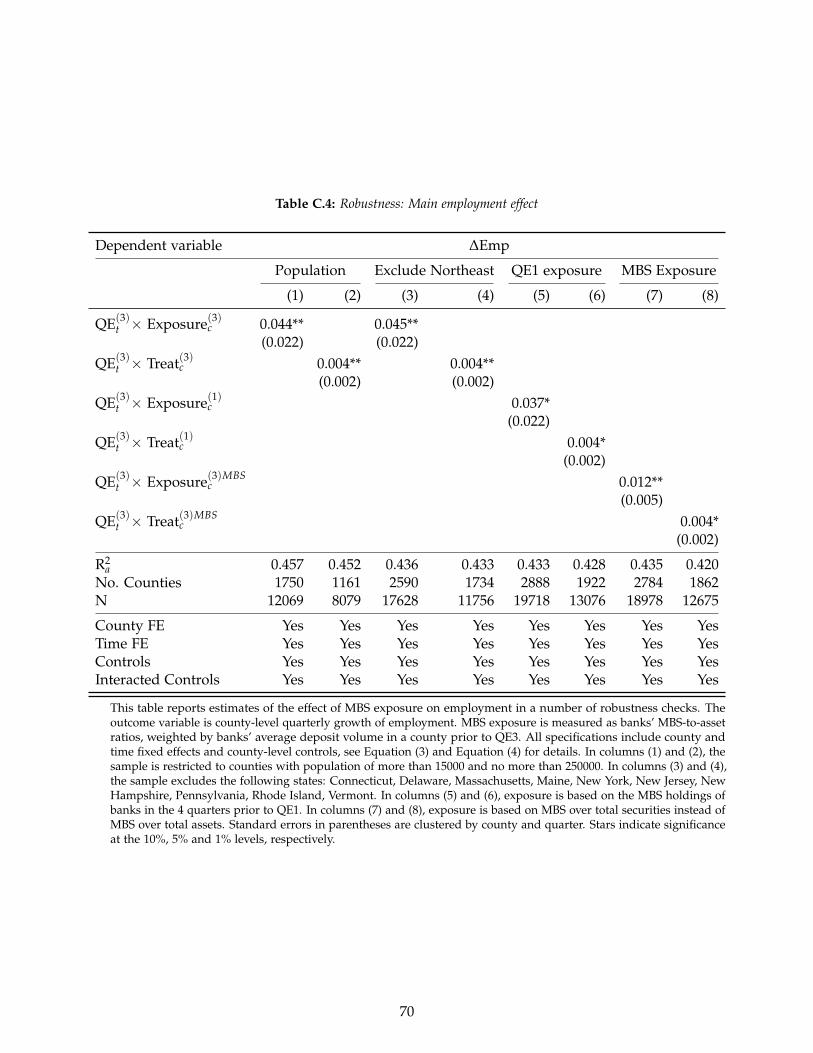
Table C.4: Robustness: Main employment effect


Population Exclude Northeast QE1 exposure MBS Exposure

(1) (2) (3) (4) (5) (6) (7) (8)

QE(3)t × Exposure(3)c 0.044** 0.045**

(0.022) (0.022)QE(3)

t × Treat(3)c 0.004** 0.004**(0.002) (0.002)

QE(3)t × Exposure(1)c 0.037*

(0.022)QE(3)

t × Treat(1)c 0.004*(0.002)

QE(3)t × Exposure(3)MBS

c 0.012**(0.005)

QE(3)t × Treat(3)MBS

c 0.004*(0.002)

R2a 0.457 0.452 0.436 0.433 0.433 0.428 0.435 0.420

No. Counties 1750 1161 2590 1734 2888 1922 2784 1862N 12069 8079 17628 11756 19718 13076 18978 12675

County FE Yes Yes Yes Yes Yes Yes Yes YesTime FE Yes Yes Yes Yes Yes Yes Yes YesControls Yes Yes Yes Yes Yes Yes Yes YesInteracted Controls Yes Yes Yes Yes Yes Yes Yes Yes

This table reports estimates of the effect of MBS exposure on employment in a number of robustness checks. Theoutcome variable is county-level quarterly growth of employment. MBS exposure is measured as banks’ MBS-to-assetratios, weighted by banks’ average deposit volume in a county prior to QE3. All specifications include county andtime fixed effects and county-level controls, see Equation (3) and Equation (4) for details. In columns (1) and (2), thesample is restricted to counties with population of more than 15000 and no more than 250000. In columns (3) and (4),the sample excludes the following states: Connecticut, Delaware, Massachusetts, Maine, New York, New Jersey, NewHampshire, Pennsylvania, Rhode Island, Vermont. In columns (5) and (6), exposure is based on the MBS holdings ofbanks in the 4 quarters prior to QE1. In columns (7) and (8), exposure is based on MBS over total securities instead ofMBS over total assets. Standard errors in parentheses are clustered by county and quarter. Stars indicate significanceat the 10%, 5% and 1% levels, respectively.

70

Table C.5: Banks with high and low MBS shares

Low MBS Share High MBS Share Difference


log(assets) 11.622 1.262 12.171 1.396 0.549 17.660Equity/TotalAssets 0.133 0.119 0.115 0.075 -0.018 -8.263Deposit Ratio 0.799 0.152 0.798 0.101 -0.001 -0.365Trading Book Ratio 0.001 0.013 0.001 0.006 -0.000 -0.245Profitability 0.006 0.183 0.003 0.015 -0.003 -1.598Overhead Ratio 0.820 1.225 0.807 1.129 -0.012 -0.612Net interest margin 0.020 0.685 0.023 0.011 0.003 0.451Non-performing Loans Ratio 0.010 0.018 0.010 0.017 -0.001 -1.480Delinquency Ratio 1.950 1.104 1.916 1.066 -0.034 -1.476Real Estate Ratio 0.676 0.180 0.693 0.163 0.016 4.080C&I Loan Ratio 0.154 0.114 0.155 0.099 0.002 0.698Tier 1 Ratio 0.233 1.116 0.173 0.350 -0.061 -3.360

This table reports bank characteristics prior to QE1 averaged separately for banks above and below themedian of the cross-bank MBS-to-assets distribution. MBS-to-assets are averaged over the four quartersprior to QE1 for each bank.

Table C.6: Descriptive statistics for bank-level control variables


Agency MBS/TotalAssets 0.08 0.10 0.00 0.00 0.05 0.12 0.21 166563Agency MBS/TotalSecurities 0.36 0.33 0.00 0.02 0.31 0.60 0.84 166563Treasuries/TotalAssets 0.01 0.03 0.00 0.00 0.00 0.00 0.01 166563Treasuries/TotalSecurities 0.03 0.13 0.00 0.00 0.00 0.00 0.04 166563log(Assets) 12.07 1.31 10.62 11.23 11.93 12.71 13.61 166563Equity/TotalAssets 0.11 0.04 0.08 0.09 0.10 0.12 0.15 166563Deposit Ratio 0.84 0.07 0.75 0.81 0.85 0.88 0.90 166563Trading Book Ratio 0.00 0.01 0.00 0.00 0.00 0.00 0.00 166563Profitability 0.00 0.01 -0.00 0.00 0.00 0.01 0.01 166563Overhead Ratio 0.77 2.59 0.53 0.61 0.71 0.82 0.97 166560Net interest margin 0.02 0.01 0.01 0.01 0.02 0.03 0.04 166563Non-performing Loans Ratio 0.01 0.02 0.00 0.00 0.01 0.02 0.03 166563Delinquency Ratio 2.11 1.73 0.31 0.85 1.71 2.93 4.42 166563Real Estate Ratio 0.69 0.19 0.43 0.59 0.73 0.83 0.89 166563C&I Loan Ratio 0.15 0.10 0.05 0.08 0.12 0.19 0.26 166563Tier 1 Ratio 0.16 0.24 0.10 0.12 0.14 0.18 0.24 166563

This table reports means, standard deviations and various percentiles of variables used as controls in bank-levelregressions. The dataset runs from 2007Q1 to 2015Q2, and includes up to around 7000 banks.

71

Table C.7: QE and MSA-level employment

Dependent variable %∆Emp

(1) (2) (3) (4) (5) (6) (7) (8)


c -0.003 0.001(0.014) (0.014)


c -0.000 0.000(0.001) (0.001)


c 0.044*** 0.048***(0.013) (0.013)


c 0.004*** 0.004***(0.001) (0.001)

R2 0.723 0.724 0.704 0.704 0.541 0.541 0.560 0.560No. Counties 950 950 633 633 928 928 617 617N 6383 6383 4236 4236 6419 6419 4266 4266

MSA FE Yes Yes Yes Yes Yes Yes Yes YesTime FE Yes Yes Yes Yes Yes Yes Yes YesMSA Controls Yes Yes Yes Yes Yes Yes Yes YesInteracted Controls No Yes No Yes No Yes No Yes

This table reports estimates of the effect of MBS exposure on employment. The outcome variable is MSA-level quarterlygrowth of employment. MBS exposure is measured as banks’ MBS-to-asset ratios, weighted by banks’ average smallbusiness lending volume in a MSA prior to each QE event. All specifications include MSA and time fixed effects andMSA-level controls, see Equation (3) and Equation (4) for details. Column (1)-(2) and (5)-(6) report coefficients for thecontinuous treatment variable and column (3)-(4) and (7)-(8) report coefficients for the indicator treatment variable.Standard errors in parentheses are clustered by MSA and quarter. Stars indicate significance at the 10%, 5% and 1%levels, respectively.

72

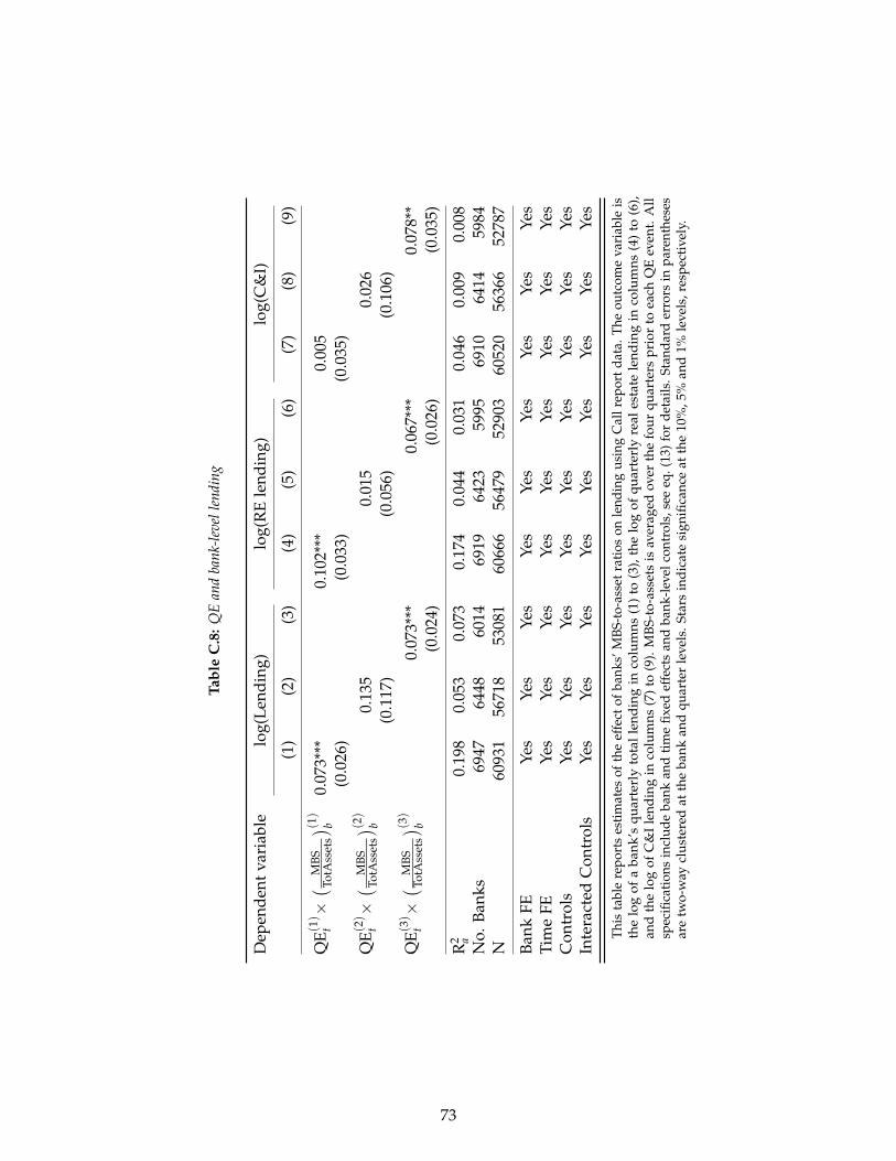
Tabl

eC

.8:Q

Ean

dba

nk-le

vell

endi

ng

Dep

ende

ntva

riab

lelo

g(Le

ndin

g)lo

g(R

Ele

ndin

g)lo

g(C

&I)

(1)

(2)

(3)

(4)

(5)

(6)

(7)

(8)

(9)

QE(1)

t×

( MBS

TotA

sset

s) (1) b0.

073*

**0.

102*

**0.

005

(0.0

26)

(0.0

33)

(0.0

35)

QE(2)

t×

( MBS

TotA

sset

s) (2) b0.

135

0.01

50.

026

(0.1

17)

(0.0

56)

(0.1

06)

QE(3)

t×

( MBS

TotA

sset

s) (3) b0.

073*

**0.

067*

**0.

078*

*(0

.024

)(0

.026

)(0

.035

)

R2 a

0.19

80.

053

0.07

30.

174

0.04

40.

031

0.04

60.

009

0.00

8N

o.Ba

nks

6947

6448

6014

6919

6423

5995

6910

6414

5984

N60

931

5671

853

081

6066

656

479

5290

360

520

5636

652

787

Bank

FEYe

sYe

sYe

sYe

sYe

sYe

sYe

sYe

sYe

sTi

me

FEYe

sYe

sYe

sYe

sYe

sYe

sYe

sYe

sYe

sC

ontr

ols

Yes

Yes

Yes

Yes

Yes

Yes

Yes

Yes

Yes

Inte

ract

edC

ontr

ols

Yes

Yes

Yes

Yes

Yes

Yes

Yes

Yes

Yes

This

tabl

ere

port

ses

timat

esof

the

effe

ctof

bank

s’M

BS-t

o-as

setr

atio

son

lend

ing

usin

gC

allr

epor

tdat

a.Th

eou

tcom

eva

riab

leis

the

log

ofa

bank

’squ

arte

rly

tota

llen

din

gin

colu

mns

(1)

to(3

),th

elo

gof

quar

terl

yre

ales

tate

lend

ing

inco

lum

ns(4

)to

(6),

and

the

log

ofC

&I

lend

ing

inco

lum

ns(7

)to

(9).

MB

S-to

-ass

ets

isav

erag

edov

erth

efo

urqu

arte

rspr

ior

toea

chQ

Eev

ent.

All

spec

ifica

tions

incl

ude

bank

and

time

fixed

effe

cts

and

bank

-lev

elco

ntro

ls,s

eeeq

.(13

)fo

rde

tails

.Sta

ndar

der

rors

inpa

rent

hese

sar

etw

o-w

aycl

uste

red

atth

eba

nkan

dqu

arte

rle

vels

.Sta

rsin

dica

tesi

gnifi

canc

eat

the

10%

,5%

and

1%le

vels

,res

pect

ivel

y.

73

Table C.9: QE and bank-level mortgage lending

Dependent variable log(Total) log(Refinance) log(Origination)

(1) (2) (3) (4) (5) (6)

QE(1)t ×

( MBSTotAssets

)(1)b 0.452*** 0.712*** 0.212

(0.161) (0.206) (0.148)

QE(3)t ×

( MBSTotAssets

)(3)b 0.229** 0.220* 0.214*

(0.113) (0.129) (0.127)

R2a 0.057 0.032 0.119 0.064 0.065 0.108

No. Banks 4178 3581 4039 3495 4102 3493N 24958 25449 22811 23206 23381 23780

Bank FE Yes Yes Yes Yes Yes YesTime FE Yes Yes Yes Yes Yes YesControls Yes Yes Yes Yes Yes YesInteracted Controls Yes Yes Yes Yes Yes Yes

This table reports estimates of the effect of banks’ MBS-to-asset ratios on mortgage lendingusing Home Mortgage Disclosure Act (HMDA) data. The outcome variable is the log of abank’s quarterly total mortgage lending in columns (1) and (2), the log of mortgage refinancingvolume in columns (3) and (4), and the log of mortgage origination volume in columns (5) to(6). MBS-to-assets is averaged over the four quarters prior to each QE event. All specificationsinclude bank and time fixed effects and bank-level controls, see eq. (13) for details. Standarderrors in parentheses are two-way clustered at the bank and quarter levels. Stars indicatesignificance at the 10%, 5% and 1% levels, respectively.

74

Table C.10: QE and bank-level small business lending

Dependent variable log(C&I lending)

Loan size [0, 100k] [100k, 250k] [250k, 1m] Rev<1mil

(1) (2) (3) (4) (5) (6) (7) (8)

QE(1)t ×

( MBSTotAssets

)(1)b -0.126 0.012 0.107 0.248*

(0.124) (0.120) (0.122) (0.150)

QE(3)t ×

( MBSTotAssets

)(3)b 0.137 0.183** 0.395*** 0.299**

(0.114) (0.089) (0.125) (0.134)

R2a 0.316 0.072 0.322 0.136 0.319 0.150 0.350 0.119

No. Banks 743 652 742 653 744 654 743 650N 1826 1674 1821 1674 1818 1681 1826 1665

Bank FE Yes Yes Yes Yes Yes Yes Yes YesTime FE Yes Yes Yes Yes Yes Yes Yes YesControls Yes Yes Yes Yes Yes Yes Yes YesInteracted Controls Yes Yes Yes Yes Yes Yes Yes Yes

This table reports estimates of the effect of banks’ MBS-to-asset ratios on mortgage lending using CommunityReinvestment Act (CRA) data. The outcome variable is the log of a bank’s total C&I loans with loan volumeless than $100k in columns (1) and (2), the log of total C&I loans with loan volume between $100k and $250k incolumns (3) and (4), the log of total C&I loans with loan volume between $250k and $1m in columns (5) and (6),and the log of total C&I loans to businesses with revenue less than $1m in columns (7) and (8). MBS-to-assets isaveraged over the four quarters prior to each QE event. All specifications include bank and time fixed effects andbank-level controls, see eq. (13) for details. Standard errors in parentheses are two-way clustered at the bank andquarter levels. Stars indicate significance at the 10%, 5% and 1% levels, respectively.

75

Table C.11: Firm-level regression: Investment and employment effects for firms in Y14 and for firmsmatched to Compustat

Panel A: Continous treatment


Sample Entire sample Not in SNC SNC sample

(1) (2) (3) (4) (5) (6)

QE(3) ×( MBS

TotAssets

)(3)b 0.344*** 0.402*** 0.301** 0.501*** 0.206*** 0.226***

(0.023) (0.054) (0.120) (0.145) (0.041) (0.046)




Sample Entire sample Not in SNC SNC sample

(1) (2) (3) (4) (5) (6)

QE(3)× Treat(3)b 0.022*** 0.026*** 0.021*** 0.030*** 0.024*** 0.022***(0.001) (0.004) (0.007) (0.011) (0.004) (0.004)


Bank-firm level analysis with firm-time fixed effect. Observation are restricted to 7 quarters, 3 quartersbefore and 3 quarters after QE3. Standard errors in parentheses are clustered at the firm-time leveland stars indicate significance at the 10%, 5%, and 1% level, respectively. We use the computationallyefficient estimator of linear models with multiple levels of fixed effects proposed by Correia (2017).

76

Appendix D Variable construction

Bank variables are from the merger-adjusted Consolidated Reports of Condition and Income (FFIEC031

and FFIEC041). Banks are indexed by b, time is indexed by t (quarters).

• Total securities (available for sale, fair value)b,t: RCFD1773

• Total securities (held to maturity, amortized cost)b,t: RCFD1754

• MBS (held to maturity, amortized cost)b,t: The sum of all item in Schedule RC-B, item 4, column A,

excluding items a.(3), b.(3), and c(1b) and c(2b).

• MBS (available for sale, fair value)b,t: The sum of all item in Schedule RC-B, item 4, column C,

excluding items a.(3), b.(3), and c(1b) and c(2b).

• Bank sizeb,t: the log of total assets: Log(RCFD2170)

• Return on Assetsb,t: Income (loss) before discontinued operations over assets: RIAD4300/RCFD2170

• Overhead ratiob,t: The ratio of Noninterest expense (RIAD4093) divided by revenue. Revenue is

the sum of net interest income (RIAD4074) and noninterest income (RIAD4079)).

• Net-interest marginb,t: The ratio of Annualized net interest income (RIAD4074) divided by (30-day

average) interest-earning assets (RCFD3381+ RCFDB558 + RCFDB559 + RCFDB560 + RCFD3365 +

RCFD3360 + RCFD3484 + RCFD3401)

• (Delinquencies/Loan Loss Reserves)b,t: The ratio of Delinquencies on all loans and leases (RC-N)

divided by reserves for loan losses (RCFD3123)

• Ratio of non-performing loansb,t: The sum of all loans that are past due 90 days or more and still

accruing (Schedule RC-N, Items 1 – 9 Column B) divided by total loans (RCFD2112)

• Equity ratiob,t: Total equity capital over assets: RCFDG105/RCFD2170

• Real estate loan ratiob,t: Loans secured by real estate over total loans and leases held for investment

and held for sale: RCFD1410/RCFD2122

• Deposit ratiob,t: Deposits in foreign and domestic offices over assets:

(RCON2200 + RCFN2200)/RCFD2170

77

• Loans Loansb,t: Total loans and leases held for investment and held for sale over assets:

RCFD2122/RCFD2170

• C&I Lendingb,t/Loansb,t: Commercial and industrial loans over total loans:

(RCFD1763+RCFD1764)/RCFD2122

• Tier 1 capital ratiob,t: RCFA7206

78

employment e ects of unconventional monetary … contrast, after qe1, no such differential effect is...

Documents