The Co-Movement and Causality between the U.S. Housing and

Stock Markets in the Time and Frequency Domains

Tsangyao Changa, Xiao-lin Lib, Stephen M. Millerc,

Mehmet Balcilard and Rangan Guptae

ABSTRACT

This study applies wavelet analysis to examine the relationship between the U.S. housing and stock markets over the period 1890-2012. Wavelet analysis allows the simultaneous examination of co-movement and causality between the two markets in both the time and frequency domains. Our findings provide robust evidence that co-movement and causality vary across frequencies and evolve over time. Examining market co-movement in the time domain, the two markets exhibit positive co-movement over recent decades, except for 1998-2002 when a high negative co-movement emerged. In the frequency domain, the two markets correlate with each other mainly at low frequencies (longer term), except in the second half of the 1900s as well as in 1998-2002, when the two markets correlate at high frequencies (shorter term). In addition, we find that the causal effects between the markets in the frequency domain occur generally at low frequencies (longer term). In the time-domain, the time-varying nature of long-run causalities implies structural changes in the two markets. These findings provide a more complete picture of the relationship between the U.S. real estate and stock markets over time and frequency, offering important implications for policymakers (and practitioners). Key words: stock market; housing market; wavelet analysis; frequency domain; time

domain JEL: C49, E44, G11 a Department of Finance, Feng Chia University, Taichung, Taiwan. Email: tychang@fcu.edu.tw. b Department of Finance, Ocean University of China, Qingdao, China. Email: smileman2004@126.com. c Corresponding author. Department of Economics, University of Nevada, Las Vegas, Las Vegas, Nevada, 89154-6005 USA, Email: stephen.miller@unlv.edu. d Department of Economics, Eastern Mediterranean University, Famagusta, Turkish Republic of Northern Cyprus, via Mersin 10, Turkey. Email: mehmet@mbalcilar.net. e Department of Economics, University of Pretoria, Pretoria, 0002, South Africa. Email: rangan.gupta@up.ac.za.

1

1. Introduction

This paper provides some fresh insights on the linkages between the U.S. housing and stock

markets. In the U.S. economy, housing and stock holdings comprise the two largest and

principal components of wealth. Movements in their market values can dramatically affect

the economic condition of families and businesses and, hence, affect the overall growth of the

U.S. economy. Booms and busts in housing and stock markets have always played an

important role in U.S. business cycle history. The most recent financial crisis and Great

Recession saw an economy-wide housing bubble bust followed by a remarkable stock market

crash, causing the U.S. and the world economies to suffer huge financial losses. Much of the

existing literature considers the relationships between the real estate (housing) and stock

markets from the perspective of investors who want to diversify their portfolios.1 Our focus

considers these linkages from the perspective of macroeconomic policy makers who want to

use movements in these markets to analyze the business cycle.2

Macroeconomic policymakers consider wealth as an important driver of the economy

and view asset prices as important predictors of the business cycle. Researchers have long

used the stock market in the US as a leading indicator of the business cycle. (Moore 1983;

Siegel 1991; Chauvet 1998-1999). Siegel (1991) determines that of the 41 recessions

observed since 1802, at least an 8-percent loss in stock returns preceded 38. On the negative

side, 12 false signals occurred using this criterion, where no recession followed. Seven of

these false signals happened after WWII. Other researchers consider the predictive ability of

house prices. For example, Leamer (2007) argues that “housing is the business cycle,”

1 Since stocks act as one of the most convenient investment vehicles with low transaction cost and high liquidity while housing acts as a ‘bulky’ asset with high transaction cost and low liquidity, the two assets typically appear in homebuyers’ and investors’ portfolios (Lin and Fuerst, 2012). The diversification benefits, however, hinge on the relationships between the two underlying markets. This paper identifies co-movements and causality in the time and frequency domains between these two markets in the U.S., using distinctive data and methods, and deriving new insights and implications for investment strategies and market forecasts. 2 Our annual data set from 1890 to 2012 provides information that more closely links to business cycle rather than portfolio diversification issues, although some information does emerge for the latter.

2

showing that significant declines in housing construction preceded 8 of the last 10

recessions.3 As another example, Iacoviello and Neri (2010) estimate a DSGE model and

consider the role of the housing market in the propagation of the business cycle. They

conclude that “… spillovers from the housing market to the broader economy are

non-negligible, concentrated on consumption rather than business investment, and have

become more important over time, …” (p. 57).

The recent research on the relationships between real estate and stock markets falls

into three main braches of inquiry. First, researchers employ linear and non-linear

cointegration techniques, such as Johansen, fractional, and threshold cointegration tests, to

determine whether the two markets integrate with or segment from each other (Ambrose et al.,

1992; Wilson and Okunev, 1999; Liow, 2006; Lin and Fuerst, 2012; Liow and Yang, 2005;

Tsai et al., 2012). Policymakers (and practitioners) will respond differently, depending on

whether these markets as integrated or segmented.4 Market integration means that a boom

(bust) in one market associates with a boom (bust) in the other market, combining to generate

bigger macroeconomic cycles, whereas market segmentation does not imply such linkages

between markets and, thus, to smaller, non-synchronized effects on the macroeconomy.

Second, researchers consider the linkages between real estate and stock markets by

applying Granger causality tests in vector autoregressive (VAR), vector error-correction

(VEC), and threshold error-correction (TEC) models (Gyourko and Keim, 1992; Okunev et

al., 2000; Sim and Chang, 2006; Su, 2011; Su et al., 2011; McMillan, 2012; Shirvani et al.,

2012; Tsai et al., 2012). The nature and direction of causality between the two markets can

aid policymakers and investors to forecast future performance from one market to the other

3 Even other views exist, however. Hamilton (2003, 2009) argues that oil price shocks proximately cause post-WWII recessions in the US. 4 Market integration means that a high degree of asset substitution exists between real estate and equities, while market segmentation implies the two assets provide good risk diversifiers for each other in portfolio management (Wilson et al., 1996).

3

through two transmission mechanisms (Chen, 2001; Case et al., 2005; Kapopoulos and Siokis,

2005). One, the “wealth effect” indicates that a rise in stock prices and, hence, an unexpected

gain in stock returns can boost real estate (housing) consumption and prices, while two, the

“credit-price effect” suggests that a rise in real estate (housing) prices can, in turn, lead to an

increase in stock market prices. Such feedback effects can aid booms and busts in these

markets, which feeds into macroeconomic cycles.

Third, researchers in earlier, less-sophisticated studies concentrate on the relationship

between real estate and stock markets through standard correlation analysis (Ibbotson and

Siegel, 1984; Hartzell, 1986; Eichholtz and Hartzell, 1996; Worzala and Vandell, 1993; Quan

and Titman, 1999).5 Although correlations can provide information about co-movement of

variables, it does not inform us about long-run relationships (i.e., cointegration) and/or the

lead-lag relationships (Granger causality) between the markets.

These existing studies exclusively utilize the conventional time-domain methods,

namely the above-mentioned cointegration techniques, causality tests, and correlation

analysis. Exceptions do occur, however. Liow (2012) adopts dynamic conditional correlation

(DCC) models to assess time-varying co-movement between the real estate and stock markets.

Louis and Sun (2013) examine simple correlations between housing and stock returns across

1-, 2-, 3-, and 4-year frequencies.6 That is, the existing literature typically ignores the

time-varying nature of the relationships between the two markets. Moreover, these

5 Correlation analysis interprets co-movement between the markets, which can suggest assets diversification benefits for investors. 6 Following the extant literature, we, too, consider a battery of standard time-series analyses. We run standard linear Granger causality tests in a VAR model of the real rates of return for house and stock prices, which Table A1 indicates are stationary, I(0), variables. Table A2 reports that the causality tests do not reject the null of no-causal relationship between the two variables. Further, we also test for cointegration between the natural logarithm of the real house and stock prices, which are nonstationary, I(1), variables. Table A3 shows that we cannot reject the null hypothesis of no-cointegration. Moreover, Table A4 reports evidence of instability of the long-run relationship estimated using fully-modified ordinary least squares method. Hence, the lack of causality does not reflect misspecification of the VAR in first-differences (growth rates) of the variables. Finally, Table A5 provides strong evidence of structural breaks in the individual equations of the VAR model, as well as the VAR model as a system, thus, invalidating the full-sample Granger causality result reported in Table A2. This, in turn, motivates the need for a time-varying approach to causality, which the wavelet analysis provides.

4

time-domain studies generally do not explore the frequency-variation in such relationships.

The time- and frequency-varying features in such relationships can provide important

implications for macroeconomic policymakers. The time-varying co-movement implies that

the variables contribute differently to the business cycle at different points in time. Thus,

policy makers need to consider both variables in their portfolio of business cycle predictors.

Frequency-varying co-movement suggests that when considering short- versus long-run

policy options, the policymakers need to monitor co-movement at different frequencies in the

markets and the macroeconomy.7

This paper utilizes a novel wavelet analysis to explore the relationship between the

U.S. housing and stock markets in both the time and frequency domains. Wavelet analysis

possesses significant advantages over conventional time-domain methods. It expands the

underlying time series into a time-frequency space where researches can visualize both time-

and frequency-varying information of the series in a highly intuitive way. Wavelet coherency

and phase differences simultaneously assess how the co-movement and causalities between

the U.S. housing and stock markets vary across frequencies and change over time in a

time-frequency window. In this way, we can observe high-frequency (short-term) and

low-frequency (long-term) relationships between the two markets as well as possible

structural changes and time-variations in such relationship.

Goffe (1994) and Ramsey and Lampart (1998a, b) introduce applications of wavelet

analysis in economics and finance. More recent work, however, focuses on the co-movement

between stock markets as well as between energy commodities and the macroeconomy (Rua

7 The time- and frequency-varying features in such relationships also can provide important practical implications for portfolio management. Time-varying co-movement implies that the risk exposure and diversification benefits of asset portfolios evolve over time and, thus, investors should incorporate such effects when evaluating the risk and returns of these portfolios. Frequency-varying co-movement suggests that investors with different investment horizons should consider the co-movement at corresponding frequencies so as to allocate their assets more effectively. The time- and frequency-varying features in the causality can also significantly affect the accuracy of market performance prediction and, hence, affect the investment benefits for practitioners and the regulatory benefits to policymakers.

5

and Nunes, 2009; Graham and Nikkinen, 2011; Aguiar-Conraria and Soares, 2011; McCarthy

and Orlov, 2012; Loh, 2013; etc.). To the best of our knowledge, one paper (Zhou 2010)

applies wavelet analysis to the relationship between real estate and stock markets. Zhou

(2010) assesses the co-movement between publicly traded real estate securities and stock

indexes for six countries and, thus, focuses on the portfolio diversification issues.

This study differs from the existing literature in several important ways. First, the

wavelet analysis devotes special and full attention to dynamic co-movement and causalities

between the U.S. housing and stock markets. Second, we use the distinctive annual data of

Robert Shiller’s housing and S&P stock returns over an extended from 1890 to 2012, which

implies that our findings apply for policymakers (and practitioners) in the residential real

estate and stock markets. Third, we employ the growth rate of GDP as a control variable to

remove the effects of economic growth on both the housing and stock markets performances

(Quan and Titman, 1999). Fourth, we also estimate the partial wavelet coherency and partial

phase difference as necessary complements to the common-used wavelet coherency and

phase difference. Finally, we perform a simultaneous assessment of the co-movement and

causal relationships between the two markets in the time and frequency domains.

This study contributes to the existing literature in several important ways. Our

empirical results show substantial time- and frequency-varying features in the co-movement

and causality between the U.S. housing and stock markets. This provides additional and

useful implications for policymakers.8 In addition, we identify the co-movement during the

recent financial crisis with the results showing that the two markets actually respond more to

economic growth fundamentals, rather than to each other.

This paper proceeds as follows. Section 2 briefly reviews the related literature.

Section 3 provides an overview of wavelet theory and methods. Section 4 describes the data 8 It also provides some insight for investment strategies and the forecasts of the markets' performance for investors.

6

and presents the empirical results. Section 5 concludes.

2. Literature Review

As mentioned above, a large literature exists to identify whether real estate and stock markets

are integrated or segmented through a variety of cointegration techniques. The results differ

widely depending on the datasets examined and the methodology used. Liu et al. (1990)

adopt the capital asset pricing model (CAPM) presented by Jorion and Schwartz (1986) and

find that segmentation does exist between the U.S. commercial real estate and stock markets

because of indirect barriers such as the cost, amount, and quality of information on real estate.

Geltner (1990) supports this segmentation hypothesis by documenting that the noise

component of the commercial real estate returns differ from the noise component of stock

returns. Ambrose et al. (1992) conclude on the contrary, however, that the securitized real

estate market may integrate with the stock market, using a rescaled range analysis to test

deterministic nonlinear trend in the underlying return series. Myer and Webb (1993) also

report a certain degree of integration between the two markets, noting that the returns on

equity Real Estate Investment Trusts (REITs) seem similar to the returns on common stocks.

Liow (2006) finds that the stock market integrates with the residential and office property

market in the Singapore economy, using the autoregressive distributed lag (ARDL)

cointegration procedure.

Okunev and Wilson (1997) develop a fractional cointegration test, which considers a

stochastic trend term instead of the deterministic drift term employed by Ambrose et al.

(1992). They conclude that the U.S. securitized real estate and stock markets fractionally

integrate with each other. Following their analysis, the literature widely employs the

non-linear fractional cointegration test. Wilson and Okunev (1999) apply this technique to

test for long-term relationship between the securitized real estate and stock markets for three

countries, finding segmented markets in the U.S. and the U.K., but somewhat integrated

7

markets in Australia. Lin and Fuerst (2012) apply both the fractional and Johansen’s (1988,

1991) cointegration tests, demonstrating that the stock market linearly integrates with the

property market in China, Japan and Thailand, but fractionally integrates in Singapore and

Hong Kong, and remains segmented in Taiwan, Malaysia, Indonesia and South Korea. In an

earlier study, Liow and Yang (2005) infer from the same fractional cointegration analysis that

the securitized real estate (indirect real estate) and stock markets in Singapore and Hong

Kong fractionally integrate with each other and, thus, the two underlying assets substitute

over the long term. Additionally, Tsai et al. (2012) use the momentum-threshold

autoregressive (M-TAR) method and find an asymmetric cointegration relationship between

the U.S. housing and stock markets.

A growing number of studies consider the causal link between the real estate and

stock markets. Gyourko and Keim (1992) suggest a causal link from the U.S. stock market to

real estate market by testing the S&P 500 and equity REITs return series. Okunev et al. (2000)

detect a strong unidirectional causality running from the U.S. stock market to the securitized

real estate market by employing nonlinear causality tests. Su (2011) conducts the non-linear

causality tests based upon the TEC model and provides evidence in favor of the credit-price

effect in Germany, the Netherlands, and the U.K., the wealth effect in Belgium and Italy, and

both effects in France, Spain, and Switzerland. Ibrahim (2010) confirms the wealth effect

channel for Thailand, using standard linear Granger causality tests. Tsai et al. (2012) also

perform the similar non-linear causality test in the context of TEC model, concluding that the

wealth effect dominates when the U.S. stock market outperforms the housing market.

McMillan (2012) adopts the exponential smooth transition (ESTR) procedure for non-linear

causality test, finding a unidirectional causality running from housing prices to stock prices in

the U.S. and the U.K., which implies a credit-price effect across the two economies. Shirvani

et al. (2012) report the presence of bilateral causality between the U.S. stock prices and

8

residential real estate prices. Kapopoulos and Siokis (2005) support the wealth effect

hypothesis for Athens housing prices but not for other Greek urban housing prices. Sim and

Chang (2006) provide evidence that most Korean regional housing and land markets Granger

cause stock prices in a VAR framework, which supports the credit-price hypothesis.

Bouchouicha (2013) constructs non-linear Markov switching models to assess the causal link

between the housing and stock markets in the U.S. and the U.K. with the maximum

likelihood (ML) estimations indicating that credit-price effect is stronger than wealth effect in

both countries. Along similar lines, Aye et al. (2013), based on nonparametric tests, find that

not only does the real house price cointegrate with the real stock price, but also bi-directional

causality exists between these two asset prices, even when standard linear cointegration and

Granger causality tests fail to pick up any relationship between these two asset prices.

In addition, from the time-domain, earlier studies investigate the correlation between

real estate and stock markets. Ibbotson and Siegel (1984), Hartzell (1986), and Eichholtz and

Hartzell (1996) show a negative correlation between the two markets for the U.S., the U.K.,

and Canada, whereas Worzala and Vandell (1993) find a positive correlation between the

U.K. real estate and stock markets. Quan and Titman (1999) support the positive correlation

between the two markets by estimating cross-sectional data from seventeen different

countries. More recently, Liow (2012) assesses the time-varying co-movement between the

securitized real estate and stock markets using the dynamic conditional correlation (DCC)

method, but neglects any frequency-varying features in markets co-movements.

Louis and Sun (2013) examine the relationship between the growth in state housing

prices and stock market returns of corporations with headquarters in that state, using quarterly

data from 1979 to 2002. They perform their analysis at different frequencies by considering

housing price growth and stock returns averaged over 1, 2, 3, and 4 years. They find that

housing price growth and stock returns exhibit a strong negative relationship that remains

9

robust to a series of alternative control variables, enabling investors to earn abnormal returns.

While the existing literature generally adopts time-domain analysis, Zhou (2010), the

closest study to our analysis in terms or methodology, uses wavelet analysis to evaluate the

co-movement between six publicly traded real estate securities – the U.S., the U.K., Japan,

Australia, Hong Kong, and Singapore as well as the co-movement between the securities and

the stock market indexes of the same country. The results indicate strong co-movement

across a large range of frequencies for Japan, Hong Kong, and Singapore, but only across a

limited band of frequencies for the U.S., the U.K. and Australia.

Although we use wavelet analysis, our paper differs from Zhou (2010) in several

important respects. First, we concentrate on the time- and frequency-varying features of both

the co-movement and causalities between the U.S. housing and stock markets; Zhou (2010)

examines the relationships between publicly traded real estate securities and stock markets.

Moreover, we employ the annual transaction-based Shiller housing returns and S&P stock

returns data from 1890 to 2012; Zhou (2010) uses monthly data from 1990 to 2009. Our

analysis provides insight as to macroeconomic business cycle analysis (and investor

decisions), whereas Zhou (2010) only considers investment decisions. Lastly, we use the

growth rate of GDP to control for the general economy's effect, attempting to extract the

direct real relationships between the two markets; Zhou (2010) does not use any control

variables.

3. Wavelet Theory and Methods

Wavelet analysis originated in the mid-1980s as an alternative to the well-known Fourier

analysis. Though Fourier analysis can uncover how relations vary across frequencies using

spectral techniques, the Fourier-transform analysis discards the time-localized information.

Moreover, Fourier analysis only applies to stationary series. In contrast, wavelet analysis

conducts the estimation of spectral characteristics of a time series as a function of time

10

(Aguiar-Conraria et al., 2008). It, therefore, can extract localized information in both time

and frequency domains. Moreover, wavelet analysis exhibits a significant advantage over

Fourier analysis, since it can accommodate non-stationary or locally stationary series (Roueff

and Sachs, 2011).

3.1 Continuous wavelet transform

The wavelet transform decomposes a time series into stretched and translated versions of a

given “mother wavelet” localized in time and frequency. In this way, the series is expanded

into a time-frequency space where its oscillations appear in a highly intuitive way. Two kinds

of wavelet transforms exist: discrete wavelet transforms (DWT) and continuous wavelet

transforms (CWT). The former reduces noise and compresses data whereas the latter extracts

features and detects data self-similarities (Grinsted et al., 2004; Loh, 2013).9 In this paper,

we choose the CWT to decompose the concerned series into wavelets. The CWT of a given

time series ( )tx is defined as:

( ) ( ) ( )∫+∞

∞−= dtttxsW sx

*,, tψt , (1)

where ( )ts*

,tψ is the complex conjugate function of ( )ts,tψ , ( )ts,tψ is the “daughter

wavelet” function derived from the mother wavelet function ( )tψ during the decomposition,

t is the location parameter that indicates where the mother wavelet is centered, and s is

the wavelet scale that defines how the “mother wavelet” is stretched. By varying the

parameter s and translating along the localized time index t , a picture shows both the

amplitude of any feature versus the scale and how this amplitude varies with time(Torrence 9 Feature extraction simplifies the resources required to describe a large set of data accurately. If we carefully choose the features to extract, then the features set will provide the relevant information from the input data to perform the desired task, using this reduced representation instead of the full-sized input. The self-similarity of a time series means the series exhibits long-term dependence (i.e., the whole series possesses the same shape, such as wave and cycle, as one or more of its parts). Taking advantage of feature extraction and self-similarity detection, the CWT extracts the local amplitudes of a time series (e.g., business cycle series) in time and frequency domains. Then, the ensuing wavelet coherency and phase difference tools measure whether and how the local amplitudes of two time series correlate, and which one leads.

11

and Compo, 1998). Moreover, since s and t are continuous values, ( )sWx ,t is called

accordingly as CWT. The relationship between ( )ts,tψ and ( )tψ is written as:

( )

−

=s

ts

t tψψt1

s，, (2)

As the mother wavelet of the CWT, ( )tψ must satisfy the admissibility condition as follows:

( )+∞= ∫

∞+

ωωωψ

ϕ dC0

2

0 , (3)

where ( )ωψ is the Fourier transform of the mother wavelet ( )tψ .

Various types of mother wavelets exist for various purposes, such as the Haar, Morlet,

Daubechies, Mexican hat, and so on wavelets. Among them, the most popular and applicable

mother wavelet for feature extraction is the Morlet wavelet, which Grossman and Morlet

(1984) introduce and define as follows:

( ) 2-41- 20 tti eet ωπψ = , (4)

where 2- 2te ensures that it satisfies the admissibility condition of equation (3) (Farge, 1992).

In particular, when the dimensionless frequency 0ω equals 6, the Morlet wavelet achieves

optimal trade-off between time and frequency localization (Grinsted et al., 2004).

According to Aguiar-Conraria and Soares (2013), the Fourier frequency

( ) ssf πω 20= . Therefore, the best conversion from the wavelet scale s to the Fourier

frequency f occurs when 60 =ω in the sense that:

ssf 126 ≈= π , (5)

As a result, the wavelet scale approximates a reciprocal of the Fourier frequency. That is,

12

( )tx decomposes into a joint time-frequency plane, where the shorter (longer) wavelet scale

corresponds to the higher (lower) frequency. Moreover, since the Morlet wavelet is a complex

wavelet, the CWT divides into real and imaginary parts. As such, we can calculate the

amplitudes and phases of the CWT for further estimations of wavelet power spectrum,

wavelet coherency, and phase difference.

3.2 Wavelet power spectrum

The wavelet power spectrum of one series ( )tx , namely the auto-wavelet power spectrum,

equals ( ) 2, sWx t . It presents a measure of the localized variance (volatility) of ( )tx at each

scale or frequency. Furthermore, since Hudgins et al. (1993) first introduce the cross-wavelet

transform of ( )tx and ( )ty as ( ) ( ) ( )sWsWsW yxxy ,,, * ttt = , we can write the cross-wavelet

power spectrum as follows:

( ) ( ) ( )2*22

,,, sWsWsW yxxy ttt = , (6)

where the asterisk indicates the complex conjugation. The cross-wavelet power spectrum can

give a measure of the localized covariance between ( )tx and ( )ty for the specified

frequency.

In this paper, the wavelet power spectrum depicts the localized volatility of the U.S.

real housing and stock returns as well as estimates the wavelet coherency between the two

returns. Note that, in wavelet power spectrum plots, we mark the wavelet power of the real

housing and stock return series by colors, where red and blue colors correspond to high and

low power. Therefore, the colors correspond to the localized volatility of the underlying

series.

3.3 Wavelet coherency and phase difference

Wavelet coherency allows for a three-dimensional analysis, which simultaneously considers

13

the time and frequency components, as well as the strength of correlation between the

time-series components (Loh, 2013). In this way, we can observe both the time- and

frequency-variations of the correlation between series in a time-frequency space.

Consequently, the wavelet coherency provides a much better measure of co-movement

between the U.S. real housing and stock returns in comparison to the conventional correlation

analysis as well as the dynamic conditional correlation analysis (Zhou, 2010; Liow, 2012;

Loh, 2013). Following the approach of Torrence and Webster (1999), we estimate wavelet

coherency by using the cross-wavelet and auto-wavelet power spectrums as follows:

( )( )( )

( )( ) ( )

=−−

−

2121

21

2

,,

,,

xWsSsWsS

sWsSsR

yx

xy

xy

tt

tt . (7)

We calculate wavelet coherency with the above squared expression with smoothing

operator S .10 In this way, it generates a value between 0 and 1 in a time-frequency window.

Zero coherency indicates no co-movement between the real housing and stock returns, while

the highest coherency implies the strongest co-movement between the two returns. In the

empirical section, we also clearly mark the squared wavelet coherency with colors in the

wavelet coherency plots, where red and blue colors correspond to strong and weak

co-movements, respectively.

The wavelet coherency cannot distinguish between positive and negative

co-movements, since it squares all terms. Therefore, we subsequently use the phase

difference to provide information on positive and negative co-movements as well as the

lead-lag relationships between the two returns. According to Bloomfield et al. (2004), the

phase difference characterizes phase relationship between ( )tx and ( )ty such that:

10 Without smoothing, the squared wavelet coherence always equals 1 at any frequency and time. We convolute in time and frequency to achieve smoothing; see Torrence and Compo (1998) for details.

14

( )( )}{( )( )}{

ℜ

ℑ= −

−−

sWsSsWsS

xy

xyxy ,

,tan 1

11

tt

φ , with [ ]ππφ ，-∈xy , (8)

where ℑ and ℜ equal the imaginary and real parts of the smoothed cross-wavelet

transform, respectively.

A phase difference of zero indicates that the two underlying series move together

while a phase difference of π ( π− ) implies that they move in the opposite directions. If

( )2,0 πφ ∈xy , then the series move in phase (positively co-move) with ( )tx leading ( )ty .

If ( )ππφ ,2∈xy , then the series move out of phase (negatively co-move) with ( )ty leading

( )tx . If ( )2, ππφ −−∈xy , then the series move out of phase with ( )tx leading ( )ty . If

( )0,2πφ −∈xy , then the series move in phase with ( )ty leading ( )tx . Note that the phase

difference can also indicate causality between ( )tx and ( )ty in both the time and frequency

domains. As a consequence, it dominates the conventional Granger causality test, which

assumes that a single causal link holds for the whole sample period as well as at each

frequency (Grinsted et al., 2004; Tiwari et al., 2013). For example, in wavelet analysis, if

( )tx leads ( )ty , then a causal relationship runs from ( )tx to ( )ty at a particular time and

frequency.

Given that economic fundamentals could significantly affect both the U.S. real

housing and stock returns, we, therefore, want to eliminate the effects of economic growth to

uncover the real co-movement and causality between the two returns. For this purpose, we

rely on partial wavelet coherency and partial phase difference extensions of wavelet

coherency and phase difference, respectively. According to Aguiar-Conraria and Soares

(2013), we can define the squared partial wavelet coherency between ( )tx and ( )ty after

controlling the series ( )tz as follows:

15

( )( ) ( ) ( )

( )( )( ) ( )( )( )22

2*2

,1,1

,,,,

sRsR

sRsRsRsR

yzxy

yzxzxyzxy tt

tttt

−−

−= , (9)

where ( )sRxz ,t and ( )sRyz ,t indicate the wavelet coherencies between ( )tx and ( )tz and

between ( )ty and ( )tz , respectively. Accordingly, we can also represent the partial phase

difference as follows:

( )( )( )( )

ℜ

ℑ= −

sC

sC

zxy

zxyzxy ,

,tan 1

t

tφ , (10)

where ℑ and ℜ equal the imaginary and real parts of the complex partial wavelet

coherency ( )sC zxy ,t , respectively. The complex partial wavelet coherency, as the name

implies, is the complex type of ( )sR zxy ,t before taking the absolute value.

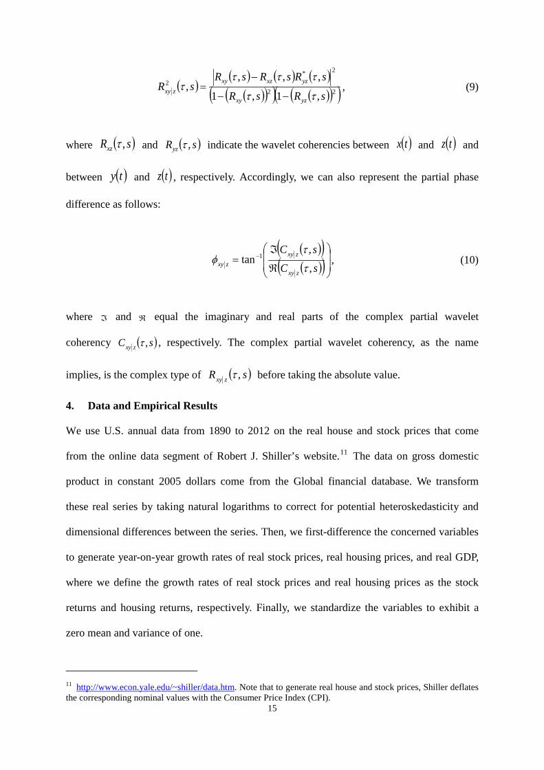
4. Data and Empirical Results

We use U.S. annual data from 1890 to 2012 on the real house and stock prices that come

from the online data segment of Robert J. Shiller’s website.11 The data on gross domestic

product in constant 2005 dollars come from the Global financial database. We transform

these real series by taking natural logarithms to correct for potential heteroskedasticity and

dimensional differences between the series. Then, we first-difference the concerned variables

to generate year-on-year growth rates of real stock prices, real housing prices, and real GDP,

where we define the growth rates of real stock prices and real housing prices as the stock

returns and housing returns, respectively. Finally, we standardize the variables to exhibit a

zero mean and variance of one.

11 http://www.econ.yale.edu/~shiller/data.htm. Note that to generate real house and stock prices, Shiller deflates the corresponding nominal values with the Consumer Price Index (CPI).

16

Figures 1, 2, and 3 report the time-series plots and auto-wavelet power spectrums of

real stock returns, real housing returns, and real economic growth, respectively. The thick

black lines in the wavelet power spectrum plots designate the 5-percent significance level

estimated from Monte Carlo simulations using a phase randomized surrogate series. The

regions below the thin black lines are cones of influence (COI) in which edge effects exist.12

As mentioned before, we employ the wavelet power spectrum as an indicator of the local

volatility of underlying series.

Figure 1 shows that U.S. stock returns exhibit high wavelet power across the 3-10 year

frequency band during the interwar period. Within this period, the great bull market, which

most analysts regard as the biggest stock-market bubbles of all time, crashed in 1929 and the

stock prices fluctuated dramatically until 1939. In the 1970s, the power of stock returns

increase, as a result of the severe oil price shocks in 1973 and 1978. During the 2000s, the

high wavelet power across the 6-8 year frequency band corresponds to the recent remarkable

boom-bust cycle in the stock market.

Figure 2 indicates that a relatively high wavelet power of U.S. housing returns exists

before the 1950s. Before World War I, we see high power across the 2-6 year frequency band,

as a result of a succession of boom-bust fluctuations in the U.S. housing market during this

period. At the end of World War II, the housing returns exhibit rapid growth in the mid-1940s,

subsequently collapsing in 1947. After that, the volatility of housing returns declines

significantly except over the 1970s and 1980s, when the housing returns rise above and fall

below zero in the late 1970s and late 1980s. Most recently, the great housing bubble peaks

around the beginning of 2006 and finally busts at the end of 2006, creating the worst housing

12 Following Torrence and Compo (1998) and Grinsted et al. (2004), the CWT assumes that the time series are cyclical. When transforming and plotting wavelets for the series with finite length, the amplitudes inside the COI drop by a factor 2e− due to zero padding at the edge. In addition, the edge effects are inversely proportional to the frequency. Therefore, we must pay special attention not to misread results inside the COI, especially at lower frequencies.

17

crash in U.S. history.

Figure 3 shows that U.S. economic growth exhibits high power across the 2-8 year

frequency band until the 1950s. The extremely high power at lower frequencies between the

1930s and the 1950s corresponds with the “Great Depression,” marking the deepest and

longest-lasting economic downturn in history. After that, the volatility of economic growth

declines steadily. Since the 1980s, the volatility decreased significantly at all frequencies,

corresponding to the “Great Moderation” (Blanchard and Simon, 2001). As Aguiar-Conraria

et al. (2008) find, we also observe that the Great Moderation associates with a secular rather

than decadal trend.

In general, the wavelet power spectrums yield consistent results with the time plots,

reflecting several major booms and busts in the U.S. housing and stock markets within the

sample period. Meanwhile, the stock returns also appear to associate with housing returns for

several sub-periods. We cannot determine, however, the co-movement and lead-lag

relationships, which can indicate causality, between the two markets through the wavelet

power spectrums. Therefore, we resort to wavelet coherency and phase difference between

the U.S. real housing and stock returns, where the results of estimation appear in Figure 4.13

Remember that the correlated regions inside the COI and above 10-percent significance level

do not provide reliable indications of co-movement and causality.

Figure 4 shows positive and strong co-movement between the U.S. housing and stock

returns. The co-movement, however, does depend on the frequency and is unstable over the

period 1890 to 2012. More specifically, from 1903-1910 and 1915-1933, the two returns

show an average coherency of 0.8 across the 3-6 year frequency band with an in-phase

relation indicated by the phase difference between 2π− and 2π , implying a high degree

of co-movement despite frequent boom-bust fluctuations in the two markets during these two 13 We thank Professors Aguiar-Conraria and Soares for providing the wavelet package to plot the wavelet coherency and phase difference between U.S. stock and housing returns.

18

periods. From 1938-1955, we observe positive co-movement scattered across the 2-10 year

frequency band with an average coherency of 0.7. After that, such co-movements appear

temporarily around the 3 year frequency band from 1973-1978, when the severe oil prices

shock greatly contributed to the U.S. housing market instabilities and the two successive

stock-market decreases in 1973 and 1974, as well as from 1984-1991, when the U.S. stock

market crashed in 1987 and almost at the same time the housing returns also went through a

temporary drop until 1992. Then, in the last decade, we find an increased coherency of 0.9

and an in-phase relationship both at high and low frequencies, meaning that the two returns

positively and highly co-move during the financial crisis. These findings support the

existence of time- and frequency-varying features in the correlations between U.S. real

housing and stock returns, but prove largely inconsistent with the findings of Ibbotson and

Siegel (1984), Hartzell (1986), and Eichholtz and Hartzell (1996), who suggest a single

positive or negative co-movement between the U.S. markets for the specified sample periods.

Figure 4 also shows an interesting picture of causality between U.S. real housing and

stock returns. In the 1900s, the stock returns lead the housing returns across the 4-6 year

frequency band, suggesting that returns in the stock market significantly affect the returns in

the housing market during this period. On the contrary, from 1915-1933, housing returns lead

stock returns at the 3-6 year frequency band, indicating that returns in the housing market

affect returns in the stock market. After that, at high frequencies, we see the causal link

running from stock to housing returns repeatedly for several periods -- 1938-1955, 1973-1976,

1984-1991, and 2000-2004. In the most recent decade, however, we find the reverse causal

link from housing to stock returns both at the 2-4 year and 6-7 year frequency bands. This

provides evidence that U.S. real housing returns significantly affect real stock returns over

the last ten years, especially for 2007-2010. The great housing-bubble bust leads to the

remarkable stock market crash. Overall, as displayed in Figure 4, substantial time- and

19

frequency-variations do exist in the causal relationship between real housing and stock

returns, which largely contradicts the findings of Shirvani et al. (2012) and Bouchouicha

(2013), who suggest a stable causality between the U.S. residential real estate and stock

markets holds in the whole sample period.

The fundamentals of economic growth, however, can significantly influence the U.S.

housing and stock markets and, hence, the relationship between the two markets' returns

(Quan and Titman, 1999). This implies that the above results estimated by wavelet coherency

and phase difference without removing the simultaneous effects of economic growth on the

two returns may suffer from inaccuracy. As a result, we further estimate the partial wavelet

coherency and partial phase difference with real GDP growth as a control variable to reveal

the relationship between the two returns. Figure 5 reports the findings.14 Once again, we note

that the correlated regions inside the COI and above 10-percent significance level do not

provide reliable information on co-movement and causality.

After controlling for real economic growth, Figure 5 shows that the co-movement

between U.S. real housing and stock returns differs substantially from the previous results.

From 1905 to 1910, we find that the high degree of positive co-movement increases at the 1-2

year frequency band, but decreases at low frequencies, compared to our prior findings. This

reveals that within this period U.S. real housing and stock returns keep strong co-movement

over the short term. From 1915-1933, the positive co-movement found previously decreases

significantly after removing the effects of economic growth, with a negatively correlated

region only from 1918 to 1922. We do see an increased and stable co-movement from 1933

to 1948, in contrast with the scattered co-movement over the same period without controlling

for economic growth. Moreover, unlike the previous result indicating insignificant and low

co-movement at low frequency from the late 1950s to the late 1970s, we now clearly see a

14 We estimate the partial wavelet coherency and partial phase difference between U.S. real stock and housing returns using the wavelet package kindly provided by Professors Aguiar-Conraria and Soares.

20

high degree of long-term co-movement indicated by the partial wavelet coherency. More

interestingly, we see the unusually negative co-movement indicated by the partial phase

difference from 1998 to 2002, when the housing market experienced steady growth whereas

the stock market slumped and finally crashed in 2000. Moreover, we do not observe any

significant co-movement across all frequencies during the most recent financial crisis. This

may imply that U.S. real housing and stock returns actually respond more to economic

growth fundamentals, rather than respond significantly to each other during these years. In

other words, the great housing bubble and its bust, as well as the stock market boom and

crash in the recent decade may depend fundamentally on the business cycle movements of

real GDP.

The causality between the U.S. real housing and stock returns shows distinctive

properties after controlling for economic growth. From 1905 to 1910, we see a short-run

causality running from stock returns to housing returns, indicating that the stock market leads

the housing market in the short run. From 1918 to 1922, the housing returns leads stock

returns at the 3-4 year frequency band. however, That lead-lag relationship inverts at lower

frequencies, however. From 1932 to 1948, the causality running from housing returns to

stock returns becomes relatively stable over the long term, instead of an unstable and even

inverse causal relationship before controlling for economic growth. Between the late 1950s

and the late 1970s, a significant time-variation exists in the causal relationship between the

two returns. Before the early 1960s, housing returns lead stock returns; in the later 1960s and

1970s, it lags behind stock returns. During the Great Moderation, we find that real housing

returns lead real stock returns rather than the reverse, which we find when we do not control

or economic growth. From 1998 to 2002, the housing returns significantly lead stock returns,

resulting in a shift in money from the stock market into the housing market.

In sum, whether we control for economic growth or not, the above results provide

21

robust evidence that the co-movement between U.S. real housing and stock returns indeed

varies across frequencies and evolves over time. In the time domain, the two returns generally

show positive co-movement except from 1998 to 2002, when a high degree of negative

co-movement exists. Understanding markets co-movement and further distinguishing

between positive and negative co-movement provides important practical information for

policy makers. Positive (negative) co-movements imply that booms and busts in the two

markets will reinforce (offset) each other in their effects on the business cycle.15

In the frequency domain, the two markets correlate with each other mainly at lower

frequencies (the 2-10 year frequency band) except from 1905 to 1910 and 1998 to 2002,

when the two markets correlate at high frequencies (i.e., short term).

The above analysis provides further robust evidence of causalities between U.S. real

housing and stock returns by using (partial) phase differences. The causality between the two

returns helps policymakers (and investors) to forecast future performance from one market to

the other through two transmission mechanisms, the “wealth effect” and “credit-price effect”.

The wealth effect means a transmission channel running from the stock market to the housing

market. Housing serves as an investment and consumption good, while stocks do not involve

direct consumption (Benjamin et al., 2004). As such, a rise in stock prices and, hence, an

unexpected gain in stock returns increases housing consumption and prices. The credit-price

effect implies that a rise in housing prices leads to an increase in stock market prices. That is,

when housing serves as collateral, an increase in its value will reduce the cost of borrowing

and enable credit-constrained households to increase consumption, leading to a rise in stock

15 Portfolio managers benefit as well. Since stocks provide the most convenient investment vehicle with low transaction costs and high liquidity while housing provides a ‘bulky’ asset with high transaction costs and low liquidity, homebuyers and investors use the two assets to diversify their portfolios (Lin and Fuerst, 2012). The diversification gain, however, depends on the nature and degree of the two markets co-movement. More specifically, it declines as the co-movement between the two assets become increasingly positive, but becomes important in the presence of low or negative co-movement. As a consequence, we can infer from our findings that a relatively low diversification gain emerges from the diversification of stocks and housing assets in the U.S. over our sample with the exception from 1998 to 2002 when the U.S. stock market dipped and investors accordingly became more active in the housing market.

22

prices.16

In this paper, we do not find any stable causality holding for the whole sample period.

Rather, the causality findings exhibit substantial time- and frequency-dependence. From the

frequency domain, causal effects exist between U.S. real housing and stock returns generally

across lower frequencies (i.e. long term). Thus, market performance forecasts should focus on

longer time horizons so as to enhance the forecasting accuracy of policymakers (and

investors). From the time domain, the time-varying nature in the long-run causalities between

U.S. real housing and stock returns implies structural changes in the two markets. We

observe the structural changes, referring to a long-term shift in the relationship between the

two returns, intuitively from the partial phase difference at the 4-8 year frequency band in

Figure 5(b). Before the mid-1920s, we find for several sub-periods causality running from

stock returns to housing returns, indicating the presence of wealth effect. After that, a

structural change occurs. The credit-price effect dominates in the U.S. economy until the

early 1960s, especially from 1932 to 1948 and from the late 1960s when statistically

significant effects exist. The wealth effect reappears, however, between the 1960s and the

1970s. Thereafter, we cannot identify any significant structural changes in the causality

between the two markets.

5. Conclusion

This paper provides fresh new insights into the relationship between the U.S. housing and

stock markets from 1890 to 2012, applying the novel wavelet analysis. That is, since the

16 The identification of the co-movement between the markets at different frequencies is clearly pivotal for investors, since it suggests that investors with different investment horizons should pay more attention to the co-movement at corresponding frequencies so as to allocate their assets more effectively. More specifically, if investors prefer the short-term investment horizon, then they should focus on the co-movement at higher frequencies and, hence, the economic factors driving such co-movement. On the other hand, if investors prefer the long-term investment horizon, then they should focus on the co-movement at lower frequencies and the corresponding driving factors (Smith, 2001). As a result, our findings regarding the co-movement between the U.S. housing and stock markets mainly across lower frequency bands imply that using stocks and real estate to diversify portfolios in the U.S. should focus on a long-term time horizon. In other words, the diversification gains from investing in stocks and housing will prove more attractive to long-term investors, such as pension funds, insurance companies, and other institutions, rather than short-term investors.

23

presence of structural breaks made the result of non-causality between these two asset returns

from standard linear Granger causality tests invalid, we need to adopt a time-varying

approach. Wavelet analysis allows a simultaneous assessment of co-movement and causality

between the two returns in both the time and frequency domains. Given that both U.S. real

housing and stock returns could respond significantly to changes in the fundamentals of

economic growth, we also control for the growth rate of GDP to reveal the true relationships

between the two returns by means of the partial wavelet coherency and partial phase

differences.

We do find that the co-movement between the two returns varies across frequencies

and evolves with time. From the time domain, the two returns exhibit positive co-movement

over 1890 to 2012 with an exception from 1998 to 2002 when negative co-movement occurs.

From the frequency domain, the two markets correlate with each other mainly at lower

frequencies with the exceptions from 1905 to 1910 and 1998 to 2002, when the two markets

exhibit correlation over the short term. 17 More specifically, we also find that the

co-movement during the recent financial crisis decreases significantly after controlling for

economic growth, suggesting that the two markets actually respond more to economic growth

fundamentals rather than respond significantly to each other during these years.

Louis and Sun (2013) uncover a negative relationship between the growth in housing

prices and stock returns in their state-level analysis at what they call the longer terms (4

years). Four years falls in the lower middle frequency of our 8-year frequency span. Thus,

while we consider national data on stock returns and housing price growth, we find this

negative correlation during the 1998 to 2002 period, which falls at the end of the sample of

Louis and Sun (2013). Our analysis suggests that this negative correlation appears as an

17 The time-domain findings suggest, in general, that lower diversification gains emerge from combining stocks and housing assets in a portfolio. But, the frequency-domain findings suggest that combining stock and housing in a portfolio achieves more diversification generally at the long-term horizon.

24

anomalous finding over our much longer sample.

We do not find any stable causal links between U.S. real housing and stock returns for

the whole sample. Rather, substantial time- and frequency-dependence effects exist. In other

words, policy makers cannot rely on the stock or housing market movements as the

proximate drivers of the business cycle, since we do not find any stable causal linkages.18 In

the frequency domain, the causal effects occur between the two returns generally across

lower frequencies (i.e., long term), implying that market performance forecast should focus

on a longer time horizon so as to enhance the forecasting accuracy of policymakers (and

investors). From the time domain, the time-varying features in the long-run causalities

between the two returns imply structural changes in the two markets.

References

Ambrose, B., Ancel, E., Griffiths, M. (1992). The fractal structure of real estate investment trust returns: a search for evidence of market segmentation and nonlinear dependency. Journal of the American Real Estate and Urban Economics Association, 20(1), 25-54.

Aguiar-Conraria, L., Azevedo, N., Soares, M. J. (2008). Using wavelets to decompose the

time-frequency effects of monetary policy. Physica A: Statistical Mechanics and its Applications, 387, 2863-2878.

Aguiar-Conraria, L., Soares, M. J. (2011). Oil and the macroeconomy: using wavelets to

analyze old issues. Empirical Economics, 40, 645-655. Aguiar-Conraria, L., Soares, M. J. (2013). The continuous wavelet transform: moving beyond

uni- and bivariate analysis, Journal of Economic Surveys, 00 (0), 1-32. Andrews, D. W. K. (1993). Tests for parameter instability and structural change with

unknown change point. Econometrica, 61, 821–856. Andrews, D. W. K. and Ploberger, W. (1994). Optimal tests when a nuisance parameter is

present only under the alternative. Econometrica, 62, 1383–1414.

18 As noted above, Hamilton (2003, 2009) argues that oil prices, which we do not consider in this paper, proves the proximate cause of the business cycle.

25

Aye, G. C., Balcilar, M., Gupta, R. (forthcoming). Long- and Short-Run Relationships between House and Stock Prices in South Africa: A Nonparametric Approach. Journal of Housing Research.

Benjamin, J., Chinloy, P., Jud, D. (2004). Why do households concentrate their wealth in

housing? Journal of Real Estate Research, 26, 329-344. Blanchard, O., Simon, J. (2001). The long and large decline in U.S. output volatility,

Brookings Papers on Economic Activity, 1,135-164. Bloomfield, D., McAteer, R., Lites, B., Judge, P., Mathioudakis, M., Keena, F. (2004).

Wavelet phase coherence analysis: application to a quiet-sun magnetic element. The Astrophysical Journal, 617, 623-632.

Bouchouicha, R. (2013). Dynamics of real estate markets and stock markets in the US and the

UK. Working paper series. Case, K. E., Quigley, J. M., Shiller, R. J. (2005). Comparing wealth effects: the stock market

versus the housing market. Advances in Macroeconomics, 5(1), 1-32. Chauvet. M., (1998-1999). Stock market fluctuations and the business cycle. Journal of

Economic and Social Measurement, 25, 235-257. Chen, N. (2001). Asset price fluctuations in Taiwan: evidence from stock and real estate

prices 1973 to 1992. Journal of Asian Economics, 12, 215-232. Eichholtz, P. M., Hartzell, D. J. (1996). Property shares, appraisals and the stock market: an

international perspective. The Journal of Real Estate Finance and Economics, 12(2), 163-178.

Farge, M., 1992: Wavelet transforms and their applications to turbulence. Annu. Rev. Fluid

Mech., 24, 395-457. Geltner, D. (1990). Return risk and cash flow with long term riskless leases in commercial

real estate. Journal of the American Real Estate and Urban Economics Association, 18(4), 377-402.

Grossman, A., Morlet, J. (1984). Decomposition of Hardy functions into square integral

wavelets of constant shape. SIAM J. Math. Anal., 15 (4), 723-736. Goffe, W. (1994). Wavelets in macroeconomics: an introduction. In D. Belsley (Ed.),

Computational Techniques for Econometrics and Economic Analysis, Kluwer Academic, 137-149.

Graham, M., Nikkinen, J. (2011). Co-movement of Finnish and international stock markets: a

wavelet analysis. European Journal of Finance, 17, 409-25. Grinsted, A., Moore, J. C., Jevrejeva S. (2004). Application of the cross wavelet transform

and wavelet coherence to geophysical time series. Nonlinear Process Geophysics, 11, 561-566.

26

Gyourko, J., Keim, D. (1992). What does the stock market tell us about real estate returns?

Journal of the American Real Estate Finance and Urban Economics Association, 20(3), 457-486.

Hamilton, J. D., (2003). What Is an Oil Shock? Journal of Econometrics 113, 363–398. Hamilton, J. D., (2009). Causes and Consequences of the Oil Shock of 2007–08. Brookings

Papers on Economic Activity (Spring), 215-261. Hansen, B. E. (1992) Tests for parameter instability in regressions with I(1) processes.

Journal of Business and Economic Statistics, 10, 321-336. Hartzell, D. (1986). Real estate in the portfolio, in F. J. Fabozzi, eds., The Institutional

Investor: Focus on Investment Management, Ballinger, Cambridge, Massachusetts. Hudgins, L., Friehe C., Mayer, M. (1993). Wavelet transforms and atmospheric turbulence.

Physical Review Letters, 71 (20), 3279-3282. Iacoviello M., Neri, S., (2010). Housing market spillovers: Evidence from an estimated

DSGE model. American Economic Journal: Macroeconomics 2(2): 125-164. Ibbotson, R. G., Siegel, L. B. (1984). Real estate returns: a comparison with other

investments. Real Estate Economics, 12(3), 219-242. Ibrahim, M. H. (2010) House price-stock price relations in Thailand: An empirical analysis.

International Journal of Housing Markets and Analysis, 3 (1), 69-82. Johansen, S. (1988). Statistical analysis of co-integration vectors, Journal of Economic

Dynamics and Control, 12, 231-54. Johansen, S. (1991). Estimation and hypothesis testing of cointegration vectors in Gaussian

vector autoregressive models. Econometrica, 59, 1551-1580. Jorion, P., Schwartz, E. (1986). Integration vs. segmentation in the Canadian stock market”.

Journal of Finance, 41(3), 603-616. Kapopoulos, P., Siokis, F. (2005). Stock and real estate prices in Greece: wealth versus

credit-price effect. Applied Economics Letters, 12(2), 125-128. Leamer, E. E., (2007). Housing is the business cycle. In Housing, Housing Finance, and

Monetary Policy, Economic Symposium Conference Proceedings, Kansas City Federal Reserve Bank, 149-233.

Lin, P. T., Fuerst, F. (2012). The integration of direct real estate and stock markets in Asia.

Working paper series. Liow, K. H., Yang, H. S. (2005). Long-term co-memories and short-run adjustment:

securitized real estate and stock markets. The Journal of Real Estate Finance and Economics, 31(3), 283-300.

27

Liow, K. H. (2006). Dynamic relationship between stock and property markets. Applied

Financial Economics, 16(5), 371-376. Liow, H. K. (2012). Co-movements and correlations across Asian securitized real estate and

stock markets. Real Estate Economics, 40(1), 97-129. Liu, C. H., Hartzell, D. J., Greig, W., Grissom, T. V. (1990). The integration of the real estate

market and the stock market: some preliminary evidence”, Journal of Real Estate Finance and Economics, 3(3), 261-282.

Loh, L. (2013). Co-movement of Asia-Pacific with European and US stock market returns: a

cross-time-frequency analysis. Research in International Business and Finance, 29, 1-13. Louis, H., Sun, A. X., (2013). Long-Term Growth in Housing Prices and Stock Returns. Real

Estate Economics, 41, 663–708. MacKinnon, J. G., Haug, A. A., Michelis, L. (1999) Numerical distribution functions of

likelihood ratio tests for cointegration. Journal of Applied Econometrics, 14, 563-577. McCarthy, J., Orlov, A. G. (2012). Time-frequency analysis of crude oil and S&P500 futures

contracts. Quantitative Finance, 12(12), 1893-1908. McMillan, D. (2012). Long-run stock price-house price relation: evidence from an ESTR

model. Economics Bulletin, 32(2), 1737-1746. Moore, G. H., (1983). Security markets and business cycles. In Business Cycles, Inflation,

and Forecasting, 2nd edition. (Ed.) Moore, G. H., NBER Book Series Studies in Business Cycles, 139-160.

Myer, F. C. N., Webb, J. R. (1993). Return properties of equity REITs, common stocks, and

commercial real estate: a comparison. Journal of Real Estate Research, 8(1), 87-106. Ng, S., Perron, P., 2001. Lag length selection and the construction of unit root tests with good

size and power. Econometrica, 69, 1519-1554. Nyblom J. (1989) Testing for the constancy of parameters over time. Journal of the American

Statistical Association, 84, 223-230. Okunev, J., Wilson, P. J. (1997). Using nonlinear tests to examine integration between real

estate and stock markets. Real Estate Economics, 25(3), 487-503. Okunev, J., Wilson, P., Zurbruegg, R. (2000). The causal relationship between real estate and

stock markets. Journal of Real Estate Finance and Economics, 21(3), 251-261. Phillips, P. C. B., Hansen, B. E. (1990) Statistical inference in instrumental variables

regression with I(1) processes. Review of Economics Studies, 57, 99-125. Quan, C. D., Titman, S. (1999). Do real estate prices and stock prices move together? An

international analysis. Real Estate Economics, 27(2), 183-207.

28

Ramsey, J., Lampart, C. (1998a). Decomposition of economic relationships by time scale

using wavelets: money and income. Macroeconomic Dynamics, 2, 49-71. Ramsey, J., Lampart, C. (1998b). The decomposition of economic relationships by time scale

using wavelets: expenditure and income. Studies in Nonlinear Dynamics and Econometrics, 3, 23-42.

Roueff, F., Sachs, R. (2011). Locally stationary long memory estimation. Stochastic

Processes and their Applications, 121(4), 813-844. Rua, A., Nunes, L. C. (2009). International co-movement of stock market returns: a wavelet

analysis. Journal of Empirical Finance, 16, 632-639. Shirvani, H., Mirshab, B., Delcoure, N. N. (2012). Stock prices, home prices, and private

consumption in the US: Some robust bilateral causality tests. Modern Economy, 3, 145-149.

Shukur, G. and Mantalos , P. (1997) Tests for Granger causality in integrated-cointegrated

VAR systems. Working paper, Department of Statistics, University of Lund, Sweden. Siegel, J. J., (1991). The behaviour of stock returns around N.B.E.R. turning points: An

overview. Rodney L. White Enter for Financial Research, Philadelphia, PA. Sim, S. H., Chang, B. K. (2006). Stock and real estate markets in Korea: wealth or

credit-price effect. Journal of Economic Research, 11, 99-122. Smith, K. (2001). Pre- and post-1987 crash frequency domain analysis among Pacific Rim

equity markets, Journal of Multinational Financial Management, 11, 69-87. Su, C. W. (2011). Non-linear causality between the stock and real estate markets of Western

European countries: evidence from rank tests. Economic Modelling, 28, 845-851. Su, C. W., Chang, H. L., Zhu, M. N. (2011). A non-linear model of causality between the

stock and real estate markets of European countries. Romanian Journal of Economic Forecasting, 1, 41-53.

Tiwari, A. K., Mutascu, M., Andries, A. M. (2013). Decomposing time-frequency relationship

between producer price and consumer price indices in Romania through wavelet analysis. Economic Modelling, 31, 151-159.

Torrence, C., Compo, G. (1998). A practical guide to wavelet analysis. Bulletin of the

American Meteorological Society, 79, 61-78. Torrence, C., Webster, P. J. (1999). Interdecadal changes in the ENSO-monsoon system.

Journal of Climate, 12(8), 2679-2690. Tsai, I. C., Lee, C. F., Chiang, M. C. (2012). The asymmetric wealth effect in the US housing

and stock markets: evidence from the threshold cointegration model. Journal of Real Estate Finance and Economics, 45, 1005-1020.

29

Wilson, P., Okunev, J., Ta, G. (1996). Are real estate and securities markets integrated? Some

Australian evidence. Journal of Property Valuation and Investment, 14, 7-24. Wilson, P., Okunev, J. (1999). Long-term dependencies and long run non-periodic co-cycles:

Real estate and stock markets. Journal of Real Estate Research, 18(2), 257-278.

Worzala, E., Vandell, K. (1993). International direct real estate investments as alternative portfolio assets for institutional investors: an evaluation. The AREUEA conference paper, Anaheim, CA. USA.

Zhou, J. (2010). Comovement of international real estate securities returns: a wavelet analysis.

Journal of Property Research, 27(4), 357-373.

30

Figure 1: The time series of the U.S. stock returns (a) and its wavelet power spectrum (b). For the

wavelet power spectrum, the y-axis refers to the frequencies (measured in years); the x-axis refers to the

time period over the period 1890-2012. The color bar on the right side corresponds to the strength of

wavelet power and the local volatility.

Figure 2: The time series of the U.S. housing returns (a) and its wavelet power spectrum (b). For the

wavelet power spectrum, the y-axis refers to the frequencies (measured in years); the x-axis refers to the

time period over the period 1890-2012. The color bar on the right side corresponds to the strength of

wavelet power and the local volatility.

1890 1900 1910 1920 1930 1940 1950 1960 1970 1980 1990 2000 2010-0.4

-0.3

-0.2

-0.1

0

0.1

0.2

0.3(a) Housing Returns

(b) Wavelet Power Spectrum

Time

Per

iod

(yea

rs)

1890 1900 1910 1920 1930 1940 1950 1960 1970 1980 1990 2000 2010

1.5

3

6

8

0.5

1

1.5

2

1890 1900 1910 1920 1930 1940 1950 1960 1970 1980 1990 2000 2010-0.6

-0.4

-0.2

0

0.2

0.4(a) Stock Returns

(b) Wavelet Power Spectrum

Time

Peri

od (

year

s)

1890 1900 1910 1920 1930 1940 1950 1960 1970 1980 1990 2000 2010

1.5

3

6

8 0.5

1

1.5

2

31

Figure 3: The time series of the U.S. economic growth (a) and its wavelet power spectrum (b). For the

wavelet power spectrum, the y-axis refers to the frequencies (measured in years); the x-axis refers to the

time period over the period 1890-2012. The color bar on the right side corresponds to the strength of

wavelet power and the local volatility.

1890 1900 1910 1920 1930 1940 1950 1960 1970 1980 1990 2000 2010-0.15

-0.1

-0.05

0

0.05

0.1

0.15

0.2(a) Economic Growth

(b) Wavelet Power Spectrum

Time

Peri

od (

year

s)

1890 1900 1910 1920 1930 1940 1950 1960 1970 1980 1990 2000 2010

1.5

3

6

8 0.5

1

1.5

2

2.5

32

Figure 4: The wavelet coherency (a) and phase difference (b, c) between the U.S. stock returns and

housing returns. The y-axis refers to the frequencies (measured in years); the x-axis refers to the time

period over the period 1890-2012. The color bar on the right side corresponds to the strength of

correlation at each frequency.

(a) Wavelet Coherency (Stock Returns,Housing Returns)P

eri

od

1890 1900 1910 1920 1930 1940 1950 1960 1970 1980 1990 2000 2010

1

2

4

8

1890 1900 1910 1920 1930 1940 1950 1960 1970 1980 1990 2000 2010-pi

-pi/2

0

pi/2

pi(b) 1-4 years frequency band

Ph

ase

-dif

fere

nce

1890 1900 1910 1920 1930 1940 1950 1960 1970 1980 1990 2000 2010-pi

-pi/2

0

pi/2

pi(c) 4-8 years frequency band

Ph

ase

-dif

fere

nce

0.2

0.4

0.6

0.8

33

Figure 5: The partial wavelet coherency (a) and partial phase difference (b, c) between the U.S.

stock returns and housing returns, with real economic growth as a control variable. The y-axis

refers to the frequencies (measured in years); the x-axis refers to the time period over the period

1890-2012. The color bar on the right side corresponds to the strength of correlation at each frequency.

(a) Wavelet Partial Coherency (Stock Returns,Housing Returns | Economic Grow th)P

eri

od

1890 1900 1910 1920 1930 1940 1950 1960 1970 1980 1990 2000 2010

1

2

4

8

1890 1900 1910 1920 1930 1940 1950 1960 1970 1980 1990 2000 2010-pi

-pi/2

0

pi/2

pi(b) 1-4 years frequency band

Ph

ase

-dif

fere

nce

1890 1900 1910 1920 1930 1940 1950 1960 1970 1980 1990 2000 2010-pi

-pi/2

0

pi/2

pi(c) 4-8 years frequency band

Ph

ase

-dif

fere

nce

0.2

0.4

0.6

0.8

34

APPENDIX:

Table A1: Ng- Perron (2001) MZa unit root test results

Level First differences

Series (constant)a

(constant and trend)b

(constant)a

(constant and trend)b

LRSPP -0.57 -9.80 -58.68*** -63.13***

LRHP -7.14 -9.94* -16.76*** -33.95***

Notes: LRSP (LRHP) denotes natural log of real stock price (real house price). ***, **, and * indicate significance

at the 1-, 5- and 10-percent levels, respectively. a This is a one-side test with the null hypothesis that a unit root exists; the 1-, 5-, and 10-percent significance critical values equal to -13.800, -8.100, and 5.700, respectively. b This is a one-side test with the null hypothesis that a unit root exists; the 1-, 5-, and 10-percent critical values equal -23.800, -17.300, -14.200, respectively.

Table A 2: Granger Causality Tests

Test H0: Stock Returns do not Granger cause Housing Returns

H0: Housing Returns do not Granger cause Stock Returns

Statistic p-value Statistic p-values

Chi-Square Test 0.4367 0.8038 2.6333 0.3225

Bootstrap LR Test 1.4592 0.2900 2.0830 0.2390

Notes: Causality tests based on a VAR(2) model, with the lag-length being determined by the Akaike

Information Criterion (AIC). Residual-based bootstrap LR causality Tests, as suggested by Shukur and Mantalos

(1997), are used to account for small-sample bias. The null hypothesis is that no-causal relationship exists

between the variables.

Table A3: Multivariate Johansen (1991) Cointegration tests

Series H0 a H1 Trace Statistic Maximum Eigen Statistic

LRSP and LRHP r = 0

r≤ 1

r> 0

r> 1

10.95

0.37

10.58

0.37

Notes: See Notes to Table A1. The critical values are taken from MacKinnon et al., (1999) with 5-percent

critical values equal to 15.49 for testing r = 0 and 3.84 for testing r ≤ 1 for the Trace test. The corresponding

values for the Maximum Eigenvalue tests are 14.26 and 3.84. ** indicates significance at the 5-percent level. a One-sided test of the null hypothesis (H0) that the variables are not cointegrated against the alternative (H1) of

at least one cointegrating relationship.

35

Table A4: Parameter Stability Tests of the Long-Run Relationship

Sup-F Mean-F Exp-F Lc

LRSP = α + β*LRHP 145.46 *** 68.23 68.99 10.19 ***

Bootstrap p-value <0.01 1.00 1.00 0.01 Notes: See Notes to Table A1. The parameter stability tests exhibit non-standard asymptotic distributions. By means of the parametric bootstrap procedure, Andrews (1993) and Andrews and Ploberger (1994) report the critical values and p-values for the non-standard asymptotic distributions of these tests.19 Besides, according to Andrews (1993), 15-percent trimming from both ends of the sample is required for the Sup-F, Mean-F and Exp-F. Hence, the tests are applied to the fraction of the sample in (0.15, 0.85). The cL test proposed by Nyblom (1989) and Hansen (1992) is mainly applied to investigate the long-run parameters stability, with the on the long-run relationship estimated using the Fully Modified ordinary least squares (FM-OLS) estimator of Phillips and Hansen (1990). Particularly when the underlying series are I (1), as is the case shown in Table A1, it also serves as a test of Cointegration. We calculate p-value using 2,000 bootstrap repetitions. *** indicates significance at the 1-percent level with the null hypothesis of stable parameters. Table A5: Short-Run Parameter Stability Tests Real Housing Returns

Equation Real Stock Returns Equation

VAR (2) System

Statistics

Bootstrap p-value

Statistics Bootstrap p-value

Statistics Bootstrap p-value

Sup-F 58.27*** <0.01 20.13*** <0.01 46.04*** <0.01 Mean-F 30.38*** <0.01 5.66 0.31 24.00*** <0.01 Exp-F 25.06*** <0.01 6.71** 0.03 18.69*** <0.01 Notes: See Notes to Table A4. ***, **, and * indicate significance at the 1-, 5- and 10-percent levels, respectively, with the null hypothesis of stable parameters.

19 Specifically, we obtain the critical values and p-values using asymptotic distribution constructed by means of Monte Carlo simulations using 2000 samples generated from a VAR model with constant parameters.