week 10

Copyright © 2010 by The McGraw-Hill Companies, Inc. All rights reserved.

Chapter

Inventory

Management

12

Copyright © 2010 by The McGraw-Hill Companies, Inc. All rights reserved.

Chapter Outline

Introduction

Requirements for Effective Inventory Management

Fixed Order Quantity/Reorder Point Model

(FOQRP)

FOQRP: Determining the Reorder Point

Fixed Order Interval Model

2

Copyright © 2010 by The McGraw-Hill Companies, Inc. All rights reserved.LO 1

What Is Inventory?

Stock of items kept to meet future demand

Decisions of inventory management

how many units to order

when to order

3


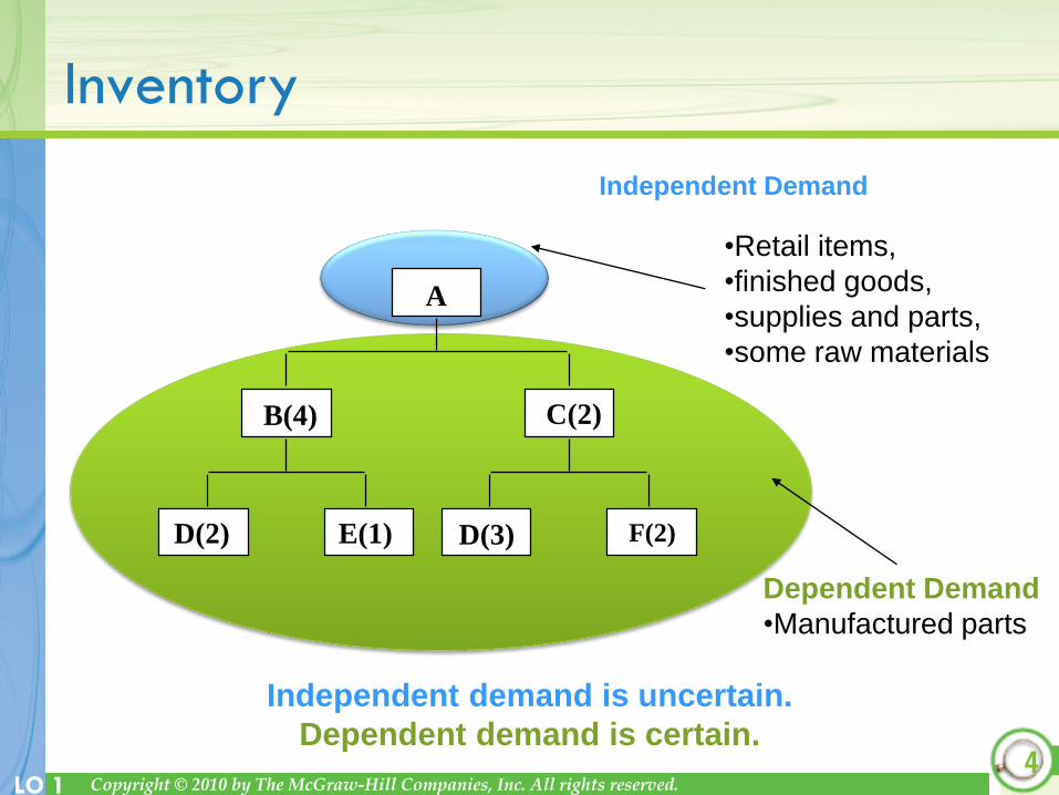
Inventory

•Retail items,

•finished goods,

•supplies and parts,

•some raw materials

A

B(4) C(2)

D(2) E(1) D(3) F(2)

Dependent Demand

•Manufactured parts

Independent demand is uncertain.

Dependent demand is certain.

Independent Demand

4


Safely Storing Inventory

Warehouse Management System (WMS)

computer software that controls the

movement and storage of materials within a warehouse,

and processes the associated transactions

5

Warehouse/storeroom concerns

Security Safety Obsolescence


Inventory Counting Systems

Periodic counting

Physical count of items made

at periodic intervals

6

Perpetual (or continual)

tracking keeps track of

removals from and additions

to inventory continuously,

thus providing current levels

of each item


Inventory Replenishment


An order of a fixed size is placed when the amount on hand drops below a minimum quantity called the reorder point

Two-Bin System

Two containers of inventory; reorder when the first is empty

Bar Code

A number assigned to an item or location, made of a group of vertical bars of different thickness that are readable by a scanner

Universal Product Code (UPC)

Radio Frequency Identification (RFID) technology that uses a RFID tag

attached to the item that emits radio waves to identify items.

0

214800 232087768

7


Forecasting Demand

Lead time

time interval between ordering and receiving the order

Point of Sale (POS) system

Software for electronically recording actual sales at the time and location of sale

8


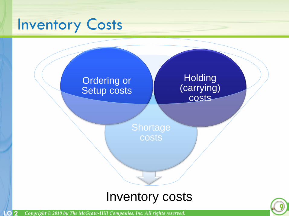
Inventory Costs

Inventory costs

Shortage costs

Ordering or Setup costs

Holding (carrying)

costs

9


Inventory Costs

Holding (carrying) costs

cost to carry an item in inventory

Ordering costs

costs determining order quantity, preparing purchase orders, and fixed cost portion of receiving, inspection, and material handling

Setup costs

Time spent preparing equipment for the job by adjusting machine, changing tools, etc

Shortage costs

costs when demand exceeds supply; often unrealized profit per unit

10


ABC Classification System

Classifying inventory according to some measure of importance and allocating control efforts accordingly.

A - very important

B - mod. important

C - least importantAnnual

$ value

of items

A

B

C

High(70-80)

Low(5-10)

Low(15-20)

High(50-60)

Percentage of Items11

A items

should receive

more attention!


Example: A-B-C Classification

Item

Number

Annual

Demandx

Unit

Cost=

Annual

Dollar

Volume

(ADV)

% of Total

ADV

8 1,000 $ 90.00 $ 90,000 38.8%

10 500 154.00 77,000 33.2%

2 1,550 17.00 26,350 11.3%

5 350 42.86 15,000 6.4%

3 1,000 12.50 12,500 5.4%

1 600 14.17 8,500 3.7%

7 2,000 .60 1,200 .5%

9 100 8.50 850 .4%

6 1,200 .42 504 .2%

4 250 .60 150 .1%12

72%

23%

5%

A

B

C


Cycle Counting

Cycle counting management

How much accuracy is needed?

When kind of counting cycle should be used?

Who should do it?

13

Regular actual count of the items in

inventory on a cyclic schedule


Fixed Order Quantity/Reorder Point Model: Determining Economic Order Quantity

basic economic order quantity (EOQ)

EOQ with

quantity discount

EOQ with

planned shortage

economic production quantity

(EPQ)

14

economic order quantity (EOQ)

The order size that minimizes

total inventory control cost


Assumptions of EOQ Model

1. Only one product is involved

2. Annual demand requirements known

3. Demand is even throughout the year

4. Lead time does not vary

5. Each order is received in a single delivery

6. There are no quantity discounts

7. Shortage is not allowed

15


R = Reorder point

Q = Economic order quantity

LT = Lead time

LT LT

Q QQ

R

Time

Quantity

on hand

1. You receive an order (size = Q)

2. Quantity decreases

by demand rate (d)

3. When quantity reaches reorder

point quantity (R), place another

order (size = Q).

4. Order received after lead time (LT)

expires, when 0 on hand. The cycle

then repeats.

16

Inventory Cycles with EOQ


EOQ: Minimizing Total Costs

Ordering Costs

Holding

Costs

Order Quantity (Q)

ANNUAL

COST

Total Cost

QO

Total cost = Holding + Ordering Costs

Total cost is minimized at Q0 where holding = ordering cost

17


Total

Annual =

Cost

Annual

Ordering

Cost

Annual

Holding

Cost

+TC = Total annual cost

Q = Order quantity (units)

H = Annual holding cost

per unit

D = Annual Demand

S = Ordering (or setup)

cost per order

Q0 = EOQ

18

TCQ

HD

QS

2

Basic Economic Order Quantity (EOQ)

Cost Holding Annual

Cost) Setupor (Order Demand) 2(Annual =

H

2DS = QO


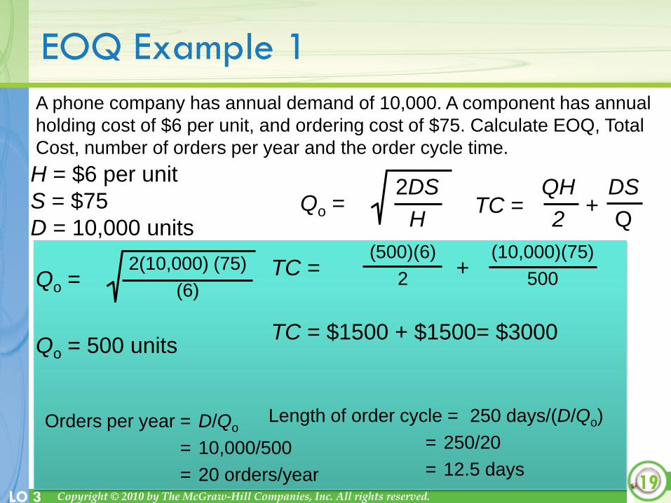
EOQ Example 1

H = $6 per unit

S = $75

D = 10,000 units

Qo =2(10,000) (75)

(6)

Qo = 500 units

TC = +(10,000)(75)

500

(500)(6)

2

TC = $1500 + $1500= $3000

Orders per year = D/Qo

= 10,000/500

= 20 orders/year

Length of order cycle = 250 days/(D/Qo)

= 250/20

= 12.5 days19

Qo =2DS

HTC = +

QH

2

DS

Q

A phone company has annual demand of 10,000. A component has annual

holding cost of $6 per unit, and ordering cost of $75. Calculate EOQ, Total

Cost, number of orders per year and the order cycle time.


Qo =2(15,000) (75)

(6)

Qo = 612 units

TC = +(15,000)(75)

612

(612)(6)

2

TCmin = $1836 + $1838 = $3674

Orders per year = D/Qopt

= 15,000/612

= 25 orders/year

Total cost is 22% more than $3000

EOQ is 22%

more than 500

20

Length of order cycle = 250 days/(D/Qo)

= 250/25

= 10 days

EOQ Example 2a

H = $6 per unit

S = $75

D = 15,000 unitsQo =

2DS

HTC = +

QH

2

DS

Q


holding cost of $6 per unit, and ordering cost of $75. Calculate EOQ, Total

Cost, number of orders per year and the order cycle time.


Qo =2(15,000) (75)

(6)

Qo = 612 units

TC = +(15,000)(75)

500

(500)(6)

2

TC = $1500 + $2250 = $375021

What if we still use

EOQ of 500?

What is total cost?

Total cost is only an extra 2% more if still

use EOQ of 500

EOQ Example 2b

H = $6 per unit

S = $75

D = 15,000 units

Qo =2DS

HTC = +

QH

2

DS

Q


holding cost of $6 per unit, and ordering cost of $75.


Robust Model

The EOQ model is robust

It works even if all parameters

and assumptions are not met

The total cost curve is relatively flat near the

EOQ (especially to the right)

22


Economic Production Quantity (EPQ)

Production done in batches or lots

production capacity > usage or demand rate

for a part for the part

23

Assumptions of EPQ

similar to EOQ

except orders are received

incrementally during production



24



dpp

QI

p

Q

d

Q

SQ

DH

I

max

max

;lengthRun ;length Cycle

2Cost

Setup

Annual

Cost

Holding

Annual

TC

25

dp

p

H

DSQ

20TC = Total annual cost

Q = Order quantity (units)

H = Annual holding cost

per unit

D = Annual Demand

S = Ordering (or setup)

cost per order

Q0 = Optimal run or order quantity

p = Production rate

d = Usage or demand rate

Imax = Maximum inventory level


EPQ Example

Holdit Inc. produces reusable shopping bags. Demand is 20,000 bags per day, 5 days per week, 50 weeks per year. Production is 50,000 per day. The setup cost is $200 and the annual holding cost rate is $.55 per bag. Calculate the EPQ, the total cost, the cycle length and optimal production run length.

H = $0.55 per bag S = $200 D = 20,000 bags x 50 wks x 5 days

d = 20,000 bags per day p = 50,000 bags per day

26

dp

p

H

DSQ

20

850,772050

50

55.

)200)(000,000,5(20

GG

GQ


EPQ Example



27

dpp

QIS

Q

DH

I

max

max 2

TC

bags 46,710 30000000,50

850,77max I

$25,690 002850,77

5)55(.

2

710,46TC

million

Holdit Inc. produces reusable shopping bags. Demand is 20,000 bags per day, 5 days per wk, 50 wks per yr. Production is 50,000 per day. Setup cost is $200 and annual holding cost rate is $.55 per bag. Calculate total cost.


EPQ ExampleHoldit Inc. produces reusable shopping bags. Demand is 20,000 bags per day, 5 days per week, 50 weeks per year. Production is 50,000 per day. The setup cost is $200 and the annual holding cost rate is $.55 per bag. Calculate cycle length and optimal production run length.



28

p

Q

d

Q lengthRun ;length Cycle

days 3.89every 000,20

850,77length Cycle

orderper days 56.1000,50

850,77lengthRun


EOQ with Quantity Discounts

Price reductions are often offered as incentive to buy

larger quantities

Weigh benefits of reduced purchase price against

increased holding cost

R = per unit price of the item

D = annual demand

Annualholdingcost

PurchasingcostTC = +

Q

2H

D

QSTC = +

+Annualorderingcost

RD+


Total Cost with Purchase CostC

ost

EOQ

TC with PD

TC without PD

PD

0 Quantity

Adding Purchasing cost

doesn’t change EOQ

30


Total Cost with Quantity Discounts

31


Best Purchase Quantity Procedure

begin with the lowest unit price

compute the EOQ for each price range

stop when find a feasible EOQ

Is EOQ for the lowest unit price feasible?

Yes: it is the optimal order

quantity

No: compare total cost at all break quantities larger

than feasible EOQ

32

The quantity that yields the

lowest total cost is optimum


Example: Quantity Discounts

Below is a quantity discount schedule for an item with an annual demand of 10,000 units that a company orders regularly at an ordering cost of $4. The annual holding cost is 2% of the purchase price per year. Determine the optimal order quantity.

Order Quantity(units) Price/unit($)

0 to 2,499 $1.20

2,500 to 3,999 1.00

4,000 or more .98

33


units 1,826 = 0.02(1.20)

4)2(10,000)( =

H

2DS = QO

D = 10,000 units S = $4

units 2,000 = 0.02(1.00)

4)2(10,000)( =

H

2DS = QO

units 2,020 = 0.02(0.98)

4)2(10,000)( =

H

2DS = QO

H = .02R R = $1.20, 1.00, 0.98

Interval from 0 to 2499,

the Qo value is feasible

Interval from 2500-3999,

Qo value is NOT feasible

Interval from 4000 & up,

Qo value is NOT feasible

34

Order Quantity Price/unit($)

0 to 2,499 $1.20

2,500 to 3,999 1.00

4,000 or more .98



Quantity Discount Models

2500 4000

An

nu

al

co

st

0 Quantity

EOQs (not feasible)

1st break quantity

2nd break quantity

1st range total cost

curve

35

2nd range total cost curve

3rd range total cost curveEOQ


TC(0-2499) = (1826/2)(0.02*1.20) + (10000/1826)*4+(10000*1.20)

= $12,043.82

TC(2500-3999)= $10,041

TC(4000&more)= $9,949.20

Therefore the optimal order quantity is 4000 units

36


Q

2H

D

QSTC = + RD+


EOQ with Planned Shortages Assumptions:

all shorted demand is back-ordered

back-orders incur shortage costs

shortage cost is proportional to waiting time

all other basic EOQ assumptions

37


EOQ with Planned Shortages

orderper cost setup)(or ordering S

demand annual D

unitper cost holding annual H

cycleorder per ordered-backquantity

yearper unit per cost order back

2

22

Cost

OrderBack

Annual

Cost

Ordering

Annual

Cost

Holding

Annual

TC

22

b

bb

Q

B

B

BH

H

DSQ

BQ

QS

Q

DH

Q

QQTC

38


Example: EOQ with Planned Shortage

Annual demand for a refrigerator is 50 units. Holding cost per unit per year is $200. Back-order cost per unit per year is estimated to be $500.Ordering cost from the manufacturer is $10 per order. Determine order quantity and back-order quantity per order cycle.

39

D = 50 H = $200 B = $500 S = $10

2 2(50)(10) 200 5002.65, round to 3 units.

200

2003 0.86, round to1.

200 500b

DS H BQ

H B B

HQ Q

H B

Allow inventory to drop to zero.

When another unit is demanded, order 3 units.


What’s next?

EOQ models give HOW MANY to order

Now look at WHEN to order

Reorder Point (ROP)

40

d = Demand rate (units per day or week)

LT = Lead time (in days or weeks)

Note: Demand and lead time must have the same time units.

ROP = d LT


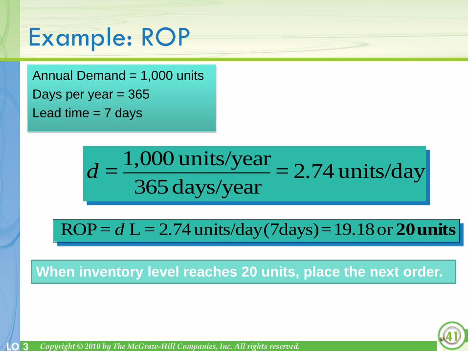
Annual Demand = 1,000 units

Days per year = 365

Lead time = 7 days

units/day 2.74 = days/year 365

units/year 1,000 = d

units 20or 19.18=(7days)units/day 2.74=L =ROP d

When inventory level reaches 20 units, place the next order.

41

Example: ROP



Safety Stock

1. Variability of demand and lead time

2. Service Level

2a. Lead time service level

2b. Annual service level

42

Reorder Point = Expected demand + Safety Stock

(ROP) during lead time


When to Reorder with EOQ Ordering

Reorder Point – When inventory level drops to this amount, the item is reordered.

Safety Stock - Stock that is held in excess of expected demand due to variability of demand and/or lead time.

Service Level – Probability demand will not exceed supply.

Lead time service level: probability that demand will not exceed supply during lead time.

Annual service level: percentage of annual demand filled.

43


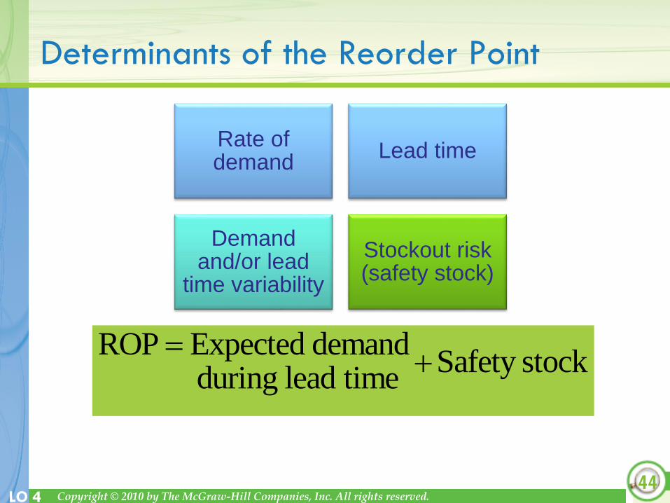
Determinants of the Reorder Point

Rate of demand

Lead time

Demand and/or lead

time variability

Stockout risk (safety stock)

44

ROP Expected demandSafety stock

during lead time


Safety Stock

LT Time

Expected demand

during lead time

Maximum probable demand

during lead time

ROP

Qu

an

tity

Safety stock

Safety stock reduces risk of

stockout during lead time

45


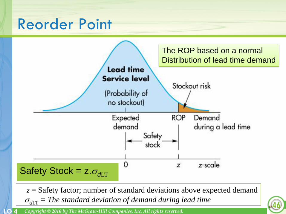
Reorder Point

46

z = Safety factor; number of standard deviations above expected demand

dLT = The standard deviation of demand during lead time

Safety Stock = z.dLT

The ROP based on a normal

Distribution of lead time demand


Demand During Lead Time

47


ROP with Lead Time Service Level

variable demand during a lead time

ROP = expected demand during lead time + safety stock

48

z = Safety factor; number of standard deviations above expected demand

dLT = The standard deviation of demand during lead time

ROP = + z.dLT



variable demand and constant lead time

ROP =

(average demand x lead time) + z x st. dev. of demand during lead time

(demand and lead time measures in same time units)

d = standard deviation of demand per day

dLT = d LT

49



both demand and lead time are variable

ROP =

(avg. demand x avg. lead time) + z x st. dev. of demand in lead time(demand and lead time measures in same time units)

d= standard deviation of demand per day

LT= standard deviation of lead time

dLT = (average lead time x d2)

+ (average daily demand) 2LT2

50


Example 1: ROP with Lead Time Service Level

Calculate the ROP required to achieve a 95% service level

for a product with average demand of 350 units per week and

a standard deviation of demand during lead time of 10. Lead

time averages one week.

From Table 12-3 (p434), z for 95% = 1.65

ROP = 350 + ZdLT

= 350 + 1.65 (10)

= 350 + 16.5 = 366.5 ≈ 367

A new order should be placed when

inventory level reaches 367 units.51



Calculate the ROP and amount of safety stock required to

achieve a 90% service level for a product with variable

demand that averages 15 units per day with a standard

deviation of 5. Lead time is consistently 2 days.

From Table 12-3 (p434), z for 90% = 1.28

ROP = (15 units x 2 days) + ZdLT

= 30 + 1.28 ( 2) (5)

= 30 + 8.96 = 38.96 ≈ 39

Safety stock is about 9 units and

a new order should be placed when

inventory level reaches 39 units.52



Calculate the ROP for a product that has an average demand of

150 units per day and a standard deviation of 16. Lead time

averages 5 days, with a standard deviation of 2. The company

wants no more than 5% stockouts.

service level = 1 – 5% = 95%From Table 12-3 (p434), z for 95% = 1.65

Place a new order when inventory level reaches 1004 units

53

ROP = (150 units x 5 days) + 1.65dlt

= (150 x 5) + 1.65 (5 days x 162) + (1502 x 12)

= 750 + 1.65 (154) = 1,004 units


ROP Using Annual Service Level

1. Calculate

2. Use a table to find the z value associated with E(z)

3. Use the z value in the appropriate ROP formula,

54

dLT

annualSLQzE

)1()(

dLTzROP timeleadduringdemandexpected

SLannual = annual service level

E(z) = standardized expected number of units short during an order cycle.


Min/Max model

similar to fixed order-quantity/reorder point

(ROP) model

difference:

if at order time, Q on hand < min (ROP),

then order quantity = max – Q on hand

(max EOQ + ROP)

55


Inventory Models

EOQ/ROP modelOrder size constant, time between orders changes

Fixed Order Interval/Order up to Level Modelorders placed at fixed time intervals

determine how much to order to bring inventory level up to a predetermined point (order up to level)

used widely for retail

consider expected demand during lead time, safety stock, and amount on hand

demand or lead time can be variable

56


Comparing Inventory Models

57

EOQ/ROP

Fixed

Interval/

Order up to


Disadvantages

requires a larger safety stock

increases carrying cost

costs of periodic reviews

Fixed Order Interval: Benefits and Disadvantages

Benefits

grouping items from same supplier can reduce ordering/shipping costs

practical when inventories cannot be closely monitored

58


Fixed Order Interval/Order up to Level Model

Determining the order interval

59

OI = order interval (in fraction of a year)

S = fixed ordering cost per purchase order

s = variable ordering cost per SKU included in the order (line item)

(assume s is the same for every SKU)

n = n number of SKUs purchased from the supplier

Rj = unit cost of SKUj , j = 1, …, n

i = annual holding cost rate

Dj = annual demand of SKUj , j = 1, …., n

Total Annual Inventory Cost:

TC =

Optimal Order Interval:

OInsSiR

OIDj

j 1)(.

2

.

jjRDi

nsSOI

)(2*


Fixed Order Interval/Order up to Level Model

Determining the Order up to Level

LTOIzLTOId d

Stock

Safety

interval

protection during

demand Expected

I

handon Amount IQ

max

max

60

= Average daily or weekly or monthly demand

OI = Order interval (length of time between orders

LT = Lead time in days or weeks or months

z = Safety factor; # of standard deviations above expected demand

d = Standard deviation of daily or weekly or monthly demand


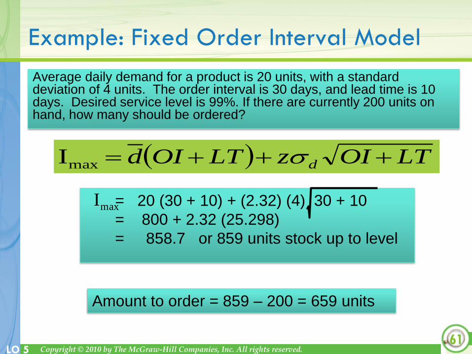
= 20 (30 + 10) + (2.32) (4) 30 + 10

= 800 + 2.32 (25.298)

= 858.7 or 859 units stock up to level

Average daily demand for a product is 20 units, with a standard deviation of 4 units. The order interval is 30 days, and lead time is 10 days. Desired service level is 99%. If there are currently 200 units on hand, how many should be ordered?

61

LTOIzLTOId d maxI

maxI

Amount to order = 859 – 200 = 659 units

Example: Fixed Order Interval Model

week 10

Documents