water waves and ship hydrodynamics: an introduction, second edition
TRANSCRIPT

Water Waves and Ship Hydrodynamics
2nd Edition

A.J. Hermans
Water Wavesand Ship Hydrodynamics
An Introduction
2nd Edition

A.J. HermansTechnical University DelftDelftThe [email protected]
ISBN 978-94-007-0095-6 e-ISBN 978-94-007-0096-3DOI 10.1007/978-94-007-0096-3Springer Dordrecht Heidelberg London New York
Library of Congress Control Number: 2010938437
1st edition: © Delft University, uitgave Martinus Nijhoff Publishers, a member of the Kluwer AcademicPublishers Group, 19852nd edition: © Springer Science+Business Media B.V. 2011No part of this work may be reproduced, stored in a retrieval system, or transmitted in any form or byany means, electronic, mechanical, photocopying, microfilming, recording or otherwise, without writtenpermission from the Publisher, with the exception of any material supplied specifically for the purposeof being entered and executed on a computer system, for exclusive use by the purchaser of the work.
Cover design: eStudio Calamar S.L.
Printed on acid-free paper
Springer is part of Springer Science+Business Media (www.springer.com)

Preface to the Second Edition
This book is a revision and extension of the book published by R. Timman, A.J. Her-mans and G.C. Hsiao based on the lecture notes of courses presented by Timman atthe University of Delaware in 1971 and by Hermans at the Technical University ofDelft. The main topic of the original text is based on linearised free surface waterwave theory. For many years the first edition of the book is used by Aad Hermans asmaterial for a course in ship hydrodynamics presented to Master students in appliedmathematics and naval architecture at the Technical University of Delft. Influencedby the progress in the research in water waves and especially in ship hydrodynamicsthe contents of the course has changed gradually. For instance in offshore engineer-ing the topic like the low-frequency motion of objects moored to a buoy has becomean important issue during this period. Therefore an introduction in this field has beenadded. For didactic reasons the very simple rather abstract problem of the motionof a vertical wall is added. The reason to do so is that most effects that play a rolecan be treated analytically, while for a general three dimensional object some termscan only be obtained numerically. The use of numerical programs is normal practicein this field, therefor an introduction in the theory of integral equations is presentedand some specific problems which may arises, such how to avoid non-physical res-onance at the so called irregular frequencies may be avoided. In the first edition aderivation of the structure of the equations of motion in all six degrees of freedom ispresented. Because the functions derived there are not easily computed in a practicalcase, we restrict ourselves to the derivation of the equation of motion in one degreeof freedom.
A.J. HermansDelft, The Netherlands
v


Preface to the First Edition
In the spring of 1971, Reinier Timman visited the University of Delaware duringwhich time he gave a series of lectures on water waves from which these notesgrew. Those of us privileged to be present during that time will never forget theexperience. Rein Timman is not easily forgotten.
His seemingly inexhaustible energy completely overwhelmed us. Who could for-get the numbing effect of a succession of long wine-filled evenings of lively con-versation on literature, politics, education, you name it, followed early next day bythe appearance of the apparently totally refreshed red-haired giant eager to discussmathematical problems with keen insight and remarkable understanding, ready tolecture on fluid dynamics and optimal control theory or a host of other subjects andready to work into the evening until the cycle repeated. He thought faster, knewmore, drank more and slept less than any of the mortals; he literally wore us out.What a rare privilege indeed to have participated in this intellectual orgy. Timman’slively interest in almost everything coupled with his buoyant enthusiasm and infec-tious optimism epitomised his approach to life, No delicate nibbling at the fringes,he wanted every morsel of every course.
In these times of narrow specialisation, truly renaissance figures are, if not ex-tinct, at least a highly endangered species. But Timman was one of that rare breed.His knowledge in virtually all areas of classical applied mathematics was prodi-gious. I still marvel that while I was his doctoral student in Delft in the late fiftiesworking on a problem in electromagnetic scattering he had at the same time studentsworking in water waves, cavitation, elasticity, aerodynamics and numerical analysis.He was a boundless source of inspiration to his students in all of these varied fields.
His inattention to detail is legendary but this did not hamper his ability to fo-cus on what was really important in a problem. With a wave of his large hand hewould dismiss unimportant errors while concentrating on central ideas, leaving tous the task of setting things right mathematically. This nonchalant attitude towardminus signs and numerical factors was probably deliberate. He wanted people to seethe forest, not the trees; to focus on the heart of the problem, not inconsequentialsuperficialities. He had little use for the all too prevalent penchant for examiningsomeone’s work looking for errors. He would read a paper looking for the gold, notthe dross; looking for what was right, not what was wrong.
vii
viii Preface to the First Edition
Of course this did not make life easy for those around him but it did make itinteresting. This will be attested to by George Hsiao and Richard Weinacht whoserevised version of the notes from Timman’s water wave lectures appeared as a Uni-versity of Delaware report. Timman and Hsiao then planned to further revise andexpand these notes and publish them in book form, but the project came to an abrupthalt with Reinier Timman’s untimely death in 1975. It might have remained unfin-ished had not Aad Hermans’ visit of Delaware in 1980 breathed new life into it.Together George Hsiao and Aad Hermans have completed the task of revising thenotes, reorganising the presentation, restoring the factors of 2 which Timman hadcavalierly omitted, and adding some new material. The first four chapters are basedsubstantially on the original notes, while the fifth chapter and appendices have beenadded.
It is gratifying to see the completion of these notes. It is not unreasonable to hopethat they will provide a useful introduction to water waves for a new generationof mathematicians and engineers. This area was perhaps first among equals in thebroad spectrum of Timman’s interests. If these notes succeed in stimulating a newgeneration to concentrate on the challenging problems remaining in this field, theywill serve a fitting memorial to a remarkable man whose like will not be soon seenagain.
R.E. KleinmanNewark, DelawareMarch, 1985

Acknowledgements to the First Edition
The authors wish to thank Professor Willard E. Baxter for his active interest in thepublication of these lecture notes. We are grateful to Professor Richard J. Weinachtwho spent a great deal of time helping one of us (GCH) in preparing the originaldraft of the water wave notes on which the present first four chapters were based.We owe special debt to Professor Ralph E. Kleinman without whom this projectprobably would never have started.
We would like to express our appreciation to Mr. G. Broere for making most ofthe drawings, and to Mrs. Angelina de Wit for typing the final manuscript.
Finally, we would like to express our gratitude to the Department of Mathemat-ical Sciences of the University of Delaware, the Department of Mathematics andInformatics of the Delft University of Technology and the Alexander von HumboldtStiftung for financial support at various stages of the preparation of this manuscript.
A.J. HermansG.C. Hsiao
March, 1985
ix


Contents
1 Theory of Water Waves . . . . . . . . . . . . . . . . . . . . . . . . . 11.1 Basic Linear Equations . . . . . . . . . . . . . . . . . . . . . . . 11.2 Boundary Conditions . . . . . . . . . . . . . . . . . . . . . . . . 21.3 Linearised Theory . . . . . . . . . . . . . . . . . . . . . . . . . . 4
1.3.1 Small Amplitude Waves in a Steady Current . . . . . . . . 51.3.2 Small Amplitude Waves in a Small Velocity Flow Field . . 7
2 Linear Wave Phenomena . . . . . . . . . . . . . . . . . . . . . . . . . 112.1 Travelling Plane Waves . . . . . . . . . . . . . . . . . . . . . . . 11
2.1.1 Plane Waves . . . . . . . . . . . . . . . . . . . . . . . . . 112.1.2 Wave Energy Transport . . . . . . . . . . . . . . . . . . . 14
2.2 Cylindrical Waves . . . . . . . . . . . . . . . . . . . . . . . . . . 182.3 Harmonic Source Singularity . . . . . . . . . . . . . . . . . . . . 202.4 The Moving Pressure Point . . . . . . . . . . . . . . . . . . . . . 272.5 Wave Fronts . . . . . . . . . . . . . . . . . . . . . . . . . . . . . 292.6 Wave Patterns . . . . . . . . . . . . . . . . . . . . . . . . . . . . 312.7 Singularity in a Steady Current . . . . . . . . . . . . . . . . . . . 35
2.7.1 Steady Singularity . . . . . . . . . . . . . . . . . . . . . . 352.7.2 Oscillating Singularity . . . . . . . . . . . . . . . . . . . . 38
3 Boundary Integral Formulation and Ship Motions . . . . . . . . . . 413.1 Scattering of Acoustic Waves . . . . . . . . . . . . . . . . . . . . 41
3.1.1 Direct Method . . . . . . . . . . . . . . . . . . . . . . . . 443.1.2 Source Distribution . . . . . . . . . . . . . . . . . . . . . 45
3.2 Scattering of Free Surface Waves . . . . . . . . . . . . . . . . . . 463.2.1 Fixed Object . . . . . . . . . . . . . . . . . . . . . . . . . 473.2.2 Direct Method . . . . . . . . . . . . . . . . . . . . . . . . 493.2.3 Source Distribution . . . . . . . . . . . . . . . . . . . . . 493.2.4 Motions of a Floating Object, Ship Motions . . . . . . . . 503.2.5 Heave Motion of a Floating Object . . . . . . . . . . . . . 53
3.3 Slow Speed Approximation . . . . . . . . . . . . . . . . . . . . . 56
xi

xii Contents
4 Second-Order Theory . . . . . . . . . . . . . . . . . . . . . . . . . . 594.1 Second-Order Wave Theory . . . . . . . . . . . . . . . . . . . . . 594.2 Wave-Drift Forces and Moments . . . . . . . . . . . . . . . . . . 62
4.2.1 Constant and Low Frequency Drift Forces by Means ofLocal Expansions . . . . . . . . . . . . . . . . . . . . . . 63
4.2.2 Constant Drift Forces by Means of Far-Field Expansions . . 654.3 Demonstration of Second-Order Effects, a Classroom Example . . 69
4.3.1 Interaction of Waves with a Vertical Wall . . . . . . . . . . 694.3.2 Forces on a Fixed Wall . . . . . . . . . . . . . . . . . . . 714.3.3 Moving Wall . . . . . . . . . . . . . . . . . . . . . . . . . 724.3.4 First-Order Motion of the Wall . . . . . . . . . . . . . . . 734.3.5 Influence of the Motion on the Low Frequency Drift Force . 774.3.6 Second-Order Motion of the Wall . . . . . . . . . . . . . . 774.3.7 Some Observations . . . . . . . . . . . . . . . . . . . . . 78
5 Asymptotic Formulation . . . . . . . . . . . . . . . . . . . . . . . . . 795.1 Thin Ship Hydrodynamics, Michell Theory . . . . . . . . . . . . . 795.2 Short Wave Diffraction by a Sailing Ship . . . . . . . . . . . . . . 82
6 Flexible Floating Platform . . . . . . . . . . . . . . . . . . . . . . . . 876.1 The Finite Draft Problem . . . . . . . . . . . . . . . . . . . . . . 886.2 Semi-Analytic Solution . . . . . . . . . . . . . . . . . . . . . . . 91
6.2.1 Semi-Infinite Platform . . . . . . . . . . . . . . . . . . . . 936.2.2 Strip of Finite Length . . . . . . . . . . . . . . . . . . . . 96
7 Irregular and Non-linear Waves . . . . . . . . . . . . . . . . . . . . . 1037.1 Wiener Spectrum . . . . . . . . . . . . . . . . . . . . . . . . . . . 1037.2 Shallow Water Theory . . . . . . . . . . . . . . . . . . . . . . . . 1097.3 Non-linear Dispersive Waves . . . . . . . . . . . . . . . . . . . . 114
8 Shallow Water Ship Hydrodynamics . . . . . . . . . . . . . . . . . . 1258.1 Thin Airfoil Theory . . . . . . . . . . . . . . . . . . . . . . . . . 1258.2 Slender Body Theory . . . . . . . . . . . . . . . . . . . . . . . . 1338.3 Free Surface Effects . . . . . . . . . . . . . . . . . . . . . . . . . 1378.4 Ships in a Channel . . . . . . . . . . . . . . . . . . . . . . . . . . 1468.5 Interaction of Ships . . . . . . . . . . . . . . . . . . . . . . . . . 151
9 Appendices: Mathematical Methods . . . . . . . . . . . . . . . . . . 1559.1 The Method of Stationary Phase . . . . . . . . . . . . . . . . . . . 1559.2 The Method of Characteristics . . . . . . . . . . . . . . . . . . . . 1599.3 Singular Integral Equations . . . . . . . . . . . . . . . . . . . . . 1619.4 The Two-Dimensional Green’s Function . . . . . . . . . . . . . . 1629.5 Simplification of the Set of Algebraic Equations . . . . . . . . . . 163
References . . . . . . . . . . . . . . . . . . . . . . . . . . . . . . . . . . . 165
Index . . . . . . . . . . . . . . . . . . . . . . . . . . . . . . . . . . . . . . 167

Chapter 1Theory of Water Waves
This chapter contains the formulation of boundary and initial boundary value prob-lems in water waves. The basic equations here are the Euler equations and theequation of continuity for a non-viscous incompressible fluid moving under gravity.Throughout the book, in most considerations the motion is assumed to be irrota-tional and hence the existence of a velocity potential function is ensured in simplyconnected regions. In this case the equation of continuity for the velocity of the fluidis then reduced to the familiar Laplace equation for the velocity potential function.
Water waves are created normally by the presence of a free surface along whichthe pressure is constant. For the irrotational motion, on the free surface one thanobtains the non-linear Bernoulli equation for the velocity potential function fromthe Euler equation. Based on small amplitude waves, linearised problems for thevelocity potential function and for the free surface elevation are formulated.
At first we follow the derivation as can be found in [17, 19] to obtain equationsfor the wave potential in still water and as a superposition on a constant parallelflow potential. The coefficients in the free surface equations are constant. Then wederive linear equation for the superposition of small amplitude waves on a flowdisturbed by some three dimensional object. If we consider the magnitude of thesteady velocity vector to be small, we obtain for the time-dependent wave potentialfunction a linear equation with non-constant coefficients.
1.1 Basic Linear Equations
The theory of water waves, to be presented here, is based on a model of non-viscousincompressible fluid moving under gravity. The equations of motion will be ex-pressed in a right-handed system of rectangular coordinates x, y, z. In the Eulerrepresentation they read
ut + uux + vuy + wuz = − 1
ρpx,
A.J. Hermans, Water Waves and Ship Hydrodynamics,DOI 10.1007/978-94-007-0096-3_1, © Springer Science+Business Media B.V. 2011
1
2 1 Theory of Water Waves
vt + uvx + vvy + wvz = − 1
ρpy − g, (1.1)
wt + uwx + vwy + wwz = − 1
ρpz.
Here u = u(x, y, z, t), v = v(x, y, z, t),w = w(x,y, z, t) are velocity componentsin the corresponding x, y, z direction; p = p(x, y, z, t) is the pressure; ρ is the den-sity of the fluid, a constant, and g is the gravitational acceleration. The continuityequation is
ux + vy + wz = 0. (1.2)
In most of the considerations the fluid motion is considered to be irrotational. Thisgives the additional set of equations
uy − vx = 0,
vz − wy = 0,
wx − uz = 0,
(1.3)
which guarantees in a simply connected region the existence of a velocity potentialϕ with
u = ϕx,
v = ϕy,
w = ϕz.
(1.4)
From (1.2) we see that ϕ satisfies Laplace’s equation,
ϕxx + ϕyy + ϕzz = 0. (1.5)
This greatly facilitates the theory.In general, however, solutions of Laplace’s equation will not show wave charac-
ter, since the equation is elliptic. Waves are created by the presence of a free surfaceand are intimately related to the free surface condition.
1.2 Boundary Conditions
At the moving boundary the condition for a non-viscous fluid is very simple. Thefluid velocity normal to the surface has to be equal to the normal component of thevelocity of the surface itself. If the equation of the surface is given by
y = F(x, z, t), (1.6)

1.2 Boundary Conditions 3
we denote the velocity of a point on the surface by (U,V,W). A normal to thesurface has the direction cosines(
Fx√F 2
x + F 2z + 1
,−1√
F 2x + F 2
z + 1,
Fz√F 2
x + F 2z + 1
)(1.7)
and the surface (or boundary) condition reads
uFx − v + wFz√F 2
x + F 2z + 1
= UFx − V + WFz√F 2
x + F 2z + 1
= −Ft√F 2
x + F 2z + 1
, (1.8)
because
FxU − V + FzW + Ft = 0
for a point on the moving surface. Hence from (1.8) we have
v = Ft + uFx + wFz = dF(x, z, t)
dt, (1.9)
which expresses the fact that, once a fluid particle is on the surface, it remains onthe surface.
We will usually denote the bottom surface by y = H(x, z, t), so that (1.9) reads
v = Ht + uHx + wHz. (1.10)
Mostly in our considerations the bottom is fixed, that is H is independent of t , sothat the term Ht in (1.10) vanishes.
The waves are created at the free surface, which is characterised by the conditionthat along this surface the pressure is a constant. Hence in addition to the kinematicequation
v = ηt + uηx + wηz, (1.11)
for the free surface y = η(x, z, t), we have the condition
p = constant, (1.12)
along y = η(x, z, t). There are two ways of formulating these conditions:
a. From the equations of motion (1.2), we find by inspection, in the case of irrota-tional motion, the Bernoulli equation
ϕt + 1
2(u2 + v2 + w2) + gy + p
ρ= f (t) (1.13)
in which, because of the constant pressure, one can normalise ϕ to result in thedynamical free surface condition
ϕt + 1
2(ϕ2
x + ϕ2y + ϕ2
z ) + gη = constant. (1.14)

4 1 Theory of Water Waves
b. The second way expresses that
∂p
∂sx= 0,
∂p
∂sz= 0, (1.15)
where sx and sz are coordinates on the free surface, which have their projectionsin the x and z directions, respectively. This gives1
∂p
∂sx= ∂p
∂xcos (x, sx) + ∂p
∂ycos (y, sx) = 0,
∂p
∂sz= ∂p
∂zcos (z, sz) + ∂p
∂ycos (y, sz) = 0
(1.16)
or
px + pyηx = 0,
pz + pyηz = 0.(1.17)
Substituting (1.17) into (1.2), we have the relation
ut + uux + vuy + wuz + ηx(vt + uvx + vvy + wvz) = 0,
wt + uwx + vwy + wwz + ηz(vt + uvx + vvy + wvz) = 0,(1.18)
which are also valid for rotational flow.
In this way the basic equations are derived. The further development of the theoryis based on small parameter expansions of these equations. To do so an appropriatesmall dimensionless parameter has to be specified. Depending on the case consid-ered, different formulations arise. In the next section we consider the case of a fixedbottom and where the water region is horizontally extended to infinity while nofloating objects are present. This simplifies the theory considerably. Later we takeother effects into account as well.
1.3 Linearised Theory
In this section we discuss two different cases, where we may obtain linearised equa-tions for different situations. In the first one we assume that the waves are superim-posed on a steady constant parallel flow field (current), while the second one dealswith a wave field superimposed on a steady flow field, which obeys a simplified freesurface condition. This steady flow may be generated by a slowly moving vessel.For fast moving objects one may need a more general non-linear theory for steadyand unsteady boundary conditions. We will deal with some of these problems infuture chapters.
1Note that cos (x, sz) = cos (z, sx) = 0.

1.3 Linearised Theory 5
1.3.1 Small Amplitude Waves in a Steady Current
The simplest approximation is the case where the deviation η of the free surfaceabove a certain standard level, which is taken as y = 0, is small. We assume that
η(x, z, t) = εη(x, z, t), (1.19)
where ε is a small dimensionless parameter. In addition we assume the bottom slopeto be small of the same order of magnitude in ε and put
y = −h + εh1, (1.20)
which will lead to the boundary condition
v = ε(h1t + uh1x + wh1z) (1.21)
from (1.10). For the free surface we obtain from (1.11) and (1.14)
v = ε(ηt + uηx + wηz) (1.22)
together with
ϕt + 1
2(ϕ2
x + ϕ2y + ϕ2
z ) + εgη = constant. (1.23)
Now, for the solution of (1.5), we assume an expansion
ϕ(x, y, z, t) = ϕ0 + εϕ1 + ε2ϕ2 + · · · , (1.24)
and substitute it in (1.5) and boundary condition (1.21). Equating to zero the coeffi-cients of like powers of ε, we get first that all ϕk’s are harmonic functions. Moreover,we have from (1.20) and (1.21)
v0 = ϕ0y = 0,
v1 = h1t + u0h1x + w0h1z,at y = −h. (1.25)
Similarly, we expand η in (1.19) in the form
η = η1 + εη2 + ε2η2 + · · · , (1.26)
and find from (1.22) the free surface condition at y = εη,
v0 = 0 and
v1 = η1t + u0η1x + w0η1z
(1.27)
together with
ϕ0t + 1
2(ϕ2
0x + ϕ20y + ϕ2
0z) = constant,
ϕ1t + u0u1 + v0v1 + w0w1 + gη1 = 0(1.28)
from (1.23).

6 1 Theory of Water Waves
The first approximation ϕ0, u0 = ϕ0x, v0 = ϕ0y,w0 = ϕ0z, corresponds to a per-manent flow. If we take the special case
u0 = constant,
v0 = 0,
w0 = constant,
we can transform to a coordinate system with the x-axis in the direction of this con-stant flow and denote the velocity by U . In this case we have ϕ0 = Ux and the con-stant in (1.23) is equal to 1
2U2. Then we have the boundary condition from (1.25),
v1 = Uh1x at y = −h, (1.29)
and at the free surface y = εη, the coefficient of ε for (1.27) and (1.28) gives
ϕ1y = η1t + Uη1x,
ϕ1t + Uϕ1x + gη1 = 0.(1.30)
Instead of putting this condition (1.30) at y = εη, we put it at y = 0. Assuming thatϕ1 admits an expansion in powers of εη, we then have
ϕ1x(x, εη, z) = ϕ1x(x,0, z) + εηϕ1xy(x,0, z) + · · ·= ϕ1x(x,0, z) + εη1ϕ1xy(x,0, z) + O(ε2),
which leads to a modification of the terms of second order or higher. Hence the firstapproximation gives the following set of linear equations for ϕ1 and η1:
ϕ1xx + ϕ1yy + ϕ1zz = 0,
ϕ1y = h1t + Uh1x at y = −h,
ϕ1y = η1t + Uη1x
ϕ1t + Uϕ1x + gη1 = 0
}at y = 0.
(1.31)
For a fixed flat bottom, h1 is constant so that h1x = h1t = 0. For smooth functions,one can easily eliminate η1 in the surface condition and obtain the formulation forthe first-order approximation (dropping subscript 1):
ϕxx + ϕyy + ϕzz = 0,
ϕy = 0 at y = −h,
U2ϕxx + 2Uϕxt + ϕtt + gϕy = 0 at y = 0.
(1.32)
Here the surface elevation η can be computed by
η = −1
g(ϕt + Uϕx) . (1.33)

1.3 Linearised Theory 7
Now given initial conditions, problems defined by (1.32) can be solved by meansof the Laplace or Fourier transform method. As for illustration, we shall consider afew simple examples in Chap. 2.
1.3.2 Small Amplitude Waves in a Small Velocity Flow Field
Here we derive a free surface for unsteady waves superimposed on the steady freesurface generated by a steady velocity field. This steady field may be generatedby an object positioned in a constant parallel flow field. In general this leads to avery complicated condition, however if the magnitude of the velocity is small it canbe simplified significantly. If no waves are present the magnitude of the velocityis characterised by a small non-dimensional Froude number F = U√
gL, where L
is some length scale that plays a role in the problem, for instance the length ofthe disturbing object. It is assumed that this Froude number is small. In Sect. 5.2we consider the diffraction of short waves if the steady flow field is generated by aparallel flow and is disturbed by a blunt object such as a sphere or a circular cylinder.In these cases we take for L the radius of the sphere or cylinder. Here we derive thefree surface condition for such a case.
The easiest way is to follow the derivation, presented in Sect. 1.3.1, to determinea useful formulation for the steady potential. In this case of constant water depththe only small parameter is the Froude number F = U√
gL. Again we assume that the
deviation of the free surface around y = 0 will be small. However we can not saythat the free surface elevation is of O(F ). The order of magnitude of the elevationfollows from the derivation and will turn out to be O(F 2). For the steady case thekinematic free surface condition (1.11) becomes
v = uηx + wηz. (1.34)
We assume that u,v and w are of the same order of magnitude O(F ). Hence forsmall values of η the kinematic condition reduces to
v = 0 at y = 0. (1.35)
The dynamic free surface condition now determines the order of magnitude of thecorresponding free surface elevation. If we assume that in the far field the potentialequals the unperturbed parallel flow Ux we obtain
η = −1
2g(u2 + v2 + w2 − U2). (1.36)
Because of the specific form of the free surface condition (1.35) the steady potentialdescribed here is called the double body potential. For this potential we use thenotation ϕr , the velocity components are written as (ur , vr ,wr) = ∇ϕr and the freesurface elevation as ηr . If one is interested in the total steady potential one must

8 1 Theory of Water Waves
derive an appropriate free surface condition also describing the wavy pattern. Thiswill be done in Sect. 2.4. Our goal here is to derive a linearised free surface conditionfor the unsteady wave potential.
We assume that the potential ϕ can be decomposed as follows:
ϕ(x, y, z, t) = ϕr(x, y, z) + ϕ0(x, y, z) + ϕw(x, y, z, t). (1.37)
The potential ϕ0 describes the steady wave pattern if waves are not present. Laterwe will show that this potential ϕ0 = o(ϕr), while as we have seen ϕr = O(F ). Forthis reason we neglect this term in the low Froude number small wave expansionand write
ϕ(x, y, z, t) = ϕr(x, y, z) + ϕw(x, y, z, t). (1.38)
The free surface elevation η(x, z, t) is assumed to be of the form
η(x, z, t) = ηr(x, z) + η0(x, z) + ηw(x, z, t). (1.39)
The function η0 = o(ηr ), while ηr = O(F 2), so we neglect η0 and write
η(x, z, t) = ηr(x, z) + ηw(x, z, t). (1.40)
We assume that the elevation of the free surface above the level y = ηr(x, z) issmall O(ε). The condition for the wave potential at the bottom remains the same asbefore, however the free surface condition changes significantly. In principle the twosmall parameters are independent of each other. If the small Froude number is largecompared with ε, we may introduce a new coordinate system (x′, y′ −ηr(x
′, z′), z′).The additional terms in the Laplace equation are small and may be neglected. Theadditional terms in the free surface condition may be neglected as well. If the twoparameters are of the same order of magnitude we may linearise with respect toy = 0 directly, else it is defined at y = ηr . The kinematic condition as in (1.27),becomes
vw = ηwt + urηwx + wrηwz, (1.41)
and if we use the surface condition the dynamic condition becomes
ϕwt + urϕwx + wrϕwz + gηw = 0. (1.42)
We eliminate ηw by means of differentiation of (1.42) with respect to t, x and z
respectively. The additional terms due to differentiation along the double body freesurface ηr are O(F 3) and may be neglected. For the wave potential we obtain thefollowing formulation (we omit the primes):
ϕwxx + ϕwyy + ϕwzz = 0,
ϕwy = 0 at y = −h,
(∂
∂t+ ur
∂
∂x+ wr
∂
∂z
)2
ϕw + g∂ϕw
∂y= 0 at y = 0.
(1.43)

1.3 Linearised Theory 9
The coefficients in the free surface condition depend on the local velocity. Althoughthe formulation for the wave potential is linear, no simple solutions for a wave pat-tern can be given. In the case of the diffraction of short wave by a smooth objectwe will use an asymptotic wave theory. This method is developed in acoustic andelectromagnetic theory, it is generally called the ray method. In Chap. 5 we presentthis asymptotic method.


Chapter 2Linear Wave Phenomena
A few simple examples of the linearised boundary and initial-boundary value prob-lems formulated in the previous chapter will be solved by the Fourier or Laplacetransform method. Through these simple examples, basic wave phenomena or ter-minologies in water waves will be introduced. These are phase velocity, dispersionrelation, group velocity, wave fronts, to name a few.
Of particular importance is the asymptotic behaviour of the free surface elevationfor large values of relevant spaces and for time variables. This behaviour can bebest obtained by the method of stationary phase (see Sect. 9.1). In this connection,the method of characteristics for treating first-order non-linear partial differentialequations for the phase function is employed. Hence a brief summary of the conceptof characteristics is included in Sect. 9.2.
A systematic derivation of oscillatory source singularity functions is presentedfor the disturbance below the free surface with and without current in Sects. 2.3and 2.7.2. In Sect. 2.4 we derive for the steady case the field for a pressure distur-bance at the free surface and for a point source below the free surface in Sect. 2.7.1.These source functions are often called Green functions and are used in numericalcodes. One may derive different formulations for the functions as is shown.
2.1 Travelling Plane Waves
2.1.1 Plane Waves
It is easy to obtain travelling plane waves. As in Chap. 1 for small amplitude wavesthe linearised problem is defined by (1.32). For simplicity we restrict ourselves tothe situation where U = 0. We consider two cases according to the water depth. Webegin with the infinite depth. In this case the boundary value problem (1.32) consistsof the Laplace equation
ϕxx + ϕyy + ϕzz = 0 (2.1)
A.J. Hermans, Water Waves and Ship Hydrodynamics,DOI 10.1007/978-94-007-0096-3_2, © Springer Science+Business Media B.V. 2011
11

12 2 Linear Wave Phenomena
together with the surface conditions
ϕtt + gϕy = 0 at y = 0 (2.2)
and the condition at infinity
ϕy → 0 as y → −∞. (2.3)
We seek a solution ϕ(x, y, z, t) of (2.1)–(2.3) in the form
ϕ(x, y, z, t) = Aei(αx+βz)+ky+iωt , (2.4)
where α,β, k,ω and A are constants. Clearly (2.3) will be satisfied if k is positive.Substituting (2.4) into (2.1) and (2.2) we obtain
k = α2 + β2 and − ω2 + gk = 0. (2.5)
Set α = −k cos θ and β = −k sin θ which clearly satisfy the first equation of (2.5)
for any k. The second one gives that k = ω2
gwhich is known as the dispersion
relation—a relation between wave number k and frequency ω. Then the potentialfunction has the form
ϕ(x, y, z, t) = A exp
{−iω
[ω
g(x cos θ + z sin θ) − t
]+ ω2
gy
}, (2.6)
and consequently the water height is given by
η(x, z, t) = − 1
gϕt = −A
iω
gexp
{−iω
[ω
g(x cos θ + z sin θ) − t
]}(2.7)
through use of (1.33). This formula represents plane waves.For θ = 0, we have plane waves travelling along the x-axis, independent of the
z-coordinate:
η(x, t) = − iω
gAe−i( ω2
gx−ωt) = A1e−i ω2
g(x−ct)
, (2.8)
where c = gω
is the velocity of the wave (or phase velocity) and A1 = − iωg
A is theamplitude of the wave. The real part of (2.8) corresponds to the real values waveheight.
We now consider a wave train consisting of two plane waves in the x-directionwith slightly different frequencies ω and ω + δω. The total wave height may bewritten as
η(x, t) = A1 cos(kx − ωt) + A2 cos((k + δk)x − (ω + δω)t
= A(x, t) cos(kx − ωt + θ(x, t))), (2.9)

2.1 Travelling Plane Waves 13
where the amplitude function A(x, t) and the phase function θ(x, t) are slowly vary-ing functions. They can be written as
A(x, t) =√
A21 + A2
2 + 2A1A2 cos(δkx − δωt) and
tan θ(x, t) = A2 sin(δkx − δωt)
A1 + A2 cos(δkx − δωt).
(2.10)
The amplitude moves with the velocity δωδk
. It will be shown in Sect. 2.1.2 that thewave energy is proportional to the square of the amplitude, hence we may expectthat the energy moves with a velocity
cg = limδω→0
δω
δk= dω
dk. (2.11)
This velocity cg is called the group velocity.The corresponding problem for finite water depth can be treated in the same way.
We write
ϕ(x, y, z, t) = ϕ(x, y, z)eiωt .
Then in this case we have from (2.2) the surface condition
ϕy = ω2
gϕ at y = 0, (2.12)
while the condition at infinity (2.3) is replaced by the boundary condition (1.32). Interms of ϕ we have
ϕy = 0 at y = −h. (2.13)
For travelling waves in the direction of the x-axis, i.e., ϕ = ϕ(x, y), a simple ma-nipulation by the method of separation of variables leads to the solution
ϕ(x, y, t) = A cosh[k(y + h)]e−i(kx−ωt), (2.14)
where the wave number k and the frequency ω are related by the dispersion relation
ω2 = gk tanh(kh). (2.15)
Waves with a different wave number travel with a different phase velocity c whichis defined by
c = ω
k=
√g tanh(kh)
k. (2.16)
Note that for kh small, since tanh(kh) = kh + O((kh)3), we have c = √gh which
is the case without dispersion. Observe again that if we let h → ∞, we recoverthe case of infinite depth, (2.5). The dispersion causes a wave pattern, which at acertain place x and time t is a superposition of harmonic waves to be distorted atother places, because the components travel with different velocities. In the case ofdispersion, it is difficult to determine the concept of ‘wave speed’.

14 2 Linear Wave Phenomena
2.1.2 Wave Energy Transport
For the description of plane waves it is sufficient to restrict the considerations tothe one-dimensional case. We represent at t = 0 the water height η(x,0) by the realintegral
η(x) =∫ ∞
0C(k) cos(kx)dk +
∫ ∞
0S(k) sin(kx)dk (2.17)
with
C(k) = 1
π
∫ ∞
0η(x) cos(kx)dx, and
S(k) = 1
π
∫ ∞
0η(x) sin(kx)dx.
Since C(k) and S(k) are respectively even and odd functions, setting
A(k) = 1
2(C(k) + iS(k)), (2.18)
we can rewrite η(x) as a complex integral
η(x) =∫ ∞
−∞A(k)e−ikx dk. (2.19)
A simple calculation shows that
η(x) = 2�∫ ∞
0A(k)e−ikx dk =
∫ ∞
−∞A∗(k)eikx dk, (2.20)
where A∗(k) is the complex conjugate of A(k).For an understanding of the wave dispersion phenomenon, it is necessary to con-
sider the energy propagation in the wave (linearised approximation). If the functionη(x) belongs to L2, i.e.,
∫ ∞−∞ η(x)2 dx exists, the potential energy is given by
E = 1
2ρg
∫ ∞
−∞η(x)2 dx = 1
2
∫ ∞
−∞
(∫ ∞
−∞A(k)e−ikx dk
)(∫ ∞
−∞A∗(k′)eik′x dk′
)dx
from (2.19) and (2.20). The latter integral can now be calculated by making use ofthe Fourier inversion theorem and the fact that
∫ ∞−∞ ei(k′−k)x dx = 2πδ(k′ − k).
This gives
E = 1
2ρg2π
∫ ∞
−∞|A(k)|2 dk. (2.21)
Hence from (2.18) we have
E = ρgπ
4
∫ ∞
−∞{C(k)2 + S(k)2}dk. (2.22)

2.1 Travelling Plane Waves 15
If the dispersion relation ω = ω(k) is known (for convenience we extend the defini-tion of ω(−k) = −ω(k)), then we can compute the water height η at any arbitrarytime t as follows:
η(x, t) =∫ ∞
−∞A(k)ei(ωt−kx) dk =
∫ ∞
−∞A(k)e−i(ωt−kx) dk (2.23)
in terms of the phase velocity c = ω/k. Here it is assumed that the initial conditionsare such that the wave propagates only in the projection of the positive x-axis.
The total potential energy is conserved; the wave only changes the distributionof the energy along the x-axis. In fact we have
E(t) = 1
2ρg
∫ ∞
−∞|η(x, t)|2 dx
= 1
2ρg
∫ ∞
−∞dx
(∫ ∞
−∞A(k)ei(ωt−kx) dk
)(∫ ∞
−∞A∗(k′)e−i(ω′t−k′x) dk′
)
with ω′ = ω(k′). The latter integral follows from (2.23) and can be calculated simi-larly according to the Fourier inversion theorem. We find again
E(t) = ρgπ
∫ ∞
−∞|A(k)|2 dk. (2.24)
Now we are going to find a measure for the velocity of the energy propagation andcalculate to this end the location of the centre of gravity x(t) of the first moment ofthe energy, which is defined by
x(t) =∫ ∞−∞ x|η(x, t)|2 dx∫ ∞−∞ |η(x, t)|2 dx
, (2.25)
provided both integrals exist. Here the denominator has been shown to be a constantin time and can be calculated easily from (2.24). The numerator, however, requiressome investigation. Equation (2.23) yields
∫ ∞
−∞x|η(x, t)2|dx
=∫ ∞
−∞x dx
∫ ∞
−∞A(k)ei(ωt−kx) dk
∫ ∞
−∞A∗(k′)e−i(ω′t−k′x) dk′
= i∫ ∞
−∞dx
∫ ∞
−∞A(k)d
(ei(ωt−kx)
)∫ ∞
−∞A∗(k′)e−i(ω′t−k′x) dk′
+ t
∫ ∞
−∞dx
∫ ∞
−∞A(k)
dω(k)
dk
∫ ∞
−∞A∗(k′)ei(ωt−kx)−i(ω′t−k′x) dk dk′
:= J1 + J2.

16 2 Linear Wave Phenomena
Integrating by parts and taking account the fact that A(k) → 0, as k → ±∞ in viewof Bessel’s inequality, we find
J1 = −i∫ ∞
−∞dx
∫ ∞
−∞dA(k)
dk
∫ ∞
−∞A∗(k′)ei(ωt−kx)−i(ω′t−k′x) dk dk′.
Then by the Fourier inversion formula, we obtain
J1 = −2π i∫ ∞
−∞dA(k)
dkA∗(k)dk;
J2 = 2πt
∫ ∞
−∞dω(k)
dk|A(k)|2 dk.
Adding J1 and J2, we have∫ ∞
−∞x|η(x, t)2|dx = 2π
{−i
∫ ∞
−∞dA(k)
dkA∗(k)dk + t
∫ ∞
−∞dω(k)
dk|A(k)|2 dk
}.
(2.26)We define, as a mean value of a quantity ψ(k) in the k-domain,
ψ =∫ ∞−∞ ψ(k)|A(k)|2 dk∫ ∞
−∞ |A(k)|2 dk, (2.27)
and remark that the first term in (2.26) determines the position of x(t) for t = 0.Hence we find
x(t) = x(0) + tdω
dk, (2.28)
i.e. the centre of gravity propagates with a velocity which is equal to the meanvelocity of dω
dk. Here dω
dkis called the group velocity; hence the mean value of the
group velocity dωdk
is a measure for the speed of propagation of the energy.The significance of this result becomes clear when we consider an amplitude
spectrum A(k), which extends only over a narrow wave number band:
η(x, t) =∫ k0+ε
k0−ε
A(k)e−i(kx−ω(k)t dk ε > 0. (2.29)
The centre of gravity satisfies
x(t; k0, ε) = x(0; k0, ε) + tω′(k0, ε), (2.30)
where ω′(k0, ε) is now the mean value of ω′(k) = dωdk
over the narrow band[k0 − ε, k0 + ε]. For small values of ε we simply replace ω′(k0, ε) by ω′(k0).
For small values of t , one can make a more accurate analysis of the motion asfollows. Expanding ω(k) in the form
ω(k) = ω(k0) + (k − k0)ω′(k0) + (k − k0)
2
2ω′′(k),

2.1 Travelling Plane Waves 17
and substituting into (2.29), we may write
η(x, t) =∫ k0+ε
k0−ε
A(k)e−i{(k0x−ω(k0)t)+(k−k0)(x−ω′(k0)t)− (k−k0)2
2 ω′′(k)t} dk
= e−i(k0x−ω(k0)t)
∫ k0+ε
k0−ε
A(k)e−i(k−k0)(x−ω′(k0)t) dk + R, (2.31)
where
R = e−i(k0x−ω(k0)t)
∫ k0+ε
k0−ε
A(k)e−i(x−ω′(k0)t)(k−k0)
·{
exp
[i(k − k0)
2
2ω′′(k)t
]− 1
}dk.
Using the inequality |eiu − 1| ≤ |u|, we find an estimate of the remainder
|R| ≤∫ k0+ε
k0−ε
|A(k)| (k − k0)2
2|ω′′(k)t |dk
≤ 1
3
(max|k−k0|<ε
|A(k)|)(
max|k−k0|<ε|ω′′(k)|
)ε3t,
which shows that for not too large values of t , the first term of (2.30) gives a goodapproximation of η. Assuming, for small ε, A(k) to be constant A(k0) over theinterval, we can integrate:
A(k0)e−i(k0x−ω(k0)t)
∫ k0+ε
k0−ε
e−i(k−k0)(x−ω′(k0)t) dk
= A(k0)e−ik0(x− ω(k0)
k0t) 2 sin[(x − ω′(k0)t)ε]
x − ω′(k0)t.
Fig. 2.1 Wave train

18 2 Linear Wave Phenomena
Hence we have, for small ε and t not too large,
η(x, t) ∼= A(k0)e−ik0(x− ω(k0)
k0t) 2 sin[(x − ω′(k0)t)ε]
x − ω′(k0)t(2.32)
as shown in Fig. 2.1.This represents a modulated wave; the amplitude moves with the group velocity
ω′(k) (the dotted enveloping curves) while the phase moves with the phase velocityω(k0)/k0 (the inscribed solid curves).
2.2 Cylindrical Waves
The boundary value problem for a cylindrical wave, at zero speed, U = 0, is definedby the same equations in (1.32) for small amplitude waves. For harmonic oscilla-tions we put
ϕ(x, y, z, t) = ϕ(x, y, z)eiωt ;η(x, z, t) = η(x, z)eiωt .
(2.33)
Then the potential function ϕ(x, z, t) satisfies the Laplace equation
ϕxx + ϕyy + ϕzz = 0 (2.34)
and the surface equation
ϕy = ω2
gϕ for y = 0. (2.35)
For infinite depth, we have again the condition
φ finite for y → −∞. (2.36)
Since the problem now is axially symmetric, it is natural to make use of cylindricalcoordinates x = r cos θ, z = r sin θ, y = y. Thus (2.34) reads
1
r
∂
∂r
(r∂ϕ
∂r
)+ ∂2ϕ
∂y2= 0. (2.37)
We introduce dimensionless coordinates
r = rω2
g, y = yω2
g.
The transform leaves the differential equation (2.37) invariant, but the boundarycondition (2.35) becomes
ϕ = ϕy for y = 0. (2.38)
2.2 Cylindrical Waves 19
We solve this problem by the method of separation of variables and assume that
ϕ(r, y) = eλyR(r),
where R(r) is a solution of the ordinary differential equation
1
r
d
dr
(r
dR
dr
)+ λ2R = 0.
The boundary condition (2.38) gives that λ = 1. Thus we obtain
ϕ(r, y) = ey{AH
(1)0 (r) + BH
(2)0 (r)
}, (2.39)
where H(i)0 are Hankel functions of order zero, and A and B are constants to be
determined from the radiation condition as follows.As is well known, for large values of r we have
H(1)0 (r) ≈
√2
πrei(r− π
4 ), and
H(2)0 (r) ≈
√2
πre−i(r− π
4 ).
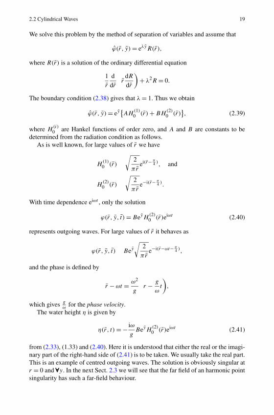
With time dependence eiωt , only the solution
ϕ(r, y, t ) = BeyH(2)0 (r)eiωt (2.40)
represents outgoing waves. For large values of r it behaves as
ϕ(r, y, t) ≈ Bey
√2
πre−i(r−ωt− π
4 ),
and the phase is defined by
r − ωt = ω2
g
(r − g
ωt
),
which gives gω
for the phase velocity.The water height η is given by
η(r, t) = − iω
gBeyH
(2)0 (r)eiωt (2.41)
from (2.33), (1.33) and (2.40). Here it is understood that either the real or the imagi-nary part of the right-hand side of (2.41) is to be taken. We usually take the real part.This is an example of centred outgoing waves. The solution is obviously singular atr = 0 and ∀∀∀y. In the next Sect. 2.3 we will see that the far field of an harmonic pointsingularity has such a far-field behaviour.

20 2 Linear Wave Phenomena
2.3 Harmonic Source Singularity
It is of interest to determine the field disturbance of the free surface due to an har-monic singularity in a point below or at the free surface. As will be shown in Chap. 3,many methods to solve the problem of diffraction of waves by an object we makeuse of a distribution of singularities at the surface of the object. Here we will de-termine the field generated by such a singularity. As an example we treat the finitewater depth case. The singularity is written as a Dirac δ-function in the right-handside of the Laplace equation
ϕxx + ϕyy + ϕzz = δ(x − x0, y − y0, z − z0)eiωt . (2.42)
If we introduce ϕ(x, y, z, t) = ϕ(x, y, z)eiωt , the boundary value problem to besolved becomes
ϕxx + ϕyy + ϕzz = δ(x − x0, y − y0, z − z0),
ϕy = 0 at y = −h,
ϕy = ω2
gϕ at y = 0.
(2.43)
This formulation is not complete. We must add a condition at large horizontal dis-tance from the source. The solution must fulfil the radiation condition. The distur-bance for large values of R = √
(x − x0)2 + (z − z0)2 may only consist of outgoingwaves. The solution must have the form
ϕ(x, y, z, t) ≈ A(R,y)e−i(kR−ωt), (2.44)
where the amplitude function tends to zero if R → 0.There are several ways to solve this problem. We shall employ the method of
Fourier transform to obtain a solution. We introduce the following exponential trans-form of ϕ with respect to the x and z coordinates
φ(α,y,β) =∫ ∞
−∞
∫ ∞
−∞ei(αx+βz)ϕ(x, y, z)dx dz. (2.45)
The inverse transform is
ϕ(x, y, z) = 1
4π2
∫ ∞
−∞
∫ ∞
−∞e−i(αx+βz)φ(α, y,β)dα dβ. (2.46)
We introduce the transform in the Laplace equation and the boundary conditionsfor ϕ and obtain an ordinary differential equation for φ with appropriate boundaryconditions
φyy − (α2 + β2)φ = ei(αx0+βz0)δ(y − y0),
φy = 0 at y = −h,
φy = ω2
gφ at y = 0.
(2.47)

2.3 Harmonic Source Singularity 21
The singularity in the right-hand side of the differential equation can be replaced bythe following conditions for the function φ(α,β, y):
limε→0
(φy(α, y0 + ε,β) − φy(α, y0 − ε,β)) = ei(αx0+βz0),
limε→0
(φ(α, y0 + ε,β) − φ(α,y0 − ε,β)) = 0.(2.48)
The solution of the problem is written as φ+ for y0 < y ≤ 0 and φ− for−h < y < y0. A convenient choice of the solution is
φ+ = A cosh(k(y + h)) + B sinh(k(y + h)),
φ− = C cosh(k(y + h)).
Here k is defined as the distance to the origin in the Fourier space which is thepositive root of k2 = α2 + β2. With this choice the bottom condition is fulfilledautomatically. The constants A,B and C are determined by the condition at the freesurface y = 0 together with the conditions at y = y0. After some manipulations wefind the solution for y0 < y ≤ 0,
φ+ = −cosh(k(y0 + h)){ν sinh(ky) + k cosh(ky)}k{k sinh(kh) − ν cosh(kh)} ei(αx0+βz0), (2.49)
and for −h < y < y0,
φ− = −cosh(k(y + h)){ν sinh(ky0) + k cosh(ky0)}k{k sinh(kh) − ν cosh(kh)} ei(αx0+βz0), (2.50)
where ν = ω2
g. We now apply the inverse transform given by (2.46) to φ+
ϕ+(x, y, z) = −1
4π2
∫ ∞
−∞
∫ ∞
−∞e−i(α(x−x0)+β(z−z0))
· cosh(k(y0 + h)){ν sinh(ky) + k cosh(ky)}k{k sinh(kh) − ν cosh(kh)} dα dβ. (2.51)
It is convenient to introduce polar coordinates, both in the physical space and theFourier space. We introduce
x − x0 = R cos θ, z − z0 = R sin θ (2.52)
and
α = k cosϑ, β = k sinϑ. (2.53)
The solution can then be written as
ϕ+(x, y, z) = −1
4π2
∫ 2π
0
∫ ∞
0e−ikR cos(ϑ−θ)
· cosh(k(y0 + h)){ν sinh(ky) + k cosh(ky)}k sinh(kh) − ν cosh(kh)
dϑ dk. (2.54)

22 2 Linear Wave Phenomena
The integration with respect to ϑ can be carried out by making use of the followingdefinition of the Bessel function J0:
J0(kR) = 1
2π
∫ 2π
0e−ikR cos(ϑ−θ) dϑ. (2.55)
Hence, if we follow the same procedure for ϕ−, we obtain
ϕ+(x, y, z) = −1
2π
∫ ∞
0
cosh(k(y0 + h)){ν sinh(ky) + k cosh(ky)}k sinh(kh) − ν cosh(kh)
J0(kR)dk,
ϕ−(x, y, z) = −1
2π
∫ ∞
0
cosh(k(y + h)){ν sinh(ky0) + k cosh(ky0)}k sinh(kh) − ν cosh(kh)
J0(kR)dk.
(2.56)
Until this point the radiation condition is not used. We will see that to define a properinverse transform it has to be used. The integrands of the functions ϕ+,− each havea singularity for a real value of the denominator. Hence, the integrals are not welldefined. The equation k sinh(kh) − ν cosh(kh) = 0 has one real root together withan infinite number of purely imaginary roots. From the theory of Fourier integral weknow that the contour of integration has to pass, in the complex k-plane, above orbelow the singularity. The choice is determined by the radiation condition. A way todetermine the correct choice is to introduce a small artificial damping in the fluid. Ifwe assume the far field to be of the form e−i(kR−ωt) we see that the only choice forvanishing waves is to introduce a complex wave number of the form k = k − ik. Thenegative imaginary part of the wave number may be generated by some artificial,non-physical, damping. This indicates that the singularity on the real axis must bepassed above. Representation (2.56) for ϕ consists of different forms depending onwhether y is larger or smaller than y0. This might be not practical. One may obtain asingle expression if we use some lemmas from the theory of complex functions. Weuse the following lemma for analytic functions f (z) and g(z), while the functionf (z) has simple zeros zi in the complex plane. If we define f (z) = z sinh(zh) −ν cosh(zh) and g(z) = cosh(zp){ν sinh(zq) + z cosh(zq) respectively, then for|z| → ∞ the function g(z)
f (z)→ 0 fast enough and we have
g(z)
f (z)= g(0)
f (0)+
∑i
g(zi)γi
(1
z − zi
+ 1
zi
)with γi = 1
fz(zi), (2.57)
which is an expansion of g(z)f (z)
in rational fractions of z, see [21], Sect. 7.4.The integrands of both integrals in the expression for ϕ(x, y, z) (2.56) has in-
finitely many simple poles k = ±ki (i = 0,1,2, . . .) in the complex k-plane. Wehave
ki sinh(kih) − ν cosh(kih) = 0. (2.58)
The positive real zero is k0, while the positive imaginary roots are ki = iκi (i =1,2, . . .), see Fig. 2.2.

2.3 Harmonic Source Singularity 23
Fig. 2.2 The singularities inthe complex k-plane
According to (2.57) we may write
g(k)
k sinh(kh) − ν cosh(kh)=
∞∑i=0
g(ki)
(α+
i
k − ki
+ α−i
k + ki
), (2.59)
where we used the fact that in our case g(k) is antisymmetric and g(0) = 0 andwhere αi is defined as
α±i = ±ki
(ν + k2i h − ν2h) cosh(kih)
. (2.60)
If we work out the integrands of (2.56) we find one expression for ϕ(x, y, z), validfor −h < y ≤ 0. We obtain
ϕ(x, y, z) = −1
2π
∞∑i=0
k2i − ν2
ν + k2i h − ν2h
cosh(ki(y + h)) cosh(ki(y0 + h))
·∫ ∞
0
(1
k − ki
− 1
k + ki
)J0(kR)dk. (2.61)
The integral in the right hand side can, by introducing k = −k∗ in the second part,be rewritten as
J (ki) = 1
2
∫ ∞
−∞H
(1)0 (kR)
k − ki
dk + 1
2
∫ ∞
−∞H
(2)0 (kR)
k − ki
dk. (2.62)
Due to the asymptotic behaviour of the Hankel functions we may close the firstintegral in the upper half of the complex k plane, while the second one may beclosed in the lower half. In this way the contributions of the contours at |k| → ∞tend to zero. If the path of integration in (2.62) passes the singularity k = k0 in theupper plane we obtain the following result for i = 0:
J (k0) = −π iH(2)0 (k0R), (2.63)

24 2 Linear Wave Phenomena
Fig. 2.3 Line of integration
and for i = 1,2, . . .
J (ki) = π iH(1)0 (iκiR) = 2K0(κiR), (2.64)
where K0(z) is the modified Bessel function. The contribution of H(2)0 (k0R) rep-
resents an outgoing circular wave, while the contribution of each K0(κiR) is expo-nential decaying for large values of R. This confirms the right choice of the contourof integration, see Fig. 2.3. We notice that the use of an artificial damping to shift k0actually is not the only way to find the correct contour of integration. If one choosesthe contour to pass underneath k0 the wavy behaviour is described by H
(1)0 (k0R),
describing an incoming circular wave field. Waves travelling towards the sourceclearly which disobey the radiation condition.
The expression for the total field now becomes
ϕ(x, y, z, t) = eiωt ϕ(x, y, z)
with
ϕ(x, y, z) = i(k20 − ν2)
2(ν + k20h − ν2h)
cosh(k0(y + h)) cosh(k0(y0 + h))H(2)0 (k0R)
+ 1
π
∞∑i=1
κ2i + ν2
ν − κ2i h − ν2h
cos(κi(y + h)) cos(κi(y0 + h))
× K0(κiR). (2.65)
If we take the real part of (2.65) and multiply it with −4π we have the famous resultof F. John. The different factor originates from the normalisation of the point source.This formulation can be used to compute the disturbance due to a unit point sourceat finite difference from the source. However, the series does not converge close tothe source. This was to be expected, because of the singular, −1
4πr, behaviour of ϕ,
where r = √(x − x0)2 + (y − y0)2 + z − z0)2 is the distance to the singularity.
We expect to find a useful solution near the singularity if we write it as
ϕ(x, y, z) = − 1
4πr− 1
4πr+ ψ(x, y, z), (2.66)
where r = √(x − x0)2 + (y + 2h + y0)2 + (z − zo)2 is the distance to the mirror
image, with respect to the bottom, of the source point. For ψ(x, y, z) we obtain the

2.3 Harmonic Source Singularity 25
following problem:
ψxx + ψyy + ψzz = 0,
ψy = 0 at y = −h,
ψy − νψ = 1
4π
{∂
∂y
(1
r+ 1
r
)− ν
(1
r+ 1
r
)}
:= g(x, z;x0, y0, z0)
at y = 0.
(2.67)
We apply the double Fourier transform to the function ψ ,
�(α,y,β) =∫ ∞
−∞
∫ ∞
−∞ei(αx+βz)ψ(x, y, z)dx dz (2.68)
and introduce polar coordinates (2.56) in the Fourier space. The ordinary differentialequation and boundary conditions for � become
�yy − k2� = 0,
�y = 0 at y = −h,
�y − ν� = G(k;x0, y0, z0) at y = 0.
(2.69)
We make use of the known transform of −14πr
, the point source for an infinite fluidwhere no free surface is present
F
( −1
4πr
)= −1
2kei(αx0+βz0)−k|y−y0|. (2.70)
This formula can be obtained by means of the double Fourier transform to theLaplace equation, as before, in the case of an infinite fluid. If we apply this for-mula to g(x, z;x0, y0, z0) we obtain
G(k;x0, y0, z0) = −k + ν
ke−kh cosh(k(y0 + h))ei(αx0+βz0) (2.71)
and the solution of (2.69) becomes
�(α,y,β) = −k + ν
ke−kh cosh(k(y + h)) cosh(k(y0 + h))
k sinh(kh) − ν cosh(kh)ei(αx0+βz0). (2.72)
The inverse Fourier transform is defined as
ψ(x, y, z) = 1
4π2
∫ ∞
−∞
∫ ∞
−∞�(α,y,β)e−i(αx+βz) dα dβ. (2.73)
With the introduction of polar coordinates in the physical (2.52) and Fourier (2.53)space we obtain with the use of (2.55) the total field
ϕ(x, y, z, t) = eiωt ϕ(x, y, z)

26 2 Linear Wave Phenomena
with
ϕ(x, y, z) = − 1
4πr− 1
4πr
− 1
2π
∫ ∞
0
(k + ν)e−kh cosh(k(y + h)) cosh(k(y0 + h))
k sinh(kh) − ν cosh(kh)J0(kR)dk.
(2.74)
If we introduce some artificial damping in the problem we observe that the contourof integration passes above the real pole in the integrand. This finally leads to theexpression
ϕ(x, y, z)
= − 1
4πr− 1
4πr
− 1
2π−∫ ∞
0
(k + ν)e−kh cosh(k(y + h)) cosh(k(y0 + h))
k sinh(kh) − ν cosh(kh)J0(kR)dk
+ i
2
(k0 + ν)e−k0h sinh(k0h) cosh(k0(y + h)) cosh(k0(y0 + h))
νh + sinh2(k0h)J0(k0R),
(2.75)
where −∫ indicates the principal value of the integral. If we are interested in the deepwater case we may obtain an expression for the source potential by using (2.75) forlarge values of h. We obtain for the limit h → ∞,
ϕ(x, y, z) = − 1
4πr− 1
4π−∫ ∞
0
k + ν
k − νek(y+y0)J0(kR)dk + i
2νeν(y+y0)J0(νR).
(2.76)This result may be rewritten as
ϕ(x, y, z) = − 1
4πr+ 1
4πr− 1
4π−∫ ∞
0
2k
k − νek(y+y0)J0(kR)dk+ i
2νeν(y+y0)J0(νR),
(2.77)where r = √
(x − x0)2 + (y + y0)2 + (z − z0)2 is the distance to the mirror point,with respect to the unperturbed free surface.
The contour of integration may be deformed to obtain different forms of (2.74).We can rewrite the integral as a contribution of the pole and an integral along thevertical axis of the complex k-plane. Instead of the way the solution is written in(2.76) one also may write the solution as the sum −( 1
4πr+ 1
4πr), where − 1
4πris the
field of a singularity located at (x0,−y0, z0) in an infinite fluid, and use an integralexpression for this term. There are more choices possible, they are sometimes usedin the literature for different reasons.

2.4 The Moving Pressure Point 27
2.4 The Moving Pressure Point
We consider the field generated by a pressure point disturbance at the free surface,moving in the direction of the positive x-axis. For small amplitude waves the lin-earised free surface condition is defined by (1.32). We suppose the bottom at infinity,y = −∞. Hence the bottom condition is replaced by the condition that ϕ remainsfinite as y → −∞. We look for a very simple solution in a steady flow, for whicheverywhere at y = 0 except at x = z = 0 the pressure vanishes. By introducing thedimensionless coordinates
x = xg
U2, y = yg
U2, z = zg
U2,
we can formulate the boundary value problem as follows;
ϕxx + ϕyy + ϕzz = 0,
ϕxx + ϕy = 0 at y = 0, (x, z) �= (0,0),
ϕ finite as y → ∞.
(2.78)
We seek solutions of (2.78) by means of a Fourier transform with respect to x,
ϕ(α, y, z) =∫ ∞
−∞eiαxϕ(x, y, z)dx (2.79)
with its inverse transform
ϕ(x, y, z) = 1
2π
∫ ∞
−∞e−iαx ϕ(α, y, z)dα. (2.80)
This leads to the boundary value problem for ϕ(α, y, z):
ϕyy + ϕzz − α2ϕ = 0,
−α2ϕ + ϕy = 0 at y = 0,
ϕ finite as y → −∞.
(2.81)
A simple solution of (2.81) can be found in the form
ϕ = eα2yF (z),
where F(z) satisfies the equation
(α4 − α2)F + Fzz = 0.
Consequently, we take as a possible solution
ϕ(x, y, z) = A
2π
∫ ∞
−∞exp
{−iαx + α2y + iα(α2 − 1)12 z
}dα, (2.82)

28 2 Linear Wave Phenomena
for A being a constant. Note that ϕ(x, y, z) is not defined for x = y = z = 0. From(1.33) we find the free surface elevation
η(x, z) = Ai
2πUlimy→0
∫ ∞
−∞(αeα2y
)exp
{i(−αx + α(α2 − 1)
12 z
)}dα (2.83)
which apparently is infinite for x = z = 0.In order to get a better insight into the shape of the surface we shall evaluate this
expression (2.83) for large values of x and z; that is distances to the origin that arelarge compared to the reference length U2/g. This evaluation is performed by themethod of stationary phase (see Sect. 9.1).
We note that if we let R = (x2 + z2)12 , x = R cosϑ and z = R sinϑ , then for each
fixed ϑ , (2.83) can be written in the form
∫ ∞
−∞g(α) exp(iRf (α))dα,
where
g(α) := Ai
2πUα and
Rf (α) := −αx + α(α2 − 1)12 z.
Hence the stationary points are solutions of the equation
∂
∂α
{−αx + α(α2 − 1)12 z
} = 0. (2.84)
(cf. (9.13)).Let α0 be a solution of (2.84). We obtain therefore the asymptotic form of η(x, z):
η(x, z) ∼= Ai
πUα0
√√√√π iα0(α20 − 1)
32
2z(2α20 − 3)
exp{i(−α0x + α0(α
20 − 1)
12 z
)}(2.85)
The phase function is of the most importance. If we put
ψ = −α0x + α0(α20 − 1)
12 z, (2.86)
we obtain from (2.84)
−x + 2α20 − 1√
α20 − 1
z = 0. (2.87)
2.5 Wave Fronts 29
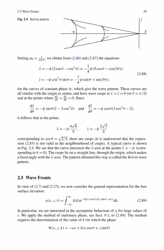
Fig. 2.4 Kelvin pattern
Setting α0 = 1cos θ
, we obtain from (2.86) and (2.87) the equations
x = −ψ(2 cos θ − cos3 θ) = −1
4ψ(5 cos θ − cos(3θ)),
z = −ψ cos2 θ sin θ = −1
4ψ(sin θ + sin(3θ))
(2.88)
for the curves of constant phase ψ , which give the wave pattern. These curves areall similar with the origin as centre, and have wave cusps at x = z = 0 (or θ = π/2)and at the points where dx
dθ= dz
dθ= 0. Since
dx
dθ= −ψ sin θ(2 − 3 cos2 θ) and
dz
dθ= −ψ cos θ(3 cos2 θ − 2),
it follows that at the points
x = −ψ4√
6
9, z = −ψ
2√
3
9
corresponding to cos θ = √2/3, there are cusps (it is understood that the expres-
sion (2.85) is not valid in the neighbourhood of cusps). A typical curve is shownin Fig. 2.4. We see that the curve intersects the x-axis at the points x = −ψ (corre-sponding to θ = 0). The cusps lie on a straight line, through the origin, which makesa fixed angle with the x-axis. The pattern obtained this way is called the Kelvin wavepattern.
2.5 Wave Fronts
In view of (2.7) and (2.23), we now consider the general representation for the freesurface elevation:
η(x, z, t) =∫ ∞
−∞A(k)e−i(kx cos θ+kz sin θ−ωt) dk. (2.89)
In particular, we are interested in the asymptotic behaviour of η for large values oft . We apply the method of stationary phase, see Sect. 9.1, to (2.89). The methodrequires the determination of the value of k for which the phase
�(x, z, k) = −ωt + k(x cos θ + z sin θ)

30 2 Linear Wave Phenomena
= −t
[k
(x
tcos θ + z
t
)− ω(k)
](2.90)
is stationary. (Here we consider � as depending on the three parameters xt, z
tand t .
For each pair of values of xt
and zt, the asymptotic expansion for η is considered for
large t .) This leads to the consideration of solutions of the equations
d�
dk= 0 or − dω
dkt + x cos θ + z sin θ = 0. (2.91)
Let k0 be any solution of (2.91). Then the approximate result for large t is
η(x, z, t) = A(k0)
√2π
t |ω′′(k0)|e−i(k0x cos θ+k0z sin θ−ω(k0)t− π4 sgnω′′(k0)) (2.92)
provided that d2�(k0)
dk2 �= 0, i.e. ω′′(k0) �= 0.The lines � = constant are lines of constant phase; these lines are called wave
fronts. We can define a partial differential equation for the wave fronts from thedispersion relation ω = H(k). In fact, we can express k0 in terms of x, z, t and θ
from (2.92) so that differentiations of (2.91) (with k = k0) with respect to thesevariables yield
�x = k0 cos θ + (x cos θ + z sin θ − ω′0t)
∂k0
∂x= k0 cos θ,
�z = k0 sin θ + (x cos θ + z sin θ − ω′0t)
∂k0
∂z= k0 sin θ,
�t = −ω0 + (x cos θ + z sin θ − ω′0t)
∂k0
∂t= −ω0,
(2.93)
with ω0 = H(k0). The first two equations of (2.93) imply that
k20 = �2
x + �2z
with which the third one shows that the dispersion relation ω0 = H(k0) gives apartial differential equation for the phase function � , the Hamilton-Jacobi equation
�t + H(
√�2
x + �2y ) = 0 or
�t + H(
√p2 + q2) = 0,
(2.94)
where p = �x = k0 cos θ and q = �z = k0 sin θ are the conjugate variables to x
and z, respectively. We have just seen that the wave fronts correspond to level curvesof the Hamilton-Jacobi equation. But in wave phenomena one expects the dual con-cept of rays to appear also. The rays in the present case are the characteristics of the

2.6 Wave Patterns 31
Fig. 2.5 Wave fronts
above Hamilton-Jacobi equation, i.e. the solutions of the system of ODE’s:
dx
dt= ∂H
∂p,
dp
dt= −∂H
∂x= 0,
dz
dt= ∂H
∂q,
dq
dt= −∂H
∂z= 0
(2.95)
(see Sect. 9.2 for a brief summary of the concepts of characteristics). From the(2.95) it is easy to see that in the x, z, t-space, the characteristics are straight linesfor constant t as in (2.91).
2.6 Wave Patterns
In Sect. 2.5, the Hamilton-Jacobi equation (2.94) for the wave fronts was derivedfrom the equations in a rather complicated way. At first we gave an exact solutionη of the linearised problem (1.32), (1.33) with U = 0, to which we later applied anasymptotic expansion, which resulted in a first-order partial differential equation.The result obtained is more or less similar to the characteristic equation for hyper-bolic equations, although the wave fronts are by no means characteristic surfacesfor the equations, which do not even have real characteristics.
In order to give a direct derivation we first define a wave front on the two-dimensional x, y-plane as a curve along which a transverse derivative of the so-lution ϕ of the equation considered is much larger than the tangential derivative.This means that, introducing new coordinates ξ1 transverse to the wave fronts andξ2 along the wave fronts (Fig. 2.5), we must have that ϕξ1 ϕξ2 , i.e. there shouldexist a constant K 1 such that ϕξ1 ≈ Kϕξ2 . Here ξ1 and ξ2 are supposed to befunctions of x and y with derivatives of order unity with respect to K . We introducea new coordinate s = Kξ1 such that
ϕs = 1
Kϕξ1 = O(1). (2.96)
We now illustrate this procedure by considering a simpler equation than the equationof water waves, the Klein-Gordon equation in dimensionless form
ϕxx − ϕtt − a2ϕ = 0, (2.97)
32 2 Linear Wave Phenomena
where a is a constant. We first derive the Hamilton-Jacobi equations for the phasefunction to the methods used in Sect. 2.5 and will refer to it as an indirect method.For solutions of the form Aei(kx−ωt) we easily find the dispersion relation betweenk and ω,
ω =√
a2 + k2 � H(k) (2.98)
which gives the Hamilton-Jacobi equation from (2.94) with � = J :
Jt + H(Jx) = 0, (2.99)
where Jx = k. The characteristics of (2.99) are solutions of the equations
dx
dt= ∂H
∂Jx
= k√a2 + k2
,
dp
dt= dJx
dt= −∂H
∂x= 0,
(2.100)
thus the characteristics are straight lines of the form
x − k√a2 + k2
t = constant, (2.101)
corresponding to the group velocity dHdk
= k√a2+k2
.
Now let us examine the above problem by the direct method. Using (2.96),a straightforward calculation shows that
ϕxx = K2ϕssξ21x + K(2ϕsξ2ξ1xξ2x + ξ1xxϕs) + ϕξ2ξ2ξ
22x + ϕξ2ξ2xx,
ϕtt = K2ϕssξ21t + K(2ϕsξ2ξ1t ξ2t + ξ1t t ϕs) + ϕξ2ξ2ξ
22t + ϕξ2ξ2t t .
(2.102)
Substituting into (2.97) gives
K2ϕss(ξ21x − ξ2
1t ) + K{ϕs(ξ1xx − ξ1t t ) + 2ϕsξ2(ξ1xξ2x − ξ1t ξ2t )}+ ϕξ2ξ2(ξ
22x − ξ2
2t ) + ϕξ2(ξ2t − ξ2t t ) − a2ϕ = 0. (2.103)
As K → ∞, we obtain the characteristic equation for (2.97). This is obvious be-cause a characteristic would be a line along which the second derivative may bediscontinuous. Now, regarding the constant a as a large number with respect tosome reference length and identifying K with a, we have the equation
ϕss(ξ21x − ξ2
1t ) − ϕ = 0, (2.104)
to the first order of approximation. If we want this equation to represent the motionalong the wave fronts, we must put the term (ξ2
1x − ξ21t ) equal to a constant which
we choose to be −1, i.e.,
ξ21x − ξ2
1t = −1. (2.105)

2.6 Wave Patterns 33
Clearly, this gives immediately the Hamilton-Jacobi equation, ξ1t =√
1 + ξ21x ,
which reduces to (2.99) with ξ1 replaced by (−1/a)J .The same scheme can be applied to the problem of the moving singularity defined
by the time independent form (1.32) and (1.33), i.e.:
ϕxx + ϕyy + ϕzz = 0,
U2ϕxx + gϕy = 0, for y = 0.
In terms of the dimensionless variables x = xL, y = y
Land z = z
L, we have
ϕxx + ϕyy + ϕzz = 0,
ϕxx + gL
U2ϕy = 0, for y = 0.
(2.106)
Here L denotes a proper reference length.We are only interested in the wave pattern, hence in the lines of constant phase
of η (which from (1.33) amounts to the same as for ϕx at y = 0). We further remarkthat from the nature of (2.106) we know that the wave is only appreciable at theupper layer of the water. Hence we introduce the coordinates ξ1 and ξ2 in the x, z-plane, where the lines ξ1 = constant represent wave fronts, the derivative ϕξ1 is largewith respect to ϕξ2 but the derivative ϕy must be of the same order of magnitude asϕξ1 . Therefore, we introduce a coordinate s = Kξ1 and a coordinate Y = Ky interms of which we have
ϕxx = K2ϕssξ21x + K(2ϕsξ2ξ1xξ2x + ξ1xxϕs) + ϕξ2ξ2ξ
22x + ϕξ2ξ2xx,
ϕzz = K2ϕssξ21z + K(2ϕsξ2ξ1zξ2z + ξ1zzϕs) + ϕξ2ξ2ξ
22z + ϕξ2ξ2zz,
and
ϕyy = K2ϕYY .
From (2.106), we have then
K2ϕss(ξ21x + ξ2
1z) + K2ϕYY + O(K) = 0, (2.107)
together with the surface condition
K2ϕssξ21x + K
(gL
U2
)ϕY + O(K) = 0, for Y = 0. (2.108)
This yields the first approximation
ϕss(ξ21x + ξ2
1z) + ϕYY = 0,
ϕssξ21x + ϕY = 0, for Y = 0,
(2.109)
where we identify K with gL
U2 .

34 2 Linear Wave Phenomena
Since ξ21x + ξ2
1z and ξ21x are slowly varying variables, we introduce constants,
α and β defined by
α2 = ξ21x + ξ2
1z, and β = ξ21x.
This leads to the problem
α2ϕss + ϕYY = 0,
βϕss + ϕY = 0, for Y = 0,
which has a solution
ϕ = eis+.αY .
This solution which goes to zero as Y → ∞ (α > 0) can satisfy the surface conditiononly if
α = β
or
ξ21x + ξ2
1z = ξ41x. (2.110)
It should be emphasised that these considerations are only valid to an order of mag-nitude of 1/K . The present approach is a variation of the ray method in geometricaloptics. Higher-order approximations can be derived in a similar manner.
The characteristic equations of the first-order partial differential equation (2.110)take the form
x = 4p3 − 2p, p = 0,
z = −2q, q = 0,
ξ1 = (4p4 − 2p2 − 2q2),
with p = ξ1x and q = ξ1z, where the dot · notation denotes differentiation to someparameter, say, τ . Hence p and q are constants and we have the parametric equationsfor the rays,
x = 2p(2p2 − 1)τ,
z = −2qτ,
ξ1 = (4p4 − 2p2 − 2q2)τ.
(2.111)
From (2.110) we have
q = −p
√p2 − 1. (2.112)
To eliminate τ from (2.111) by making use of (2.112), we finally obtain
x = ξ1(2p2 − 1)
p3, z = ξ1
√p2 − 1
p3,

2.7 Singularity in a Steady Current 35
which reduces to (2.88) if we set p = − 1cos θ
. This shows that the curves ξ1 = con-stant are indeed the curves of constant phase.
2.7 Singularity in a Steady Current
2.7.1 Steady Singularity
As in the case of an oscillatory point source in still water it is useful to have thesolution of a steady moving point source, or a point source in a steady current,available. For finite water depth the formulation becomes
ϕxx + ϕyy + ϕzz = δ(x − x0, y − y0, z − z0),
ϕy = 0 at y = −h,
υϕxx + ϕy = 0 at y = 0,
(2.113)
where we introduced the notation υ = U2
g. To obtain a physically valid solution
we have to add a far-field condition, comparable with the radiation condition inthe oscillatory case. Here the requirement becomes that in front of the disturbanceno wavy pattern is observed. In the downstream region a wavy disturbance may bepresent. In the deep water case it is similar to the disturbance of the moving pressurepoint. It is also noticed that a solution of (2.113) can not be unique, because wealways may add an arbitrary constant. We make use of this fact later. We follow thesame procedure as described before (2.66) to solve (2.113),
ϕ(x, y, z) = − 1
4πr− 1
4πr+ ψ(x, y, z), (2.114)
where r denotes the distance to reflected, with respect to the bottom, source point.For ψ(x, y, z) we obtain the formulation
ψxx + ψyy + ψzz = 0,
ψy = 0 at y = −h,
ψy + υψxx = 1
4π
{∂
∂y
(1
r+ 1
r
)+ υ
∂2
∂x2
(1
r+ 1
r
)}
:= r(x, z;x0, y0, z0)
at y = 0.
(2.115)
If we apply the double Fourier transform to the function ψ ,
�(α,y,β) =∫ ∞
−∞
∫ ∞
−∞ei(αx+βz)ψ(x, y, z)dx dz, (2.116)

36 2 Linear Wave Phenomena
we obtain the following ordinary differential equation and boundary conditionsfor �:
�yy − (α2 + β2)� = 0,
�y = 0 at y = −h,
�y − υα2� = R(α,β;x0, y0, z0) at y = 0.
(2.117)
Application of (2.70) leads to the following expression for R(α,β;x0, y0, z0),
R(α,β;x0, y0, z0) = −k + υα2
ke−kh cosh(k(y0 + h))ei(αx0+βz0), (2.118)
where k = √α2 + β2. The solution of (2.117) becomes
�(α,y,β) = −k + υα2
ke−kh cosh(k(y + h)) cosh(k(y0 + h))
k sinh(kh) − υα2 cosh(kh)ei(αx0+βz0). (2.119)
The inverse transform (2.73) of �(α,y,β) becomes
ψ(x, y, z) = −1
4π2
∫ ∞
−∞
∫ ∞
−∞e−kh cosh(k(y + h)) cosh(k(y0 + h))
· k + υα2
k
e−i(α(x−x0)+β(z−z0))
k sinh(kh) − υα2 cosh(kh)dα dβ (2.120)
and after the introduction of polar coordinates in the Fourier plane (2.52), (2.53)
ψ(x, y, z) = −1
4π2
∫ ∞
0
∫ 2π
0e−kh cosh(k(y + h)) cosh(k(y0 + h))
· (1 + kυ cos2 ϑ)e−ik((x−x0) cosϑ+(z−z0) sinϑ)
sinh(kh) − kυ cos2 ϑ cosh(kh)dk dϑ. (2.121)
The integral is singular at k = 0. Therefor we make use of the fact that we may adda constant, with respect to x, y and z to the solution of (2.113). Hence a solution of(2.113) may be written as
ϕ(x, y, z) = − 1
4πr− 1
4πr+ ψ(x, y, z) (2.122)
with
ψ(x, y, z) = −1
4π2
∫ ∞
0dk
∫ 2π
0dϑ
e−kh
sinh(kh) − kυ cos2 ϑ cosh(kh)
· {cosh(k(y + h)) cosh(k(y0 + h))(1 + kυ cos2 ϑ)
· e−ik((x−x0) cosϑ+(z−z0) sinϑ) − 1}. (2.123)

2.7 Singularity in a Steady Current 37
This solution does not fulfil the condition that upstream (x → −∞) no wavy dis-turbance may be present. To obey this condition a path of integration along thesingularity on the real k-axis has to be chosen. Depending on the sign of cosϑ thechoice will be different.
We notice that for cosϑ > 0 and x − x0 > 0 we may close the integral withrespect to k in the fourth quadrant of the complex k-plane. For cos2 ϑ < h
υwe find
a simple pole on the real k-axis. This means that to obtain a wavy contribution thissingularity on the real axis must be inside the contour. We obtain a contribution ofthe pole plus an integral along the negative imaginary axis. This integral representsan exponentially decaying contribution. If however x − x0 < 0 we close the integralin the first quadrant and we obtain a contribution of an integral along the positiveimaginary axis only.
Next we consider cosϑ < 0 and x − x0 > 0 and we may close the integral in thefirst quadrant of the complex k-plane. We obtain a contribution of the singularity onthe real axis if we chose the pole inside the contour. Again the integral along theimaginary axis is exponentially decaying. If x − x0 < 0 we may close the contourin the fourth quadrant. This gives rise to a decaying contribution only.
We may reformulate the integral part of the solution by splitting up the integrationwith respect to ϑ into four parts of length π/2 and to combine the integral. In thisway we obtain
ψ(x, y, z) = − 1
π2
∫ ∞
0dk
∫ π2
0dϑ
e−kh
sinh(kh) − kυ cos2 ϑ cosh(kh)
{cosh(k(y + h))
· cosh(k(y0 + h))(1 + kυ cos2 ϑ) cos((x − x0)
· cosϑ) cos((z − z0) sinϑ) − 1}. (2.124)
In the Handbook of Physics [19], Wehausen gives further details of this expression.To obtain an expression for the deep water case we let h → ∞ in expression
(2.123) and obtain.
ϕ(x, y, z) = − 1
4πr+ 1
4πr− 1
2π2
∫ ∞
0dk
∫ π
0dϑ
1
1 − kυ cos2 ϑ
· ek((y+y0)−i(x−x0) cosϑ) cos(k(z − z0) sinϑ) (2.125)
where we used (2.70) to obtain the contribution of a singularity at the point(x0,−y0, z0), hence r is defined as
√(x − x0)2 + (y + y0)2 + (z − z0)2. The con-
tour in the k-plane has to be chosen as before. For cosϑ > 0 the contour passes thesingularity in the upper plane, while for cosϑ < 0 the contour passes the singularityin the lower plane. The contribution of the pole gives a far-field pattern comparablewith the moving pressure point wave field described in Sect. 2.4.

38 2 Linear Wave Phenomena
2.7.2 Oscillating Singularity
The boundary value problem for the disturbance of a steady flow is describedin (1.32). We consider a harmonic point source and assume that the potential func-tion can be written as
φ(x, y, z, t) = eiωt φ(x, y, z).
The boundary value problem for the disturbance of a point source in (x0, y0, z0)becomes
ϕxx + ϕyy + ϕzz = δ(x − x0, y − y0, z − z0)eiωt . (2.126)
If we introduce ϕ(x, y, z, t) = ϕ(x, y, z)eiωt , the boundary value problem to besolved becomes
ϕxx + ϕyy + ϕzz = δ(x − x0, y − y0, z − z0),
ϕy = 0 at y = −h,
υφxx + 2iτ ϕx − νϕ + ϕy = 0 at y = 0,
(2.127)
where we introduced the parameters ν = ω2/g, υ = U2/g,and τ = (ωU)/g; noticethat τ 2 = νυ .
ϕ(x, y, z) = − 1
4πr− 1
4πr+ ψ(x, y, z). (2.128)
Introduction of the double Fourier transform leads to the following ordinary differ-ential equation for the transform of ψ ,
�yy − (α2 + β2)� = 0,
�y = 0 at y = −h,
�y − (υα2 + 2τα + ν)� = S(α,β;x0, y0, z0) at y = 0.
(2.129)
Application of (2.70) leads to the following expression for S(α,β;x0, y0, z0),
S(α,β;x0, y0, z0) = −k + υα2 + 2τα + ν
ke−kh cosh(k(y0 + h))ei(αx0+βz0),
(2.130)where k = √
α2 + β2. The solution of (2.129) becomes
�(α,y,β) = −k + υα2 + 2τα + ν
ke−kh
· cosh(k(y + h)) cosh(k(y0 + h))
k sinh(kh) − (υα2 + 2τα + ν) cosh(kh)ei(αx0+βz0). (2.131)
The inverse transform of �(α,y,β) gives the solution of (2.127). The choice of thepath of integration will be elucidated in the deep water case. Hence we consider the
2.7 Singularity in a Steady Current 39
limit h → ∞. We rewrite expression (2.131) in the form
�(α,y,β) =(
1
2− L (k,α)
)ek(y+y0)ei(αx0+βz0)
k. (2.132)
The function L (k,α) becomes, in polar coordinates in the Fourier plane,
limh→∞L (k, θ) = k
k − (υα2 + 2τα + ν)= gk
gk − (ω + kU cos θ)2. (2.133)
Finally we obtain an expression for ϕ(x, y, z) where we still have to choose theproper path of integration in the complex k-plane
ϕ(x, y, z) = − 1
4πr+ 1
4πr− 1
2π2
∫ ∞
0
∫ π
0
gk
gk − (ω + kU cos θ)2
· ek((y+y0)−i(x−x0) cosϑ) cos(k(z − z0) sinϑ)dk dϑ. (2.134)
We will investigate the zeros of the denominator. The quadratic equation has twozeros,
gk± = 1 − 2τ cosϑ ± √1 − 4τ cosϑ
2τ 2 cos2 ϑω2. (2.135)
First of all we notice that, for values of ϑ for which we have
1 − 4τ cosϑ < 0, (2.136)
we find no singularities of the integrand along the real k-axis. Hence for τ > 1/4 wefind a ϑ interval where the k-integral is regular for 0 ≤ ϑ < γ with cosγ = 1/(4τ).For τ < 1/4 we have γ = 0. Next, to determine the contour of integration when twopoles lie on the positive real axis we have to consider the condition in the far field.It is easy to show that for ϑ > γ both roots of the quadratic equation are situated onthe positive real axis of the complex k-plane. It is convenient to consider the polesfor small values of U and ω successively. In both cases τ becomes small, so weconsider the two poles for τ → 0. We find
limτ→0
k− = ω2
gand lim
τ→0k+ = g
U2 cos2 ϑ. (2.137)
In the oscillatory case without current we have seen that the contour passes the polein the first quadrant of the complex k-plane, for all values of ϑ . Actually we couldcarry out the ϑ integral in that case. Hence, we conclude that this is also the case forthe singularity in k−.
In the case of a steady source in a current we have seen that we have to con-sider the sign of cosϑ because in the downstream direction the far field shows awavy character. Hence for cosϑ > 0 the contour of integration passes k+ in the first
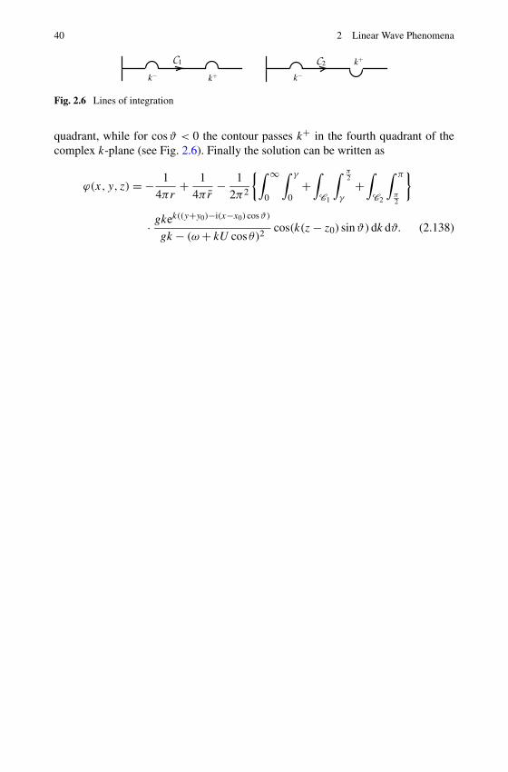
40 2 Linear Wave Phenomena
Fig. 2.6 Lines of integration
quadrant, while for cosϑ < 0 the contour passes k+ in the fourth quadrant of thecomplex k-plane (see Fig. 2.6). Finally the solution can be written as
ϕ(x, y, z) = − 1
4πr+ 1
4πr− 1
2π2
{∫ ∞
0
∫ γ
0+
∫C1
∫ π2
γ
+∫
C2
∫ π
π2
}
· gkek((y+y0)−i(x−x0) cosϑ)
gk − (ω + kU cos θ)2cos(k(z − z0) sinϑ)dk dϑ. (2.138)

Chapter 3Boundary Integral Formulation and ShipMotions
In the field of ship hydrodynamics the application of integral equations to solve thelinear ship motion problem is widely used. For linear problems harmonic in timethere are different ways to formulate an integral equation. A popular formulation,described in this chapter, is the one in the frequency domain. A less frequently usedapproach is a formulation in the time domain. The advantage of the latter approachis that the source function is rather simple and that it can be extended to the nonlinear case with some minor effort. For the steady ship wave problem a non-linearapproach is the currently most used. In this chapter we give an introduction to theseformulations. These methods consist of a description by means of regular Fredholmintegral equations. In this chapter we present the method based on Green’s theo-rem. To outline the method and the difficulties encountered we treat a simpler case,namely the diffraction of an acoustic wave by a smooth object. Hence we first con-sider the Helmholz equation for the scattering of acoustic waves, instead of the freesurface problem.
A short introduction is given to the linear ship motion problem. The structureof the equations of motion is explained by the treatment of an object that is freeto move in one degree of freedom, namely the vertical heave motion. The coeffi-cients equations of motion of the general problem, with six degrees of freedom,can be determined by means of the numerical solution of the integral equations forthe potential. In the same way the exciting forces may be computed. For the zeroforward speed case this approach is generally used. Extension to the forward speedcase is possible if the steady flow field around the ship does not differ much fromthe uniform velocity. Here we describe a way to apply a slow speed approximation.
3.1 Scattering of Acoustic Waves
The equation for a time dependent acoustic disturbance u(x, y, z, t) is the well-known wave equation
uxx + uyy + uzz = 1
c2ut t , (3.1)
A.J. Hermans, Water Waves and Ship Hydrodynamics,DOI 10.1007/978-94-007-0096-3_3, © Springer Science+Business Media B.V. 2011
41

42 3 Boundary Integral Formulation and Ship Motions
where c is the specific velocity of sound in the medium. We look for harmonic wavesolutions of this equation. Hence we look for solutions of the form
u(x, y, z, t) = u(x, y, z)eiωt . (3.2)
The function u now becomes a solution of the Helmholz equation
uxx + uyy + uzz + ω2
c2u = �u + k2u = 0 (3.3)
where � is the three-dimensional Laplace operator and k = ωc
is the wave number.The acoustic field due to a point source is a solution of
�u + k2u = δ(x − ξ, y − η, z − ζ ). (3.4)
The solution can be constructed by either introduction of spherical coordinates or inanalogy with the method used in Sect. 2.3 by means of a double Fourier transformperformed for instance in the x and z coordinates. We follow the former procedure.The solution of (3.4) only depends on the distance
r =√
(x − ξ)2 + (y − η)2 + (z − ζ )2 = |xxx − ξξξ |
to the source. We obtain the following ordinary differential equation for u(R),
urr + 2
rur + k2u = 0 for r �= 0. (3.5)
Hence the singular solution of (3.4) becomes a linear combination of u± = e±ik|xxx−ξξξ ||xxx−ξξξ | .
The solution of the source problem must consist of outgoing waves only, hence wechoose
u = − 1
4π
e−ik|xxx−ξξξ |
|xxx − ξξξ | . (3.6)
The choice of the factor − 14π
is easily checked by taking the limit case for k → 0.The result reduces to the singular solution of the Laplace equation where we requirea unit outgoing flux through a sphere around the source.
We shall construct some possible boundary integral formulation for the scatteringproblem. We consider a plane incident wave scattered by a smooth penetrable orimpenetrable convex object. The general boundary condition on the object is Au +B ∂u
∂n= 0, where n is along the normal at the scattering surface S , see Fig. 3.1.
In analogy with the ship wave problem we take as boundary condition ∂u∂n
= 0. Toobtain an integral equation along the surface we first consider a point (x, y, z) in thedomain D−, inside the object and apply Green’s theorem to the functions u and u.In the case of exterior scattering this is an artificial problem. We do so because itwill give us insight into the behaviour the mathematical formulation of the exterior
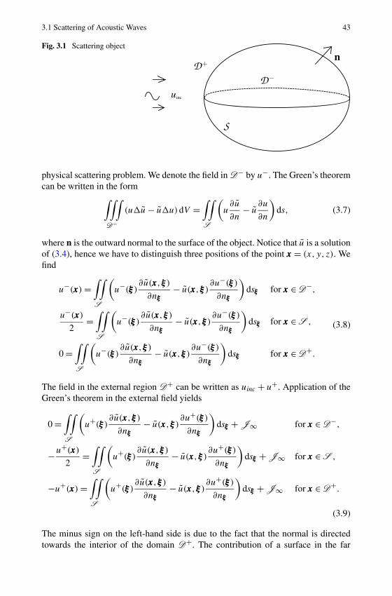
3.1 Scattering of Acoustic Waves 43
Fig. 3.1 Scattering object
physical scattering problem. We denote the field in D− by u−. The Green’s theoremcan be written in the form∫∫∫
D−(u�u − u�u)dV =
∫∫S
(u
∂u
∂n− u
∂u
∂n
)ds, (3.7)
where n is the outward normal to the surface of the object. Notice that u is a solutionof (3.4), hence we have to distinguish three positions of the point xxx = (x, y, z). Wefind
u−(xxx) =∫∫S
(u−(ξξξ)
∂u(xxx,ξξξ)
∂nξξξ
− u(xxx,ξξξ)∂u−(ξξξ)
∂nξξξ
)dsξξξ for xxx ∈ D−,
u−(xxx)
2=
∫∫S
(u−(ξξξ)
∂u(xxx,ξξξ)
∂nξξξ
− u(xxx,ξξξ)∂u−(ξξξ)
∂nξξξ
)dsξξξ for xxx ∈ S ,
0 =∫∫S
(u−(ξξξ)
∂u(xxx,ξξξ)
∂nξξξ
− u(xxx,ξξξ)∂u−(ξξξ)
∂nξξξ
)dsξξξ for xxx ∈ D+.
(3.8)
The field in the external region D+ can be written as uinc + u+. Application of theGreen’s theorem in the external field yields
0 =∫∫S
(u+(ξξξ)
∂u(xxx,ξξξ)
∂nξξξ
− u(xxx,ξξξ)∂u+(ξξξ)
∂nξξξ
)dsξξξ + J∞ for xxx ∈ D−,
−u+(xxx)
2=
∫∫S
(u+(ξξξ)
∂u(xxx,ξξξ)
∂nξξξ
− u(xxx,ξξξ)∂u+(ξξξ)
∂nξξξ
)dsξξξ + J∞ for xxx ∈ S ,
−u+(xxx) =∫∫S
(u+(ξξξ)
∂u(xxx,ξξξ)
∂nξξξ
− u(xxx,ξξξ)∂u+(ξξξ)
∂nξξξ
)dsξξξ + J∞ for xxx ∈ D+.
(3.9)
The minus sign on the left-hand side is due to the fact that the normal is directedtowards the interior of the domain D+. The contribution of a surface in the far
44 3 Boundary Integral Formulation and Ship Motions
field is denoted by J∞. We may take a sphere, S∞, with centre at (x0, y0, z0) andradius r . The far-field integral can then be written as
J∞ = −∫∫S∞
(u+ ∂u
∂r− u
∂u+
∂r
)ds
= limr→∞
1
4π
π2∫
− π2
2π∫0
(u+ ∂ e−ikr
r
∂r− e−ikr
r
∂u+
∂r
)r2 sin(θ)dθ dφ. (3.10)
The appropriate far-field conditions are
limr→∞u+ = 0 and lim
r→∞ r
(iku+ + ∂u+
∂r
)= 0. (3.11)
It is easy to show that r in this formulation can be taken as the distance to theorigin of the coordinate system. The latter condition is the well-known Sommerfeldradiation condition. Only outgoing waves are permitted in the scattered far field.We notice that if we had taken as time dependency e−iωt , the sign in the radiationcondition changes. So from now on we take J∞ = 0 in formulation (3.9).
There are several ways to obtain an integral equation for the exterior Neumannproblem. Hence the boundary condition for the function u+ becomes ∂u+
∂n= − ∂uinc
∂n
on S .
3.1.1 Direct Method
The second relation in (3.9) gives an integral equation for the function u+ on S .After solving this equation numerically, the function u+ in the domain D+ is thengiven by the third relation in (3.9). In a slightly different, commonly used, notationthe integral equation becomes
1
2u+(x) = −
∫∫S
(u+(ξξξ)
∂G(xxx,ξξξ)
∂nξξξ
+ G(xxx,ξξξ)∂uinc(ξξξ)
∂nξξξ
)dsξξξ
for xxx ∈ S , (3.12)
where
G(xxx,ξξξ) = u(xxx,ξξξ) = − 1
4π
e−ikr
r
with r = |xxx − ξξξ |.

3.1 Scattering of Acoustic Waves 45
3.1.2 Source Distribution
Let us combine (3.8) and (3.9). If we subtract the two expressions in the domainD+ we obtain the following expression for u+
−u+(xxx) =∫∫S
((u+(ξξξ) − u−(ξξξ))
∂G(xxx,ξξξ)
∂nξξξ
− G(xxx,ξξξ)∂(u+(ξξξ) − u−(ξξξ))
∂nξξξ
)dsξξξ .
(3.13)
The inner problem is an artificial one, so we may choose its boundary conditionon S . We take
u+(ξξξ) = u−(ξξξ) for ξξξ ∈ S
and define
σ(ξξξ) = ∂(u+(ξξξ) − u−(ξξξ))
∂nξξξ
for ξξξ ∈ S . (3.14)
The expression for u+ now becomes
u+(xxx) =∫∫S
σ(ξξξ)G(xxx,ξξξ)dsξξξ . (3.15)
This expression can be interpreted as a distribution of sources, over S , with strengthσ(ξξξ) and influence function G(xxx,ξξξ). For the Neumann problem we obtain an inte-gral equation by differentiating (3.15) with respect to the normal direction at thesurface. We obtain
∂u+(xxx)
∂nxxx
= −∂uinc(xxx)
∂nxxx
= 1
2σ(xxx) +
∫∫S
σ(ξξξ)∂G(xxx,ξξξ)
∂nxxx
dsξξξ . (3.16)
The question now arises whether this integral equation has a unique solution, whenthe exterior problem has a unique solution. The answer to this question is that forcertain frequencies the integral equation has a non-unique solution. This is easy toshow by studying the artificial interior formulation for a homogeneous Dirichletproblem, i.e., u− = 0 for xxx ∈ S . In this case we may formulate an integral equationfor the normal derivative u−
n at S . The first expression in (3.8) reads
u−(xxx) = −∫∫S
G(xxx,ξξξ)∂u−(ξξξ)
∂nξξξ
dsξξξ .
Differentiation of this expression in the direction of the normal yields
∂u−(xxx)
∂nxxx
= −∫∫S
∂G(xxx,ξξξ)
∂nxxx
∂u−(ξξξ)
∂nξξξ
dsξξξ for xxx ∈ D−.

46 3 Boundary Integral Formulation and Ship Motions
Fig. 3.2 Localapproximation
If we let xxx approach S from the inside region D− we have to evaluate the integralcarefully near the singular point. We consider the integral over the surface of asmall circle, with radius ρ, around the projection of the singular point, on S . Wemay consider the surface locally flat, see Fig. 3.2.
The integral may be approximated, for small values of the distance ε to the sur-face, by
1
4π
∂u−(xxx)
∂nxxx
ρ∫0
2π∫0
ε
(R2 + ε2)3/2R dR dθ = 1
2
∂u−(xxx)
∂nxxx
+ O(ε). (3.17)
Hence we obtain a relation for u−n at the surface:
1
2
∂u−(xxx)
∂nxxx
+∫∫S
∂G(xxx,ξξξ)
∂nxxx
∂u−(ξξξ)
∂nξξξ
dsξξξ = 0 for xxx ∈ S . (3.18)
The integral should be interpreted as the principle value integral over the surface S .It is well known that, at certain frequencies, the internal homogeneous Dirichletproblem exhibits resonance. Hence (3.18) has non-zero solutions at these frequen-cies. This means that the equation for the source function (3.16) has non-uniquesolutions at the same frequencies, while in the exterior region no resonance phe-nomenon occurs. The attempt to find a solution of the exterior Neumann problemby means of a source distribution breaks down at these irregular frequencies.
3.2 Scattering of Free Surface Waves
For offshore engineering one is interested in the forces and moments acting on fixedor floating structures. To compute these forces one must take into account the effectof the scattered field. Hence, we first consider the scattering of free surface wavesdue to a fixed floating object. The total wave field results in a pressure distribution

3.2 Scattering of Free Surface Waves 47
Fig. 3.3 Object in waves
along the object. Hence the forces and moments may be computed. If the body isfree to move in its six degrees of freedom it excites waves as well, resulting in theso-called reaction forces and moments. The forces and moments can be split up in apart in phase with the motion and a part out of phase with the motion. The first oneis generally associated with the so-called added mass and the second with the wavedamping.
3.2.1 Fixed Object
We first consider the scattering of waves at finite water depth by a fixed object, seeFig. 3.3. The potential in the outside domain D+ is written as
ϕ(x, y, z, t) = ϕ(x, y, z)eiωt = (φinc(x, y, z) + φ(x, y, z))eiωt . (3.19)
This potential function φ(x, y, z) has to obey the linearised free surface condi-tion at �+. In the inner domain D− we define an auxiliary potential functionφ−(x, y, z). In principle one is free to choose a condition at the free surface �−inside the body. Later we will make use of this fact to avoid the irregular frequen-cies. We consider the water depth to be finite. We apply Green’s theorem in theDomain D+:∫∫∫D+
(φ�G − G�φ)dV = −∫∫
S
(φ(ξξξ)
∂G(xxx,ξξξ)
∂nξξξ
− G(xxx,ξξξ)∂φ(ξξξ)
∂nξξξ
)dsξξξ , (3.20)
where n is the normal vector pointing into the domain D+. S is the total boundingsurface of the fluid domain consisting of S , the bottom B, the free surface �+and a closing surface S ∞ in the far field. For the source function, which is oftencalled the Green’s function, we choose (2.65) or (2.75) for the finite water depth caseand (2.76) for the deep water case. Doing so the integral over the bounding surfacereduces to an integral over the body surface S and the surface at infinity S ∞. Ifwe make use of the appropriate radiation condition for the scattered waves,
limR→∞φ = 0 and lim
R→∞√
R
(ikφ + ∂φ
∂R
)= 0 (3.21)

48 3 Boundary Integral Formulation and Ship Motions
where R is the horizontal distance to the origin of the coordinate system the integralover S ∞ vanishes as well and S reduces to S . If we choose the source functionas mentioned we obtain
0 = −∫∫S
(φ(ξξξ)
∂G(xxx,ξξξ)
∂nξξξ
− G(xxx,ξξξ)∂φ(ξξξ)
∂nξξξ
)dsξξξ for xxx ∈ D−,
φ(xxx)
2= −
∫∫S
(φ(ξξξ)
∂G(xxx,ξξξ)
∂nξξξ
− G(xxx,ξξξ)∂φ(ξξξ)
∂nξξξ
)dsξξξ for xxx ∈ S ,
φ(xxx) = −∫∫S
(φ(ξξξ)
∂G(xxx,ξξξ)
∂nξξξ
− G(xxx,ξξξ)∂φ(ξξξ)
∂nξξξ
)dsξξξ for xxx ∈ D+.
(3.22)
Application of the Green theorem in the domain inside the floating body leads to arelation for the auxiliary potential φ−:
φ−(xxx) =∫∫S
(φ−(ξξξ)
∂G(xxx,ξξξ)
∂nξξξ
− G(xxx,ξξξ)∂φ−(ξξξ)
∂nξξξ
)dsξξξ + J � for xxx ∈ D−,
φ−(xxx)
2=
∫∫S
(φ−(ξξξ)
∂G(xxx,ξξξ)
∂nξξξ
− G(xxx,ξξξ)∂φ−(ξξξ)
∂nξξξ
)dsξξξ + J � for xxx ∈ S ,
0 =∫∫S
(φ−(ξξξ)
∂G(xxx,ξξξ)
∂nξξξ
− G(xxx,ξξξ)∂φ−(ξξξ)
∂nξξξ
)dsξξξ + J � for xxx ∈ D+,
(3.23)with
J � =∫∫�−
(φ−(ξξξ)
∂G(xxx,ξξξ)
∂η− G(xxx,ξξξ)
∂φ−(ξξξ)
∂η
)dξ dζ. (3.24)
Making use of the free surface condition (2.35) for the source function we obtain
J � =∫∫�−
(ω2
gφ−(ξ,0, ζ ) − ∂φ−(ξ,0, ζ )
∂η
)G(xxx, ξ,0, ζ )dξ dζ. (3.25)
We are free to choose a boundary condition on �− for φ−. The most obvious choiceis the free surface condition (2.35). In this case the contribution of (3.25) becomeszero. This results in an auxiliary inner problem with sloshing modes for both thehomogeneous Neumann and Dirichlet problems. For a simple object, such as, a rect-angular barge we can determine the frequencies of the eigen-modes for both casesexplicitly.
3.2 Scattering of Free Surface Waves 49
3.2.2 Direct Method
We consider the Neumann problem with
∂φ(xxx)
∂nxxx
= −∂φinc(xxx)
∂nxxx
for xxx ∈ S .
Similarly as in the acoustic problem, the second relation of (3.22) may be used asan integral equation for φ on S :
φ(xxx)
2= −
∫∫S
(φ(ξξξ)
∂G(xxx,ξξξ)
∂nξξξ
+ G(xxx,ξξξ)∂φinc(ξξξ)
∂nξξξ
)dsξξξ for xxx ∈ S . (3.26)
The solution of this equation is not unique for certain irregular frequencies, asso-ciated with a resonant inner problem. This may be avoided by means of a differentchoice of the Green’s function. In this case the Green’s function may be extendedby poles and multi-poles inside the object. There is extensive literature available onthis approach in the acoustic case, however, we do not pursue this approach. In thedescription of the source distribution a different approach is possible.
3.2.3 Source Distribution
We have seen for the acoustic problem that we may obtain the solution in termsof a source distribution by adding the two expressions in (3.22) and (3.23). We arefree to choose a boundary condition on S for the inner potential φ−. If we choose
φ− = φ and define σ = ∂φ∂nξξξ
− ∂φ−∂nξξξ
on S we obtain
φ−(xxx) =∫∫S
σ(ξξξ)G(xxx,ξξξ)dsξξξ + J � for xxx ∈ D−,
φ(xxx) =∫∫S
σ(ξξξ)G(xxx,ξξξ)dsξξξ + J � for xxx ∈ D+ ∪ S .
(3.27)
If we choose the free surface condition for the inner potential we have
φ(xxx) =∫∫S
σ(ξξξ)G(xxx,ξξξ)dsξξξ for xxx ∈ D+ ∪ S . (3.28)
For φ we have the Neumann condition on S ,
∂φ(xxx)
∂nxxx
= −∂φinc(xxx)
∂nxxx
. (3.29)

50 3 Boundary Integral Formulation and Ship Motions
Hence we obtain the following integral equation for the source strength σ :
−∂φinc(xxx)
∂nxxx
= 1
2σ(xxx) +
∫∫S
σ(ξξξ)∂G(xxx,ξξξ)
∂nxxx
dsξξξ for xxx ∈ S . (3.30)
It is easy to show that, for frequencies for which the internal Dirichlet problem hasan eigen solution, hence a sloshing mode, this integral equation becomes singularand has no unique solution. Hence the simple source distribution along the hull maynot be used at those frequencies.
It is possible to find a unique solution by a different choice of the condition aty = 0 for the inner potential φ−. For instance we choose the homogeneous Neumann
condition ∂φ−∂y
= 0 where the inner problem has a unique solution for all frequencies.We obtain a combined set of equations for the source strength σ on S and thefunction φ− at y = 0.
− ∂φinc(xxx)
∂nxxx
= 1
2σ(xxx) +
∫∫S
σ(ξξξ)∂G(xxx,ξξξ)
∂nxxx
dsξξξ
+∫∫�−
ω2
gφ−(ξ,0, ζ )
∂G(xxx, ξ,0, ζ )
∂nxxx
dξ dζ for xxx ∈ S ,
φ−(xxx) =∫∫S
σ(ξξξ)G(xxx,ξξξ)dsξξξ
+∫∫�−
ω2
gφ−(ξ,0, ζ )G(xxx, ξ,0, ζ )dξ dζ for xxx ∈ �−.
(3.31)
If the exterior problem has a unique solution, it will be obtained by solving this set ofequations. Then the solution of this set of equations is unique for all frequencies. Itis known that some extremely artificial shapes don’t have a unique solution. The hullforms used in ship design and offshore applications generally have unique solutions.
3.2.4 Motions of a Floating Object, Ship Motions
If the body moves in one of its six (i = 1,2, . . . ,6) degrees of freedom, the normalvelocity at the hull of the body is given by
∇φ(i) · n = V (i) for xxx ∈ S . (3.32)
The motion of the object consists of a translation XXX of the centre of gravity of theobject and a rotational motion ��� relative to the centre of gravity xxxg of the body.V (i) corresponds to the translation components XXX for (i = 1,2,3) and to the rota-tional components ��� for (i = 4,5,6). The combined displacement vector is given

3.2 Scattering of Free Surface Waves 51
by ααα = XXX + ��� × (xxx − xxxg) = ααα exp(iωt) for harmonic motions. In general notationwe write
∂φ(i)
∂n= V (i) = iωααα(i) · n. (3.33)
If we write the potential function φ(i)(xxx) as a source distribution, with strengthσ (i)(ξξξ), over S and in the case of an irregular frequency an integral J � over theplane y = 0 inside the body, we obtain the set of (3.31) with − ∂φinc(xxx)
∂nxxxreplaced by
V (i). For the potential of the incident wave we often use the notation φ(0)(xxx) andfor the scattering potential φ(7)(xxx). The pressure distribution, due to the harmonicpotential function (3.19), along the floating fixed body may be calculated by meansof the linearised version of the Bernoulli equation (1.13),
p(x, y, z, t)
ρ= −ϕt (x, y, z, t) = −iω(φ0(x, y, z) + φ7(x, y, z))eiωt . (3.34)
The linearised harmonic exciting force and moment can now be computed by meansof integration of the pressure along the hull. The oscillating hydrodynamic excita-tion forces and moments are
Fexc = Fexceiωt = −∫∫S
pnnndS = ρiωeiωt
∫∫S
(φ0(x, y, z) + φ7(x, y, z))nnndS,
Mexc = Mexceiωt = −∫∫S
p(xxx −xgxgxg) ×nnndS
= ρiωeiωt
∫∫S
(φ0(x, y, z) + φ7(x, y, z))(xxx − xgxgxg) ×nnndS.
(3.35)
The harmonic motion of the object gives rise to reaction forces and moments. Forj = 1, . . . ,6 we obtain
Fj = Fj eiωt = −∫∫S
pnnndS = ρiωeiωt
∫∫S
φj (x, y, z)nnndS,
Mj = Mj eiωt
= −∫∫S
p(xxx −xgxgxg) ×nnndS = ρiωeiωt
∫∫S
φj (x, y, z)(xxx − xgxgxg) ×nnndS.
(3.36)
The motion is described by Newton’s second law,
(−ω2M + C )YYY =(
FM
)+
(Fexc
Mexc
)(3.37)
where YYY = (X1,X2,X3,�1,�2,�3)T is a vector containing the first-order complex
translation and rotation amplitudes. M is the mass matrix containing the mass of the

52 3 Boundary Integral Formulation and Ship Motions
ship and the moments of inertia. The reaction force due to a constant displacementYYY is described by CYYY , hence the matrix C may be referred to as the linear springmatrix. The forces and moments also depend on the motion, as can be seen in (3.36).We rewrite this part of the force in terms of the added mass and wave dampingmatrices. If we write
{Fij } =(
FM
),
we define the added mass matrix A (ω) and wave damping matrix B(ω), with en-tries Aij and Bij respectively, as follows:
(FM
)= (ω2A (ω) − iωB(ω))YYY . (3.38)
In the frequency domain the equations of motion can now be written as
{−ω2(M + A (ω)) + iωB(ω) + C }YYY =(
Fexc
Mexc
). (3.39)
The coefficients of this set of equations depend on ω. In the time-domain, the equa-tion for non-harmonic motions may be written as
(M + A )∂2YYY
∂t2+ C YYY +
∫ t
0K (t − s)
∂YYY
∂s(s)ds =
(Fexc
Mexc
). (3.40)
In this equation K (t) is the step-response matrix, whose entries are the step-response functions Kij . These are oscillating, rapidly-decaying functions whichaccount for the memory part of the equation of motion. The relation betweenfrequency-dependent added mass and damping coefficients and the step-responsefunctions are
A (ω) = A − 1
ω
∫ ∞
0K (t) sin(ωt)dt,
B(ω) =∫ ∞
0K (t) cos(ωt)dt.
(3.41)
The frequency-dependent damping is the Fourier-cosine transform of the step re-sponse function, hence the inverse transform leads to the relation
K (t) = 2
π
∫ ∞
0B(ω) cos(ωt)dω. (3.42)
The use of this method to calculate the step-response function is very sensitive tothe accuracy of the damping coefficients at high and small values of the frequency.The use of asymptotic expansions is recommended [15].

3.2 Scattering of Free Surface Waves 53
Fig. 3.4 Heave motion
3.2.5 Heave Motion of a Floating Object
We will justify the structure of (3.40) by a direct formulation of an initial valueproblem. We consider a floating object in infinitely deep still water. At t = 0 it isforced to move in one degree of freedom, namely the vertical direction see Fig. 3.4.This restriction is not essential, the derivation given below can easily be extended tosix degrees of freedom. The vertical motion is defined as follows:
xxxg = (0,0,0) for t ≤ 0,
xxxg = (0, Y (t),0) for t > 0.(3.43)
We consider the infinitely deep water case, hence the problem to be solved is
ϕxx + ϕyy + ϕzz = 0,
ϕtt + gϕy = 0, at y = 0,
ϕ → 0, as y → −∞,
∇ϕ ·nnn = Y (t)n2 = f (xxx, t), at S.
(3.44)
We assume that the system is at rest for t ≤ 0 and apply the Laplace transform
�(xxx, s) =∫ ∞
0e−stϕ(xxx, t)dt.
The Laplace operator remains unchanged by this transformation. The free surfaceand boundary condition are transformed in
s2� + g�y = 0, at y = 0,
∇� ·nnn = F(xxx, s), at S.(3.45)
To obtain the solution �(xxx, s) we first consider the source function for this problem.The source function, which obeys the free surface condition in (3.45), follows from
(2.77). If we insert ν = − s2
gin (2.77) we obtain for a source function with unit
strength
�s(xxx, s) = − 1
4πr+ 1
4πr− 1
2π
∫ ∞
0
gk
gk + s2ek(y+y0)J0(kR)dk. (3.46)

54 3 Boundary Integral Formulation and Ship Motions
We consider a source in the Laplace plane with strength σ(s). In the time domainthis becomes a source with strength σ(t), at a fixed position, and it is obtained bythe inverse Laplace transform of σ(s)�s(xxx, s). We obtain
ϕs(xxx, t) = −σ(t)
4πr+ σ(t)
4πr
− 1
2π
∫ ∞
0
∫ t
0σ(τ)
√gk sin(
√gk(t − τ))ek(y+y0)J0(kR)dτ dk. (3.47)
The first part of (3.47) is in accordance with the result (13.49) in the book ofWehausen [19]. This source function may be used in the application of Green’stheorem to obtain an integral equation for the time dependent potential functionϕ(xxx, t). However for our purpose it is more convenient to define a Green’s functionG(xxx,ξξξ, s), where xxx = ξξξ is the position of the singularity, in the Laplace domain,which fulfils the homogeneous boundary condition at the surface S of the floatingobject:
∇G ·nnn = 0, at S. (3.48)
Application of Green’s theorem gives
�(xxx, s) =∫∫S
G(xxx,ξξξ, s)F (ξξξ, s)dSξξξ
= V (s)
∫∫S
G(xxx,ξξξ, s)n2(ξξξ)dSξξξ , (3.49)
where V (s) is the Laplace transform of the vertical motion Y (t). One must realisethat the Green’s function G can not be determined explicitly. However the reasonthat it is introduced is that we wish to verify the structure of the equation of motion(3.40). To do so, we define Ga as
Ga = 1
4π
{− 1
|xxx − ξξξ | + 1
|xxx − ξξξ |}
+ ga(xxx,ξξξ, s) (3.50)
where ga = 0 at y = 0 and ∂Ga
∂n= 0 at the surface S. This gives a unique decompo-
sition of G, i.e.,
G(xxx,ξ, sξ, sξ, s) = Ga(xxx,ξξξ) + Ka(xxx,ξ, sξ, sξ, s). (3.51)
We are now able to rewrite (3.49) in the form
�(xxx, s) = V (s)
∫∫S
Ga(xxx,ξξξ)n2(ξξξ)dSξξξ + V (s)
∫∫S
Ka(xxx,ξξξ, s)n2(ξξξ)dSξξξ . (3.52)
The inverse Laplace transform of (3.52) gives
ϕ(xxx, t) = Y (t)ψ(xxx) +∫ t
0χ(xxx, t − τ)Y (τ )dτ (3.53)

3.2 Scattering of Free Surface Waves 55
where
ψ(xxx) =∫∫S
Ga(xxx,ξξξ)n2(ξξξ)dSξξξ (3.54)
and
χ(t) =∫∫S
ka(xxx,ξξξ, t)n2(ξξξ)dSξξξ (3.55)
where ka(xxx,ξξξ, t) is the inverse Laplace transform of Ka(xxx,ξξξ, s). We are now ableto compute the pressure along the hull S.
p(xxx, t) = − 1
ρϕt (xxx, t) = − 1
ρ
{Y (t)ψ(xxx) +
∫ t
0χ (xxx, t − τ)Y (τ )dτ
}. (3.56)
Next we may compute the forces and moments acting on the hull. We restrict our-selves to the heave force, while the other components can be determined in the samemanner,
F2(t) = − 1
ρ
∫∫S
ϕt (xxx)n2(xxx)dS = 1
ρ
{Y (t)
∫∫S
ψ(xxx)n2(xxx)dS
+∫∫S
∫ t
0χ (xxx, t − τ)Y (τ )n2(xxx)dτ dS
}. (3.57)
The Newton equation for the heave motion now becomes
Md2Y(t)
dt2+ c22Y(t) = F2(t) + Fext(t), (3.58)
where Fext(t) is an external force acting on the object. If we compare result (3.57)with (3.40) for the heave motion
(M + a22)d2Y(t)
dt2+ c22Y(t) +
∫ t
0K22(t − τ)
dY(τ)
dτdτ = Fext(t), (3.59)
we see that
a22 = − 1
ρ
∫∫S
ψ(xxx)n2(xxx)dS,
K22(t) = − 1
ρ
∫∫S
χ(xxx, t)n2(xxx)dS.
(3.60)
In a similar way we may obtain results for the motion in six degrees of freedomto justify the structure of (3.40) completely, see [14]. The equations for the shipmotions for a ship sailing in waves can be obtained as long as the steady part of thepotential can be described by Ux, which means for thin or slender ships.

56 3 Boundary Integral Formulation and Ship Motions
Fig. 3.5 Coordinate system
3.3 Slow Speed Approximation
We first derive the equations for the potential function ϕ(x, t), such that the fluidvelocity u(x, t) is defined as u(x, t) = ∇ϕ(x, t). The total potential function will besplit up in a steady and a non-steady part in the following way:
ϕ(x, t) = Ux + φ(x;U) + φ(x, t;U).
In this formulation U is the incoming unperturbed velocity field, obtained by con-sidering a coordinate system fixed to the ship moving under a drift angle β seeFig. 3.5. In our approach this angle need not be small. The time dependent part ofthe potential consists of an incoming, diffracted and radiated (for the six modes ofmotion) wave
φ(x, t;U) = φinc(x, t;U) + φ(7)(x, t;U) +6∑
j=1
φ(j)(x, t;U)
at frequency ω = ω0 + k0U cosβ , where ω0 and k0 = ω20/g are the frequency and
wave number in the earth-fixed coordinate system, while ω is the frequency in thecoordinate system fixed to the ship. The waves are incoming under an angle β , withrespect to the current. To compute the linear wave forces all these components willbe taken into account.
We consider the deep water case, hence h = −∞ and the equations for the totalpotential ϕ can be written as:
�ϕ = 0 in the fluid domain De.
At the free surface we have the dynamic and kinematic boundary condition
gη + ϕt + 1
2∇ϕ · ∇ϕ = Cst
ϕy − ϕxηx − ϕzηz − ηt = 0
⎫⎬⎭ at y = η. (3.61)
At the body surface we have∂ϕ
∂n= V · n
where V is the body velocity relative to the average body-fixed coordinate system.We assume that the waves are high compared to the Kelvin stationary wave pat-
tern, but that they are both small in nature, hence the free surface boundary condition

3.3 Slow Speed Approximation 57
can be expanded at y = 0. We first eliminate η, which leads to the following bound-ary condition:
∂2
∂t2ϕ + g
∂
∂yϕ + ∂
∂t(∇ϕ · ∇ϕ) + 1
2∇ϕ · ∇[∇ϕ · ∇ϕ] = 0 at y = η. (3.62)
To compute the first-order wave potential the free surface has to be linearisedfirst. We assume φ(x, t;U) = φ(x;U) exp (iωt), then for each degree of freedom,i = 1, . . . ,6, the free surface condition at y = 0 can be written as
−ω2φ + 2iωUφx + U2φxx + gφy = iωD(U ;φ){φ} at y = 0. (3.63)
while for the diffracted potential φ(7) the last term has to be replaced byD(U ;φ){φinc + φ(7)} and where D(U ;φ) is the following linear differential op-erator acting on φ. The quadratic terms in φ are neglected.
iωD(U ;φ){φ} = iω{(φxx + φzz)φ + 2∇φ · ∇φ}+ (2Uφx + φ2
x)φxx + 2(U + φx)φzφxz + φ2zφzz
+ (3Uφxx + φxφxx + φzφxz)φx + (2Uφxz + φxφxz
+ φzφzz)φz.
The linear problems for φ(j) with j = 1, . . . ,7 are solved by means of a sourcedistribution along the ship hull, its water line and the free surface y = 0. We writefor each potential function:
4πφ(x) =∫ ∫
S
σ (ξ)G(x, ξ )dSξ − U2
g
∫WL
αnσ(ξ)G(x, ξ)dsξ
+ iω
g
∫ ∫FS
G(x, ξ)D{φ}dSξ for x ∈ De. (3.64)
The distribution along the water line follows after the use of the divergence theoremin the integral at the free surface y = 0. The function G(x, ξ) is the Green’s func-tion that obeys the free surface condition (3.63) with D equals zero and αn = ex · n,where ex equals the unit vector in the x-direction. In general the boundary condi-tions on the ship are given in the form
∇φ(j) · n = V (j)(x) for x ∈ S and j = 1, . . . ,7,
where V (j) is the normal velocity due to the motion in the j th mode with j =1, . . . ,6 and V (7) equals the normal velocity of the incident oscillating field. SoV (j), with j = 1, . . . ,3, correspond to the translation components X = X exp (iωt)
and, with j = 4, . . . ,6, to components of the rotational motion � = � exp (iωt)
relative to the centre of gravity xg of the body. The combined displacement vectoris given by α = X + � × (x − xg) = α exp (iωt). In general notation we write
∂φ
∂n= iωα · n + [(∇(Ux + φ) · ∇)α − (α · ∇)∇(Ux + φ)] · n.

58 3 Boundary Integral Formulation and Ship Motions
This leads to an equation for the source strength, where we omitted the index j
again:
−2πσ(x) −∫ ∫
S
σ (ξ)∂
∂nx
G(x, ξ)dSξ + U2
g
∫WL
αnσ(ξ)∂
∂nx
G(x, ξ)dsξ
+ iω
g
∫ ∫FS
∂
∂nx
G(x, ξ)D{φ}dSξ = 4πV (x) for x ∈ S. (3.65)
If the forward velocity U is small we can simplify the D and solve this equation it-eratively. However an accurate numerical evaluation of the complete Green’s func-tion is rather elaborate. Therefore we could also make use of the fact that U issmall, keeping in mind that there are two dimensionless parameters that play a role,namely τ = ωU
g 1 and ν = gL
U2 � 1. The source potentials and the strengths canbe evaluated as perturbation series with respect to τ ,
σ(ξ) = σ0(ξ) + τσ1(ξ ) + σ (ξ ;U), (3.66)
φ(x) = φ0(x) + τφ1(x) + φ(x;U), (3.67)
where σ and φ are O(τ 2) as τ → 0. The expansion of G is less trivial. We write
G(x, ξ ;U) = −1
r+ 1
r′ − {ψ0(x, ξ) + τψ1(x, ξ) + · · ·
+ ψ0(x, ξ) + ν−1ψ1(x, ξ) + · · · }. (3.68)
The first term between brackets corresponds to the Green’s function at zero for-ward speed, for which there exist several fast computer codes. The second term isthe modification due to small values of the forward velocity. Computations can becarried out by means of a modification of the existing fast code. The disadvantageof this approach is the fact that the asymptotic expansion of the Green’s functionis only valid close to the source. At finite distance the nonuniform asymptotic be-haviour has to be corrected. The third term between brackets is the one that describesthe Kelvin effect on the wave Green’s function. Although this term is linear in ν andtherefore tends to infinity as U goes to zero. Because it becomes highly oscillatory itcan be shown that its contribution to the potential function becomes zero. In practicethe first two terms are computed in the expansions of the potentials and the sourcestrengths for the excitation and the six modes of the motion. This approach can beapplied to the situation of deep water. For finite water depth the evaluation of theGreen’s function for finite velocities leads to terms that are not as easy to compute asin the deep water case, where all the expressions needed can be expressed in deriva-tives of the zero speed Green’s function. After all this approach of splitting of theGreen’s function is not very practical for real ship forms. At this moment there aresome codes available to compute the total Green’s function directly in an efficientway.

Chapter 4Second-Order Theory
For some applications it is worthwhile to consider second-order wave effects. Es-pecially the influence of low frequency second-order forces on systems moored inwaves may cause resonant behaviour, resulting in large oscillating motions at theresonant frequency of the moored system. To describe this phenomenon we first de-rive the second-order waves in the case that we have a simple spectrum of wavesconsisting of two monochromatic plane waves with frequencies close to each other.Next a derivation of the second-order low frequency drift forces by means of a localexpansion and far-field expansions is given. As a classroom example we considerthe forces on a vertical wall caused by the reflection of such a wave system. Thisserves as an introduction to formulation of the low frequency motion of a mooredsystem.
4.1 Second-Order Wave Theory
The general non-linear free surface conditions are given by (1.11) and (1.14). Fortwo-dimensional plane waves they become
ϕy = ηt + ϕxηx,
ϕt + 1
2(ϕ2
x + ϕ2y) + gη = constant
⎫⎬⎭ at y = η(x, t). (4.1)
We consider the situation where η(x, t) and ϕ(x, y, t) are small of O(ε), where ε isa measure for the wave height. Hence the potential function ϕ(x,η(x, t), t) and itsderivatives may be expanded in a Taylor series at y = 0. To derive a second-orderformulation for the free surface condition we need some terms up to second-orderin the small parameter η. However the x-derivative is needed in first-order only. Weexpand ϕ in the following way:
A.J. Hermans, Water Waves and Ship Hydrodynamics,DOI 10.1007/978-94-007-0096-3_4, © Springer Science+Business Media B.V. 2011
59

60 4 Second-Order Theory
ϕ(x,η(x, t), t) = ϕ(x,0, t) + η(x, t)ϕy(x,0, t) + O(ε2),
ϕx(x, η(x, t), t) = ϕx(x,0, t) + O(ε),
ϕy(x, η(x, t), t) = ϕy(x,0, t) + η(x, t)ϕyy(x,0, t) + O(ε2),
ϕt (x, η(x, t), t) = ϕt (x,0, t) + η(x, t)ϕyt (x,0, t) + O(ε2).
(4.2)
Hence we have
−gη =[ϕt + ηϕyt + 1
2(ϕ2
x + ϕ2y)
]y=0
+ O(ε3)
=[ϕt − ϕtϕyt
g+ 1
2(ϕ2
x + ϕ2y)
]y=0
+ O(ε3). (4.3)
To eliminate η in (4.1) we need its derivatives
−gηt =[ϕtt − ϕttϕyt
g− ϕtϕytt
g+ ϕxϕxt + ϕyϕyt
]y=0
+ O(ε3),
−gηx = ϕxt |y=0 + O(ε2).
(4.4)
The free surface condition can now be written at y = 0 as
gϕy + ϕtt = ϕyyϕt − 2ϕxϕxt − ϕyϕyt + ϕttϕyt
g+ ϕtϕytt
g+ O(ε3). (4.5)
The potential function will be written as an asymptotic expansion with respect tothe small parameter ε,
ϕ(x, y, t) = εϕ(1)(x, y, t) + ε2ϕ(2)(x, y, t) + O(ε3). (4.6)
We insert this expansion in expression (4.6) and equate equal powers in ε equal tozero. We then obtain conditions for ϕ(i) at y = 0,
gϕ(1)y + ϕ
(1)tt = 0,
gϕ(2)y + ϕ
(2)tt = ϕ(1)
yy ϕ(1)t − 2ϕ(1)
x ϕ(1)xt − ϕ(1)
y ϕ(1)yt + ϕ
(1)tt ϕ
(1)yt
g+ ϕ
(1)t ϕ
(1)ytt
g
= −2(ϕ(1)
x ϕ(1)xt + ϕ(1)
y ϕ(1)yt
) + 1
gϕ
(1)t
∂
∂y
(gϕ(1)
y + ϕ(1)tt
),
(4.7)
where we used the expression for ϕ(1) to obtain the expression on the last line.We consider an incident wave field consisting of two monochromatic plane waves
with frequencies, ω and ω + δω, close to each other. The first-order amplitude maybe written as
η(1)(x, t) = �{a1ei(ωt−kx)
} + �{a2ei((ω+δω)t−(k+δk)x+ϑ)
}, (4.8)

4.1 Second-Order Wave Theory 61
where we choose a1 and a2 to be real constants. For finite water depth the first-orderpotential function may be written as
ϕ(1)(x, y, t) = �{ψ1(x, y, t) + ψ2(x, y, t)} = �{} = +
2, (4.9)
with
ψ1(x, y, t) = α1cosh(k1(y + h))
cosh(k1h)ei(ω1t−k1x) and
ψ2(x, y, t) = α2cosh(k2(y + h))
cosh(k2h)ei(ω2t−k2x+ϑ)
(4.10)
where α1 = − igω1
a1 and α2 = − igω2
a2 are imaginary constants. The free surface con-
dition for ϕ(2) may be written as
gϕ(2)y + ϕ
(2)tt = −1
2{(x + x)(xt + xt ) + (y + y)(yt + yt )}
+ 1
4g(t + t)
∂
∂y
((gy + tt ) + (gy + tt )
). (4.11)
If we insert (4.9) in expression (4.10) we notice that several exponential combina-tions play a role. We see among others if we combine ψ1 with itself that we obtaina contribution with the double frequency, 2ωt . Here we are specially interested incontributions with the difference frequency δω = ω1 − ω2. These terms are gener-ated by the products of 1 and 2 and of 2 and 1. We restrict ourself to δω
contributions and consider first the terms
1x2xt + 2x1xt + 1x2xt + 2x1xt
= 2k1k2δωα1α2 sin(δωt − δkx + ϑ), (4.12)
with δk = k1 − k2. We also find
1y2yt + 2y1yt + 1y2yt + 2y1yt
= 2k1k2δωα1α2 tanh(k1h) tanh(k2h) sin(δωt − δkx + ϑ). (4.13)
The slowly varying part in the last term becomes, for small values of the frequencydifference δω,
1
4g(t + t)
∂
∂y
((gy + tt ) + (gy + tt )
)
≈ −1
2ω2δωα1α2
d
dω
(ω3
g2 sinh2(kh)
)sin(δωt − δkx + ϑ) + O
((δω)2).
(4.14)

62 4 Second-Order Theory
Hence the free surface condition, at y = 0, for the bound second-order wave withsmall frequency δω becomes
gϕ(2)y + ϕ
(2)tt = C δωα1α2 sin(δωt − δkx + ϑ), (4.15)
with
C = −k2 cosh(2kh)
cosh2(kh)− 1
2ω2 d
dω
(ω3
g2 sinh2(kh)
). (4.16)
The solution for the low frequency wave potential becomes
ϕ(2)(x, y, t) = C δωα1α2 cosh(δk(y + h))
gδk sinh(δkh) − (δω)2 cosh(δkh)sin(δωt − δkx + ϑ). (4.17)
We rewrite this solution as
ϕ(2)(x, y, t) = �{C α1α2 cosh(δk(y + h))ei(δωt−δkx+ϑ)
}, (4.18)
where
C = −iC δω
gδk sinh(δkh) − (δω)2 cosh(δkh). (4.19)
This represents a slowly varying second-order wave with wave velocity equal to thegroup velocity cg = dω
dk. One must realise that this wave does not obey the linear
first-order free surface condition. Hence when it is disturbed by a fixed object itgenerates linear first-order waves at the frequency δω, while the refracted first-orderwaves generate a bound second-order wave as well. So we have to distinguish atleast three different types of waves in this case.
4.2 Wave-Drift Forces and Moments
The constant wave drift force acting on a three-dimensional object in waves, whilea small current is present, can be computed in two different ways, while for the lowfrequency wave drift force only one method remains. In both cases we are able toperform a pressure integration along the body, while for the constant term the useof the law of conservation of momentum leads to an expression consisting of thefar-field wave pattern only. If we take into account the effect of the current we maywrite the total potential as follows:
ϕ(x, t) = Ux + φ(x;U) + φ(x;U)e−iωt
= Ux + φ(x;U) +{
φinc(x;U) + φ(7)(x;U) +6∑
j=1
φ(j)(x;U)αj
}e−iωt .
(4.20)

4.2 Wave-Drift Forces and Moments 63
By means of this expression we describe the situation of diffraction of a monochro-matic incident. The steady disturbance φ(x;U) is assumed to be small comparedwith Ux. If this is not the case we also have to take care of the dependency of thetime dependent potential function on φ(x;U). If we want to compute the harmonicpotential by means of a superposition of source functions as described before wemust ignore the effect of φ(x;U). If we solve the unsteady potential in the time-domain it can be taken into account. In the formulation for the second-order con-stant or low frequency forces and moments we can take the effect of φ(x;U) intoaccount. The potential φ(7)(x;U) is the wave scattered by the incident wave field.The potential function φ(j)(x;U) is the reaction potential due to the motion, αj , ofthe floating object in one of the six degrees of freedom.
4.2.1 Constant and Low Frequency Drift Forces by Means of LocalExpansions
First we treat the second-order slowly varying drift forces. The forces acting onthe hull can be obtained by integrating the pressure along the exact wetted hullsurface S. The pressure on the surface is given by Bernoulli’s equation
p(x, t) = −ρ
(∂ϕ
∂t+ 1
2∇ϕ · ∇ϕ + gy − 1
2U2
)on S.
The force acting on the hull is obtained by integration of the pressure over the exactsurface
F =∫
S
pn dS. (4.21)
This looks like an easy operation, but it is not because the linearised potentials arecomputed at the mean hull surface and the integration goes unto the free water sur-face, while liberalisation with respect to y = 0 has taken place. Hence the expressionfor the force has to be expanded to integrals over the mean hull surface S and theunperturbed water-line. We assume that the total displacement of a point x of thesurface is given in linearised form as
ααα = X +��� × (x − xg) (4.22)
with X the translational and ��� the rotational motion of the body relative to its centreof gravity xg . At this point several assumptions are made, some of them being moreor less questionable. The pressure is expanded in a Taylor series around the averagesurface S, which can be done because the pressure is a differentiable function of x.
pS= pS +ααα · ∇pS + 1
2(ααα · ∇)2pS + O(|ααα|3). (4.23)

64 4 Second-Order Theory
A step that poses some geometrical limitations, like a vertical ship hull at the freesurface, on the applicability of this approach is the evaluation of the integral
∫S
f (x)dS ≈∫
S
f (x)dS +∫
wl
∫ η
α2
f (x)dy dl. (4.24)
We assume the height of the waves and the motions of the hull to be small O(ε),hence we expand all quantities with respect to ε as follows:
ϕ(x, t) = ϕ(x) + εψ(1)(x, t) + ε2ψ(2)(x, t) + O(ε3),
η(x, z, t) = η(x, z) + εη(1)(x, z, t) + ε2η(2)(x, z, t) + O(ε3),
pS = p(x) + εp(1)(x, t) + ε2p(2)(x, t) + O(ε3),
X = εX(1) + ε2X(2) + O(ε3),
��� = ε���(1) + ε2���(2) + O(ε3),
x − xg = x − xg + ε���(1) × (x − xg) + ε2���(2) × (x − xg) + O(ε3),
n = n + ε���(1) × n + ε2���(2) × n + O(ε3),
(4.25)
where the second-order terms like ψ(2)(x, t) also contain a stationary part due to thequadratic terms of wave components with itself. The first terms in the perturbationseries are time independent, so
η = 1
2(∇ϕ · ∇ϕ − U2)
is the stationary wave height. We consider small steady velocities, hence they areconsidered to be small enough to linearise the free surface as we described. Substi-tuting in the Taylor series for the pressure at the actual hull surface and collectingequal powers of ε, we get
pS
=p,
p(1)
S=p(1) + {X(1) +���(1) × (x − xg)} · ∇p,
p(2)
S=p(2) + {X(2) +���(2) × (x − xg) +���(1) × [���(1) × (x − xg)]} · ∇p
+ {X(1) +���(1) × (x − xg)} · ∇p(1) + 1
2{[X(1) +���(1) × (x − xg)] · ∇}2p.
(4.26)
From Bernoulli and the perturbation series for the potentials we get for the compo-nents of the pressure on the mean wetted surface:
p = −ρ
(gy0 + 1
2(∇ϕ · ∇ϕ − U2)
),
p(1) = −ρ
(∇ϕ · ∇ψ(1) + ∂ψ(1)
∂t
),
p(2) = −ρ
(∂ψ(2)
∂t+ 1
2∇ψ(1) · ∇ψ(1) + ∇ψ(2) · ∇ϕ
).
(4.27)

4.2 Wave-Drift Forces and Moments 65
We carry out the pressure integration along the hull and apply high frequency filter-ing in the case of the multi frequency case and averaging in the case of one harmonicwave to obtain the second-order low frequency or constant drift force. The second-order force becomes
F(2) = 1
2ρg
∫WL
(η(1) − α(1)2 )2n dl +���(1) × M
d2X(1)
dt2
− ρ
∫S
{(ααα(1) · ∇)
(∂ψ(1)
∂t+ ∇ψ(1) · ∇ϕ
)+ 1
2∇ψ(1) · ∇ψ(1)
+ ∂ψ(2)
∂t+ ∇ψ(2) · ∇ϕ
}n dS. (4.28)
For the second-order moment we obtain a similar expression
M(2) = 1
2ρg
∫WL
(η(1) − α(1)2 )2(x − xg) × n dl +���(1) × M
d2���(1)
dt2
− ρ
∫S
{(ααα(1) · ∇)
(∂ψ(1)
∂t+ ∇ψ(1) · ∇ϕ
)+ 1
2∇ψ(1) · ∇ψ(1)
+ ∂ψ(2)
∂t+ ∇ψ(2) · ∇ϕ
}(x − xg) × n dS. (4.29)
The influence of the second-order potentials in both the second-order forces andmoments is considerable if one considers finite depth. Their influence on the second-order constant drift forces is negligible as follows from the analysis based on the far-field expansions, while in the computations of the constant second-order momentsthey may not be neglected. Many available computer codes take care of these effectsin an approximate way see.
4.2.2 Constant Drift Forces by Means of Far-Field Expansions
Here we are mainly interested in the constant component of the drift force. In thissection we apply a method that leads to results that are more accurate numerically.The direct pressure integration needs velocities obtained by differentiation of thepotentials, depending on the numerical method to obtain the source strengths. Thismay lead to results that are not accurate enough for our purpose. Our choice isnot to go to higher-order panel methods in the solver, but to use the results for thepotentials and to avoid differentiation by applying the conservation of impulse forthe fluid domain. This method is the one that in the past led to the first results of thedrift forces. Here we restrict ourself to the determination of the mean drift forces.
The components of the horizontal mean drift forces, Fx and Fz, and the momentaround the vertical axis, My , may be expressed as
Fx = −∫ ∫
S∞[p cos θ + ρVR(VR cos θ − Vθ sin θ)]R dθ dy, (4.30)

66 4 Second-Order Theory
Fz = −∫ ∫
S∞[p sin θ + ρVR(VR sin θ + Vθ cos θ)]R dθ dy, (4.31)
My = −ρ
∫ ∫S∞
VRVθR2 dθ dy, (4.32)
where p is the first-order hydrodynamic pressure, V is the fluid velocity with radialand tangential components VR , Vθ and S∞ is a large cylindrical control surfacewith radius R in the ship-fixed coordinate system. We derive from these formulasexpressions in terms of the source densities of the first-order potentials
σ = σ (7) +6∑
j=1
σ (j)αj
where αj = αj e−iωt , j = 1(1)6 are the six modes of motion and the superscript 7refers to the diffracted component of the source strength. However in our case, thevelocity potential has the same form as before:
ϕ(x, t) = Ux + φ(x;U) + φ(x;U)e−iωt
= Ux + φ(x;U) +{
φinc(x;U) + φ(7)(x;U) +6∑
j=1
φ(j)(x;U)αj
}e−iωt
(4.33)
where the potentials φ(j)(x;U), j = 1,7 have the form (3.64) and are the potentialsdue to the motions and the diffraction. We assume that the potentials and the sourcestrengths are expressed in terms of perturbation series (3.66), (3.67), and that thefirst two terms are known at this stage.
In the far field R � 1 we neglect the influence of the stationary potential φ(x;U)
in (4.33), hence we approximate (4.33) by
ϕ(x, t) = Ux + gηa
ω0exp {k1(β)y + i[k1(β)(x cosβ + z sinβ) − iωt]}
+ F(θ;U)eiS(θ;U)
√1
Rexp {k1(θ)y + i[k1(θ)R − iωt]}; (4.34)
here ηa is the amplitude of the incoming wave in the direction β and the wavenumber k1(β):
k1(β) = g + 2ωU cosβ − g√
1 + 4τ cosβ
2U2 cos2 β
≈ k(1 − 2τ cosβ) + O(τ 2) = k0 + O(τ 2) (4.35)
where we use the notation k = ω2/g. Notice that this wave number is defined in theship-fixed coordinate system and is different from k0 = ω2
0/g, as defined before in
4.2 Wave-Drift Forces and Moments 67
the earth-fixed coordinate system. The function F(θ)eiS(θ) results from the expan-sion of the far-field potentials in (3.64). We obtain for large values of |x| and smallvalues of U ,
4πφ(j)(x;U) =∫ ∫
S
σ (j)(ξξξ)(x,ξξξ)dSξ − 2iω
g
∫ ∫FS
∇φ · ∇φ(j)(x,ξξξ)dSξ
(4.36)
where (x,ξξξ) is the asymptotic expansion of the Green’s function in the far field:
(x,ξξξ) ≈ 2π i
√2
πR
exp {i[k1(θ)R − π4 ]}
[1 + 2Ug
(ω − k1(θ)U cos θ) cos θ ]· √k1(θ) exp {k1(θ)(y + η) − ik1(θ)(ξ cos θ + ζ sin θ)} (4.37)
with the local k1(θ) wave number defined as
k1(θ) = g + 2ωU cos θ − g√
1 + 4τ cos θ
2U2 cos2 θ. (4.38)
Due to the fact that the function ∇φ(ξξξ) decays rapidly as |ξξξ | → ∞, it can be shownthat the last term in (4.36) is approximated correctly with ∇φ(j) replaced by ∇φ
(j)
0 .This leads to
F(θ;U)eiS(θ;U)
=√
k1(θ)
2π
{e
π i4
1 + 2Ug
(ω − k1(θ)U cos θ) cos θ
}
·{∫ ∫
S
(σ0(ξξξ) + τσ1(ξξξ) + · · · ) exp {k1(θ)η − ik1(θ)(ξ cos θ + ζ sin θ)}dSξ
− 2iτ∫ ∫
FS
∇φ
U· ∇φ
(T )0 exp {−ik1(θ)(ξ cos θ + ζ sin θ)}dSξ
}(4.39)
where
φ(T )0 = φ
(7)0 +
6∑j=1
φ(j)
0 αj .
It is obvious that (4.39) can be written in the form
F(θ;U)eiS(θ;U) = (1 − 2τ cos θ)F0(θ)eiS0(θ) + τF1(θ)eiS1(θ) + O(τ 2). (4.40)
The functions Fi(θ) and Si(θ) contain the local wave number k1(θ).The upper boundary of integration in (4.30) and (4.31) is the free surface
η = 1
g�[(iωφ(x,0, z) − Uφx(x,0, z))e−iωt ].

68 4 Second-Order Theory
It follows from the pressure term that we can write
∫ η
−∞p dy = ρg
2η2 − ρ
2
∫ 0
−∞(|V|2 − U2)dy.
We find the following expression for Fx :
Fx = −ρ
4
∫ 2π
0kφφ∗R cos θ dθ + ρ
2τ
∫ 2π
0(φφ∗
x cos θ + φφ∗z sin θ)R dθ
+ ρ
4
∫ 2π
0
∫ 0
−∞
[(1
R2φθφ
∗θ − φRφ∗
R + φyφ∗y
)R cos θ
+ (φRφ∗θ + φθφ
∗R) sin θ
]dθ dy (4.41)
and for Fz:
Fz = −ρ
4
∫ 2π
0kφφ∗R sin θ dθ − ρ
2τ
∫ 2π
0(φφ∗
x sin θ − φφ∗z cos θ)R dθ
+ ρ
4
∫ 2π
0
∫ 0
−∞
[(1
R2φθφ
∗θ − φRφ∗
R + φyφ∗y
)R sin θ
− (φRφ∗θ + φθφ
∗R) cos θ
]dθ dy. (4.42)
In these expressions the asterisks denote the complex conjugate. The integrationwith respect to y needs some extra attention due to the fact that the exponentialbehaviour of the incident wave and the radiated or diffracted wave is different, dueto the dependence of the wave number on β and θ , respectively. The function φ
follows from (4.34):
φ = gηa
ω0exp {k1(β)y + ik1(β)(x cosβ + z sinβ)}
+ F(θ;U)eiS(θ;U)
√1
Rexp {k1(θ)y + ik1(θ)R}. (4.43)
A closer look at (4.43) and (4.41) shows that the contributions to Fx consist oftwo parts. The first one, F
(1)x , originates from those parts of the cross products that
behave like R−1/2 while the second one, F(2)x , originates from those square terms
in (4.41) that behave like R−1. We formally write:
Fx = F (1)x + F (2)
x . (4.44)
After some lengthy manipulations and asymptotic expansion for large values of R
we obtain for the mean surge force F(1)x and the mean sway force F
(1)z :
F (1)x ≈ A
√2π
kF (β∗;U) cos
(S(β∗;U) + π
4
)cosβ + O(τ 2) (4.45)
4.3 Demonstration of Second-Order Effects, a Classroom Example 69
and
F (1)z ≈ A
√2π
kF (β∗;U) cos
(S(β∗;U) + π
4
)sinβ + O(τ 2) (4.46)
where
A = −ρω2
2ω0ηa and β∗ = β − 2τ sinβ.
The second part of the wave-drift force may be analysed in the same way. We obtain
F (2)x ≈ −ρ
4k
∫ 2π
0F 2(θ;U){cos θ − 2τ sin2 θ}dθ + O(τ 2) (4.47)
and
F (2)z ≈ −ρ
4k
∫ 2π
0F 2(θ;U){sin θ(1 + 2τ cos θ)}dθ + O(τ 2).
For the zero speed case this result is in accordance with the classical formula ofMaruo [9] and for the general situation with Nossen et al. [13] if we change somesigns due to the fact that our ship is sailing to the left. The formulation of the second-order moment acting on a vessel with constant forward speed and waves can bederived in a similar way [3].
4.3 Demonstration of Second-Order Effects, a ClassroomExample
4.3.1 Interaction of Waves with a Vertical Wall
In this section we demonstrate the influence of reflection on the second-order waveeffects in the two-dimensional case, of two plane waves acting on a vertical wall atx = 0. The wall is free to move within restraints by means of a linear spring. Thiscase is chosen because it is possible to determine most of the essential parts of thefirst- and second-order effects explicitly.
We continue with the complex-valued potential function. The complex incidentwave potential consists of the three components
ϕinc = α1cosh(k1(y + h))
cosh(k1h)ei(ω1t−k1x) + α2
cosh(k2(y + h))
cosh(k2h)ei(ω2t−k2x+ϑ)
+ C α1α2 cosh(δk(y + h))ei(δωt−δkx+ϑ)
= ϕ(1)inc + ϕ
(2)inc , (4.48)
where C is defined in (4.19).

70 4 Second-Order Theory
At first we assume the wall to be fixed in space and that at the wall the normalvelocity equals zero.
∂ϕ
∂x= 0 at x = 0−. (4.49)
The first-order wave reflection is described by
ϕ(1)refl = α1
cosh(k1(y + h))
cosh(k1h)ei(ω1t+k1x) + α2
cosh(k2(y + h))
cosh(k2h)ei(ω2t+k2x+ϑ) (4.50)
because the reflection coefficients are equal to 1. The corresponding bound second-order, slowly varying, wave contribution becomes
ϕ(2)refl = C α1α2 cosh(δk(y + h))ei(δωt+δkx+ϑ). (4.51)
This second-order, slowly varying, potential is the bound wave for the reflectedwave if we take the first-order reflected waves into account only. However in thefree surface condition for the second-order potential (4.7) quadratic terms due tothe product of the incident potential and reflected potential have to be taken intoaccount.
It is convenient to combine the first-order terms first and then to compute itscontribution to the total slowly varying second-order potential. Hence we considerthe second-order contribution of
ϕ(1)(x, y, t) = �(ϕ
(1)inc + ϕ
(1)refl
)= 2
∑j=1,2
αj
cosh(kj (y + h))
cosh(kj )hcos(kj x) cos(ωj t + ϑj ) (4.52)
where ϑ1 = 0 and ϑ2 = ϑ . The free surface condition for the second-order slowlyvarying potential becomes
gϕ(2)y + ϕ
(2)tt ≈ 2α1α2δω sin(δωt + ϑ)
·{−k2 sin(k1x) sin(k2x)
+(
k2
2− kω
cg
− ω4
2g2
)cos(k1x) cos(k2x)
}, (4.53)
where we have made use of the dispersion relation for the first-order waves, to sim-plify equation (4.53) can be rewritten in the form
gϕ(2)y + ϕ
(2)tt ≈ α1α2
{−
(1
2k2 + kω
cg
+ ω4
2g2
)cos(δkx)
+(
3
2k2 − kω
cg
− ω4
2g2
)cos((k1 + k2)x)
}δω sin(δωt + ϑ)
= {C1 cos(δkx) + C2 cos((k1 + k2)x)
}δω sin(δωt + ϑ), (4.54)

4.3 Demonstration of Second-Order Effects, a Classroom Example 71
with
C1 = −α1α2
(1
2k2 + kω
cg
+ ω4
2g2
),
C2 = α1α2
(3
2k2 − kω
cg
− ω4
2g2
).
Hence the slowly varying potential function consists of a term with slow δk varia-tions in the x-direction and fast variations k1 + k2. The latter term is the interactioneffect of the incident and reflected waves. The solution can be obtained by means ofseparation of variables:
ϕ(2)(x, y, t) ={
C1 cos(δkx) cosh(δk(y + h))
gδk sinh(δkh) − (δω)2 cosh(δkh)
+ C2 cos((k1 + k2)x) cosh((k1 + k2)(y + h))
g(k1 + k2) sinh((k1 + k2)h)
}δω sin(δωt + ϑ).
(4.55)
The combined bound, slowly varying, wave contributions obey the boundary con-dition at x = 0. This is only valid in this simple case. The second part of (4.55) isasymptotically small compared with the first part, hence we may ignore it. The finalresult thus equals asymptotically the sum of (4.18) and (4.51). However, we do notignore the small term to determine its effect on the second-order force.
For more complex geometrical objects one also has to deal with a free second-order contribution to fulfil the boundary condition at the body surface.
In the next section it will be shown that, if the wall is free to move, the corre-sponding reaction potential also plays a role in the free surface condition (4.11).
4.3.2 Forces on a Fixed Wall
We use the same problem of the fixed impenetrable plate to demonstrate the waythe second-order, slowly varying, horizontal force may be calculated. The pressureat the plate is given by (1.13)
ϕt + 1
2(ϕ2
x + ϕ2y) + gy + p − p0
ρ= 0. (4.56)
The time dependent horizontal force, per unit length, acting on the wall equals
Fx(t) =∫ η(0,t)
−h
p(0, y, t)dy := F (1)(t) + F (2)(t) + · · · , (4.57)

72 4 Second-Order Theory
where F (1)(t) is the first-order force and F (2)(t) the slowly varying force. We ignorethe other second-order terms. The first-order force equals
F (1)(t) = −ρ
∫ 0
−h
ϕ(1)t (0, y, t)dy = −2iρ
∑j=1,2
αjω3j
gk2j
ei(ωj t+ϑj ). (4.58)
The low frequency second-order force consists of a contribution of the second-order,slowly varying, potential and of quadratic first-order terms. If the plate is free tomove we also have to take into account the effect of the flow field of the motion andthe effect of the local displacement of the plate. However, our plate is fixed in space.The force due to the second-order, slowly varying, potential (4.55) becomes
F (2a)(t) = ρ
{C1cgδω sinh(δkh)
gδk sinh(δkh) − (δω)2 cosh(δkh)+ C2(δω)2 sinh(2kh)
4gk2 sinh(2kh)
}
· cos(δωt + ϑ). (4.59)
The second part in expression (4.59) is small O((δω)2) compared with the first termO(1), hence we may ignore it. The part generated by the first-order potentials equals
F (2b)(t) = ρ
2
{1
gϕ2
t
∣∣∣∣y=0
−∫ 0
−h
ϕ2y dy
}, (4.60)
because ϕx = 0 at x = 0. If we insert (4.52) into (4.60) we obtain for the slowlyvarying part
F (2b)(t) = ρ
2α1α2
{ω2
g− k2 sinh(δkh)
δk cosh2(kh)
}cos(δωt + ϑ). (4.61)
Both terms in (4.61) are of the same order of magnitude as the first term in (4.59). Inthe case of a fixed wall these two terms are the only contribution to the second-orderslowly varying force.
4.3.3 Moving Wall
If the wall is able to move the situation becomes more complicated. We restrictourselves to the case that the wall is free to translate in horizontal direction. Weconsider the situation shown in Fig. 4.1.
Fig. 4.1 Moving wall

4.3 Demonstration of Second-Order Effects, a Classroom Example 73
The wall has a mass M and the motion is restrained by means of a linear springwith spring constant C. Other configurations can be treated in the same way. Themotion of the wall consists of a response to the first-order force with the frequen-cies of the incident first-order waves and second-order components. The first-ordermotion will generate a reaction force in and out of phase with the motion. The forcein phase with the motion leads to the added mass, while the out of phase part givesthe wave damping. The second-order low frequency force now consist of severalterms. First of all the forces described in (4.59) and (4.61) act on the wall, but alsothe effect of the ‘high’ frequency displacement of the wall gives a contribution thatcan not be ignored. So first we study the high frequency first-order motion.
4.3.4 First-Order Motion of the Wall
In the case that the wall is free to translate in the horizontal direction only, theequation of motion can be written as
Md2x
dt2+ Cx = Fexc(t) + Freact(t), (4.62)
where Fexc(t) is the excitation force due to the incident waves and Freact(t) thereaction force due to the motion. In general the time dependent reaction force canbe written as
Freact(t) = ad2x
dt2(t) +
∫ t
−∞L (t − τ)
dx
dτ(τ )dτ.
Because we consider the linear part of the problem we may consider the equation ofmotion for each frequency separately. We consider incident waves with frequency ω,hence we write x = xweiωt . The excitation force equals (4.58) for a single frequencyω and the reaction force can be rewritten as
Freact(t) = Freacteiωt = (ω2a(ω) − iωb(ω))xweiωt . (4.63)
Analogously with the theory of ship motions we write the equation of motion asfollows
(M + a(ω))d2x
dt2+ b(ω)
dx
dt+ Cx = Fexc(t), (4.64)
where a(ω) is the frequency dependent added mass and b(ω) the frequency depen-dent wave damping coefficient. If the wall is forced to move with amplitude xw ,the boundary value problem for the two-dimensional linearised wave potential

74 4 Second-Order Theory
ϕ(x, y, t) = ϕ(x, y)eiωt becomes
ϕxx + ϕyy = 0,
ϕy = ω2
gϕ at y = 0,
ϕy = 0 at y = −h,
ϕx = iωxw at x = 0
(4.65)
furthermore we permit in the far field only wave travelling away from the wall. Thesolution can be written as a sum of eigenfunctions as described before,
ϕ(x, y) =∞∑
m=0
am cosh(km(y + h))eikmx, (4.66)
where k0 is the positive real root of the dispersion relation k sinh(kh) = ω2
gcosh(kh)
and km = −iκm, for m = 1,2, . . . , are the negative imaginary roots of the samerelation. If we use the orthogonality relation the boundary condition at x = 0 yields
am = 4ω sinh(kmh)
km{sinh(2kmh) + 2kmh}xw. (4.67)
The first-order force on the wall due to the motion becomes
Freact = −iωρ
∫ 0
−h
ϕ(0, y)dy
= −4iω2ρ
∞∑m=0
sinh2(kmh)
k2m{sinh(2kmh) + 2kmh}xw. (4.68)
The added mass and wave damping becomes
a(ω) = 4ρ
∞∑m=1
sin2(κmh)
κ2m{sin(2κmh) + 2κmh} ,
b(ω) = 4ωρsinh2(k0h)
k20{sinh(2k0h) + 2k0h} .
(4.69)
If, for the one wave system, we combine (4.58) with (4.64) we obtain for the ampli-tude of the motion of the wall
xw = −2iραω3
gk20{−(M + a(ω))ω2 + ib(ω)ω + C} . (4.70)

4.3 Demonstration of Second-Order Effects, a Classroom Example 75
For the two-wave system we may write for the first-order motion
x(1)(t) = −2iρ∑
j=1,2
αjω3j ei(ωj t+ϑj )
gk20j {−(M + a(ωj ))ω
2j + ib(ωj )ωj + C} . (4.71)
If we now reconsider the free surface condition for the slowly varying potentialfunction (4.11), we see that the right-hand side consists of terms from the incidentand reflected wave and reaction wave. Generally these effects are hardly taken intoaccount in numerical codes. In this simple case we can determine this potentialanalytically. The wave travelling to the left now consists of the reflected wave andthe reaction wave, so instead of (4.50) we have the following travelling wave to theleft ϕrefl + ϕreact with
ϕ(1)react = β1
cosh(k1(y + h))
cosh(k1h)ei(ω1t+k1x+θ1) + β2
cosh(k2(y + h))
cosh(k2h)ei(ω2t+k2x+θ2),
(4.72)where k1,2 are the real roots of the dispersion relation and
β1,2eiθ1,2 = 2ω1,2 sinh(2k1,2h)
k1,2(sinh(2k1,2h) + 2k1,2h)x1,2w .
It can be proven that the effect of the imaginary roots of the dispersion relation onthe second-order potential becomes asymptotically small compared with the effectof the travelling wave. Hence we ignore the effect of the evanescent wave. Thesecond-order potential bound to the potential in (4.72) equals expression (4.51) withα replaced by β ,
ϕ(2)react = C β1β2 cosh(δk(y + h))ei(δωt+δkx+δθ). (4.73)
This wave potential does not obey the boundary condition at x = 0, hence we have toconsider a free wave ϕ(2′) at the same frequency δω. We have as boundary conditionfor the free second-order slowly varying potential
ϕ(2′)x |x=0 = −C β1β2δk cosh(δk(y + h))ei(δωt+δθ). (4.74)
Next we write
ϕ(2′)(x, y, t) = −C β1β2δkψ(x, y)ei(σ t+δθ),
where σ = δω, and obtain for ψ the boundary value problem
ψxx + ψyy = 0,
ψy − (σ )2
gψ = 0 at y = 0,
ψy = 0 at y = −h,
ψx = cosh(δk(y + h)) = f (y) at x = 0.
(4.75)
76 4 Second-Order Theory
It should be noticed here δk is not a solution of the linear dispersion relation
k sinh(kh) − σ 2
gcosh(kh) = 0. The zero’s of the dispersion relation are the real
values k0 = ±k and the imaginary values kj = ±iκj , j = 1,2, . . . . Because thewaves are travelling in the direction of the negative x-axis we only consider thereal positive +k0 and the negative imaginary values −iκj . The set of functionscosh(kj (y + h)) form a complete orthogonal set of functions. It is easy to showthat ∫ 0
−h
cosh(ki(y + h)) cosh(kj (y + h))dy = 0 for i �= j.
Hence we write the solution as
ψ(x, y) =∞∑
j=0
aj cosh(kj (y + h))eikj x, (4.76)
with
aj =∫ 0−h
f (y) cosh(kj (y + h))dy
ikj
∫ 0−h
cosh2(kj (y + h))dy
=2{ sinh((kj +δk)h)
kj +δk+ sinh((kj −δk)h)
kj −δk}
i{sinh(2kjh) + 2kjh} . (4.77)
It should be noticed that k and δk are both small, thus we consider them to beof the same order of magnitude. So, we may conclude that the travelling part isdominant compared with the evanescent contributions. This leads to the followingapproximation of the free second-order wave
ϕ(2′)(x, y, t) = −2
iC β1β2δk
{sinh((k + δk)h)
k + δk+ sinh((k − δk)h)
k − δk
}
· cosh(k(y + h))ei(σ t+kx+δθ)
{sinh(2kh) + 2kh}
= C γ1γ2 cosh(k(y + h))ei(σ t+kx+δθ), (4.78)
where
γj = −2βj δk
i{sinh(2kh) + 2kh}{
sinh((k + δk)h)
k + δk+ sinh((k − δk)h)
k − δk
}.
Furthermore the second-order slowly varying, free wave is of the same order ofmagnitude as the bound slowly varying waves.
4.3 Demonstration of Second-Order Effects, a Classroom Example 77
4.3.5 Influence of the Motion on the Low Frequency Drift Force
If the wall is moving (4.58) contains a quadratic term as well because the potentialhas to be taken at the actual position. We rewrite (4.58) as
F (1′)(t) = −ρ
∫ 0
−h
ϕ(1)t (x(t), y, t)dy ≈ F (1)(t) − ρx(t)
∫ 0
−h
ϕ(1)xt (0, y, t)dy.
(4.79)Because in this special case ϕ
(1)x (0, y, t) = 0 the influence of the first-order motion
on the low frequency drift force equals zero. In the case of wave interaction with amoored object it may give a contribution of the same order of magnitude as the twoterms (4.59) and (4.61).
4.3.6 Second-Order Motion of the Wall
The contribution to the second-order force of the bound and free second-order wavepotentials due to the first-order motion of the wall equals
F (2c)(t) = −ρδω�{
iC
(β1β2 sinh(δkh)
δk+ γ1γ2 sinh(kh)
k
)ei(δωt+δθ)
}. (4.80)
This term is of the same order of magnitude compared with F (2a)(t) and F (2b)(t)
because C δω =O(1) for small values of δω = σ . The total low frequency second-order force acting on the wall equals
F (2)(t) = F (2a)(t) + F (2b)(t) + F (2c)(t) � �{F
(2)eiσ teiσ t
}. (4.81)
The low frequency motion is described by (4.64)
(M + a(σ ))d2x
dt2+ b(σ )
dx
dt+ Cx = �{
F(2)
eiσ t}. (4.82)
The harmonic solution of this equation becomes
x(t) = �{
F(2)
eiσ t
−(M + a(σ ))σ 2 + ib(σ )σ + C
}. (4.83)
For a soft mass-spring system near resonance with Mσ 2 ≈ C the amplitude of mo-tion becomes very large for small values of σ . At this point we have reached acontradiction with our earlier made assumptions. We have to take into account theeffect of large motions in the formulation of the first-order potential function. Thisin its turn influences the motion at the second-order low frequency. Hence we mayassume that the right-hand side of the equation of motion (4.82) depends on the low
frequency velocity of the object. Hence F(2)
is a function of dxdt
= U(σ t) and we

78 4 Second-Order Theory
assume that we may expand this dependency by means of a Taylor series that wecut of after the second term as follows:
F(2)
(U) = F(2)
(0) + UdF
(2)
dU(0) + O(U2). (4.84)
Hence we have to take into account an extra damping term equal to dF(2)
dU(0) in
the equation of motion. This damping is called the wave drift damping. We leaveit as an open question how to compute this damping term. In general its value ismuch larger than the wave damping in the equation of motion. Besides this effectviscous damping may play a role in the value of the damping as well. This does notalter the conclusion that the amplitude of motion for a softly anchored wall remainssignificantly large.
4.3.7 Some Observations
This analysis indicates that if one considers a ship moored to a buoy it is mostlyimpossible to take all the effects into account. Some effects that could be computedin the wall case may be taken into account approximately. In general the dampingterms caused by viscous effects are sufficient to take into account, however for highsea states the damping due to the second order motion may become relevant. Onemust keep in mind that the latter is quadratic with respect to the wave height andmay become dominant in high sea states.

Chapter 5Asymptotic Formulation
In this chapter we describe the flow past a thin ship with uniform speed. In Chap. 2we derived the field of a steady source positioned in a uniform flow by means ofFourier transforms. Here the steady field around a thin ship will be written as asuperposition of sources at the centre-plane of the ship. For the wave resistance thetheory results in the classical Michell integral as published in (1898) for the firsttime.
The second part of this chapter is concerned with short wave diffraction by a bluntship at constant forward speed. The speed of the ship is considered to be small. Ifthe double body potential around the ship is known one can use an asymptotic shortwave theory. The method used is the so called ray method which is well knownin acoustic theory. We show some results for shapes where an expression for thedouble body potential is known explicitly, i.e. a circular cylinder and a sphere. Inliterature one may find some results for a ship shape.
5.1 Thin Ship Hydrodynamics, Michell Theory
We consider a symmetrical ship moving with a constant speed U in the direction ofthe x-axis of the right-handed coordinate system x, y, z where the y-axis is positivein upward (originally in the Michell theory downward) direction. For convenience,we shall fix the coordinate system to the ship, or in other words, we consider asteady flow past the ship. The incoming flow has a uniform speed U in the negativex-direction. We assume the equation of the hull to be given by z = ±Bf (x, y)
where f is a smooth function defined on the projection of the ship hull on the x, y-plane. The beam B of the ship is small compared to its length L. The perturbationcaused by the ship is described by a velocity potential ϕ which satisfies a Laplaceequation together with the linearised free surface condition, obtained from (1.32)which now reads
U 2ϕxx + gϕy = 0, at y = 0 (5.1)
A.J. Hermans, Water Waves and Ship Hydrodynamics,DOI 10.1007/978-94-007-0096-3_5, © Springer Science+Business Media B.V. 2011
79

80 5 Asymptotic Formulation
and the boundary condition on the ship hull. This boundary condition states thatthe total normal velocity relative to the ship vanishes. According to the coordinatesystem used, we have an unperturbed speed −U in the x-direction and hence thevelocity is (−U + ϕx , ϕy , ϕz). Since (±fx ,±fy ,−1) are direction numbers of thenormal to the ship hull, we obtain finally the condition
−Ufx + ϕx fx + ϕy fy ∓ ϕz = 0. (5.2)
Now we introduce dimensionless coordinates x = x/L,y = y/L, z = z/L and thedimensionless potential ϕ defined by
ϕ = εULφ(x, y, z),
with ε = B/L. Clearly this does not affect the Laplace equation. However, the freesurface condition (5.1) becomes
F 2ϕxx + ϕy = 0, at y = 0, (5.3)
where F = U/√
gL is the Froude number. Furthermore, the condition (5.2) is trans-formed in dimensionless form,
−fx + εϕxfx + εϕyfy ∓ ϕz = 0, at z = ±εf (x, y), (5.4)
by setting f (x, y) = Bf (x, y). In the first-order approximation, this condition re-duces to
ϕz = ∓fx (5.5)
on the plane z = 0. Due to the symmetry of the flow we see that outside the shiphull ϕz = 0, for z = 0. We are thus led to the boundary value problem for ϕ definedby the Laplace equation
ϕxxϕyy + ϕzz = 0, (5.6)
together with the conditions
ϕ finite, as y → −∞, (5.7)
ϕz ={∓fx inside
0 outside
}the projection of the ship hull on the plane z = 0.
There are two ways of solving this problem. The first one uses the Fourier trans-forms; the other one is by means of a distribution of sources on the centre-plane.In Chap. 2 we derived, for deep water, an expression for the field of a unit sourcein a steady current by means of Fourier transforms (2.125), therefore we follow thesecond method in this section. We use a slightly different notation for this so-calledGreen’s function
G (x, y, z; x, y, z) = − 1
4πr+ 1
4πr− 1
2π2
∫ ∞
0dk
∫ π
0dϑ
1
1 − kυ cos2 ϑ
· ek((y+y)−i(x−x) cosϑ) cos(k(z − z) sinϑ). (5.8)

5.1 Thin Ship Hydrodynamics, Michell Theory 81
The solution of the boundary value problem is written as the following distributionof sources at the projection of the hull on the centre-plane S0 with strength σ(x, y):
ϕ(x, y, z; x, y, z) =∫∫S0
G (x, y, z; x, y,0)σ (x, y)dx dy. (5.9)
We apply the condition on the centre-plane and make use of the symmetry of theGreen’s function and (3.17). This results in
σ(x, y) = −2fx(x, y). (5.10)
The resistance of the ship can be found by integrating the pressure distribution overthe hull. The pressure distribution along the hull follows from the Bernoulli equa-tion (1.13). Since the pressure is symmetric with respect to the centre-plane, weobtain for the component in The x-direction of the total force R,
R = 2ρU
∫∫S0
ϕx(x, y,0)fx(x, y)dx dy. (5.11)
Working out this expression we see that the term 1/r and 1/r do not give any con-tribution to R, as they should not do according to the d’Alembert paradox whichstates that the total force acting on an object located in a potential flow, withoutvorticity, is equal to zero.
After rather tedious computations, the final result is
R = 4g2ρ
πU2
∫ π2
0sec3 ϑ[P 2(ϑ) + Q2(ϑ)]dϑ, (5.12)
where
P =∫∫S0
fxey sec2 ϑ
F 2cos
(x secϑ
F 2
)dx dy,
Q =∫∫S0
fxey sec2 ϑ
F 2sin
(x secϑ
F 2
)dx dy.
The results (5.12) may be put in a variety of different forms by change of variableand order of integration. If one poses λ = secϑ , then it can be verified that
R = 4g2ρ
πU2
∫∫S0
dx dy
∫∫S0
dx dyfx(x, y)fx(x, y)M
(x − x
F 2,y − y
F 2
), (5.13)
where
M(x,y) =∫ ∞
1
λ2
√λ2 − 1
eλ2y cosλx dλ.

82 5 Asymptotic Formulation
Expression (5.13) for R is usually called ‘Michell’s integral’ (1898). In practicethis expression gives a reasonable approximation for a limited class of ships sailingat moderate values of the Froude number. For small values of F , for instance forvery large vessels, it overestimates the wave resistance greatly, while for blunt shipsit is not valid at all. It is generally understood nowadays that for these hulls thecomplete non-linear free surface problem must be solved numerically. In the chapteron numerical methods we shall again pay attention to the computation of the waveresistance.
5.2 Short Wave Diffraction by a Sailing Ship
In this section we describe an asymptotic short wave theory to compute the addedresistance for a ship sailing slowly in deep water. In this approach the Froude num-ber, defined with respect to the length of the ship, Fn = U/
√gL is assumed to be
small as well. In this case the steady potential φs(x) can be replaced by the doublebody potential φr(x). In Chap. 1 we derived a free surface condition for the wavepotential. In the coordinate system
x′ = x, y′ = y − ηr(x, z), z′ = z,
we obtain a boundary condition for the unsteady wave potential φ(x, t) that, afteromitting primes, becomes
1
g
[∂
∂t+ u
∂
∂x+ w
∂
∂z
]2
φ + ∂
∂yφ = 0 on y = 0, (5.14)
where ηr is the free surface elevation due to φr and the horizontal velocity u =(u,w) = ∇2φr is calculated at the undisturbed free surface. The terms in this ex-pression must be of the same order of magnitude. This is the case if the frequencyof the waves is large, while the dimensionless parameter τ = ωU/g remains finite.It can be shown that the neglected terms in the free surface condition are small inthis situation.
The potential function φ(x, t) obeys the Laplace equation
�φ = 0 in the fluid (5.15)
and on the ship’s hull we have ∂φ∂n
= 0. At infinity the incoming wave field consistsof a plane wave
φinc = eik0(x cos θ+z sin θ)+k0y+iωt , (5.16)
where k0 = ω20/g for deep water and ω = ω0 + k0U cos θ is the relative frequency.
We consider short waves with respect to the ship length L, i.e., k0L = ω20L/g � 1.
However it is more convenient to choose k = ω2/g as large parameter.

5.2 Short Wave Diffraction by a Sailing Ship 83
We introduce the well-known ray expansion
φ(x, t; k) = a(x, k)eikS(x)+iωt , (5.17)
where S(x) is the phase function and a(x, k) the amplitude function. The latter iswritten as a regular series expansion with respect to inverse powers of ik,
a(x, k) =N∑
j=0
aj (x)
(ik)j+ o((ik)−N). (5.18)
We restrict ourselves to the determination of S(x) and a0(x).Insertion of (5.17) into the Laplace equation (5.15) gives
−k2a∇3S · ∇3S + ik(2∇3a · ∇3S + a�3S) + O(1) = 0. (5.19)
The subscript 3 is used to indicate the three-dimensional ∇ and � operator. If nosubscript is used the operator acting on S or a0 is two-dimensional in the horizontalplane. Comparing orders of magnitude in (5.19) leads to a set of equations for S anda0 to be satisfied in the fluid region:
O(k2) : ∇3S · ∇3S = 0
O(k1) : 2∇3a0 · ∇3S + a0�3S = 0
}in the fluid. (5.20)
Next we insert (5.17) into the free-surface condition (5.14) and obtain
−k2{(1 − u · ∇S)2 − iSy}a − ik{2u · ∇a − 2(u · ∇S)(u · ∇a)
− u · ∇(u · ∇S)a + iay} + O(1) = 0. (5.21)
Comparing orders of magnitude in (5.21) yields
O(k2) : iSy = (1 − u · ∇S)2
O(k1) : a0y = i{2u · ∇a0 − 2(u · ∇S)(u · ∇a0) − u · ∇(u · ∇S)a0}
}at y = 0.
(5.22)The equations for the phase function at the free surface is obtained by eliminationof Sz. Equations (5.20) and (5.22) yield the eikonal equation
(1 − u · ∇S)4 − ∇S · ∇S = 0, (5.23)
and the transport equation
{2∇S + 4(1 − u · ∇S)3u} · ∇a0 + a0MS = 0, (5.24)
where MS = �3S − 2u · ∇(u · ∇S)(1 − u∇S)2.In order to solve the eikonal equation (5.23) we introduce the notation p =
(p, q) := (Sx, Sz), write (5.23) in the standard form F(x, z, S,p, q) = 0 and apply

84 5 Asymptotic Formulation
the method of characteristics. The equations for the characteristics are the Charpit-Lagrange equations:
dx
dσ= Fp = −4(1 − u · p)3u − 2p,
dz
dσ= Fq = −4(1 − u · p)3w − 2q,
dp
dσ= −(Fx + pFS) = 4(1 − u · p)3(ux · p),
dq
dσ= −(Fz + qFS) = 4(1 − u · p)3(uz · p).
(5.25)
The solutions of these equations (5.25) are called rays as in geometrical optics. Thephase function is obtained by solving the equation
dS
dσ= pFp + qFq = −4(1 − u · p)3 + 2p · p. (5.26)
One must realise that the rays are not perpendicular to the wave fronts S = constant.The transport equation along the rays becomes
da0
dσ= a0MS. (5.27)
This operator MS has the final form
MS = Sxx
{1 − 2|∇S|u2 − S2
x
S2x + S2
z
}+ Sxz
{−4|∇S|u2 − 2
SxSz
S2x + S2
z
}
+ Szz
{1 − 2|∇S|u2 − S2
x
S2x + S2
z
}− 2|∇S|∇(u · u) · ∇S. (5.28)
Before we can solve the characteristic equations together with the phase and am-plitude function, the second derivatives in MS must be determined. To obtainSxx = px,Sxz = pz = qx and Szz = qz one may use numerical differentiation. Onthe other hand, ordinary differential equations for those terms can be derived, aswell,
dpx
dσ=12(1 − u · p)2(u · p)2
x − 2px · px − 4(1 − u · p)3(uxx · p + 2ux · px),
dpz
dσ=12(1 − u · p)2(u · p)x(u · p)z − 2px · pz
− 4(1 − u · p)3(uxz · p + ux · pz + uz · px),
dqz
dσ=12(1 − u · p)2(u · p)2
z − 2pz · pz − 4(1 − u · p)3(uzz · p + 2uz · pz).
(5.29)

5.2 Short Wave Diffraction by a Sailing Ship 85
The characteristic equations together with the equations along these characteristicscan be solved. We give initial conditions for the incident field at a distance from theobject where the ray pattern is not disturbed by the double body potential. Theseordinary differential equations are solved by RK4. At the object we take care of theproper reflection laws generated by the Neumann boundary condition (no flux).
The mean resistance Faw is defined as the time-averaged force acting on the hull,due to waves. The force in the x-direction is the added resistance. In general wehave
Faw = −∫ ζ
y=−∞
∫WL
pn dl dy. (5.30)
In the asymptotic case this leads to the expression
Faw = −1
4
∫WL
{(∇S(i) · ∇S(i))
14 a
(i)0 + (∇S(r) · ∇S(r))
14 a
(r)0
}2n dl
+ 1
4
∫WL
{a
(i)0
2|∇S(i)| + a(r)0
2|∇S(r)|
+ 2a(i)0 a
(r)0
∇S(i) · ∇S(r) + |∇S(i)||∇S(r)||∇S(i)| + |∇S(r)|
}n dl. (5.31)
The superscripts for the amplitude and the phase indicate incoming and reflectedwaves. In Figs. 5.1 and 5.2 we give results of the ray pattern for a circular cylinderin deep water for θ = 0° and τ = 0.25 and τ = 0.5. In Fig. 5.3 the values of the mean
Fig. 5.1 Ray pattern for acylinder with τ = 0.25
Fig. 5.2 Ray pattern for acylinder with τ = 0.5

86 5 Asymptotic Formulation
Fig. 5.3 Added resistancefor (i) a circular cylinder and(ii) a sphere
forces are given for a circular cylinder and a sphere. In Fig. 5.2 we see that in front ofthe blunt bow the reflected rays form a caustic. The amplitude near this line becomesinfinite. In principal one can derive a uniformly valid asymptotic theory with finiteamplitude near this line. Computations show that the waves become shorter and theamplitude larger near the caustic. The result of this is that the wave breaks in frontof the blunt bow, even in the case of low incident waves. This is observed in practiceas well.
One may conclude that a proper description of the velocity field near the stag-nation point influences the wave pattern near the bow greatly and that the addedresistance increases significantly for increasing values of the velocity.
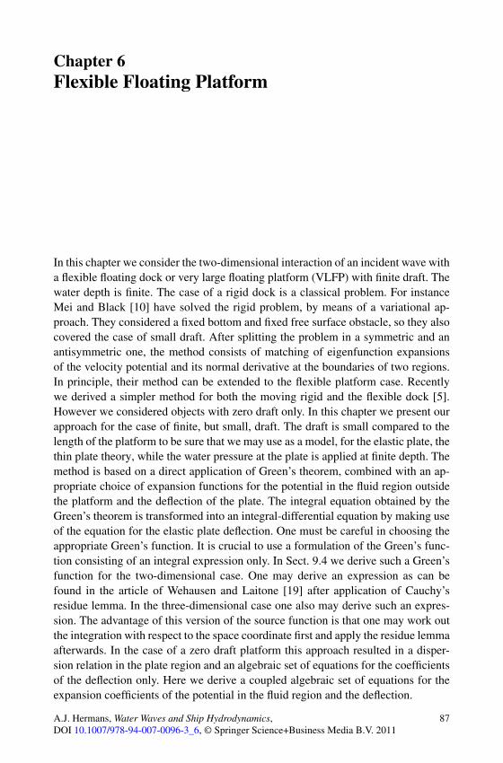
Chapter 6Flexible Floating Platform
In this chapter we consider the two-dimensional interaction of an incident wave witha flexible floating dock or very large floating platform (VLFP) with finite draft. Thewater depth is finite. The case of a rigid dock is a classical problem. For instanceMei and Black [10] have solved the rigid problem, by means of a variational ap-proach. They considered a fixed bottom and fixed free surface obstacle, so they alsocovered the case of small draft. After splitting the problem in a symmetric and anantisymmetric one, the method consists of matching of eigenfunction expansionsof the velocity potential and its normal derivative at the boundaries of two regions.In principle, their method can be extended to the flexible platform case. Recentlywe derived a simpler method for both the moving rigid and the flexible dock [5].However we considered objects with zero draft only. In this chapter we present ourapproach for the case of finite, but small, draft. The draft is small compared to thelength of the platform to be sure that we may use as a model, for the elastic plate, thethin plate theory, while the water pressure at the plate is applied at finite depth. Themethod is based on a direct application of Green’s theorem, combined with an ap-propriate choice of expansion functions for the potential in the fluid region outsidethe platform and the deflection of the plate. The integral equation obtained by theGreen’s theorem is transformed into an integral-differential equation by making useof the equation for the elastic plate deflection. One must be careful in choosing theappropriate Green’s function. It is crucial to use a formulation of the Green’s func-tion consisting of an integral expression only. In Sect. 9.4 we derive such a Green’sfunction for the two-dimensional case. One may derive an expression as can befound in the article of Wehausen and Laitone [19] after application of Cauchy’sresidue lemma. In the three-dimensional case one also may derive such an expres-sion. The advantage of this version of the source function is that one may work outthe integration with respect to the space coordinate first and apply the residue lemmaafterwards. In the case of a zero draft platform this approach resulted in a disper-sion relation in the plate region and an algebraic set of equations for the coefficientsof the deflection only. Here we derive a coupled algebraic set of equations for theexpansion coefficients of the potential in the fluid region and the deflection.
A.J. Hermans, Water Waves and Ship Hydrodynamics,DOI 10.1007/978-94-007-0096-3_6, © Springer Science+Business Media B.V. 2011
87

88 6 Flexible Floating Platform
6.1 The Finite Draft Problem
In this section we derive the general formulation for the diffraction of waves bya flexible platform of general geometric form. The fluid is ideal, so we introducea velocity potential using V(x, t) = ∇�(x, t), where V(x, t) is the fluid velocityvector. Hence �(x, t)is a solution of the Laplace equation
�� = 0 in the fluid, (6.1)
together with the linearised kinematic condition, �y = vt , and dynamic condition,p/ρ = −�t − gv, at the mean water surface y = 0, where v(x, z, t) denotes thefree surface elevation, and ρ is the density of the water. The linearised free surfacecondition outside the platform, y = 0 and (x, z) ∈ F , becomes
∂2�
∂t2+ g
∂�
∂y= 0. (6.2)
The platform is situated at the mean free-surface y = 0, its thickness is d . The plat-form is modelled as an elastic plate with zero thickness. The neutral axis of the plateis at y = 0, while the water pressure distribution is applied at y = −d . Meylan etal. [11] have considered finite thickness as well. They consider the elastic equationfor the deflection of a plate of finite thickness, however they apply the equationof motion at y = 0. They show for large platforms a minor influence due to thechange of the elastic model. Our elastic model can easily be modified by changingthe fourth-order differential operator, but due to lack of knowledge of suitable pa-rameters we decided not to do so. So we neglect horizontal and torsional motion. Todescribe the vertical deflection v(x, z, t), we apply the isotropic thin-plate theory,which leads to an equation for v of the form
m(x, z)∂2v
∂t2= −
(∂2
∂x2+ ∂2
∂z2
)(D(x, z)
(∂2v
∂x2+ ∂2v
∂z2
))+ p|y=−d (6.3)
where m(x, z) is the piece-wise constant mass of unit area of the platform while thepiece-wise constant D(x, z) is its equivalent flexural rigidity. We differentiate (6.3)with respect to t and use the kinematic and dynamic condition to arrive at the fol-lowing equation for � at y = −d in the platform area (x, z) ∈ P :
{(∂2
∂x2+ ∂2
∂z2
)(D(x, z)
ρg
(∂2
∂x2+ ∂2
∂z2
))+ m(x, z)
ρg
∂2
∂t2+ 1
}∂�
∂y
+ 1
g
∂2�
∂t2= 0. (6.4)
Due to the fact that the plate is freely floating we do not consider the hydrostaticpressure.

6.1 The Finite Draft Problem 89
The edges of the platform are free of shear forces and moment. We assume thatthe flexural rigidity is constant along the edge and its derivative normal to the edgeequals zero. Also, we assume that the radius of curvature, in the horizontal plane, ofthe edge is large. Hence, the edge may be considered to be straight locally. We thenhave the following boundary conditions at the edge:
∂2v
∂n2+ ν
∂2v
∂s2= 0 and
∂3v
∂n3+ (2 − ν)
∂3v
∂n∂s2= 0 (6.5)
where ν is Poisson’s ratio, n is in the normal direction, in the horizontal plane,along the edge and s denotes the arc-length along the edge. At the bottom of thefluid region y = −h we have
∂�
∂y= 0. (6.6)
We assume that the velocity potential is a time-harmonic wave function, �(x, t) =φ(x)eiωt . We introduce the following parameters:
K = ω2
g, μ = mω2
ρg, D = D
ρg.
In a practical situation the total length L of the platform is a few thousand metres.We obtain at the free surface, y = 0,
∂φ
∂z− Kφ = 0 (6.7)
and at the plate, y = −d , for a single strip,
{D
(∂2
∂x2+ ∂2
∂z2
)2
− μ + 1
}∂φ
∂y− Kφ = 0. (6.8)
The potential of the undisturbed incident wave is given by
φinc(x) = gη∞iω
cosh(k0(y + h))
cosh(k0h)exp{ik0(x cosβ + z sinβ)} (6.9)
where η∞ is the wave amplitude in the original coordinate system, ω the frequency,while the wave number k0 is the negative real solution of the dispersion relation
k0 tanh(k0h) = K, (6.10)
for finite water depth. We restrict ourselves to the case of normal incidence, β = 0.In [6] is shown that the extension to oblique waves can be done easily.
To obtain an integral equation for the deflection v(x, z, t) = �[v(x, z)eiωt ] of theplatform, see [4, 6], it is very convenient to apply the Green’s theorem, making useof the Green’s function, G (x;ξξξ), that fulfils boundary conditions at the seabed (6.6)

90 6 Flexible Floating Platform
and at the free surface (6.7). Application of Green’s theorem in the fluid domainleads to the following expression for the potential function:
4πφ(x) = 4πφinc(x) +∫
Cφ(ξξξ)
∂G (x,ξξξ)
∂ndS
+∫
P
(φ(ξξξ)
∂G (x,ξξξ)
∂η− ∂φ(ξξξ)
∂ηG (x;ξξξ)
)dS. (6.11)
The first integral is along the vertical sides of the platform, where the normal ve-locity of the fluid equals zero. The second integral is along the flat bottom. In thetwo-dimensional case, (x, y)-plane, the expression for the total potential becomes
2πφ(x, y) = 2πφinc(x, y)
+∫ 0
−d
(φ(0, η)
∂G (x, y;0, η)
∂ξ− φ(l, η)
∂G (x, y; l, η)
∂ξ
)dη
+∫ l
0
(φ(ξ,−d)
∂G (x, y; ξ,−d)
∂η− ∂φ(ξ,−d)
∂ηG (x, y; ξ,−d)
)dξ.
(6.12)
We continue with the two-dimensional case.The Green’s function G(x,y; ξ, η) for the two dimensional case can be derived
by means of a Fourier transform with respect to the x-coordinate. As is shown inSect. 9.4 it has the form:
G(x,y; ξ, η) =∫ ∞
−∞1
γ
K sinhγy + γ coshγy
K coshγ h − γ sinhγ hcoshγ (η + h)eiγ (x−ξ) dγ
for y > η (6.13)
and
G(x, z; ξ, η) =∫ ∞
−∞1
γ
K sinhγ η + γ coshγ η
K coshγ h − γ sinhγ hcoshγ (y + h)eiγ (x−ξ) dγ
for y < η. (6.14)
If we close the contour of integration in the complex γ -plane we obtain the complexversion of formula (13.34), as can be found in Wehausen and Laitone [19]
G(x, z; ξ, η) = −2π i∞∑i=0
1
ki
k2i − K2
hk2i − hK2 + K
coshki(y + h) cosh ki(η + h)eiki |x−ξ |,
(6.15)where k0 and ki, i = 1, . . . ,∞ are the positive real and positive imaginary zeros ofthe dispersion relation (6.10).
The advantage of this formulation for the Green’s function is that, by means ofthe Green’s theorem, we can derive an algebraic set of equations for the expansion
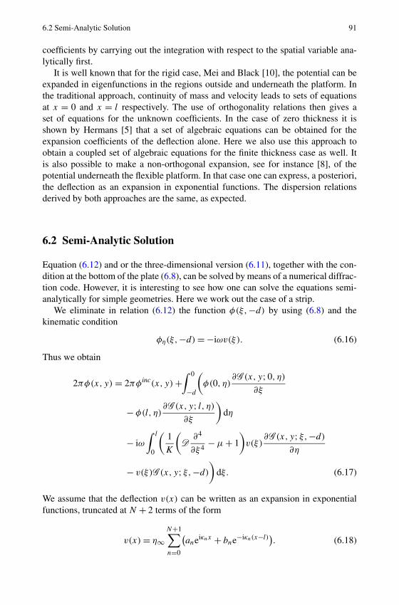
6.2 Semi-Analytic Solution 91
coefficients by carrying out the integration with respect to the spatial variable ana-lytically first.
It is well known that for the rigid case, Mei and Black [10], the potential can beexpanded in eigenfunctions in the regions outside and underneath the platform. Inthe traditional approach, continuity of mass and velocity leads to sets of equationsat x = 0 and x = l respectively. The use of orthogonality relations then gives aset of equations for the unknown coefficients. In the case of zero thickness it isshown by Hermans [5] that a set of algebraic equations can be obtained for theexpansion coefficients of the deflection alone. Here we also use this approach toobtain a coupled set of algebraic equations for the finite thickness case as well. Itis also possible to make a non-orthogonal expansion, see for instance [8], of thepotential underneath the flexible platform. In that case one can express, a posteriori,the deflection as an expansion in exponential functions. The dispersion relationsderived by both approaches are the same, as expected.
6.2 Semi-Analytic Solution
Equation (6.12) and or the three-dimensional version (6.11), together with the con-dition at the bottom of the plate (6.8), can be solved by means of a numerical diffrac-tion code. However, it is interesting to see how one can solve the equations semi-analytically for simple geometries. Here we work out the case of a strip.
We eliminate in relation (6.12) the function φ(ξ,−d) by using (6.8) and thekinematic condition
φη(ξ,−d) = −iωv(ξ). (6.16)
Thus we obtain
2πφ(x, y) = 2πφinc(x, y) +∫ 0
−d
(φ(0, η)
∂G (x, y;0, η)
∂ξ
− φ(l, η)∂G (x, y; l, η)
∂ξ
)dη
− iω∫ l
0
(1
K
(D
∂4
∂ξ4− μ + 1
)v(ξ)
∂G (x, y; ξ,−d)
∂η
− v(ξ)G (x, y; ξ,−d)
)dξ. (6.17)
We assume that the deflection v(x) can be written as an expansion in exponentialfunctions, truncated at N + 2 terms of the form
v(x) = η∞N+1∑n=0
(aneiκnx + bne−iκn(x−l)
). (6.18)
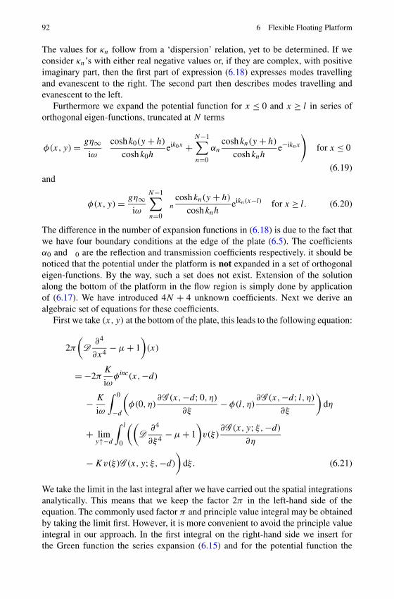
92 6 Flexible Floating Platform
The values for κn follow from a ‘dispersion’ relation, yet to be determined. If weconsider κn’s with either real negative values or, if they are complex, with positiveimaginary part, then the first part of expression (6.18) expresses modes travellingand evanescent to the right. The second part then describes modes travelling andevanescent to the left.
Furthermore we expand the potential function for x ≤ 0 and x ≥ l in series oforthogonal eigen-functions, truncated at N terms
φ(x, y) = gη∞iω
(cosh k0(y + h)
cosh k0heik0x +
N−1∑n=0
αn
coshkn(y + h)
cosh knhe−iknx
)for x ≤ 0
(6.19)and
φ(x, y) = gη∞iω
N−1∑n=0
βn
cosh kn(y + h)
cosh knheikn(x−l) for x ≥ l. (6.20)
The difference in the number of expansion functions in (6.18) is due to the fact thatwe have four boundary conditions at the edge of the plate (6.5). The coefficientsα0 and β0 are the reflection and transmission coefficients respectively. it should benoticed that the potential under the platform is not expanded in a set of orthogonaleigen-functions. By the way, such a set does not exist. Extension of the solutionalong the bottom of the platform in the flow region is simply done by applicationof (6.17). We have introduced 4N + 4 unknown coefficients. Next we derive analgebraic set of equations for these coefficients.
First we take (x, y) at the bottom of the plate, this leads to the following equation:
2π
(D
∂4
∂x4− μ + 1
)(x)
= −2πK
iωφinc(x,−d)
− K
iω
∫ 0
−d
(φ(0, η)
∂G (x,−d;0, η)
∂ξ− φ(l, η)
∂G (x,−d; l, η)
∂ξ
)dη
+ limy↑−d
∫ l
0
((D
∂4
∂ξ4− μ + 1
)v(ξ)
∂G (x, y; ξ,−d)
∂η
− Kv(ξ)G (x, y; ξ,−d)
)dξ. (6.21)
We take the limit in the last integral after we have carried out the spatial integrationsanalytically. This means that we keep the factor 2π in the left-hand side of theequation. The commonly used factor π and principle value integral may be obtainedby taking the limit first. However, it is more convenient to avoid the principle valueintegral in our approach. In the first integral on the right-hand side we insert forthe Green function the series expansion (6.15) and for the potential function the

6.2 Semi-Analytic Solution 93
expansions (6.19) and (6.20), while in the second integral we use (6.14) for theGreen function and (6.18) for the deflection. In the first integral integration withrespect to η and in the last integral the integration with respect to ξ can be carriedout. Next we close the remaining contour of integration in the complex γ -plane.
If we now equalise the coefficients of eiκnx and of e−iκn(x−l), we obtain the fol-lowing ‘dispersion’ relation for κn, the κn’s are the zero’s of
(Dκ4 − μ)K coshκd + (K2 − κ2(Dκ4 − μ + 1))sinhκd
κ
= (Dκ4 − μ + 1)(K coshκh − κ sinhκh)
coshκ(−d + h).
After some manipulations this relation can be rewritten in the form
((Dκ4 − μ − 1)κ tanhκ(h − d) − K)(K sinhκd − κ coshκd) = 0. (6.22)
For d = 0 the dispersion relation for the zero draft platform is recovered. It shouldbe noticed that relation (6.22) is not exactly the same as the zero draft relation withh replaced by h− d . Hence, we ignore the zeros of the second part, which occur forvalues of K sufficiently large only.
6.2.1 Semi-Infinite Platform
Let us first consider the half-plane problem. We introduce some slight physicaldamping to get rid of the contributions of the upper bound in the last integralin (6.21) and the second part of the first integral. The terms we obtain after clo-sure of the contour in the last integral of (6.21) contain the exponential functionseiknx . We take the coefficients of each exponential equal to zero. This leads to a setof N algebraic equations for the coefficients an and αn. For the half-plane problem,we obtain for i = 0, . . . ,N − 1:
N−1∑n=0
αn
cosh knhKi,n −
N+1∑n=0
an
κn − ki
((Dκ4
n − μ + 1) sinhki(h − d)
− K
ki
coshki(h − d)
)
= δ0i
hk20 − hK2 + K
(k20 − K2) coshk0h)
− Ki,0
coshk0h, (6.23)
where the coefficients Ki,n are defined as
2Ki,n = 1
ki + kn
[sinh(ki + kn)h − sinh(ki + kn)(h − d))]
+ 1
ki − kn
[sinh(ki − kn)h − sinh(ki − kn)(h − d)]. (6.24)

94 6 Flexible Floating Platform
This is a set of N equations for 2N + 2 unknown coefficients. We have two condi-tions at the edge of the plate, so we must still obtain N . At the vertical front end ofthe platform (6.17) gives the relation
2πφ(0, y) = 2πφinc(0, y) + limx→0
∫ 0
−d
φ(0, η)∂G (x, y;0, η)
∂ξdη
− iω∫ ∞
0
(1
K
(D
∂4
∂ξ4− μ + 1
)v(ξ)
∂G (0, y; ξ,−d)
∂η
− v(ξ)G (0, y; ξ,−d)
)dξ. (6.25)
We insert the series expansions (6.18) and (6.19) in this equation and compare thecoefficients of coshki(y + h). For the Green function we use expression (6.15) inboth integrals.
We obtain for i = 0, . . . ,N − 1,
hk2i − hK2 + K
(k2i − K2) cosh kih
αi −N−1∑n=0
αn
coshknhKi,n
−N+1∑n=0
an
κn + ki
((Dκ4
n − μ + 1) sinhki(h − d) − K
ki
cosh ki(h − d)
)
= 1
cosh k0hKi,0. (6.26)
We give some results for the absolute value of the amplitude of the deflection fora semi-infinite platform with a draft of two metres and water depth of ten me-tres. In Fig. 6.1 results are shown for three values of the deep water wave length,λ = 2π/K = 150,90,30 m respectively. As expected the amplitude increases withincreasing values of the wave length. In Fig. 6.2 we show for λ = 90 m and waterdepth of ten metre the absolute value of the amplitude for several values of the draft,d = 0,2,4,6 m. In Fig. 6.3 we show the influence of water depth on the amplitude ofdeflection. We have chosen h = 100,20,10 m, d = 2 m and a fixed frequency withλ = 90 m. The amplitude of the deflection increases for increasing water depth. Tocarry out computations for the larger values of water depth one must get rid of allhyperbolic sin and cosine functions in the formulation. This can be done by usingstandard formulas for these functions and by using the dispersion relation for thefree surface water waves. By doing so one obtains very accurate results. In Fig. 6.4we show the real part of the deflection for the same values of water depth, d = 5 mand fixed values of the wavelength λ0 = 2π/k0 = 100 m. We also have computedthe absolute value of the amplitude of the wave elevation in front of the platform.The result is shown in Fig. 6.5. It is clearly shown that the elevation of the waveand the platform are discontinuous at x = 0. The amplitude of the reflected waveα0 = 0.45657 − 0.43639i.
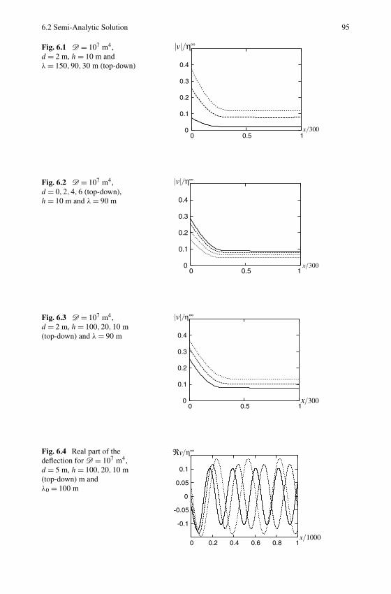
6.2 Semi-Analytic Solution 95
Fig. 6.1 D = 107 m4,d = 2 m, h = 10 m andλ = 150,90,30 m (top-down)
Fig. 6.2 D = 107 m4,d = 0,2,4,6 (top-down),h = 10 m and λ = 90 m
Fig. 6.3 D = 107 m4,d = 2 m, h = 100,20,10 m(top-down) and λ = 90 m
Fig. 6.4 Real part of thedeflection for D = 107 m4,d = 5 m, h = 100,20,10 m(top-down) m andλ0 = 100 m

96 6 Flexible Floating Platform
Fig. 6.5 Amplitude of waveand deflection forD = 107 m4, d = 2 m,h = 10 m and λ = 90 m
6.2.2 Strip of Finite Length
We follow the same procedure as for the semi-infinite case. The first step is to com-pare the coefficients of the exponential functions e±iknx in (6.21). This leads to a setof 2N algebraic equations for the coefficients an, bn,αn and βn.
N−1∑n=0
αn
cosh knhKi,n
−N+1∑n=0
an
κn − ki
((Dκ4
n − μ + 1) sinhki(h − d) − K
ki
cosh ki(h − d)
)
+N+1∑n=0
bn
κn + ki
((Dκ4
n − μ + 1) sinhki(h − d) − K
ki
cosh ki(h − d)
)eiκnl
= δ0i
hk20 − hK2 + K
(k20 − K2) coshk0h)
− Ki,0
coshk0h(6.27)
and
N−1∑n=0
βn
cosh knhKi,n
+N+1∑n=0
an
κn + ki
((Dκ4
n − μ + 1) sinh ki(h − d) − K
ki
coshki(h − d)
)eiκnl
−N+1∑n=0
bn
κn + ki
((Dκ4
n − μ + 1) sinh ki(h − d) − K
ki
coshki(h − d)
)= 0.
(6.28)
This is a set of 2N equations for 4N + 4 unknown coefficients. Next we considerthe equations at x = 0 and x = l respectively. After integration with respect to thespatial variable one obtains a summation of cosh ki(y + h) terms. By taking thecoefficients of each coshki(y + h) function equal to zero we obtain the followingset of 2N equations for the unknown expansion coefficients.

6.2 Semi-Analytic Solution 97
At x = 0 we get
hk2i − hK2 + K
(k2i − K2) cosh kih
αi −N−1∑n=0
αn − βneiki l
cosh knhKi,n
−N+1∑n=0
an
κn + ki
((Dκ4
n − μ + 1) sinhki(h − d) − K
ki
cosh ki(h − d)
)
× (1 − ei(κn+ki )l
)
+N+1∑n=0
bn
κn − ki
((Dκ4
n − μ + 1) sinhki(h − d) − K
ki
cosh ki(h − d)
)
× (eiκnl − eiki l
)
= 1
cosh k0hKi,0, (6.29)
and at x = l we get
hk2i − hK2 + K
(k2i − K2) cosh kih
βi +N−1∑n=0
αneiki l − βn
cosh knhKi,n
+N+1∑n=0
an
κn − ki
((Dκ4
n − μ + 1) sinhki(h − d) − K
ki
cosh ki(h − d)
)
× (eiκnl − eiki l
)
−N+1∑n=0
bn
κn + ki
((Dκ4
n − μ + 1) sinhki(h − d) − K
ki
cosh ki(h − d)
)
× (1 − ei(κn+ki )l
)
= hk20 − hK2 + K
(k20 − K2) cosh k0h
eik0l − 1
cosh k0hKi,0. (6.30)
Together with the four relations at the end of the strip we have 4N + 4 linear alge-braic equations for the 4N + 4 unknown coefficients.
The set of equations as is written here is not very suitable for numerical com-putations directly. Especially for large values of water-depth the arguments of thehyperbolic sine and cosine functions become rather large. So one is subtracting verylarge values in the computation of the coefficients. To obtain high numerical accu-racy one must get rid of these functions. This can be done by using the dispersionrelation for the water region. In Sect. 9.5 a more suitable set of equations is given.
We show some computational results for a two-dimensional platform of width300 m. In all cases we take a fixed value for the flexural rigidity D = 107 m4, the

98 6 Flexible Floating Platform
Fig. 6.6 D = 107 m4,l = 300 m, d = 0 m,h = 10 m andλ/l = 0.5, . . . ,0.3,−−,0.1,−−
Fig. 6.7 D = 107 m4,l = 300 m, d = 2 m,h = 10 m andλ/l = 0.5,0.3,0.1
width of the strip l = 300 m and the water depth h = 10 m. In Figs. 6.6 and 6.7 weshow for d = 0 and for d = 2 m the variation of the amplitude of deflection withrespect to the wave length. In Figs. 6.8 and 6.9 the dependence on the draft for fixedvalues of the wave length is shown. The results of the first case show an increaseof the deflection for increasing values of the draft. It will be shown later that thisis due to a shift in the reflection curve. In Fig. 6.10 a result is shown for a largervalue of the flexural rigidity D = 1010 m4 and wave length λ/l = 0.5. This case iscomparable with the interaction of free-surface waves with a rigid body. One clearlyobserves that the motion of the dock consists of a heave and pitch motion only.
In Figs. 6.11 and 6.13 we show for two values of the wave length the absolutevalue of the amplitude of the water surface in front of and behind the strip, togetherwith the amplitude of the plate deflection for the zero draft case. The second case isnear the zero reflection situation. In the four metre draft case, see Figs. 6.12 and 6.14,we see that λ/l = 0.215, or in terms of the actual wave length λ0/l = 0.178, is closeto total reflection. This is in contrast with the zero draft case in Fig. 6.13, due to theshift in the transmission-reflection curves. For the same reason the absolute value ofthe deflection increases if the draft increases in Fig. 6.8 in contrast with the result inFig. 6.9.
The reflection and transmission coefficients for a strip of 300 m and depth 10 mare shown in Fig. 6.15, for zero draft and in Fig. 6.16 for a draft of 2 meteors. If wedefine R = α0 and T = β0, notice no exponential function, we find that in all casesthe relations |T |2 + |R|2 = 1 and T R + T R = 0, see for instance Mei et al. [10] orfor a derivation Roseau [16], are fulfilled for at least 10 decimals. The coefficientsare presented as a function of the actual wave length, λ0/l = 2π/k0l. In Figs. 6.17

6.2 Semi-Analytic Solution 99
Fig. 6.8 D = 107 m4,l = 300 m, d = 0,−−,2,−−,4, . . . m, h = 10 mand λ/l = 0.3
Fig. 6.9 D = 107 m4,l = 300 m, d = 0,−−,2,−−,4, . . . m, h = 10 mand λ/l = 0.5
Fig. 6.10 D = 1010 m4,l = 300 m, d = 0,2,4 m,h = 10 m and λ/l = 0.5
Fig. 6.11 D = 107 m4,l = 300 m, d = 0 m,h = 10 m and λ/l = 0.3

100 6 Flexible Floating Platform
Fig. 6.12 D = 107 m4,l = 300 m, d = 4 m,h = 10 m and λ/l = 0.3
Fig. 6.13 D = 107 m4,l = 300 m, d = 0 m,h = 10 m and λ/l = 0.215
Fig. 6.14 D = 107 m4,l = 300 m, d = 4 m,h = 10 m and λ/l = 0.215
Fig. 6.15 −−− Reflectionand −− transmissioncoefficients for h = 10 m,d = 0 m and l = 300 m

6.2 Semi-Analytic Solution 101
Fig. 6.16 Reflection andtransmission coefficients forh = 10 m, d = 4 m andl = 300 m
Fig. 6.17 Reflection andtransmission coefficients forh = 100 m, d = 0 m andl = 300 m
Fig. 6.18 Reflection andtransmission coefficients forh = 100 m, d = 2 m, andl = 300 m
Fig. 6.19 Reflection andtransmission coefficients forh = 100 m, d = 2 m, andl = 650 m

102 6 Flexible Floating Platform
Fig. 6.20 Reflection andtransmission coefficients forh = 100 m, d = 2 m andl = 1000 m
Fig. 6.21 Reflection andtransmission coefficients forh = 100 m, d = 8 m, andl = 1000 m
Fig. 6.22 Reflection andtransmission coefficients forh = 500 m, d = 8 m andl = 1000 m
and 6.18 these coefficients are given for a water depth of 100 metres. In all cases thecoefficient of flexural rigidity equals D = 107 m4. Figures 6.18, 6.19 and 6.20 showthe results for different sizes of the strip. In Figs. 6.21 and 6.22 the result is shownfor a strip of width l = 100 m and draft d = 8 m. It is clearly observed that for theshort waves total reflection takes place.

Chapter 7Irregular and Non-linear Waves
The surface waves of the sea are almost always random in the sense that detailedconfiguration of the surface varies in an irregular manner in both space and time.Section 7.1 contains a brief description of the Wiener spectrum in connection withthe generalised Fourier representations for the surface waves [2, 20]. In this waywe see how one may represent the surface elevation by a superposition of harmonicwaves with amplitudes being a stochastic process.
The remaining sections in the chapter are devoted to non-linear waves. InSect. 7.2 we give a systematic derivation of the shallow water theory from the exacthydrodynamical equations as the approximation of lowest order in a perturbationprocedure. Here the relevant small parameter is the ratio of the depth of water tosome characteristic length associated with the horizontal direction such as the wavelength; the water is considered shallow when this parameter is small. It is a differentkind of approximation from the previous linear theory for waves of small amplitude.The resulting equations here are quasi-linear and are exactly analogous to the onesin gas dynamics. Second order approximations are included in the last Sect. 7.3. Inparticular, an asymptotic theory will be developed for slowly varying wave trains,which may be considered as nearly uniform in the regions of order of magnitudeof a small number of wave lengths and periods. Some non-linear dispersive wavephenomena will be discussed and more details can be found in [7].
7.1 Wiener Spectrum
The actual motion of the sea is by no means a harmonic motion with constant fre-quency. In Sect. 2.1.2, we gave a representation of the sea surface η(x, t) in the formof an integral*
η(x, t) =∫ ∞
−∞{A(k)e−i(kx−ωt) + A∗(k)ei(kx−ωt)
}dk
under the hypothesis that∫ ∞− ∞|A(k)|2 dk is convergent. It is, however, not ap-
propriate to suppose that the amplitudes of the high frequencies go to zero. The
A.J. Hermans, Water Waves and Ship Hydrodynamics,DOI 10.1007/978-94-007-0096-3_7, © Springer Science+Business Media B.V. 2011
103

104 7 Irregular and Non-linear Waves
representation by a Fourier integral there breaks down and we must use a theorydeveloped by Wiener of which we shall give an outline below. Details can be foundin Wiener’s book [20] in the references.
For a better understanding, we begin with a trigonometric polynomial f (t) de-fined by
f (t) =n∑
j=1
Aj eiλj t ,
and calculate
f (t + τ)f ∗(t) =n∑
j=1
n∑k=1
AjA∗keiλj tei(λj −λk)τ .
Here A∗k again denotes the complex conjugate of Ak . Now by taking the averaged
mean of this quantity, we obtain that
limT →∞
1
2T
∫ T
−T
f (t + τ)f ∗(τ )dτ =n∑
j=1
n∑k=1
AjA∗keiλj t lim
T →∞1
2T
∫ T
−T
ei(λj −λk)τ dτ.
For λj = λk , the limit is equal to unity, but for λj �= λk , the limit vanishes. Thisleads to the result
limT →∞
1
2T
∫ T
−T
f (t + τ)f ∗(τ )dτ =n∑
j=1
|Aj |2eiλt .
In other words, if we put
ϕ(t) = limT →∞
1
2T
∫ T
−T
f (t + τ)f ∗(τ )dτ,
then ϕ(t) exists for every t , is continuous and consists of terms with the same fre-quency as those constituting f (t) and with amplitudes equal to the square of theamplitudes of the corresponding terms of f (t). Hence we see a way of finding aFourier integral representation of a function which does not vanish at infinity. Onecan analyse the surface waves by means of functions of this kind in space variablesas well as in the time variable.
We next build up the Wiener theory for those complex functions f (t) of he realvariable t such that
ϕ(t) = limT →∞
1
2T
∫ T
−T
f (t + τ)f ∗(τ )dτ, (7.1)
exists for all t . Clearly then ϕ(0) also exists. This means that the quadratic mean ofthe function exists. Moreover from the Schwartz’s inequality, it can be shown thatfor all real t ,
|ϕ(t)| ≤ ϕ(0).

7.1 Wiener Spectrum 105
Indeed, it is easy to see that
|ϕ(t)| = limT →∞
∣∣∣∣ 1
2T
∫ T
−T
f (t + τ)f ∗(τ )dτ
∣∣∣∣≤
{lim
T →∞1
2T
∫ T +|t |
−T −|t ||f (τ)|2 dτ lim
T →∞1
2T
∫ T
−T
|f (τ)|2 dτ
}1/2
≤{(
limT →∞
T + |t |T
)(lim
T →∞1
2(T + |t |)∫ T +|t |
−T −|t ||f (τ)|2 dτ
)
·(
limT →∞
1
2T
∫ T
−T
|f (τ)|2 dτ
)}1/2
= {1 × ϕ(0) × ϕ(0)
}1/2 = ϕ(0).
Here we use the notation lim = lim sup for the limit superior. Recall thatlimSn = A ⇐⇒ the sequence {Sn}∞n=1 is bounded above and has A as its largestlimit point.
We now try to define a reasonable Fourier transform for those functions f (t)
in (7.1). Clearly from (7.1), the standard Fourier transform for f (t),1√2π
∫ ∞−∞ f (τ)e−iωτ dτ , need not exist but the limit
limT →∞
∫ T
−T
f (τ)eiωτ dτ
does exist. This leads us to consider the integral
∫ ∞
−∞eiωt
itdt,
although the integrand is singular at t = 0. Since ϕ(0) exists it follows that
1
2T
∫ T
−T
|f (t)|2 dt
is bounded in T and hence the function which is f (t)/it for |t | > 1 and 0 for t ≤ 1belongs to L2, consequently its Fourier transform (in L2) exists and belongs to L2.Thus we define
S(ω) = 1√2π
l.i.m.A→∞
[∫ −1
−A
+∫ A
1
]f (t)e−iωt
−itdt + 1√
2π
∫ 1
−1
e−iωt − 1
−itdt, (7.2)
and consider the difference S(ω + ε) − S(ω − ε) which can be reduced to
S(ω + ε) − S(ω − ε) = 1√2π
l.i.m.A→∞
∫ A
−A
f (t)2 sin εt
te−ıωt dt. (7.3)

106 7 Irregular and Non-linear Waves
Here and in the sequel we use the notation for the limit in the mean:l.i.m.a→a0gα(ω) = g(ω) if
limα→α0
∫ ∞
−∞|gα(ω) − g(ω)|2 dω = 0,
where α0 is any fixed constant including ∞. Because of our assumption for f (t)
in (7.1), clearly S(ω) in (7.2) exists and so is due to the difference S(ω + ε) −S(ω − ε) in (7.3), which is the ordinary Fourier transform of f (t) 2 sin εt
t. Here S(ω)
as defined by (7.2) is termed as the generalised Fourier transform of f (t).At this stage, Wiener uses a Tauberian therem: If ϕ(t) ≥ 0 for 0 ≤ t < ∞, and
either of the limits
limT →∞
1
T
∫ T
0ϕ(t)dt or lim
ε→0
2
πε
∫ ∞
0ϕ(t)
sin2(εt)
t2dt
exists, then the other limit exists and assumes the same value. Wiener’s proof of thistheorem is very complicated. However as a corollary, we have the result that
limε→0
1
4πε
∫ ∞
−∞|S(ω + ε) − S(ω − ε)|2 dω = lim
T →∞1
2T
∫ T
−T
|f (t)|2 dt.
We now define Sτ (ω), which bears the same relation to f (t + τ) as S(ω) to f (t)
in (7.2). Then we have
Sτ (ω + ε) − Sτ (ω − ε) − eiτω{S(ω + ε) − S(ω − ε)
}
= 1√2π
{l.i.m.A→∞
∫ A
−A
f (t + τ)2 sin(εt)
te−iεt dt
− l.i.m.A→∞
∫ A
−A
f (t + τ)2 sin(εt)
te−iε(t−τ) dt
}.
This can be transformed into
1√2π
l.i.m.A→∞
∫ A
−A
f (t)
[2 sin(ε(t − τ))
t − τ− 2 sin(εt)
t
]e−iω(t−τ) dt.
Thus from the Plancherel theorem, it follows that∫ ∞
−∞∣∣Sτ (ω + ε) − Sτ (ω − ε) − eiωτ
{S(ω + ε) − S(ω − ε)
}∣∣2 dω
=∫ ∞
−∞|f (t)|2
[2 sin((t − τ)ε)
t − τ− 2 sin(tε)
t
]2
dt.
Now it can be shown that∣∣∣∣2 sin((t − τ)ε)
t − τ− 2 sin(tε)
t
∣∣∣∣ ≤ 16ε|τ ||t | + |τ | ,
7.1 Wiener Spectrum 107
and hence by the Tauberian theorem and the fact that if 12T
∫ T
−t|f (t)|2 dt is bounded
in T , then∫ ∞−∞ |f (t)|2/(1 + t2)dt < ∞ and we have
∫ ∞
−∞
∣∣∣∣Sτ (ω + ε) − Sτ (ω − ε) − eiωτ
{S(ω + ε) − S(ω − ε)
}∣∣∣∣2
dω = O(ε2).
Then from this, Wiener derives that
ϕ(τ) = limε→0
1
4πε
∫ ∞
−∞eiωτ
∣∣S(ω + ε) − S(ω − ε)∣∣2 dω. (7.4)
Putting
ϕε(τ ) = 1
4πε
∫ ∞
−∞eiωτ
∣∣S(ω + ε) − S(ω − ε)∣∣2 dω,
Wiener shows that the function
σε(ω) := 1√2π
{l.i.m.A→∞
[∫ A
1+
∫ −1
−A
]ϕε(t)e−iωt
−itdt +
∫ 1
−1ϕε(t)
e−iωt − 1
−itdt
}
is equal to
constant + 1
2ε√
2π
∫ ∞
0|S(ω′ + ε) − S(ω′ − ε)|2 dω′.
Or, with σ(ω) = l.i.m.ε→0σε(ω), we have
σ(ω) − σ(−ω) = 1
2ε√
2πl.i.m.ε→0
∫ ω
−ω
|S(ω′ + ε) + −S(ω′ − ε)|2 dω′. (7.5)
Finally, Wiener shows that
ϕ(τ) = 1√2π
∫ ∞
−∞eiτω dσ(ω). (7.6)
If we let F(ω) 1√2π
(σ (ω) − σ(−ω)), then (7.6) can be written as
ϕ(τ) =∫ ∞
0cos(ωτ)dF(ω). (7.7)
In this way we have introduced the spectral function F(ω) of f (t) and have estab-lished the generalised Fourier representation. It should be noted that this conceptjust follows from the assumption of the existence of the auto-correlation functionof f (t) defined by
limT →∞
1
2T
∫ T
−T
f (t + τ)f ∗(t)dt,

108 7 Irregular and Non-linear Waves
which has been denoted by ϕ(τ) (cf. (7.1)). This auto-correlation function ϕ(τ) isfound by a summation of contributions of the different frequencies of the spectrum.This leads to consider the function f (t) as a realisation of a stochastic process,consisting of a superposition of different harmonic waves, the amplitudes of whichare random variables of ω.
We first remark that if f (t) is a stationary process of second order,1 with theunderstanding that the process is a centred process, i.e., E{f (t)} = 0, there existsa covariance function E{f (t + τ)f ∗(t)} which is independent of t for a stationaryprocess. If the process is ergodic, then this covariance function is equal to the auto-correlation ϕ(t), i.e.,
E{f (t + τ)f ∗(t)} = limT →∞
1
2T
∫ T
−T
f (t + τ)f ∗(t)dt. (7.8)
This means that from the relation (7.7), we can consider the process f (t) as a su-perposition of the stochastic process A(ω), which consists of functions of the fre-quency ω with independent increments in such a way that E{dA(ω)dA∗(ω)} = 0,if dω �= dω′. Thus, if we put dF(ω) = 2E{dA(ω)dA∗(ω)}, we can express f (t) as
f (t) =∫ ∞
−∞eiωt dA(ω). (7.9)
In the case of surface waves, we have the vector xxx = (x, y) and the representationtakes the form of a superposition of plane waves as a stochastic integral,
η(x, y, t) =∞∫∫
−∞ei(k·xk·xk·x−iωt) dA(kkk), (7.10)
where ω and kkk = (k1, k2) are related by the dispersion relation ω = H(kkk). The en-ergy spectrum is given by dF = E{dA(kkk)dA∗(kkk)}. The energy spectrum depends
on both the wave number k =√
k21 + k2
2 and the direction ϑ such that k1 = k cosϑ
and k1 = k sinϑ . We denote it by dF(k,ϑ).In Sect. 3.2.4 we considered the response of a ship to this incoming wave (7.10).
We will see that for a purely sinusoidal incoming wave, the ship motion is alsopurely sinusoidal in its six degrees of freedom and there exists a transfer matrixμ = (μkμ
∗j ) with entries μkμ
∗j depending on ω (or k) such that αk = μkA, where
αk is defined as the amplitude of the ship’s motion in the corresponding degree offreedom. If dA(ω) is a stochastic input function, then the αk will also be stochastic.From the energy spectrum dF = E{dAdA∗} of the incoming wave, we can form thecovariance matrix of the motion of the ship, E{dαk dα∗j}. The diagonal elements
1A stochastic process X(t) is said to be of second order if E{X2(t)} < ∞ for all t in its domainof definition; the covariance function X(t) is defined by E{[X(τ) − m(τ)][X(t) − m(t)]∗}, wherem(t) = E{X(t)}.

7.2 Shallow Water Theory 109
are called the quadrature spectrum of the corresponding motions; the non-diagonalelements form the cross spectrum. It is easy to see that
E{dαk dα∗j } = E{μk dAμ∗
j dA∗} = μkμ∗jE{dAdA∗} = μkμ
∗j dF. (7.11)
The matrix μkμ∗j forms the transfer matrix of the ship and is related to the αk’s by
the above expression (7.11). Most experiments determine this transfer matrix frommeasurements of the ship motion with given incoming waves.
7.2 Shallow Water Theory
In this section we shall discuss the shallow water theory which gives a differentkind of approximation from the foregoing linear theory of small amplitude. Hereit is assumed that the depth of the water is sufficiently small compared with someother characteristic length associated with the horizontal direction.
For convenience, we denote by (x, y, z) and t the dimensional space variablesand time variable, respectively. The disposition of the coordinate axes is taken inthe usual manner, with the x, z-plane, the undisturbed water surface and the y-axispositive upward. The free surface is given by y = η(x, z, t ) and the flat bottom isgiven by y = −h, h > 0 (see Fig. 7.1). The velocity components are denoted byu(x, y, z, t ), v(x, y, z, t ), w(x, y, z, t ) and the pressure is denoted by p(x, y, z, t ).We recapitulate the basic equations and boundary conditions in terms of the Eulervariables (x, y, z) and t . The equations of motion in Sect. 1.1 take the form,
ut + uux + vuy + wuz = − 1
ρpx ,
vt + uvx + vvy + wvz = − 1
ρpy − g,
wt + uwx + vwy + wwz = − 1
ρpz.
(7.12)
The equation of continuity is
ux + vy + wz = 0 (7.13)
Fig. 7.1 Shallow water

110 7 Irregular and Non-linear Waves
and the condition of irrotational flow yields
uy − vx = 0,
vz − wy = 0,
wx − uz = 0.
(7.14)
At the free surface y = η(x, z, t ), we have the kinematic condition from (1.11),
v = ηt + uηx + wηz, (7.15)
and the condition of constant pressure from (1.13),
ϕt + 1
2(u2 + v2 + w2) + gη = constant (7.16)
where ϕ is the velocity potential which exists because of condition (7.14). By as-suming the bottom flat, we have the boundary condition
v = 0, at y = −h. (7.17)
We now introduce dimensionless space variables
x = x
L, z = z
L, y = y
h= y
εL,
where ε = h/L and L is a reference length in the x and z directions. Then by intro-ducing a reference velocity U (which will be chosen later) and putting
u = u
U, εv = v
U, w = w
U,
the equation of continuity (7.13) reads
ux + vy + wz = 0, (7.18)
and the vorticity free conditions (7.14) give
uy − ε2vx = 0,
wy − ε2vz = 0,
wx − uz = 0.
(7.19)
Taking for the time scale t = tU/L, we have the equations of motion in the form
ut + uux + vuy + wuz = − 1
ρU2px,
ε2(vt + uvx + vvy + wvz) = − 1
ρU2py − εgL
U2,
wt + uwx + vwy + wwz = − 1
ρU2pz.
(7.20)

7.2 Shallow Water Theory 111
We now choose U such that εgL = U2. Then the above equations become, with = p/ρU2,
ut + uux + vuy + wuz = − x,
ε2(vt + uvx + vvy + wvz) = − y − 1,
wt + uwx + vwy + wwz = − z.
(7.21)
Similarly introducing the dimensionless variables φ = ϕ/UL, η = η/h in (7.15)to (7.17) yields
v = ηt + uηx + wηz
φt + 12 (u2 + ε2v2 + w2) + η = constant
}at y = η, (7.22)
v = 0, at y = −1. (7.23)
Apparently the relevant parameter is ε2, hence the object now is to consider solu-tions of (7.18)–(7.20) together with (7.22)–(7.23), depending on this small parame-ter and then develop in powers of ε2.
First we assume power series developments for u,v,w and :
u = u0 + ε2u1 + ε4u2 + · · · ,
v = v0 + ε2v1 + ε4v2 + · · · ,
w = w0 + ε2uw1 + ε4w2 + · · · ,
= u0 + ε2 1 + ε4 2 + · · ·
(7.24)
and substitute them into (7.18) to (7.20). Equating to zero the coefficients of likepowers of ε2 gives the following successive system of equations:
u0x + v0y + w0z = 0, (7.25)
u0y = 0; w0y = 0; w0x − u0z = 0, (7.26)
u0t + u0u0x + v0u0y + w0u0z = − 0x,
0 = − 0y − 1,
w0t + u0w0x + v0w0y + w0w0z = − 0z.
(7.27)
Putting η = η0 + ε2η1 + ε4η2 + · · · , the free surface conditions are
v0 = η0t + u0η0x + w0η0z (7.28)
together with
0(η) = 0. (7.29)
At the bottom we have the boundary condition
v0 = 0, at y = −1, (7.30)

112 7 Irregular and Non-linear Waves
and from the continuity equation (7.25) we then find
v0(η) = −∫ η
−1(u0x + w0z)dy,
but from (7.26), since u0 and w0 are independent of y, it follows that
v0(η) = −(u0x + w0z)(η + 1)
= −(u0x + w0z)(η0 + 1) + O(ε2). (7.31)
Also from the second equation of (7.27), 0y = −1 and the fact that 0(η) = 0from (7.29), we see that to the same order of approximation
0 = η0 − y, (7.32)
which corresponds to the hydrostatic pressure distribution. Collecting results (7.31)and (7.32), we obtain from (7.27) the equations
u0t + u0u0x + w0u0z + η0x = 0,
w0t + u0w0x + w0w0z + η0z = 0,(7.33)
together with
η0t + u0η0x + w0η0z + (η0 + 1)(u0x + w0z) = 0,
from (7.28). Observe that the terms v0u0y and v0w0y in (7.27) vanish because of(7.27). Hence we arrive at, in the first approximation, the following set of quasi-linear equations for u,w and the total thickness of the water layer η:
ut + uux + wuz + ηx = 0,
wt + uwx + wwz + ηz = 0,
ηt + uηx + wηz + (η + 1)(ux + wz) = 0.
(7.34)
These are the dimensionless forms of the basic equations of shallow water theory.In the following we shall consider two special cases of (7.34) which are of im-
portance: the steady case from (7.26) and (7.34),
wx − uz = 0,
uux + wuz + ηx = 0,
uwx + wwz + ηz = 0,
uηx + wηz + (η + 1)ux + (η + 1)wz = 0,
(7.35)
and the one-dimensional non-steady case from (7.34),
ut + uux + ηx = 0,
ηt + uηx + (η + 1)ux = 0.(7.36)

7.2 Shallow Water Theory 113
In the first case, from the first three equations of (7.35), we find that
∂
∂x
{1
2(u2 + w2) + η
}= 0,
∂
∂z
{1
2(u2 + w2) + η
}= 0,
or
η = 1
2
{(c0 − 2) − (u2 + w2)
}, c0 = constant. (7.37)
Substitution of (7.37) into the last equation of (7.35) gives a second-order equationfor the potential function φ:
∂
∂x
{[c0 − (u2 + w2)
]φx
} + ∂
∂z
{[c0 − (u2 + w2)
]φz
} = 0,
or [c0 − (3u2 + w2)
]φxx − 4uwφxz + [
c0 − (u2 + 3w2)]φzz = 0. (7.38)
The steady flow case is completely analogous to the steady two-dimensional gasflow.
In the second case, the unsteady one-dimensional case, (7.36) can be solved bythe method of characteristics. We define here the characteristic directions α and β
as those for which the linear combination of the equations yields differentiation ofthe functions η and u in the same direction. A linear combination of (7.36) is
λut + (λu + μ(η + 1))ux + μηt + (λ + μu)ηx = 0, (7.39)
and the differentiation of u and η are in the same direction if
λu + μ(η + 1)
λ= λ + μu
μ,
which gives λ = μ√
η + 1 or λ = −μ√
η + 1. Hence we have finally from (7.39),putting c = √
η + 1,
cut + c(u + c)ux + ηt + (u + c)ηx = 0,
− cut − c(u − c)ux + ηt + (u − c)ηx = 0.(7.40)
The characteristic directions are
∂
∂α= ∂
∂t+ (u + c)
∂
∂x,
∂
∂β= ∂
∂t+ (u − c)
∂
∂x,
(7.41)

114 7 Irregular and Non-linear Waves
and (7.40) take the form
c∂u
∂α+ ∂η
∂α= 0 and − c
∂u
∂β+ ∂η
∂β= 0
or
∂u
∂α+ 2
√η + 1
∂α= 0 and − ∂u
∂β+ 2
√η + 1
∂β= 0 (7.42)
by making use of c = √η + 1. This gives the Riemann invariants
u + 2√
η + 1 = f (β),
−u + 2√
η + 1 = g(α).(7.43)
An application of the above theory to the breaking of a dam can be found in Stoker’sbook [17] on water waves.
7.3 Non-linear Dispersive Waves
As we have seen in the previous section, we can solve the shallow water equations,in the first approximation, by the method of characteristics. If these characteristicsintersect, a shock will develop. For this reason, it has an advantage to consider thesecond approximation to the equations.
We shall derive the second-order approximation for the one-dimensional flow bya method which differs slightly from the method used in the previous section, butwhich is somewhat shorter.
Again, we denote the dimensional coordinates system by (x, y), but for conve-nience, we replace the x-axis on the flat bottom as shown in Fig. 7.2. The boundaryvalue problem for ϕ consists of the equations
ϕxx + ϕyy = 0, for
{−∞ < x < ∞,
0 < y < η(x, t),
ϕy = 0, at y = 0,
(7.44)
Fig. 7.2 Shallow watercoordinates

7.3 Non-linear Dispersive Waves 115
and the following conditions on the free surface y = η(x, t). On the free surface thekinematic condition (7.15)
ηt + uηx = v, (7.45)
holds together with the dynamic condition of constant pressure p, which take theform ∂p/∂s = 0. Here ∂/∂s denotes differentiation in the direction of the surfaceface. Since the tangent to the free surface has direction cosines (1, ηx ), this dynamiccondition on the free surface becomes
∂p
∂x+ ∂p
∂yηx = 0, (7.46)
where ∂p∂x
and ∂p∂y
follow from the equations of motion, that is
ut + uux + vuy = − 1
ρpx,
vt + uvx + vvy = − 1
ρpy − g.
(7.47)
Substitution of the above equations into (7.46) gives (cf. (1.18))
ut + uux + vuy + ηx (vt + uvx + vvy + g) = 0. (7.48)
In order to obtain the shallow water equations, we consider the complex velocityw defined by w = u − iv which is an analytic function of the complex variablex + iy (or more precisely x + iy and t ) in the interior of the region occupied by thefluid. We will assume this regularity continues to remain valid up to and includingthe boundary of the region. Then expanding w into a Taylor expansion about x forfixed t , we find
u − iv = w(x) + iyw′(x) − y2
2w′′(x) − iy3
6w′′′(x) + · · · . (7.49)
(Here for simplicity, we omit the argument t and henceforth in the sequel.) Since atthe flat bottom y = 0, we have
v = vx = vxx = vxxx = · · · = 0, (7.50)
it follows that by differentiation of (7.49) with respect to x, we obtain for y = 0,
w(x) = u(x,0),
w′(x) = ux (x,0),
w′′(x) = uxx (x,0), . . . .
(7.51)

116 7 Irregular and Non-linear Waves
This gives us the expansions
u(x, y) = u(x,0) − y2
2uxx (x,0) + y4
4! uxxxx (x,0) + · · · ,
v(x, y) = −yux (x,0) + y3
3! uxxx (x,0) − y5
5! uxxxxx (x,0) + · · · .
(7.52)
We now introduce dimensionless coordinates by putting x = x/L, y = y/h, whereh is the characteristic length of the water depth and L is the wave length in thex-direction. Moreover, we put u = Uu with U being a reference velocity. The timet is made dimensionless by introduction of a time scale T such that t = t/T . Puttingδ = h/L, we see that v is of order δ with respect to u. We put v = δUv. Furthermore,we refer to u(x,0, t) as
u(x,0, t) = f (x, t). (7.53)
Then from (7.52), we have the expansions
u(x, y, t) = f − δ2
2y2fxx + δ4
4! y4fxxxx + O(δ6),
v(x, y, t) = −yfx + δ2
3! y2fxxx − δ4
5! y5fxxxxx + O(δ6).
(7.54)
On the surface y = η(x, t), η = η/h, the kinematic condition (7.45) takes the form
h
Tηt + Uh
Luηx = Uδv, (7.55)
or by setting δs = L/UT for some non-negative power s, it becomes
δsηt + uηx = v. (7.56)
The constant pressure condition (7.48) is transformed into
δsut + uux + vuy + δ2ηx(δsvt + uvx + vvy) + ηx
gLδ
U2= 0. (7.57)
We choose U such that U2 = gLδ and substitute (7.54) for u and v into (7.56)and (7.57). Then we obtain a set of equations for f and η:
δsηx + (f ηx + ηfx) − 1
2δ2η2
(ηxfxx + 1
3ηfxxx
)
+ δ4
4! η4(
ηxfxxxx + 1
5ηfxxxxx
)+ O(δ6) = 0, (7.58)
δs
[ft − δ2
(η2
2fxxt + ηηxfxt
)+ δ4
6η3
(ηxfxxxt + 1
4ηfxxxxt
)]+ (ffx + ηx)
+ δ2η
(ηxf
2x − ηxffxx + 1
2ηfxfxx − 1
2ηffxxx
)

7.3 Non-linear Dispersive Waves 117
+ δ4η3[η
4
(1
3fxxfxxx − 1
2fxfxxxx + 1
6ffxxxxx
)
+ ηx
(1
2f 2
xx − 2
3fxfxxx + 1
6ffxxxx
)]+ O(δ6) = 0. (7.59)
We construct asymptotic solutions of this set of equations by substituting for f andη the power series in δ2:
f = u0 + δ2u1 + δ4u2 + · · · ,
η = η0 + δ2η1 + δ4η2 + · · · .(7.60)
There are two cases to be considered:
CASE 1: s = 0
In this case the time scale T is adapted to the reference speed U by the relation U =/L/T . Substitution of the series (7.60) into (7.58) and (7.59) gives, after equatingto zero the coefficients of like powers of δ2, the first approximation:
η0t + u0η0x + η0u0x = 0,
u0t + u0u0x + η0x = 0,(7.61)
which are the shallow water equations for one-dimensional flow (7.33). The secondapproximation leads to the following:
η0t + η0u1x + η1u0x + η0xu1 + η1xu0 − η20
6
(η0u0xxx + 3η0xu0xx
) = 0,
u1t + η1x + u0u1x + u0xu1 − 1
2η2
0u0xxt − η20
2
(u0u0xxx − u0xu0xx
)
− η0η0xu0xt − η0η0xu0u0xx + η0η0xu20x = 0.
(7.62)
We consider the special case of the first approximation due to a flow with constantvelocity which we put equal to one at y = −1. In this case since (7.62) gives onlythe trivial solution, we must consider an approximation somewhat different than theones used in (7.62). We reexamine (7.58) and (7.59) by considering the expansions
f = 1 + δ2u1 + δ4u2 + · · · ,
η = 1 + δ2η1 + δ4η2 + · · · .(7.63)
We keep all terms up to order δ4 except those terms involving u2 and η2, and obtain
η1t + η1x + δ2(u1η1x + η1u1x) − 1
6δ2u1xxx = 0,
u1t + u1x + η1x + δ2u1u1x − 1
2δ2(u1xxt + u1xxx) = 0.
(7.64)
118 7 Irregular and Non-linear Waves
By setting u = 1 + δ2u1 and η = 1 + δ2η1 (or equivalently, u1 = 1δ2 (u − 1) and
η1 = 1δ2 (η − 1)), we obtain from (7.64) a variant of the equations of Boussinesq,
ηt + ηux + uηx − 1
6δ2uxxx = 0,
ut + uux − ηx − 1
2δ2(uxxt + uxxx) = 0.
(7.65)
The original form of the equations of Boussinesq can be obtained by the followingtransformation which is allowed in the order of approximation; we first replace u by
u = 1 + δ2(
u1 − 1
6δ2u1xx
), (7.66)
and introducing an x′-coordinate system which moves with the main flow U = 1(x′ = x − Ut), we then put u′(x′, t) = u(x′ + Ut, t) − U , η′(x′, t) = η(x′ + Ut, t).This leads successively to the equations, after dropping the primes,
ηt + ηux + uηx = 0,
ut + uux + ηx − 1
3δ2uxxt = 0.
(7.67)
Equations (7.67) are known as the Boussinesq equations for the one-dimensionalshallow water waves.
CASE 2: s = 2
The first approximation now does not contain t , and we simply have
uη0x + η0u0x = 0,
uu0x + η0x = 0.(7.68)
This is solved by u = 1 and η0 = 1, if we assume again the series expansion (7.63).Substitution in (7.58) and (7.59) gives the second approximation, the coefficientsof δ2,
η1x + u1x = 0,
u1x + η1x = 0,(7.69)
which shows that u1 = −η1 + X(t) for some function X(t). If we assume that theflow is undisturbed at infinity, then this implies
u1 = −η1 + α (7.70)
for some constant α.

7.3 Non-linear Dispersive Waves 119
Consider now the next approximation, the coefficients of δ4:
η1t + u1η1x + η1u1x − 1
6u1xxx + u2x + η2x = 0,
u1x + u1u1x − 1
2u1xxx + η2x + u2x = 0.
(7.71)
Subtracting the two equations in order to eliminate u2 and η2 gives
η1t − u1t + u1(η1x − u1x) + η1u1x + 1
3u1xxx = 0. (7.72)
By using the relation (7.70), we then reduce to an equation of η1, the Korteweg-DeVries equation:
η1t +(
α − 3
2η1
)η1x − 1
6η1xxx = 0. (7.73)
In order to find a wave solution of the Korteweg-De Vries equation (7.73), we firstchange the coordinates in such a way so that the equation takes the form
ηt + (1 + εη)ηx + μηxxx = 0, (7.74)
where ε and μ are small parameters depending on α. Introducing a large parame-ter K , we substitute
η(x, t) = U[KS(x, t), x, t
] + 1
KV
[KS(x, t), x, t
] + O
(1
K2
)(7.75)
into (7.74) and with the abbreviation p = KS(x, t), we obtain the approximation upto terms of order K :
(k − ω)Up + εkUUp + (μK2)k3Uppp + 1
KO(μK2) = 0, (7.76)
where we introduced
k = Sx(x, t), ω = −St (x, t)
as the wave number and frequency, respectively.Now identify K2 so that μK2 = 1 and notice that S is slowly varying with x
and t . With this choice we neglect the term 1K
O(μK2) in (7.76), since it is of lowerorder. Then (7.76) is just an ordinary third-order differential equation for U as afunction of p with coefficients which vary with x and t . This gives, after integrationwith respect to p,
(k − ω)U + 1
2εkU2 + k3Upp = 1
2α. (7.77)

120 7 Irregular and Non-linear Waves
Integrating once more after multiplication with Up yields
k3U2p = αU + β + (ω − k)U2 − 1
3εkU3. (7.78)
Here the constants of integration α and β are functions of x and t .Equation (7.78) is similar to the equation for the pendulum and it can be seen
that U is a periodic function of p oscillating between the zeros of the right-handside of (7.78). In general, this right-hand side has three zeros but we have to selectthose two zeros for which the right-hand side of (7.78) is positive between these twozeros.
We now perform a linear substitution,
U(p,x, t) = m(x, t) + A(x, t)�(p), (7.79)
which makes the zeros of the new function � between −1 and +1. Using the factthat �p = 0 for both � = −1 and � = +1, from (7.78) we can replace α and β bythe constants (functions of x and t ) m and A, and obtain the equation
k3�2p = (1 − �2)
(1
3εAk� + εkm + (k − ω)
). (7.80)
The dependence of � on p can be given in implicit form as
p + γ =√
k3
∫ �
−1
d�√(1 − �2)( 1
3εAk� + εkm + (k − ω))
, (7.81)
with γ (x, t) as a shifting constant. The period of � can be normalised to unity bychanging the scale p so that
1
2=
√k3
∫ 1
−1
d�√(1 − �2)( 1
3εAk� + εkm + (k − ω))
. (7.82)
This gives a dispersion relation between k,ω,A and m. Observe that for ε = 0, wesimply get the relation
1
2=
√k3
k − ω
∫ 1
−1
d�√1 − �2
= π
√k3
k − ω, (7.83)
which corresponds to the dispersion relation for the linear equation for cnoidalwaves, i.e., (7.74) with ε = 0.
A second relation between k and ω is the conservation law for wave crests:
∂ω
∂x+ ∂k
∂t= 0. (7.84)

7.3 Non-linear Dispersive Waves 121
In order to find two more relations for k,ω,m, and A we return to the originalequations (7.74) and substitute into the equation the expression (7.79) for ηx, t , i.e.,
η(x, t) = m(x, t) + A(x, t)�(p).
Since
ηt = mt + At� − KA�pω,
ηx = mx + Ax� + KA�pk,
ηxx = mxx + Axx� + 2KAx�pk + KA�pkx + K2A�ppk2,
ηxxx = mxxx + Axxx� + 3KAxx�pk + 3KAx�pkx + KA�pkxx
+ 3K2Ax�ppk2 + 3K2A�ppkkx + K3A�pppk3,
this substitution gives the coefficients of K (recall μK2 = 1),
k3A�ppp + A�p(k − ω) + ε(m + A�)A�pk (7.85)
which vanishes as well as we will now see. Recall that � is determined by (7.80):
k3�2p = (1 − �2)
(1
3εAk� + εkm + (k − ω)
).
By differentiating this equation with respect to p, we then obtain, with some reduc-tion, the equation
k3�pp = 1
6εAk − �(εkm + (k − ω)) − 1
2εAk�2. (7.86)
Differentiating it once more, we arrive at the equation
k3�ppp = (εkm + (k − ω))�p − Akε��p, (7.87)
which shows that, as we expected, the coefficient of K1 (cf. (7.85)) vanishes.We expect the solution to be valid for a large number of periods (order K). This
requires that the coefficient of k0 shall not grow after many periods. The coefficientof K0,
mt + At� + mx + Ax� + (m + A�)(mx + Ax�) + 3(Axk2 + Akkx)�pp, (7.88)
will be integrated over one period and the integral is put to zero. This gives
mt + At
∫ 1
0�dp + mx + Ax
∫ 1
0�dp + εm
(mx + Ax
∫ 1
0�dp
)
+ εAmx
∫ 1
0�dp + εAAx
∫ 1
0�2 dp
+ 3(Axk2 + AKKx)(�p(1) − �p(0)) = 0. (7.89)

122 7 Irregular and Non-linear Waves
Note that the last term equals zero because of the periodicity of �p . By setting
γn = ∫ 10 �n dp, we see that (7.88) can be written in the form
(m+Aγ1)t + (m+Aγ1)x +ε(m+Aγ1)x(m+Aγ1)+εAAx(γ2 −γ 21 ) = 0. (7.90)
Apparently the term m + Aγ1 is the mean height of the wave over a period in p,since the period of p is 1. Thus, if we let h = m+Aγ1 be the mean wave height, weobtain the relation
∂h
∂t+ ∂
∂x
(h + 1
2εh2
)+ 1
2ε(γ2 − γ 2
1 )∂A2
∂x= 0. (7.91)
The remaining relation can be found by a similar procedure. Multiplying (7.74) byη and substituting (7.79) for η into the equation, we find the coefficient of K ,
A(m + A�)(k − ω)�p + ε(m + A�)2Ak�p + A�ppp(m + A�)k3, (7.92)
which is evidently zero from (7.87). The coefficient of K0 is
(m + A�)(mt + At� + mx + Ax�) + ε(m + A�)2(mx + Ax�)
+ 3(m + A�)(Axk2 + Akkx)�pp.
Integrating this over one period gives the equation
m(mt + mx) + m(At + Ax)γ1 + (mt + mx)Aγ1 + A(At + Ax)γ2
+ εm2mx + ε(2mmxAγ1 + m2Axγ1) + εA2Axγ3 + 2εmAAxγ2
+ εA2mxγ2 + 3(mAxk2 + mAkkx)(�p(1) − �p(0))
+ 3A(Axk2 + Akkx)
∫ 1
0��pp dp = 0. (7.93)
Note that from (7.86) we have
k3∫ 1
0��pp dp = 1
6εAkγ1 − (εkm + (k − ω))γ2 − 1
2εAkγ3.
Hence, with h = m+Aγ1, the mean wave height, we obtain from (7.93) the relation
h(ht + hx) + A(At + Ax)(γ2 − γ 21 ) + εh2hx + 2εmAAx(γ2 − γ 2
1 )
+ εA2mx(γ2 − γ 21 ) + εA2Ax(γ3 − γ 3
1 )
+ 3A(Axk2 + Akkx)
k3
[1
6εAkγ1 − (εkm + (k − ω))γ2 − 1
2εAkγ3
]= 0, (7.94)
where use has been made of the periodicity of �p .In this way we obtain (7.82) and a set of first-order differential equations
(i.e. (7.84), (7.91) and (7.87)) for k,ω,m and A. In the general case these equations

7.3 Non-linear Dispersive Waves 123
are rather difficult to solve. Hence we are led to consider the approximate expansionof solutions for small ε. First we make some remarks. For ε = 0 the original equa-tion (7.74) is linear and we have dispersion relation (7.83), which is independent ofA and h; hence the dependence of ω on A and h is a non-linear effect; moreover,since we have γ1 = γ3 = 0, we shall have trivial solutions from (7.91) and (7.94), ifwe put ε equal to zero. In order to take these facts into account, we introduce, insteadof m, the quantity m1 such that h = εm1 +Aγ1 is the mean wave height. Neglectingthe terms of order ε2, from (7.91) and (7.94) we then arrive at the following:
∂h
∂t+ ∂h
∂x+ 1
2εγ2
∂A2
∂x= 0,
∂A2
∂t+ ∂
∂x[(1 − 12π2k2)A2] = 0,
(7.95)
together with the dispersion relation (7.83) which can be written as
ω0 = k − 4π2k3. (7.96)
Here we write ω0 instead of ω in order to emphasise the relation corresponding tothe linear problem. The second equation of (7.95) is obtained making use of (7.96);we observe that ω′
0(k) = 1 − 12π2k2. Finally, we introduce the second-order func-tions H0(x, t) and E(x, t) by means of
H0 = εh, E = ε2A2,
in terms of which (7.95) may be written in the form
∂H0
∂t+ ∂
∂x
{H0 + γ2
2E
}= 0,
∂E
∂t+ ∂
∂x
{ω′
0(k)E} = 0.
(7.97)
The first one of the above equations may be considered as an average form of theequation of conservation of mass; the second one expresses the conservation of av-erage energy of the wave train with a linear group velocity ω′
0(k) = 1 − 12π2k3. Itis possible to derive from the dispersion relation (7.82) an asymptotic expansion ofω in terms of k,H0 and E for small ε. The latter together with (7.84) and (7.97) canbe utilised for determining ω as well as k,H0 and E approximately.


Chapter 8Shallow Water Ship Hydrodynamics
In this chapter we consider slender ships in shallow water; we discuss three relatedtopics. We are, among others, interested in the influence of the bottom on the verticalmotion of the ship. It turns out that a ship in shallow water experiences a certainsinkage and trim due to the bottom effect. This is of importance if one wishes todetermine the required depth of harbours in such a way that a ship may enter safely.It is also of importance to know the wall effects for ships travelling in a shallowchannel. Here we wish to know sinkage and trim but also the force and moment dueto the interaction of the walls of the channel. The third topic we shall consider is theinteraction among ships.
The topics have been investigated by E.O. Tuck [18], R.F. Beck [1] and R.W. Ye-ung [22, 23]. The first two are steady flow problems, while the third one is unsteadydue to the difference in forward speed of the two ships. The method we use to solvethese problems is related to the well-known method of matched asymptotic expan-sions. To obtain insight into this method, we apply it to the unsteady flow around atwo-dimensional airfoil, where the introduction of the inner expansion is not com-monly done. The incoming flow is in principle nearly parallel to the airfoil whilethe fluid domain is extended toward infinity. Thereafter, we treat the case of a cross-current flow around a slender body wedged between two parallel plates. The notionblockage will be introduced in this way. After the preliminary investigations, weshall pay attention to the three problems mentioned above.
8.1 Thin Airfoil Theory
We consider the two-dimensional thin airfoil moving with a constant velocity U i inan incompressible medium, see Fig. 8.1. With regard to a system of reference, fixedto the airfoil, the x-axis extending along the surface(approximately), the resultingmotion of the fluid can be separated into the unperturbed flow with velocity U in thedirection of the positive x-axis and a perturbation flow v = (u, v) which originatesfrom the airfoil. The governing equations (1.2) and (1.2) are
ux + vy + wz = 0, (8.1)
A.J. Hermans, Water Waves and Ship Hydrodynamics,DOI 10.1007/978-94-007-0096-3_8, © Springer Science+Business Media B.V. 2011
125

126 8 Shallow Water Ship Hydrodynamics
Fig. 8.1 Two-dimensionalprofile
ut + (U + u)ux + vuy = − 1
ρpx,
vt + (U + u)vx + vvy = − 1
ρpy,
(8.2)
where p and ρ are pressure and density of the fluid. Because |v| = √u2 + v2 � U ,
we may linearise the equation of motion (8.2), so that
ut + Uux = − 1
ρpx,
vt + Uvx = − 1
ρpy.
(8.3)
We now eliminate p from these two equations and introduce the vorticity vector
γγγ := −(
∂v
∂x− ∂u
∂y
)k = γ k,
where k is the unit vector in the direction normal to the x, y-plane. This leads to theequation for the scalar function γ = γ (x, y, t):
γt + Uγx = 0, (8.4)
from which we see that γ must have the form
γ = γ (x − Ut, y) (8.5)
i.e., the vorticity is in linearised approximation carried along the undisturbed flow,in general along the stream lines. In the region where γ = 0, the velocity field has apotential �, such that
v = grad � = ∇�,
and if the total field is given by
� = Ux + ϕ,
clearly then the velocity potential ϕ satisfies the two-dimensional Laplace equation
ϕxx + ϕyy = 0. (8.6)

8.1 Thin Airfoil Theory 127
Moreover, the pressure p and the potential ϕ are related by the linear Bernoulliequation
ϕt + Uϕx = −p
ρ+ m(t), (8.7)
where m(t) is an arbitrary function of t .To formulate the boundary value problem, we now consider a thin airfoil with
the upper and lower surface given by
y = f (x, t) ± g(x, t),
where the camber function f (x, t) = εF (x, t) and the thickness function g(x, t) =εG(x, t). Here ε is the small slenderness parameter. We denote the boundary of theairfoil by S. Then, the boundary value problem is defined by (8.6) in the exteriorregion to the airfoil together with the boundary condition (cf. (1.9))
∂ϕ
∂n= − ∂
∂n(Ux),
or
∂ϕ
∂y= ε
{(F ± G)t +
(∂ϕ
∂x+ U
)(F ± G)x
}, on S, (8.8)
and the condition at infinity is
∇ϕ → 000, as |x| → ∞, (8.9)
First we consider the field in the vicinity of the airfoil where y = O(ε). This can bedone by a proper coordinate stretching of the coordinate
y = εY.
In this inner region, we denote the potential by ϕi , the inner potential while outsidethe region by ϕo, the outer potential. We assume that ϕi has a regular expansion in ε
ϕi ∼∞∑
k=1
εkϕik(x,Y, t). (8.10)
In terms of the stretched variable Y , the Laplace equation (8.6) in the near fieldbecomes
ϕiYY + ε2ϕi
xx = 0
into which by substituting (8.8), and equating like powers of ε, we obtain
ϕikYY =
{0, k = 1,2,
−(ϕik−2)xx, k = 3,4, . . . .
(8.11)

128 8 Shallow Water Ship Hydrodynamics
The boundary condition (8.8) on the surface Y = F ± G becomes
εϕi1Y + ε2ϕi
2Y + · · · = ε2{(Ft + UFx) ± (Gt + UGx)} + · · · . (8.12)
Hence from (8.11) and (8.12) it is easy to see that, for y ≶ 0,
ϕi1(x,Y, t) = A±
1 (x, t),
ϕi2(x,Y, t) = A±
2 (x, t) + {(Ft + UFx) ± (Gt + UGx)
}Y,
(8.13)
where A±k are unknowns. To determine A±
k we now use the matching principle insingular perturbation theory. We first write y = εY . This leads to
ϕi(x, y, t, ε) = ε[A±
1 (x, t)+{(Ft +UFx)±(Gt +UGX)
}y]+ε2A±
2 (x, t), (8.14)
which is supposed to be matched with the outer solution ϕo in the common regionwhere both inner and outer solution are valid.
The outer potential ϕo has a regular perturbation in ε of the form
ϕo ∼∞∑
k=1
εkϕok (x, y, t). (8.15)
One term of the outer potential in terms of inner variables then reads
ϕo(x, y, t, ε) = εϕo1(x, εY, t) = εϕo
1(x,0, t) + ε2Yϕo1y(x,0, t) + · · · . (8.16)
The matching condition now requires that one term of (8.14) equals two termsof (8.16) which yields
ϕo1(x,±0, t) = A±
1 (x, t),
ϕoy1(x,±0, t) = (Ft + UFx) ± (Gt + UGx), on L ,
(8.17)
where L is the projection of the airfoil on the x-axis. This last relation is wellknown in linearised airfoil theory. Hence A±
1 is completely determined if one hasϕo
1 .We notice that the pressure is continuous on the x-axis outside L and has jump
discontinuities along L because of the potential jump [ϕ](x, t) := ϕ(x,+0, t) −ϕ(x,−0, t). The fact that the pressure jump [p] = 0 outside L leads to
[ϕ]t + U [ϕ]x = 0,
for the potential jump [ϕ] which implies that [ϕ] must be a function of the variablex − Ut , say
[ϕ](x, t) = f (x − Ut). (8.18)

8.1 Thin Airfoil Theory 129
This means that [ϕ] propagates along lines y = 0. In front of the airfoil, for x = −∞we have [ϕ] = 0. In the wake behind the foil the value of [ϕ] differs from zero. If atthe trailing edge xT , [ϕ] is known to be
[ϕ] = h(xT , t),
then we have from (8.18):
[ϕ](x, t) = h
(xT , t − x − xT
U
). (8.19)
Only if [ϕ] is specified in the wake, then the boundary value problem for the poten-tial ϕo may be stated properly as we will see.
The formulation of the boundary condition (8.15) suggests a splitting of the outerpotential in an even and an odd part,
ϕo(x, y, t) = φe + φo, (8.20)
where
φe(x, y, t) = φe(x,−y, t), and
φo(x, y, t) = −φo(x,−y, t),
from which we obtain odd and even derivatives, respectively:
∂φe
∂y(x, y, t) = −∂φe
∂y(x,−y, t),
∂φo
∂y(x, y, t) = ∂φo
∂y(x,−y, t).
(8.21)
We now consider, for y ≥ 0,
ϕo(x, y, t) = φe(x, y, t) + φo(x, y, t),
ϕo(x,−y, t) = φe(x, y, t) − φo(x, y, t).(8.22)
The matching condition (8.17) implies
∂φe
∂y=
(∂
∂t+ U
∂
∂x
)G
∂φo
∂y=
(∂
∂t+ U
∂
∂x
)F
⎫⎪⎪⎬⎪⎪⎭
at y = 0. (8.23)
Across the x-axis outside F , φe is continuous but φo can be discontinuous with
φo(x,+0, t) = −φo(x,−0, t). (8.24)
The discontinuity in the wake for the velocity potential ϕo gives a condition for theodd part φo. Hence the boundary value problem for ϕo splits up in two problems, one

130 8 Shallow Water Ship Hydrodynamics
pertaining to the thickness distribution for the function φe , the other one pertainingto the camber distribution for the function φo.
To solve the boundary value problems for φe and φo it is convenient to use the factthat both functions are solutions of the two-dimensional Laplace equation. Hencethe use of the analysis of complex functions in the z = x + iy plane is desirable. Inparticular, we introduce
χ(z, t) = φ + iψ,
with ψ being the stream function and φ the potential function. Here χ is an analyticfunction in the z-plane except on a part of the x-axis. Because of the structure of theboundary conditions on the x-axis, it is convenient to consider the complex velocity
W(z, t) := dχ
dz= u − iv. (8.25)
The even part We determine a function We which is analytic in the complexz-plane except on the part L of the x-axis. We take the leading edge at x = −1 andthe trailing edge at x = −1. On the segment −1 ≤ x ≤ 1, y = 0, we have the relation
W+e − W−
e = −2i
(∂
∂t+ U
∂
∂x
)G,
where W± denotes W(x ± i0, t), while for |x| > 1, y = 0,
W+e − W−
e = 0.
The solution We(z, t) can be represented in the form
We(z, t) = − 1
π
∫ 1
−1
( ∂∂t
+ U ∂∂ξ
)G
ξ − zdξ, (8.26)
because the function We(z, t) has to go to zero at infinity.The velocity potential can be derived from (8.26). We notice that
χe(z, t) = 1
π
∫ 1
−1
[(∂
∂t+ U
∂
∂ξ
)G
]log(ξ − z)dξ, (8.27)
from which follows that
φe(x, y, z) = χe(z, t) = 1
2π
∫ 1
−1σ(ξ, t) log
(√(x − ξ)2 + y2
)dξ. (8.28)
Here
σ(ξ, t) = 2
(∂
∂t+ U
∂
∂ξ
)G(ξ, t),
is the source distribution.

8.1 Thin Airfoil Theory 131
The odd part Next we determine a function Wo(z, t) which is analytic in thecomplex z-plane except on L and W of the x-axis, where W is the downstreampart of the axis (the wake). For x < −1, y = 0 we have W+
o (z, t) − W−o (z, t) = 0
because the velocity is continuous. For −1 ≤ x ≤ 1, y = 0 we have
W+o + W−
o = −2i
(∂
∂t+ U
∂
∂x
)F,
while for x > 1,
W+o − W−
o = [φox] = u+ − u−,
which follows from (8.19).To find Wo(z, t), we use the theory of singular integral equations (see Sect. 9.3),
and represent Wo(z, t) by the Cauchy integral
Wo(z, t) = − 1
2π i
∫L +W
γ (ξ, t)
ξ − zdξ, (8.29)
where γ (ξ, t) is a real valued function which is equivalent to a vortex distributionto be determined. By applying the Plemelj formulae to (8.29) we obtain:
W+o (ξ0, t) − W−
o (ξ0, t) = −γ (ξ0, t),
W+o (ξ0, t) − W+
o (ξ0, t) = − 1
π i−∫
L +W
γ (ξ, t)
ξ − ξ0dξ,
(8.30)
where we use −∫ to denote the principal value of the integral. From this it followsthat
γ (ξ0, t) = −[u](ξ0, t), for ξ0 > −1,
and for ξ0 > 1, we know that (8.5) holds,
γ (ξ0, t) = γ (ξ0 − Ut). (8.31)
If we consider the situation at t = 0 when the total circulation equals zero, then weknow that the total circulation remains zero. Hence we have∫ ∞
−1γ (ξ, t)dξ =
∫L
γ (ξ, t)dξ +∫
Wγ (ξ, t)dξ = �(t) +
∫ ∞
1γ (ξ, t)dξ = 0,
(8.32)where �(t) is the circulation around the foil.
If we differentiate (8.32) with respect to t and use (8.31), we obtain
d�
dt= −Uγ (1, t). (8.33)
If we start with a steady motion at t = 0, the vortex strength in the wake can be cal-culated easily by a step by step integration because of the relations (8.33) and (8.31).

132 8 Shallow Water Ship Hydrodynamics
To assure that (8.30) has a unique solution for the unknown γ (ξ, t), we furthermorerequire the Kutta condition which requires finite velocity at the trailing edge, whichmeans that the pressure jump along the x-axis is a continuous function. Thereforewe require
γ (1 + 0, t) = γ (1 − 0, t). (8.34)
From (8.30) it follows for |x| < 1 that we have to solve a singular integral equation
W+o + W−
o = −2iv(x, t) = − 1
π i−∫ +1
−1
γ (ξ, t)
ξ − xdξ − 1
π i
∫ ∞
1
γ (ξ, t)
ξ − xdξ, (8.35)
where we consider γ (ξ, t) to be known for ξ > 1. Hence the integral equation be-comes
1
π i−∫ +1
−1
γ (ξ, t)
ξ − xdξ = λ(x, t). (8.36)
Here λ(x, t) is defined by
−iλ(x, t) := 2v(x, t) + 1
π
∫ ∞
1
γ (ξ − Ut)
ξ − xdξ
which can be computed stepwise.By introducing
�(z, t) = 1
2π i
∫ 1
−1
γ (ξ, t)
ξ − zdξ, (8.37)
the integral equation (8.36) can be solved by using the Plemelj formulas. We deter-mine �(z, t) such that
�+(x, t) + �−(x, t) = λ(x, t), |x| < 1, (8.38)
and � is analytic elsewhere. Clearly then
γ (x, t) = �+(x, t) − �−(x, t), |x| < 1. (8.39)
Observe that (8.38) is of the form (9.27) in the Sect. 9.3 with G(s) = 1.For the special case when λ = 0 in (8.38), it can easily be found that
�0(z, t) = 1√1 − z2
,
is a solution of (8.38), where the branch cut is chosen between −1 < x < 1. Fromthis particular solution �0, it follows that the solution of (8.38) admits the represen-tation (see (9.28))
�(z, t) = �0(z, t)
2π i
{∫ +1
−1
λ(ξ, t)
�+0 (ξ, t)
1
ξ − zdξ + P(z, t)
}, (8.40)

8.2 Slender Body Theory 133
where P(z, t) is an entire function of z. Consequently, by using the definition of �0,the vortex strength becomes
γ (x, t) = 1
π i√
1 − x2
{−∫ +1
−1
λ(ξ, t)
ξ − x
√1 − ξ2 dξ + P(x, t)
}(8.41)
where
λ(ξ, t) = i
{2v(ξ, t) + 1
π
∫ ∞
1
γ (s − Ut)
s − ξds,
}
and
v(ξ, t) =(
∂
∂t+ U
∂
∂x
)F(ξ, t).
Because of the behaviour of the field at infinity, P(x, t) has to be a constant withrespect to x, P(t). If we integrate (8.41) with respect to x along L we find
P(t) = i�(t) = i∫ +1
−1γ (x, t)dx. (8.42)
If we start from the situation where the flow is symmetric as in the case ofpassing ships which we shall treat later on, the vortex distribution can be cal-culated. In that case vo(x, t) = 0 in (8.35) for t < 0 and vo(x, t) is given fort ≥ 0 and by means of the time step procedure γ (x, t) can be determined uniquelyfrom (8.5), (8.33), (8.34), (8.41)and (8.42). If the problem is not given as an initialvalue problem, then a more general procedure has to be followed.
We may now compute the lift force and moment acting on the airfoil. FromBernoulli’s equation (8.7), we obtain the lift force as
LLL = ρ
∫ +1
−1
{∂
∂t[φo]+U
∂
∂x[φo]
}dx = −ρ
∫ +1
−1
{∂
∂t
∫ x
γ ds +Uγ
}dx, (8.43)
and the moment about x = 0 becomes
MMM = ρ
∫ +1
−1
{∂
∂t[φo] + U
∂
∂x[φo]
}x dx = −ρ
∫ +1
−1
{∂
∂t
∫ x
γ ds + Uγ
}x dx.
(8.44)Once γ (x, t) is known along the foil, LLL and MMM may be computed easily.
8.2 Slender Body Theory
We now consider the situation where a slender body is placed between two parallelwalls with a distance a (see Fig. 8.2). The uniform flow is given by U = (0,V ,0)
as |x| → ∞ with constant V . In particular, we assume that a = O(ε), where ε isthe slenderness parameter ε = B/L,L the length and B the width of the slender

134 8 Shallow Water Ship Hydrodynamics
Fig. 8.2 Body between parallel walls
Fig. 8.3 The inner field
body. The region where both y and z are small will be called the inner region, seeFig. 8.3, while the region where y = O(1) is called the outer region. As in Sect. 8.1,we may stretch the coordinates to formulate the inner problem, which becomes atwo-dimensional problem. This leads to the following boundary value problem forthe first order approximation of the potential ϕi in the inner region (written in theoriginal coordinates y, z):
ϕiyy + ϕi
zz = 0, −a
2≤ z ≤ a
2,−∞ < y < ∞,
∂ϕi
∂n= 0, on the boundary of the slender body S,
ϕi → V0(x)(y ∓ C(x)), as y → ±∞,
(8.45)
where V0(x) will be determined from the matching condition later. Here C(x) isreferred to as the blockage constant. To illustrate the significance of C(x), we con-sider the special case when a cascade of dipoles with orientation in the y-direction issuperimposed on the current V0, and these dipoles are situated at y = 0, z = na withinteger n. The strength of the dipoles is chosen in such a way that the flow due toone dipole in a flow V0 describes the flow around a circular cylinder with radius ρ1.Hence the cascade flow is the flow between two parallel walls at z = a/2 around acylinder whose shape differs slightly from a circle.

8.2 Slender Body Theory 135
The potential ϕi becomes
ϕi(y, z) = V0(x)
{y +
∞∑n=−∞
ρ21y
y2 + (z − na)2
}.
For large values of |y| and |z| < a/2, we see that
ϕi(y, z) = V0(x)
(y + S
a
), (8.46)
where S = πρ21 the surface area. and the blockage constant C = S/a. In general,
a relation between the surface area S, the virtual mass myy and the blockage coeffi-cient C can be derived such that
myy = −ρS + 2ρaC. (8.47)
In particular, for a flat plate of length l, perpendicular to the flow between twoparallel walls, myy becomes
myy = − 2
πρa2 log
(cos
πl
2a
)= 2ρaC,
since S = 0 in (8.47). Hence for most shapes the blockage coefficient may be calcu-lated and we consider it known.
The potential in the outer region is obtained by a formal stretching of thez-coordinate. It turns out that to first and second approximation ϕo has to be a func-tion of x and y only, and is a solution of the two-dimensional Laplace equation
ϕxx + ϕyy = 0,
the boundary conditions are
ϕ ∼ Vy, as y → ∞,
and
∂ϕo
∂y= V0(x), for − 1 < x < 1 and y = 0.
By introducing the complex velocity function f (ζ ) = u− iv where ζ = x + iy, theseconditions simplify as
f (x ± i0) = −iV0(x), for|x| < 1,
f (ζ ) = −iV |ζ | → ∞,
and f (ζ ) is analytic in the complex ζ -plane such that
f +(x) + f −(x) = −2iV0(x), for |x| < 1. (8.48)

136 8 Shallow Water Ship Hydrodynamics
The flow around the endpoints may be singular, which leads to the choice of thesolution of (8.48) for V0 = 0,
f0(ζ ) = (1 − ζ 2)−1/2, (8.49)
and the solution of (8.48)
f (ζ ) = −f0(ζ )
π
∫ 1
−1
V0(ξ)
f +0 (ξ)
1
ξ − ζdξ + f0(ζ )P (ζ ), (8.50)
where, to fulfil the condition at infinity, P(ζ ) has to be of the form
P(ζ ) = V ζ + P(0).
We now match the velocity in the x-direction of the outer and inner potentials andobtain from (8.49)
u(x,±0) = ∓ 1
π√
1 − x2−∫ +1
−1
V0(ξ)√
1 − ξ2
ξ − xdξ ∓ V x + P(0)√
1 − x2= ± d
dx(V0C),
(8.51)
where P(0) and V0(x) remain to be determined. To do so we integrate (8.51) withrespect to x from −1 to x:
V0(x)C(x) − V0(−1)C(−1)
= − 1
π
∫ +1
−1V0(ξ)K(x, ξ)dξ + V
√1 − x2 − P(0)
(π
2+ arcsinx
), (8.52)
where K(x, ξ) is a symmetric kernel of the form
K(x, ξ) = −∫ x
−1
√1 − ξ2
√1 − s2
ds
ξ − s= 1
2log
[1 − ξx + √
1 − ξ2√
1 − x2
1 − ξx − √1 − ξ2
√1 − x2
]. (8.53)
For a slender body with rounded endpoints where C(±1) = 0 it follows thatP(0) = 0. If the cross flow problem is combined with a lateral flow, a Kutta condi-tion may be imposed at x = 1. In this case it can be shown that
P(0) = −V ± 1
π
∫ +1
−1V0(ξ)
√1 + ξ
1 − ξdξ. (8.54)
With P(0) determined, (8.52) is a Fredholm integral equation of the second kind forthe unknown V0(x). For large values of C(x), we can find an approximate solutionof (8.52) in the form
V0(x)C(x) = V√
1 − x2, (8.55)
in the case P(0) = 0, while
V0(x)C(x) = V
[√1 − x2 + π
2+ arcsinx
](8.56)

8.3 Free Surface Effects 137
in the latter case, where the lift force and moment may be calculated. We find, as isderived in [12],
LLL = 2ρaV0(1)C(1),
and
MMM = 2ρaV0(1)C(1) − ρV∀∀∀ − 2ρa
∫ +1
−1V0(x)C(x)dx,
where ∀∀∀ = ∫ +1−1 S dx is the volume of the body; for more details see [12].
8.3 Free Surface Effects
In the preceding sections, we dealt with flow problems in an infinite fluid medium.In this section, we derive equations for shallow water ship problems where a freesurface plays an important role. We consider the steady flow around a slender shipand assume that the angle of attack of the undisturbed flow is small. This situationoccurs quite often near shallow water harbour entrances or a ship manoeuvring inshallow water where the variations in the course of the ship are with such a timescale that the flow may be considered to be stationary for each time interval. To bemore specific, we choose the coordinate system fixed to the ship, the positive x-axisis directed in the direction of the projection of the incoming flow and the incomingflow makes an angle α with the x-axis. In contrast with the preceding chapters it isconvenient to choose the positive z-axis upwards. In Fig. 8.4, B∗ denotes the widthof the ship, T ∗ the draft of the ship and L the length of the ship. The depth of thewater is denoted by h∗. We assume that the velocity of the uniform flow is givenby U = (U,V ∗,0) where U and V ∗ are constants. The equation for the ship hull isgiven by
y = ±f (x, z) = ±εF (x, z)
where ε is defined by ε = B∗/L. The other dimensions are chosen such thath∗/L,T ∗/L and V ∗/U = O(ε), as ε → 0. Furthermore, the Froude number defined
Fig. 8.4 Ship in shallowwater

138 8 Shallow Water Ship Hydrodynamics
with the depth as characteristic length is denoted by
F 2h∗ = |U|2
gh∗ = O(1) as ε → 0,
and the Froude number with respect to the length L is given by
FL = |U√gL
= O(ε1/2).
First we consider the outer region at a finite distance from the ship where
x, y = O(1) and z = O(ε).
Denoting the unperturbed potential by ϕo0 , ϕo
0 = Ux + V ∗y, and the perturbed po-tential by ϕo, we have
u = ∇(ϕo0 + ϕo) =: ∇�o,
�ϕo = 0.(8.57)
At the flat bottom z = −h∗, we have
∂ϕo
∂z= 0. (8.58)
At the free surface z = ζ(x, y), we have the kinematic condition
ϕoz − ϕo
xζx − ϕoyζy = Uζx + V ∗ζy (8.59)
and the dynamic condition
−gζ = Uϕox + V ∗ϕo
y + 1
2(ϕo2
x + ϕo2y + ϕo2
z ). (8.60)
Introducing the stretched variable Z := z/ε, we seek ϕo(x, y,Z, ε) as a regularperturbation series in the form:
ϕo(x, y,Z, ε) = εϕ1(x, y,Z) + ε2ϕ2(x, y,Z) + · · · .
From the Laplace equation which becomes now in terms of Z,
ϕoZZ = −ε2(ϕo
xx + ϕoyy) =: −ε2�2ϕ
o,
we find for ϕi ,
ϕiZZ ={
0, i = 1,2,
−�2ϕi−2, i = 3,4, . . . ,

8.3 Free Surface Effects 139
from which it follows that
ϕ1 = ψ1(x, y),
ϕ2 = ψ2(x, y),
ϕ3 = ψ3(x, y) − 1
2(Z + h)2�2ψ1(x, y),
(8.61)
with h = h∗/ε. The ψi can be determined in the following way.We begin with the dynamic free surface condition (8.60). This leads to the rela-
tion
−gζ = εUψ1x + ε2(Uψ2x + V ψ1y + ψ21x + ψ2
1y) + O(ε3), (8.62)
with V = V ∗/ε. Then (8.62) together with the fact that F 2h∗ = O(1) implies that one
may consider ζ in the form
ζ = ε2ζ2 + ε3ζ3 + · · · ,
and obtain from (8.62) by equating like powers in ε,
ζ2 = − U
εgψ1x = − �
Uψ1x,
ζ2 = − �
U2
{Uψ2x + V ψ1y + 1
2(ψ2
1x + ψ21y)
},
(8.63)
where � is of O(1) and defined by U2/g = ε�. Now it follows from the kinematiccondition (8.59) together with (8.61) and (8.63) that
−ε2h�2ψ1 − ε3(ζ2�2ψ1 + h�2ψ2) + O(ε4)
= ε2Uζ2x + ε3(Uζ3x + V ζ2y + ζ2xψ1x + ζ2yψ1y) + O(ε4).
Consequently, we obtain
�2ψ1 = −U
hζ2x,
�2ψ2 = −ζ2
h�2ψ1 − 1
h{Uζ3x + V ζ2y + ζ2xψ1x + ζ2yψ1y}.
(8.64)
Eliminating ζ2 and ζ3 from (8.64) and (8.63) yields:
(1 − F 2h∗)ψ1xx + ψ1yy = 0, and
(1 − F 2h∗)ψ2xx + ψ2yy = �2(x, y),
(8.65)
where �2(x, y) is a function of ζ2 and ψ1 only. Equation (8.65) is the linearisedshallow water equation which is a partial differential equation of mixed type de-pending on the value of Fh∗ . We confine only to the elliptic case where Fh∗ < 1.
140 8 Shallow Water Ship Hydrodynamics
Boundary conditions for ψ1 follow from the matching procedure at y = 0 with theinner solution.
We now turn to the solution of (8.65) and write
ψ1(x, y) = ψe1(x, y) + ψo
1 (x, y),
where ψe1 is an even function of y and ψo
1 is odd in y. The even part may be writtenas a source distribution
ψe1(x, y) = 1
2π
√1 − F 2
h∗
∫ ∞
−∞σ(ξ) log{(x − ξ)2 + (1 − F 2
h∗)y2}1/2 dξ (8.66)
and the odd part may be written as a vortex distribution
ψo1 (x, y) = 1
2π
√1 − F 2
h∗
∫ ∞
−∞γ (ξ) arctan
(y
√1 − F 2
h∗
x − ξ
)dξ. (8.67)
Because of the proposed matching at y = 0, we must make a series expansion forsmall values of y for both ψe
1 and ψo1 . We find the Taylor expansion series expansion
ψe1(x, y) ≈ ψe
1(x,0) + |y|σ(x)
2− 1
2y2(1 − F 2
h∗)ψe1xx(x,0) + · · · , (8.68)
where
ψe1(x,0) = 1
2π
√1 − F 2
h∗
∫ ∞
−∞σ(ξ) log |x − ξ |dξ.
For the odd part, we find
ψo1 (x, y) ≈ sgn(y)�(x) + y
2π−∫ ∞
−∞γ (ξ)
x − ξdξ + O(y2), (8.69)
where �(x) = − 12
∫ x
−∞ γ (ξ)dξ = − 12
∫ ∞−∞ γ (ξ)H(x−ξ)dξ with H(x−ξ ) denoting
the Heaviside step function.Now we are in a position to consider the expansion of the total outer field �o =
ϕo0 + ϕo for small values of y, where ϕo
0 and ϕo are the unperturbed and perturbedpotentials as in (8.57). Collecting the results (8.57), (8.61), (8.68) and (8.69), wefinally arrive at the expansion:
�o ≈ Ux + εψe1(x,0) ± �(x)
+ y
(V ∗ + ε
2π−∫ ∞
−∞γ (ξ)dξ
x − ξ
)± y
εσ(x)
2+ O(y2)
=: Ux + ϕe1(x) ± [ϕo
1 ](x)
+ yV o(x) ± y[V e](x) + O(y2), for y ≷ 0, (8.70)

8.3 Free Surface Effects 141
with ϕe1, [ϕo
1 ],V o and [V e] defined accordingly. It should be emphasised that thedensities σ and γ in the above formulation remain to be determined. For this pur-pose, we have to consider the problem in the inner region.
In the inner region we have
x = O(1), y = O(ε) and z = O(ε).
Hence we introduce the stretched variables Y = y/ε and Z = z/ε, in terms of whichthe Laplace equations now become
ε2�ixx + �i
YY + �iZZ = 0,
where we have adapted the notion �i for the inner potential �i = �i(x,Y,Z, ε).We assume that �i admits a regular expansion in the form
�i(x,Y,Z, ε) = �0(x,Y,Z) + ε�1(x,Y,Z) + O(ε2), (8.71)
and substituting it into the Laplace equation, we obtain
�2�i ={
0, i = 1,2,
−�i−1xx i = 3,4, . . . ,
where �2 := ∂2/∂Y 2 + ∂2/∂Z2. The free surface conditions (8.59) and (8.60) yieldfor the first approximations
�0Z = 0, �1Z = 0, at Z = 0.
Again we split up the inner potential �i into �ie and �io, the even and the odd partof �i . The even potential relates to the thickness problem; since the even part of theunperturbed flow equals Ux, we take �e
0 = Ux. Furthermore, �ie has to fulfil theboundary condition on the ship hull, i.e.,
∂�ie
∂n= 0, on y = ±f (x, z) = ±εF (x,Z). (8.72)
We now define N∗ to be the projection of the normal n on the plane x = constant(see Fig. 8.5).
From (8.71) for y > 0, we have
�exfx + �e
zfz − �ey = 0.
Fig. 8.5 Local configuration

142 8 Shallow Water Ship Hydrodynamics
We also have
∂�ie
∂N∗ = �iey − �ie
z fz√1 + f 2
z
,
from which it follows that
∂�ie
∂N∗ = �iex fx√
1 + f 2z
. (8.73)
Inserting (8.71) into (8.73) and defining the normal N in terms of the stretchedcoordinates Y,Z, ∂
∂N∗ = 1ε
∂∂N
, we then find with f = εF that
∂�e1
∂N= 0,
∂�e1
∂N= UFx√
1 + Fz
=: VN.
Therefore, �e1 and �e
2 take the forms
�e1 = g1(x),
�e2 = g2(x) + �∗
2(x,Y,Z).(8.74)
This inner solution has to be matched with the outer one. Therefore �∗2 must be
known for large values of Y and there is no need to solve the equation for �∗2 . For
this purpose, we assume �∗2 has the asymptotic behaviour
�∗2 ∼ V |Y |, as Y → ∞,
where V may be calculated simply by conservation of mass. We proceed as follows.As indicated in Fig. 8.6, the apparent flux out of the ship is given by
∫VN dl = US′(x),
where S′ is the derivative of the surface area of the stretched cross section. Hence
V = U
2hS′(x), for |x| < L/2.
Fig. 8.6 Cross flow

8.3 Free Surface Effects 143
Fig. 8.7 Local flow aroundthe double body
We now match the even part of the inner and outer solution (8.68), (8.74), and find
σ(x) = U
hS′(x) (8.75)
and
g1(x) = ψe1 (x,0) = U
2πh
√1 − F 2
h∗
∫ L/2
−L/2S′(ξ) log |x − ξ |dξ. (8.76)
The odd part of the solution relates to the cross flow V o(x)y given by (8.70). Theinner problem we have to consider is the same as in Sect. 8.2, if we reflect thephysical domain with respect to y = 0 (see Fig. 8.7).
In this figure, C(x) is the known blockage function or coefficient as introducedin (8.45) and V (x) is to be determined by the matching procedure below. The far-field behaviour of the inner solution can be matched with the local behaviour of theouter solution. We obtain, from (8.70),
[�o1](x) = V (x)C(x), and
V o(x) = V (x).
Consequently, we have
−ε
2
∫ ∞
−∞γ (ξ)H(x − ξ)dξ = V (x)C(x) (8.77)
and
V ∗ + ε
2π−∫ ∞
−∞γ (ξ)
x − ξdξ = V (x), (8.78)
from which it follows that γ (ξ) has to be a solution of the following singular integralequation:
ε
2π−∫ ∞
−∞
{1
x − ξ+ π
H(x − ξ)
C(x)
}γ (ξ)dξ = −V ∗ := −εV . (8.79)
We can easily obtain an integral equation for V (x), because differentiation of (8.77)with respect to x leads to
εγ (x) = −2(V C)′.

144 8 Shallow Water Ship Hydrodynamics
Since in this section we consider the case of the steady motion, it follows thatγ (x) = 0, for |x| > L/2.
We shall show that (8.79) can be transposed into a Fredholm integral equation ofthe second kind, which can be solved numerically.
Consider
1
π i−∫ L/2
−L/2
γ (ξ)
x − ξdξ = 2iV + 1
C(x)
∫ x
−L/2γ (ξ)dξ := iFγ (x). (8.80)
We now use the theory of Hilbert transforms (see Sect. 9.3) again and consider
1
π i−∫ L/2
−L/2
γ (ξ)
x − ξdξ = iFγ (x).
We apply the Kutta condition at x = L/2 to obtain
γ (x) = 1
π
√x − L/2
x + L/2−∫ L/2
−L/2
√ζ + L/2
ζ − L/2
Fγ (ζ )
x − ζdζ. (8.81)
Equation (8.81) now is a Fredholm integral equation of the second kind for γ (x). Itcan be shown that the kernel is square integrable and hence the equation has a uniquesolution. This unique solution can be found numerically. In particular, if C(x) � 1,one can define a sequence {γi} by the iteration procedure
γi(x) = 1
π
√x − L/2
x + L/2−∫ L/2
−L/2
√ζ + L/2
ζ − L/2
1
x − ζ
[2V + 1
C(ζ )
∫ ζ
−L/2γi−1(ξ)dξ
]dζ.
(8.82)
This sequence can be used to approximate the exact solution.In the case of total blockage C(x) = ∞ we have obtained the same result as in the
2-D airfoil theory for steady flow. Equation (8.82) with C = ∞ is identical to (8.41)if P(x) is determined so that the Kutta condition γ (L/2) = 0 is fulfilled. It will beclear that the theory of this section may be extended to non-steady flow problems ina similar way as in Sect. 8.1. We then have to use the same conditions to obtain aunique vortex distribution.
To obtain the heave force and pitch moment we shall integrate the local pressuredistribution along the hull. The local field up to first order in ε is described by
�i ≈ Ux + εψe1(x,0) ± �(x) (8.83)
and for the determination of the heave and pitch, we may disregard the term ±�(x).We use Bernoulli’s equation and find that the even part of the first-order pressurealong the ship is given by
pe ∼ −ρUεψe1x(x,0). (8.84)

8.3 Free Surface Effects 145
The heave force becomes
F3 = −ρUε
∫ L/2
−L/2ψe
1xB(x)dx, (8.85)
and the pitch moment
F5 = −ρUε
∫ L/2
−L/2ψe
1xB(x)x dx, (8.86)
where B(x) is the beam of the ship at the location x.The sway force and yaw moment can be calculated similarly. From (8.83), the
contribution from the odd part ±ε�(x) leads to
po(x) ∼ ±ρUε�x(x).
Hence the sway force (lift) is given by
F2 = −ρUhε
∫ L/2
−L/2γ (x)dx. (8.87)
The yaw moment now becomes
F6 = −ρUhε
∫ L/2
−L/2γ (x)x dx. (8.88)
The sway force and yaw moment may also be calculated by means of the Blasiusformulas. In that case, we write the outer potential as the real part of the complexpotential
χ(z) = �(z) + i�(z), where z = x + iy.
The forces acting on the ship are then
F1 − iF2 = iρ
2
∮C
(dW
dz
)2
dz, (8.89)
and the moment
F6 = −{
ρ
2
∮C
z
(dW
dz
)2
dz
}, (8.90)
where C is a closed contour around the object. In our case we considered
W(z) = (U + iV ∗)z + source dist. + vortex dist.,
and if we equate the contributions of the residues, it follows that F1 = 0 while F2and F6 have the forms as given by (8.87) and (8.88), respectively. However wewould like to mention that this derivation only holds for steady flow fields.

146 8 Shallow Water Ship Hydrodynamics
Fig. 8.8 Reflection ofsingularities
8.4 Ships in a Channel
In this section we will show how we can apply the theory developed in the previoussection to the situation of a ship in a channel. Since most of the analysis we consid-ered here is exactly the same as before, we omit the details. We consider the casethat the side walls of the channel are in the outer region. The outer field may be con-sidered as a superposition of sources and vortices. First we shall give a derivation ofthe potential due to a source of unit strength situated between two parallel walls.
We introduce the complex variable
x = x + iβy, with β =√
1 − F 2h ,
where Fh is the Froude number with respect to the depth h of the channel. Through-out the section the side walls of the channel are at y = a and y = −b. The totalwidth of the channel is denoted by w as is shown in Fig. 8.8.
We consider a source with unit strength located at the origin. The field due to thissource may be obtained by means of reflection to the walls. In this case, the complexpotential denoted by χ(z) has the form
χ(z) = � + i�
= 1
2πlog z + 1
2π
∞∑n=1
log(z − 2βinw) + 1
2π
∞∑n=1
log(z + 2βinw)
+ 1
2πlog(z − 2βia) + 1
2π
∞∑n=1
log(z − 2βi(nw + a))
+ 1
2π
∞∑n=1
log(z + 2βi(nw − a)). (8.91)

8.4 Ships in a Channel 147
We now consider the first three terms in (8.91) and write
χ1 = 1
2πlog z + 1
2π
∞∑n=1
log(z − 2βinw) + 1
2π
∞∑n=1
log(z + 2βinw)
= 1
2πlog
[z
∞∏n=1
(1 − z2
(2iβnw)2
)· constant
].
The function
z
∞∏n=1
(1 − z2
(2iβnw)2
)
is an entire function with simple zeros at z = ±2inw. The lemma of Weierstrassallows us to write
z
∞∏n=1
(1 − z2
(2iβnw)2
)= 2iβw
πsin
zπ
2iβw= 2βw
πsinh
zπ
2βw.
Hence up to an additive constant we can simplify χ1 so that
χ1 = 1
2πlog[sinh k0z],
with k0 = π2βw
, z = x + iβy and β =√
1 − F 2h . The remaining three terms in (8.91)
lead to a similar result, and the complete potential due to a unit source at z = ζ
becomes
Gs(z; ζ ) = 1
2π
{log[sinh(k0(z − ζ ))] + log[sinh(k0(z − ζ ) − iα)]} (8.92)
with α = πaw
. The complex potential due to a unit vortex at the point z = ζ becomes
Gv(z; ζ ) = − i
2π
{log[sinh(k0(z − ζ ))] − log[sinh(k0(z − ζ ) − iα)]}. (8.93)
The perturbation potential in the outer region (see (8.57)) can now be written as adistribution of sources and vortices along the axis of the ship:
ϕo(x, y) = ∫ L/2
−L/2
[σ(ξ)Gs(z; ξ) + γ (ξ)Gv(z; ξ)
]dξ, (8.94)
where ξ is the coordinate along the axis of the ship. Here again σ and γ are theunknown densities as in (8.66) and (8.67). They will be determined by the match-ing conditions from the inner potential �i as in Sect. 8.3. To do so we introduce,for convenience, the (s, t) coordinates fixed to the ship and let (U,V ) be the com-ponents of the uniform flow U with respect to the coordinates (s, t), as shown in

148 8 Shallow Water Ship Hydrodynamics
Fig. 8.9 Outer coordinatesfixed to ship
Fig. 8.9. Furthermore we assume the angle of attack to be small and expand (8.94)for small t .
This leads after some lengthy calculations to
ϕi(s, t) ∼ Us + V t + ϕ1(s) ± [ϕ1](s) + t (V (s) ± [V ](s)), (8.95)
where
ϕ1(s) = 1
2π
∫ L/2
−L/2dξ
(σ(ξ)
{log[sinh(k0(s − ξ))]
+ 1
2log[sinh(k0(s − ξ) + sin2 α)]
}
+ γ (ξ) arctan
[cosh(k0(s − ξ)) sinα
sinh(k0(s − ξ)) cosα
]),
[ϕ1] = −1
2
∫ L/2
−L/2γ (ξ)H(s − ξ)dξ,
V (s) = 1
4w
∫ L/2
−L/2dξ
{ −σ(ξ) sin 2α
cosh(2k0(s − ξ)) − cos 2α
+ γ (ξ)cosh(k0(s − ξ))(1 − cos 2α)
cosh(2k0(s − ξ)) − cos 2α
},
[V (s)] = βσ(s)
2,
and H(s − ξ) is the Heaviside step function (cf. (8.70).By following the arguments used in the previous section, the solution in the inner
region can be written in the form
ϕi ∼ Us + F1(s) ± US′(s)2h
t + V1(s)[t ± C(s)], (8.96)
where F1 and V1 are to be determined. Here S is the surface area and C the blockagecoefficient as before. This expression must be equal to (8.95) which leads to

8.4 Ships in a Channel 149
(a) ϕ1(s) = F1(s),
(b) [ϕ1](s) = V1(s)C(s),
(c) V + V (s) = V1(s),
(d) [V ](s) = US ′(s)h
.
The last condition gives us the source strength in (8.94),
σ(s) = US′(s)h
.
It remains now to determine γ (ξ) from the other relations. Conditions (b) and (c)imply
−∫ L/2
−L/2γ (ξ)
{1 − cos 2α
cosh(2k0(s − ξ)) − cos 2αcoth(k0(s − ξ)) + 2w
C(s)H(s − ξ)
}dξ
= − πU
whβ2sin 2α
∫ L/2
−L/2
S(ξ) sinh(2k0(s − ξ))
[cosh(2k0(s − ξ)) − cos 2α]2dξ − 4wV := f (s).
This is an integral equation of the Cauchy type, therefore we write it in the followingstandard form (see Sect. 9.3):
1
π i
∫ L/2
−L/2
γ (ξ)
s − ξdξ = Fγ (s), (8.97)
where
Fγ (s) := k0
π if (s) − 2wk0
π iC(s)
∫ s
−L/2γ (ξ)dξ
− 1
π i
∫ L/2
−L/2γ (ξ)
A(s, ξ)k0(s − ξ) cosh(k0(s − ξ)) − 1
s − ξdξ
with
A(s, ξ) := 1 − cos 2α
cosh(k0(s − ξ) − cos 2α.
From (8.97) we obtain a Fredholm integral equation of the second kind. The uniquesolution which obeys the Kutta condition at s = L/2 takes the form
γ (s) = 1
π i
√s − L/2
s + L/2−∫ L/2
−L/2
√ζ + L/2
ζ − L/2
Fγ (ζ )
s − ζdζ.

150 8 Shallow Water Ship Hydrodynamics
Fig. 8.10 (a) first-order, (b)2nd-order source term, (c)2nd-order source-vortex term,(d) 2nd-order vortex term.See Beck [1]
By a similar argument as in Sect. 8.3, the sway force and yaw moment can be cal-culated:
F2 = −ρUh
∫ L/2
−L/2γ (ξ)dξ
+ ρU
2wβ2
∫ L/2
−L/2
∫ L/2
−L/2S′(ξ)γ (ζ )
sinh(2k0(ξ − ζ ))
cosh(2k0(ξ − ζ )) − cos 2αdξ dζ
+ ρU2
4wβ3hsin 2α
∫ L/2
−L/2
∫ L/2
−L/2S′(ξ)S′(ζ )
1
cosh(2k0(ξ − ζ )) − cos 2αdξ dζ
+ ρh
4wβsin 2α
∫ L/2
−L/2
∫ L/2
−L/2γ (ξ)γ (ζ )
1
cosh(2k0(ξ − ζ )) − cos 2αdξ dζ,
F6 = −ρUh
∫ L/2
−L/2ξγ (ξ)dξ − ρU
2wβ2
∫ L/2
−L/2
∫ L/2
−L/2S′(ξ)γ (ζ )
·{
(ξ − ζ ) sin2 α coth(k0(ξ − ζ )) − ζ sinh(2k0(ξ − ζ ))
cosh(2k0(ξ − ζ )) − cos 2α
}dξ dζ
+ ρU2
8wβ3hsin 2α
∫ L/2
−L/2
∫ L/2
−L/2S′(ξ)S′(ζ )
ξ + ζ
cosh(2k0(ξ − ζ )) − cos 2αdξ dζ
+ ρh
8wβsin 2α
∫ L/2
−L/2
∫ L/2
−L/2γ (ξ)γ (ζ )
ξ + ζ
cosh(2k0(ξ − ζ )) − cos 2αdξ dζ.
To illustrate the idea, an example of calculations, carried out by Beck [1], based onthese formulas is given in Fig. 8.10. It turns out that the interaction terms betweensource and vortex distribution of the reflected points lead to large contributions inthe sway force. These terms are asymptotically of lower order. However, due tosummation, they become numerically of the same order of magnitude.

8.5 Interaction of Ships 151
Fig. 8.11 Passing ships
8.5 Interaction of Ships
To conclude this chapter, we now consider the interaction of ships in shallow water.To simplify the presentation, we describe the situation as indicated in Fig. 8.11.In particular we assume that the lateral distance sp = O(1) as ε → 0, where ε isthe slenderness parameter. As in Fig. 8.11, ship 1 travels at speed U1 while thespeed of the second ship is U2. We consider a speed range for both ships such thatF 2
h = U2/gh = O(ε). Hence, the outer potentials of both ships satisfy the Laplaceequation with respect to a fixed coordinate system:
ϕoxx + ϕo
yy = 0.
The outer solution may be considered as a source distribution along the centreline of the ships together with a vortex distribution along the centre line and thewakes of the ships. The source and vortex strengths are time dependent. We have
ϕo(x, y, t) =2∑
j=1
{1
4π
∫ a+j (t)
a−j (t)
σj (ξ, t) log
[(x − ξ)2 +
(y − (−1)j
sp
2
)2]dξ
+ 1
2π
∫ a+j (t)
−∞γj (ξ, t) arctan
[y − (−1)j
sp2
x − ξ
]dξ
}. (8.98)
We know that in the wake the vortices are transported along the stream line with thelocal velocity as in (8.5). This means
∂γj
∂t(x, t) = 0. (8.99)
Furthermore, it follows from Kelvin’s theorem that
d�j
dt= −Ujγj (a
−j (t)), (8.100)

152 8 Shallow Water Ship Hydrodynamics
where �j is the total circulation around the ship. To obtain uniqueness we requirethe Kutta condition:
limxj →a−
j −0γj = lim
xj →a−j +0
γj (8.101)
holds for all t . Now we consider the field near ship 1 where (8.98) may be expandedin a Taylor series with respect to the ship coordinates (x1, y1):
ϕo(x1, y1, t) = ϕ1(x1,±0, t) ± [ϕ1](x, t) + V21(x1)y ± σ1(x1, t)
2|y1|
+ y1
2π−∫ a+
1
−∞γ1
x − ξdξ + O(y2
1), for a−1 ≤ x1 ≤ a+
1 , (8.102)
where
ϕ1(x,±0, t) = 1
2π
∫ a+1 (t)
a−1 (t)
σ1(ξ, t) log |x1 − ξ |dξ
+ 1
4π
∫ a+2 (t)
a−2 (t)
σ2(ξ, t) log[(x2 − ξ)2 + s2p]dξ
+ 1
2π
∫ a+2 (t)
−∞γ2(ξ, t) arctan
(sp
x2 − ξ
)dξ,
[ϕ1](x1, t) = 1
2
∫ a+1 (t)
x1
γ1(ξ, t)dξ,
(8.103)
and the induced normal velocity
V21(x1, t) = − 1
2π
∫ a+2 (t)
a−2 (t)
σ2(ξ, t)sp
(x2 − ξ)2 + s2p
dξ
+ 1
2π
∫ a+2 (t)
−∞γ2(ξ, t)
x2 − ξ
(x2 − ξ)2 + s2p
dξ. (8.104)
The solution in the inner region near ship 1 or 2 now again has an outer expansion
ϕij (xj , yj , zj , t) = −UjS
′j (xj )
4h|yj | + V ∗
j (xj , t)[yj ± Cj (xj )] + fj (xj , t).

8.5 Interaction of Ships 153
Fig. 8.12 −−−− experiments, − − −− and · · · · · · computations
Matching the inner and the outer solution of ship 1 now leads to
σ1(x1, t) = −U1S′1(x1)
2h,
V ∗1 (x1, t) = V21(x1, t) + 1
2π−∫ a+
1
−∞γ1(ξ, t)
x1 − ξdξ,
f1(x1, t) = ϕ1(x1,±0, t),
V ∗1 (x1, t)C1(x1, t) = 1
2
∫ a+1
x1
γ1(ξ, t)dξ.
(8.105)
We obtain an integral equation for γ1(ξ, t) similar to (8.70):
1
2π
∫ a+1
−∞
[γ1(ξ, t)
x1 − ξ− πγ1(ξ, t)
C1(x1)H(ξ − x1)
]dξ = −V21(x1, t), for a−
1 ≤ x1 ≤ a+1 .
(8.106)

154 8 Shallow Water Ship Hydrodynamics
In a similar way we find near ship 2,
1
2π
∫ a+2
−∞
[γ2(ξ, t)
x2 − ξ− πγ2(ξ, t)
C2(x2)H(ξ − x2)
]dξ = −V12(x2, t),
for a−2 ≤ x2 ≤ a+
2 . (8.107)
Equations (8.106) and (8.107) are coupled singular integral equations for γ1 and γ2.To solve these equations, we may use a procedure with constant time step �t . Westart at a point t = 0 where no interaction takes place. This means that γj = 0 inthe wake. We then start by taking V21 and V12 as the induced velocities due to thesource distributions only. The integral equations may then be reduced to Fredholmequations with square integrable kernel (see Sect. 8.3) and can be solved numer-ically. The next time step gives us a constant vortex distribution along a wake oflength �tUj and the procedure can be repeated successively.
The sway force and yawing moment can be calculated by means of (8.43)and (8.44). An example of computations by Yeung [23] and experiments of Re-mery are shown in Fig. 8.12. The computations are done by means of two differentapproximations of the solution of the integral equations.

Chapter 9Appendices: Mathematical Methods
In this chapter we present the derivations of some mathematical tools used in thisbook. No proofs of validity are given. We have used the method of stationary phaseand the method of characteristics singular integral equations, for instance. Here wegive a short introduction to these methods. We also give the derivation of a two-dimensional Green’s function and a simplification of a set of algebraic equationsused in Chap. 6.
9.1 The Method of Stationary Phase
This method dates back to Lord Kelvin, who developed it in particular for the casewhich is considered here. Suppose we have to evaluate an integral of the form
I =∫ β
α
eiωf (x)g(x)dx,
where f (x) and g(x) are differentiable real functions and ω is a large parameter.Integrating by parts, we find, if f ′(x) �= 0 in the interval α ≤ x ≤ β ,
I = 1
iω
∫ β
α
g(x)
f ′(x)d(eiωf (x)
)
= 1
iω
[g(x)
f ′(x)
(eiωf (x)
)]β
α
− 1
iω
∫ β
α
eiωf (x) d
dx
(g(x)
f ′(x)
)dx.
Repeating this procedure as many times as differentiations permit, we have a seriesin inverse powers of ω, which gives an asymptotic expansion for I . Obviously, thismethod breaks down if a point γ in the interval α ≤ x ≤ β,f ′(γ ) = 0. The point γ
is usually referred to as the stationary point. For this case the method of stationaryphase is developed.
A.J. Hermans, Water Waves and Ship Hydrodynamics,DOI 10.1007/978-94-007-0096-3_9, © Springer Science+Business Media B.V. 2011
155

156 9 Appendices: Mathematical Methods
Without loss of generality, let us consider an integral of the form
J (0, x0) =∫ x0
0eiωf (x)g(x)dx, x0 > 0, (9.1)
where x = 0 is the only stationary point of f . Here f and g have as many deriva-tives as we need, and again ω is a large parameter. At the origin f (x) now has anexpansion
f (x) = f (0) + 1
2!x2f ′′(0) + 1
3!f′′′(0) + · · · .
We assume that f ′′(0) > 0; if f ′′(0) < 0 the argument has to be slightly changed.We introduce a new variable z defined by
z = f (x) − f (0),
and consider x as a function of z. From the fact that f ′(0) = 0, we see that x admitsan expansion of the form
x = z1/2
√2
f ′′(0){1 + C1
√z + C2(
√z)2 + · · · }.
In terms of the new variable z, the integral J takes the form
eiωf (0)
∫ f (x0)−f (0)
0eiωz
(g(x)
dx
dz
)dz. (9.2)
Now if g(x) dxdz
is expanded into powers of√
z, we obtain
g(x)dx
dz= g(0)√
2f ′′(0)z−1/2{1 + α1
√z + α2(
√z)2 + · · · }, (9.3)
which shows that we have to evaluate integrals of the form
Kn(a) :=∫ a
0eiωzz(n−1)/2 dz, a = f (x0) = f (0). (9.4)
For real values of ω and a we cannot extend the upper limit to infinity. We calcu-late the integral Kn(a) in the complex z-plane. Along a contour consisting of twovertical lines, joined by the interval 0 ≤ z ≤ a, we see that
Kn(a) +∫ a+i∞
a
eiωzz(n−1)/2 dz =∫ i∞
0eiωzz(n−1)/2 dz (9.5)
by means of Cauchy’s theorem. In the last integral in (9.5) we put ωz = iλ andtransform it into
(i
ω
)(n+1)/2( i
ω
)(n+1)/2
λ(n−1)/2 dλ =(
i
ω
)(n+1)/2
�
(n + 1
2
). (9.6)

9.1 The Method of Stationary Phase 157
The second integral in (9.5) is transferred into
(i
ω
)a(n−1)/2eiωa
(i
ω
)(n+1)/2(1 + iλ
aω
)(n−1)/2
dλ
by the substitution of ωz = ωa + iλ. Expanding (1 + iλaω
)(n−1)/2 into power seriesin λ/ω,
1 + (n − 1)
2
(i
aω
)λ + (n − 1)(n − 3)
22 · 2!(
i
aω
)2
λ2
+ (n − 1)(n − 3)(n − 5)
23 · 3!(
i
aω
)3
λ3 + · · · ,
we then obtain that
(i
ω
)a(n−1)/2eiωa
∫ ∞
0e−λ
(1 + iλ
aω
)(n−1)/2
dλ
=(
i
ω
)a(n−1)/2eiωa
{1 + (n − 1)
2
(i
aω
)�(2)
+ (n − 1)(n − 3)
22 · 2!(
i
aω
)2
�(3) + · · ·}
=(
i
ω
)a(n−1)/2eiωa
{1 + (n − 1)
2
(i
aω
)+ (n − 1)(n − 3)
22
(i
aω
)2
+ · · ·},
(9.7)
by making use of the formula �(n+ 1) = ∫ ∞0 e−λλn dλ = n! for integers n. Collect-
ing results (9.5), (9.6), and (9.7) we have from (9.4),
Kn(a) =(
i
ω
)(n+1)/2
�
(n + 1
2
)
−(
i
ω
)a(n−1)/2eiωa
{1 + (n − 1)
2
(i
aω
)+ (n − 1)(n − 3)
22
(i
aω
)2
+ · · ·}
=(
i
ω
)(n+1)/2
�
(n + 1
2
)− eiωa
(i
ω
)
·{(
1 +(
i
ω
)d
da+
(i
ω
)2 d2
da2+ · · ·
)a(n−1)/2
}. (9.8)

158 9 Appendices: Mathematical Methods
From (9.2), (9.7), and (9.8), it follows that the first order term of the asymptoticexpansion (n = 0) of J in (9.1) takes the form
J (0, x0) = eiωf (0) g(0)√2f ′′(0)
K0(a) = eiωf (0)g(0)
ω1/2
√π i
2f ′′(0)
− ieiωf (x0)
ω
{(1 +
(i
ω
)d
da+
(i
ω
)2 d2
da2+ · · ·
)g(0)√2f ′′(0)
a−1/2},
or
J (0, x0) = eiωf (0)g(0)
ω1/2
√π i
2f ′′(0)− ieiωf (x0)
ω
(g(x)
dx
dz
)z=a
+ · · · , (9.9)
from (9.3) with α1 being equal to zero. The first term being of order ω−1/2 is due tothe stationary point and the following term, which has the forms resulting from theintegration by parts, is due to the end point of integration.
If we extend the interval from z = a to z = β , we obtain
eiωf (0)
∫ β
a
eiωz
(g(x)
dx
dz
)dz
= eiωf (0)
[eiωz
iω
(g(x)
dx
dz
)]β
a
− eiωf (0)
iω
∫ β
a
eiωz d
dz
(g(x)
dx
dz
)dz, (9.10)
the contribution from the interval where f ′ is not equal to zero. Adding the twointegrals from (9.9) and (9.10), we have
J (0, β) = eiωf (0)g(0)
ω1/2
√π i
2f ′′(0)− ieiωf (β)
ω
(g(x)
dx
dz
)z=β
+ O(1/ω), (9.11)
where the term of O(1/ω) is due to K1. Hence, for large ω, the stationary point givesthe largest contribution (order ω−1/2) while the contribution from the end points isof lower order ω−1. Similarly, it is easy to see that
J (α,0) = eiωf (0)g(0)
ω1/2
√π i
2f ′′(0)+ ieiωf (α)
ω
(g(x)
dx
dz
)z=α
+ O(1/ω). (9.12)
From (9.11) and (9.12), we see that if x = γ is the only stationary point in theinterval α ≤ x ≤ β , then
J (α,β) = eiωf (γ )g(γ )
ω1/2
√2π i
f ′′(γ )+ O(1/ω). (9.13)

9.2 The Method of Characteristics 159
9.2 The Method of Characteristics
The equation
F(x, y,u,ux,uy) = 0, (9.14)
defines a relation between the function u = u(x, y) and its derivatives ux and uy . Inorder to define the function u as a solution of this equation, a set of subsidiary condi-tions must be prescribed. A fundamental problem for (9.14) is the Cauchy problemwhich consists of finding an integral surface u(x, y) of (9.14) passing through aprescribed curve C in the 3-dimensional space given by
x = x(λ), y = y(λ), u = u(λ), (9.15)
where x, y,u are smooth functions of the parameter λ.Consider first the case that (9.14) is a quasi-linear equation, i.e.,
F = Aux + Buy + C = 0, (9.16)
where A,B and C are functions of x, y and u. If the Cauchy problem has a uniquesolution, the derivatives ux and uy along the curve C become functions of the pa-rameter λ and must be determined uniquely by the conditions
Aux + Buy + C = 0, and
ux
dx
dλ+ uy
dy
dλ− du
dλ= 0.
This is possible only if 1A
dxdλ
�= 1B
dydλ
. If however,
dxdλ
A=
dydλ
B= −
dudλ
C, (9.17)
the system admits a one-parameter family of solutions, i.e., the solution to theCauchy problem (if it exists) is not unique. The curves that satisfy (9.17) are calledthe characteristic curves of the differential equation (9.16). Through a characteristiccurve, several solutions of (9.16) may pass; they can, in many cases, be consideredas lines of propagation of small disturbances (discontinuities in the derivatives of u).It is easily shown that the Cauchy problem for a nowhere characteristic curve C canbe solved by constructing the solutions to the characteristic equations at each pointof the curve and by considering the surface, u = u(x, y), which is obtained in thisway.
For a non-linear partial differential equation (9.14), the definition of a character-istic curve is more complicated. At a fixed point P = (x, y,u) (9.14) determines arelation between ux and uy , i.e., it determines a one-parameter family of possibletangent planes to the integral surfaces, the solution of (9.14). The envelope of theseplanes form a cone with vertex at P , which is known as a Monge cone.

160 9 Appendices: Mathematical Methods
Consider again a curve C such as defined by (9.15). Then at a point on C, equa-tion (9.14) and the compatibility condition
ux
dx
dλ+ uy
dy
dλ= du
dλ, (9.18)
define a number of possible tangent planes. If we assume that F is not factorable,we cannot have dependence; hence the first order derivatives ux and uy are alwaysdetermined. The characteristic curves are obtained by considering a breakdown ofthe determination of the second-order derivatives. Differentiating (9.18) with respectto λ yields
uxx
(dx
dλ
)2
+ 2uxy
(dx
dλ
)(dy
dλ
)+ uyy
(dy
dλ
)2
= d2u
dλ2− ux
d2x
dλ2− uy
d2y
dλ2, (9.19)
and differentiating (9.14) with respect to x and y yields
uxxFp + uxyFq + Fup + Fx = 0;uxyFp + uyyFq + Fuq + Fy = 0,
(9.20)
with p = ux and q = uy . As shown before, p and q can be uniquely determined asfunctions of λ. Thus it follows from differentiation that
dp
dλ= uxx
dx
dλ+ uxy
dy
dλ;
dq
dλ= uxy
dx
dλ+ uyy
dy
dλ.
(9.21)
Equations (9.20) and (9.21) give a set of four equations for the three unknowns,uxx,uxy and uyy . The augmented matrix
A =
⎛⎜⎜⎜⎜⎝
Fp Fq 0 pFu + Fx
0 Fp Fq qFu + Fy
dxdλ
dydλ
0 − dpdλ
0 dxdλ
dydλ
− dqdλ
⎞⎟⎟⎟⎟⎠
will have rank generally equal to 3. If it has a rank equal to 2, then the curve C
defined by (9.15) is a characteristic. In this case all the 3 × 3 submatrices of A aresingular. This leads to the Charpit-Lagrange equations
dx
Fp
= dy
Fq
= du
pFp + qFq
= −dp
Fx + pFu
= −dq
Fy + qFu
, (9.22)
for the quantities x, y,u,p and q along the characteristic. Equations (9.22) are alsoknown as the characteristic equations for the differential equation (9.14). Here again

9.3 Singular Integral Equations 161
for a non-characteristic curve, the Cauchy problem is solved by constructing a sur-face, which is described by the characteristics issued from the points of the curve.(Note that the initial values of p and q at the point are determined!)
9.3 Singular Integral Equations
Let L be a segment of a closed smooth contour C in the complex z-plane. LetS+ and S− denote, respectively, the regions inside and outside the contour C (seeFig. 9.1). Consider the integral along L ,
H(z) = 1
2π i
∫L
h(s)
s − zds, (9.23)
where h(s) is a given Hölder continuous function (complex) along L such that
|h(s2) − h(s1)| ≤ A|s2 − s1|μ, for s1, s2 on L ,
with positive constants A and μ.Let s0 be a fixed point on L , then we have for z ∈ S+,
limz→s0
H(z) = 1
2π i−∫
L
h(s)
s − s0ds + 1
2π i
∫C +
h(s)
s − s0ds,
where −∫ denotes the principle value, and C + is a semicircle in S− with radius ρ.The integral along C + can be worked out by means of a Taylor series expansion ofh(s) at the point s0. We have
1
2π i
∫C +
h(s)
s − s0ds = 1
2π i
∫C +
{h(s0)
s − s0+ h′(s0) + · · ·
}ds.
By introducing s − s0 = ρeiϑ , the integral can be rewritten as
H+(s0) = 1
2h(s0) + 1
2π i−∫
L
h(s)
s − s0ds, (9.24)
Fig. 9.1 Contour ofintegration
162 9 Appendices: Mathematical Methods
and if we approach the contour from the other side,
H−(s0) = −1
2h(s0) + 1
2π i−∫
L
h(s)
s − s0ds (9.25)
if we let ρ → 0. These are the well-known Plemelj formulas from which we see that
H+(s0) − H−(s0) =h(s0),
H+(s0) + H−(s0) = 1
π i−∫
L
h(s)
s − s0ds.
(9.26)
Considering now the relation
H+(s) = G(s)H−(s) + g(s), on L , (9.27)
where G and g are given functions on L . We are interested here in the determina-tion of H(z) as an analytic continuation of the functions H+ and H− on L . Thisis the so-called Hilbert problem. This can be done easily by introducing a functionχ(z) which obeys the homogeneous relation
G(s) = χ+(s)
χ−(s), on L ,
from which it follows that
H+(s)
χ+(s)− H−(s)
χ−(s)= g(s)
χ+(s).
Thus, if
H(z) = χ(z)
2π i
{∫L
g(s)
χ+(s)(s − z)ds + P(z)
}, (9.28)
then H(z) is the corresponding analytic continuation for any arbitrary analytic func-tion P(z).
9.4 The Two-Dimensional Green’s Function
Here we derive the two-dimensional version of the function of Green G (x, y; ξ, η)
as used in this paper. This ‘source’ function is a solution of
Gxx + Gyy = 2πδ(x − ξ, y − η), (9.29)
with boundary conditions
KG − Gy = 0 at y = 0, (9.30)

9.5 Simplification of the Set of Algebraic Equations 163
Gy = 0 at y = −h. (9.31)
We introduce the Fourier transform of G ,
G (y;η) = 1
2π
∫ ∞
−∞G (x, y; ξ, η)e−iγ x dx. (9.32)
This transformed Green’s function satisfies the conditions
Gyy − γ 2G = 0 for y �= η,
KG − Gy = 0 at y = 0,
Gy = 0 at y = −h,
limε→0
(G (η + ε;η) − G (η − ε;η)) = 0,
limε→0
(Gy(η + ε;η) − Gy(η − ε;η)) = e−iγ ξ .
(9.33)
The solution of this equations is
G (y;η) = 1
γ
K sinhγy + γ coshγy
K coshγ h − γ sinhγ hcoshγ (η + h)e−iγ ξ for y > η, (9.34)
G (y;η) = 1
γ
K sinhγ η + γ coshγ η
K coshγ h − γ sinhγ hcoshγ (y + h)e−iγ ξ for y < η. (9.35)
Then we transform back to the x-variable. This results in (6.13) and (6.14). Thecontour of integration passes above or underneath the singularities on the real axis.The choice of this contour is determined by the radiation condition. For x > ξ thewaves travel in the positive x-direction, while for x < ξ the waves travel in thenegative x-direction. Therefore the contour passes the negative real pole above andthe positive real pole below. Closure of the contour in the complex γ -plane leads to(6.15).
9.5 Simplification of the Set of Algebraic Equations
To obtain accurate solutions of the set of equations (6.26)–(6.28) one must get rid ofthe terms that consist of subtraction of large numbers. To achieve this goal we usethe dispersion relation (6.10), γ tanh(γ h) = K . Making use of the relation
cosh(γ h)2 − sinh(γ h)2 = 1
one obtains for the zeros γ = ki for i = 0,1, . . . ,
cosh(kih) = (−1)iki√k2i − K2
and sinh(kih) = (−1)iK√k2i − K2
.

164 9 Appendices: Mathematical Methods
We also use
coshγ (h − d) = coshγ h coshγ d − sinhγ h sinhγ d,
sinhγ (h − d) = sinhγ h coshγ d − coshγ h sinhγ d.
One can see that for large values depth k0 is very close to K and the accuracy isimproved if one divides out the large term analytically. The results in Fig. 6.21 cannot be obtained without this simplification.

References
1. R.F. Beck, Forces and moments on a ship sailing in a shallow channel. J. Ship Res. 21 (1977)2. S. Bochner, Vorlesungen über Fouriersche Integrale (Chelsea, New York, 1948)3. J. Grue, E. Palme, The mean drift force and yaw moment on marine structures in waves and
current. J. Fluid Mech. 250, 121–142 (1993)4. A.J. Hermans, A boundary element method for the interaction of free-surface waves with a
very large floating flexible platform. J. Fluids Struct. 14, 943–956 (2000)5. A.J. Hermans, Interaction of free-surface waves with a floating dock. J. Eng. Math. 45, 39–53
(2003)6. A.J. Hermans, The ray method for the deflection of a floating flexible platform in short waves.
J. Fluids Struct. 17, 593–602 (2003)7. H.W. Hoogstraten, On non-linear dispersive water waves. Thesis, Delft University of Tech-
nology, 19688. C. Hyuck, C.M. Linton, Interaction between water waves and elastic plates: Using the residue
calculus technique, in Proceedings of the 18th IWWWFB, ed. by A.H. Clément, P. Ferrant(Ecole Centrale de Nantes, Nantes, 2003)
9. H. Maruo, The drift of a body floating in waves. J. Ship Res. 4, 1–10 (1960)10. C.C. Mei, J.L. Black, Scattering of surface waves by rectangular obstacles in waters of finite
depth. J. Fluid Mech. 38, 499–511 (1969)11. M.H. Meylan, V.A. Squire, The response of a thick flexible raft to ocean waves. Int. J. Offshore
Polar Eng. 5, 198–203 (1995)12. J.N. Newman, Lateral motion of a slender body between two parallel walls. J. Fluid Mech. 39,
97–115 (1969)13. J. Nossen, J. Grue, E. Palme, Wave forces on three-dimensional floating bodies with small
forward speed. J. Fluid Mech. 227, 135–160 (1991)14. T.F. Ogilvie, Recent progress toward the understanding and prediction of ship motion, in Fifth
Symposium on Naval Hydrodynamics, ACR-112, ONR (1964)15. H.J. Prins, Time-domain calculations of drift forces and moments. PhD Thesis, TU Delft, 1995.
ISBN 90-9007986-616. M. Roseau, Asymptotic Wave Theory (North-Holland, Amsterdam, 1976)17. J.J. Stoker, Water Waves (Interscience, New York, 1957)18. E.O. Tuck, Shallow water theory past slender bodies. J. Fluid Mech. 26, 81–95 (1966)19. J.V. Wehausen, E.V. Laitone, Surface waves, in Encyclopedia of Physics, vol. 9 (Springer,
Berlin, 1960), pp. 446–814. Also http://www.coe.berkeley.edu/SurfaceWaves/20. N. Wiener, The Fourier Integral and Certain of Its Applications (Dover, New York, 1933)
A.J. Hermans, Water Waves and Ship Hydrodynamics,DOI 10.1007/978-94-007-0096-3, © Springer Science+Business Media B.V. 2011
165
166 References
21. E.T. Whittaker, G.N. Watson, A Course of Modern Analysis, 4th edn. (University Press, Cam-bridge, 1958)
22. R.W. Yeung, Application of slender body theory of ships moving in restricted shallow water,in Proc. of Symposium on Aspects of Navigability, Delft (1978)
23. R.W. Yeung, On the interaction of slender ships in shallow water. J. Fluid Mech. 85, 143–159(1978)

Index
AAdded mass matrix, 52Added resistance, 85Amplitude function, 83Auto-correlation function, 107
BBernoulli equation, 3, 81, 127, 133Bessel function, 22Bessel’s inequality, 16Blasius formula, 145Blockage coefficient, 135, 143, 148Boundary conditions, 2Boussinesq equations, 118
CCauchy
integral equation, 149problem, 159residue lemma, 87theorem, 156
Characteristiccurve, 159directions, 113
Characteristicsequations, 84, 160intersection, 114method of, 84, 113, 159
Charpit-Lagrange equations, 84, 160Circulation, 131Cylindrical waves, 18
DD’Alembert paradox, 81Damping
artificial, 22, 26
physical, 93wave damping matrix, 52
Dirac δ-function, 20Dirichlet problem, 45, 46, 48Dispersion, 11, 12Dispersion relation, 89, 92, 93, 108Dynamic free surface condition, 3
EEigen-functions, 92Eigen-modes, 48Eikonal equation, 83Energy transport, 14Euler variables, 109
FFlexural rigidity, 98Fourier
double transform, 25, 38generalised transform, 106inverse transform, 20, 25, 36inversion
formula, 16plane, 36space, 21, 25transform, 20, 25, 27, 35
Fourier theorem, 14Fredholm integral equation, 41, 136, 144, 149Free surface condition, 5, 9, 110Froude number, 80, 138, 146
GGeometrical optics, 84Green
function, 47, 57, 87, 89
A.J. Hermans, Water Waves and Ship Hydrodynamics,DOI 10.1007/978-94-007-0096-3, © Springer Science+Business Media B.V. 2011
167

168 Index
Green (cont.)steady flow, 80two dimensional, 162
theorem, 42, 48Group velocity, 11, 13, 16
HHamilton-Jacobi equation, 30Hankel function, 19, 23Harmonic singularity, 20Helmholz equation, 41Hydrostatic pressure distribution, 112
IInner
potential, 127solution, 128variable, 128
KKelvin
effect, 58pattern, 29, 56theorem, 151
Kinematic condition, 3Klein-Gordon equation, 31Korteweg-De Vries equation, 119Kutta condition, 132, 136, 144, 149
LLaplace equation, 2, 20Lift force, 133Lord Kelvin, 155
MMatching principle, 128Michell
integral, 82theory, 79
Modified Bessel function, 24Monge cone, 159Moving object,
rotation, 50translation, 50
Moving pressure point, 27
NNear field, 127Neumann problem, 44, 48Newton, equation of motion, 51Non-linear dispersive waves, 114
OOuter
potential, 128solution, 128
PPhase
function, 28, 83velocity, 11
Plancherel theorem, 106Plemelj formula, 131, 132, 162Poisson’s ratio, 89Polar coordinates, 21, 25Potential jump, 128Pressure jump, 128, 132Principal value, 131
RRadiation condition, 20, 22Rational fractions, 22Ray method, 34, 83Reflection coefficient, 98Regular perturbation, 128Regular series expansion, 83
SSchwartz’s inequality, 104Shallow water theory, 109Shear force and moment, 89Shock, 114Singular integral equation, 131, 161Singular perturbation theory, 128Singular point, 46Singularity
distribution of, 20oscillating, 38time dependent, 54
Sommerfeld radiation condition, 44Source distribution, 45, 49, 130Stationary
phase, 11, 28, 155points, 28, 155
Stochastic process, 108Stretched variable, 127, 138, 141
TTauber theorem, 106Thin airfoil theory, 125Thin elastic plate, 87Transmission coefficient, 98Transport equation, 83
VVery large floating platform (VLFP), 87Vortex strength, 131
Index 169
WWake discontinuity, 129Wave
crest conservation, 120damping matrix, 52frequency, 12front, 30, 31
length, 98number, 12
Wavesacoustic, 41cnoidal, 120linear water-, 11plane water-, 11