chapter 18 ship hydrodynamics - compassis.com€¦ · chapter 18 ship hydrodynamics eugenio onate˜...

Chapter 18

Ship Hydrodynamics

Eugenio Onate, Julio Garcıa and Sergio R. Idelsohn

in

Encyclopedia Of Computational Mechanics

Editors Erwin Stein, Rene de Borst and Thomas J.R. Hughes

Volume 3 Fluids

pp. 579–610

John Wiley & Sons, Ltd, Chichester, 2004

Chapter 18Ship Hydrodynamics

Eugenio Onate1, Julio Garcıa1 and Sergio R. Idelsohn1,2

1 Universitat Politecnica de Catalunya (UPC), Barcelona, Spain2 Universidad Nacional del Litoral and CONICET, Santa Fe, Argentina

1 Introduction 5792 The Navier–Stokes Equations for

Incompressible Flows. ALE Formulation 5813 About the Finite Element Solution of the

Navier–Stokes Equations 5834 Basic Concepts of the Finite Calculus (FIC)

Method 5845 FIC Equations for Viscous Incompressible

Flow. ALE Formulation 585

6 Finite Element Discretization 587

7 Fluid-ship Interaction 5898 A Simple Algorithm for Updating the Mesh

Nodes 590

9 Modeling of the Transom Stern Flow 591

10 Lagrangian Flow Formulation 591

11 Modeling the Structure as a Viscous Fluid 592

12 Computation of the Characteristic Lengths 592

13 Turbulence Modeling 593

14 Examples 594

15 Concluding Remarks 607

16 Related Chapters 607

Acknowledgments 607

References 607

Encyclopedia of Computational Mechanics, Edited by ErwinStein, Rene de Borst and Thomas J.R. Hughes. Volume 3: Fluids. 2004 John Wiley & Sons, Ltd. ISBN: 0-470-84699-2.

1 INTRODUCTION

Accurate prediction of the hydrodynamic forces on a shipin motion is of paramount importance in ship design. Thewater resistance at a certain speed determines the requiredengine power and thereby the fuel consumption. Minimiza-tion of the hydrodynamic forces is therefore an importantissue in ship hull design. Further, excitation of a wave pat-tern by ship motion not only induces wave resistance butmay also limit the speed in the vicinity of the shore for envi-ronmental reasons, which must also be taken into accountin ship design.

The usual simplification in ship hydrodynamics designis to separately consider the performance of the shipin still water and its behavior in open sea. Hydrody-namic optimization of a hull primarily requires the calcu-lation of the resistance in a calm sea and the open seaeffects are generally taken into account as an added waveresistance.

The resistance of a ship in still water can be consideredas the sum of several contributions: a viscous resistanceassociated with the generation of boundary layers, thewave resistance, the air resistance on the superstructure,and the induced resistance related to the generation of liftforces.

Wave resistance in practical cases amounts to 10 to 60%of the total resistance of a ship in still water (Raven, 1996).It increases very rapidly at high speeds dominating the vis-cous component for high-speed ships. Furthermore, waveresistance is very sensitive to the hull form design and easilyaffected by small shape modifications. For all these reasons,the possibility to predict and reduce the wave resistance isan important target.

580 Ship Hydrodynamics

The prediction of the wave pattern and the wave resis-tance of a ship has challenged mathematicians and hydro-dynamicists for over a century. The Boundary ElementMethod (BEM) is the basis of many computational algo-rithms developed in past years. Here the flow problemis solved using a simple potential model. BEM meth-ods, termed by hydrodynamicists as Panel Methods maybe classified into two categories. The first one uses theKelvin wave source as the elementary singularity. The mainadvantage of such scheme is the automatic satisfaction ofthe radiation condition. The theoretical background of thismethod was reviewed by Wehausen (1970), while compu-tational aspects can be found in Soding (1996) and Jensonand Soding (1989). The second class of BEM schemesuses the Rankine source as the elementary singularity. Thisprocedure, first presented by Dawson (1977), has beenwidely applied in practice and many improvements havebeen addressed to account for the nonlinear wave effects.Among these, a successful example is the Rankine PanelMethod (Xia, 1986; Jenson and Soding, 1989; Nakos andSclavounos, 1990).

In addition to the important developments in potentialflow panel methods for practical ship hydrodynamics anal-ysis during the period 1960–1980, much research in thesecond half of the twentieth century was oriented towardsthe introduction of viscosity in the CFD analysis. In the1960s, the viscous flow research was mainly focused in 2Dboundary layer theory and by the end of the decade, sev-eral methods for arbitrary pressure gradients were available.This research continued to solve the 3D case during thefollowing decade and an evaluation of the capability of thenew methods to predict ship-wave resistance was carriedout at different workshops (Bai and McCarthy, 1979; Lars-son, 1981; Noblesse and McCarthy, 1983). Here applicationto some well-specified test cases were reported and numer-ical and experimental results compared acceptably well formost part of the boundary layer along the hull, while wrongresults were obtained near the stern. This prompted addi-tional research, and by the end of the 1980s, a numberof numerical procedures for solving the full viscous flowequation accounting for simple turbulence modes basedon Reynolds averaged Navier–Stokes (RANS) equationswere available. Considerable improvements for predictingthe stern flow were reported in subsequent workshops orga-nized in the 1990s (Kim and Lucas, 1990; Reed et al., 1990;Beck, Cao and Lee, 1993; Raven, 1996; Soding, 1996;Janson and Larsson, 1996; Alessandrini and Delhommeau,1996; Miyata, 1996, Lohner, Yang and Onate, 1998). Agood review of the status of CFD in ship hydrodynamicsin the last part of the twentieth century can be found inLarsson et al. (1998).

Independently of the flow equations used, the free-surfaceboundary condition has been solved in different manners.The exact free-surface condition is nonlinear and severallinearizations have been proposed (Baba and Takekuma,1975; Newman, 1976; Idelsohn, Onate and Sacco, 1999).Some of them use a fixed domain and others a movingone. An alternative is to solve the full nonlinear free-surface equation on a reference surface, which does notnecessarily coincide with the free surface itself. In thisway, the updating of the surface mesh is minimized andsometimes is not even necessary.

The solution of the free-surface equation in a boundeddomain brings in the necessity of a radiation condition toeliminate spurious waves. A way to introduce this conditionwas proposed by Dawson (1977) who used a finite differ-ence (FD) formula based in four upwind points to evaluatethe first derivatives appearing in the free-surface equation.This method became very popular and this is probably themain reason why a large majority of codes predicting thewave resistance of ships use FD methods on structuredmeshes (Larsson et al., 1998).

Indeed, the 1990s were a decade of considerable progressin CFD methods for ship hydrodynamics and the mostimportant breakthrough was perhaps the coupled solutionof the free-surface equation with the fluid flow equations.Here a number of viscous and inviscid solutions for thesurface ship-wave problem using finite element (FE) andfinite volume (FV) methods with nonstructured grids werereported (Farmer, Martinelli and Jameson, 1993; Hino,Martinelli and Jameson, 1993; Luo, Baum, Lohner, 1995;Storti, d’Elia and Idelsohn, 1998b; Garcıa et al., 1998;Garcıa, 1999; Alessandrini and Delhommeau, 1999; Idel-sohn, Onate and Sacco, 1999; Lohner, Yang and Onate,1998, Lohner, et al., 1999).

The current challenges in CFD research for ship hydro-dynamics focus in the development of robust (stable) andcomputationally efficient numerical methods able to cap-ture the different scales involved in the analysis of practicalship hydrodynamics situations. Wave resistance coefficientsfor modern ship design are needed for a wide range ofspeeds and here the accurate prediction of the wave pat-tern and the hull pressure distribution at low speed (saybelow Froude number (Fn) = 0, 2) are still major chal-lenges. Great difficulties also exist in the computation ofthe viscous resistance, which requires very fine grids in thevicinity of the hull, resulting in overall meshes involving (atleast) some 107 –109 elements. Other relevant problems arethe prediction of the wake details and the propeller–hullinteraction. Fine meshing and advanced turbulence mod-els are crucial for the realistic solution of these problems.Indeed, the use of unstructured meshes is essential for prob-lems involving complex shapes.

Ship Hydrodynamics 581

A different class of ship hydrodynamic problems requiresthe modeling of breaking waves, or the prediction of waterinside the hull (green water) due to large amplitude wavestypical of sea keeping problems. Here Lagrangian flowmethods where the motion of each flow particle is individ-ually tracked using techniques developed for (incompress-ible) solid mechanics are a promising trend for solving awide class of ship hydrodynamics problems.

The content of the chapter is structured as follows. Inthe next section the standard Navier–Stokes equations foran incompressible viscous flow are presented. The equa-tions are formulated in an ALE description allowing theindependent motion of the mesh nodes from that of thefluid particles. Details of the problems posed by the free-surface wave boundary condition are given. The difficultiesencountered in the numerical solution of the fluid flow andthe free-surface equations, namely, the instabilities inducedby the convective terms and the limits in the approxi-mation introduced by the incompressibility constraint areexplained. A new procedure for deriving stabilized numeri-cal methods for this type of problems based on the so-calledfinite calculus (FIC) formulation is presented. The FICmethod is based in redefining the standard governing equa-tions in fluid mechanics by expressing the balance laws ina domain of finite size. This introduces additional terms inthe differential equations of the infinitesimal theory, whichare essential to derive stabilized numerical schemes (Onate,1998, 2000, 2004). We present here a stabilized finite ele-ment method using equal-order linear interpolation for thevelocity and the pressure variables. Both monolithic andfractional step time-integration procedures are described. Amethod for solving the coupled fluid-structure interactionproblem induced by the motion of the ship due to the hydro-dynamic forces is also presented. A mesh-moving algorithmfor updating the position of the free-surface nodes duringthe ship motion is given.

In the last part of the chapter, the Lagrangian formulationfor fluid flow analysis is presented as a particular case of theALE form. As mentioned above, the Lagrangian descriptionhas particular advantages for tracking the displacement ofthe fluid particles in flows where large motions of the fluidsurface occur. One of the advantages of the Lagrangianapproach is that the convective terms disappear in thegoverning equations of the fluid. In return, the updating ofthe mesh at almost every time step is now a necessity andefficient mesh generation algorithms must be used (Idelsohnet al., 2002, 2003c; Idelsohn, Calvo and Onate, 2003a;Idelsohn, Onate and Del Pin, 2003b).

The examples show the efficiency of the ALE and fullyLagrangian formulations to solve a variety of ship hydro-dynamics problems.

2 THE NAVIER–STOKES EQUATIONSFOR INCOMPRESSIBLE FLOWS. ALEFORMULATION

2.1 Momentum and mass conservation equations

The Navier–Stokes equations for an incompressible fluidin a domain � can be written in an arbitrary Lagrangian–Eulerian form as

2.1.1 Momentum

ρ

(∂ui

∂t+vj

∂ui

∂xj

+ui

∂uj

∂xj

)+ ∂p

∂xi

− ∂sij

∂xj

−bi = 0 in �

(1)

2.1.2 Mass conservation

∂ui

∂xi

= 0 in � (2)

In equation (1) ui is the velocity along the i th globalreference axis, um

i is the velocity of the moving mesh nodes,vi = ui − um

i is the relative velocity between the fluid andthe moving mesh nodes, ρ is the (constant) density of thefluid, bi are body forces, t is the time, p is the pressure,and sij are the viscous stresses related to the viscosity µ

by the standard expression

sij = 2µ

(εij − 1

3δij

∂uk

∂xk

)(3)

where δij is the Kronecker delta and the strain rates εij are

εij = 1

2

(∂ui

∂xj

+ ∂uj

∂xi

)(4)

The volumetric strain rate terms in the equations (1)and (3) can be neglected following equation (2). We will,however, retain these terms as they are useful for thederivation of the stabilized formulation in Section 5.

Equations (1)–(3) are completed with the boundaryconditions

njσij − ti = 0 on �t (5a)

uj − up

j = 0 on �u (5b)

where σij = sij − pδij are the total stresses, nj are thecomponent of the unit normal vector to the boundary, and


ti and up

j are prescribed tractions and velocities on theNeumann and Dirichlet boundaries �t and �u, respectively,where � = �t ∪ �u is the boundary of the analysis domain�. The boundary conditions are completed with the initialcondition uj = u0

j for t = t0.In the above equations, i, j = 1, nd where nd is the

number of space dimension (i.e. nd = 3 for 3D). Also,throughout the text the summation convention for repeatedindexes is assumed unless specified otherwise.

2.2 Free-surface boundary conditions

The boundary conditions (5a) on the surface tractions canbe written in local normal and tangential axes as

σn − tn = 0

σtj− tgj

= 0 j = 1, 2 for 3D (6)

where σn and σtjare the normal and tangential stresses,

respectively, and tn and tgjare the prescribed normal and

tangential tractions, respectively.On the free boundary we have to ensure at all times that:

(1) the pressure (which approximates the normal stress)equals the atmospheric pressure, and the tangential trac-tions are zero unless specified otherwise, and (2) materialparticles of the fluid belong to the free surface.

The condition on the pressure is simply specified as

p = pa (7)

where pa is the atmospheric pressure (usually given a zerovalue).

The condition on the tangential tractions is satisfiedby setting tgi

= 0 in equation (6). This is automaticallyaccounted for by the natural boundary conditions in theweak form of the momentum equations (Zienkiewicz andTaylor, 2000, Vol. 3).

The condition on the material particles is expressed (forsteady-state conditions) as

uini = 0 or uTn = 0 (8)

that is, the velocity vector is tangent to the free surface.An alternative form of equation (8) can be found by notingthat the normal vector has the following components

n =[− ∂β

∂x1, 1

]T

for 2D

and n =[− ∂β

∂x1,− ∂β

∂x2, 1

]T

for 3D (9)

In equation (9) β = x3 − xref3 is the free-surface elevation

measured in the direction of the vertical coordinate x3relative to some previously known surface, which we shallrefer to as the reference surface (Figure 1). This surfacemay be horizontal (i.e. the undisturbed water surface) ormay be simply a previously computed surface.

Introducing equation (9) into (8) gives (for 3D)

ui

∂β

∂xi

− u3 = 0, i = 1, 2 (10)

Equation (10) is generalized for the transient 3D case as

∂β

∂t+ ui

∂β

∂xi

− u3 = 0 , i = 1, 2 (11)

We observe that β obeys a pure convection equationwith u3 playing the role of a (nonlinear) source term. Thesolution of equation (11) with standard Galerkin FEM, orcentered FD or FV methods will therefore suffer fromnumerical instabilities and some kind of stabilization isneeded in order to obtain a physically meaningful solution.A method to solve equation (11), very popular in thecontext of the potential flow formulation, was introduced byDawson (1977) using a four point FD upwind operator toevaluate the first derivatives of β on regular grids. Dawson’smethod has been extended by different authors to solvemany ship hydrodynamics problems (Raven, 1996; Larssonet al., 1998; Idelsohn, Onate and Sacco, 1999).

Solution of equation (11) is strongly coupled with that ofthe fluid flow equations. The solution of the whole problem

x2, β, u2

x1, u1

Actual freewave surface

Referencesurface

βref

β

u

Figure 1. Reference surface for the wave height β.

c

X

Ad

B

qA qB

d1 d2

Figure 2. Equilibrium of fluxes in a balance domain of finite size.


is highly nonlinear due to the presence of the unknownvelocities in equation (11) and also due to the fact that thefree-surface position defining the new boundary conditionsis also unknown. A number of iterative schemes havebeen developed for the solution of the nonlinear surface-wave problem (Idelsohn, Onate and Sacco, 1999). They allbasically involve solving equation (11) for the new free-surface height β, for fixed values of the velocity fieldcomputed from the fluid solver in a previous iteration withineach time increment. At this stage, two procedures arepossible; either the position of the free-surface is updatedafter each iteration and this becomes the new referencesurface, or else an equivalent pressure of value p = pa +g(β − βref), where g is the gravity constant, is applied atthe current reference surface as a boundary condition inthe next flow iteration. The first option might require theregeneration of a new mesh, whereas the second one is lessaccurate but computationally cheaper. Hence, a compromisebetween the two alternatives is usually chosen in practice.The iterative process continues until a converged solutionis found for the velocity, the pressure, and the free-surfaceheight at each time step. Details of the computationalprocess are described in the next section.

An alternative method to treat the free-surface equationis based in the volume of fluid (VOF) technique (Hirtand Nichols, 1981). In the VOF method, the free-surfaceposition is defined as the interface between two fluidsinteracting with each other, where the effect of one fluid onthe other is very small (i.e. the water and the surroundingair). An interface function that takes the values 0 and 1for each of the two fluids is transported with the fluidvelocity using a time dependent advection equation. Earlyapplications of the VOF in the context of the stabilizedFEM were reported by Codina, Schafer and Onate (1994)and Tezduyar, Aliabadi and Behr (1998). Examples of theapplication of the VOF to ship hydrodynamics problems canbe found in Tajima and Yabe (1999), Azcueta, Muzaferijaand Peric (1999), and Aliabadi and Shujaee (2001).

3 ABOUT THE FINITE ELEMENTSOLUTION OF THE NAVIER–STOKESEQUATIONS

The development of efficient and robust numerical meth-ods for incompressible flow problems has been a subjectof intensive research in last decades. Much effort hasbeen spent in developing the so-called stabilized numericalmethods overcoming the two main sources of instabilityin incompressible flow analysis, namely, those originatedby the high values of the convective terms and those

induced by the difficulty in satisfying the incompressibilityconstraint.

The solution of above problems in the context of the finiteelement method (FEM) has been attempted in a number ofways. The underdiffusive character of the Galerkin FEMfor high convection flows (which incidentally, also occursfor centered FD and FV methods) has been corrected byadding some kind of artificial viscosity terms to the standardGalerkin equations. A good review of such approach can befound in Zienkiewicz and Taylor (2000, Vol. 3) and Doneaand Huerta (2003).

A popular way to overcome the problems with theincompressibility constraint is by introducing a pseudo-compressibility in the flow and using implicit and explicitalgorithms developed for these kind of problems, such asartificial compressibility schemes (Chorin, 1967; Farmer,Martinelli and Jameson, 1993; Peraire, Morgan and Peiro,1994; Briley, Neerarambam and Whitfield, 1995; Sheng,Taylor and Whitfield, 1996) and preconditioning techniques(Idelsohn, Storti and Nigro, 1995). Other FEM schemeswith good stabilization properties for the convective andincompressibility terms are based in Petrov–Galerkin (PG)techniques. The background of PG methods are the non-centered (upwind) schemes for computing the first deriva-tives of the convective operator in FD and FV meth-ods. More recently, a general class of Galerkin FEMhas been developed, where the standard Galerkin varia-tional form is extended with adequate residual-based termsin order to achieve a stabilized numerical scheme (Cod-ina, 1998, 2000). Among the many FEMs of this kindwe can name the Streamline Upwind Petrov–Galerkin(SUPG) method (Hughes and Brooks, 1979; Brooks andHughes, 1982; Tezduyar and Hughes, 1983; Hughes andTezduyar, 1984; Hughes and Mallet, 1986a; Hansbooand Szepessy, 1990; Idelsohn, Storti and Nigro, 1995;Storti, Nigro and Idelsohn, 1995, 1997; Cruchaga andOnate, 1997, 1999), the Galerkin Least Square (GLS)method (Hughes, Franca and Hulbert, 1989; Tezduyar,1991; Tezduyar et al., 1992c), the Taylor–Galerkin method(Donea, 1984), the Characteristic Galerkin method (Dou-glas and Russell, 1982; Pironneau, 1982; Lohner, Morganand Zienkiewicz, 1984) and its variant the characteris-tic based split (CBS) method (Zienkiewicz and Codina,1995; Codina, Vazquez, Zienkiewicz, 1998; Codina andZienkiewicz, 2002), pressure gradient operator methods(Codina and Blasco, 1997, 2000) and the Subgrid Scale(SGS) method (Hughes, 1995; Brezzi et al., 1997; Codina,2000, 2002).

In this work, a stabilized FEM for incompressible flowsis derived taking as the starting point the modified gov-erning equations of the flow problem formulated via afinite calculus (FIC) approach. The FIC method is based


in invoking the balance of fluxes in a domain of finite size.This introduces naturally, additional terms in the classi-cal differential equations of infinitesimal fluid mechanics,which are a function of the balance domain dimensions.The new terms in the modified governing equations pro-vide naturally the necessary stabilization to the standardGalerkin finite element method.

In the next section, the main concepts of the FICapproach are introduced via a simple 1D convection–diffusion model problem. Then the FIC formulation of thefluid flow equations and the free-surface wave equationsusing the finite element method are presented.

4 BASIC CONCEPTS OF THE FINITECALCULUS (FIC) METHOD

We will consider a convection–diffusion problem in a 1Ddomain � of length L. The equation of balance of fluxesin a subdomain of size d belonging to � (Figure 2) iswritten as

qA − qB = 0 (12)

where qA and qB are the incoming and outgoing fluxesat points A and B, respectively. The flux q includes bothconvective and diffusive terms; that is, q = uφ − k(dφ/dx),where φ is the transported variable, u is the velocity andk is the diffusitivity of the material.

We express now the fluxes qA and qB in terms of theflux at an arbitrary point C within the balance domain(Figure 2). Expanding qA and qB in Taylor series aroundpoint C up to second-order terms gives

qA = qC − d1dq

dx|C + d2

1

2

d2q

dx2|C + O(d3

1 ),

qB = qC + d2dq

dx|C + d2

2

2

d2q

dx2|C + O(d3

2 ) (13)

Substituting equation (13) into equation (12) gives aftersimplification

dq

dx− h

2

d2q

dx2= 0 (14)

where h = d1 − d2 and all derivatives are computed atpoint C.

Standard calculus theory assumes that the domain d isof infinitesimal size and the resulting balance equation issimply dq/dx = 0. We will relax this assumption and allowthe balance domain to have a finite size. The new balanceequation (14) incorporates now the underlined term that

introduces the characteristic length h. Obviously, account-ing for higher-order terms in equation (13) would lead tonew terms in equation (14) involving higher powers of h.

Distance h in equation (14) can be interpreted as a freeparameter depending on the location of point C (note thath = 0 for d1 = d2). However, the fact that equation (14) isthe exact balance equation (up to second-order terms) forany 1D domain of finite size and that the position of point C

is arbitrary, can be used to derive numerical schemes withenhanced properties, simply by computing the characteristiclength parameter using an adequate ‘optimality’ rule.

Consider, for instance, the modified equation (14) app-lied to the convection–diffusion problem. Neglecting thirdorder derivatives of φ, equation (14) can be written as

−udφ

dx+

(k + uh

2

)d2φ

dx2= 0 (15)

We see that the FIC procedure introduces naturallyan additional diffusion term into the standard convec-tion–diffusion equation. This is the basis of the popular‘artificial diffusion’ method (Hirsch, 1988, 1990). The char-acteristic length, h, is typically expressed as a function ofthe cell or element dimensions. The optimal or critical valueof h can be computed from numerical stability conditionssuch as obtaining a physically meaningful solution, or evenobtaining ‘exact’ nodal values (Zienkiewicz and Taylor,2000; Onate and Manzan, 1999, 2000; Onate, 2004; Onate,Garcıa, Idelsohn, 1997, 1998).

Equation (13) can be extended to account for sourceand time effects. The full FIC equation for the transientconvection–diffusion problem can be written in compactform as

r − h

2

dr

dx− δ

2

∂r

∂t= 0 (16)

r = −(

dφ

dt+ u

dφ

dx

)+ d

dx

(k

dφ

dx

)+ Q (17)

where Q is the external source and δ is a time stabilizationparameter (Onate, 1998; Onate and Manzan, 1999). Forconsistency a FIC form of the Neumann boundary conditionshould be used. This is obtained by invoking balance offluxes in a domain of finite size next to the boundary �q ,where the flux is prescribed to a value q. The modified FICboundary condition is

kdφ

dx+ q − h

2r = 0 at �q (18)

The definition of the problem is completed with thestandard Dirichlet condition prescribing the value of φ atthe boundary �φ and the initial conditions.


5 FIC EQUATIONS FOR VISCOUSINCOMPRESSIBLE FLOW. ALEFORMULATION

The starting point is the FIC equations for a viscousincompressible fluid. For simplicity, we will neglect thetime stabilization term, as this is not relevant for thepurposes of this work. The equations are written as (Onate,1998, 2000; Onate et al., 2002)

Momentum

rmi− 1

2hj

∂rmi

∂xj

= 0 (19)

Mass balance (∂uk

∂xk

)− hj

2

∂

∂xj

(∂uk

∂xk

)= 0 (20)

where

rmi= ρ

(∂ui

∂t+ vj

∂ui

∂xj

+ ui

∂uj

∂xj

)

+ ∂p

∂xi

− ∂sij

∂xj

− bi i, j = 1, nd (21)

and all the terms have been defined in Section 2.1.The Neumann boundary conditions for the FIC formula-

tion are (Onate, 1998, 2000)

njσij − ti + 12hjnj rmi

= 0 on �t (22)

The Dirichlet and initial boundary conditions are thestandard ones given in Section 2.1.

The h′is in above equations are characteristic lengths

of the domain where balance of momentum and mass isenforced. In equation (22), these lengths define the domainwhere equilibrium of boundary tractions is established. Thesign in front of the hi term in equation (22) is consistentwith the definition of rmi

in equation (21).Equations (19)–(22) are the starting points for deriving

stabilized FEM for solving the incompressible Navier–Stokes equations using equal-order interpolation for allvariables.

5.1 Stabilized integral forms

From equations (19) and (3) it can be obtained

hj

2

∂

∂xj

(∂uk

∂xk

)�

nd∑i=1

τi

∂rmi

∂xi

(23)

where

τi =(

8µ

3h2i

+ 2ρui

hi

)−1

(24)

Substituting equation (23) into equation (20) leads to thefollowing stabilized mass balance equation

∂uk

∂xk

−nd∑i=1

τi

∂rmi

∂xi

= 0 (25)

The τi’s in equation (23) are intrinsic time parametersper unit mass. Similar parameters also appear in other sta-bilized formulations (Hughes and Mallet, 1986a; Tezduyar,1991, 2001; Codina, 2002). Note that the parameters ofequation (24) emerge naturally form the FIC formation andtake the values of τi = (3h2

i )/(8µ) and τi = (hi)/(2ρui)

for the viscous limit (Stokes flow) and the inviscid limit(Euler flow), respectively.

The weighted residual form of the governing equa-tions (equations (19), (22), and (25)) is

∫�

δui

[rmi

− hj

2

∂rmi

∂xj

]

+∫

�t

δui

(σij nj − ti + hj

2nj rmi

)d� = 0 (26)

∫�

q

[∂uk

∂xk

−nd∑i=1

τi

∂rmi

∂xi

]d� = 0 (27)

where δui and q are arbitrary weighting functions repre-senting virtual velocity and virtual pressure fields, respec-tively. Integrating by parts, the above equations lead to

∫�

[δuiρ

(∂ui

∂t+ vj

∂ui

∂xj

)+ δεij (τij − δijp)

]d�

−∫

�

δuibi d� −∫

�t

δuiti d�

+∑

e

∫�e

hj

2

∂δui

∂xj

rmid� = 0 (28)

∫�

qrd d� +∫

�

[nd∑i=1

τi

∂q

∂xi

rmi

]d� = 0 (29)

The fourth integral in equation (28) is computed as asum of the element contributions to allow for discontinu-ities in the derivatives of rmi

along the element interfaces.As usual δεij = (1/2)[(∂δui/∂xj ) + (∂δuj/∂xi)]. In equa-tion (28), we have neglected the volumetric strain rate term,whereas in the derivation of equation (29) we have assumedthat rmi

is negligible on the boundaries.


5.2 Convective and pressure gradient projections

The convective and pressure gradient projections ci and πi

are defined as

ci = rmi− ρvj

∂ui

∂xj

(30)

πi = rmi− ∂p

∂xi

(31)

We can now express rmiin equations (28) and (29) in

terms of ci and πi , respectively, which become additionalvariables. The system of integral equations is now aug-mented in the necessary number of equations by imposingthat the residuals rmi

vanish (in average sense) for bothforms given by equations (30) and (31). The final systemof integral equations is

∫�

[δuiρ

(∂ui

∂t+ vj

∂ui

∂xj

)+ δεij (τij − δijp)

]d�

−∫

�

δuibi d� −∫

�t

δuiti d�

+∑

e

∫�e

hk

2

∂(δui)

∂xk

(ρvj

∂ui

∂xj

+ ci

)d� = 0

∫�

q

(∂uk

∂xk

)d� +

∫�

nd∑i=1

τi

∂q

∂xi

(∂p

∂xi

+ πi

)d� = 0

∫�

δciρ

(ρvj

∂ui

∂xj

+ ci

)d� = 0 no sum in i

∫�

δπiτi

(∂p

∂xi

+ πi

)d� = 0 no sum in i (32)

where δci and δπi are appropriate weighting functions andthe ρ and τi terms are introduced in the last two equationsfor convenience. As usual i, j, k = 1, nd .

5.3 Stabilized FIC equations for the free-surfacewave condition

We will derive next the FIC equation for the water wavesurface.

Let us consider a 2D free-surface wave problem. Figure 3shows a typical free-surface segment line AB. The averagevertical velocity for the segment u2 is defined as

u2 = uA2 + uB

2

2(33a)

d ≅ u1Cδ, δ = (δ1 + δ2)

d1 ≅ u1Cδ1, d2 ≅ u 1

Cδ2

x2, β, u2

β

d2d1

d

C(x, t ) B

Au

x1, u1

Γβ free surface

Figure 3. Definition of free-surface parameters.

where uA2 and uB

2 are the vertical velocities of the end pointsof the segment A and B.

The average vertical velocity u2 can be computed fromthe wave heights at points A and B as

u2 = xB2 − xA

2

δ(33b)

where δ is the time that a material particle takes to travelfrom point A to point B at the average velocity u2 and x2 ≡β is the free-surface wave height. Equaling equations (33a)and (b) gives

uA2 + uB

2

2= xB

2 − xA2

δ(33c)

We can now express the vertical velocities and the waveheight at points A and B in terms of values at an arbitrarypoint C as

uA2 = u2(x

C1 − d1, t

C − δ1)

= uC2 − d1

∂β

∂x1− δ1

∂β

∂t+ O(d2

1 , t21 )

uB2 = u2(x

C1 + d2, t

C + δ2)

= uC2 + d2

∂β

∂x2

+ δ2∂β

∂t+ O(d2

2 , t22 )

xA2 = x2(x

C1 − d1, t

C − δ1)

= xC2 − d1

∂β

∂x1− δ1

∂β

∂t+ d2

1

2

∂2β

∂x21

+ d1δ1∂2β

∂x1∂t+ δ2

1

2

∂2β

∂t2+ O(d3

1 , δ31)


xB2 = x2(x

C1 + d2, t

C + δ2)

= xC2 + d2

∂β

∂x1+ δ2

∂β

∂t+ d2

2

2

∂2β

∂x21

+ d2δ2∂2β

∂x1∂t+ δ2

2

2

∂2β

∂t2+ O(d3

2 , δ32) (34)

where all the derivatives are computed at the arbitrarypoint C.

Substituting equation (34) into (33c) and noting thatd � uC

1 δ, with δ = (δ1 + δ2), d1 � uC1 δ1, and d2 � uC

1 δ2(Figure 3) and that the position of point C is arbitrary, givesthe FIC equation for the free-surface height (neglectinghigh-order terms) as

rβ − h

2

∂rβ

∂x1− δ

2

∂rβ

∂t= 0 (35)

with

rβ = ∂β

∂t+ u1

∂β

∂x1

− u2 (36)

where h = (d1 − d2) and δ = (δ1 − δ2) are space and timestabilization parameters. The standard infinitesimal formof the free-surface wave condition is obtained by makingh = δ = 0 in equation (35) giving

∂β

∂t+ u1

∂β

∂x1− u2 = 0 (37)

which coincides with equation (11) for the 2D case.A simpler FIC expression can be derived from equa-

tion (35) by retaining the second-order space term only.This gives

∂β

∂t+ u1

∂β

∂x1

− u1h

2

∂2β

∂x21

− u2 = 0 (38)

This can be interpreted as the addition of an artificialdiffusion term where [(u1h)/2] plays the role of the newbalancing diffusion coefficient.

In the following, we will use the 3D ALE form of equa-tion (35) neglecting the time stabilization term, given by

rβ − hj

2

∂rβ

∂xj

= 0 with rβ = ∂β

∂t+ vj

∂β

∂xj

− v3, j = 1, 2

(39)

where, as usual, vi are the relative velocities between thefluid and the moving mesh nodes.

6 FINITE ELEMENT DISCRETIZATION

6.1 Discretization of the fluid flow equations

We will choose C◦ continuous linear interpolations of the

velocities, the pressure, the convection projections ci , andthe pressure gradient projections πi over three-node trian-gles (2D) and four-node tetrahedra (3D). The interpolationsare written as

ui =n∑

j=1

Nj uj

i , p =n∑

j=1

Njpj

ci =n∑

j=1

Nj cj

i , πi =n∑

j=1

Nj πj

i (40)

where n = 3 (4) for triangles (tetrahedra), ¯(·) denotes nodalvariables and Nj are the linear shape functions (Zienkiewiczand Taylor, 2000, vol 1).

Substituting the approximations (40) into equation (32)and choosing the Galerkin form with δui = q = δci =δπi = Ni leads to following system of discretized equations

M ˙u + (A + K + K)u − Gp + Cc = f (41a)

GTu + Lp + Qπ = 0 (41b)

Cu + Mc = 0 (41c)

QTp + Mπ = 0 (41d)

The element contributions are given by (for 2D problems)

Mij =∫

�e

ρNiNj d�, Aij =∫

�e

Niρvk

∂Nj

∂xk

d�,

Kij =∫

�e

BTi DBj d�

Kij =∫

�e

ρhkvl

2

∂Ni

∂xk

∂Nj

∂xl

d�, Gij =∫

�e

(∇Ni)Nj d�,

Cij =∫

�e

hk

2

∂Ni

∂xk

Nj d� d�

Lij =∫

�e

∇TNi[τ]∇Nj d�, Cij =∫

�e

Niρ2vk

∂Nj

∂xk

d�,

∇ =

∂

∂x1

∂

∂x2

, [τ] =

[τ1 00 τ2

], Q = [Q1, Q2],

Qkij =

∫�e

τk

∂Ni

∂xk

Nj d� no sum in k (42)


M =[

M1 00 M2

], Mk

ij =∫

�e

τkNiNj d�,

Ni = Ni

[1 00 1

]

fi =∫

�e

Nib d� +∫

�e

Nit d�,

b = [b1, b2]T, t = [t1, t2]T

with i, j = 1, n and k, l = 1, nd .In above, Bi is the standard strain rate matrix and D, the

deviatoric constitutive matrix (for ∂ui/∂xi = 0). For 2Dproblems,

Bi =

∂Ni

∂x10

0∂Ni

∂x2

∂Ni

∂x1

∂Ni

∂x2

, D = µ

2 0 0

0 2 00 0 1

(43)

Note that the stabilization matrix K brings in an addi-tional orthotropic diffusivity of value ρ[(hkvl)/2]. MatricesA, K and C are dependent on the velocity field. The solu-tion process can be advanced in time in a (quasi-nearly)implicit iterative manner using the following scheme.

6.1.1 Step 1

un+1,i = un − �tM−1[(An+θ1,i−1 + K

+ Kn+θ1,i−1)un+θ1,i−1

− Gpn+θ2,i−1 + Ccn+θ3,i−1 − f n+1] (44)

6.1.2 Step 2

pn+1,i = −L−1[GTun+1,i + Qπn+θ4,i−1] (45)

6.1.3 Step 3

cn+1,i = −M−1Cn+1,i un+1,i (46)

6.1.4 Step 4

πn+1,i = −M−1QTpn+1,i (47)

In the above, θi are time-integration parameters with

0 ≤ θi ≤ 1 and ¯(·)n,idenotes nodal values at the nth time

step and the ith iteration. An+θ1,i−1 ≡ A(un+θ1,i−1) and soon. Also, (·)n+θi ,0 ≡ (·)n for the computations in step 1 atthe onset of the iterations.

Steps 1, 3, and 4 can be solved explicitly by choosinga lumped (diagonal) form of matrices M and M. In thismanner, the main computational cost is the solution ofstep 2 involving the inverse of a Laplacian matrix. Thiscan be solved very effectively using an iterative method.

For θi �= 0, the iterative process is unavoidable. Theiterations follow until convergence is reached. This can bemeasured using an adequate error norm in terms of thevelocity and pressure variables, or the residuals. Indeed,some of the θi’s can be made equal to zero. Note that forθ2 = 0, the algorithm is unstable. A simple form is obtainedmaking θ1 = θ3 = θ4 = 0. This eliminates the nonlineardependence with the velocity of matrices A and K duringthe iterative scheme.

Convergence of above solution scheme is however dif-ficult for some problems. An enhanced version of thealgorithm can be obtained by adding the term L(pn+1,i −pn+1,i−1) where Lij = �t

∫�e ∇TNi∇Nj d� to the equation

for the computation of the pressure in the second step. Thenew term acts as a preconditioner of the pressure equationgiven now by

pn+1,i = −[L + L]−1

× [GTun+1,i + Lpn+1,i−1 + Qπn+θ4,i−1] (48)

Note that the added term vanishes for the convergedsolution (i.e. when pn+1,i = pn+1,i−1).

An alternative to the above algorithm is to use thefractional step method described in the next section.

6.2 Fractional step method

The pressure can be split from the discretized momentumequations (see equation (44)) as

u∗ = un − �tM−1[(An+θ1 + K + Kn+θ1)un+θ1

− αGpn + Ccn+θ3 − f n+1] (49)

un+1 = u∗ + �tM−1Gδp (50)

In the above equations, α is a variable taking values equalto zero or one. For α = 0, δp ≡ pn+1 (first-order scheme)and for α = 1, δp = �p (second-order scheme) (Codina,2001b). Note that in both cases the sum of equations (49)and (50) gives the time discretization of the momentumequations with the pressures computed at tn+1. The value


of un+1 from equation (50) is substituted now into (41b) togive

GTu∗ + �tGTM−1Gδp + Lpn+1 + Qπn+θ4 = 0 (51a)

The product GTM−1G can be approximated by a lapla-cian matrix, that is,

GTM−1G = L with L �∫

�e

1

ρ(∇TNi)∇Nj d� (51b)

A semi-implicit algorithm can be derived as follows:

Step 1 Compute the nodal fractional velocities u∗ explic-itly from equation (49) with M = Md where subscriptd denotes a diagonal matrix.

Step 2 Compute δp from equation (51a) (using equa-tion (51b)) as

δp = −(L + �tL)−1[GTu∗ + Qπn+θ4 + Lpn] (52)

Step 3 Compute the nodal velocities un+1 explicitly fromequation (50) with M = Md

Step 4 Compute c n+1 explicitly from equation (46) usingMd.

Step 5 Compute πn+1 explicitly from equation (47) withM = Md .

This algorithm has an additional step to the iterativealgorithm of Section 6.1. The advantage is that now Steps 1and 2 can be fully linearized by choosing θ1 = θ3 = θ4 = 0.Also, the equation for the pressure variables in Step 2has improved stabilization properties due to the additionallaplacian matrix L.

Details on the stability properties of the FIC formulationfor incompressible fluid flow problems can be found inOnate et al. (2002).

6.3 Discretization of free-surface wave equation

The solution in time of equation (39) can be written in termsof the nodal velocities computed from the flow solution, as

βn+1 = βn − �t

[v

n+1,ii

∂βn

∂xi

− vn+1,i3 − hβj

2

∂rnβ

∂xj

](53)

Equation (53) can now be discretized in space usingthe standard Galerkin method and solved explicitly for thenodal wave heights at tn+1. Typically, the general algorithmwill be as follows:

1. 1. Solve for the nodal velocities un+1 and the pressurespn+1 in the fluid domain using any of the algorithms

of Sections 6.1 and 6.2. When solving for the pressureequation, impose pn+1 = pa at the free-surface �β.

2. 2. Solve for the free-surface elevation βn+1 (viz. equa-tion (53)).

3. 3. Compute the new position of the mesh nodes in thefluid domain at time tn+1. Alternatively, regenerate anew mesh.

The mesh updating process can also include the free-surface nodes, although this is not strictly necessary. Ahydrostatic adjustment can be implemented once the newfree-surface elevation is computed simply by imposing thepressure at the nodes on the reference surface as

pn+1 = pa + ρg�β with �β = βn+1 − βref (54)

where g is the gravity constant.Equation (54) takes into account the changes in the free-

surface without the need of updating the reference surfacenodes. A higher accuracy in the flow solution can beobtained by updating these nodes after a number of timesteps.

7 FLUID-SHIP INTERACTION

The algorithms of the previous section can be extended toaccount for the ship motion due to the hydrodynamic forces.Here the ship hull structure can be modeled as a rigid soliddefined by the three translations and the three rotations ofits center of gravity. Alternatively, the full deformation ofthe ship structure can be computed by modeling the actualstiffness of the hull, the decks, and the different structuralmembers. Indeed, the first option usually suffices for thehull shape optimization.

In both cases, the computation of the ship motioninvolves solving the dynamic equations of the ship structurewritten as

Ms d + Ksd = fext (55)

where d and d are the displacement and acceleration vectorsof the nodes discretizing the ship structure, respectively, Ms

and Ks are the mass and stiffness matrices of the structureand fext is the vector of external nodal forces accountingfor the fluid flow loads induced by the pressure and theviscous stresses. Clearly, the main driving forces for themotion of the ship is the fluid pressure that acts in theform of a surface traction. Indeed, equation (55) can beaugmented with an appropriate damping term. The formof all the relevant matrices and vectors can be found instandard books on FEM for structural analysis (Zienkiewiczand Taylor, 2000, vol 2).


Solution of equation (55) in time can be performed usingimplicit or fully explicit time-integration algorithms. In bothcases, the values of the nodal displacements, the velocities,and the accelerations at time tn+1 are found.

A simple coupled fluid-ship-structure solution in timeusing, for instance, the fractional step method of Section 6.2(for θ1 = θ2 = θ3 = θ4 = 0) involves the following steps:

Step 1 Solve for the fractional velocities u∗ using equa-tion (49). Here use of α = 1 is recommended.

Step 2 Compute δp from equation (51a) solving a simul-taneous system of equations.

Step 3 Compute explicitly the nodal velocities un+1 fromequation (50) with a diagonal mass matrix.

Step 4 Compute explicitly the projected convective vari-ables cn+1 from equation (46) using Md .

Step 5 Compute explicitly the projected pressure gradi-ents πn+1 from equation (47) using Md .

Step 6 Compute explicitly the new position of the free-surface elevation β

n+1from equation (53).

Step 7 Compute the movement of the ship by solving thedynamic equations of motion for the ship structure underthe hydrodynamic forces induced by the pressures pn+1 andthe viscous stresses sn+1.

Step 8 Update the position of the mesh nodes in thefluid domain at tn+1 by using the mesh update algorithmdescribed in the next section. The updating process canalso include the free-surface nodes, although this is notstrictly necessary to be done at every time step and thehydrostatic adjustment of the pressure acting on the free-surface (Section 6.3) can be used as an alternative.

Obviously, the use of a value different from zero for theθ1, θ2, θ3, or θ4 parameters will require an iterative processbetween steps 1 and 8 until a converged solution for thevariables describing the fluid and ship motions is found.

A common option is to update the position of the meshnodes only when the iterative process for computing thefluid and ship variables has converged. Clearly, the regen-eration of the mesh is unavoidable when the distortion ofthe elements exceed a certain limit.

8 A SIMPLE ALGORITHM FORUPDATING THE MESH NODES

Different techniques have been proposed for dealing withmesh updating in fluid-structure interaction problems. Thegeneral aim of all methods is to prevent element distortionduring mesh deformation (Tezduyar, 2001a; Tezduyar, Behrand Liou, 1992a; Tezduyar et al., 1992b).

Tezduyar et al. (1992b) and Chiandussi, Bugeda andOnate(2000) have proposed a simple method for moving

the mesh nodes based on the iterative solution of a fictitiouslinear elastic problem on the mesh domain. In the methodintroduced in Tezduyar et al. (1992b), the mesh deformationis handled selectively based on the element sizes anddeformation modes, with the objective to increase stiffeningof the smaller elements, which are typically located nearsolid surfaces. In Chiandusi, Bugeda and Onate (2000)in order to minimize the mesh deformation, the ‘elastic’properties of each mesh element are appropriately selectedso that elements suffering greater movements are stiffer. Asimple and effective procedure is to select the Poisson’sratio ν = 0 and compute the ‘equivalent’ Young modulusfor each element by

E = E

3ε2(ε2

1 + ε22 + ε2

3) (56)

where εi are the principal strains, E is an arbitrary valueof the Young modulus and ε is a prescribed uniform strainfield. E and ε are constant for all the elements in the mesh.

In summary, the solution scheme proposed by Chiandusi ,Bugeda and Onate (2000) includes the following two steps:

Step 1. Consider the FE mesh as a linear elastic solidwith homogeneous material properties characterized bya prescribed uniform strain field ε, an arbitrary Youngmodulus E and ν = 0. Solve a linear elastic problem withimposed displacements at the mesh boundary defined by theactual movement of the boundary nodes. An approximatesolution to this linear elastic problem, such as that given bythe first iterations of a conjugate gradient solution scheme,suffices for practical purposes.Step 2. Compute the principal strains in each element.Repeat the (approximate) FE solution of the linear elasticproblem with prescribed boundary displacements using thevalues of E of equation (56).

The previous algorithm is able to treat the movement ofthe mesh due to changes in position of fully submergedand semisubmerged bodies such as ships. However, if thefloating body intersects the free surface, the changes inthe analysis domain can be very important as emersionor immersion of significant parts of the body can occurwithin a time step. A possible solution to this problemis to remesh the analysis domain. However, for mostproblems, a mapping of the moving surfaces linked to meshupdating algorithm described above can avoid remeshing.The surface mapping technique used by the authors isbased on transforming the 3D curved surfaces into referenceplanes (Figure 4). This makes it possible to compute withineach plane the local (in-plane) coordinates of the nodesfor the final surface mesh according to the changes in thefloating line. The final step is to transform back the local


Γ Γ ΓΓ

Γ

ΠΓ ΠΓ

Γ

t

t

t + dt

t + dt

Step 1 Step 3

Step 2

Figure 4. Changes on the fluid interface in a floating body.A color version of this image is available at http://www.mrw.interscience.wiley.com/ecm

coordinates of the surface mesh in the reference plane tothe final curved configuration, which incorporates the newfloating line (Garcıa, 1999; Onate and Garcıa, 2001).

9 MODELING OF THE TRANSOMSTERN FLOW

The transom stern causes a discontinuity in the domainand the solution of the free-surface equation close to thisregion is inconsistent with the convective nature of theequation. This leads to instability of the wave height closeto the transom region. This instability is found experi-mentally for low speeds. The flow at a sufficient highspeed is physically more stable, although it still cannot bereproduced by standard numerical techniques (Reed et al.,1990).

A solution to this problem is to apply adequate free-surface boundary conditions at the transom boundary. Theobvious condition is to fix both the free-surface elevationβ and its derivative along the corresponding streamlineto values given by the transom position and the surfacegradient. However, prescribing these values can influencethe transition between the transom flux and the lateral flux,resulting in inaccurate wave maps.

The method proposed in Garcıa and Onate (2003) is toextend the free surface below the ship. In this way, the

necessary Dirichlet boundary conditions imposed at theinflow domain are enough to define a well-posed problem.This method is valid both for the wetted and the drytransom cases and it is also applicable to ships with regularstern.

This scheme does not work for partially wetted transoms.It can occur for highly unsteady flows where wake vortexinduces the free-surface deformation and the flow remainsadhered to the transom. To favor the computation of thefree surface, an artificial viscosity term is added to thefree-surface equation in the vicinity of the transom in thesecases.

10 LAGRANGIAN FLOWFORMULATION

The Lagrangian formulation is an effective (and relativelysimple) procedure for modeling the flow of fluid parti-cles undergoing severe distortions such as water jets, highamplitude waves, braking waves, water splashing, fillingof cavities, and so on. Indeed, the Lagrangian formulationis very suitable for treating ship hydrodynamic problemswhere the ship undergoes large motions. An obvious ‘a pri-ori’ advantage of the Lagrangian formulation is that boththe ship and the fluid motion are defined in the same frameof reference.

The Lagrangian fluid flow equations are obtained bynoting that the velocity of the mesh nodes and that of thefluid particles are the same. Hence, the relative velocities vi

are zero in equation (21) and the convective terms vanishin the momentum equations, while the rest of the fluidflow equations remain unchanged. Also, the solution ofthe free-surface equation is not needed in the Lagrangianformulation, as the free-surface motion is modeled naturallyby computing the displacement of (all) the fluid particlesat each time step. In any case, the new position of thefree-surface nodes must be properly identified as describedbelow.

The FEM algorithms for solving the Lagrangian flowequations are very similar to those for the ALE descriptionpresented earlier. We will focus in the second-order frac-tional step algorithm of Section 6.2 (for θ1 = θ4 = 0 andα = 1) accounting also for fluid-ship interaction effects.

Step 1 Compute explicitly a predicted value of thevelocities u∗ as

u∗ = un − �tM−1d [Kun − Gpn − f n+1] (57)

Note that matrices A and K of equation (48) emanatingfrom the convective terms have been eliminated.

Step 2 Compute δp from equation (52).


Step 3 Compute explicitly un+1 from equation (50) withM = Md .

Step 4 Compute πn+1 explicitly from equation (47).Step 5 Solve for the motion of the ship structure by

integrating equation (55).Step 6 Update the mesh nodes in a Lagrangian manner as

xn+1i = xn

i + ui�t (58)

Step 7 Generate a new mesh and identify the new free-surface nodes.

Further details of the above algorithm can be foundin Idelsohn et al. (2002); Idelsohn, Onate and Del Pin(2003b); Onate, Idelsohn and Del Pin (2003); and Onateet al. (2004).

The mesh regeneration process can be effectively per-formed using the extended Delaunay Tesselation describedin Idelsohn et al. (2003c) and Idelsohn, Calvo and Onate(2003a). This method allows the fast generation of goodquality meshes combining four-node tetrahedra (or three-node triangles in 2D) with hexahedra and nonstandardpolyhedra such as pentahedra (or quadrilaterals and pen-tagons in 2D) where linear shape functions are derivedusing non-Sibsonian interpolation rules. The mesh regener-ation can take place at each time step (this has been the casefor the examples presented in the paper), after a prescribednumber of time steps, or when the nodal displacementsinduce significant element distortions.

The identification of the free-surface nodes in the Lag-rangian analysis can be made using the alpha-shape method.This is based on the search of all nodes that are on an emptyVoronoi sphere with a radius greater than a specified dis-tance, defined in terms of the mesh size; see Edelsbrunnerand Mucke (1994); Idelsohn et al. (2002); Idelsohn, Calvoand Onate (2003a); Idelsohn, Onate and Del Pin (2003b);and Idelsohn et al. (2003c). A known value of the pres-sure (typically zero pressure or the atmospheric pressure)is prescribed at the free-surface nodes.

The conditions of prescribed velocities or pressures at thesolid boundaries in the Lagrangian formulation are usuallyapplied on a layer of nodes adjacent to the boundary. Thesenodes typically remain fixed during the solution process.Contact between water particles and the solid boundariesis accounted for by the incompressibility condition, whichnaturally prevents the water nodes from penetrating into thesolid boundaries. This simple way of treating the water-wallcontact is another attractive feature of the Lagrangian flowformulation; see Idelsohn et al. (2002); Idelsohn, Onate andDel Pin (2003,b); and Onate et al. (2004).

11 MODELING THE STRUCTUREAS A VISCOUS FLUID

A simple and yet effective way to analyze the rigidmotion of solid bodies in fluids with the Lagrangian flowdescription is to model the solid as a fluid with a viscositymuch higher than that of the surrounding fluid. The frac-tional step scheme of Section 10 can be readily appliedskipping now step 5 to solve for the motion of both fluiddomains (the actual fluid and the fictitious fluid modelingthe rigid body displacements of the solid). An example ofthis type is presented in Sections 14.6.4 and 14.6.7.

Indeed, this approach can be further extended to accountfor the elastic deformation of the solid treated now asa viscoelastic fluid. This will, however, introduce somecomplexity in the formulation and the full, coupled fluid-structure interaction scheme previously described ispreferable.

12 COMPUTATION OF THECHARACTERISTIC LENGTHS

The evaluation of the stabilization parameters is a cru-cial issue in stabilized methods. Most existing methods useexpressions that are direct extensions of the values obtainedfor the simplest 1D case. It is also usual to accept the so-called SUPG assumption, that is, to admit that vector h hasthe direction of the velocity field. This restriction leads toinstabilities when sharp layers transversal to the velocitydirection are present. This deficiency is usually correctedby adding a shock-capturing or crosswind stabilization term(Hughes and Mallet, 1986; Tezduyar and Park, 1986; Cod-ina, 1993). Indeed, in the FIC formulation the componentsof h introduce the necessary stabilization along both thestreamline and transversal directions to the flow.

Excellent results have been obtained in all problemssolved with the ALE formulation using linear tetrahedrawith the value of the characteristic length vector defined by

h = hs

uu

+ hc

∇u

|∇u| (59)

where u = |u| and hs and hc are the ‘streamline’ and‘crosswind’ contributions given by

hs = max(lTj u)

u(60)

hc = max(lTj ∇u)

|∇u| , j = 1, ns (61)

where lj are the vectors defining the element sides (ns = 6for tetrahedra).


The form chosen for the characteristic length parametersis similar to that proposed by other authors; see referencesof previous paragraph and also Donea and Huerta (2003)and Tezduyar (2001b).

As for the free-surface equation, the following value ofthe characteristic length vector hβ has been taken

hβ = hs

uu

+ hc

∇β

|∇β| (62)

The streamline parameter hs has been obtained by equa-tion (60) using the value of the velocity vector u overthe three-node triangles discretizing the free surface andns = 3.

The crosswind parameter hc has been computed by

hc = max[lTj ∇β]1

|∇β| , j = 1, 2, 3 (63)

The crosswind terms in equations (59) and (62) takeinto account the gradient of the solution in the stabiliza-tion parameters. This is a standard assumption in shock-capturing stabilization procedures.

A more consistent evaluation of h based on a diminishingresidual technique can be found in Onate and Garcıa (2001).

13 TURBULENCE MODELING

The detailed discussion on the treatment of turbulent effectsin the flow equations falls outside the scope of thischapter. Indeed any of the existing turbulence models isapplicable.

In the examples presented next, we have chosen a tur-bulence model based on the Reynolds averaged Navier–Stokes equations where the deviatoric stresses are com-puted as the sum of the standard viscous contributions and

0.12

0.040.02

00 1 2 3 4

0.1

0.060.08

0.10.12

Numerical

Experiment

0.060.08

0.040.02−2

(a)

(b)

(c)

Figure 5. Submerged NACA0012 profile (a) detail of the mesh of 70 000 linear tetrahedra chosen, (b) pressure contours and(c) stationary wave profile. A color version of this image is available at http://www.mrw.interscience.wiley.com/ecm


the so-called Reynold stresses. Here we have chosen theBoussinesq assumption leading to a modification of the vis-cosity in the standard Navier–Stokes equations as sum ofthe ‘physical’ viscosity µ and a turbulent viscosity µT .

One of the simplest and most effective choices for µT isthe Smagorinski LES model giving

µT = Clhe(2εij εij )

1/2 (64)

where he is the element size and C is a constant (C � 0.01).In the examples analyzed, he has been taken equal to(�e)1/2 and (V e)1/3 for 2D and 3D situations, respectively.

Many other options are possible such as the one and twoequations turbulence models (i.e. the k model and the k − ε

and k − w models) and the algebraic stress models. For fur-ther details, the reader is referred to specialized publications(Celik, Rodi and Hossain, 1982; Wilcox, 1994).

14 EXAMPLES

The examples chosen show the applicability of the ALEand Lagrangian formulations presented to solve ship hydro-dynamics problems. The fractional step algorithm of Sec-tion 6.2 with θ1 = θ3 = θ4 = 0 and α = 1 has been used.The first ALE example is the flow past a submergedNACA0012 profile. The next ALE examples include theanalysis of a Wigley hull, a scale model of a commercial

Wigley body wave profile

−0.200

−0.100

0.000

0.100

0.200

0.300

0.400

−1.00−0.80−0.60−0.40−0.20 0.00 0.20 0.40 0.60 0.80 1.00

ExperimentalNumerical fixedNumerical free

Station(2*X/L)

g*η/

V2

(b)

(a)

(c) x

z

y

x

zy y

zx

Figure 6. Wigley hull. (a) Pressure distribution and mesh deformation of the Wigley hull (free model), (b) numerical and experimentalbody wave profiles and (c) free-surface contours for the truly free ship motion. A color version of this image is available athttp://www.mrw.interscience.wiley.com/ecm


ship and two American Cup racing sail boats. Numericalresults obtained with linear tetrahedral meshes are com-pared with experimental data in all cases.

The last series of examples show applications of theLagrangian formulation to simple schematic 2D ship hydro-dynamics situations.

14.1 Submerged NACA 0012 profile

A submerged NACA0012 profile at α = 5◦ angle of attackis studied using a 3D finite element model. This config-uration was tested experimentally by Duncan (1983) andmodeled numerically using the Euler equations by severalauthors (Hino, Martinelli and Jameson, 1993; Lohner, Yangand Onate, 1998; Lohner et al., 1999; Idelsohn, Onate andSacco, 1999). The submerged depth of the airfoil is equalto the chord length L. The Froude number for all the casestested was set to Fr = [U/

√(gL)] = 0.5672 where U is

the incoming flow velocity at infinity.The stationary free surface and the pressure distribution

in the domain are shown in Figure 5. The nondimen-sional wave heights compare well with the experimentalresults.

14.2 Wigley hull

We study here the well-known Wigley hull, given by theanalytical formula y = 0.5B(1 − 4x2)(1 − z2/D2) whereB and D are the beam and the draft of the ship hull instill water.

The same configuration was tested experimentally(Noblesse and McCarthy, 1983; Wigley, 1983) and mod-eled numerically by several authors (Farmer, Martinelli andJameson, 1993; Storti, d’Elia and Idelsohn, 1998a,b; Idel-sohn, Onate and Sacco, 1999; Lohner et al., 1999). We usean unstructured 3D finite element mesh of 65 434 lineartetrahedra, with a reference surface of 7800 triangles, par-tially represented in Figure 6. A Smagorinsky turbulencemodel was chosen.

Three different viscous cases were studied for L = 6 m,Fn = 0.316, µ = 10−3 Kg ms−1. In the first case, the vol-ume mesh was considered fixed, not allowing free surfacenor ship movements. Next, the volume mesh was updatedbecause of free-surface movement, while keeping the modelfixed. The third case corresponds to the analysis of a realfree model, including the mesh updating due to free-surfacedisplacement and ship movement (sinkage and trim).

Table 1 shows the obtained total resistance coefficient inthe three cases studied compared with experimental data.

Figure 7. KVLCC2 model. Geometrical definition based onNURBS surfaces and surface mesh used in the analysis. A colorversion of this image is available at http://www.mrw.interscience.wiley.com/ecm

Experimental Numerical

0.10 0.2 0.3 0.4 0.5 0.6 0.7 0.8 0.9 1

0.012

0.008

0.006

0.004

0.002

0

0.01

−0.002

−0.004

−0.006

KVLCC2Wave Profile on hull

Figure 8. KVLCC2 model. Wave profile on the hull. Thick lineshows numerical results.

Table 1. Wigley hull. Total resistance coefficient values.

Test Experimental (10−3) Numerical (10−3)

1 5.2 4.92 5.2 5.33 4.9 5.1

Numerical values obtained for sinkage and trim were−0.1% and 0.035, respectively, while experiments gave−0.15% and 0.04.

Figure 6(a) shows the pressure distribution obtained nearthe Wigley hull for the free model. Some streamlines have


KVLCC2Wave profile y/L = 0.0964

0.003

0.0025

0.002

0.0015

0.001

0.0005

−0.0005−0.25 0.25 0.5 0.75 1 1.25 1.5 1.75 2 2.25 2.5

−0.0015

−0.0025

−0.003

−0.004

−0.0035

−0.001

−0.002

00

Experimental Numerical

−0.5

Figure 9. KVLCC2 model. Wave profile on a cut at y/L = 0.0964. Thick line shows numerical results.

Table 2. Rioja de Espana. Analysis parameters.

Test Geometry Heel Drift Symmetry # Elements # nodes

E0D0 Hull, bulb, and keel 0◦ 0◦ Yes 700 000 175 000E15D2 Hull, bulb, keel, and rudder 15◦ 2◦ No 1 500 000 380 000E15D4 Hull, bulb, keel, and rudder 15◦ 4◦ No 1 500 000 380 000E25D2 Hull, bulb, keel, and rudder 25◦ 2◦ No 1 500 000 380 000

29.23825.35221.46617.57913.6939.80675.92042.034

−1.8523−5.7383

12.1

12.3

6.657.5

11.7

11.8

VELOCITYX

Figure 10. KVLCC2 model. Map of the X component of the velocity on a plane at 2.71 m from the orthogonal aft. Experimental datashown in the right.


1.5

1.8

2.5

5.3

1.8KINEMAT

11.1689.92698.68617.44526.20444.96353.72272.48181.2410.00022723

Figure 11. KVLCC2 model. Map of the eddy kinetic energy (K) on a plane at 2.71 m from the orthogonal aft. Experimental datashown in the right.

z

yx

Figure 12. NURBS-based geometry used in the analysis of theRioja de Espana America Cup boat.

Figure 13. Detail of the final (boundary) mesh used in the E0D0case. The mesh has been adapted taking into account, sinkage,trim, and free-surface deformation.

also been plotted. The mesh deformation in this case isshown in Figure 6(a).

Comparison of the obtained body wave profile withexperimental data for the free and fixed models is shown inFigure 6(b). Significant differences are found close to thestern for the fixed model. The free-surface contours for thetruly free ship motion are shown in Figure 6(c).

xy

z

Figure 14. Detail of the mesh used in the analysis of the E0D0case, around keel-bulb union. A color version of this image isavailable at http://www.mrw.interscience.wiley.com/ecm

14.3 KVLCC2 hull model

The example is the analysis of the KVLCC2 benchmarkmodel. Here a partially wetted tramsom stern is expectedbecause of the low Froude number of the test. Figure 7shows the NURBS geometry obtained from the Hydro-dynamic Performance Research team of Korea (KoreaResearch Institute of Ships and Ocean (KRISO)). Numeri-cal results are compared with the experimental data avail-able from KRISO (2000).

The smallest element size used was 0.001 m and thelargest 0.50 m. The surface mesh chosen is also shown inFigure 7. The 3D mesh included 550.000 tetrahedra. Thetramsom stern flow model described was used.

Test 1.- Wave pattern calculation. The main characteris-tics of the analysis are listed below:

• Length: 5.52 m, Beam (at water plane): 0.82 m,Draught: 0.18 m, Wetted Surface: 8.08 m2

• Velocity: 1.05 m seg−1, Froude Number: 0.142


300

200

100

0

−100

−200

−300

Wav

e el

evat

ion

(mm

)

Simulation

Experiment

2−2 6 10 14 18 22

300

200

100

0

−100

−200

−300

Wav

e el

evat

ion

(mm

)

Experiment

Simulation

2−2 6 10 1814 22

(a)

(b)

Figure 15. Wave elevation profile for 10 kn ((a) E0D0 and (b)E15D2).

Figure 16. E0D0 8 kn. Pressure contours on bulb.

• Viscosity: 0.00126 kg mseg−1, Density: 1000 kg m−3,Reynolds number: 4.63106.

The turbulence model chosen was the k model. Figures 8and 9 show the wave profiles on the hull and in a cut aty/L = 0.0964, obtained for Test 1, compared to experi-mental data. The results are quantitatively good.

Test 2.- Wake analysis at different planes. Several turbu-lence models were used (Smagorinsky, k and k − ε model)in order to verify the quality of the results. Here, only

Figure 17. E25D2 8 kn. Pressure contours on bulb.

Figure 18. E15D2 9 kn wave map.

Figure 19. E25D2 9 kn wave map.

the results from the k − ε model are shown. The velocitymaps obtained even for the simplest Smagorinsky modelwere qualitatively good. The main characteristics of thisanalysis are

• Length: 2.76 m, Beam (at water plane): 0.41 m,Draught: 0.09 m, Wetted Surface: 2.02 m2.

• Velocity: 25 m seg−1.


Pressure12.78710.0437.29944.55581.18121

−0.93155−3.6752−6.4188−9.1625−11.906

Figure 20. E15D2 7.5 kn. Pressure map on appendages andstreamlines. Perspective view.

5143.84578.54013.23447.92882.52317.21751.91186.6621.2455.967

M

z

yx

Figure 21. E15D4 7.5 kn. Velocity modulus contours. Perspec-tive view. A color version of this image is available at http://www.mrw.interscience.wiley.com/ecm

Pressure7.1989

4.06752.50170.93598

−0.62976−2.1955−6.7612−5.327

−5.6332

−6.8926z

yx

Figure 22. E25D2 7.5 kn. Pressure contours on appendages andcuts. Perspective view. A color version of this image is availableat http://www.mrw.interscience.wiley.com/ecm

• Viscosity: 3.0510−5 kg mseg−1, Density: 1.01 kg m−3

Reynolds number: 4.63106.

Figures 10 and 11 present some results for Test 2.Figure 10 shows the contours of the axial (X) component

7 7.5 8.5 9.58 9 10

Velocity (kn)

Res

ista

nce

(kg)

SimulationExtrapolation

500450400350300250200150100500

Figure 23. E0D0. Resistance graph. Comparison with resultsextrapolated from experimental data.

Simulation

Extrapolation

Res

ista

nce

(Kg)

7 107.5 8 8.5 9 9.5

Velocity (Kn)

600

500

400

300

200

100

0

Figure 24. E15D4. Resistance graph. Comparison with resultsextrapolated from experimental data.

of the velocity on a plane at 2.71 m from the orthogo-nal aft. Figure 11 shows the map of the kinetic energy atthis plane. Experimental results are also plotted for com-parison. Further results are reported in Garcıa and Onate(2003).

14.4 American Cup Rioja de Espana model

The Rioja de Espana boat representing Spain in the Amer-ican Cup’s edition of 1995 was analyzed. Figure 12 showsthe geometry of the boat based on standard NURBS sur-faces. Numerical results are compared with an extrapolationof experimental data obtained in CEHIPAR basin (Spain)using a 1/3.5 scale model. Resistance tests were performedwith the model free to sink and trim. Experimental datainclude drag, lift, sinkage, trim angles, and wave profilesat 4.27 m (real scale) from symmetry plane. Every modelwas towed at equivalent velocities of 10, 9, 8.5, 8.0, 7.5,and 7.0 knots.

Numerical analysis was carried out at real scale. Charac-teristics of unstructured grids of four-node linear tetrahedra


2.87392.55462.23522.91591.59661.27730.957950.638620.31930

Velocity

x

zy

x

z

y(a)

(b)

Figure 25. American Cup Bravo Espana racing sail boat.(a) Mesh used in the analysis and (b) velocity contours. A colorversion of this image is available at http://www.mrw.interscience.wiley.com/ecm

1.79261.35050.908340.466190.02404

−0.41811−0.86026−1.3024−1.7446−2.1867

z

yx

Pressure

Figure 26. Bravo Espana. Streamlines. A color version of thisimage is available at http://www.mrw.interscience.wiley.com/ecm

Fx component18

16

14

12

10

8

6

4

2

0

For

ce (

Kg)

Model speed (m/I)

1 1.5 2 2.5 3 3.5

ExperimentalNumerical

Fy component45

40

35

30

25

20

15

10

5

01 1.5 2 2.5 3 3.5

Model speed (m/l)

For

ce (

Kg)

Numerical

Experimental

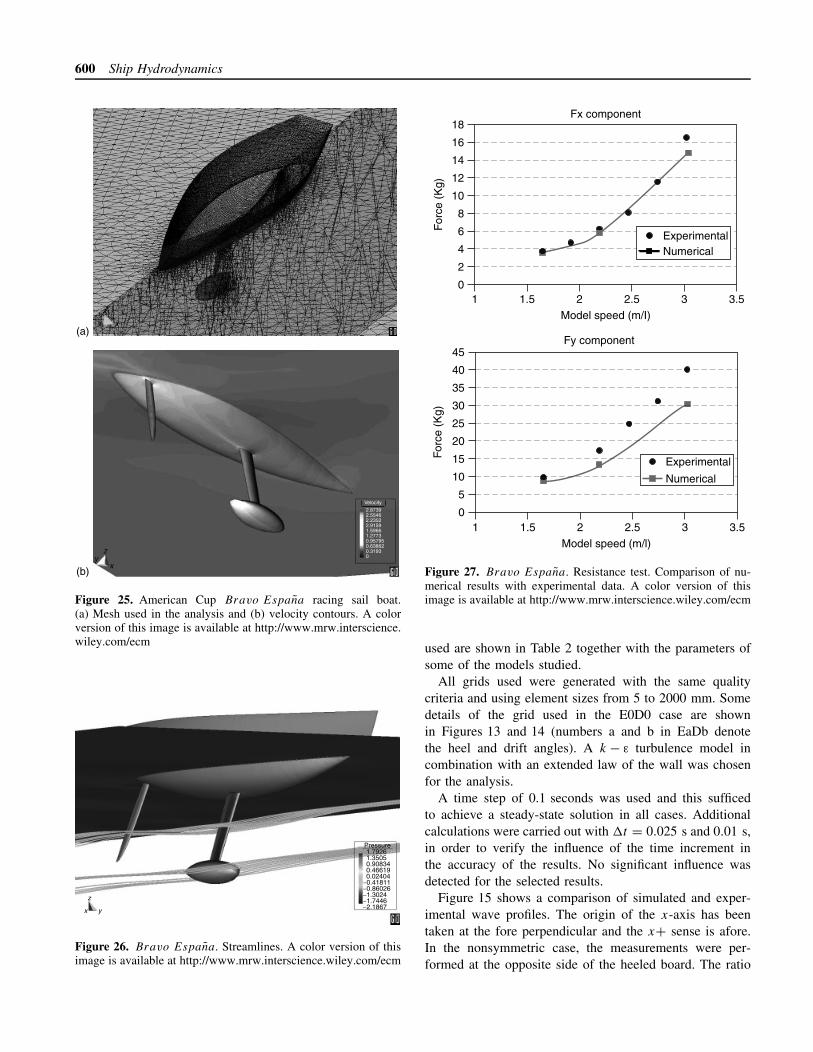
Figure 27. Bravo Espana. Resistance test. Comparison of nu-merical results with experimental data. A color version of thisimage is available at http://www.mrw.interscience.wiley.com/ecm

used are shown in Table 2 together with the parameters ofsome of the models studied.

All grids used were generated with the same qualitycriteria and using element sizes from 5 to 2000 mm. Somedetails of the grid used in the E0D0 case are shownin Figures 13 and 14 (numbers a and b in EaDb denotethe heel and drift angles). A k − ε turbulence model incombination with an extended law of the wall was chosenfor the analysis.

A time step of 0.1 seconds was used and this sufficedto achieve a steady-state solution in all cases. Additionalcalculations were carried out with �t = 0.025 s and 0.01 s,in order to verify the influence of the time increment inthe accuracy of the results. No significant influence wasdetected for the selected results.

Figure 15 shows a comparison of simulated and exper-imental wave profiles. The origin of the x-axis has beentaken at the fore perpendicular and the x+ sense is afore.In the nonsymmetric case, the measurements were per-formed at the opposite side of the heeled board. The ratio


of maximum amplitudes of fluctuations (noise) and wavesin the experimental measurements varies from 4 to 12%.

Figures 16 and 17 show pressure contours on the bulband keel for different cases, corresponding to a velocity of8 kn. Figures 18 and 19 show some of the wave patternsobtained for a velocity of 9 kn. Figures 20, 21, and 22 showsome perspective views, including pressure and velocitycontours, streamlines and cuts for some cases analyzed.Finally, Figures 23 and 24 show resistance graphs wherenumerical results are compared with values extrapolatedfrom experimental data. For further details, see Garcıa et al.(2002).

14.5 American Cup BRAVO ESPANA model

The finite element formulation presented was also appliedto study the racing sailboat Bravo Espana participatingin the 1999 edition of the American Cup. The mesh oflinear tetrahedra used is shown in Figure 25. Results pre-sented in Figures 25–27 correspond to a nonsymmetri-cal case including appendages. Good comparison betweenexperimental data and numerical results was again obtai-ned; further details can be found in Garcıa and Onate(2003).

1.000000e−02 4.100360e−01

9.800030e−01

1.380030e+00

2.060000e+00

2.620010e+00

3.190040e+00

3.710010e+00

6.500000e−01

1.130010e+00

1.680050e+00

2.310040e+00

2.2910010e+00

3.490000e+00

Figure 28. Fixed ship hit by incoming wave.


14.6 Lagrangian flow examples

A number of simple problems have been solved in orderto test the capabilities of the Lagrangian flow formu-lation to solve ship hydrodynamics problem. All exam-ples have been analyzed with the algorithm describedin Section 10. We note again that the regenerationof the mesh has been performed at each timestep.

14.6.1 Rigid ship hit by wave

The first example is a very schematic representation of aship when it is hit by a big wave produced by the collapseof a water recipient (Figure 28). The ship cannot moveand initially, the free surface near the ship is horizontal.Fixed nodes represent the ship as well as the domain walls.The example tests the suitability of the Lagrangian flowformulation to solve water-wall contact situations evenin the presence of curved walls. Note the breaking and

1.000000e−03 9.003200e−02

2.900310e−01

4.900040e−01

6.900050e−01

1.190050e+00

1.490030e+00

1.690000e+00

1.900310e−01

3.900610e−01

5.900370e−01

7.900190e−01

1.2900020e+00

1.600020e+00

Figure 29. Moving ship with fixed velocity.


splashing of the waves under the ship prow and the reboundof the incoming wave. It is also interesting to see thedifferent water-wall contact situations at the internal andexternal ship surfaces and the moving free surface at theback of the ship.

14.6.2 Horizontal motion of a rigid ship in areservoir

In the next example (Figure 29), the same ship of the pre-vious example moves now horizontally at a fixed velocityin a water reservoir. The free surface, which was initiallyhorizontal, takes the correct position at the ship prow andstern. Again, the complex water-wall contact problem isnaturally solved in the curved prow region.

14.6.3 Semisubmerged rotating water mill

The example shown in Figure 30 is the analysis of a rotatingwater mill semisubmerged in water. The blades of themill are treated as a rigid body with an imposed rotatingvelocity, while the water is initially in a stationary flatposition. Fluid-structure interactions with free-surfaces andwater fragmentation are well reproduced in this example.

14.6.4 Floating wood piece

The next example shows an initially stationary recipientwith a floating piece of wood, where a wave is producedon the left side. The wood has been simulated by a liquidof higher viscosity as described in Section 11. The waveintercepts the wood piece producing a breaking wave anddisplacing the floating wood as shown in Figure 31.

14.6.5 Ships hit by an incoming wave

In the example of Figure 32, the motion of a fictitious rigidship hit by an incoming wave is analyzed. The dynamicmotion of the ship is induced by the resultant of the pressureand the viscous forces acting on the ship boundaries. Wenote that the horizontal displacement of the gravity centerof the ship was fixed to zero. In this way, the ship movesonly vertically although it can freely rotate. The positionof the ship boundary at each time step defines a movingboundary condition for the free-surface particles in the fluid.Figure 32 shows instants of the motion of the ship and thesurrounding fluid. It is interesting to see the breaking of awave on the ship prow as well as on the stern when thewave goes back. Note that some water drops slip over theship deck.

1.000000e−03 9.013750e−02 1.900250e−01

4.900070e−01

7.900410e−01

1.090010e+00

3.900090e−01

6.900050e−01

9.900080e−01

2.900520e−01

5.900500e−01

8.900160e−01

Figure 30. Rotating water mill.


t = 0 s(a)

t = 0.29 s

(b)

t = 0.49 s

(c)

t = 0.71 s

(d)

t = 1.23 s

(e)

Figure 31. Floating wood piece hit by a wave.

Figure 33 shows the analysis of a similar problem usingthe same approach. The section of the ship analyzed corre-sponds now to that of a real container ship. Different to theprevious case, the rigid ship is free to move laterally dueto the sea wave forces. The objective of the study was toassess the influence of the stabilizers in the ship roll. Thefigures show clearly how the Lagrangian method predictsthe ship and wave motions in a realistic manner.

14.6.6 Tank-ship hit by a lateral wave

Figure 34 represents a transversal section of a tank-shipand a wave approaching to it. The tank-ship is modeled asa rigid body and it carries a liquid inside, which movesfreely within the ship domain.

Initially (t = 0.00) the ship is released from a fixed posi-tion and the equilibrium configuration found is consistentwith Archimedes principle. During the following time steps,the external wave hits the ship and both the internal and theexternal fluids interact with the ship boundaries. At timest = 6.15 and 8.55 breaking waves and some water drops

Figure 32. Motion of a rigid ship hit by an income wave. Theship is modeled as a rigid solid restrained to move in the verticaldirection.

slipping along the ship deck can be observed. Figure 35shows the pressure pattern at two time steps.

14.6.7 Rigid cube falling in a recipient with water

The last examples show the capacity of the Lagrangianformulation to analyze the motion of solids within water.In the first example, a solid cube is initially free and fallsdown within a water recipient. In this example, the rigidsolid is modeled first as a fictitious fluid with a higherviscosity, similar to the floating solid of Section 14.6.4.The results of this analysis are shown in Figure 36. Notethat the method reproduces very well the interaction of thecube with the free surface as well as the overall sinkingprocess. A small deformation of the cube is produced. Thiscan be reduced by increasing further the fictitious viscosityof the cube particles.

The same problem is analyzed again considering nowthe cube as a rigid solid subjected to pressure and viscousforces acting in its boundaries. The resultant of the fluidforces and the weight of the cube are applied to the centerof the cube. These forces govern the displacement of thecube, which is computed by solving the dynamic equationsof motion as described in the fractional step algorithm of


Time(s): 2.880000

Time(s): 6.240000

Time(s): 8.160000

Time(s): 9.840000

Time(s): 12.000000

Time(s): 16.799999

Figure 33. Ship with stabilizers hit by a lateral wave.

Section 10, similar to the rigid ships of the three previousexamples. Similarly as in those cases, the moving cube con-tours define a boundary condition for the fluid particles ateach time step.

Initially, the solid falls down freely due to the gravityforces (Figure 37). Once in contact with the water surface,the alpha-shape method recognizes the different bound-ary contours, which are shown with a thick line in thefigure. The pressure and viscous forces are evaluated in

Time(s): 0.000000

Time(s): 1.950000

Time(s): 3.000000

Time(s): 4.950000

Time(s): 6.150000

Time(s): 8.550000

Figure 34. Tank-ship carrying an internal liquid hit by wave. Shipand fluids motion at different time steps.

Time(s): 1.950000

Time(s): 6.150000

Figure 35. Tank-ship under lateral wave. Pressure distribution attwo time steps.

the entire domain and, in particular, on the cube con-tours. The fluid forces introduce a negative accelerationin the vertical motion until, once the cube is completely


1.000000e−03

3.700100e−01

6.700100e−01

1.090010e+00 1.120010e+00 1.170010e+00

7.700100e−01 9.000100e−01

4.700100e−01 5.700100e−01

1.700020e−01 2.600100e−01

Figure 36. Solid cube falling into a recipient with water. Thecube is modeled as a very viscous fluid.

Figure 37. Cube falling into a recipient with water. The cubeis modeled as a rigid solid. Motion of the cube and free-surfacepositions at different time steps.

inside the water, the vertical velocity becomes zero. Then,Archimedes forces bring the cube up to the free sur-face. It is interesting to observe that there is a rotationof the cube. The reason is that the center of the floating

Figure 38. Cube falling in a water recipient. The cube is modeledas a rigid solid. The finite element meshes generated at the selectedinstants are shown.

forces is higher in the rotated position than in the initialones.

Figure 38 shows a repetition of the same problem show-ing now all the finite elements in the mesh discretizingthe fluid. We recall that in all the Lagrangian problemsdescribed here, the mesh in the fluid domain is regeneratedat each time step combining linear triangles and quadrilat-eral elements as described in Section 10. Note that somefluid particles separate from the fluid domain. These parti-cles are treated as free boundary points with zero pressureand hence fall down due to gravity.

It is interesting to see that the final position of thecube is different from that of Figure 37. This is due tothe unstable character of the cube motion. A small differ-ence in the numerical computations (for instance, in the


mesh generation process) shifts the movement of the cubetowards the right or the left. Note, however, that a finalrotated equilibrium position is found in both cases.

Further examples of the Lagrangian flow formulation canbe found in Onate, Idelsohn and Del Pin (2003); Onate et al.(2004); and Idelsohn et al. (2002, 2003b).

15 CONCLUDING REMARKS

An overview of different finite element schemes for solvingship hydrodynamics problems has been presented. Thenecessary stabilization in the numerical computation hasbeen provided by the finite calculus formulation of the fluidflow equations accounting for surface-wave effects.

Stabilized finite algorithms for solving a variety of shiphydrodynamics situations using ALE and fully Lagrangiandescriptions have been presented. Both monolithic and frac-tional step algorithms have been derived. The interactionof the motion of the ship structure with the fluid equa-tions can be accounted for in a straightforward mannerwithin the general flow solution schemes. The ALE for-mulation is particularly adequate for ship hydrodynamicsproblems involving free-surface waves of moderate ampli-tude. The Lagrangian flow formulation allows solving in asimple and effective manner, ship hydrodynamics problemsinvolving large motions of the free surface and complexfluid-structure interaction situations.

16 RELATED CHAPTERS

(See also Chapter 2, Chapter 13 of this Volume, Chap-ter 17 of this Volume)

ACKNOWLEDGMENTS

The authors thank Prof. R. Lohner, Prof. P. Bergan, Dr. C.Sacco and Dr. H. Sierra for many useful discussions.

Thanks are also given to Dr. F. Del Pin and Mr. N. Calvofor their help and involvement in solving the problems withthe Lagrangian formulation.

The authors are grateful to Copa America DesafioEspanol SA and CEHIPAR for providing the geometry andexperimental data for the racing boats analyzed and to DetNorske Veritas for providing the geometry of the ship withstabilizers for the analysis shown in Figure 33.

The Spanish company COMPASS Ingenierıa y SistemasSA (www.compassis.com) provided the computer codeTdyn for the numerical simulation of the examples solvedwith the ALE formulation (Tdyn, 2004). This support isgratefully acknowledged.

REFERENCES

Alessandrini B and Delhommeau G. A multigrid velocity-press-ure-free-surface elevation fully coupled solver for calculationof turbulent incompressible flow around a hull. Proceedingsof the 21st Symposium on Naval Hydrodynamics, Trondheim,1996; 40–55.

Alessandrini B and Delhommeau G. A fully coupledNavier–Stokes solver for calculation of turbulent incompress-ible free-surface flow past a ship hull. J. Numer. Methods Fluids1999; 29:125–142.

Aliabadi S and Shujaee S. free-surface flow simulations using par-allel finite element method. Simulation 2001; 76(5):257–262.

Azcueta R, Muzaferija S and Peric M. Computation of breakingbow waves for a very full hull ship. 7th International conferenceon Numerical Ship Hydrodynamics, Nantes, 1999; 6.2.1–6.2.11.

Baba E and Takekuma K. A study on free-surface flow aroundbow of slowly moving full forms. J. Soc. Naval Architects Jpn.1975; 137.

Bai KJ and McCarthy JH (eds). Proceedings of the Workshopon Ship Wave-Resistance Computations, DTNSRDC, Bethesda,1979.

Beck, RF, Cao, Y and Lee T-H. Fully nonlinear water wave com-putations using the desingularized method. Proceedings of the6th International Conference on Numerical Ship Hydrodynam-ics. The University of Iowa: Iowa City, 1993.

Brezzi F, Franca LP, Hughes TJR and Russo A. b = ∫g. Com-

put. Methods Appl. Mech. Eng. 1997; 145:329–339.

Briley WR, Neerarambam SS and Whitfield DL. Multigrid algo-rithm for three-dimensional incompressible high-Reynoldsnumber turbulent flows. AIAA J. 1995; 33(1):2073–2079.

Brooks A and Hughes TJR. Streamline upwind/Petrov-Galerkinformulation for convection dominated flows with particu-lar emphasis on the incompressible Navier–Stokes equations.Comput. Methods Appl. Mech. Eng. 1982; 32:199–259.

Celik I; Rodi W and Hossain MS. Modelling of free-surface prox-imity effects on turbulence. Proceedings of the Refined Mod-elling of Flows, Paris, 1982.

Chiandusi G, Bugeda G and Onate E. A simple method for updateof finite element meshes. Commun. Numer. Methods Eng. 2000;16:1–9.

Chorin AJ. A numerical solution for solving incompressible vis-cous flow problems. J. Comput. Phys. 1967; 2:12–26.

Codina R. A discontinuity-capturing crosswind dissipation for thefinite element solution of the convection-diffusion equation.Comput. Methods Appl. Mech. Eng. 1993; 110:325–342.

Codina R. Comparison of some finite element methods for solvingthe diffusion-convection-reaction equation. Comput. MethodsAppl. Mech. Eng. 1998; 156:185–210.

Codina R. On stabilized finite element methods for linear systemsof convection-diffusion-reaction equation. Comput. MethodsAppl. Mech. Eng. 2000a; 188:61–83.

Codina R. Stabilization of incompressibility and convection thr-ough orthogonal sub-scales in finite element methods. Comput.Methods Appl. Mech. Eng. 2000b; 191:4295–4321.


Codina R. A stabilized finite element method for generalizedstationary incompressible flows. Comput. Methods Appl. Mech.Eng. 2001a; 190:2681–2706.

Codina R. Pressure stability in fractional step finite elementmethods for incompressible flows. J. Comput. Phys. 2001b;170:112–140.

Codina R. Stabilized finite element approximation of transientincompressible flows using orthogonal subscales. Comput.Methods Appl. Mech. Eng. 2002; 191:4295–4321.

Codina R and Blasco J. A finite element formulation for theStokes problem allowing equal velocity–pressure interpolation.Comput. Methods Appl. Mech. Eng. 1997; 143:373–391.

Codina R and Blasco J. Stabilized finite element method forthe transient Navier–Stokes equations based on a pressuregradient operator. Comput. Methods Appl. Mech. Eng. 2000;182:277–301.

Codina R and Zienkiewicz OC. CBS versus GLS stabilization ofthe incompressible Navier–Stokes equations and the role of thetime step as stabilization parameter. Commun. Numer. MethodsEng. 2002; 18(2):99–112.

Codina R, Schafer U and Onate E. Mould filling simulation usingfinite elements. Int. J. Numer. Methods Heat Fluid Flows 1994;4:291–310.

Codina R, Vazquez M, Zienkiewicz OC. A general algorithm forcompressible and incompressible flow – Part III. The semi-implicit form. Int. J. Numer. Methods Fluids 1998; 27:13–32.

Cruchaga MA and Onate E. A finite element formulation forincompressible flow problems using a generalized streamlineoperator. Comput. Methods Appl. Mech. Eng. 1997; 143:49–67.

Cruchaga MA and Onate E. A generalized streamline finite ele-ment approach for the analysis of incompressible flow problemsincluding moving surfaces. Comput. Methods Appl. Mech. Eng.1999; 173:241–255.

Dawson CW. A practical computer method for solving ship-waveproblems. Proceedings of the 2nd International Conference onNumerical Ship Hydrodynamics, Berkeley, 1977; pp. 30–38.

Donea J. A Taylor-Galerkin method for convective transport prob-lems. Int. J. Numer. Methods Eng. 1984; 20:101–119.

Donea J and Huerta A. Finite Element Method for Flow Problems.John Wiley: Chichester, 2003.

Douglas J, Russell TF. Numerical methods for convection dom-inated diffusion problems based on combining the method ofcharacteristics with finite element or finite difference proce-dures. SIAM J. Numer. Anal. 1982; 19:871.

Duncan JH. The breaking and non-breaking wave resistance of atwo-dimensional hydrofoil. J. Fluid Mech. 1983; 126:507–516.

Edelsbrunner H and Mucke EP. Three dimensional alpha-shape.ACM Trans. Graph. 1994; 3:43–72.

Farmer JR, Martinelli L and Jameson A. A fast multigrid methodfor solving incompressible hydrodynamic problems with free-surfaces. AIAA J. 1993; 32(6):1175–1182.

Garcıa J, Onate E, Sierra H, Sacco C and Idelsohn SR. A stabi-lized numerical method for analysis of ship hydrodynamics.In ECCOMAS CFD98, Papaliou K, Tsahalis D, Periaux J andKnorzer D. (eds). John Wiley, 1998; 664–669.

Garcıa J. A Finite Element Method for Analysis of Naval Struc-tures (in Spanish). PhD thesis, Univ. Politecnica de Catalunya,Barcelona, December 1999.

Garcıa J and Onate E. An unstructured finite element solver forship hydrodynamic problems. J. Appl. Mech. 2003; 70:18–26.

Garcıa J, Luco-Salman R, Salas M, Lopez-Rodrı guez M andOnate E. An advanced finite element method for fluid-dynamicanalysis of America’s Cup boat. High Performance YatchDesign Conference, Auckland, 4–6 December, 2002.

Hansboo P and Szepessy A. A velocity-pressure streamlinediffusion finite element method for the incompressibleNavier–Stokes equations. Comput. Methods Appl. Mech. Eng.1990; 84:175–192.

Hino T, Martinelli L and Jameson A. A finite volumen methodwith unstructured grid for free-surface flow. Proceedings of the6th International Conference on Numerical Ship Hydrodynam-ics, Iowa City, 1993 173–194.

Hirsch C. Numerical Computation of Internal and External Flow,Vol. 1. John Wiley: Chichester, 1988; Vol. 2, 1990.

Hirt CW and Nichols BD. Volume of fluid (VOF) method forthe dynamics of free boundaries. J. Comput. Phys. 1981;39:201–225.

Hughes TJR. Multiscale phenomena: Green functions, subgridscale models, bubbles and the origins of stabilized methods.Comput. Methods Appl. Mech. Eng. 1995; 127:387–401.

Hughes TJR and Brooks, AN. A multi-dimensional upwind sc-heme with no crosswind diffusion. Finite Element Methods forConvection Dominated Flows, Hughes TJR (ed.) AMD-Vol. 34.ASME: New York, 1979.

Hughes TJR and Mallet M. A new finite element formulationsfor computational fluid dynamics: III. The generalized stream-line operator for multidimensional advective-diffusive systems.Comput Methods Appl. Mech. Eng. 1986a; 58:305–328.

Hughes TJR and Mallet M. A new finite element formulationsfor computational fluid dynamics: IV. A discontinuity captur-ing operator for multidimensional advective-diffusive system.Comput. Methods Appl. Mech. Eng. 1986b; 58:329–336.

Hughes TJR and Tezduyar, TE. Finite element methods for first-order hyperbolic systems with particular emphasis on the com-pressible Euler equations. Comput. Methods Appl. Mech. Eng.1984; 45:217–284.

Hughes TJR, Franca LP and Hulbert GM. A new finite ele-ment formulation for computational fluid dynamics: VIII. TheGalerkin/least-squares method for advective-diffusive equa-tions. Comput. Methods Appl. Mech. Eng. 1989; 73:173–189.

Idelsohn SR, Calvo N and Onate E. Polyhedrization of an arbi-trary point set. Comput. Methods Appl. Mech. Eng. 2003a;192(22–24):2649–2668.

Idelsohn SR, Onate E and Del Pin F. A Lagrangian meshlessfinite element method applied to fluid-structure interactionproblems. Comput. Struct. 2003b; 81:655–671.

Idelsohn SR, Onate E, Calvo N and Del Pin F. The meshlessfinite element method. Int. J. Numer. Methods Eng. 2003c;58(6):893–912.

Idelsohn SR, Onate E and Sacco C. Finite element solution offree-surface ship-wave problem. Int. J. Numer. Methods Eng.1999; 45:503–508.


Idelsohn SR, Storti M and Nigro N. Stability analysis of mixedfinite element formulation with special mention to stabilizedequal-order interpolations. Int. J. Numer. Methods Fluids 1995;20:1003–1022.

Idelsohn SR, Onate E, Del Pin F and Calvo N. Lagrangian for-mulation: the only way to solve some free-surface fluidmechanics problems. In Fifth World Congress on Computa-tional Mechanics, Viena, 7–12 July, Mang HA, Rammerstor-fer FG and Eberhardsteiner J. (eds). 2002; on CD-ROM, Web:wccm.tuwien.ac.at.

Janson C and Larsson L. A method for the optimization of shiphulls from a resistance point of view. Proceedings of the 21stSymposium on Naval Hydrodynamics, Trondheim, 1996.

Jenson G and Soding H. Ship wave resistance computation. FiniteApprox. Fluid Mech. 1989 II, 25.

Kim YH and Lucas T. Nonlinear ship waves. Proceedings of 18thSymposium on Naval Hydrodynamics, Ann Arbor, 1990.

KRISO (Korea Research Institute of Ships and Ocean Engi-neering). http://www.iihr.uiowa.edu/gothenburg2000/KVLCC/tanker.html.

Larsson L. Proceedings of the 1980 SSPA-ITTC Workshop on ShipBoundary Layers, SSPA Publication No. 90, 1981.

Larsson L, Regnstron B, Broberg L, Li DQ and Janson CE. Fail-ures, fantasies and feats in the theoretical/numerical predictionof ship performance. 22nd Symposium on Naval Hydrodynam-ics, Washington, DC, 10–14 August, 1998.

Lohner R, Morgan K and Zienkiewicz OC. The solution of non-linear hyperbolic equation systems by the finite element me-thod. Int. J. Numer. Methods Fluids 1984; 4:1043.

Lohner R, Yang C and Onate E. Viscous free surface hydrody-namics using unstructured grids. 22nd Symposium on NavalHydrodynamics, Washington, DC, September 1998.

Lohner R, Yang C, Onate E and Idelsohn SR. An unstructuredgrid-based parallel free-surface solver. Appl. Numer. Math.1999; 31:271–293.

Luo H, Baum JD and Lohner R. A finite volume scheme forhydrodynamic free boundary problems on unstructured grids.AIAA-95-0668, 1995.

Miyata H. Time-marching CFD simulation for moving boundaryproblems. Proceedings of the 21st Symposium on Naval Hydro-dynamics, Trondheim, 1996 1–21.

Nakos DE and Sclavounos PD. On steady and unsteady ship wavepatterns. J. Fluid Mech. 1990; 215:256–288.

Newman JN. Linearized wave resistance theory. Int. Seminar onWave Resistance, Tokyo/Osaka; J. Soc. Naval Architects Japan,1976.

Noblesse F and McCarthy JH (eds). Proceedings of the SecondDTNSRDC Workshop on Ship Wave-Resistance Computations,Bethesda, MD, 1983.

Onate E and Idelsohn SR. A mesh free finite point method foradvective-diffusive transport and fluid flow problems. Comput.Mech. 1988; 21:283–292.

Onate E, Garcıa J and Idelsohn SR. Computation of thestabilization parameter for the finite element solution ofadvective-diffusive problems. Int. J. Numer. Meth. Fluids 1997;25:1385–1407.

Onate E, Garcıa J and Idelsohn SR. An alpha-adaptive approachfor stabilized finite element solution of advective-diffusiveproblems with sharp gradients. In New Adv. in Adaptive Com-put. Methods in Mech., Ladeveze P, Oden JT (eds). Elsevier,1998.

Onate E. Derivation of stabilized equations for advective-diffusivetransport and fluid flow problems. Comput. Methods Appl.Mech. Eng. 1998; 151(1–2):233–267.

Onate E. A stabilized finite element method for incompressibleviscous flows using a finite increment calculus formulation.Comput. Methods Appl. Mech. Eng. 2000; 182(1–2):355–370.

Onate E. Possibilities of finite calculus in computational mechan-ics. Int. J. Numer. Meth. Eng. 2004; 60(1):255–281.

Onate E and Garcıa J. A finite element method for fluid-structureinteraction with surface waves using a finite calculus formula-tion. Comput. Methods Appl. Mech. Eng. 2001; 191:635–660.

Onate E and Manzan M. A general procedure for deriving stabi-lized space-time finite element methods for advective-diffusiveproblems. Int. J. Numer. Methods Fluids 1999; 31:203–221.

Onate E and Manzan M. Stabilization techniques for finite ele-ment analysis of convection diffusion problems. In Computa-tional Analysis of Heat Transfer, Comini G, Sunden B (eds).WIT Press: Southampton, 2000, 71–118.

Onate E, Idelsohn SR and Del Pin, F. Fully Lagrangian formula-tion for fluid-structure interaction problems using the finite ele-ment method and finite calculus. In Computational Mechanics –Theory and Practice, Mathisen KM, Kvamsdal T, Okstad KM(eds). CIMNE: Barcelona, 2003.

Onate E, Idelsohn SR, Del Pin F and Aubry R. The particle finiteelement method. An overview. Int. J. Comput. Methods, 2004;1(2).

Onate E, Garcıa J, Bugeda G and Idelsohn SR. A general sta-bilized formulation for incompressible fluid flow using finitecalculus and the finite element method. In Towards a NewFluid Dynamics with its Challenges in Aeronautics, Periaux J,Chamption D, Pironneau O, Thomas Ph (eds). CIMNE: Bar-celona, 2002; 123–160.

Peraire J, Morgan K and Peiro J. The simulation of 3D incom-pressible flows using unstructured grids. In Frontiers of Com-putational Fluid Dynamics, Caughey DA and Hafez MM. (eds),Chapter 16. John Wiley: UK, 1994.

Pironneau O. On the transport-diffusion algorithm and its appli-cations to the Navier–Stokes equations. Numer. Math. 1982;38:309.

Raven H. A Solution Method for the Nonlinear Ship ResistanceProblem. Doctoral thesis, Maritime Research Institute, Delft,1996.

Reed AM, Telste JG, Scragg CA and Liepmann D. Analysis oftranson stern flows. Proceedings of the 17th Symposium onNaval Hydrodynamics, The Hague, 1990.

Sheng C, Taylor LK and Whitfield DL. Implicit lower-upper/app-roximate-factorization schemes for incompressible flows. J.Comput. Phys. 1996; 128(1):32–42.

Soding H. Advances in panel methods. Proceedings of the 21thSymposium on Naval Hydrodynamics, Trondheim, 1996.

Storti M, d’Elia J and Idelsohn SR. Algebraic discrete non-local(DNL) absorbing boundary condition for the ship wave resis-tance problem. J. Comput. Phys. 1998a; 146(2):570–602.


Storti M, d’Elia J and Idelsohn SR. Computing ship waveresistance form wave amplitude with the DNL absorbingboundary condition. Commun. Numer. Methods Eng. 1998b;14:997–1012.

Storti M, Nigro N and Idelsohn SR. Steady state incompressibleflows using explicit schemes with an optimal localpreconditioning. Comput. Methods Appl. Mech. Eng. 1995;124:231–252.

Storti M, Nigro N, Idelsohn SR. equal-order interpolations. Aunified approach to stabilize the incompressible and con-vective effects. Comput. Methods Appl. Mech. Eng. 1997;143:317–331.

Tdyn. A Finite Element Code for Fluid-Dynamic Analysis, COM-PASS Ingenierıa y Sistemas SA, Barcelona, 2004, www.compassis.com.

Tajima M and Yabe T. Simulation on slamming of a vessel byCIP method. J. Phys. Soc. Jpn. 1999; 68:2576–2584.

Tezduyar TE. Stabilized finite element formulations for incom-pressible flow computations. Adv. Appl. Mech. 1991; 28:1–44.

Tezduyar TE. Finite element methods for flow problems withmoving boundaries and interfaces. Arch. Comput. Methods Eng.2001a; 8:83–130.

Tezduyar TE. Adaptive determination of the finite element sta-bilization parameters. Proceeding of the ECCOMAS Computa-tional Fluid Dynamics Conference 2001, Swansea, 2001b.

Tezduyar TE and Hughes, TJR. Finite element formulations forconvection dominated flows with particular emphasis on thecompressible Euler equations. AIAA Paper 83-0125, Proceed-ings of AIAA 21st Aerospace Sciences Metting, Reno, 1983.

Tezduyar TE and Park YJ. Discontinuity capturing finite elementformulations for nonlinear convection-diffusion-reaction prob-lems. Comput. Methods Appl. Mech. Eng. 1986; 59:307–325.

Tezduyar TE, Aliabadi S and Behr M. Parallel finite elementcomputing methods for unsteady flows with interfaces. In

Computational Fluid Dynamics Review 1998, Hafez M,Oshima K (eds). World Scientific, 1998; 643–667.

Tezduyar TE, Behr M and Liou J. A new strategy for finiteelement computations involving moving boundaries and inter-faces – the deforming-spatial-domain/space-time procedure: I.The concept and the preliminary tests. Comput. Methods Appl.Mech. Eng. 1992a; 94:339–351.

Tezduyar TE, Behr M, Mittal S and Johnson AA. Computa-tion of unsteady incompressible flows with the stabilized finiteelement methods. Space-time formulations, iterative strate-gies and massively parallel implementations. In New Methodsin Transient Analysis, AMD-Vol. 143, Smolinki P, Liu WK,Hulbert G and Tamma K (eds). ASME: New York, 1992b7–24.

Tezduyar TE, Mittal S, Ray SE and Shih R. Incompressible flowcomputations with stabilized bilinear and linear equal-orderinterpolation velocity-pressure elements. Comput. MethodsAppl. Mech. Eng. 1992c; 95:221–242.

Wehausen JV. The wave resistance of ships. Adv. Appl. Mech.,1970; 13:93–245.

Wigley. Cooperative Experiment on Wigley Parabolic Modelsin Japan. 17th ITTC Resistance Committee Report, 2nd ed.,1983.

Wilcox DC. Turbulence Modeling for CFD. DCW Industries Inc.:1994.

Xia F. Numerical Calculation of Ship Flows with Special Empha-sis on the Free-Surface Potential Flow. Doctoral thesis, Chal-mers University of Technology, Goteborg, 1986.

Zienkiewicz OC and Codina R. A general algorithm for com-pressible and incompressible flow. Part I: The split charac-teristic based scheme. Int. J. Numer. Methods Fluids 1995;20:869–885.

Zienkiewicz OC and Taylor RC. The Finite Element Method (5thedn), 3 vols. Butterworth-Heinemann, 2000.

chapter 18 ship hydrodynamics - compassis.com€¦ · chapter 18 ship hydrodynamics eugenio onate˜...

Documents