w6 singeqcoint l
DESCRIPTION
Cointegration is an common phenomena in time series data. The material is about some testing procedure for cointegration, namely Augumented Dicky Fuller Test, ARS test.TRANSCRIPT

ECON3350/7350COINTEGRATION
Alicia N. Rambaldi
Week 6
1 / 28

In this lecture
Readings
IntroductionSpurious Regression vs Cointegration
Spurious Regression
CointegrationIntroduction to CointegrationDefinition of CointegrationCointegration OrderExampleTesting for CointegrationProperties of the OLS estimator in the case of cointegration.Testing the cointegration spaceNon-Uniqueness of �
Coming Up
2 / 28
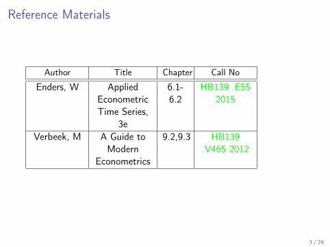
Reference Materials
Author Title Chapter Call No
Enders, W AppliedEconometricTime Series,
3e
6.1-6.2
HB139 .E552015
Verbeek, M A Guide toModern
Econometrics
9.2,9.3 HB139.V465 2012
3 / 28

Spurious Regression vs Cointegration
I What are the implications for empirical economic research ofhaving I(1) variables?
I Spurious Regressions or CointegrationIt is generally true that any combination of two I (1) variableswill also be I (1).
I Spurious RegressionI Conclude there is a significant relationship when there is none.
I CointegrationI Linear combinations of I (1) variables are I (0).
4 / 28

Spurious Regression
I Assume xt
= xt�1
+ ✏x ,t and y
t
= yt�1
+ ✏y ,t where ✏
x ,t and✏y ,t are independent white noise.
I Clearly there is no relationship between xt
and yt
.I If we do not know the above and wish to ’test’ for a
relationship between xt
and yt
, we would normally estimate
yt
= ↵̂+ �̂xt
+ et
I and use a t � test to test
H0 : � = 0 against H1 : � 6= 0
If xt
and yt
were I (0), �̂ would be approximately Normal, twould be approximately Student � t or at leastT
12
⇣�̂ � �
⌘! N(0,V ).
5 / 28

Spurious Regression (cont.)
I But as xt
and yt
are I (1), the distribution of �̂ is moredisperse than Normal and the distribution of t is more dispersethat Student�t.
P(|t| > 1.96) = P(Rejected H0
) > 0.05
I Implications: Tend to reject H0
too oftenI What happens as T ! 1?
I Things get worse and there is no well defined asymptoticdistribution to which �̂ converges:
T12 (�̂ � �) ! 1 and P(|t| > 1.96) increases
6 / 28

Spurious Regression (cont.)
I Indications of a Spurious regression:Signicant t � values; Respectable (sometimes high) R2; lowDurbin-Watson (DW) statistics.
I The signicant t - values occur because the random walks tendto wander, and this wandering looks like a trend.
I If they wander in the same direction for a while (say for thetime of the observed sample), there appears to be arelationship.
I In:I y
t
= ↵+ �xt
+ ✏t
; ✏t
⇠ I (1) so the regression is meaningless.I This explains why DW is low.
7 / 28

Cointegration
I Recall the concept of the stochastic trend
st
= st�1
+ ⌘t
where ⌘t
⇠ I (0)
Any linear combination of st
will be I (1).I Thus if
xt
= ast
+ ⌫x ,t where ⌫
x ,t ⇠ I (0) then xt
⇠ I (1)
8 / 28

Common Stochastic TrendI How can two I (1) variables combine to form an I (0) variable?
I Recall
xt
= ast
+ ⌫x ,t where ⌫
x ,t ⇠ I (0) so xt
⇠ I (1)I Now assume
yt
= st
+ ⌫y ,t where ⌫
y ,t ⇠ I (0) so yt
⇠ I (1)I Then
xt
� ayt
= (ast
+ ⌫x ,t)� a(s
t
+ ⌫y ,t)
= ast
+ ⌫x ,t � as
t
� a⌫y ,t
= ⌫x ,t � a⌫
y ,t which is I (0)
I This is a case of cointegration.I The variables share a common stochastic trend: s
t
.9 / 28

Cointegration and Equilibrium
I The economic interpretation and signicance of cointegrationI We may regard the cointegrating relation
zt
= xt
� ayt
as a stable equilibrium relation.I Although x
t
and yt
are themselves unstable as they are I (1),they are attracted to a stable relationship that exists betweenthem, z
t
⇠ I (0).I For example, there is strong evidence that interest rates are
I (1). But the spread between two rates of different maturities,within the same market, appear to be I (0).
10 / 28

Common Stochastic TrendExample
CWTB3Y: Augmented Dickey-Fuller test statistic -1.253373, p-value (0.6433)
CWTB5Y: Augmented Dickey-Fuller test statistic -1.199108, p-value(0.6673)
SPREAD: Is it I (0)? We return to this question.
The expectations theory of the term structure of interest rateswould suggest that if the interest rates themselves are I (1), thespread between rates of different maturity will be I (0) (Campbelland Shiller,1991).
11 / 28

Definition of Cointegration
I It is possible for a cointegrating relation to involve manyvariables. That is, w
t
may be a (n ⇥ 1) vector. Also wt
maybe integrated of order d .
I A more formal definition of cointegration (Engle & Granger,1987):
Definition
The components of the vector wt
are said to be cointegrated oforder d , b, denoted CI (d , b), if(i) all components of w
t
are I (d),(ii) there exists a vector (� 6= 0) so that
zt
= �0wt
⇠ I (d � b), b > 0
The vector � is called the cointegrating vector.
12 / 28

Cointegration OrderI If w
t
= (w1,t ,w2,t , ...,wn,t)0 ⇠ I (1) but
w 0t
� ⇠ I (0)
I where
�0wt
= w1,t�1 + w2,t�2 + ...wn,t�n
= (�1,�2, ...,�n
)0
0
BBB@
w1,tw2,t
...wn,t
1
CCCA
I Then we say that components of the vector wt
arecointegrated of order 1, 1, denoted CI (1, 1).
I In our simple example above,
wt
=
✓xt
yt
◆and � =
✓1�a
◆
I because xt
� ayt
⇠ I (0).13 / 28

Example
King, R.G., C.I. Plosser, J.H. Stock, and M.W. Watson (1991)."Stochastic trends and economic fluctuations." The American
Economic Review, 81,819-840.
Yt
= �t
K ✓t
L1�✓t
yt
= ln(�t
) + ✓kt
+ (1 � ✓)lt
ln(�t
) = ln(�t�1
) + ✏t
Income = f (Capital , Labour) with technology/productivity shocks�t
14 / 28

Example
(cont.)The economy’s resource constraint implies that output is eitherconsumed or invested, Y
t
= Ct
+ It
, and with common stochastic
trends (�t
) the ratiosCt
Yt
andIt
Yt
(the Great Ratios) are stable.
Therefore, in logs, ct
� yt
and it
� yt
must be I (0) and ct
, yt
, andit
are I (1) but cointegrate.That is
�0wt
=
✓1 0 b
1
0 1 b2
◆0
@ct
it
yt
1
A =
✓ct
+ b1
yt
it
+ b2
yt
◆⇠ I (0)
We also know from the theory that we can restrict b1
= �1 andb2
= �1.
15 / 28

Testing for Cointegration
I Recall that if a vector of I (1) variables do not cointegrate,then no combination of them will be I (0). However, if a vectorof I (1) variables DO cointegrate, then there is a combinationof them that will be I (0).
I Simple solution: to test for cointegration.I Consider the case of three variables: x
t
, yt
, and zt
I Estimate: xt
= ↵̂+ �̂1yt + �̂2zt + et
(by OLS)I Test the residual, e
t
, for a unit root. If et
⇠ I (0), thenxt
, yt
, and zt
cointegrate.
I There are a number of ways we could perform this test. Wewill look at using the Dickey-Fuller test statistic and theDurbin-Watson statistic.
16 / 28

Testing for Cointegration (cont.)
I Because the residual et
comes from a potential cointegratingrelation, the test statistics will not have the usual distributionsso we cannot use the same critical values.
I In both tests we assume et
= ⇢et�1
+ ⌫t
(⌫t
is WN) and testH
0
: ⇢ = 1.I The Augmented Dickey-Fuller test to test for cointegration.
We proceed as usual but use critical values from Table C inEnders.
I The Durbin-Watson test to test for cointegration (CRDW).We proceed as usual but use critical values from Table 9.3 inVerbeek.
17 / 28

Example
Expectations theory of the term structure of interest rates impliesthe following empirically testable feature
If i3y ,t ⇠ I (1) then i
5y ,t ⇠ I (1) and i5y ,t � i
3y ,t ⇠ I (0)
I That is, the long and short interest rates will cointegrateI We had computed:
i3y ,t : Augmented Dickey-Fuller test statistic -1.253373, p-value (0.6433)i5y ,t : Augmented Dickey-Fuller test statistic -1.199108, p-value(0.6673)Thus, they are I (1)
I i5y ,t � i
3y ,t
I H0 : et
= i5y ,t � i3y ,t ⇠ I (1) ,I That is, the long and short interest rates will cointegrate and
we know the cointegrating relation is � = (1,�1).
18 / 28
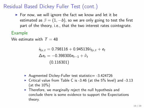
Residual Based Dickey Fuller Test (cont.)I For now, we will ignore the fact we know and let it be
estimated as � = (1,�b), so we are only going to test the firstpart of the theory, i.e., that the two interest rates cointegrate.
Example
We estimate with T = 48
i5y ,t = 0.798116 + 0.945139i
3y ,t + et
�et
= �0.398300et�1
+ ⌫̂t
(0.116301)
I Augmented Dickey-Fuller test statistic= -3.424726I Critical value from Table C is -3.46 (at the 5% level) and -3.13
(at the 10%)I Therefore, we marginally reject the null hypothesis and
conclude there is some evidence to support the Expectationstheory.
19 / 28

Residual Based CRDW
I If the first order autocorrelation is one (⇢ = 1) then theDW ! 0. Thus, the DW of the cointegrating regression goesto zero under the null hypothesis
Example
We estimate with T = 48
i5y ,t = 0.798116 + 0.945139i
3y ,t + et
DW = CRDW = 1.654472
I At the 5% the critical value (Table 9.3 in Verbeek) is 0.72 andthus we reject H
0
: et
⇠ I (1) and conclude there is evidence forthe Expectations theory of the term structure of interest rates.
20 / 28

Properties of the OLS estimator in the case of cointegrationI The OLS estimator �̂ = (↵̂, �̂
1
, �̂2
)0.I In the case of cointegration, the OLS estimator of � will be
superconsistent.I That is, although normal OLS estimates converge to N(0,V )
at the rate T12 , the OLS estimate of a cointegrating vector
converges at the rate T .
I Normally,
⇣�̂ � �
⌘! 0 and T
12
⇣�̂ � �
⌘! N(0,V )
I With cointegration
⇣�̂ � �
⌘! 0 and T
12
⇣�̂ � �
⌘! 0
T⇣�̂ � �
⌘! N(0,V )
21 / 28

Testing the cointegrating space when there is onecointegrating vector
Recall that the Expectations theory of the term structure of interestrates implied
i3y ,t ⇠ I (1) then i
5y ,t ⇠ I (1) and i5y ,t � i
3y ,t ⇠ I (0)
Put another way, if i3y ,t ⇠ I (1) then i
5y ,t ⇠ I (1) because theyshare a common stochastic trend AND the cointegrating vector forthe cointegrating relation is � = (1,�1)0.
I Thus we can test the evidence in support of this theory bysimply calculating z
t
= i5y ,t � i
3y ,t and then testing zt
⇠ I (0)with a simple ADF.
I If we Reject the null hypothesis of a unit root in zt
, then ifi5y ,t ⇠ I (1), then it must hold that i
3y ,t ⇠ I (1) because theyshare a common stochastic trend and the cointegrating vectoris � = (1,�1)0
22 / 28

Testing the more explicit economic theories
Assume wt
=
0
@ct
yt
at
1
Aconsumption
incomewealth (assets)
I If we have a theory that says the cointegrating space is completelyknown, e.g., � = (1,�1,�1)0 say, then we can test the evidence insupport of this theory by constructing the variable z
t
= �0wt
anddoing a test for z
t
⇠ I (1) against zt
⇠ I (0).
Examples
Permanent income hypothesis says
zt
= ct
-yt
= ( 1 �1 )
✓ct
yt
◆⇠ I (0).
I To test this we test for stationarity of zt
(with a simple ADF test).If there is evidence of any form of nonstationarity then this can betaken as evidence against the theory.
23 / 28

The cointegrating space is partially known
I Let the income consumption relation respond to levels ofwealth, e.g., � = (1,�1,�b)0 say, then
I We can test the evidence in support of this theory by
constructing the variable z1,t = (1,�1)0
✓ct
yt
◆= c
t
� yt
and
regressing z1,t on a
t
.
z1,t = µ̂+ b̂a
t
+ et
I Then test for stationarity of et
. If using ADF, useCointegrating ADF statistics with, in this case, two variables.-Table C Enders.
I Note that µ̂ can be interpreted as the mean of the error
correction term zt
.
24 / 28

Non-Uniqueness of �
Recall cointegration with stochastic trend st
where wt
= (xt
, yt
)0
xt
= ast
+ ⌫x ,t where ⌫
x ,t ⇠ I (0) so xt
⇠ I (1) andyt
= st
+ ⌫y ,t where ⌫
y ,t ⇠ I (0) so yt
⇠ I (1)
Then,
�0wt
= (1,�a)0✓
xt
yt
◆
= xt
� ayt
= ⌫x ,t � a⌫
y ,t which is I (0)
Here � = (1,�a)0 because this combination cancelled thestochastic trends.
25 / 28

Non-Uniqueness of � (cont.)
I However,I if 2� = (2,�2a)0 or � = (1,�a)0 for any kappa 6= 0 will also
work as �0wt
⇠ I (0).
�0wt
= (2,�2a)0✓
xt
yt
◆
= 2(xt
� ayt
)
= 2(⌫x ,t � a⌫
y ,t) which is I (0)
I Thus we normalise, � = (1,�a)0 to make � unique.
26 / 28

Example
in the Real Business Cycle model with Balanced Growth Hypthesis(King et al.,1991) we had three variables (c
t
, it
, yt
) and onecommon stochastic trend - productivity shocks.
I Thus, there are n = 3 variables, and n � r = 1 commonstochastic trends. Therefore, r = 2, cointegrating vectors:
� =
2
41 00 1b1
b2
3
5
I Although much emphasis is placed upon estimating thecointegrating vectors, except where r = 1, these vectors arenot interpretable as they are not unique.
I What is unique is the cointegrating space. The cointegratingvectors span (lie in) the cointegrating space.
27 / 28

Coming Up
ARCH, GARCH, Stochastic Volatility and Realised volatility. Testsfor ’ARCH-type’ errors and model identification.
28 / 28