vector functions 13. 13.3 arc length and curvature in this section, we will learn how to find: the...

VECTOR FUNCTIONSVECTOR FUNCTIONS

13

13.3Arc Length

and Curvature

In this section, we will learn how to find:

The arc length of a curve and its curvature.

VECTOR FUNCTIONS

PLANE CURVE LENGTH

In Section 10.2, we defined the length

of a plane curve with parametric equations

x = f(t), y = g(t), a ≤ t ≤ b

as the limit of lengths of inscribed polygons.

[ ] [ ]2 2

2 2

'( ) '( )b

a

b

a

L f t g t dt

dx dydt

dt dt

= +

⎛ ⎞ ⎛ ⎞= +⎜ ⎟ ⎜ ⎟⎝ ⎠ ⎝ ⎠

∫

∫

Formula 1 PLANE CURVE LENGTH

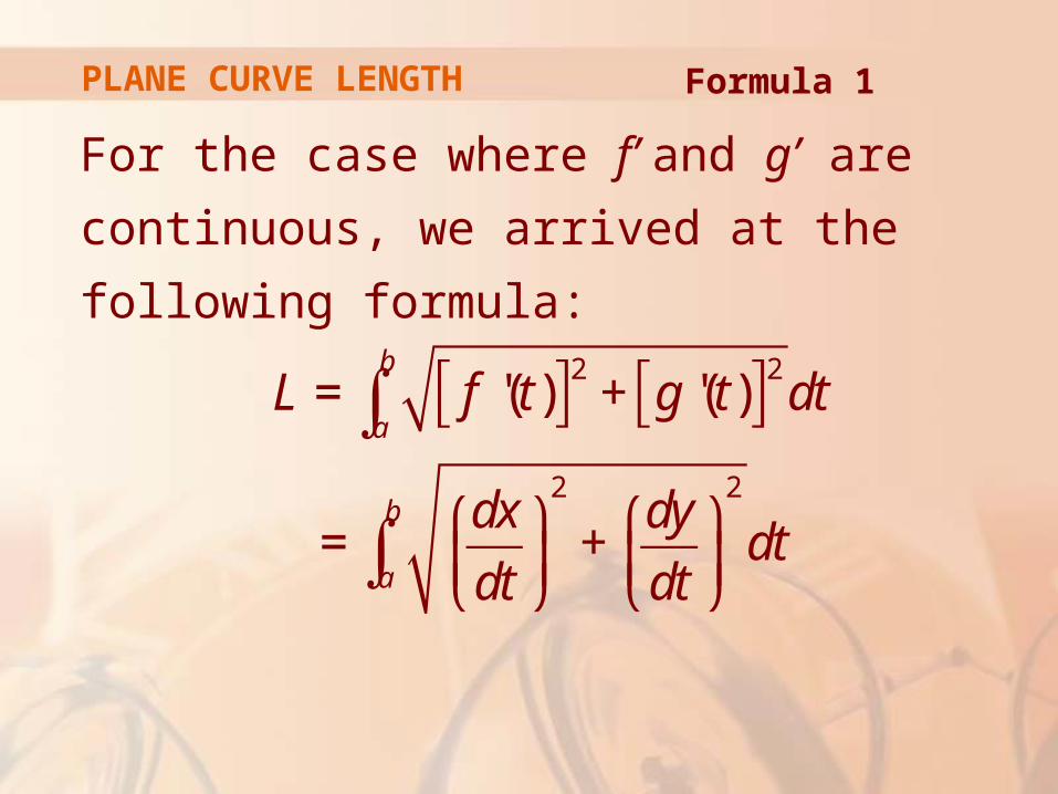
For the case where f’ and g’ are continuous,

we arrived at the following formula:

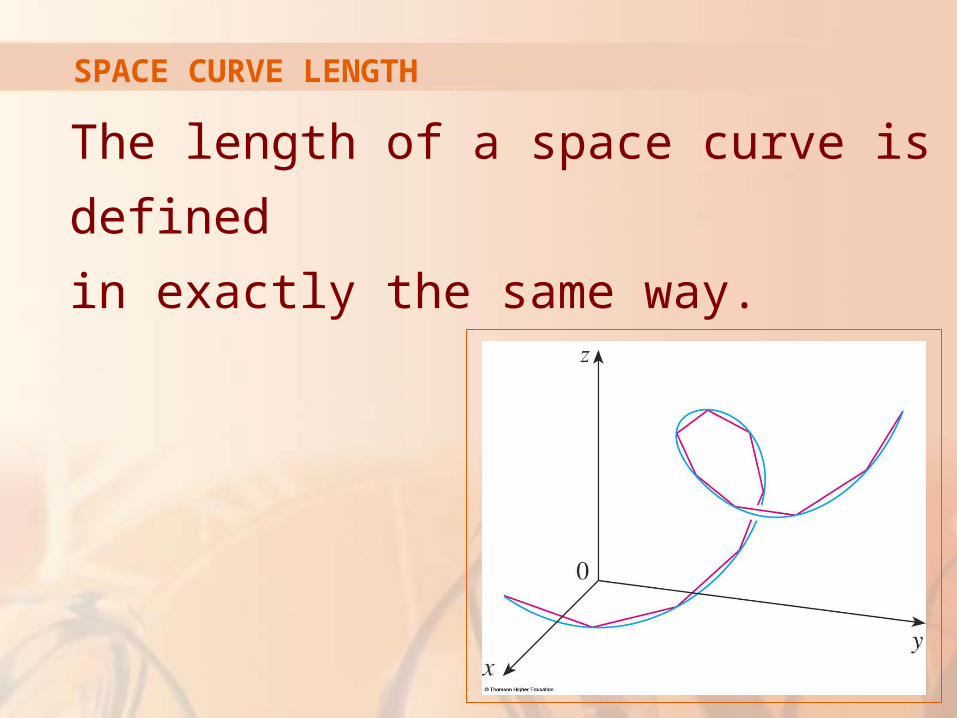
SPACE CURVE LENGTH

The length of a space curve is defined

in exactly the same way.

Suppose that the curve has the vector

equation

r(t) = <f(t), g(t), h(t)>, a ≤ t ≤ b

Equivalently, it could have the parametric equations

x = f(t), y = g(t), z = h(t)

where f’, g’ and h’ are continuous.

SPACE CURVE LENGTH

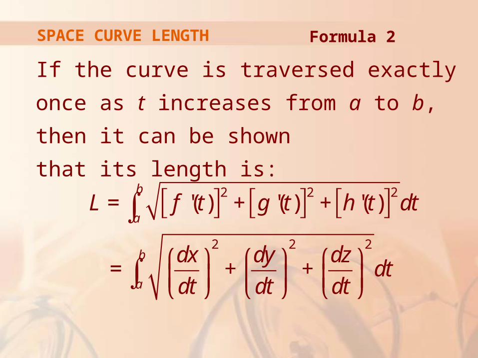
If the curve is traversed exactly once as t

increases from a to b, then it can be shown

that its length is:

[ ] [ ] [ ]2 2 2

2 2 2

'( ) '( ) '( )b

a

b

a

L f t g t h t dt

dx dy dzdt

dt dt dt

= + +

⎛ ⎞ ⎛ ⎞ ⎛ ⎞= + +⎜ ⎟ ⎜ ⎟ ⎜ ⎟⎝ ⎠ ⎝ ⎠ ⎝ ⎠

∫

∫

Formula 2 SPACE CURVE LENGTH

ARC LENGTH

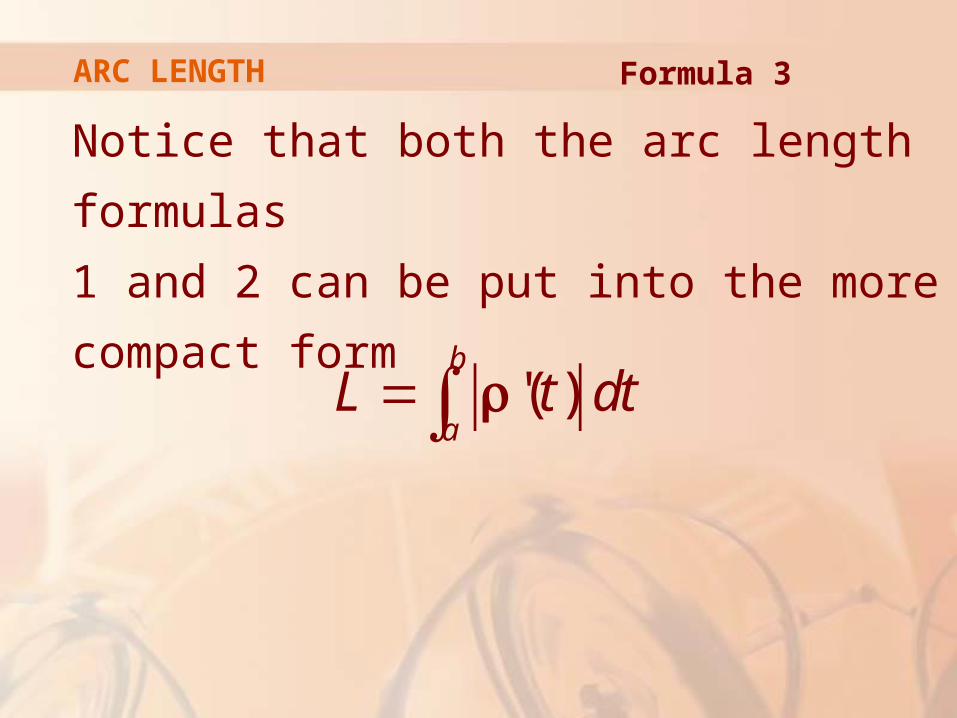
Notice that both the arc length formulas

1 and 2 can be put into the more compact

form

'( )b

aL t dt=∫ r

Formula 3

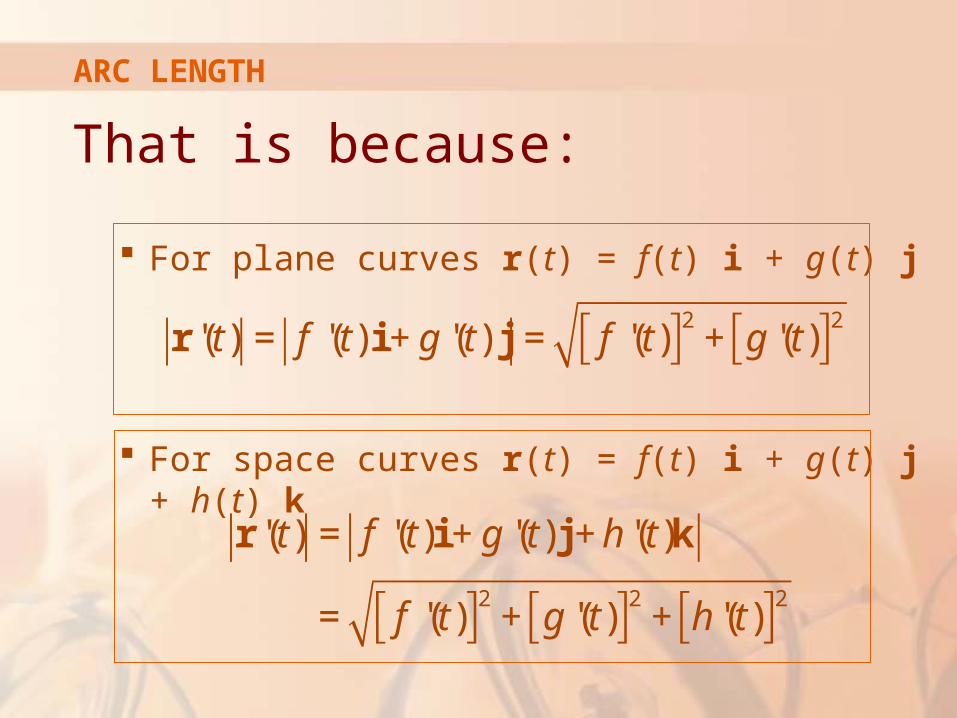
That is because:

For plane curves r(t) = f(t) i + g(t) j

For space curves r(t) = f(t) i + g(t) j + h(t) k

[ ] [ ]2 2'( ) '( ) '( ) '( ) '( )t f t g t f t g t= + = +r i j

ARC LENGTH

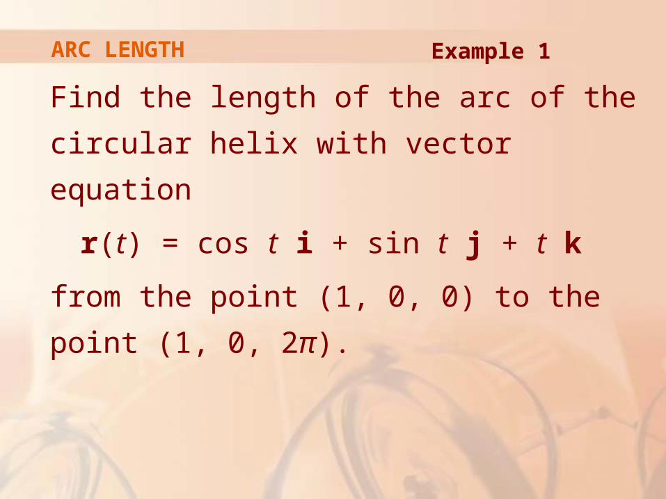
Find the length of the arc of the circular helix

with vector equation

r(t) = cos t i + sin t j + t k

from the point (1, 0, 0) to the point (1, 0, 2π).

Example 1 ARC LENGTH

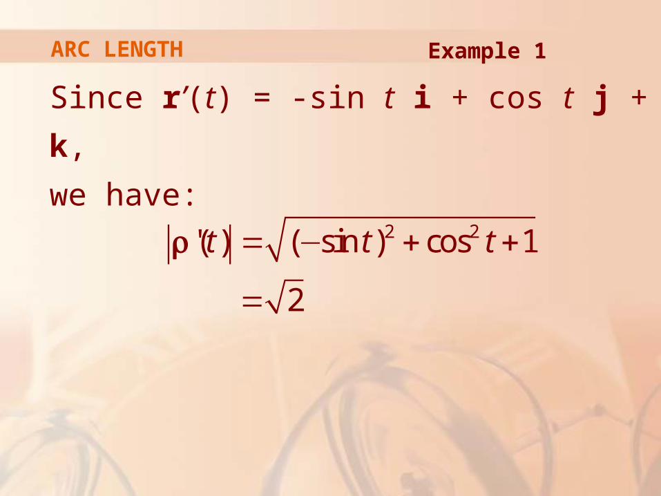
Since r’(t) = -sin t i + cos t j + k,

we have:

2 2'( ) ( sin ) cos 1

2

t t t= − + +

=

r


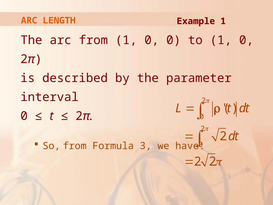
The arc from (1, 0, 0) to (1, 0, 2π)

is described by the parameter interval

0 ≤ t ≤ 2π.

So, from Formula 3, we have:2

0

2

0

'( )

2

2 2

L t dt

dt

π

π

π

=

=

=

∫∫

r


ARC LENGTH

A single curve C can be

represented by more than

one vector function.

For instance, the twisted cubic

r1(t) = <t, t 2, t 3> 1 ≤ t ≤ 2

could also be represented by the function

r2(u) = <eu, e2u, e3u> 0 ≤ u ≤ ln 2

The connection between the parameters t and u is given by t = eu.

Equations 4 & 5 ARC LENGTH

We say that Equations 4 and 5 are

parametrizations of the curve C.

PARAMETRIZATION

If we were to use Equation 3 to compute

the length of C using Equations 4 and 5,

we would get the same answer.

In general, it can be shown that, when Equation 3 is used to compute arc length, the answer is independent of the parametrization that is used.

PARAMETRIZATION

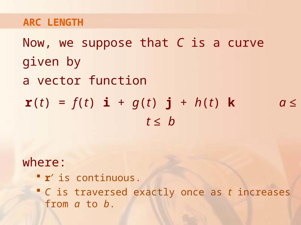
Now, we suppose that C is a curve given by

a vector function

r(t) = f(t) i + g(t) j + h(t) k a ≤ t ≤ b

where: r’ is continuous. C is traversed exactly once as t increases

from a to b.

ARC LENGTH

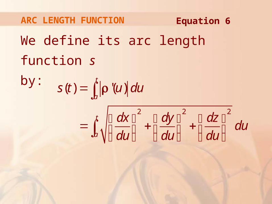
ARC LENGTH FUNCTION

We define its arc length function s

by:

2 2 2

( ) '( )t

a

t

a

s t u du

dx dy dzdu

du du du

=

⎛ ⎞ ⎛ ⎞ ⎛ ⎞= + +⎜ ⎟ ⎜ ⎟ ⎜ ⎟⎝ ⎠ ⎝ ⎠ ⎝ ⎠

∫

∫

r

Equation 6

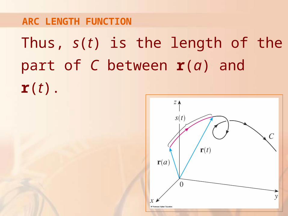
Thus, s(t) is the length of the part of C

between r(a) and r(t).

ARC LENGTH FUNCTION

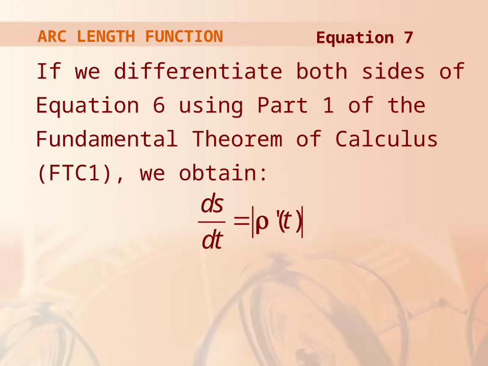
If we differentiate both sides of Equation 6

using Part 1 of the Fundamental Theorem of

Calculus (FTC1), we obtain:

'( )ds

tdt

=r

Equation 7 ARC LENGTH FUNCTION

It is often useful to parametrize a curve

with respect to arc length.

This is because arc length arises naturally from the shape of the curve and does not depend on a particular coordinate system.

PARAMETRIZATION

If a curve r(t) is already given in terms of

a parameter t and s(t) is the arc length

function given by Equation 6, then we may

be able to solve for t as a function of s:

t = t(s)

PARAMETRIZATION

Then, the curve can be reparametrized

in terms of s by substituting for t:

r = r(t(s))

REPARAMETRIZATION

Thus, if s = 3 for instance, r(t(3)) is

the position vector of the point 3 units

of length along the curve from its starting

point.

REPARAMETRIZATION

Reparametrize the helix

r(t) = cos t i + sin t j + t k

with respect to arc length measured from

(1, 0, 0) in the direction of increasing t.

Example 2 REPARAMETRIZATION

The initial point (1, 0, 0) corresponds to

the parameter value t = 0.

From Example 1, we have:

So,

'( ) 2ds

tdt

= =r

0 0( ) '( ) 2 2

t ts s t u du du t= = = =∫ ∫r


Therefore, and the required

reparametrization is obtained by substituting

for t:

/ 2t s=

( ) ( ) ( )( ( ))

cos / 2 sin / 2 / 2

t s

s s s= + +

r

i j k


A parametrization r(t) is called smooth

on an interval I if:

r’ is continuous.

r’(t) ≠ 0 on I.

SMOOTH PARAMETRIZATION

A curve is called smooth if it has

a smooth parametrization.

A smooth curve has no sharp corners or cusps.

When the tangent vector turns, it does so continuously.

SMOOTH CURVE

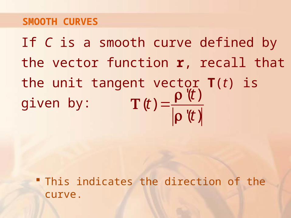
If C is a smooth curve defined by the vector

function r, recall that the unit tangent vector

T(t) is given by:

This indicates the direction of the curve.

'( )( )

'( )

tt

t=r

Tr

SMOOTH CURVES

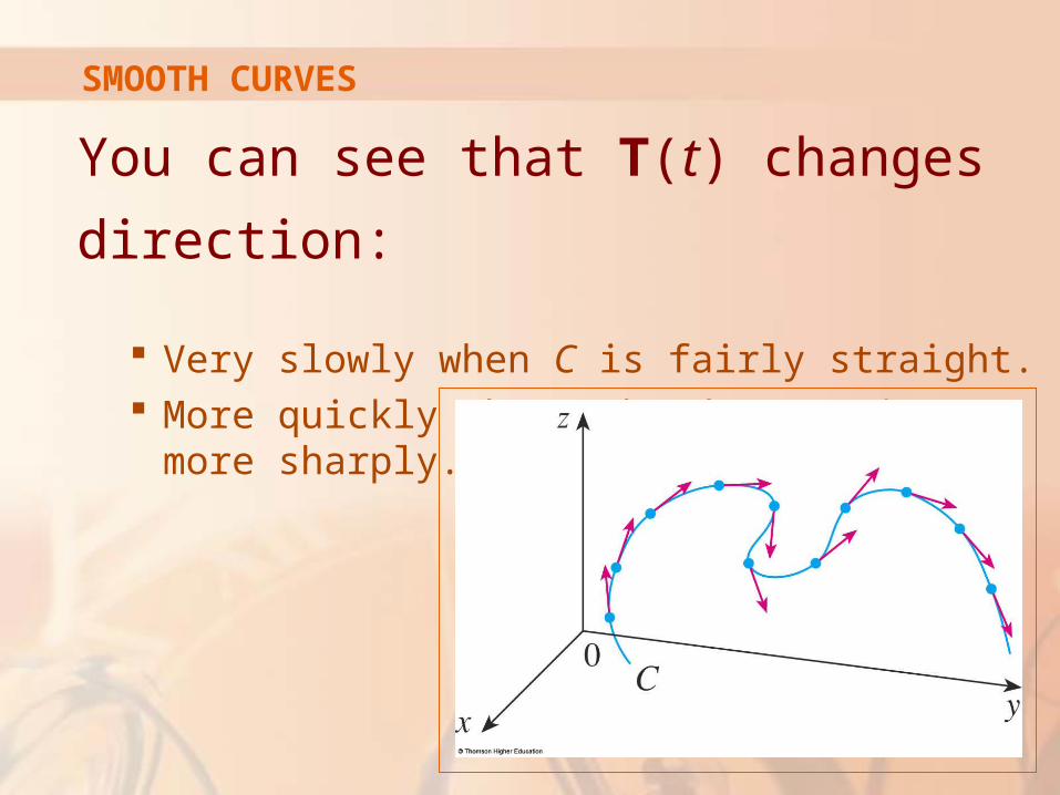
You can see that T(t) changes direction:

Very slowly when C is fairly straight. More quickly when C bends or twists more sharply.

SMOOTH CURVES

The curvature of C at a given point

is a measure of how quickly the curve

changes direction at that point.

CURVATURE

Specifically, we define it to be the magnitude

of the rate of change of the unit tangent vector

with respect to arc length.

We use arc length so that the curvature will be independent of the parametrization.

CURVATURE

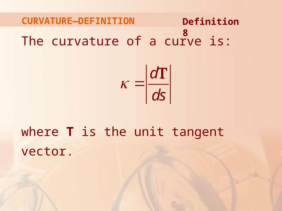
The curvature of a curve is:

where T is the unit tangent vector.

d

dsκ =

T

Definition 8 CURVATURE—DEFINITION

The curvature is easier to compute if

it is expressed in terms of the parameter

t instead of s.

CURVATURE

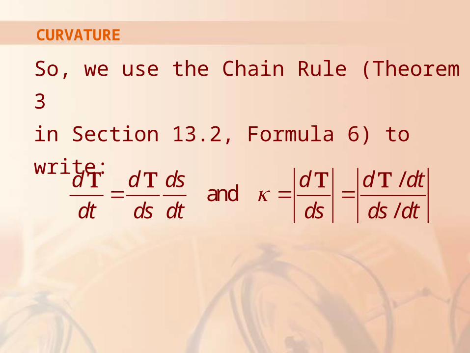
So, we use the Chain Rule (Theorem 3

in Section 13.2, Formula 6) to write:

/and

/

d d ds d d dt

dt ds dt ds ds dtκ= = =

T T T T

CURVATURE

However, ds/dt = |r’(t)| from Equation 7.

So, '( )

( )'( )

tt

tκ =

T

r

Equation/Formula 9 CURVATURE

Show that the curvature of a circle

of radius a is 1/a.

We can take the circle to have center the origin.

Then, a parametrization is:

r(t) = a cos t i + a sin t j

Example 3 CURVATURE

Therefore, r’(t) = –a sin t i + a cos t j

and |r’(t)| = a

So,

and

Example 3 CURVATURE

'( )( ) sin cos

'( )

'( ) cos sin

tt t t

t

t t t

= =− +

=− −

rT i j

r

T i j

This gives |T’(t)| = 1.

So, using Equation 9, we have:

'( ) 1( )

'( )

tt

t aκ = =

T

r

Example 3 CURVATURE

The result of Example 3 shows—in

accordance with our intuition—that:

Small circles have large curvature.

Large circles have small curvature.

CURVATURE

We can see directly from the definition of

curvature that the curvature of a straight line

is always 0—because the tangent vector is

constant.

CURVATURE

Formula 9 can be used in all cases

to compute the curvature.

Nevertheless, the formula given by

the following theorem is often more

convenient to apply.

CURVATURE

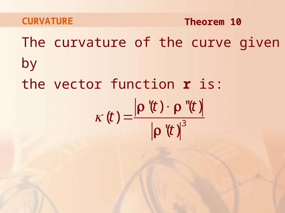
The curvature of the curve given by

the vector function r is:

3

'( ) ''( )( )

'( )

t tt

tκ

×=r r

r

Theorem 10 CURVATURE

T = r’/|r’| and |r’| = ds/dt.

So, we have:

' 'ds

dt= =r r T T

Proof CURVATURE

Hence, the Product Rule (Theorem 3

in Section 13.2, Formula 3) gives:

2

2'' 'd s ds

dt dt= +r T T

Proof CURVATURE

Using the fact that T x T = 0 (Example 2

in Section 12.4), we have:

( )2

' '' 'ds

dt⎛ ⎞× = ×⎜ ⎟⎝ ⎠

r r T T

Proof CURVATURE

Now, |T(t)| = 1 for all t.

So, T and T’ are orthogonal

by Example 4 in Section 13.2

Proof CURVATURE

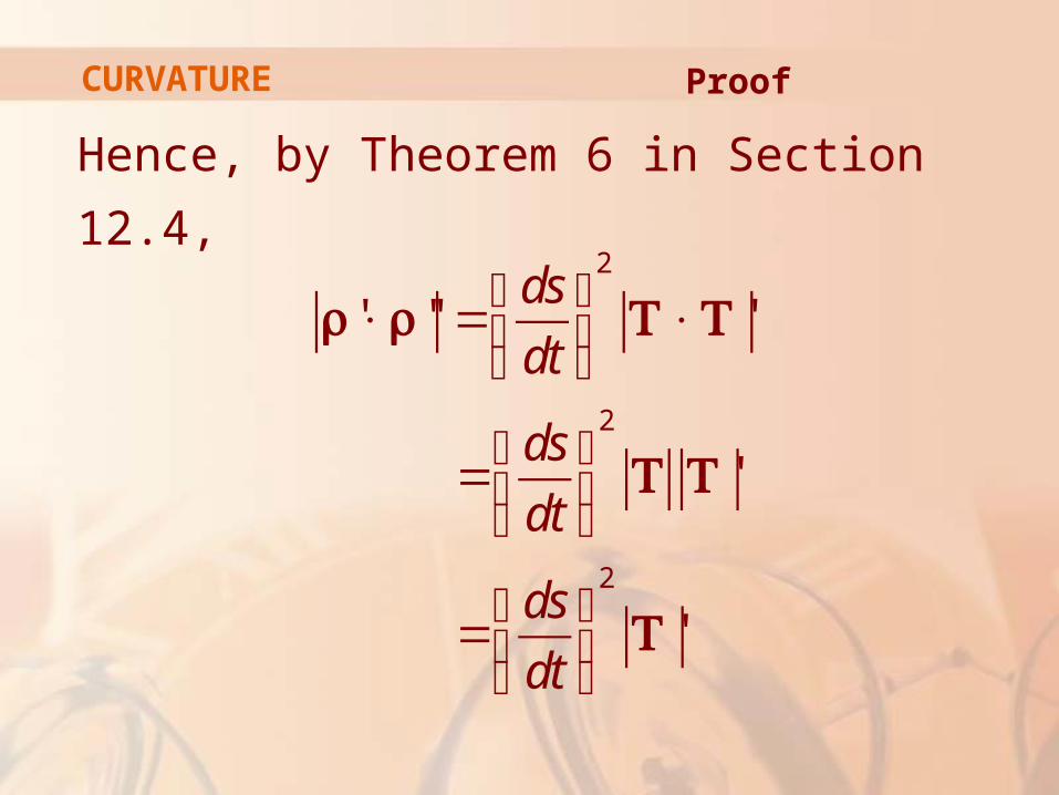
Hence, by Theorem 6 in Section 12.4,

Proof CURVATURE

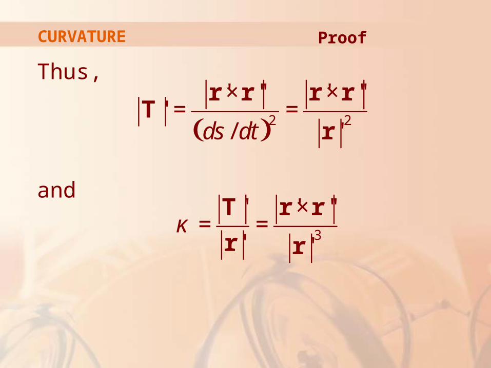
Thus,

and

( )2 2

3

' '' ' '''

/ '

' ' ''

' '

ds dt

κ

× ×= =

×= =

r r r rT

r

T r r

r r

Proof CURVATURE

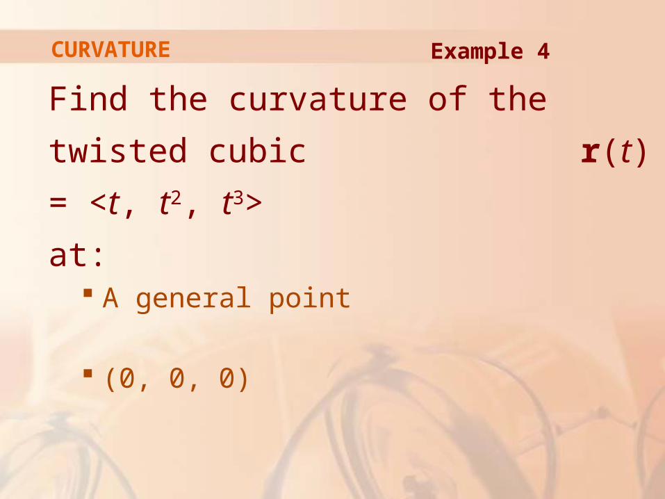
Find the curvature of the twisted cubic

r(t) = <t, t2, t3>

at: A general point

(0, 0, 0)

Example 4 CURVATURE

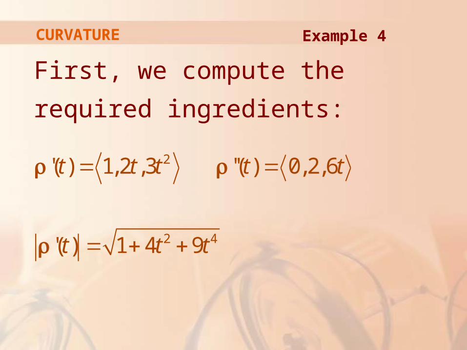
First, we compute the required

ingredients:

Example 4 CURVATURE

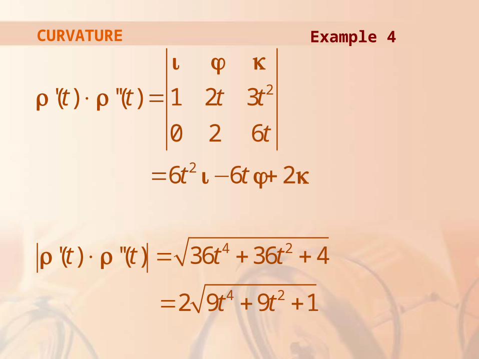
Example 4 CURVATURE

2

2

4 2

4 2

'( ) ''( ) 1 2 3

0 2 6

6 6 2

'( ) ''( ) 36 36 4

2 9 9 1

t t t t

t

t t

t t t t

t t

× =

= − +

× = + +

= + +

i j k

r r

i j k

r r

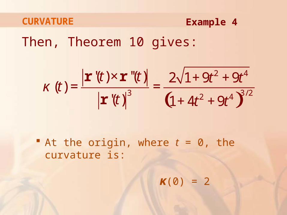
Then, Theorem 10 gives:

At the origin, where t = 0, the curvature is:

ĸ(0) = 2

Example 4 CURVATURE

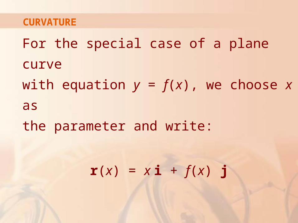
For the special case of a plane curve

with equation y = f(x), we choose x as

the parameter and write:

r(x) = x i + f(x) j

CURVATURE

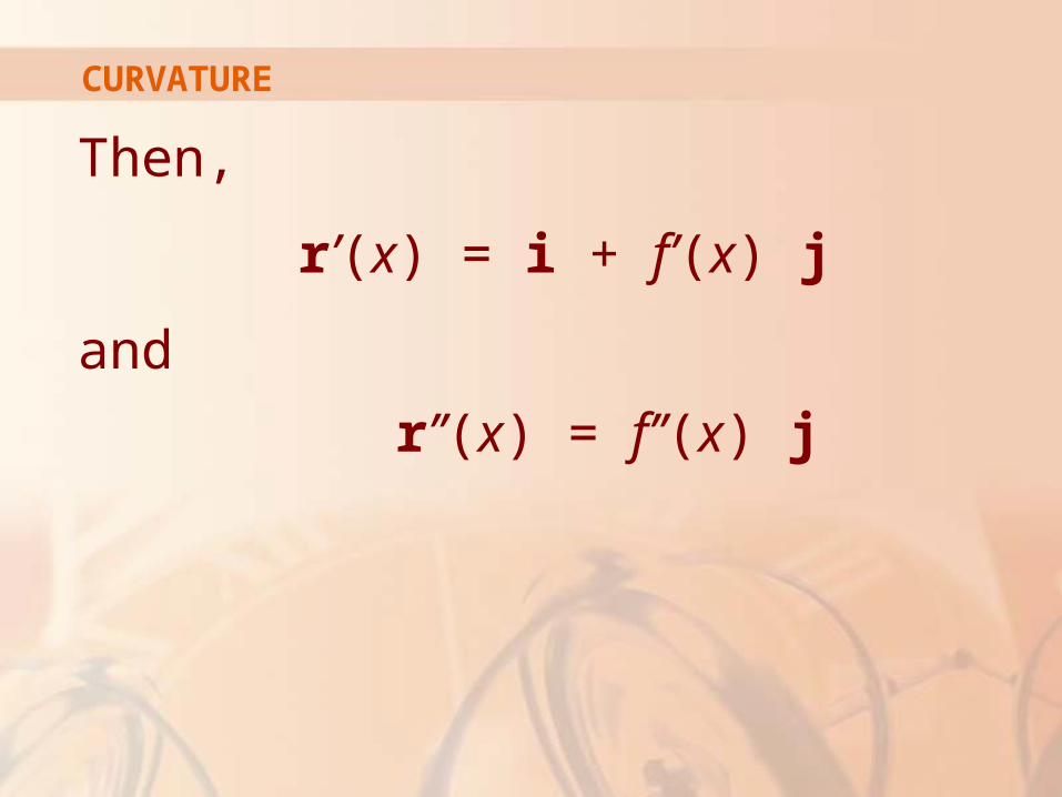
Then,

r’(x) = i + f’(x) j

and

r’’(x) = f’’(x) j

CURVATURE

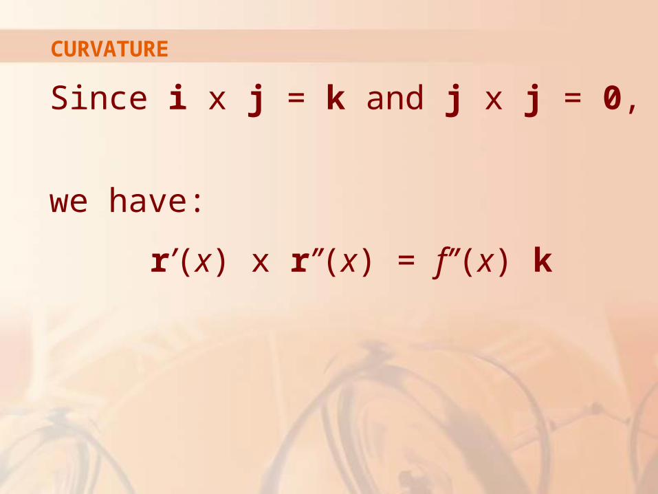
Since i x j = k and j x j = 0,

we have:

r’(x) x r’’(x) = f’’(x) k

CURVATURE

We also have:

[ ]2'( ) 1 '( )x f x= +r

CURVATURE

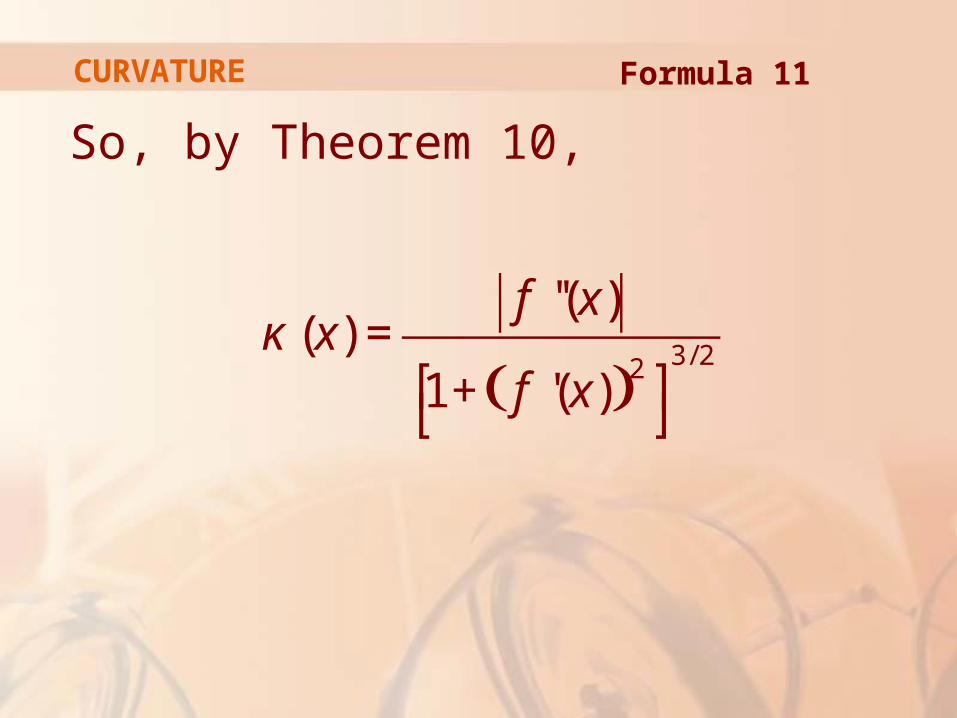
So, by Theorem 10,

( )3/ 22

''( )( )

1 '( )

f xx

f xκ =

⎡ ⎤+⎣ ⎦

Formula 11 CURVATURE

Find the curvature of the parabola y = x2

at the points

(0, 0), (1, 1), (2, 4)

Example 5 CURVATURE

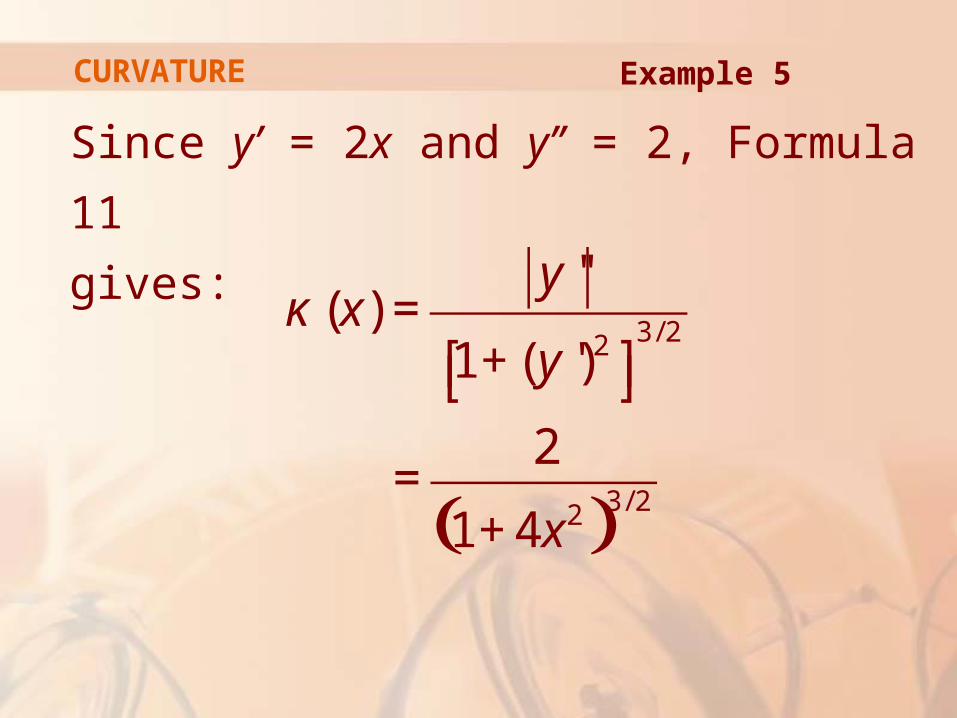
Since y’ = 2x and y’’ = 2, Formula 11

gives:

( )

3/ 22

3/ 22

''( )

1 ( ')

2

1 4

yx

y

x

κ =⎡ ⎤+⎣ ⎦

=+

Example 5 CURVATURE

At (0, 0), the curvature is κ(0) = 2.

At (1, 1), it is κ(1) = 2/53/2 ≈ 0.18

At (2, 4), it is κ(2) = 2/173/2 ≈ 0.03

Example 5 CURVATURE

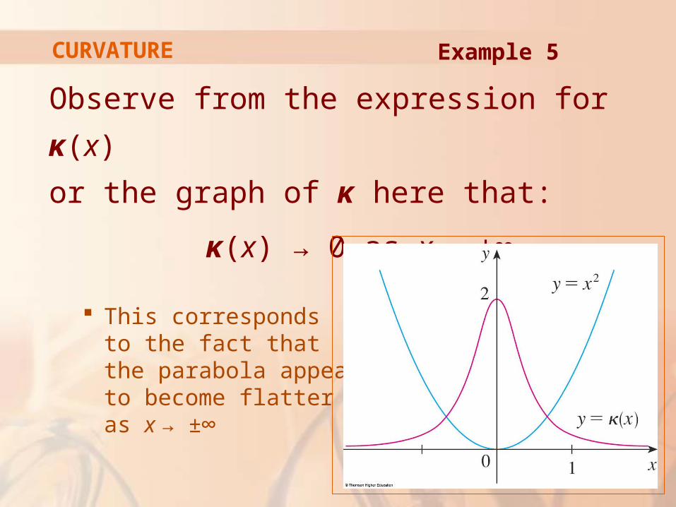
Observe from the expression for κ(x)

or the graph of κ here that:

κ(x) → 0 as x → ±∞

This corresponds to the fact that the parabola appears to become flatter as x → ±∞

Example 5 CURVATURE

NORMAL AND BINORMAL VECTORS

At a given point on a smooth space curve

r(t), there are many vectors that are

orthogonal to the unit tangent vector T(t).

We single out one by observing that,

because |T(t)| = 1 for all t, we have T(t) · T’(t)

by Example 4 in Section 13.2.

So, T’(t) is orthogonal to T(t).

Note that T’(t) is itself not a unit vector.

NORMAL VECTORS

However, if r’ is also smooth, we can

define the principal unit normal vector N(t)

(simply unit normal) as:

'( )( )

'( )

tt

t=T

NT

NORMAL VECTOR

NORMAL VECTORS

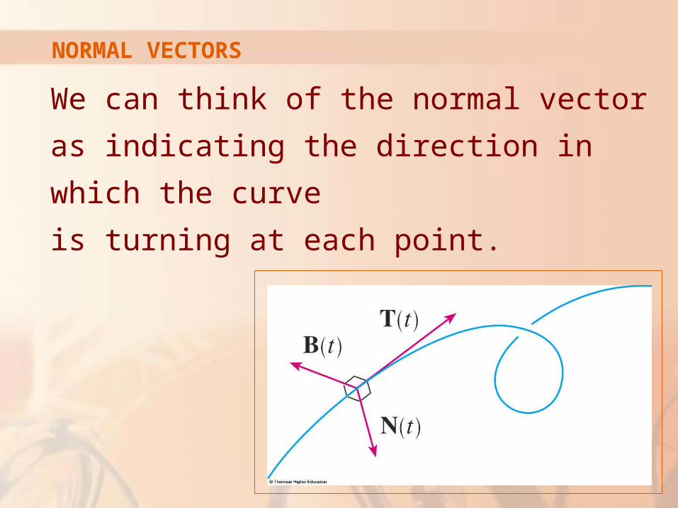
We can think of the normal vector as

indicating the direction in which the curve

is turning at each point.

BINORMAL VECTOR

The vector

B(t) = T(t) x N(t)

is called the binormal vector.

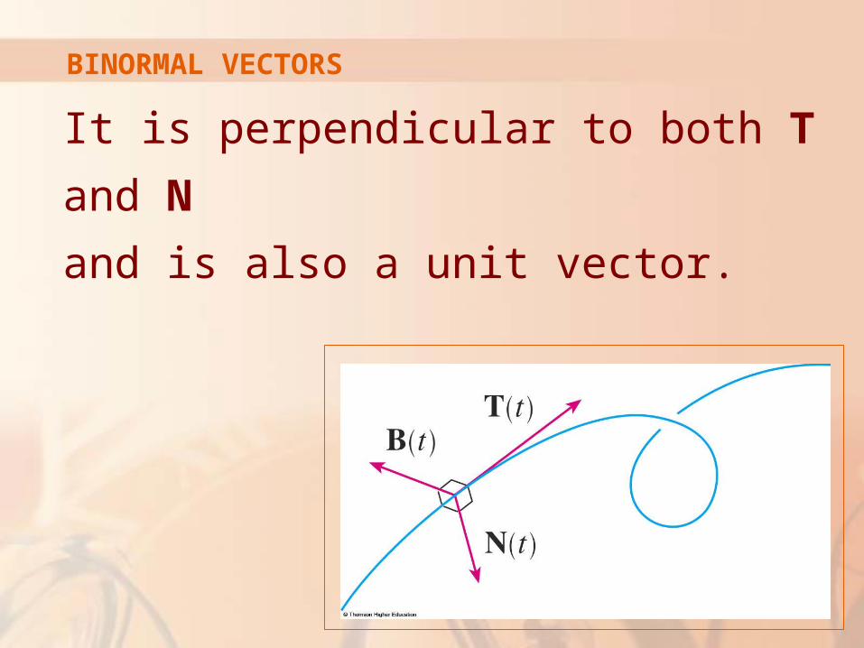
BINORMAL VECTORS

It is perpendicular to both T and N

and is also a unit vector.

NORMAL & BINORMAL VECTORS

Find the unit normal and binormal vectors

for the circular helix

r(t) = cost i + sin t j + t k

Example 6

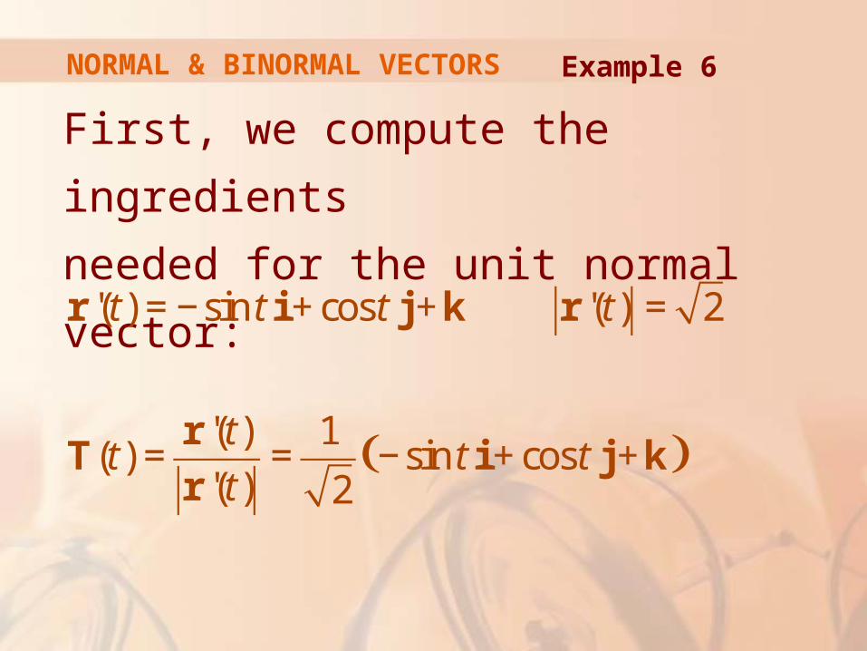
First, we compute the ingredients

needed for the unit normal vector:

( )

'( ) sin cos '( ) 2

'( ) 1( ) sin cos

'( ) 2

t t t t

tt t t

t

= − + + =

= = − + +

r i j k r

rT i j k

r

Example 6 NORMAL & BINORMAL VECTORS

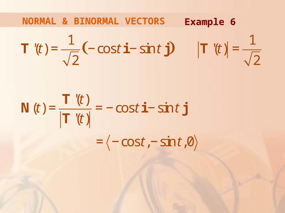
( )1 1'( ) cos sin '( )

2 2

'( )( ) cos sin

'( )

cos , sin ,0

t t t t

tt t t

t

t t

= − − =

= = − −

= − −

T i j T

TN i j

T


This shows that the normal vector

at a point on the helix is horizontal and

points toward the z-axis.


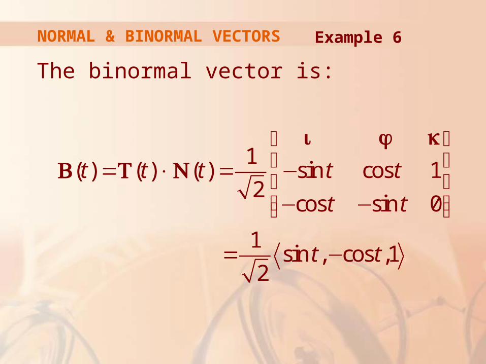
The binormal vector is:

1( ) ( ) ( ) sin cos 1

2cos sin 0

1sin , cos ,1

2

t t t t t

t t

t t

⎡ ⎤⎢ ⎥= × = −⎢ ⎥⎢ ⎥− −⎣ ⎦

= −

i j k

B T N


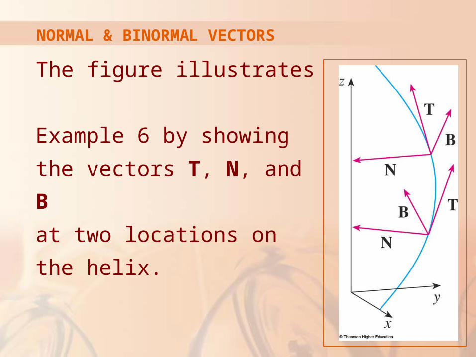
The figure illustrates

Example 6 by showing

the vectors T, N, and B

at two locations on the helix.

NORMAL & BINORMAL VECTORS

In general, the vectors T, N, and B, starting

at the various points on a curve, form a set

of orthogonal vectors—called the TNB frame

—that moves along the curve as

t varies.

TNB FRAME

This TNB frame plays an important

role in:

The branch of mathematics known as differential geometry.

Its applications to the motion of spacecraft.

TNB FRAME

NORMAL PLANE

The plane determined by the normal and

binormal vectors N and B at a point P on a

curve C is called the normal plane of C at P.

It consists of all lines that are orthogonal to the tangent vector T.

OSCULATING PLANE

The plane determined by the vectors

T and N is called the osculating plane

of C at P.

The name comes from the Latin osculum, meaning ‘kiss.’

It is the plane that comes closest to

containing the part of the curve near P.

For a plane curve, the osculating plane is simply the plane that contains the curve.

OSCULATING PLANE

OSCULATING CIRCLE

The osculating circle (the circle of

curvature) of C at P is the circle that:

Lies in the osculating plane of C at P.

Has the same tangent as C at P.

Lies on the concave side of C (toward which N points).

Has radius ρ = 1/ĸ (the reciprocal of the curvature).

It is the circle that best describes how

C behaves near P.

It shares the same tangent, normal, and curvature at P.

OSCULATING CIRCLE

NORMAL & OSCULATING PLANES

Find the equations of the normal

plane and osculating plane of the helix

in Example 6 at the point

P(0, 1, π/2)

Example 7

The normal plane at P has normal

vector r’(π/2) = <–1, 0, 1>.

So, an equation is:

or

( ) ( )1 0 0 1 1 02

2

x y z

z x

π

π

⎛ ⎞− − + − + − =⎜ ⎟⎝ ⎠

= +

Example 7 NORMAL & OSCULATING PLANES

The osculating plane at P contains

the vectors T and N.

So, its normal vector is:

T x N = B


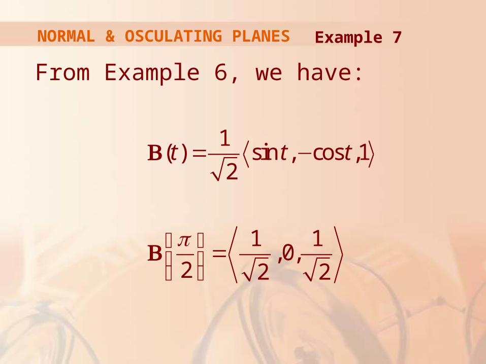
From Example 6, we have:

1( ) sin , cos ,1

2

1 1,0,

2 2 2

t t t

π

= −

⎛ ⎞=⎜ ⎟⎝ ⎠

B

B


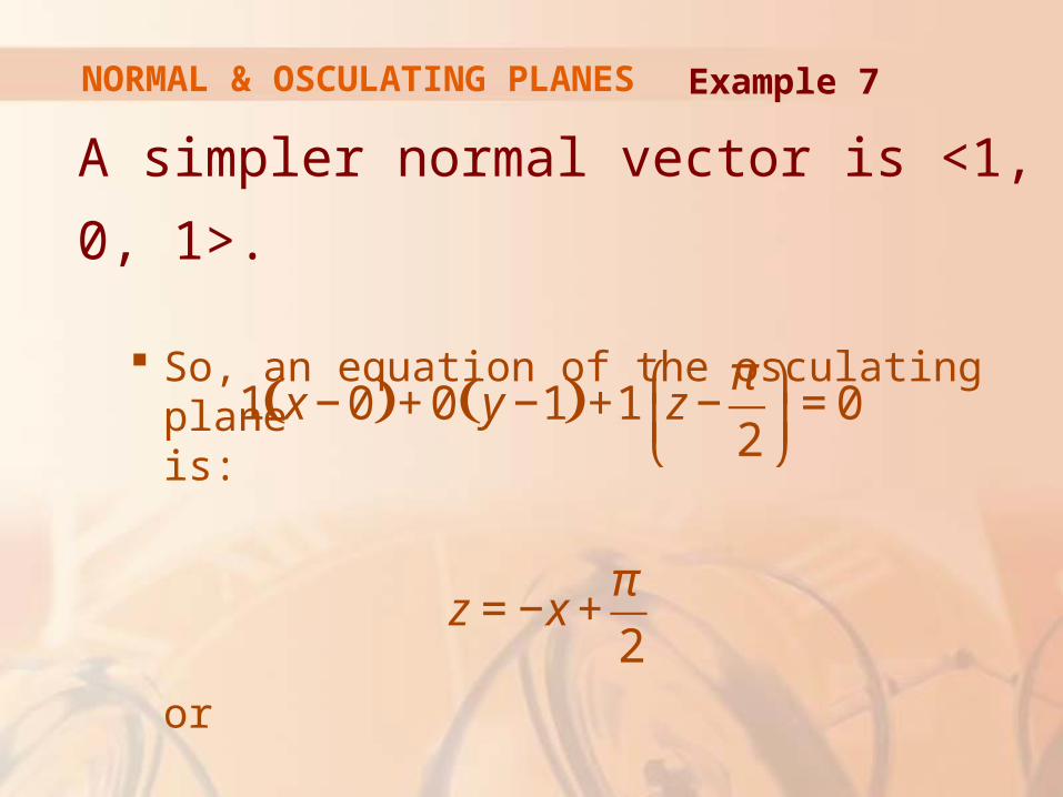
A simpler normal vector is <1, 0, 1>.

So, an equation of the osculating plane is:

or

( ) ( )1 0 0 1 1 02

2

x y z

z x

π

π

⎛ ⎞− + − + − =⎜ ⎟⎝ ⎠

= − +


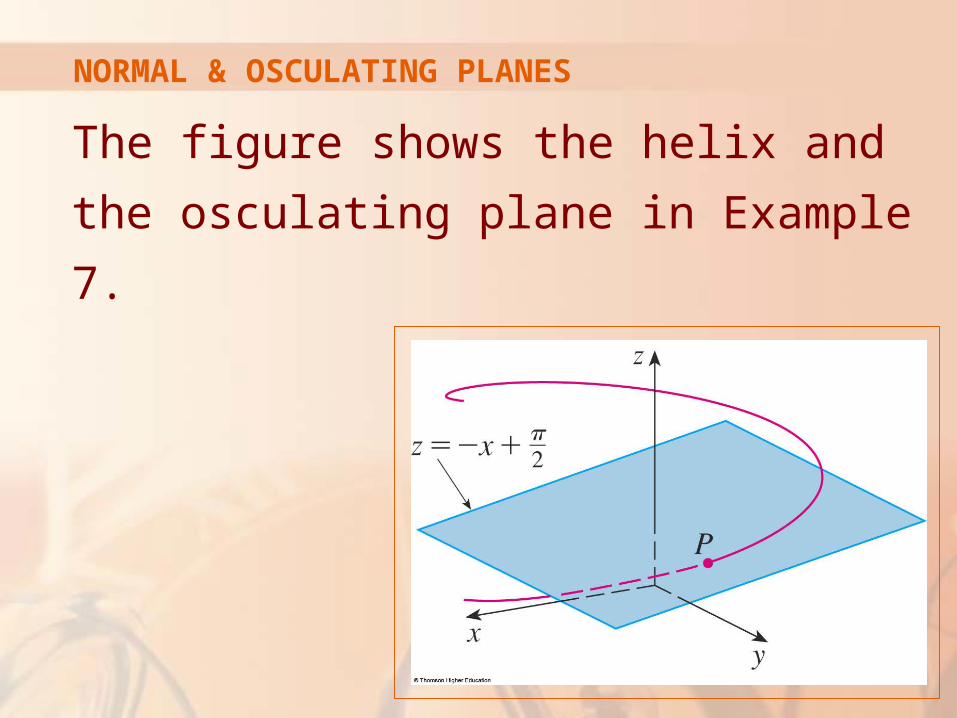
The figure shows the helix and

the osculating plane in Example 7.

NORMAL & OSCULATING PLANES

OSCULATING CIRCLES

Find and graph the osculating circle

of the parabola y = x2 at the origin.

From Example 5, the curvature of the parabola at the origin is ĸ(0) = 2.

So, the radius of the osculating circle at the origin is 1/ĸ = ½ and its center is (0, ½).

Example 8

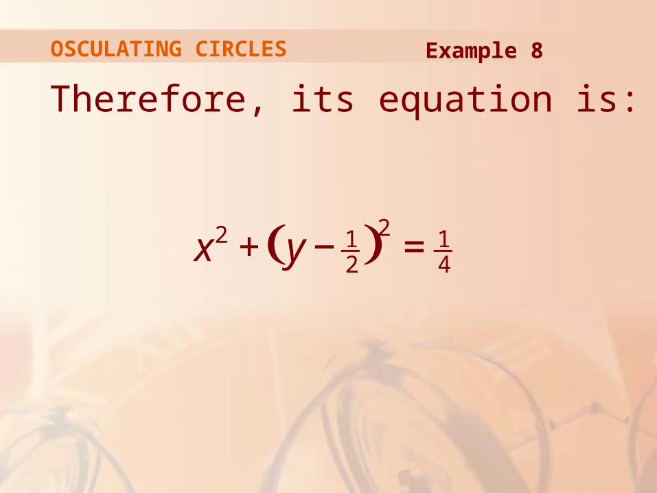
Therefore, its equation is:

( )22 1 12 4x y+ − =

Example 8 OSCULATING CIRCLES

For the graph, we use parametric

equations of this circle:

x = ½ cos t y = ½ + ½ sin t


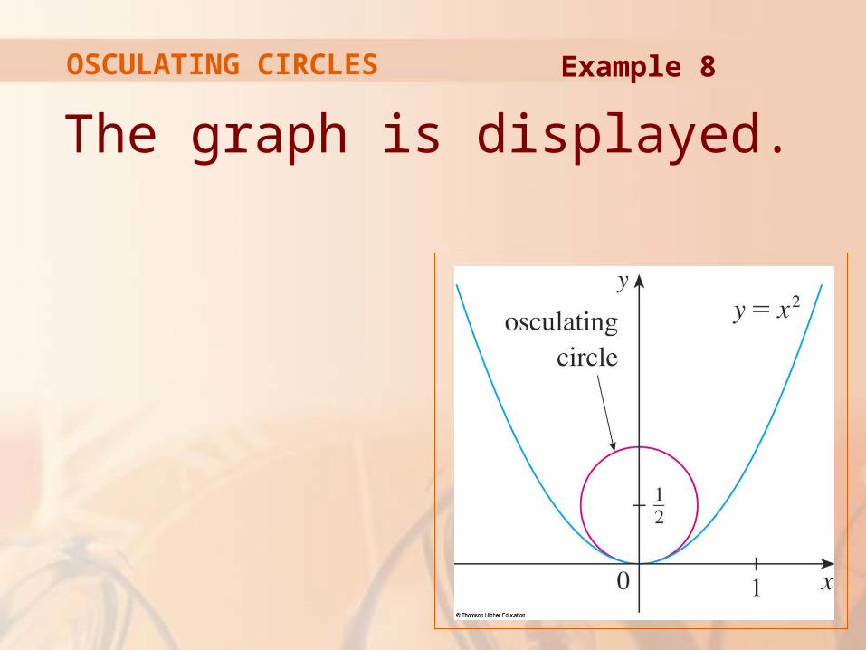
The graph is displayed.


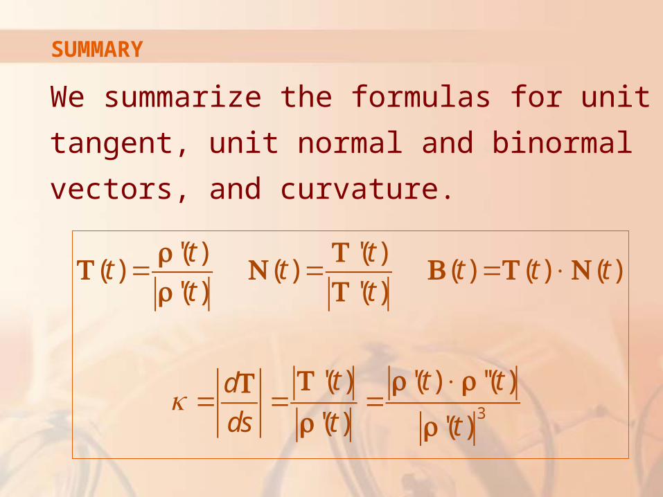
SUMMARY

We summarize the formulas for unit tangent,

unit normal and binormal vectors, and

curvature.

3

'( ) '( )( ) ( ) ( ) ( ) ( )

'( ) '( )

'( ) '( ) ''( )

'( ) '( )

t tt t t t t

t t

t t td

ds t tκ

= = = ×

×= = =

r TT N B T N

r T

T r rTr r

vector functions 13. 13.3 arc length and curvature in this section, we will learn how to find: the...

Documents