Using the Error in Pre-election Polls to Test

for the Presence of Pork

Jacob Allen*

Craig McIntosh**

August 2008

Abstract Polls are used by politicians, voters, and businesspeople alike to form expectations over political outcomes. In an electoral system with ‘pork’ at the national level, local economic prospects will be a direct function of political support. Because every poll comes with its margin of error, we can exploit the error in sub-national polls to test for whether forward-looking investment in the economy adjusts to shocks in local political behavior. The covariance between the strength of this adjustment and local-level characteristics allows us to identify the locations in which strong ‘pork’ contracts exist. To illustrate the technique, we provide a theoretical foundation and an empirical exercise using data on Ugandan micro-entrepreneurs during the 2001 presidential election. We find evidence of transfers which are explicitly conditional on electoral support, and that businesses are most sensitive to surprise voting patterns in ‘core’ districts. Keywords: elections, patronage, pork, polls JEL classification: O16, N27, H42

* PhD Student, International Relations/Pacific Studies, U.C.S.D. jacoballen@ucsd.edu. ** Corresponding Author. Assistant Professor, International Relations/Pacific Studies, U.C. San Diego, 9500 Gilman Drive, La Jolla, CA, 92093-0519. email: ctmcintosh@ucsd.edu, phone: 858 822 1125. Thanks to Gary Cox, and to Stephen Haggard, Gordon Hanson, Ted Miguel, Devra Coren Moehler, Dan Posner, Jeremy Weinstein, participants in seminars at UCSD, UCLA, and APSA, and the staff of FINCA/Uganda; thanks also to Joanitah Kirunda, Robert Apell, Mukalazi Deus, and Jennifer Bartlett for excellent research assistance.

1

1. Introduction.

Politicians have many channels through which they can attempt to engage the electorate in a contract,

offering public largesse in return for support at the ballot box. We refer to any such contract, in which

the flow of public resources is made explicitly conditional on electoral support, as ‘pork’. It is not hard to

motivate why politicians would wish to form such contracts, but establishing the causal link between

political connections and the flow of expenditures has proven more challenging. If, for example, a region

or firm receives high public expenditures as a result of efficiency concerns alone, this should not be

considered pork even if the pattern of expenditures were correlated with political support. Several new

methods have been suggested in recent years to overcome this difficulty and identify the causal chain

through which the fortunes of political actors drive expenditures and therefore changes in investor

behavior. These range from the effect of political prediction markets (Snowberg et al. 2007) to

redistricting (Ansolabehere et al. 2006) to rumors of the ill health of the Indonesian president (Fisman

2001). This paper suggests the error in subnational pre-election polls can be used as a new source of

identification for this relationship.

Specifically, we form the ‘surprise vote share’ as the difference between the final pre-election poll

and the actual outcome of the 2001 Ugandan presidential election at the county level. The single broadly

publicized pre-election poll, conducted by the New Vision newspaper group, give us a straightforward

measure of expected voting patterns prior to the election, and the realization of the outcome of the

election generates a shock to the level of local support for the presidential victor. We then use panel data

on 21,000 microfinance clients to look for evidence of a correlation between this surprise vote share and

abnormal investor borrowing and savings in the immediate aftermath of the 2001 presidential election.

The analysis therefore asks the following question: is investment behavior among microentrepreneurs

responsive to the strength of local political support for the winner of the election? The presence of such a

link would suggest that counties with unexpectedly strong support for the incumbent expect to benefit (or

unexpected opposition counties to suffer) when the favored incumbent wins the election.

2

A large theoretical literature proposes such an exchange between political actors and voters. In

established democracies these exchanges likely take the form of pork-barrel transfers (Cox and

McCubbins 1986, Dixit and Londregan 1996), but personal patronage may be more likely to emerge in

new democracies (Keefer & Vlaicu 2007). We translate the logic of such models into an event study

framework, modeling the process of expectation formation by agents making forward-looking

investments. A natural unit over which expectations of voter behavior are formed is the most

disaggregated unit at which electoral results are widely available, in our case the ‘county’. A simple

model predicts that the localized returns to private investment will be increasing in the scale of political

transfers to local actors (whether through pork-barrel or patronage), and so expected returns are an

increasing function of expected political support. The event which we consider is the difference between

the strength of local support as given by pre-election polls, and actual local support as revealed by the

election. This paper therefore proposes an indirect test for the presence of directly contingent public

expenditures: do shocks to information over local presidential support show up in investor behavior?

There are two steps in the logical chain of this test. First, the equilibrium between politicians and

voters must involve some use of pork or patronage to sway voters. The use of public resources to pursue

political ends in Africa has been widely documented (Miguel & Zaidi 2003, Kasara 2007). Hickey (2003)

writes that Uganda’s primary antipoverty programs ‘have tended to become highly politicized and subject

to both national clientelism and elite capture’. Second, the use of this pork must drive behavior among

the female microentrepreneurs covered by our panel of investment behavior, creating greater ability to

save and invest in the physical areas which received more pork. There has been less research on this

topic, but Hickey (2005) describes the unusual extent to which the Ugandan government has targeted

poverty assistance toward the ‘economically active’, and cross-country evidence exists as to the link

between overall growth and microfinance performance (Ahlin & Lin 2006). Our empirical exercise is

essentially a joint test of both steps in the chain: for the informational shock to drive investment we must

have both a voting-dependent transfer and sensitivity to these transfers among microentrepreneurs.

3

The 2001 Ugandan presidential election provides an interesting application for this test of pork

for several reasons. First, Uganda has a simple majoritarian presidential electoral system, which is more

analytically tractable than an electoral college system. Second, there was only one neutral, widely

publicized poll conducted in the month prior to the election, making it relatively straightforward to

calculate ‘expected’ voting. Third, this race featured a heavy national favorite, incumbent Yoweri

Museveni, squaring off against a rival with strong support in certain regions of the country but never

favored to win the election. For reasons presented in the theory section, the technique outlined in this

paper is most straightforwardly applied to elections without surprises as to the winner of the overall

election. Finally, Uganda’s ‘no-party’ political system combines with the fact that the challenger Kizza

Besigye was from the same region and ethnicity as the incumbent to make the constituencies which

provided electoral support to each candidate rather fluid, and not explicitly ethnic. In this sense, the error

in the polls, revealed on election day, provides a meaningful informational shock.

This paper follows a host of new efforts to attempt to solve the identification problem in

estimating the causal effect of political support on public largesse. A voluminous empirical literature

examines which types of electoral districts receive the most transfers1, but establishing that the

heterogeneity in transfers is driven by political behavior rather than some omitted variable remains a

challenge (Dahlberg and Johansson 2002; Finan 2005; Magaloni, Diaz-Cayeros, and Estévez 2006;

Kasara 2007). Natural experiments such as redistricting (Ansolabehere, Gerber and Snyder 2006) or

national-to-local government party linkages (Arulampalam et al. 2008) provide a useful source of

variation but do not completely resolve the ambiguity over the direction of causality between public

spending and political behavior.2 Hence there has been strong interest in new methods for establishing a

causal link between political support and economic behavior.

1 See, for example, Geddes (1994); Levitt and Snyder (1995); Fleck (1999); Case (2001); Khemani (2003); Miguel and Zaidi (2003); Crampton 2004; Calvo & Murillo (2004); Milligan and Smart (2005); Leigh (2006); Cadot, Röller and Stephan (2006). 2 Indeed, the concept of political business cycles (Drazen 2000) and performance-based incumbent support (Posner and Simon 2002) imply the reverse direction of causality: increases in local economic welfare cause increases in political support.

4

By using an event study methodology to examine the impact of the revelation of new information

on investor behavior, this paper is closest in spirit to work such as Fisman (2001), which uses rumors of

then-president Suharto’s death to test for abnormal returns among Indonesian firms which were closely

connected to his administration. Goldman, Rocholl, and So (2006) show that U.S. firms connected to the

Republican Party had abnormal returns following the 2000 Presidential election, and Jayachandran (2006)

shows that the impact of James Jeffords’ defection to the Democrats on firm values is correlated with the

political contributions that the firm had given to the Republicans.3 Herron (2000) uses Britain’s LIBOR

rates to estimate the counterfactual changes in interest rates and equity markets which would have

obtained had the 1992 British election gone to Labour. A related approach is to use the political

‘connectedness’ of the directors of a firm to test for the probability that a firm gains access to government

procurement contracts (Goldman, Rocholl and So, 2008) or credit from public banks (Khwaja and Mian,

2005).

Political prediction markets provide a new and intriguing metric of political fortunes, attractive

both because we expect such markets to be efficient, and because they vary continuously over time.

Work such as Herron, Lavin, Cram, and Silver (1999) and Snowberg, Wolfers and Zitzewitz (2007) test

for a correlation between movements in prediction markets and the value of specific firms, arguing that

the only reason such a link should exist is that investors perceive the financial fortunes of these firms to

be linked to the outcome of elections. Unfortunately, prediction markets do not exist for Uganda or most

developing countries.

How, then, can we study the links between voting and economic activity in countries with few

publicly traded firms and no prediction markets? The answer provided here to use pre-election polls as

the metric of political expectations, and forward looking investment behavior among microentrepreneurs

as the optimized market outcome. This approach uses the local electoral district as the unit through which

3 A disagreement exists in the empirical literature as to whether political contributions in and of themselves increase future firm value, with Cooper, Gulen, and Ovtchinnikov (2008) finding a positive relationship, whereas Aggarwal, Meschke, and Wang (2008) cast donations as a result of poor corporate governance, and show them to be negatively correlated with future value.

5

politicians and voters interact, and political ‘connectedness’ is given by the degree of expected support for

the eventual winner of the election. The fundamental logic is closely related to other political event

studies in that we suggest there is no reason that investment behavior should be correlated with shocks to

political support unless the investment climate is a direct function of political outcomes.

The strength of the empirical approach outlined in this paper is that it mimics experimental

assignment of political support: because the most likely source for the surprise vote share is the

sampling error in the polls, we have a strong argument that the informational shocks are in fact randomly

assigned. The weakness of the approach is its indirectness, an issue which is related to the question of

what we mean by the use of the term ‘pork’. Most studies of pork analyze specific types of public

expenditure as the dependant variable, and define pork-barrel spending as the provision of localized

public goods in return for electoral support. We infer heterogeneity in the scale of public transfers based

on the behavior of local investors. Our empirical definition of pork is then any form of public

expenditure which is explicitly conditional on local electoral support, and whose use alters the decisions

of local microentrepreneurs. We may equally expect such entrepreneurs to respond to politically driven

public investment (road construction, electrification, telephony) as to clientelistic patronage (bribes and

vote buying putting money in the pockets of local consumers).

We use a model based on Dixit & Londregan (1996) to derive optimality conditions for

politicians’ use of public resources to sway the electorate. In the simplest version of the model, the

politician will push transfers towards each electoral unit until the increase in vote share per dollar

transferred to voters is equalized across units.4 Heterogeneity in the marginal transfer per vote share

arises as a result of ‘leaky bucket’ effects, through which politicians are not equally efficient at

transferring to all constituencies. Aggregate political uncertainty around the time of an election can be

decomposed into a national and a local component. National uncertainty relates to the actual outcome of

the election, while local uncertainty concerns the extent of support for the eventual winner of the election.

4 This constant pork-per-voteshare contract emerges in simple majoritarian systems (where voteshare in each district is equally valuable), while systems with electoral colleges will feature more money transferred for a unit of increased transfers in ‘swing’ districts (where the probability of tipping the majority is highest).

6

In our empirical application, we study the 2001 presidential election in Uganda (a race with a heavy

national favorite) so as to be able to abstract away from the question of who won the election and focus on

the question of the extent to which a region backed the winner. In other words, do local investors expect

that unexpectedly weak local support for a victorious incumbent will prove negative for the local

economic climate? The relationship between the surprise vote share and discontinuous shocks in

investment provide the basis for this test.

To preview our results, we find evidence that investment jumps immediately following the

presidential election in a manner correlated with the size of the surprise support for the victor, Yoweri

Museveni. These effects are statistically significant but not large in magnitude; a 10% surprise increase

in a county’s support for Museveni results in a $1.37 increase in average loan sizes, against an overall

average loan size of $135 and an average residual loan change of $.50.5 This jump in investment is

largest in the counties which form Museveni’s core support, as well as among well-educated, small ethnic

groups. This is consistent with a ‘leaky bucket’ effect in which the efficiency with which the government

can make transfers to groups will determine who the core supporters are. The marginal response to a

positive surprise is larger than the response to a negative surprise.

2. Model.

We begin with a derivation of optimal transfers which is based on a simplification of the theoretical

model of Dixit & Londregan (1996, hereafter D&L).6 They posit a CDF of votes for a particular party

( )i iXΦ , where iX denotes ideological preference for that party. D&L use the index i quite generally

(variously referring to garment workers, ethnic blocs, and states); our application is spatial and so we

define i as the county, the smallest electoral unit at which returns data are available. Transfers can be

5 This change is calculated by regressing loan changes on a set of month and loan cycle fixed effects and taking the average residual. 6 Specifically, we consider only positive political transfers while they consider redistributive taxation and spending; our model therefore considers how best to allocate a strictly positive ‘pork’ budget.

7

used to shift the ‘cut point’ within this distribution, because they increase utility from consumption. iκ

gives the extent to which voters are willing to change their behavior in response to transfers, and we

follow D&L in writing voter utility as 1( ) / (1 )i i iU C C εκ ε−= − , where ε captures the degree of

diminishing marginal returns to private consumption (marginal utility is iCεκ − ). iT is the transfer given

by a politician and i i it Tθ= is the transfer received by the voter; iθ therefore gives the ‘leaky-bucket’

efficiency of the politician at making transfers to a specific electoral unit. As iθ rises towards one it

means that the politician can transfer to a unit with perfect efficiency, and as it goes to zero it means that

the politician is utterly unable to transfer benefits.7 Consumption is given by i i iC Y Tθ= + .

We model a two-party race in which both parties face the same budget constraint B (the ‘spoils of

victory’ define B) and we assume that iκ , the extent to which voters can be bought, is symmetric across

the two parties. Without loss of generality, we consider the decisions of the party that eventually wins the

election, with the ‘opposition’ party denoted by a tilde. Thus the only difference across the two parties is

the transfer efficiency (written as iθ for the winning party and iθ for the opposition party). For an

electoral unit with iN members, equation 12 in D&L establishes the Lagrangian of the constrained

maximization problem as:

(1) 1 1

( ) ( )G G

i i i i ii i

L N X B N Tλ= =

= Φ + −∑ ∑ ,

which has the associated FOC

(2) ( ) ( ) 0 ii i i i i

i

dtN X U C idT

φ λ⎛ ⎞

′ − = ∀⎜ ⎟⎝ ⎠

where iφ is the pdf of the vote share in unit i across received transfers it . 7 This formulation differs from D&L, who separately consider efficiency in taxation and redistribution. We study only the use of positive transfers to buy votes using a fixed pool of resources, rather than the explicit use of taxation as a redistributive game. This model is more analytically tractable than a model of redistributive politics, although the intuition of the first-order conditions is very similar. Also note that D&L define θ as the inefficiency of transfers (meaning a share 1 θ− reaches the electorate), while we define it as the efficiency.

8

Substituting in for the derivative of the utility function, using ii

i

dtdT

θ= , and rearranging terms, (2)

can be written as:

(3) ( ) i i i i iY T iεφ κ θ λ−+ = ∀ .

The term iφ gives the slope of the CDF of the vote share, or the increase in the vote share that is

effected by a marginal increase in received transfers.8 The term ( )i i i iY T εκ θ−+ gives the extent to which

voter behavior is altered by transfers; when iκ is high voters are willing to change their votes in return

for particularistic benefits, and when iθ is high then the politician is effective at getting transfers to the

voters. The number of voters in an electoral unit iN falls out of the maximization because large counties

are symmetrically more important electorally and more expensive to provide a given transfer to each

voter. Hence equation (3) says that the real efficacy of vote share purchased per dollar given must be

equalized across all electoral units in equilibrium.9 The equilibrium transfers for the opposition party are

the same as given by (3), except that iθ is replaced by iθ , the opposition party’s efficiency at making

transfers to unit i.

Equation (3) can be thought of as establishing the terms of a contract between politicians and the

electorate: λ gives the politician’s willingness to pay for incremental vote share in equilibrium. A

additional dollar transferred to voters in an electoral unit will drive up the vote share by a term which is

the product of the willingness of local voters to trade ideology for money ( ( )i i i iY T εκ θ−+ ) and the

8 Our theory abstracts away from the question of the credibility of politicians. A previous version of this paper featured a more complex model which explicitly considered credibility; that formulation generates marginal effects of ‘credibility’ which are observationally equivalent to county-level variation in the slope of φ . Hence in this simpler formulation, we can think of θ as implicitly capturing the credibility channel; if a politician is less credible in a specific county, then promises to that county will result in fewer votes bought and therefore a dampened sensitivity to transfers. 9 Note that the common slope of marginal transfers across units is a product of the assumption in equation (1) of a simple majoritarian election. In a system with an electoral college, marginal vote share in uncontested units has little value to the politician, and transfers focus on those units which are ‘in play’. This means that the slope of the transfer function is steepest when the vote share of the unit is closest to 50%; we propose and execute a test of this proposition in Section 4.4.

9

density of voters at the equilibrium cutpoint ( iφ ). The density of voters at the cutpoint in equilibrium is

( )i

i i i iY T ε

λφκ θ−=

+and the optimal quantity of pork which will go to each county,

1/* i i i

i iT Yεφ κ θ

λ⎛ ⎞= − + ⎜ ⎟⎝ ⎠

. Counties which receive pork are therefore poor, have many swing voters, and

feature efficient transfers to voters who are easily bought.

The pork contract: The left-hand side of (3) is the derivative of vote share iΦ with respect to

transfers iT , which can be written more generally as i

i

ddT

λΦ= . This says that the politician offers a fixed

amount to each electoral unit in return for 1% more support on the margin when the game is in

equilibrium. In order to present a model of optimal transfers which is as transparent as possible, we

consider a linearization of the slope of the pork contract i

i

ddTΦ

around the equilibrium. This linearization

allows us to abstract away from second-order effects, and will provide a reasonable approximation for

local perturbations. Retaining heterogeneity through a unit-specific intercept, we write the vote share as

a function of transfers with the expression i i iTα λΦ = + . The transfers actually received by the voter are

i i it Tθ= , and so this expression can be inverted to give optimal transfers actually received by the voters

as a function of local support;

(4) ( )* 1i i i it α θ

λ= − + Φ .

Optimal transfers from the losing politician would be ( )* 1 (1 )i i i it α θλ

= − + −Φ .

The inverted derivative gives the change in optimal transfers with respect to changes in the vote

share; this can be written as:

(5) *

i i

i

dtd

θλ

=Φ

.

10

Instead of describing how politicians respond to voting, Equation (5) presents the contract from the

perspective of local citizens, giving the money in pocket transferred to them in exchange for support. It

tells us that while the politician will be willing to pay an equal amount for increased vote share anywhere,

that the amount received by voters for a given increase in vote share will be larger the more efficient is

the politician in transferring pork to that constituency.

Political expectations: With this machinery in place, we can specify the way in which pre-

election polls shape expectations of the outcome. The first of these is through P , which gives the ex ante

probability that the eventual winner will win the election. The second is through ip , which gives the

local vote share for the eventual winner, thereby providing an expectation over the strength of regional

support for the winner. If the actual outcome of the vote is i ivΦ = , then the ‘surprise vote share’ can be

defined as i i is v p= − , and the surprise present in the outcome of the election itself is given by 1 P− .

The variance of the surprise vote share is generated by the standard error of the poll itself, whereas the

variance of the national outcome is given by (1 )P P− .10

The ‘surprise’ created by an election can be decomposed into two parts; the resolution of the

uncertainty over the winner of the election (national), and the surprise over the extent to which an

electoral unit backed the winner (local). The expected transfer based on pre-election polls will be

* * *( ( , )) ( ( )) (1 ) ( (1 ))i i i i i iE t P p PE t p P E t p= + − − . Following the linearized from in (4), this can be

written as:

(6) ( ) ( )* 1( ( , )) (1 ) (1 )i i i i i i i iE t P p P p P pα θ α θλ⎡ ⎤= − + + − − + −⎣ ⎦

10 Since the surprise vote share goes to zero as polls become perfectly accurate, we may expect that a ‘poll of polls’ in developed countries which feature many different polls and polling organizations provides less variation off of which to identify this effect. To the extent that all polling houses share sampling mistakes (e.g. turnout patterns themselves were surprising) then elections with multiple polls may provide surprise over local vote shares.

11

The actual transfer made once the outcome of the election is revealed will be *( ) ii i i it v vα θ

λ= − + .

Defining the shock to optimal transfers that arises from the election as * * *( ) ( ( , ))i i i i it t v E t P pΔ ≡ − , we

can then write

(7) * 1 (1 ) (1 )i i i i i i it s P p pθ θ θλ⎡ ⎤⎡ ⎤Δ = + − − −⎣ ⎦⎣ ⎦ .

This equation allows us to decompose the uncertainty in transfers into a national and a local component

by letting is go to zero or P to one, respectively.

As is goes to zero, we remove sampling error from the local poll result and thereby focus on the

surprise caused by the outcome of the election itself. In this case, we see the way in which national-level

political uncertainty enters decision-making:

(7a) * (1 ) (1 )i i i i iPt p pθ θ

λ− ⎡ ⎤Δ = − −⎣ ⎦ .

Because we have defined the outcome of the election as 1P = , the surprise is given by the

quantity 1 P− . Given this, the shifts will be largest where voters are responsive to transfers, and will be

positive if (1 )i i i ip pθ θ> − , This term compares the received transfers from each politician and is

positive if there is heavy support for and efficient transfers from the winner (so the outcome of the

election is a pleasant surprise for locals). If the voters supported the opposition, or could be transferred to

more efficiently by the losing politician, the outcome of the election represents a negative shock to

expected transfers. This term is the product of two questions: “am I surprised?” and “do I care?”. If the

answer to either question is no, then there is no national-level shock to expected transfers from electoral

realizations.

Alternatively, when we eliminate the surprise in national elections by sending P to 1, the

remaining term * i ii

st θλ

Δ = gives the extent to which local pork is driven by the local-level surprise vote

12

share. In other words, when we consider an election in which the outcome itself was not a surprise, the

only uncertainty remaining in an election is the degree of local support for the winner:

(7b) *

0i i

i

d tds

θλ

Δ= > ,

The change in optimal transfers as election results are revealed is now a simple linear function of the

surprise vote share. The slope is steepest where transfers are most efficient, and so (7b) allows us not

only to test for the presence of conditional transfers, but to identify the units for which the bucket leaks

least. This response is based on ‘did we back the winner?’.

The Ugandan case, being an electoral system which had a heavy winner in a simple majoritarian

presidential system, allows us to analyze the case established by equation (7b), where the primary

uncertainty is over the degree of local support. If we were able directly to observe transfers it , we could

use the relationship with the surprise vote share to measure the cross-unit determinants of the term iθ .

We present some aggregated results which suggest that such a reapportionment of explicit budgetary

spending across districts did occur (the simple correlation between the surprise vote share and the change

in district-level budgets before and after the election is .43). However, many forms of political transfers

are intentionally hidden, and so a more interesting empirical test would use an outcome which was

responsive both to formal transfers but also to patronage and explicitly corrupt means for affecting

redistribution.

Investor response to transfers: In order to operationalize the theory, therefore, we propose the

use of forward-looking behaviors which are optimized intertemporally on the basis of expectations, and

which we expect should be sensitive to a broad variety of political transfers. Candidates include business

investment, housing starts, stock prices of local firms with government contracts, and so on. In this paper

we use investment loan decisions taken by the clients of a microfinance lender with offices covering most

of Uganda. We denote this metric by ( )i itπ ; in our application this represents the size of small-business

loans.

13

We abstract away from heterogeneity in this business response by assuming that 'i

i

ddtπ π= is

linear and constant across electoral units, and so investment responds to transfers in a similar way across

electoral units. We can then calculate the responsiveness of local business to the surprise vote share as

the product of business response to transfers and the transfer response to the surprise vote share:

(8) *

* 'i i i i

i i i

d d dtds dt dsπ π θπ

λ= = .

This result can now be taken to the data by measuring the relationship between the discontinuous

jump in investment and the surprise vote share. The significance of the average slope of this relationship

across all electoral units gives us a test for the presence of the use of pork, and variation in the slope

across different units allows us to study which units are most efficiently courted with conditional,

particularistic benefits.

3. Data. Investor data: We measure changes in investor behavior using borrowing records for the clients of

FINCA/Uganda, the country’s largest microfinance lender. These clients are exclusively female,

primarily urban or semi-urban, and typically invest in high-turnover trading businesses. Loans are issued

to groups of roughly 30 borrowers for a 16-week term, and the effective annual rate of interest is over

80%. The lender makes efforts to ensure that this credit is actually being invested in the business, so

changes in borrowing give us an indication of the borrowers’ expected demand in their enterprise over the

four-month period which follows the taking of the loan. We include results for the volume of savings;

however due to the fact that savings in FINCA serve as collateral for loans and the formula for maximum

loan sizes is a repayment grade times the current savings balance, we tend to see savings and investment

co-move.

Are microfinance loans a valid measure for fluctuations in local economic activity? Their

disadvantage is their indirectness; ideally we would prefer a more direct observation on transfers. Our

14

empirical test requires both that voting affects transfers, and that transfers affect average local borrowing.

Extralegal transfers in particular, however, will be hidden from view and therefore not amenable to direct

study. FINCA borrowers are running the bars, small restaurants, groceries, and mobile airtime vendors

who serve the local economy and therefore may be a reasonable place to look for the effects of

expenditures which are hidden. Further, the discontinuity which could be formed on actual spending

would be quite weak (actual expenditures may not adjust immediately). Because we hypothesize that

microentrepreneurs take loans which are increasing in the size of their expected turnover, they incorporate

longer-term expectations into decisions taken days before and days after the election, and therefore may

present a real discontinuity at the time of the election. The independent nature of FINCA’s funding

sources and its centralized infrastructure make it an attractive venue for studying the election. Data

collection is constant across units and time, and it seems unlikely that FINCA had itself become a venue

for distributing pork on the supply side.

The FINCA data is a rolling panel in which each individual features only every four months (or

more) as they ‘recapitalize’ their loans. For this reason, it is difficult to interpret discontinuous changes

between time periods because they consist of different individuals.11 In order to minimize differences

between cohorts we difference outcomes. The dependent variable used throughout the study is

ijt ijt ijπ π π= − for individuals j; the study uses only those individuals who took two or more loans (so as

to avoid entering a zero change for the 11,206 individuals who took only one loan). We thus analyze how

explanatory variables relate to deviations from individual mean outcomes for the 21,140 individuals who

took multiple loans from FINCA during this period. We have accounting data for FINCA clients located

in 71 out of Uganda’s 214 counties, and in 22 out of the 54 districts (these districts represent 56% of the

population of eligible voters in the country). Figure 1 provides a map of the location of all districts in

Uganda and all FINCA groups.

11 The temporal sorting process is non-random, a fact which is easily verified by picking ‘placebo’ discontinuity dates, of which nearly 50% are significant.

15

Voting data: Because we know the district and county in which each borrower is located, we can

take the detailed panel of outcomes provided by FINCA’s institutional data and lay onto it a variety of

information pertaining to political events.12 The first of these is the county-level election results. We use

the percentage of the vote in each county cast for the incumbent Movement candidacy of Yoweri

Museveni, versus the total percentage cast for the opposition candidates combined (Kizza Besigye, along

with Moody Awori, Chapaa Karuhanga, Kibirige Mayanja, and Francis Bwengye).

Polling data: To construct the surprise vote share, we utilize the last neutral opinion poll which

received wide publicity prior to the election. This poll, released by the New Vision on February 28th

2001, got front-page attention in both national English-language papers and in the local-language press.

This poll was designed to be representative at the district level, and was based on 2,994 surveys with a

margin of error of 5%. Results exist for only 19 of Uganda’s 56 districts. FINCA groups exist in 22

districts, of which only 11 overlap with those covered by the opinion polls. From these we have

constructed a county-level prediction of voting based on that found in the district as a whole, or that in the

closest district for which data exist. While this measure is imperfect, it also represents the best

information available to voters in the run-up to the election as to likely voting outcomes; no other polls

existed, and it is not unreasonable to think that voters were using polls to form expectations in a similar

manner. 13

The mean surprise vote share for Museveni was 1.1%, with a large standard deviation of 8.8%.

Whether from large sampling errors in the polls, poor sampling design, or because the polls are at the

district rather than the county level, we have large surprise votes occurring in some locations. While this

12 It is important to note that our use of institutional data in effect weights the impacts we measure by the distribution of FINCA’s clients, and not the distribution of voters in Uganda. Hence we can make no claim that the results we estimate are representative for the average Ugandan voter. 13 We have experimented with two alternative ways of defining the surprise vote share. The first of these is to use either the average of the two pre-election polls or the linear extrapolation based on the difference between them as the measure of ‘expected’ voting. The results are not sensitive to these changes in the manner of predicting the vote. The second is to calculate the vote share only for Museveni and his main opponent in the election, Kizza Besigye, excluding votes for minor candidates. Because the 4 other candidates in the race received less than 2.5% of the votes, the results again are not sensitive to alternate ways of calculating vote shares.

16

implies an imprecise prediction process, it also generates a large amount of variance which can be utilized

in our empirical analysis.

Content Analysis: The 2001 election between incumbent Yoweri Museveni and the upstart

Movement insider Col. Kizza Besigye provides an interesting case study because of the absence of an

explicitly ethnic dimension14 and because it featured an opposition organization built from the ground up

in less than a year. In the absence of entrenched ethnic interests an electoral competition opened up

which was unusually issue-oriented, with a vote for the opposition sending a message of change. The

opposition scored well among the educated, urban, young, and male, and Museveni’s core supporters

were the older rural women with strong memories of the country’s troubled past.

Because we want to avoid confusing the impact of the surprise vote share with other unexpected

events that occurred during the course of the election campaign, we conducted a newspaper content

analysis for the months of November 2000 through July 2001. Uganda has two major newspapers—the

New Vision, owned by the Movement government, and the Monitor, owned by the Aga Khan’s Nation

Media Group. We coded all events of political violence, threats, promises of patronage, and contestation

of election results which could be attributed to a specific time and place. The advantage of having such

data is not only to control for concurrent shocks; comparing the impact of promises of patronage to the

impact of the surprise vote share gives us an interesting check on the direction & magnitude of impact of

the surprise vote share.

We aggregated the events in the content analysis into eight types of political shock:

1. Acts of violence include any attacks, beatings, shootings, etc. which are politically motivated. 2. Threats against the opposition, which includes the following categories from the content analysis:

Government threats to opposition candidates, Government arrests opposing supporters, Government threats to opposing officials, Government supporters threaten opposition, and Physical attack on opposition officials/supporters.

3. Threats against the Movement, includes Opponent supporters threaten government officials, Citizens threaten government, and Physical attack on government official/supporters.

4. Threats against citizens, includes Opponent supporters threaten citizens, Government/police attack/arrest citizens, Citizens struggle with citizens, and Increased security (included because it was an implied threat, and a response to violence).

14 Besigye is from the same ethnic group and region as the incumbent, served as Museveni’s personal doctor during the bush war in the 1980’s, and is married to Museveni’s ex-lover.

17

5. Election results contested. 6. Election was close: This is a dummy which switches on in the month after the election that equals

one if the poll was between 45% and 55%; this variable captures whether the response to the election is a function of local-level uncertainty over the outcome.

7. Movement promise of patronage made to a county by a Movement politician. These include promises of electrification, road construction, or similar statements which can be assigned to a specific location. We refer to these promises as ‘patronage’ to avoid confusing them with the ‘pork’ measured through the primary analysis of the paper.

8. Opposition promise of patronage made to a county by any opposition politician.

Figure 2 illustrates the growing political tension in the months leading up to the March 15th election

date, and the rapid decline after the election; the three months prior to the election saw around 100 events

each, while only 10 occurred in the month afterwards. Table 1 shows the distribution of these events

from the content analysis by district, along with the numbers of FINCA clients in each district. It is clear

from inspection that areas likely to see political events are likely to have FINCA clients. Only Rukungiri

(home to both Museveni and Besigye), Mbale, and Tororo districts saw substantial political activity in the

absence of FINCA clients. Districts in which FINCA clients were present accounted for 74% of the acts

of violence, 73% of threats against opposition, 78% of threats against the Movement, 52% of threats

against citizens, 67% of the Movement patronage promises, and 100% of the opposition patronage

promises.

4. Analysis.

As a first step in our empirical analysis, we perform a simple exercise to verify that a positive

relationship exists between business borrowing and transfers from the government. We calculate the

average jump in microfinance loans at the county level from the two weeks prior to the election to the two

weeks after the election. This jump is then compared to the swing in total funds received by districts from

the central government (as a percentage of total budget) from the fiscal years before and after the election.

While the number of observations here is limited (there are only seven districts for which FINCA data

and budget data exist), the correlation between the jump in loans and the percent change in budgets is .75,

and the correlation between loan changes and the budget share actually received by the district is .83.

18

Figure 3 takes the next step and plots the district-level change in loans against the surprise vote share; the

raw correlation between these two quantities is .39, and the positive relationship is visually clear.

4.1. The mean response to the surprise vote share.

Table 2 gives the basic regression estimates of the impact of the surprise vote share on loan

volume. The first two columns of Table 2 examine a four-month window around the election, using a

variable which is equal to the surprise vote share in the month after the election and zero else. Using this

simple regression we see that the surprise vote share for Museveni displays a positive correlation with

discontinuous increases in borrowing and savings. This implies that the shock of the surprise vote share

induces a meaningful increase in investment at the local level.

The third and fourth columns of Table 2 use data from 14 months around the election (June 2000 –

July 2001, with the election on March 15th 2001), remove time trends with month dummies, and control

for the impact of concurrent political shocks through the events from the content analysis. We use pooled

OLS with standard errors clustered at the district level.15 This regression specification for individual j in

county i at time t is:

8

0 11

ijt t ijt l lit it ijtl

L s uπ β δ β χ β γ=

= + + + + +∑

for the differenced outcome ijtπ . ijtχ is a vector of controls (loan cycle number and cycle squared) that

vary at the individual level over time, and litL is a set of eight dummies equal to one in the month after

new political events are revealed to have occurred in a county. Given the time dummies, these indicator

variables measure how outcomes in counties in the month after each kind of shock has occurred differ

from the average differenced outcomes in that month. its equals the surprise vote share in a county in the

month after the election and zero all other times, so γ measures the extent to which county-specific

changes in economic outcomes in the month after the election are correlated with the surprise vote share.

Because our dependent variables are defined in differences from individual means, the random effects

15 Results are very similar if the regressions are run using county-level instead of district-level clustering.

19

estimator is identical to pooled OLS. The use of fixed effects in this context would only demean the

RHS, and hence the FE estimate is very similar to pooled OLS in all specifications.

Table 2 shows that the surprise vote share has a significant effect on both borrowing and savings

behavior. The implication is that counties which backed Museveni to a surprising extent saw significant

increases in both investment and illiquid savings, indicating an environment which is both better for

investment and more secure. The outcomes are in US Dollars, so the coefficients imply that a 10%

increase in county-level political support leads local investors to invest $1.37 and to save $.50 more in

formal financial institutions.

The impact of the controls from the content analysis are of interest in their own right. Both threats

and promises have measurable effects on borrower behavior. There is some evidence that threats against

the Movement drive up loan sizes, but threats against citizens have a stronger effect; here we see

increased borrowing and sharply decreased savings. This is the only place in the entire analysis in which

savings and loans display divergent responses: the implication is that threats against citizens trigger an

unusual response in which households maximize their short-term liquidity by taking larger loans and

putting less money into FINCA’s relatively illiquid savings product. The response to a patronage promise

is positive, significant, and resembles the effects of the surprise vote share in significance although the

coefficients indicate that the surprise vote share would have to be on the order of 20-40% to rival the

quantity effects of a direct promise of patronage. Intriguingly, the effects of patronage promises by

opposition politicians seem to be larger in both magnitude and significance than those made by the

Movement. It may be that they were more unexpected, causing a bigger discontinuous shift.

There seems to be support here for the idea that changes in business outcomes are related to the

surprise vote share. Figure 4 plots the response to the surprise vote share as we increase the length of the

post-election window used to measure the ‘shock’. Supporting the theory that this informational shock is

both immediate and transitory we see the largest effect using a two-week window and find that by the

time the window has expanded to two months the measured effects become insignificant.

4.2. Is the Surprise Vote Share random?

20

The identifying assumption of the technique presented here is that the surprise vote share comes

from sub-national sampling error in pre-election polls, and therefore should be randomly distributed.

There are several reasons to view the assumption that the error in the polls is random with suspicion. If

the polling firm makes systematic mistakes, or if the ‘surprise’ picks up real last-minute swings in

political preferences, then there may be a direct correlation between the surprise vote and local

characteristics which does not pass through the shock to expectations. We can explore this assumption

due to the fact that if is is indeed a classical error term, the surprise vote will be uncorrelated not only

with pre-election covariates, but with pre-election outcomes as well.

To test this, we use a similar specification to our impact tests, but use the surprise vote share as the

dependent variable in order to test for pre-election orthogonality. We find that pre-election borrowing,

savings, and repayment performance are not related to the surprise vote share, and a wide range of

individual- and county-level characteristics are similarly insignificant (see Table 3). The sole clear

correlation is that education (measured either at the individual level or from district-level data) is strongly

negatively related to the surprise vote share. In other words, educated counties swung more strongly than

expected against Museveni’s Movement government. Whether this correlation arises from random

variation, mis-sampled polling, or arises because of real last-minute changes in political preferences, its

existence moves us from the realm of experimental to quasi-experimental identification.

We can investigate whether education is itself an important contributor to changes in outcomes

by regressing changes in the months prior to the election on education. We accomplish this by interacting

the month dummies for the three months prior to the election with district-level education. In no case are

these interactions significant, and their signs flip from positive to negative. Since education appears to be

having little direct effect on outcomes, the correlation between surprise vote share and education would

not appear to be introducing bias into the causal effect of the surprise vote share on investor outcomes.

4.3. Heterogeneity in the response to surprise vote share.

21

Given this moderate average effect, there are several interesting dimensions across which we can

look at heterogeneity in the responsiveness of local businesses to a given surprise vote share. Equation

(7b) of our theoretical model shows that 'i i

i

ddsπ θπ

λΔ

= ; given the assumption that the business response

to a given shift in transfers is the same across districts, the heterogeneity in the slope of the response to

the surprise vote share is driven by the term iθ . In other words, the response will be strongest in counties

where Museveni is most efficient at delivering transfers.

District level heterogeneity: The empirical study of this response to heterogeneity can be

accomplished through the use of an interaction analysis. For some fixed (and demeaned) district-level

characteristics iZ , we can use OLS to estimate:

8

0 1 21

( * )ijt t ijt l lit i it i it ijtl

L Z s Z s uπ β δ β χ β β γ η=

= + + + + + + +∑ , where η measures the slope of i

i

ddsπ

across iZ . Assuming that the responsiveness of iπ to pork does not differ across counties, the interaction

term η gives us the determinants of iθ : which counties have the buckets that leak least?

Table 4 shows some differentiation of the responsiveness of business to vote share across district-

level characteristics iZ . The districts which show a strong response to the surprise vote share are

educated and rural. This means that educated rural counties have the values of iθ closest to 1, and so

represent a natural core constituency for Museveni.

Ethnic Heterogeneity: Given the (apparently) ethnic nature of many African electoral contests,

another interesting dimension along which to examine variation in slopes in response to surprise vote

share is ethnicity. Using the language spoken in group meetings as a proxy for ethnicity we again find

strong differentiation in slopes, although we have data on language spoken for only 37,635 of our 58,731

observations. Table 5 presents the results of interactions performed in the same way as described above

where we dummy out seven language categories, leaving Kiswahili-speakers as the omitted category.

22

Swahili is the language of trade in East Africa but is not widely spoken in Uganda, and so these groups

are likely to be ethnically heterogeneous and to be trading over larger distances than other groups.

We find that neither English-speaking groups (which may be the most highly educated) nor the major

ethnicities of southern Uganda (the Baganda and Basoga) have slopes which differ from Kiswahili

speakers. However, two kinds of ethnicities have sharply divergent responses. On one hand ethnicities

from the war-torn north of Uganda, where Museveni has struggled to establish authority, show much

lower response to the surprise vote share. On the other hand the four small, non-northern ethnicities show

much larger responses. The implication is that Museveni is more efficient at transferring resources to

small southern ethnic groups than he is to the large groups which dominate southern Uganda. The

complete inability to transfer resources to the North implied by these results is interesting in light of the

long-running civil war being fought by the Movement government against the Lord’s Resistance Army

(LRA) on Northern soil. This conclusion is intuitively appealing and may be driven by the fact that small

ethnic groups can more easily overcome collective action problems in order to provide an efficient

political machine (Olson 1965, Bates 1981).

4.4. Core versus Swing voters.

A major theoretical debate has taken place over whether politicians will target pork to core or

swing constituencies. Cox and McCubbins (1986) assume risk-averse incumbents, concluding that they

will steer transfers disproportionately to their core supporters in order to maintain coalitional stability.

Dixit and Londregan (1996), on the other hand, argue that the incumbent’s core supporters will only

benefit when the incumbent has an organizational advantage in directing favors to the core. Otherwise,

welfare transfers will be directed to voters whose value for material utility is high relative to their

ideological persuasions. By definition these voters are typically swing voters.16 Perhaps not surprisingly

16 Lindbeck and Weibull (1987) reach a similar conclusion. Case (2001), Miguel and Zaidi (2003), Levitt and Snyder (1995), Stokes (2005), and Magaloni, Diaz-Cayeros, and Estévez (2006) find evidence supporting transfers to the core. The evidence of Dahlberg and Johansson (2002), Kehmani (2003) and Kasara (2007), all support the Dixit-Londregan swing model.

23

for such a complex strategic relationship, the empirical evidence on the core/swing redistribution debate

has been mixed.

The method suggested here provides new angle on this debate. While our test does not allow us to

measure the total quantity of transfers, we are able to measure county-level variation in the efficiency of

transfers. We may think of core voters either as being those with strongly aligned ideological preferences,

or as those groups to whom the politician is most efficiently able to transfer pork. Without some kind of

‘leaky bucket’ effect, one cannot easily motivate transfers focusing on core voters. It should therefore be

the case that the local response to the surprise vote share should be strongest in core districts, to which

transfers are most efficient. In order to test this, we define dummies that define core Movement and

swing counties (Movement vote percentages of >60%, and >40% and <60%, respectively), and interact

these dummies with the surprise vote share variable, using the same specification as above.

The first column of Table 6 reports the results of analysis using these interactions, using loan

changes as the dependent variable (results for savings were virtually identical). We find that core

Movement counties show a significantly greater sensitivity to the surprise vote share than opposition core

counties, while swing counties do not respond differently. Columns 2-4 of Table 6 illustrate the same fact

a different way, by partitioning the counties according to their status and runs three separate sets of

regressions. The loan response is highly divergent, with a strongly significant positive response in core

Movement counties and not elsewhere. The implication is that while the security effects of a positive

vote share (measured by savings) are not divergent across core and swing counties, the discontinuous

improvement in business opportunities engendered by credible pork is strictly limited to core Movement

counties.

4.5. Majoritarian voting.

A clear upshot of the theory on majoritarian systems is that since only total vote share matters,

votes in all electoral units are equally valuable and no discontinuity should exist over ‘winning’ a specific

24

unit.17 In a majoritarian system the surprise vote share should have the same effect whether or not the

surprise tipped the county to a surprise majority change. In other words, i

i

ddsπΔ

should be invariant to

whether the surprise crosses 50%. Because this variable is itself an informational shock (unlike

swing/core status), we test for it in a fashion similar to Section 4.1. We use the same specification

outlined above and add the trichotomous variable itm which switches on in the month after the election

and equals 1 if the surprise makes Museveni the county winner and -1 if an opposition politician takes the

county by surprise. We also define separate dummies for the move in each direction.

When one of these variables is used to explain iπΔ (controlling for the surprise vote share), it tests

for whether the magnitude of iπΔ differs for counties that tip allegiances. If it is interacted with the

surprise vote share, the interaction ( *it itm s ) measures whether the slope of i

i

ddsπΔ

differs across im .

Columns 5 and 6 of Table 6 report the results of this regression (suppressing shocks already reported

above). Using the trichotomous variable (which measures symmetric positive effects in counties that tip

to the Movement and negative effects in those that tip away), as well as the dummies for the change in

each direction, we find no differential shocks across counties that tip.

The results support the theory—the dummy indicating a majority tip in the election is insignificant

whether included as a separate shock or in interaction with the surprise vote share. Both the magnitude of

the response (conditional on the surprise vote share) and the sensitivity of businesses to surprises are

similar in counties that tipped allegiance by surprise and those that did not. In regressions not reported,

we test for the presence of a non-linear effect of the surprise vote share, and fail to find any evidence of

such an effect. In order to make the confirmation of the theory more complete it would be useful to

perform similar tests in countries with electoral colleges to verify whether such surprises do indeed 17 This is in contrast to a system with an electoral college which assigns all local votes to the majority winner. Electoral college systems will direct resources at counties with split votes. This can be thought of as replacing iΦ with

Pr( .5)iΦ > , a problem which makes politicians more willing to spend to achieve marginal vote share in counties where the vote share is evenly divided. Thus pork goes to the swing.

25

demonstrate differential responses, but in this case we do find that business response is indeed a linear

function of the surprise vote share as we would expect in a majoritarian system.

One final empirical issue which is easily addressed is the symmetry of upward and downward

shocks to expected political support. Our simple theory model generates a symmetric response, but in

practice it may be the case that it is different to unexpectedly vote for the incumbent than for the

opposition. In order to examine this question, we define two separate variables, one for a positive

surprise vote share (equal to zero else) and the other for a negative surprise vote share. Table 7 presents

results using this alternate way of defining surprises, and we find the marginal effect to be significant only

for positive surprises. An F-test for the equality of the marginal effect of upwards and downwards shocks

can be rejected at the 95% confidence level. Column 2 of Table 7 then takes the analysis one step further

by including the dummy for ‘Movement Core’ and interacting this dummy with positive surprise vote

share; the interaction is strongly significant. This analysis implies that the significant overall effect of

surprise vote share is being driven by a surge in investment in counties which were already in Museveni’s

corner and then turn out in his favor even more heavily than expected. This suggests that the effect arises

as a result of anticipation of future benefit from Museveni’s re-election, rather than fear of punishment

among those who did not support him.

5. Robustness Checks.

5.1. Is the election outcome itself a shock?

If the election itself were causing huge swings in the outcomes that we measure, it would be more

difficult to argue that the cross-county differences in these shocks were related to nothing but the surprise

vote share. We assumed in Section 2 that P , the probability of re-election, is close to one, but if the

outcome of the national election itself is a surprise then our identification relies on the assumption that the

local business response to the resolution of this uncertainty is orthogonal to the surprise vote share. As

way of testing whether the electoral result itself was an economic shock, we generate smoothed pictures

of how the de-meaned outcome used in the analysis changed in the weeks around the election. The

26

results are presented in Figures 5 and 6. We see that the week prior to the election had savings and

borrowing volumes that were below the mean, but that this difference was just significant and that there

were no significant departures from trend on average in the four weeks after the election. Regressions

confirm this lack of significance. Hence we conclude that the outcomes were not responding as if the

result of the election itself was a major shock.

5.2. Is the surprise vote share endogenous?

Could an unobserved shock be driving both voting changes and borrowing changes? We cannot

test this in the month of the election, but we can see if the surprise vote share is able to explain the

direction of changes in borrowing in the months before and after the election.

We generate two new variables to form this test. Like the test of the surprise vote share, these

variables equal zero in all other months and the surprise vote share in a specific month: one for the month

before the election, and one for the period one to two months after the election. Conditional on the

results of the election, this tests whether correlation exists between unexplained changes in outcomes in

the month prior to the election and the surprise vote share that occurred at the end of that month. The

results, presented in Table 8, are not consistent with endogeneity; in all specifications is is not

significantly correlated with 1itπ −Δ or 1itπ +Δ and is significantly correlated with itπΔ . This test indicates

that there is no reverse causality, and so we can interpret correlation between is and itπΔ as causal.

6. Conclusion.

Using a new measurement technique we find that business investment in Uganda responds in a

manner consistent with the presence of contingent political redistribution, and that not all constituencies

engage in this game with equal intensity. We find that businesses in educated, small, rural ethnic groups

are most responsive to surprise vote share, and ethnicities from the North of Uganda are uniquely

unresponsive. We find evidence that the behavior of microentrepreneurs is more sensitive to voting

27

surprises among core rather than swing voters; business investment and savings are most responsive to

surprisingly strong support for the incumbent victor in counties which already supported him strongly.

This indicates that these core supporters expect to benefit most from having backed the president,

contradicting Kasara (2007) who finds that core supporters are hit with the highest agricultural taxes.

These findings contribute to the literature on pork in several ways. First, we illustrate the use of the

change in expectations induced by errors in pre-election polls at the local level. This technique is

identified off of the relationship between changes in investment and changes in political expectations, and

thereby gives a clean measurement of the extent to which political transfers are perceived to be explicitly

conditional on voting behavior. Using variation in the intensity of the response to surprise vote share, we

add a new angle to the study of ethnicity in African politics by locating the specific ethnic groups to

whom the government is able to make transfers most efficiently. Finally, we provide a new way of

informing the old debate over the use of transfers to support core versus swing voters, finding that

investors in the core are most sensitive to voting.

A primary attraction of the empirical method suggested in this paper is its relatively general

applicability. The robustness checks conducted here provide general tests for the conditions under which

the assumptions underlying the method are valid. In any such election for which polling outcomes and

forward-looking business behavior are observable at a sub-national level, we can use this technique to test

both for the presence of pork and for its cross-sectional determinants. We need not be able to observe

pork or patronage directly; instead we assume that local businesspeople are well informed, and we use

their responses to informational innovations to test for the presence of a link between politics and

business. The resulting ability to use micro data and sub-national variation provides a new angle from

which to test theories of electoral competition.

28

References

Aggarwal, R. K., Felix Meschke, and Tracy Yue Wang. 2008 "Corporate Political Contributions: Investment or Agency?" SSRN Working Paper.

Ahlin, C., and Jocelyn Lin. (2006). “Luck or Skill? MFI Performance in Macroeconomic Context”.

BREAD Working Paper No. 132. Ansolabehere, S., A. Gerber and J. Snyder. (2006). “Equal Votes, Equal Money: Court-Ordered

Redistricting and Public Expenditures in the American States.” American Political Science Review, Vol. 96, No. 4, pp. 767-777.

Arulampalam, W., S. Dasgupta, A. Dhillon and B. Dutta. 2008. “Electoral goals and center-state

transfers: A theoretical model and empirical evidence from India,” Journal of Development Economics, forthcoming.

Bates, R., (1981). Markets and States in Tropical Africa. Berkeley, CA: University of California Press Case, A., (2001). ‘Election Goals and Income Redistribution: Recent Evidence from Albania’.

European Economic Review, 45. pp. 405-423. Cadot, O., L-H Röller and A. Stephan. 2006. “Contribution to productivity or pork barrel? The two faces

of infrastructure investment,” Journal of Public Economics, 90 (6-7): 1133-1153. Calvo, E. and M. V. Murillo, (2004). ‘Who Delivers? Partisan Clients in the Argentine Electoral Market’.

American Journal of Political Science, Vol. 48, No. 4, pp. 742-757. Cooper, M. J., Huseyin Gulen, and Alexei V. Ovtchinnikov. 2008. "Corporate Political Contributions and

Stock Returns.” SSRN Working Paper. Cox, G. and M. McCubbins (1986). ‘Electoral Politics as a Redistributive Game.’ The Journal of

Politics, Vol. 48, No. 2, pp. 370-389. Crampton, E. 2004. “Distributive politics in a strong party system: Evidence from Canadian job grant

programs,” Discussion paper, University of Canterbury. Dahlberg, M. and E. Johansson. (2002). ‘On the Vote-Purchasing Behavior of Incumbent Governments.’

American Political Science Review, Vol. 96, No. 1, pp. 27-40. Dixit, A., and J. Londregan, (1996). ‘The Determinants of Success of Special Interests in Redistributive

Politics’. The Journal of Politics, Vol 58, No. 4, pp. 1132-1155. Drazen, A. (2000). Political Economy in Macroeconomics. Princeton, NJ: Princeton University Press. Finan, F. (2005). ‘Political Patronage and Local Development: A Brazilian Case Study’. Working

Paper, UC Berkeley. Fisman, R. (2001). ‘Estimating the Value of Political Connections’. American Economic Review, Vol.

91 No. 4, pp. 1095-1102.

29

Fleck, R. (1999). ‘The Value Of The Vote: A Model And Test Of The Effects Of Turnout On Distributive Policy.’ Economic Inquiry, Vol. 37, No. 4, pp. 609-623.

Geddes, B. (1994). The Politician’s Dilemma: Building State Capacity in Latin America. Berkeley:

University of California Press. Goldman, E., Jörg Rocholl and Jongil So. 2006. “Does Political Connectedness Affect Firm Value?”

Working Paper. University of North Carolina. Forthcoming in Review of Financial Studies.) Goldman, E., Jörg Rocholl and Jongil So. 2008. “Political Connections and the Allocation of Procurement

Contracts.” SSRN Working Paper Herron, M., J. Lavin, D. Cram, and J. Silver. (1999). “Measurement of Political Effects in the United

States Economy: A Study of the 1992 Presidential Election.” Economics and Politics, Vol. 11, No. 1, pp. 51-81.

Herron, M. (2000). “Estimating the Economic Impact of Political Party Competition in the 1992 British

Election.” American Journal of Political Science, Vol. 44, No. 2, pp. 326-337. Hickey, S. (2003). “The Politics of Staying Poor in Uganda.” Chronic Poverty Research Center

Working Paper No. 37. Hickey, S. (2005). “The Politics of Staying Poor: Exploring the Political Space for Poverty Reduction in

Uganda.” World Development, Volume 33 Issue 6, pp. 995-1009. Jayachandran, S. (2006). “The Jeffords Effect.” Journal of Law and Economics, Vol. 49, pp. 397-425. Kasara, K. (2007). ‘Tax Me If You Can: Ethnic Geography, Democracy, and the Taxation of

Agriculture in Africa’. American Political Science Review, Vol. 101, No. 1, pp. 159-172. Keefer, Philip, and Razvan Vlaicu (2007). ‘Democracy, Credibility, and Clientelism’. Journal of Law,

Economics, and Organization, Vol 10, pp. 1-36. Khemani, S. (2003). ‘Partisan Politics and Intergovernmental Transfers in India.’ Working Paper, World

Bank. Khwaja, A. I. and A. Mian, (2005). ‘Do Lenders Favor Politically Connected Firms? Rent Provision in an

Emerging Financial Market’. Quarterly Journal of Economics, Vol. 120, No. 4, pp. 1371-1411. Leigh, A. 2006. “Bringing Home the Bacon: An Empirical Analysis of the Extent and Effects of Pork-

Barrelling in Australian Politics”. Mimeo, Australian National University. Levitt, S. and J. Snyder. (1995). ‘Political Parties and the Distribution of Federal Outlays.’ American

Journal of Political Science, Vol. 39, No. 4, pp. 958-980. Lindbeck, A. and J. Weibull, (1987). ‘Balanced-budget Redistribution as the Outcome of Political

Competition’. Public Choice, Vol. 52, pp. 273-297. Magaloni, B., Diaz-Cayeros, A., and F. Estevez, (2006). ‘Clientelism and Portfolio Diversification: A

Model of Electoral Investment with Applications to Mexico’. In Patrons, Clients, and Policies:

30

Patterns of Democratic Accountability and Political Competition, ed. by Herbert Kitschelt and Steven I. Wilkinson. Cambridge: Cambridge University Press.

Miguel, E., and F. Zaidi (2003). ‘Do Politicians Reward their Supporters? Public Spending and

Incumbency Advantage in Ghana’. Working Paper, UC Berkeley. Milligan, Kevin and Michael Smart. 2005. “Regional Grants as Pork Barrel Politics”. CESifo Working

Paper 1453. Olson, M., (1965). The Logic of Collective Action. Cambridge, MA: Harvard University Press. Posner, D. and D. Simon. (2002). ‘Economic Conditions and Incumbent Support in Africa’s New

Democracies: Evidence from Zambia.’ Comparative Political Studies, Vol. 35, No. 3, pp. 313-336. Snowberg, E., J. Wolfers and E. Zitzewitz. (2007). ‘Partisan Impacts on the Economy: Evidence from

Prediction Markets and Close Elections.’ Quarterly Journal of Economics, Vol. 122, No. 2, pp. 807-829.

Stokes, S., (2005). ‘Perverse Accountability: A Formal Model of Machine Politics with Evidence from

Argentina’. American Political Science Review, Vol. 99, No. 3, pp. 315-326.

31

Appendix. Table 1. Distribution of Borrowers & Political Events by District.

District

Number of FINCA Clients

Events of political violence

Threats against

Opposition

Threats against

Movement

Threats against Citizens

Election results

contested

Movement promises patronage

Opposition promises patronage

APAC 576 4 4 2 0 3 0 1ARUA 1676 0 2 1 1 0 2 0BUGIRI 678 0 0 0 1 1 0 0BUKEDA 0 1 1 0 0 0 0 0BUNDIBUGYO 0 1 1 0 0 0 0 0BUSIA 400 10 1 0 0 0 0 0BUSOGA 0 0 1 0 0 0 0 0GULU 0 0 2 0 2 0 0 0HOIMA 178 0 0 0 0 0 1 0IGANA 2966 0 1 0 0 0 0 0JINJA 3725 5 4 1 3 0 0 0KABALE 0 0 1 1 0 1 0 0KABAROLE 0 1 2 0 0 0 0 0KAMPALA 7065 17 38 2 9 3 2 0KAMULI 1766 3 1 1 0 0 0 0KAMWENGE 0 0 1 0 1 1 1 0KARAMOJA 0 0 0 0 0 0 0 0KASESE 0 0 0 0 1 0 0 0KASSE 0 0 0 0 0 0 0 0KAYUNGA 74 1 1 0 0 0 0 0KIBALE 0 0 0 0 0 0 1 0KIBOGA 377 0 0 0 0 0 0 0KITGUM 0 0 0 0 1 0 0 0KUMI 0 1 2 0 0 0 0 0LIRA 1534 0 1 0 0 0 0 1LUWERO 935 3 7 5 0 0 0 0MASAKA 2879 3 8 1 0 1 0 0MASINDI 1294 0 2 0 0 0 0 1MBALE 0 6 7 0 2 4 1 0MBARARA 45 3 7 0 1 3 0 0MENGO 0 0 0 0 0 0 0 0MPIGI 732 1 6 0 0 0 0 0MUBENDE 648 0 0 0 0 0 1 0MUKONO 3123 3 6 1 0 1 0 0NAKASONGOLA 98 0 1 0 0 0 0 0NAMIREMBE 0 0 1 0 0 0 0 0NEBBI 0 0 1 0 0 0 0 0RAKAI 350 1 1 0 0 0 0 0RUKUNGIRI 0 6 10 1 6 1 0 0SEMBABULE 0 0 1 0 0 0 0 0SOROTI 0 1 0 1 0 0 0 0TESO 0 0 0 0 0 0 0 0TORORO 0 2 3 1 1 0 0 0WAKISO 1442 0 1 0 0 0 0 0

32561 73 126 18 29 19 9 3

32

Table 2. Basic Estimation of the Impact of the Surprise Vote Share.

 Four month window

around election All data

(1) (2) (3) (4)

Loans Saving Loans Saving Surprise Vote Share 0.107 0.063 0.137 0.053

(2.07) (2.64)* (3.10)** (2.11)* Borrower loan cycle # -0.025 -0.062 0.609 0.251

(0.03) (0.25) (2.56)* (3.47)** Borrower loan cycle # squared 0 -0.011 -0.024 -0.011

0.00 (0.60) (1.64) (2.45)* Linear time trend -0.586 -5.088

(0.05) (1.14) Quadratic time trend 0.17 0.379

(0.23) (1.41) Violence -1.297 -0.747

(0.44) (0.62) Threats against Opposition 0.879 0.763

(0.39) (0.85) Threats against Movement 8.765 1.798

(1.67) (1.32) Threats against Citizens 4.646 -2.68

(1.53) (3.86)** Election Results Contested 0.738 -1.398

(0.17) (1.90) Vote was Close (outcome >45% & <55%) 0.146 0.129

(0.07) (0.10) Movement Promises Patronage 4.492 0.563

(1.50) (1.07) Opposition Promises Patronage 7.104 2.764

(4.18)** (3.89)** Number of Observations: 19,830 19,830 58,731 58,729 T statistics in parentheses, standard errors clustered at the District level. The dependent variables are in differences from individual means, and columns (3) and (4) use fixed effects for each calendar month, with data covering the 14 months from June 2000 through July 2001. Loans and Savings are measured in US Dollars. * significant at 5%, ** significant at 1%

33

Table 3. Tests of the Orthogonality of the Surprise Vote Share.

Regression of the Surprise Vote Share on:

Multivariate regression, including

Month FEs Pairwise

Regression

Changes in Loans (US $) 0.002 0.007 (0.47) (1.46) Changes in Savings (US$) -0.011 0.002 (1.71) (0.27) Repayment Performance ('Grade Point Average', 1 (worst) - 4 (best)) -0.429 0.673 (1.03) (1.69) Loan Cycle Number 0.551 0.117 (0.80) (0.23) Loan Cycle Number Squared -0.024 0.009 (0.82) (0.33) Does Group Conduct a Rotating Savings & Cash as well? 4.416 -3.119 (1.21) -0.670 Did the Group Pre-exist the formation of the MF group? 0.484 -0.639 (0.25) (0.23) Group is Ethnically Heterogeneous -1.109 -1.553 (0.63) (0.53) District-level Share with Secondary Education -415.452 -146.567 (3.15)** (4.12)** District-level Population 0.305 -0.568 (0.28) (0.22) District-level % with Secondary Education -0.207 0.407 (0.11) (0.18) District Average time to nearest Trading Center -23.287 7.682

(1.89) (1.59)

Observations 41345 41345

T statistics in parentheses, standard errors clustered at the District level. The dependent variable is the county-level surprise vote share (deviation between pre-election poll & actual election result) and the regressions use data from the 14 months from June 2000 through July 2001 in the data other than the month after the election. Column (1) presents multivariate regression of the Surprise Vote Share on all variables including month fixed effects, and Column (2) presents simple pairwise correlations. * significant at 5%, ** significant at 1%    

34

Table 4. District-level Interactions with Surprise Vote Share. Interaction Effects using District-Level Characteristics: Loans Saving

% with Secondary Education * Surprise Vote Share 3.277 2.169 (1.73) (2.61)* Population * Surprise Vote Share -0.050 -0.027 (1.58) (1.70) Sex ratio (M/F) * Surprise Vote Share -0.035 -0.026 (1.32) (1.91) District Area * Surprise Vote Share 0.001 0.002 (0.35) (1.61) Average distance from Trading center * Surprise Vote Share 0.406 0.128 (2.30)* (1.72) % with Secondary Education -9.649 -1.126 (1.31) (0.30) Population 0.038 0.015 (0.45) (0.40) Sex ratio (M/F) -0.001 0.032 (0.02) (0.85) District Area 0.002 0.000 (0.25) (0.12) Average distance from Trading center -1.139 -0.311 (1.83) (0.97) Surprise Vote Share 1.500 1.805

(0.51) (1.14)

Observations 53875 53873

T statistics in parentheses, standard errors clustered at the District level. The dependent variables are in differences from individual means, and regressions use fixed effects for each calendar month, with data covering the 14 months from June 2000 through July 2001. Loans and Savings are measured in US Dollars. * significant at 5%, ** significant at 1%  

35

Table 5. Language Group Interactions with Surprise Vote Share. OLS, clustered SEs # in group: Omitted group: Kiswahili-speakers Loans Saving 2098

Small groups * Surprise Vote Share 0.862 0.139   

(2.63)* (1.09)  

English * Surprise Vote Share -0.057 -0.047  

(0.17) (0.36)  

Luganda * Surprise Vote Share 0.181 -0.015  

(0.49) (0.09)  

Lunyoro * Surprise Vote Share 0.062 -0.033  

(0.19) (0.26)  

Northern * Surprise Vote Share -0.931 -0.469  

(2.42)* (2.39)*  

Lusoga * Surprise Vote Share 0.039 -0.145  

(0.12) (1.18)   

Small groups (Kakua, Lugbara, Lulamogi, 1.093 0.699 83, 729, 445, 30 Kinubi) (0.37) (0.62)  

English -1.618 -0.705 595 (0.91) (0.79)  

Luganda -0.840 0.122 25089 (0.50) (0.16)  

Lunyoro -1.800 -0.488 1536 (1.19) (0.85)  

Northern (Lango, Luo/Acholi) -3.854 -0.735 343, 1486 (2.15)* (0.95)  

Lusoga -1.029 -0.011 11971 (0.63) (0.02)   

Surprise Vote Share 0.058 0.155  

(0.18) (1.24)   

Observations 37635 37635  

T statistics in parentheses, standard errors clustered at the District level. Dependent variables are calculated as deviations from individual means, regression uses all observations in the 14 months from June 2000 through July 2001. Loans and Savings measured in US Dollars. * significant at 5%, ** significant at 1%    

36

Table 6. Heterogeneity in the Response to the Surprise Vote Share by Core/Swing Status:

Dependent Variable: Changes in Loans. (1) (2) (3) (4) (5) (6)

Whole Sample

Movement Core only Swing only

Opposition Core only Whole Sample

Surprise Vote Share -0.378 0.217 0.036 -0.185 0.175 0.147 (1.51) (3.58)** (0.48) (0.70) (1.24) (0.64)

Dummy for Movement Core County 1.985 (2.30)*

Dummy for Swing County 2.11 (2.73)*

Movement Core * Surprise Vote Share 0.56 (2.20)*

Swing * Surprise Vote Share 0.337 (1.36)

Surprise vote crosses 50% -1.517 -1.186 (0.30) (0.20)

Surprise vote crosses 50% * Surprise Vote Share 0.03

(0.26)

Observations 58731 30098 24790 3843 58731 58731

T statistics in parentheses, standard errors clustered at the District level. Dependent variables are calculated as deviations from individual means, regression uses all observations in the 13 months between July 2000 through July 2001. * significant at 5%, ** significant at 1%

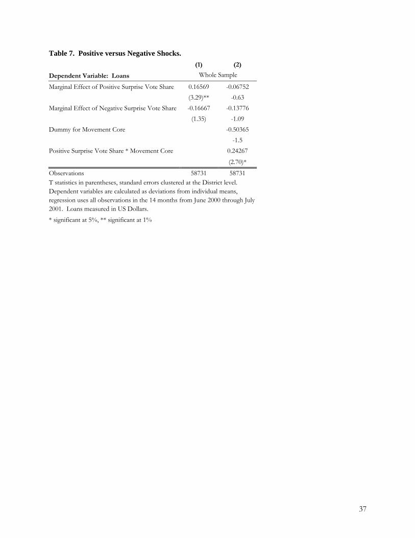
37

Table 7. Positive versus Negative Shocks.   (1) (2)

Dependent Variable: Loans Whole Sample

Marginal Effect of Positive Surprise Vote Share 0.16569 -0.06752 (3.29)** -0.63 Marginal Effect of Negative Surprise Vote Share -0.16667 -0.13776 (1.35) -1.09 Dummy for Movement Core -0.50365 -1.5 Positive Surprise Vote Share * Movement Core 0.24267

(2.70)*

Observations 58731 58731 T statistics in parentheses, standard errors clustered at the District level. Dependent variables are calculated as deviations from individual means, regression uses all observations in the 14 months from June 2000 through July 2001. Loans measured in US Dollars. * significant at 5%, ** significant at 1%  

38

Table 8. Robustness Check. Dependent Variable: Loans. (1) (2) (3)

Surprise Vote Share, 1 month prior to election 0.057 0.057 (1.27) (1.27) Surprise Vote Share, month of election 0.113 0.114 0.115 (2.12)* (2.21)* (2.20)* Surprise Vote Share, 1 month after election -0.034 -0.034

(0.24) (0.24)

Number of Observations: 58,731 58,731 58,731 T statistics in parentheses, standard errors clustered at the District level. Dependent variables are calculated as deviations from individual means, regression uses all observations in the 14 months from June 2000 through July 2001. Election was March 15 2001; month before election refers to loans made Feb15-Mar 14; month of election refers to Mar 15-Apr 15, month after election refers to Apr 15-May 15. Loans are in US Dollars. * significant at 5%, ** significant at 1%

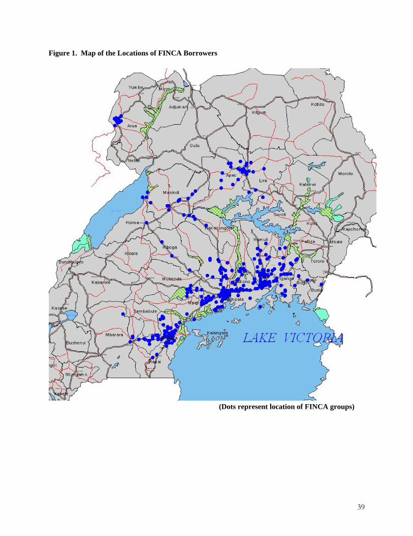
39

Figure 1. Map of the Locations of FINCA Borrowers

(Dots represent location of FINCA groups)

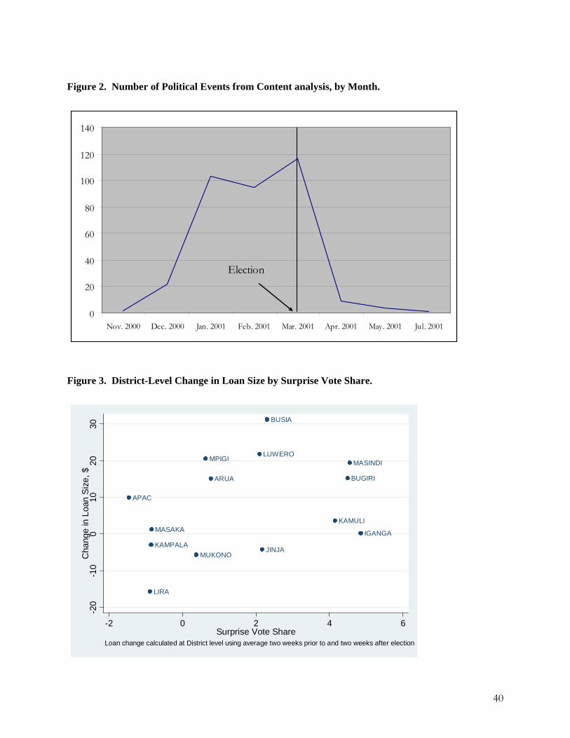
40

Figure 2. Number of Political Events from Content analysis, by Month.

0

20

40

60

80

100

120

140

Nov. 2000 Dec. 2000 Jan. 2001 Feb. 2001 Mar. 2001 Apr. 2001 May. 2001 Jul. 2001

Election

Figure 3. District-Level Change in Loan Size by Surprise Vote Share.

APAC

ARUA BUGIRI

BUSIA

IGANGA

JINJAKAMPALA

KAMULI

LIRA

LUWERO

MASAKA

MASINDIMPIGI

MUKONO

-20

-10

010

2030

Cha

nge

in L

oan

Siz

e, $

-2 0 2 4 6Surprise Vote Share

Loan change calculated at District level using average two weeks prior to and two weeks after election

41

Figure 4. Effects of the Surprise Vote Share as ‘Window’ Length is Increased:

42

Figure 5. Temporal Pattern of Loans around Election.

-30

-25

-20

-15

-10

-5

0

5

10

15

-6 -5 -4 -3 -2 -1 0 1 2 3 4 5 6

Weeks from Election

Dev

iati

ons

from

Ave

rage

LoansLower 95Upper 95

Figure 6. Temporal Pattern of Savings around Election.

-12

-10

-8

-6

-4

-2

0

2

4

6

-6 -5 -4 -3 -2 -1 0 1 2 3 4 5 6

Weeks from Election

Dev

iati

ons

from

Ave

rage

SavingsLower 95Upper 95