using exponential smoothing methods for modelling and ... · using exponential smoothing ......

Bachelor thesis

Using Exponential SmoothingMethods for Modelling and

Forecasting Short-Term ElectricityDemand

By

Michelle de Ruiter, 414429

Erasmus School of Economics

Bachelor Econometrics and Operations Research

Bachelor thesis [programme: Business Analytics and Quantitative Marketing]

Project supervisor: Dr. M. Zhelonkin

Second assessor: Dr. M. van de Velden

Rotterdam, 2 July 2017

i

Abstract

In this paper different exponential smoothing methods are considered for modelling and forecastingshort-term electricity demand in England and Wales. The time series contains half-hourly time periodsand two seasonalities can be observed – one within each day and one within each week. Both sea-sonalities are modelled separately with the Holt-Winters methods. The double seasonal Holt-Wintersmethod introduced by Taylor (2003) accommodates both seasonal patterns. An autoregressive modelis fitted to the residuals in order to deal with first-order autocorrelation. In addition, a model for mul-tiple seasonal (MS) processes introduced by Hyndman et al. (2008) is used, which divides the seasonalcomponent into several sub-cycles and allows for the seasonal sub-cycles to be combined. This reducesthe amount of seed values to be estimated. Moreover, the MS process allows for the seasonal terms tobe updated more than once during a seasonal cycle. Although the MS process with three combinedsub-cycles reduces the amount of seed values to be estimated and gives accurate forecasts, the doubleseasonal Holt-Winters method outperforms the other methods in forecasting the short-term electricitydemand.

ii

Contents

1 Introduction 1

2 Literature review 3

3 Data 4

4 Methodology 64.1 Exponential smoothing . . . . . . . . . . . . . . . . . . . . . . . . . . . . . . . . . . . . . 64.2 Holt-Winters method . . . . . . . . . . . . . . . . . . . . . . . . . . . . . . . . . . . . . . 6

4.2.1 Standard Holt-Winters method . . . . . . . . . . . . . . . . . . . . . . . . . . . . 64.2.2 Double seasonal Holt-Winters method . . . . . . . . . . . . . . . . . . . . . . . . 74.2.3 The additive formulation . . . . . . . . . . . . . . . . . . . . . . . . . . . . . . . 8

4.3 Multiple seasonal (MS) processes . . . . . . . . . . . . . . . . . . . . . . . . . . . . . . . 94.3.1 The seasonal components of the Holt-Winters methods . . . . . . . . . . . . . . . 94.3.2 The seasonal component of the MS process . . . . . . . . . . . . . . . . . . . . . 94.3.3 The model for the MS process . . . . . . . . . . . . . . . . . . . . . . . . . . . . 104.3.4 Model restrictions . . . . . . . . . . . . . . . . . . . . . . . . . . . . . . . . . . . 114.3.5 Model selection . . . . . . . . . . . . . . . . . . . . . . . . . . . . . . . . . . . . . 11

4.4 Estimation and prediction . . . . . . . . . . . . . . . . . . . . . . . . . . . . . . . . . . . 124.5 Residual autocorrelation . . . . . . . . . . . . . . . . . . . . . . . . . . . . . . . . . . . . 13

5 Results 145.1 Holt-Winters without AR(1) adjustment . . . . . . . . . . . . . . . . . . . . . . . . . . . 145.2 Holt-Winters with AR(1) adjustment . . . . . . . . . . . . . . . . . . . . . . . . . . . . . 155.3 The MS processes . . . . . . . . . . . . . . . . . . . . . . . . . . . . . . . . . . . . . . . . 17

5.3.1 Model selection . . . . . . . . . . . . . . . . . . . . . . . . . . . . . . . . . . . . . 175.3.2 Forecasting and comparison . . . . . . . . . . . . . . . . . . . . . . . . . . . . . . 21

6 Discussion and Conclusion 23

Appendices 24A From error correction form to component form . . . . . . . . . . . . . . . . . . . . . . . 24B Formulas for h-step ahead forecasts for models that include AR(1) term . . . . . . . . . 25C Sample autocorrelation plots of the Holt-Winters methods . . . . . . . . . . . . . . . . . 26D Parameter estimates of model selection procedures . . . . . . . . . . . . . . . . . . . . . 27

D.1 The MS process with multiplicative seasonality and no adjustment for autocor-relation. . . . . . . . . . . . . . . . . . . . . . . . . . . . . . . . . . . . . . . . . . 27

D.2 The MS process with multiplicative seasonality and adjustment for autocorrelation. 27D.3 The MS process with additive seasonality and adjustment for autocorrelation. . . 28

References 29

1

1 Introduction

Short-term electricity demand forecasting has become increasingly popular over the last decades. Ac-curate forecasts are very important for energy suppliers in order to operate and schedule such that thecosts are minimized.

A data set provided by the National Grid is used that contains twelve weeks of half-hourly de-mand for electricity in England and Wales. The first eight weeks will be used to estimate the modelparameters and the last four weeks are used for the evaluation of the forecasts. The series containstwo seasonalities, one within each week and one within each day. These seasonal cycles have to becaptured using accurate forecasting methods. The multiplicative seasonal ARIMA model is a widelyused benchmark approach for this purpose. Taylor (2003) introduced the double seasonal ARIMAmodel which is able to capture both seasonalities in the short-term electricity demand data. An al-ternative and very competitive method for modelling short-term electricity demand are exponentialsmoothing methods, which have become increasingly popular because of their accuracy. Exponentialsmoothing methods assign exponentially decreasing weights to the observations, which means thatolder observations are given relatively less weight than more recent observations. Holt-Winters is awidely used exponential smoothing method for forecasting short-term electricity demand. However,the standard Holt-Winters method can only accommodate one seasonal pattern. In this paper, thedouble seasonal Holt-Winters method introduced by Taylor (2003) will be used to forecast the timeseries. Three approaches are given; the standard Holt-Winters for within-day seasonality, the standardHolt-Winters for within-week seasonality, and the double seasonal Holt-Winters method that capturesboth seasonalities. In addition, these models will be estimated using a simple autoregressive (AR)model that is fitted to the one-step ahead forecast errors. This is suggested by Chatfield (1987) inorder to deal with first-order autocorrelated errors.

There are two variations of the Holt-Winters method, the multiplicative and the additive formula-tion. Taylor (2003) only models the electricity demand with the multiplicative formulation, which isused when the seasonal variation depends on the mean level of the time series. The second formulationis the additive formulation, where the seasonal variation is independent of the current mean level. Be-cause the seasonal variations are roughly constant through the series, the additive formulation of thedouble seasonal Holt-Winters method will also be used to model and forecast the electricity demand.

The electricity demand data in England and Wales show clearly different patterns for the weekdaysand the weekends. When modelling the electricity demand, Taylor (2003) assumes the same intra-day cycle for all days of the week. However, the demand for electricity at, for example, Mondaythrough Friday shows clearly different patterns than at Saturday and Sunday. Therefore, the modelfor multiple seasonal (MS) processes introduced by Hyndman et al. (2008) will be incorporated tomodel and forecasts the short-term electricity demand. This model can pick up the similarities fortime periods between different days, it reduces the number of parameters to be estimated and it allowsfor more flexibility in updating the seasonal components. Moreover, Hyndman et al. (2008) found thathis MS model produced more accurate forecasts than the double seasonal Holt-Winters model whenforecasting hourly utility demand.

The main aim of this paper is to use exponential smoothing methods to model the short-termelectricity demand in England and Wales and provide forecasts as accurate as possible. Taylor (2003)showed that his double seasonal Holt-Winters method is a very good candidate for forecasting this timeseries. However, Taylor (2003) uses the same intra-day cycle for all days of the week and therefore,a more efficient approach would be the multiple seasonal processes introduced by Hyndman et al.(2008), which relaxes some of the assumptions of the Holt-Winters methods. Moreover, Hyndman etal. (2008) found that his multiple seasonal process produced more accurate forecasts for his utility loadand traffic flows data than the double seasonal Holt-Winters model.

The paper is structured as follows. Section 2 describes the main results of the researches of Taylor(2003) and Hyndman et al. (2008) and some examples of which methods other researches have beenused to model complex seasonal patterns. In Section 3 the data of short-term electricity demand isdescribed. The time series is decomposed into the seasonal, trend and remainder component in order

2

to explain the most important features of the data. In Section 4 the different models and techniquesare described starting with a basic explanation of exponential smoothing in Section 4.1. In Section4.2 the Holt-Winters for within-day and within-week seasonality and the double seasonal Holt-Wintersmethod are explained. The additive formulation is also addressed. Section 4.3 explains the multipleseasonal process introduced by Hyndman et al. (2008). The estimation and forecasting procedure ofall methods is explained in Section 4.4 and Section 4.5 describes how an AR(1) model is fitted tothe residuals. Empirical analysis is done in Section 5, where the models described in Section 4 areincorporated and used to model and forecast the short-term electricity demand. A discussion andconclusion of the research is given in Section 6.

3

2 Literature review

A lot of research about time series with multiple seasonal patterns has already been done in manypublished papers, such as Taylor (2003), Hyndman et al. (2008) and Taylor (2010). A widely usedbenchmark approach for modelling seasonal time series is the ARIMA model of Box, Jenkins, andReinsel (1993). Taylor (2003) introduced the double seasonal ARIMA model which is able to capturetwo seasonalities. Furthermore, exponential smoothing methods, which are the central modellingtechniques used in this paper, are very popular in order to model time series with multiple seasonalities.

Taylor (2003) modelled the half-hourly electricity demand in England and Wales using four meth-ods, Holt-Winters for within-day seasonality, Holt-Winters for within-week seasonality, double seasonalHolt-Winters and the double seasonal ARIMA model. These first three methods will be explained andincorporated in this paper. Taylor (2003) fitted an autoregressive model to the residuals in order todeal with autocorrelated errors. He concludes that the double seasonal Holt-Winters methods withAR(1) adjustments outperforms the double seasonal ARIMA model and therefore, the double seasonalARIMA model will not be considered in this paper as exactly the same data is used.

Taylor (2003) uses the multiplicative version of the double seasonal Holt-Winters method, wherethe seasonality is estimated by smoothing the ratio of the observed value to the product of the locallevel and the local seasonal index. Also, the level equation makes sure that the series is seasonallyadjusted. This multiplicative method is much more common, and is used when the seasonal variationsincrease with the mean level of the series. However, another formulation involves additive seasonalityas explained in Hyndman and Athanasopoulos (2012). In this method, the series is seasonally adjustedby subtracting the seasonality in the level equation and the seasonality is estimated by smoothing thedifference of the observed value, the local level and the trend. The additive version is used whenthe seasonal variations are roughly constant through the series. Because this seems the case forthe electricity demand, also the additive version of the double seasonal Holt-Winters method will beinvestigated in this paper.

Multivariate modelling could be considered as in Taylor and Buizza (2003) which investigate the useof weather ensemble predictions in electricity demand forecasting. However, this paper will only con-sider univariate modelling approaches. Although weather variables such as temperature, the amountof rainfall and wind speed play a very important role in the demand for electricity according to Taylorand Buizza (2003), Taylor (2003) states that univariate methods seem to be sufficient for modellingsuch short lead times. This is due to the fact that most of the time weather variables change smoothlyover time rather than abrupt.

Other researchers that used exponential smoothing methods to model complex seasonalities arefor example De Livera, Hyndman, and Snyder (2010), who introduced a model that is able to handlenon-integer periods, high frequency multiple seasonal patterns and dual calender affects. Also Souza,Barros, and de Miranda (2007) use double seasonal exponential smoothing methods that account forholidays and temperature effects. However, for simplicity the data used in this paper contains noirregular days such as holidays.

Also Hyndman et al. (2008) make use of the Holt-Winters and the double seasonal Holt-Wintersmethods for modelling hourly data for both utility loads and traffic flows. They introduce a newmultiple seasonal (MS) process, which allows for each day to have its own hourly pattern by makinguse of different sub-cycles. An example for the utility loads is that they can generate one commonsub-cycle for Monday till Thursday and one common sub-cycle for Friday till Sunday. This will reducethe number of initial values and parameters to be estimated. In contrast to the double seasonalHolt-Winters method introduced by Taylor (2003), this methods allows for the seasonal terms tobe updated more than once during a seasonal cycle. Also, there is more flexibility in updating theseasonal components because the model allows for different smoothing parameters for different sub-cycles. Hyndman et al. (2008) concludes that the forecasts with this MS process are more accuratethan the double seasonal Holt-Winters method, when applied to the utility load and traffic flowsdata. Therefore, this paper will also incorporate this MS process to model and forecast the short-termelectricity demand.

4

3 Data

A time series provided by the National Grid is used which contains the demand of short-term electricityin England and Wales from Monday 5 June 2000 to Sunday 27 August 2000, which are exactly 12weeks. The data set is short-term in the sense that it contains 4032 observations, which means thatthere are 12 weeks of half-hourly demand for electricity. For simplification, this period is chosen as itcontains no special days, such as holidays. The univariate methods discussed in this paper will not beable to give reasonable forecasts for such data, as demand at these special days are very different from”regular” days. The time series is plotted in the top panel of Figure 3.1.

Figure 3.1: STL-decomposition of the time series of short-term electricity demand.

Figure 3.2: Two weeks of half-hourly electricity demand in England and Wales from Monday 5 June 2000 to Sunday18 June 2000.

5

Figure 3.2 shows the short-term electricity demand for only a fortnight in June 2000. This figuresshows clearly two seasonalities, a within-day seasonality and a within-week seasonality. The within-day seasonal cycle, which has a duration of 48 half-hour periods, can be observed because the demandat a particular time period in one day is similar to the demand at the same time period on anotherday. Particularly the weekdays show similar daily seasonal patterns. The weekends however show adifferent pattern than the weekdays. Moreover, every week the same seasonal pattern occurs. Thislonger weekly seasonal cycle has a duration of 336 half-hour periods and seems to dominate the seasonalvariation in the data.

To further explore the time series, a STL-decomposition is performed, which is a method to decom-pose a time series. The abbreviation STL means ”Seasonal and Trend decomposition using Loess” andis developed by Cleveland, Cleveland, McRae, and Terpenning (1990). The decomposition is shownin the last three panels of Figure 3.1. The bars at the right hand side of each graph allow to comparethe magnitudes of each component. The bar on the seasonal panel is almost as large as the bar onthe data panel, which indicates that the seasonal component dominates the variation in the data. Thebar on the trend panel shows that the trend has not much influence on the variation in the data. Thetrend panel shows a clear downward pattern around weeks eight to ten, which is slightly noticeable inthe data panel.

The first eight weeks of the time series will be used for estimation of the model parameters. Thisamounts to the first 2688 half-hourly time periods as estimation sample. The remaining four weekswill be used for estimation, which amounts to the last 1344 observations of the data set.

6

4 Methodology

4.1 Exponential smoothing

One can use simple methods to generate forecasts for time series, such as the naıve method, whichjust takes the last observation of the series as the forecasts, or the average method, which uses theaverage of all observations as the forecasts. These simple methods thus give equal weights to all of theforecasts. Most of the time, this does not give very reliable predictions. A better approach is usuallyto assign more weight to more recent observations and less weight to observations further in the past.An example of this kind of forecast is

XT+1|T = αXT + α(1− α)XT−1 + α(1− α)2XT−2 + ..., (1)

where 0 ≤ α ≤ 1 is the smoothing parameter. As can be seen from Equation 1 the weights decreaseexponentially and α determines at which rate they decrease. When α is close to 1, relatively moreweight is assigned to more recent observations and when α is close to 0, relatively more weight is givento observations further in the past. This is the general idea behind exponential smoothing.

Simple exponential smoothing (SES) can be used for time series that contain no trend nor season-ality. In this paper, the exponential smoothing methods will be formulated in the so-called componentform. The component form for SES is

Forecast equation: Xt+1|t = St,

Level equation: St = αXt + (1− α)St−1.

This form contains only one component, which is the smoothing equation for the level St. Thisequation can be rewritten in the error correction form, which will make clear what the role of α is. Wecan rewrite St as

St = αXt + (1− α)St−1

= αXt + St−1 − αSt−1= St−1 + α(Xt − St−1)

= St−1 + αet,

where et = Xt − St−1 is the one-step within-sample forecast error at time t, t = 1, ..., T . Now wecan see that the level is ”smoother” when α comes close to zero, because small weight is given to theerror et.

This was a short explanation of how the simplest form of exponential smoothing methods works.However, the short-term electricity demand data does contain a trend and seasonality. Holt (1957)and Winters (1960) introduced an exponential smoothing method that accounts for both trend andseasonality, which will be referred to as the standard Holt-Winters method. Taylor (2003) extendedthis method to the double seasonal Holt-Winters method, which is able to capture both seasonalities.These methods will be explained in Section 4.2.

4.2 Holt-Winters method

4.2.1 Standard Holt-Winters method

In order to deal with the trend and the seasonal components in the time series of short-term electricitydemand, the standard Holt-Winters method will be implemented. This method can only accommodateone seasonality. Therefore, the within-day (s=48) and the within-week (s=336) seasonalities will bemodelled separately.

7

The standard Holt-Winters method contains three components, one smoothing equation for thelevel, one for the trend and one for the seasonality. The component formulation of the multiplicativeHolt-Winters method is represented below. The same formulation as in Taylor (2003) is used.

Xt(h) = (St + hTt)It−s+h, (2a)

Level: St = α

(Xt

It−s

)+ (1− α)(St−1 + Tt−1), (2b)

Trend: Tt = β(St − St−1) + (1− β)Tt−1, (2c)

Seasonality: It = δ

(Xt

St

)+ (1− δ)It−s. (2d)

The h-step ahead forecasts Xt(h) are calculated using the smoothing equations for the level, thetrend and the seasonality. The level in Equation 2b is estimated by smoothing (1) the ratio of theobserved value and the seasonal index at exactly one seasonal cycle ago and (2) the sum of the previouslevel and the previous trend St−1 + Tt−1, where 0 ≤ α ≤ 1 is the smoothing parameter. The trendcomponent in Equation 2c is additive and is estimated by the weighted average of the first differencesof the level St−St−1 and the previous trend Tt−1. The smoothing parameter for the trend is 0 ≤ β ≤ 1.The seasonal index at time t in Equation 2d is estimated by the weighted average of (1) the ratio of theobserved value at time t and the level at time t and (2) the seasonal index exactly one seasonal cycleago. For example, when the within-day seasonality (s=48) for the electricity demand is modelled, theseasonal index at time t=50 will be estimated using the seasonal index exactly one day ago, at t=2.The smoothing parameter for the seasonality is 0 ≤ δ ≤ 1. The initial values for the level S0, the trend

T0 and the seasonal index I0 =[I−s, I−s+1, . . . , I0

]>are chosen the same as in the standard

implemented R function HoltWinters.R.

4.2.2 Double seasonal Holt-Winters method

Taylor (2003) proposed an extension of the standard Holt-Winters method in order to deal withtwo seasonalities. The double seasonal Holt-Winters method contains four components – one for thelevel, one for the trend and one for each seasonality. The method can be extended to three or moreseasonalities. The formulation of the multiplicative model in this paper is same as used by Taylor(2003) and is represented in the following equations:

Xt(h) = (St + hTt)Dt−s1+hWt−s2+h, (3a)

Level: St = α

(Xt

Dt−s1Wt−s2

)+ (1− α)(St−1 + Tt−1), (3b)


Seasonality 1: Dt = δ

(Xt

StWt−s2

)+ (1− δ)Dt−s1 , (3d)

Seasonality 2: Wt = ω

(Xt

StDt−s1

)+ (1− ω)Wt−s2 . (3e)

The h-step-ahead forecasts Xt(h) are now calculated using the level component, the trend compo-nent and the two seasonal indexes Dt and Wt, where Dt is the smoothing equation for the s1-periodseasonal cycle and Wt is the smoothing equation for the s2-period seasonal cycle. In this paper, s1 = 48for the within-day seasonality and s2 = 336 for the within-week seasonality. The level in Equation

8

3b is estimated using the weighted average of (1) the ratio of the observed value at time t and themultiplication of the two seasonal indices one seasonal cycle ago and (2) the sum of the previous leveland the previous trend. The trend component in Equation 3c is estimated in the same way as in thestandard Holt-Winters method. The smoothing parameters for the level and the trend are 0 ≤ α, β ≤ 1respectively. The within-day seasonal component Dt is estimated using the weighted average of (1)the ratio of the observed value at time t and the level at time t multiplied by the within-week seasonalindex exactly one week ago and (2) the within-day seasonal index exactly one day ago. The within-week seasonal component Wt is estimated using the weighted average of (1) the ratio of the observedvalue at time t and the level at time t multiplied by the within-day seasonal index exactly one dayago and (2) the within-week seasonal index exactly one week ago. The smoothing parameters for thewithin-day and within-week seasonal components are 0 ≤ δ, ω ≤ 1 respectively.

The initial values for the trend T0, the level S0, the within-day seasonal index

D0 =[D−s1 , D−s1+1, . . . , D0

]>and the within-week seasonal index

W0 =[W−s2 , W−s2+1, . . . , W0

]>are chosen the same as in Taylor (2003).

4.2.3 The additive formulation

Two variations of this method exist, the additive method and the multiplicative method.The Holt-Winters methods described above all involved multiplicative seasonality. However, an-

other formulation involves additive seasonal patterns. According to Hyndman and Athanasopoulos(2012) the choice of which method to use depends mostly on the seasonal variations. When theseare constant through the series, the additive method should be the best choice. When the seasonalvariations change proportional to the level of the time series, the multiplicative method is preferred.The latter is much more used for forecasting seasonal time series, but the series of electricity demandshows roughly constant seasonal variations, also the additive formulation will be investigated for thedouble seasonal Holt-Winters method. This formulation is represented below.

Xt(h) = St + hTt +Dt−s1+h +Wt−s2+h, (4a)

Level: St = α(Xt −Dt−s1 −Wt−s2) + (1− α)(St−1 + Tt−1), (4b)


Seasonality 1: Dt = δ(Xt − St −Wt−s2) + (1− δ)Dt−s1 , (4d)

Seasonality 2: Wt = ω(Xt − St −Dt−s1) + (1− ω)Wt−s2 . (4e)

The level component in Equation 4b is estimated by smoothing the difference of the observedvalue and the within-day and within-week seasonality one seasonal cycle ago instead of smoothing theratio of these components. The trend component in Equation 4c is the same as in Equation 3c forthe multiplicative formulation. The seasonal indices undergo the same change - instead of the ratio,the difference of the observed value, the level and the other seasonal index is used to estimate thecomponent. Also, the h-step ahead forecasts are calculated using addition instead of multiplication.Again, α, β, δ and ω are the smoothing parameters to be estimated.

9

4.3 Multiple seasonal (MS) processes

4.3.1 The seasonal components of the Holt-Winters methods

The Holt-Winters methods explained in Section 4.2 assume the same seasonal intra-day cycle for alldays of the week. The standard Holt-Winters method uses the seasonal cycle

It =[It, It−1, . . . , It−s+1

]>,

where s=48 (i.e. within-day seasonality) or s=336 (i.e. within-week seasonality). This model thusneeds to estimate s+2 different seed values – one for the level, one for the trend and s for the seasonalcomponent. Every seasonal term is updated once during the seasonal cycle of s time periods. Thismeans that for a daily cycle of length s=48 the seasonal terms are updated once every day and thatfor a weekly cycle of length s=336 the seasonal terms are updated once every week. Also, the modeluses the same smoothing parameter δ for each of the s seasonal terms during a particular cycle.

The double seasonal Holt-Winters method uses two seasonal cycles denoted by

Dt =[Dt, Dt−1, . . . , Dt−s1+1

]>for the within-day seasonality and

Wt =[Wt, Wt−1, . . . , Wt−s2+1

]>for the within-week seasonality. This model thus requires s1 +s2 +2 different seed values, where s1=48and s2=336. This means that 336 seasonal terms are updated once every week and an additional48 seasonal terms are updated once every day. Also in this model, the same smoothing parameter δfor the within-day seasonal terms and the same smoothing parameter ω for the within-week seasonalterms are used.

4.3.2 The seasonal component of the MS process

Hyndman et al. (2008) developed a model for a multiple seasonal process with the aim of updatingthe seasonal terms more than once during a seasonal cycle. This is done by relaxing some of theassumptions for the seasonal components of the standard and double seasonal Holt-Winters methodsdescribed above. The model allows to combine certain daily sub-cycles into one sub-cycle. For example,when we look at the data in the top panel of Figure 3.1, we can distinguish 7 different daily sub-cycles.However, the cycles of the weekdays seem very similar and we could combine these cycles into onesub-cycle. If the two sub-cycles of Saturday and Sunday are also combined, we end up with a seasonalcomponent that is divided into r = 2 sub-cycles. This is a large reduction in the amount of seasonalterms to be estimated. How this process exactly works is explained below.

First, the seasonal component with the initial seasonal terms is divided into r sub-cycles as follows

ci,0 = (Ii,−s1+1, Ii,−s1+2, . . . , Ii,−1, Ii,0)>

= (I−s1(r−i)−s1+1, I−s1(r−i)−s1+2, . . . , I−s1(r−i)−1, I−s1(r−i))>, (5)

where i = 1, . . . , r and r ≤ k = s2s1

. If we would choose r equal to k, the seasonal component would

be divided into k = s2s1

= 33647 = 7 daily sub-cycles. As we will see later in this paper, under certain

restrictions this amounts to the standard Holt-Winters method for within-week seasonality.The division of the initial seasonal component in Equation 5 can be extended for each time period

t as follows:

cit = (Ii,t, Ii,t−1, . . . , Ii,t−s1+1)>, (6)

where i = 1, . . . , r. Now, cit in Equation 6 contains at each time period t the current s1 seasonalterms for cycle i.

10

4.3.3 The model for the MS process

The model for multiplicative seasonality

Hyndman et al. (2008) uses the error correction form to represent the model for the multiple seasonalprocess. This form is explained in Section 4.1. In this paper, all models are represented in thecomponent form. A very similar model with additive trend and multiplicative seasonality that isrepresented in the component and the error correction form is stated in Hyndman andAthanasopoulos (2012), who provide various tables containing both formulations of various differentmodels. These tables are used to write the error correction formulation of the model of Hyndman etal. (2008) into the component form. The component formulation of the model for the multipleseasonal process with multiplicative seasonality is

Xt(h) = (St−1 + hTt−1)d>t It−s1+h, (7a)

Level: St = α

(Xt

d>t It−s1

)+ (1− α)(St−1 − Tt−1), (7b)

Trend: Tt = β∗(St − St−1) + (1− β∗)Tt−1, (7c)

Seasonality: It = Γdt

(Xt

St−1 + Tt−1

)+ It−s1 − Γdtd

>t It−s1 , (7d)

where It =[I1,t, I2,t, . . . , Ir,t

]>and dt =

[d1,t, d2,t, . . . , dr,t

]>, where

di,t =

{1 if time period t occurs within sub-cycle i;

0 otherwise.(8)

Γ is a matrix that contains for each sub-cycle the smoothing parameters γij , where i, j = 1, . . . , r. Inthis way, the model allows for different smoothing parameters for different sub-cycles. The diagonalelements γii are used to update seasonal terms during time periods of the same sub-cycle, whereasthe off-diagonal elements γij are used to update seasonal terms during time periods in another

sub-cycle. We will denote this model by MS(r; s1, s2). The h-step ahead forecasts Xt(h) arecalculated similarly as in Taylor (2003), because this allows for easy comparison of the Holt-Wintersmethods from Section 4.2 and the MS processes.

The model for additive seasonality

Besides the MS process for multiplicative seasonality, Hyndman et al. (2008) introduced the MSprocess for additive seasonality. The Holt-Winters methods described above are implemented forboth the multiplicative and the additive seasonality, so the MS process will also be adapted foradditive seasonal patterns. Instead of the error correction formulation according to Hyndman et al.(2008), the component formulation will be used to represent the model. The derivation from theerror correction form used by Hyndman et al. (2008) to the component form can be found inAppendix A. The MS process for additive seasonality is very similar as the model in Equations 7 andcan be represented as follows:

Xt(h) = St−1 + hTt−1 + d>t It−s1+h, (9a)

Level: St = α(Xt − d>t It−s1) + (1− α)(St−1 − Tt−1), (9b)

Trend: Tt = β∗(St − St−1) + (1− β∗)Tt−1, (9c)

Seasonality: It = Γdt(Xt − St−1 − Tt−1) + It−s1 − Γdtd>t It−s1 . (9d)

11

4.3.4 Model restrictions

The matrix of smoothing parameters for the different sub-cycles can become quite large when theamount of different sub-cycles r increases, because Γ is an r× r matrix and thus contains r2 elements.Hyndman et al. (2008) imposes three restrictions on Γ to reduce the number of parameters. Someof these restrictions will lead to the standard or double seasonal Holt-Winters method described inSection 4.2.

First of all, Hyndman et al. (2008) divide the smoothing parameters in Γ into diagonal elementsand off-diagonal elements as follows:

γi,j =

{γ∗1 if i = j;

γ∗2 if i 6= j.(10)

The three restrictions of interest according to Hyndman et al. (2008) are

• Restriction 1: γ∗1 6= 0 and γ∗2 = 0

• Restriction 2: γ∗1 = γ∗2

• Restriction 3: Equivalent to Equation 10

Restriction 1 does not allow the seasonal terms in a particular sub-cycle to be updated duringanother sub-cycle. Moreover, when r = k this restricted model is the same as the standard Holt-Winters model for within-week seasonality, where γ∗1 = δ in Equation 2d. If the seed values for thedifferent sub-cycles would be equal to each other, the model with restriction 2 would be identical to thestandard Holt-Winters for within-day seasonality. However, the seed values of the sub-cycles are rarelyidentical in modelling this multiple seasonal process. This restricted model will allow the seasonal termsin a sub-cycle to be updated during another sub-cycle, although using the same smoothing parameter.Restriction 3 allows for different smoothing parameters when updating seasonal sub-cycles during thesame sub-cycle and other sub-cycles. Moreover, when r = k this restricted model is equivalent to thedouble seasonal Holt-Winters method, where γ∗1 = δ + ω and γ∗2 = δ in Equations 3d and 3e. A briefoverview of the amount of smoothing parameters and seed values to be estimated for all the models isgiven in Table 1.

Table 1: Smoothing parameters and seed values required for each model

Model Smoothingparameters

Seed values

Holt-Winters for within-day seasonality 3 s1 + 2Holt-Winters for within-week seasonality 3 s2 + 2Double seasonal Holt-Winters 4 s1 + s2 + 2MS(r; s1, s2) r2 + 2 rs1 + 2MS(r; s1, s2) with Restriction 1 3 rs1 + 2MS(r; s1, s2) with Restriction 2 3 rs1 + 2MS(r; s1, s2) with Restriction 3 4 rs1 + 2

4.3.5 Model selection

In order to select the most appropriate model we have to choose the number of different sub-cyclesr and the restriction for the smoothing parameters belonging to the seasonal component. The modelselection is performed based on the two step selection procedure by Hyndman et al. (2008).

12

The first step involves the decision of which value of r to use. To select possible values of r, theseasonal terms of the last week of the estimation sample, estimated with the double seasonal Holt-Winters model, are plotted. From this plot it will be clear which possible daily seasonal cycles can becombined into one sub-cycle.

From the estimation sample consisting of n=2688 time-periods the last 20% of the time-periodsrounded to the nearest multiple of whole weeks are withheld. This amounts to q = 672 time-periods or2 weeks of data for the short-term electricity demand. Next, the parameters of the different MS(r; 48,336) will be estimated using observations 1 to n− q by minimizing the one-step ahead sum of squarederrors. For each model, the MAPE(1) for the one-step ahead forecasts for observations n− q + 1 to nis calculated as follows:

MAPE(1) =100

q

n∑t=n−q+1

∣∣∣Xt − Xt

Xt

∣∣∣. (11)

.The value of r is picked from the model with the lowest MAPE(1) value.The second step involves choosing the restrictions on Γ. The value of r from the first step is selected

and the one-step ahead forecasts for periods n − q + 1 till n are made for Restriction 1, 2, 3 and norestriction. The restriction that produces the lowest MAPE(1) is imposed in the MS process.

4.4 Estimation and prediction

The estimation and forecasting procedure is the same for all the methods discussed in Sections 4.2and 4.3. The first eight weeks of the data are used for the estimation of the model parameters. Forthe series of half-hourly demand this amounts to the first n = 2688 observations. The one-step aheadforecasts ˆXt+1 are calculated for the estimation sample. These forecasts are used to compute theone-step ahead forecast errors et+1 as follows:

et+1 = Xt+1 − ˆXt+1, (12)

where t=0,...,n − 1. The smoothing parameters are optimized by minimizing the sum of squarederrors (SSE), as in the following equation:

SSE =

n∑t=1

e2t . (13)

When the values for the smoothing parameters are optimized, these values can be used to forecastthe electricity demand for the remaining four weeks, which is also called the post-sample period. Thisperiod consists of observations at t = n + 1, ..., T , which makes a total of p=1344 observations. Theh-step ahead forecasts are calculated for h = 1, ..., s1, where s1=48 is the within-day seasonality. Theseforecasts Xt+h can be saved in a matrix, where the rows represent h=1,...,48 and the columns representt=2688,...,4031. This matrix looks as follows:

X2689 X2690 X2691 . . . X4031 X4032

X2690 X2691 X2692 . . . X4032 −...

......

. . ....

...

X2736 X2737 X2738 . . . − −

A widely used measure for comparing the post-sample forecast accuracy is the Mean Absolute

Percentage Error (MAPE). The matrix of h-step ahead forecasts allows us to calculate the MAPE(h)values for h = 1, . . . , s1 as follows:

MAPE(h) =100

p− (h− 1)

T−h∑t=n

∣∣∣Xt+h − Xt+h

Xt+h

∣∣∣. (14)

13

4.5 Residual autocorrelation

According to Gardner (1985) the forecasts from exponential smoothing methods can be improved byintroducing an AR(1) model to the one-step ahead forecast errors. Taylor (2003) uses this adjustmentin the Holt-Winters methods because he found sizeable first-order autocorrelated errors. The AR(1)model is as follows:

et = φet−1 + ζt, (15)

where φ is the model parameter to be estimated and ζt is white noise. The h-step-ahead forecastsare modified by adding the term φket, where φ is estimated with the estimation sample. This meansthat the formulas of the h-step-ahead forecasts for all models change. For example, the h-step aheadforecast for the standard Holt-Winters model in Equation 2a becomes

Xt(k) = (St + kTt)It−s+k + φket

= (St + kTt)It−s+k + φk{Xt − (St−1 + Tt−1)It−s}. (16)

The modified h-step ahead forecasts for the other models can be found in Appendix B.

14

5 Results

5.1 Holt-Winters without AR(1) adjustment

The optimal smoothing parameter values are calculated by minimizing the sum of squared one-stepahead forecast errors as explained in Section 4.4. The optimized values for the Holt-Winters methodwithout the AR(1) adjustment are shown in Table 2. The estimated parameter α takes values closeto 1, which means that all methods give relatively more weight to more recent observations. Asexplained in Section 3 the variability in the estimation sample is dominated by the seasonality, ratherthan the trend. This trend constantly takes small values when modelling Holt-Winters for within-weekseasonality and double seasonal Holt-Winters. This explains the zero values for β for these two methodsin Table 2. However, in the Holt-Winters for within-day seasonality the optimized parameter β forthe trend takes the larger value of 0.853, which is accompanied by the smoothed trend taking highlyvarying values. According to Taylor (2003), Holt-Winters for within-day seasonality incorporated thishighly varying trend because it is unable to model the within-week seasonality.

Table 2: Holt-Winters smoothing parameters optimized from estimation sample. There is no adjustment for autocor-relation in the residuals of the methods.

Level α Trend β Within-dayseasonality δ

Within-weekseasonality ω

Holt-Winters for within-day seasonality 0.986 0.853 1.000 -Holt-Winters for within-week seasonality 0.831 0.000 - 1.000Double seasonal Holt-Winters 0.881 0.000 0.831 1.000

For each of the three methods the MAPE values for 48 lead times are calculated as explained inSection 4.4. In Figure 5.1 the MAPE results for the different Holt-Winters methods are compared.The MAPE values for Holt-Winters for within-day seasonality increase at such a large rate that onlythe MAPE values until 2-step ahead forecasts are plotted. This large increase in MAPE values isdue to the fact that this method only accommodates the within-day seasonality, while the data in thetop panel of Figure 3.1 also shows a within-week seasonal pattern, which dominates the variation inthe data. Therefore, Holt-Winters for within-week seasonality shows much better results. The doubleseasonal Holt-Winters method shows better forecast accuracy for lead times up to 9 and beyond 39,which indicates that taking both seasonalities in account will probably improve the forecast accuracy.

Figure 5.1: Comparison of the out of sample MAPE(h) results for the Holt-Winters methods.

15

The forecasts can be improved by fitting an AR(1) model to the residuals, which is explained inSection 4.5. The one-step ahead forecast errors for all three Holt-Winters methods show significantautocorrelation, which means that the residuals contain some information that can be exploited toobtain more accurate forecasts. Figure 5.2 shows the sample autocorrelation function (ACF) for theone-step ahead forecast errors in the estimation sample for double seasonal Holt-Winters. Only thedouble seasonal Holt-Winters method will be considered here because this method is likely to producethe most accurate forecasts of the three Holt-Winters methods. The ACF plots of the Holt-Wintersfor within-day and within-week seasonality can be found in Appendix C. The ACF plot in Figure 5.2shows spikes at various lags, which means that the forecasts are not optimal and can be improved.

Figure 5.2: The sample autocorrelation plot of the one-step ahead forecast errors obtained from estimating theestimation sample with the double seasonal Holt-Winters method.

5.2 Holt-Winters with AR(1) adjustment

Because of the first-order autocorrelation of the one-step ahead forecast errors, an AR(1) model is fittedto these errors. The estimation of the parameters is done in a single stage, which is more efficientthan a two-stage estimation procedure according to Chatfield (1987). The parameters are optimizedby minimizing the sum of squared one-step ahead forecast errors from the estimation sample, wherean AR(1) model is fitted to the errors. The optimized parameters are shown in Table 3. The valuesof the estimated level parameter α are much smaller for Holt-Winters for within-week seasonality anddouble seasonal Holt-Winters than the value for α in the models without AR(1) adjustment. It seemsthat the smoothing equation for the level has almost been replaced by the fitted AR(1) model for the

residuals. The estimated trend parameter β now also takes the value zero for Holt-Winters for within-day seasonality. The parameters δ and ω have decreased substantially for all of the three multiplicativeseasonal Holt-Winters methods compared to those in Table 2.

In Figure 5.3 the MAPE results are shown for the three multiplicative Holt-Winters methods forlead times up to a day-ahead. Again, the MAPE results for the Holt-Winters for within-day seasonalityare very poor, which can be explained by the dominance of the within-week seasonality in the variationof the data. However, the results for Holt-Winters for within-week seasonality and the double seasonalHolt-Winters have improved compared to the models without the AR(1) adjustment for the forecasterrors. The double seasonal Holt-Winters method outperforms the Holt-Winters for within-day and

16

Table 3: Holt-Winters smoothing parameters optimized from estimation sample. The methods include an AR(1) modelfor the residuals.

Level α Trend β Within-dayseasonality δ

Within-weekseasonality ω

AR φ

Holt-Winters for within-day seasonality 0.803 0.000 0.689 - 0.736Holt-Winters for within-week seasonality 0.013 0.000 - 0.416 0.924Double seasonal Holt-Winters 0.012 0.004 0.179 0.325 0.935Additive double seasonal Holt-Winters 0.000 0.000 0.362 0.344 0.986

within-week seasonality for all h-step ahead forecast errors.The additive formulation of the double seasonal Holt-Winters model gives almost identical per-

formances compared to the multiplicative version of the model. The estimates for the smoothingparameters β and δ for the additive formulation can be found in Table 3 and are slightly larger thanthose of the multiplicative version. Also the estimated parameter φ of the AR(1) model is slightlylarger. Figure 5.4 shows the MAPE(h) values for both the additive and the multiplicative double sea-sonal Holt-Winters methods. Most of the time the additive formulation gives more accurate forecaststhan the multiplicative formulation, although the improvement is almost nil.

Figure 5.3: Comparison of the out of sample MAPE(h) results for the three Holt-Winters methods including AR(1)model for the residuals.

Figure 5.5 shows the ACF plot of residuals from the multiplicative double seasonal Holt-Wintersmethod with AR(1) adjustment. The plot shows much less spikes at different lags than the ACFplot in Figure 5.2, which indicates that the AR(1) model for the residuals reduced the remainingautocorrelation. However, there still is some autocorrelation in the one-step ahead errors. The ACFplots of the residuals from the Holt-Winters method for within-day and within-week seasonality withAR(1) adjustment can be found in Appendix C.

17

Figure 5.4: Comparison of the MAPE results for the additive and multiplicative double seasonal Holt-Wintersmethods including AR(1) model for the residuals.

Figure 5.5: The sample autocorrelation plot of the one-step ahead forecast errors obtained from estimating theestimation sample with the double seasonal Holt-Winters method including AR(1) adjustment.

5.3 The MS processes

5.3.1 Model selection

The first step of selecting an appropriate model is to choose the value of r. In order to choose thisvalue, it has to be investigated which seasonal sub-cycles can be combined. To see which seasonalcycles could be combined, the seasonal terms for each day of the last week of the estimation sampleare plotted in Figure 5.6. The seasonal terms belong to the double seasonal Holt-Winters method,which is equivalent to the MS(7; 48, 336) model as explained in Section 4.3.4.

From Figure 5.6 it can be seen that the weekdays and the weekends show clearly different seasonal

18

Figure 5.6: The estimated half-hourly seasonal sub-cycles for each day of the last week of the estimation sample. Theseasonal term on the y-axis represents the seasonal terms in Equation 6, where r = 7.

patterns. Therefore, one possibility for combining the seasonal cycles is one common sub-cycle forMonday through Friday and one common sub-cycle for Saturday and Sunday. However, Saturday andSunday also show dissimilarities in the patterns. Therefore, a second approach involves one sub-cyclefor Monday through Friday and separate sub-cycles for Saturday and Sunday. Another interestingpattern is that of Monday and Friday. When the weekend has ended and Monday starts at 12:00AM, the seasonal terms take the same values as the weekend until 6:00 AM. After that, the patternbecomes the same as that of the weekdays. Moreover, when the weekend begins at Friday, the seasonalpattern of Friday changes from the same pattern as the weekdays to the seasonal values of the weekend.However, most of the time the patterns for Monday and Friday display similar patterns as Tuesdaytill Thursday. Therefore, the following MS processes are investigated:

• MS(2; 48, 336): A common sub-cycle for Monday through Friday and a common sub-cycle forSaturday and Sunday.

• MS(3; 48,336): A common sub-cycle for Monday through Friday and two separate sub-cycles forSaturday and Sunday.

The selection procedure for the model with multiplicative seasonality

The smoothing parameters of the multiplicative MS(2; 48, 336) and MS(3; 48, 336) processes areestimated using the first n− q = 2016 time periods (i.e. the first 6 weeks). The estimated parametervalues can be found in Appendix D.1. The one-step ahead forecasts are produced for observationsn− q + 1 = 2017 till n = 2688. The MAPE(1) values resulting from the one-step ahead forecasterrors for both methods are shown in Table 4. The MS(2; 48, 336) process gives a lower MAPE(1)value than the MS(3; 48, 336) process. Moreover, the MS(2; 48, 336) process only needs to estimate6 parameter values and 98 seed values, whereas the MS(3; 48, 336) process needs 11 parametersestimates and 146 seed values. Therefore, we continue with imposing the restrictions on the MS(2;

19

48, 336) model. The MAPE(1) values resulting from the one-step ahead forecasts produced by theMS(2; 48, 336) with the various restrictions are shown in Table 4. Imposing any of the threerestrictions does not improve the accuracy of the one-step ahead forecasts, because all MAPE(1)values are larger than that of the MS(2; 48, 336) model without any restrictions.

Table 4: Withheld sample MAPE(1) in MS model selection.

Model Restriction MAPE(1) Parameters Seed valuesStep 1 MS(2; 48, 336) none 1.757 6 98

MS(3; 48, 336) none 2.308 11 146Step 2 MS(2; 48, 336) 1 1.937 3 98

MS(2; 48, 336) 2 2.077 3 98MS(2; 48, 336) 3 1.981 4 98

Estimation of the MS(2; 48, 336) process using the estimation sample of the first n = 2688 (i.e.the first 8 weeks) gives the following parameter estimates:

α = 1.000, β∗ = 0.000 and Γ =

[0.497 0.0000.167 0.221

].

The estimated parameter for the level takes the maximum value of 1.000 which means that relativelymore weight is given to more recent observations. The estimated parameter β∗ for the trend takesthe value zero, which can be explained by the seasonality that dominates the variability in the data.The estimated smoothing parameters in Γ show that the seasonal sub-cycles are updated during timeperiods of the same sub-cycle, but also during time periods of the other sub-cycle. This can beexplained by writing the multiplicative MS(2; 48, 336) process as follows:

[I1,tI2,t

]=

[γ11 γ12γ21 γ22

] [d1,td2,t

](Xt

St−1 + Tt−1

)+

[I1,t−s1I2,t−s1

]−[γ11 γ12γ21 γ22

] [d1,td2,t

] [d1,t d2,t

] [I1,t−s1I2,t−s1

].

From this formulation it is easier to see that at a time period t the first sub-cycle for the weekdaysI1,t can be updated using the sub-cycle for the weekdays I1,t−s1 , but also using the sub-cycle forthe weekend I2,t−s1 . Moreover, the second sub-cycle for the weekend I2,t can be updated using thesub-cycle for the weekend I2,t−s1 , but also using the sub-cycle for the weekdays I1,t−s1 .

However, the sample autocorrelation function of the residuals from the in-sample one-step aheadforecasts show significant spikes at different lags. The ACF plot is shown in Figure 5.7. This indicatesthat there is remaining autocorrelation in the one-step ahead forecast errors. Therefore, an AR(1)model is fitted to the one-step ahead errors for the same reasons as with the Holt-Winters modelsdescribed in Sections 4.5 and 5.1. Again, the model selection procedure as described in Section 5.3.1is performed for the MS(2; 48, 336) and the MS(3; 48, 336) processes with the implementation of thedifferent restrictions. The results of the model selection procedure for the models with adjustment forautocorrelation are shown in Table 5. The estimated parameter values for each model can be foundin Appendix D.2. The MAPE(1) values have reduced substantially for all the considered models fromthose in Table 4. This means that the forecast accuracy for the withheld sample has improved byadjusting for the autocorrelation in the residuals. The model selection procedure in Table 5 showsthat the MS(2; 48, 336) without restrictions produces the lowest MAPE(1) value of 0.528.

Estimation of the MS(2; 48, 336) process without any restrictions and with adjustment for auto-correlated errors is done using the estimation sample of the first n = 2688 (i.e. the first 8 weeks) andgives the following parameter estimates:

α = 0.000, β∗ = 0.000, Γ =

[1.000 0.4080.917 0.505

]and φ = 0.925.

20

The estimated parameter values are similar to those of the Holt-Winters methods in Table 3.The smoothing equation for the level seems to be replaced by the AR(1) model, because α takes the

minimum value and φ almost reaches its maximum with a value of 0.925. The estimated parameter forthe trend is zero and the seasonal sub-cycles are updated during time periods of the same sub-cyclesand during time periods of the other sub-cycle.

The ACF plot of the one-step ahead forecasts errors from the estimation sample is shown in Figure5.8. The amount of spikes has reduced substantially, which means that the AR(1) model for theresiduals reduced the remaining autocorrelation. However, the ACF plot in Figure 5.8 still showssome spikes, especially around lag 14. This indicates that there is still some autocorrelation left in theresiduals.

Figure 5.7: The ACF plot of the residuals from theMS(2; 48, 336) process without AR(1) term.

Figure 5.8: The ACF plot of the residuals from theMS(2; 48, 336) process with AR(1) term.

Table 5: Withheld sample MAPE(1) in MS model selection with AR adjustment.


MS(3; 48, 336) none 0.614 12 146Step 2 MS(2; 48, 336) 1 0.551 4 98

MS(2; 48, 336) 2 0.690 4 98MS(2; 48, 336) 3 0.553 5 98

The selection procedure for the model with additive seasonality

So far, only the MS processes that involve multiplicative seasonality have been considered. However,the results in Section 5.2 have shown slight improvements when modelling the electricity demandwith the additive formulation of the double seasonal Holt-Winters method rather than themultiplicative version. Therefore, the model selection procedure for the MS process with additiveseasonality will also be considered. The models include adjustment for autocorrelated errors byadding an AR(1) term. The additive MS processes without adjustment for autocorrelation are alsoconsidered, but they did not provide any improvement compared to the multiplicative version of themodels. The models are estimated using the first 6 weeks of observations and the estimatedparameter values can be found in Appendix D.3. The MAPE(1) results of the model selectionprocedure are shown in Table 7.

21

Table 6: Withheld sample MAPE(1) in MS model selection with AR adjustment.


MS(3; 48, 336) none 0.447 12 146Step 2 MS(3; 48, 336) 1 0.452 4 146

MS(3; 48, 336) 2 0.795 4 146MS(3; 48, 336) 3 0.429 5 146

In the first step of the model selection procedure the MS(3; 48, 336) model produces the lowestMAPE(1) value. However, 12 parameters has to be estimated instead of 7 for the MS(2; 48, 336)model. Also, 146 seed values are needed, which is almost 1.5 times as much as required for the MS(2;48, 336) model. The second step in the model selection procedure shows that imposing restriction 3 onthe MS(3; 48, 336) model produces the most accurate one-step ahead forecasts of all the MS processesconsidered. This also reduces the amount of parameters substantially. Whereas 12 parameters whereneeded when estimating the MS(3; 48, 336) model without restrictions, the model with restriction 3only needs 5 parameters to be estimated. The MS(3; 48, 336) model with restriction 3 is estimatedusing the estimation sample of 8 weeks. Minimizing the sum of squared one-step ahead errors givesthe following parameter estimates:

α = 0.000, β∗ = 0.000, Γ =

[0.512 0.2970.297 0.512

]and φ = 0.985.

5.3.2 Forecasting and comparison

The multiplicative MS(2; 48, 336) process without restriction and the additive MS(3; 48, 336) processwith restriction 3 are both used for the out of sample forecasts of the short-term electricity demanddata, because these models produced the lowest withheld sample MAPE(1) values when applying themodel selection procedure. Only the methods including AR(1) term are used for forecasting out-of-sample, because without AR(1) adjustment the forecast accuracy for longer lead times becomesextremely poor. Moreover, it makes sense to compare the forecast accuracy of all methods discussed inthis paper including AR term, because adjusting for autocorrelation have always improved the results.

Figure 5.9 shows the out of sample MAPE(h) values for the multiplicative MS(2; 48, 336) modeland the additive MS(3; 48, 336) model with restriction 3. The MS(3; 48, 336) process outperforms theMS(2; 48, 336) model for all lead times. This suggests that the forecast accuracy improves when thesub-cycles for Saturday and Sunday are taken separately instead of taking one common sub-cycle forthe weekend.

Table 7: Comparison of the out of sample MAPE(1) values, amount of parameters and seed values for all models withAR adjustment.

Model Seasonality Restriction MAPE(1) Parameters Seed valuesHW(48) Multiplicative none 0.513 4 50HW(336) Multiplicative none 0.485 4 338HW(48, 336) Multiplicative none 0.350 5 386HW(48, 336) Additive none 0.341 5 386MS(2; 48, 336) Multiplicative none 0.617 7 98MS(3; 48, 336) Additive 3 0.396 5 146

Table 7 contains the out of sample MAPE(1) values resulting from forecasting with the Holt-Winters model for within-day seasonality (HW(48)), the Holt-Winters model for within-week season-ality (HW(336)), the double seasonal Holt-Winters models (HW(48, 336)), the MS(2; 48, 336) modeland the MS(3; 48, 336) model with restriction 3. The multiplicative MS(2; 48, 336) model produces the

22

Figure 5.9: Comparison of the out of sample MAPE(h) results for the MS processes including AR(1) model for theresiduals.

highest out of sample MAPE(1) value and thus has the poorest one-step ahead forecast accuracy of allmodels. However, for longer lead times the MAPE(h) results are better than the Holt-Winters modelfor within-day seasonality. The additive MS(3; 48, 336) model outperforms both the Holt-Wintersmodel for within-day seasonality and the Holt-Winters model for within-week seasonality. The fore-cast accuracy for lead times up to a half-hour ahead for the MS(3; 48, 336) model is with a value of0.396 slightly worse than that of the multiplicative and additive double seasonal Holt-Winters models,which produce MAPE(1) values of 0.350 and 0.341 respectively. However, when the MAPE(h) valuesin Figure 5.9 are compared to those in Figure 5.4, it is clear that the double seasonal Holt-Wintersmethods outperform the MS(3; 48, 336) process for all lead times. In fact, the additive MS(3; 48, 336)model performs almost twice as bad as the double seasonal Holt-Winters method for lead times beyond12 hours. Although the performance of the MS(3; 48, 336) process is not as promising as that of thedouble seasonal Holt-Winters methods, the seed values to be estimated have reduced significantly.Whereas 386 seed values are needed for the double seasonal Holt-Winters methods, the MS(3; 48, 336)process only needs 146 seed values, which is a reduction of more than 60%.

23

6 Discussion and Conclusion

In this paper a time series of short-term electricity demand in England and Wales is modelled usingexponential smoothing methods. The data shows two seasonal patterns, one within each day and onewithin each week. The Holt-Winters method for within-day seasonality and the Holt-Winters methodfor within-week seasonality are used to model the data. The Holt-Winters method for within-dayseasonality showed very poor forecasting performances. This is due to the fact that this method can-not accommodate the within-week seasonality, which dominates the variation in the data. Therefore,the Holt-Winters method for within-week seasonality showed more accurate forecasts. However, theseHolt-Winters methods can only accommodate one seasonal pattern. Taylor (2003) introduced themultiplicative double seasonal Holt-Winters method which is able to capture both seasonalities in thetime series. Because the one-step ahead forecast errors showed sizeable first-order autocorrelation, anAR(1) model is fitted to the residuals. When modelling the Holt-Winters methods with AR(1) adjust-ment, the results of all methods improved and the double seasonal Holt-Winters method outperformedthe Holt-Winters method for within-day and within-week seasonality for all lead times. Besides thedouble seasonal Holt-Winters method with multiplicative seasonality, the model for additive seasonalpatterns is also considered and showed more accurate forecasts for almost all lead times. This suggeststhat the seasonal variation is rather constant and does not depend on the mean level of the time series.

Besides the Holt-Winters methods discussed in Taylor (2003), the MS(r; s1, s2) processes intro-duced by Hyndman et al. (2008) are discussed. This method combines certain seasonal sub-cyclesinto one sub-cycle, which reduces the amount of seed values that have to be estimated. It also allowsfor seasonal sub-cycles to be updated during time periods of the same sub-cycle and other sub-cycleswith different values for the smoothing parameters. Restrictions are imposed to reduce the number ofsmoothing parameters and possibly improve the forecast accuracy. Inspecting the seasonal terms foreach day of the last week of the estimation sample suggested a MS(2; 48, 336) model with one commonsub-cycle for the weekdays and one common sub-cycle for the weekends and a MS(3; 48, 336) modelwith one common sub-cycle for the weekdays and two separate sub-cycles for Saturday and Sunday.Both the multiplicative and the additive formulations are considered. Because of remaining autocor-relation in the residuals, an AR(1) model is fitted to the one-step ahead errors. This improved thewithheld sample MAPE(1) values substantially. The model selection procedure resulted in the MS(2;48, 336) model without restrictions for the multiplicative formulation and it resulted in the MS(3; 48,336) model with restriction 3 for the additive formulation. The MS(3; 48, 336) model outperformed theMS(2; 48, 336) model for all lead times. However, the model did not gave more accurate h-step aheadforecasts than the double seasonal Holt-Winters methods. This is probably due to the fact that someinformation about the seasonal terms is lost when combining all sub-cycles for Monday through Fridayin one sub-cycle. However, the amount of seeds to be estimated is reduced substantially. Whereasthe double seasonal Holt-Winters model needs to estimate 386 seed values, the MS(3; 48, 336) processneeds to estimate 146 seed values and the MS(2; 48, 336) process only needs to estimate 98 seed values.It seems like there is a trade-off between forecast accuracy and the amount of seeds to be estimated.To further investigate this trade-off, more different MS(r; s1, s2) processes should be investigated fordifferent values of r and different combinations of common sub-cycles.

Summarizing, the double seasonal Holt-Winters methods including adjustment for autocorrelationproduced the most accurate forecasts for the short-term electricity demand data of all models consid-ered in this paper. However, it would be useful to consider other forecasting methods as well. Forexample, Taylor (2012) uses discount weighted regression, cubic splines and singular value decom-position to model and forecast the British short-term electricity demand. Taylor, de Menezes, andMcSharry (2006) use a regression method with principle component analysis to model the electricitydemand in England and Wales. Moreover, besides point forecasts one could use prediction intervalsfor the forecasts as in Hyndman et al. (2008).

24

Appendices

A From error correction form to component form

The error correction formulation of the additive MS(r; s1, s2) model of Hyndman et al. (2008) is asfollows:

Xt = St−1 + Tt−1 + d>t It−s1 + εt, (17a)

St = St−1 + Tt−1 + αεt, (17b)

Tt = Tt−1 + βεt, (17c)

It = It−s1 + Γdtεt, (17d)

Xt(1) = St−1 + Tt−1 + d>t It−s1 , (17e)

where εt ∼ NID(0, σ2).

In order to go from error correction representation to component form representation, we first getthe expression for εt and then substitute this in the equations for the level, the trend and the seasonalcomponent. The expression for εt is

εt = Xt − St−1 − Tt−1 − d>t It−s1 . (18)

Substituting εt in the level, the trend and the seasonal component equations gives

St = St−1 + Tt−1 + α(Xt − St−1 − Tt−1 − d>t It−s1)

= α(Xt − d>t It−s1) + (1− α)(St−1 + Tt−1), (19a)

Tt = Tt−1 + β(Xt − St−1 − Tt−1 − d>t It−s1)

= Tt−1 + β

(St − St−1 − Tt−1

α

)= Tt−1 + β∗(St − St−1 − Tt−1)

= β∗(St − St−1) + (1− β∗)Tt−1, (19b)

It = It−s1 + Γdt(Xt − St−1 − Tt−1 − d>t It−s1)

= Γdt(Xt − St−1 − Tt−1) + It−s1 − Γdtd>t It−s1 , (19c)

Xt(1) = St−1 + Tt−1 + d>t It−s1 , (19d)

where β∗ = βα .

25

B Formulas for h-step ahead forecasts for models that include AR(1) term

The h-step-ahead forecasts in the multiplicative double seasonal Holt-Winters model in Equation 3abecome

Xt(h) = (St + hTt)Dt−s1+hWt−s2+h + φhet

= (St + hTt)Dt−s1+hWt−s2+h + φh{Xt − (St−1 + Tt−1)Dt−s1Wt−s2}. (20)

The h-step-ahead forecasts in the additive double seasonal Holt-Winters model in Equation 4abecome

Xt(h) = St + hTt +Dt−s1+h +Wt−s2+h + φhet

= St + hTt +Dt−s1+h +Wt−s2+h + φh{Xt − (St−1 + Tt−1 +Dt−s1 +Wt−s2)}. (21)

The h-step ahead forecasts in the multiplicative MS(r; s1, s2) process in Equation 7a become

Xt(h) = (St−1 + Tt−1)d>t It−s1+h + φhet

= (St−1 + Tt−1)d>t It−s1+h + φh{Xt − (St−1 + Tt−1)d>t−1It−s1}. (22)

The h-step ahead forecasts in additive MS(r; s1, s2) process in Equation 9a become

Xt(h) = St−1 + hTt−1 + d>t It−s1+h + φhet

= St−1 + hTt−1 + d>t It−s1+h + φh{Xt − (St−1 + Tt−1 + d>t−1It−s1)}. (23)

26

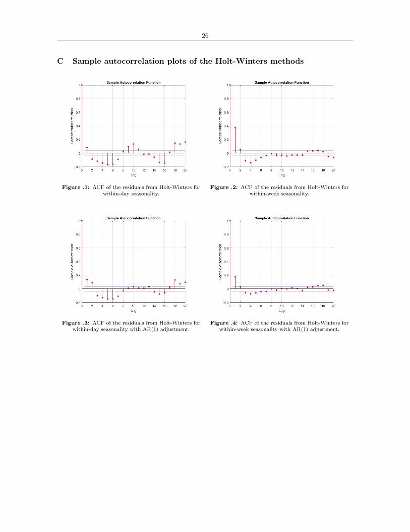
C Sample autocorrelation plots of the Holt-Winters methods

Figure .1: ACF of the residuals from Holt-Winters forwithin-day seasonality.

Figure .2: ACF of the residuals from Holt-Winters forwithin-week seasonality.

Figure .3: ACF of the residuals from Holt-Winters forwithin-day seasonality with AR(1) adjustment.

Figure .4: ACF of the residuals from Holt-Winters forwithin-week seasonality with AR(1) adjustment.

27

D Parameter estimates of model selection procedures

D.1 The MS process with multiplicative seasonality and no adjustment for autocorre-lation.

The MS(2; 48, 336) process without restrictions:

α = 1.000, β = 0.000 and Γ =

[0.489 0.0000.167 0.212

].


α = 1.000, β = 0.000 and Γ =

0.414 0.504 0.2430.372 0.436 0.3050.500 0.500 0.361

.The MS(2; 48, 336) process with restriction 1:

α = 1.000, β = 0.000 and Γ =

[0.336 0.0000.000 0.336

].

The MS(2; 48, 336) process with restriction 2:

α = 1.000, β = 0.000 and Γ =

[0.362 0.3620.362 0.362

].


α = 1.000, β = 0.000 and Γ =

[0.421 0.2580.258 0.421

].

D.2 The MS process with multiplicative seasonality and adjustment for autocorrelation.


α = 0.000, β = 0.000, Γ =

[0.492 0.3710.305 0.383

]and φ = 0.970.


α = 0.000, β = 0.001, Γ =

0.511 0.432 0.3160.383 0.515 0.4280.500 0.500 0.428

and φ = 0.967.


α = 0.000, β = 0.000, Γ =

[0.430 0.0000.000 0.430

]and φ = 0.973.


α = 0.000, β = 0.000, Γ =

[0.350 0.3500.350 0.350

]and φ = 0.963.


α = 0.000, β = 0.000, Γ =

[0.417 0.2650.265 0.417

]and φ = 0.970.

28

D.3 The MS process with additive seasonality and adjustment for autocorrelation.


α = 0.014, β = 0.000, Γ =

[0.522 0.0550.369 0.290

]and φ = 0.980.


α = 0.016, β = 0.001, Γ =

0.521 0.149 0.1320.403 0.780 0.0160.361 0.538 0.523

and φ = 0.978.


α = 0.001, β = 0.000, Γ =

0.614 0.000 0.0000.000 0.614 0.0000.000 0.000 0.614

and φ = 0.979.


α = 0.000, β = 0.000, Γ =

0.387 0.387 0.3870.387 0.387 0.3870.387 0.387 0.387

and φ = 0.992.


α = 0.000, β = 0.000, Γ =

0.554 0.315 0.3150.315 0.554 0.3150.315 0.315 0.554

and φ = 0.985.

29

References

Box, G. E. P., Jenkins, G. M., & Reinsel, G. C. (1993). Time Series Analysis: Forecasting and Control.Prentice Hall, New Jersey.

Chatfield, C. (1987). The Holt-Winters Forecasting Procedure. Journal of the Royal Statistical Society.Series C (Applied Statistics), 27 , 264–279. doi: 10.2307/2347162

Cleveland, R. B., Cleveland, W. S., McRae, J. E., & Terpenning, I. (1990). STL: A Seasonal-TrendDecomposition Procedure Based on Loess. Journal of Official Statistics, 6 , 3–73.

De Livera, A. M., Hyndman, R. J., & Snyder, R. D. (2010). Forecasting Time Series with ComplexSeasonal Patterns using Exponential Smoothing. Department of Econometrics and BusinessStatistics Working Paper Series 15/09 .

Gardner, E. S. (1985). Exponential Smoothing: The State of the Art. International Journal ofForecasting , 4 , 1–28. doi: 10.1002/for.3980040103

Hyndman, R. J., & Athanasopoulos, G. (2012). Forecasting: Principles and Practice. OTexts.Hyndman, R. J., Gould, P. G., Koehler, A. B., Ord, J. K., Snyder, R. D., & Vahid-Araghi, F. (2008).

Forecasting Time Series with Multiple Seasonal Patterns. European Journal of Operational Re-search, 191 , 207–220. doi: 10.1016/j.ejor.2007.08.024

Souza, R. C., Barros, M., & de Miranda, C. V. C. (2007). Short Term Load Forecasting Using DoubleSeasonal Exponential Smoothing and Interventions to Account for Holidays and TemperatureEffects (Tech. Rep.). Pontifıcia Universidade Catolica do Rio de Janeiro.

Taylor, J. W. (2003). Short-Term Electricity Demand Forecasting Using Double Seasonal ExponentialSmoothing. The Journal of the Operational Research Society , 54 , 799–805. doi: 10.1057/palgrave.jors.2601589

Taylor, J. W. (2010). Exponentially Weighted Methods for Forecasting Intra-day Time Series withMultiple Seasonal Cycles . International Journal of Forecasting , 26 , 627–646.

Taylor, J. W. (2012). Short-Term Load Forecasting with Exponentially Weighted Methods. IEEETransactions of Power Systems, 27 , 458–464.

Taylor, J. W., & Buizza, R. (2003). Using Weather Ensemble Predictions in Electricity DemandForecasting . International Journal of Forecasting , 19 , 57–70.

Taylor, J. W., de Menezes, L. M., & McSharry, P. E. (2006). A Comparison of Univariate Methodsfor Forecasting Electricity Demand up to a Day Ahead. International Journal of Forecasting ,22 , 1–16.

using exponential smoothing methods for modelling and ... · using exponential smoothing ......

Documents