EXPONENTIAL SMOOTHING

Exponential smoothing is the most widely used class of procedures for

smoothing discrete time series in order to forecast the immediate future. The

idea of exponential smoothing is to smooth the original series the way the

moving average does and to use the smoothed series in forecasting future

values of the variable of interest. In exponential smoothing, however, we want

to allow the more recent values of the series to have greater influence on the

forecast of future values than the more distant observations.

Exponential smoothing is a simple and pragmatic approach to forecasting,

whereby the forecast is constructed from an exponentially weighted average

of past observations. The largest weight is given to the present observation, less

weight to the immediately preceding observation, even less weight to the

observation before that, and so on (exponential decay of influence of past data)

SIMPLE EXPONENTIAL SMOOTHING

This forecasting method is most widely used of all forecasting techniques. It

requires little computation. This method is used when data pattern is

approximately horizontal (i.e., there is no neither cyclic variation nor

pronounced trend in the historical data).

Let an observed time series be y1, y2, …. yn. Formally, the simple exponential

smoothing equation takes the form of

St+1 = αyt + (1-α) St

Where Si The smoothed value of time series at time i

yi Actual value of time series at time i

α Smoothing constant

In case of simple exponential smoothing, the smoothed statistic is the

Forecasted value.

Ft+1 = αyt + (1-α) Ft

Where Ft+1 Forecasted value of time series at time t+1

Ft Forecasted value of time series at time t

This means:

Ft = αyt-1 + (1-α) Ft-1

Ft-1 = αyt-1 + (1-α) Ft-2

Ft-2 = αyt-2 + (1-α) Ft-3

Ft-3 = αyt-3 + (1-α) Ft-4

Substituting, Ft+1 = αyt + (1-α) Ft = αyt + (1-α)(αyt-1 + (1-α)Ft-1) =

= αyt + α (1-α) yt-1 + (1-α)2 Ft-1 =

= αyt + α (1-α) yt-1 + α (1-α)2 yt-2 + (1-α)3Ft-2

= αyt + α (1-α) yt-1 + α (1-α)2yt-2 + α(1-α)3yt-3 + (1-α)4Ft-3

Generalizing,

Ft+1 = ∑ 𝛼𝑡−1𝑖=0 (1-α)i yt-i + (1-α)t F1

The series of weights used in producing the forecast Ft are α , α (1-α ), α(1-α)2 ,

α(1-α)3…. These weights decline toward zero in an exponential fashion; thus, as

we go back in the series, each value has a smaller weight in terms of its effect

on the forecast. The exponential decline of the weights towards zero is evident.

Choosing α:

After the model is specified, its performance characteristics should be verified

or validated by comparison of its forecast with historical data for the process it

was designed to forecast.

We can use the error measures such as MAPE (Mean absolute percentage error),

MSE (Mean square error) or RMSE (Root mean square error) and α is chosen

such that the error is minimum.

Usually the MSE or RMSE can be used as the criterion for selecting an

appropriate smoothing constant. For instance, by assigning a values from 0.1 to

0.99, we select the value that produces the smallest MSE or RMSE

Since F1 is not known, we can:

Set the first estimate equal to the first observation. Thus we can use 1

Use the average of the first five or six observations for the initial

smoothed value.

DOUBLE EXPONENTIAL SMOOTHIG-HOLT’S TREND METHOD

Under the assumption of no trend in the data, simple exponential smoothing

yields goods results but it fails in case of existence of trend. Double exponential

smoothing is used when there is a linear trend in the data.

The basic idea behind double exponential smoothing is to introduce a term to

take into account the possibility of a series exhibiting some form of trend. This

slope component is itself updated via exponential smoothing.

Suppose the data exhibits a linear trend as:

yt = b0 + b1t + et

where, b0 and b1 may change slowly with time.

The basic equations for Holt’s Method are:

1. µt = αyt + (1 - α) (µt - 1 + T t - 1)

2. Tt = β(µt - µt - 1) + (1 - β )Tt - 1

3. Ft+m = µt + mTt

where

µt Exponentially smoothed value of the series at time t

yt Actual observation of time series at time t

Tt Trend Estimate

αExponential Smoothing Constant for the data

βSmoothing constant for trend

Ft+mm period ahead forecasted value

The difference between 2 successive exponential smoothing values is (µt - µt - 1)

used as an estimate of the trend. The estimate of the trend is smoothed by

multiplying it by β and then multiplying the old estimate of the trend by (1 – β).

To forecast, the trend is multiplied by the number of periods ahead that one

desires to forecast and then the product is added to µt.

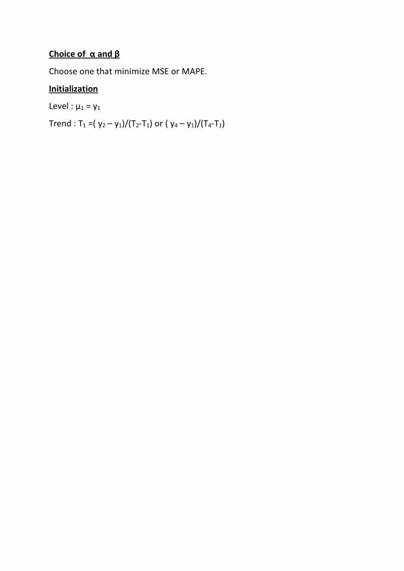
Choice of α and β

Choose one that minimize MSE or MAPE.

Initialization

Level : µ1 = y1

Trend : T1 =( y2 – y1)/(T2-T1) or ( y4 – y1)/(T4-T1)

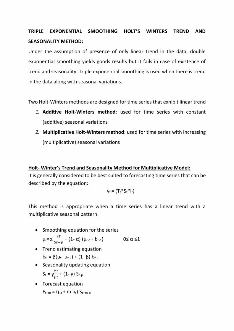
TRIPLE EXPONENTIAL SMOOTHING HOLT’S WINTERS TREND AND

SEASONALITY METHOD:

Under the assumption of presence of only linear trend in the data, double

exponential smoothing yields goods results but it fails in case of existence of

trend and seasonality. Triple exponential smoothing is used when there is trend

in the data along with seasonal variations.

Two Holt-Winters methods are designed for time series that exhibit linear trend

1. Additive Holt-Winters method: used for time series with constant

(additive) seasonal variations

2. Multiplicative Holt-Winters method: used for time series with increasing

(multiplicative) seasonal variations

Holt- Winter’s Trend and Seasonality Method for Multiplicative Model:

It is generally considered to be best suited to forecasting time series that can be

described by the equation:

yt = (Tt*St*It)

This method is appropriate when a time series has a linear trend with a

multiplicative seasonal pattern.

Smoothing equation for the series

µt=α 𝑌𝑡

𝑆𝑡−𝑝 + (1- α) (µt-1+ bt-1) 0≤ α ≤1

Trend estimating equation

bt = β(µt- µt-1) + (1- β) bt-1

Seasonality updating equation

St = γ𝑌𝑡

µt + (1- γ) St-p

Forecast equation

Ft+m = (µt + m bt) St+m-p

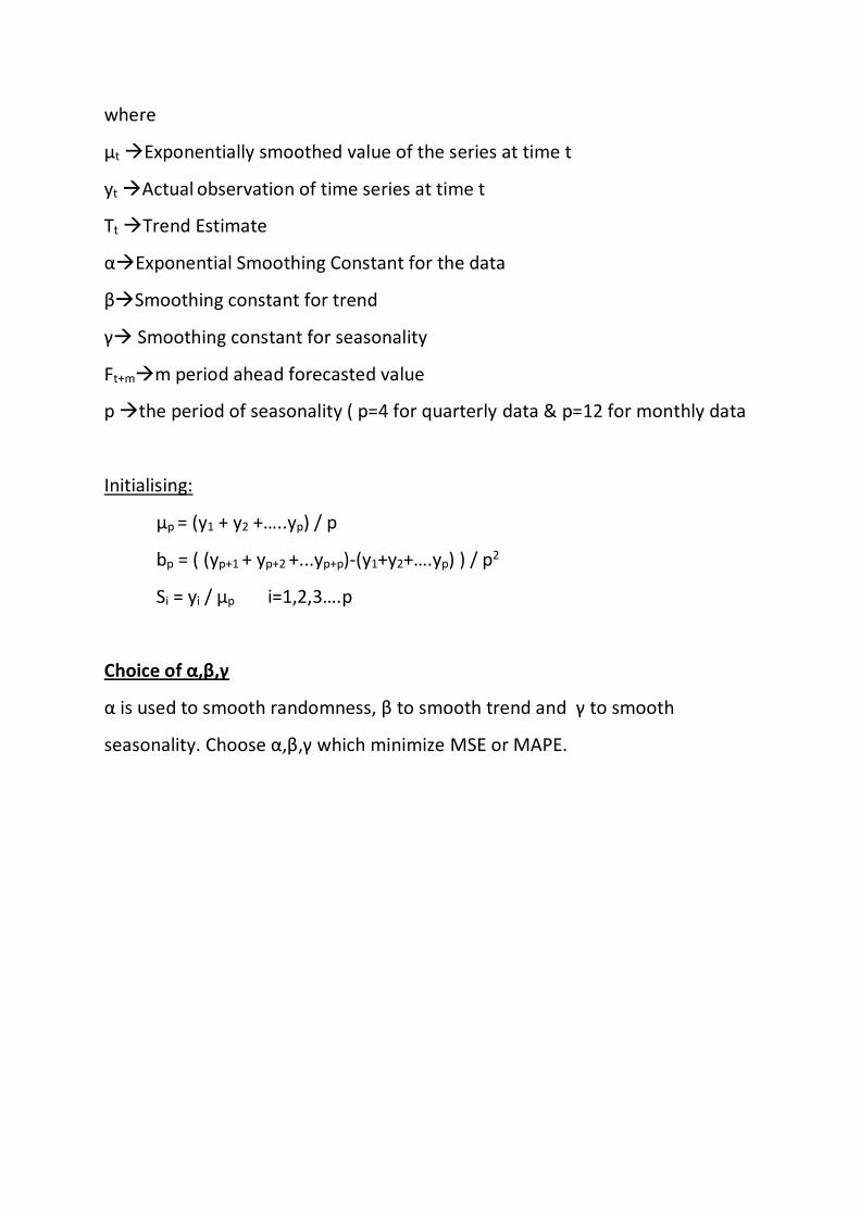
where

µt Exponentially smoothed value of the series at time t

yt Actual observation of time series at time t

Tt Trend Estimate

αExponential Smoothing Constant for the data

βSmoothing constant for trend

γ Smoothing constant for seasonality

Ft+mm period ahead forecasted value

p the period of seasonality ( p=4 for quarterly data & p=12 for monthly data

Initialising:

µp = (y1 + y2 +…..yp) / p

bp = ( (yp+1 + yp+2 +...yp+p)-(y1+y2+….yp) ) / p2

Si = yi / µp i=1,2,3….p

Choice of α,β,γ

α is used to smooth randomness, β to smooth trend and γ to smooth

seasonality. Choose α,β,γ which minimize MSE or MAPE.

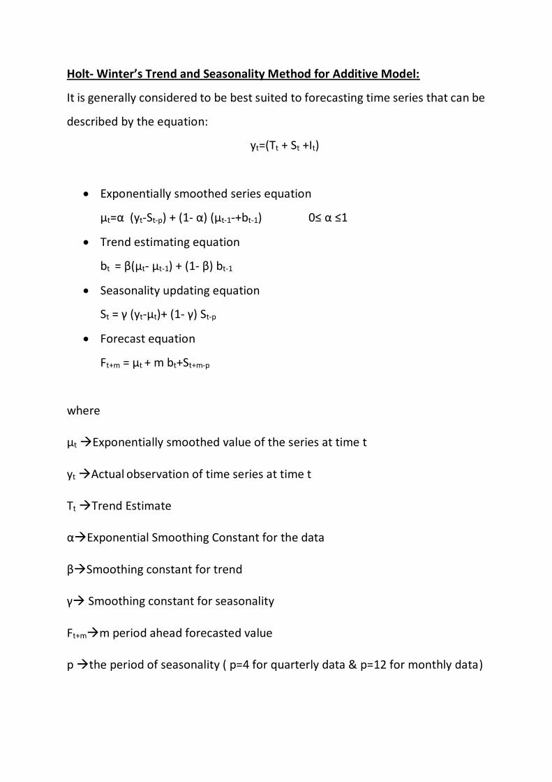
Holt- Winter’s Trend and Seasonality Method for Additive Model:

It is generally considered to be best suited to forecasting time series that can be

described by the equation:

yt=(Tt + St +It)

Exponentially smoothed series equation

µt=α (yt-St-p) + (1- α) (µt-1-+bt-1) 0≤ α ≤1

Trend estimating equation

bt = β(µt- µt-1) + (1- β) bt-1

Seasonality updating equation

St = γ (yt-µt)+ (1- γ) St-p

Forecast equation

Ft+m = µt + m bt+St+m-p

where

µt Exponentially smoothed value of the series at time t

yt Actual observation of time series at time t

Tt Trend Estimate

αExponential Smoothing Constant for the data

βSmoothing constant for trend

γ Smoothing constant for seasonality

Ft+mm period ahead forecasted value

p the period of seasonality ( p=4 for quarterly data & p=12 for monthly data)

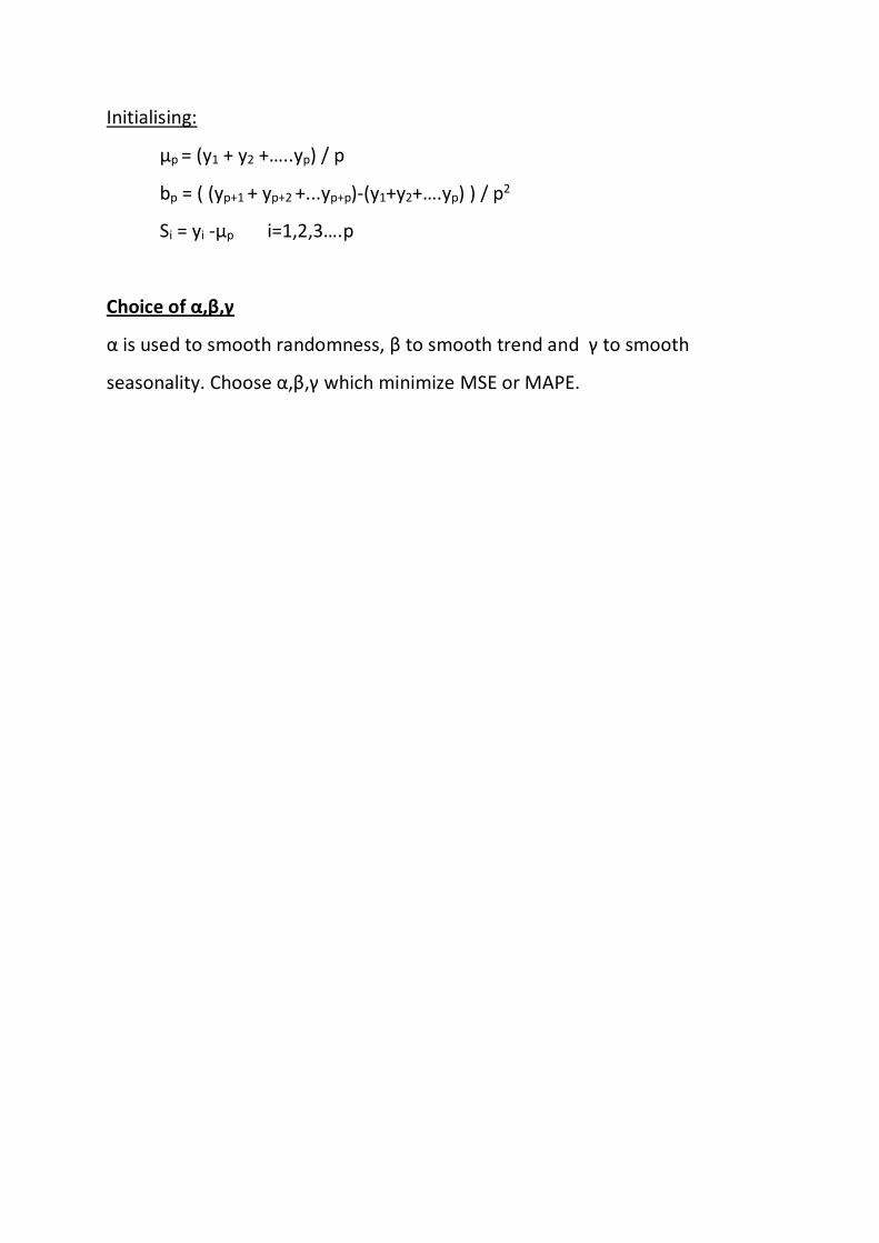
Initialising:

µp = (y1 + y2 +…..yp) / p

bp = ( (yp+1 + yp+2 +...yp+p)-(y1+y2+….yp) ) / p2

Si = yi -µp i=1,2,3….p

Choice of α,β,γ

α is used to smooth randomness, β to smooth trend and γ to smooth

seasonality. Choose α,β,γ which minimize MSE or MAPE.

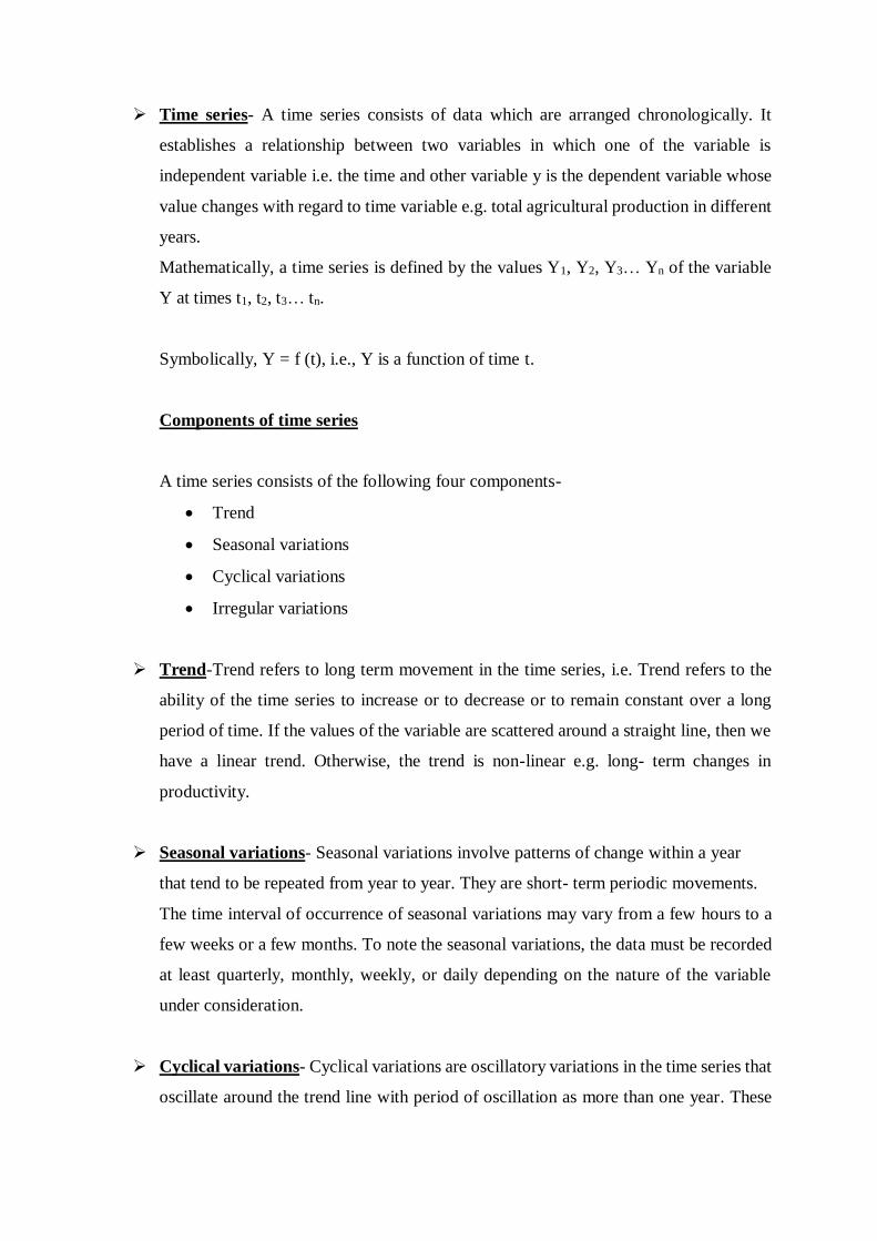
Time series- A time series consists of data which are arranged chronologically. It

establishes a relationship between two variables in which one of the variable is

independent variable i.e. the time and other variable y is the dependent variable whose

value changes with regard to time variable e.g. total agricultural production in different

years.

Mathematically, a time series is defined by the values Y1, Y2, Y3… Yn of the variable

Y at times t1, t2, t3… tn.

Symbolically, Y = f (t), i.e., Y is a function of time t.

Components of time series

A time series consists of the following four components-

Trend

Seasonal variations

Cyclical variations

Irregular variations

Trend-Trend refers to long term movement in the time series, i.e. Trend refers to the

ability of the time series to increase or to decrease or to remain constant over a long

period of time. If the values of the variable are scattered around a straight line, then we

have a linear trend. Otherwise, the trend is non-linear e.g. long- term changes in

productivity.

Seasonal variations- Seasonal variations involve patterns of change within a year

that tend to be repeated from year to year. They are short- term periodic movements.

The time interval of occurrence of seasonal variations may vary from a few hours to a

few weeks or a few months. To note the seasonal variations, the data must be recorded

at least quarterly, monthly, weekly, or daily depending on the nature of the variable

under consideration.

Cyclical variations- Cyclical variations are oscillatory variations in the time series that

oscillate around the trend line with period of oscillation as more than one year. These

variations do not follow any regular pattern and move in somewhat unpredictable

manner. These are upswings and downswings in the time series that are observable over

extended periods of time.

Irregular variations- The irregular component of the time series is the residual factor

that accounts for the deviations of the actual time series values from what we would

expect from the trend, seasonal, and cyclical components. It accounts for the random

availability in the time series. The irregular component is caused by the short-term,

unanticipated, and non-recurring factors that affect the time series, viz. earthquakes,

floods etc.

MODELS OF DECOMPOSITION

There are two models of decomposition of time series:

The additive model- This model is used when it is assumed that the four

components are independent of one another, i.e., when the pattern of occurrence

and the magnitude of movement in any particular component are not affected

by other components under this assumption, the magnitude of time series (Y(t)),

at any time t is the sum of the separate influences of its four components, i.e.

Y(t)= T(t) + S(t)+ C(t)+ I(t)

where T(t)= Trend variations

S(t)= seasonal variations

C(t)= cyclical variations

I(t)= irregular variations

Multiplicative model-This model is used when it is assumed that the

components may depend on each other.

Y(t)= T(t)*S(t)*C(t)*I(t)

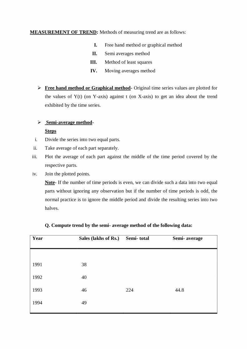
MEASUREMENT OF TREND: Methods of measuring trend are as follows:

I. Free hand method or graphical method

II. Semi averages method

III. Method of least squares

IV. Moving averages method

Free hand method or Graphical method- Original time series values are plotted for

the values of Y(t) (on Y-axis) against t (on X-axis) to get an idea about the trend

exhibited by the time series.

Semi-average method-

Steps

i. Divide the series into two equal parts.

ii. Take average of each part separately.

iii. Plot the average of each part against the middle of the time period covered by the

respective parts.

iv. Join the plotted points.

Note- If the number of time periods is even, we can divide such a data into two equal

parts without ignoring any observation but if the number of time periods is odd, the

normal practice is to ignore the middle period and divide the resulting series into two

halves.

Q. Compute trend by the semi- average method of the following data:

Year Sales (lakhs of Rs.) Semi- total Semi- average

1991 38

1992 40

1993 46 224 44.8

1994 49

1995 51

1996 55

1997 61

1998 63

1999 69 345 69.0

2000 72

2001 80

These two semi- averages are plotted in the middle of the respective time spans. Thus 44.8

is plotted against 1993; and 69.0 against 1999. These two points are then connected by a

straight line.

Method of least squares

i. Fitting a straight line(Line of best fit)-

The equation of straight line is of the form Y= a+bX

By the method of least squares, the normal equations to find the values of

a and b are

∑Y=na+b∑X

∑XY=a∑X+b∑(X^2)

Q. The following are the annual profits in thousands in a certain business. By the method

of least squares fit a straight line.

Year Profits(000) t-1994

(X)

XY X^2 Y_cap

1991 60 -3 -180 9

1992 72 -2 -144 4

1993 75 -1 -75 1

1994 65 0 0 0 Y_cap=76+4.857*X

1995 80 1 80 1

1996 85 2 170 4

1997 95 3 285 9

N=7 ∑Y ∑X=0 ∑XY= ∑X^2=

=532 136 28

The equation of straight line trend is Y_cap= a+b*X

By the method of least squares

a=∑Y/N= 76

b=∑X*Y/∑X^2=4.857

The trend equation would be Y_cap= 76+ 4.857*X

ii. Fitting a quadratic trend-

Y=a+bX+cX^2

In this case, the normal equations by the method of least squares are

∑Y=na+b∑X+c∑(X^2)

∑XY=a∑X+b∑(X^2)+c∑(X^3)

∑X^2*Y=a∑(X^2)+b∑(X^3)+c∑(X^4)

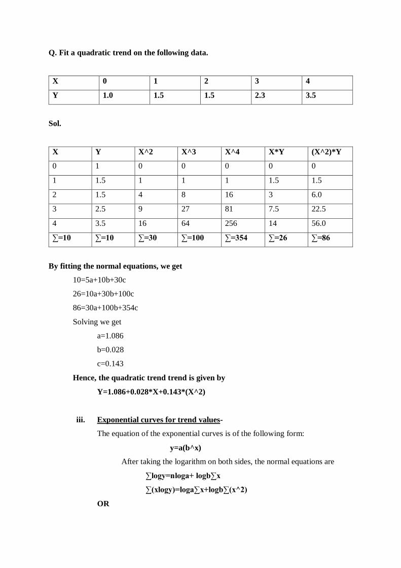
Q. Fit a quadratic trend on the following data.

X 0 1 2 3 4

Y 1.0 1.5 1.5 2.3 3.5

Sol.

X Y X^2 X^3 X^4 X*Y (X^2)*Y

0 1 0 0 0 0 0

1 1.5 1 1 1 1.5 1.5

2 1.5 4 8 16 3 6.0

3 2.5 9 27 81 7.5 22.5

4 3.5 16 64 256 14 56.0

∑=10 ∑=10 ∑=30 ∑=100 ∑=354 ∑=26 ∑=86

By fitting the normal equations, we get

10=5a+10b+30c

26=10a+30b+100c

86=30a+100b+354c

Solving we get

a=1.086

b=0.028

c=0.143

Hence, the quadratic trend trend is given by

Y=1.086+0.028*X+0.143*(X^2)

iii. Exponential curves for trend values-

The equation of the exponential curves is of the following form:

y=a(b^x)

After taking the logarithm on both sides, the normal equations are

∑logy=nloga+ logb∑x

∑(xlogy)=loga∑x+logb∑(x^2)

OR

∑Y=nA+B∑x

∑(xY)=A∑x+B∑(x^2)

Where, A = log a and B = log b

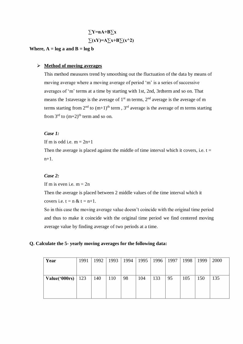
Method of moving averages

This method measures trend by smoothing out the fluctuation of the data by means of

moving average where a moving average of period ‘m’ is a series of successive

averages of ‘m’ terms at a time by starting with 1st, 2nd, 3rdterm and so on. That

means the 1staverage is the average of 1st m terms, 2nd average is the average of m

terms starting from 2nd to (m+1)th term , 3rd average is the average of m terms starting

from 3rd to (m+2)th term and so on.

Case 1:

If m is odd i.e. m = 2n+1

Then the average is placed against the middle of time interval which it covers, i.e. t =

n+1.

Case 2:

If m is even i.e. m = 2n

Then the average is placed between 2 middle values of the time interval which it

covers i.e. t = n & t = n+1.

So in this case the moving average value doesn’t coincide with the original time period

and thus to make it coincide with the original time period we find centered moving

average value by finding average of two periods at a time.

Q. Calculate the 5- yearly moving averages for the following data:

Year 1991 1992 1993 1994 1995 1996 1997 1998 1999 2000

Value(‘000rs) 123 140 110 98 104 133 95 105 150 135

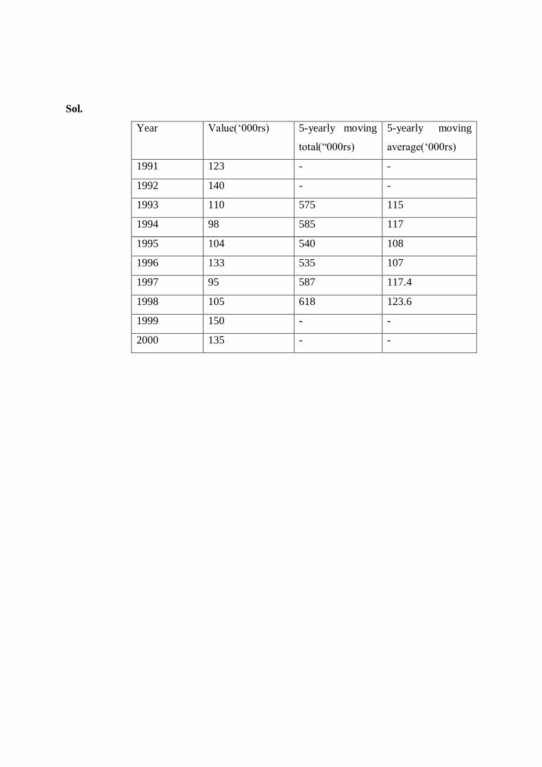
Sol.

Year Value(‘000rs) 5-yearly moving

total(“000rs)

5-yearly moving

average(‘000rs)

1991 123 - -

1992 140 - -

1993 110 575 115

1994 98 585 117

1995 104 540 108

1996 133 535 107

1997 95 587 117.4

1998 105 618 123.6

1999 150 - -

2000 135 - -

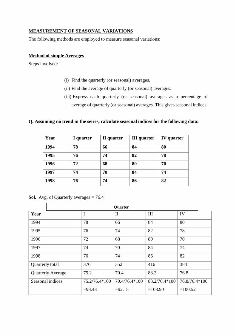
MEASUREMENT OF SEASONAL VARIATIONS

The following methods are employed to measure seasonal variations:

Method of simple Averages

Steps involved:

(i) Find the quarterly (or seasonal) averages.

(ii) Find the average of quarterly (or seasonal) averages.

(iii) Express each quarterly (or seasonal) averages as a percentage of

average of quarterly (or seasonal) averages. This gives seasonal indices.

Q. Assuming no trend in the series, calculate seasonal indices for the following data:

Year I quarter II quarter III quarter IV quarter

1994 78 66 84 80

1995 76 74 82 78

1996 72 68 80 70

1997 74 70 84 74

1998 76 74 86 82

Sol. Avg. of Quarterly averages = 76.4

Year I II III IV

1994 78 66 84 80

1995 76 74 82 78

1996 72 68 80 70

1997 74 70 84 74

1998 76 74 86 82

Quarterly total 376 352 416 384

Quarterly Average 75.2 70.4 83.2 76.8

Seasonal indices 75.2/76.4*100

=98.43

70.4/76.4*100

=92.15

83.2/76.4*100

=108.90

76.8/76.4*100

=100.52

Quarter

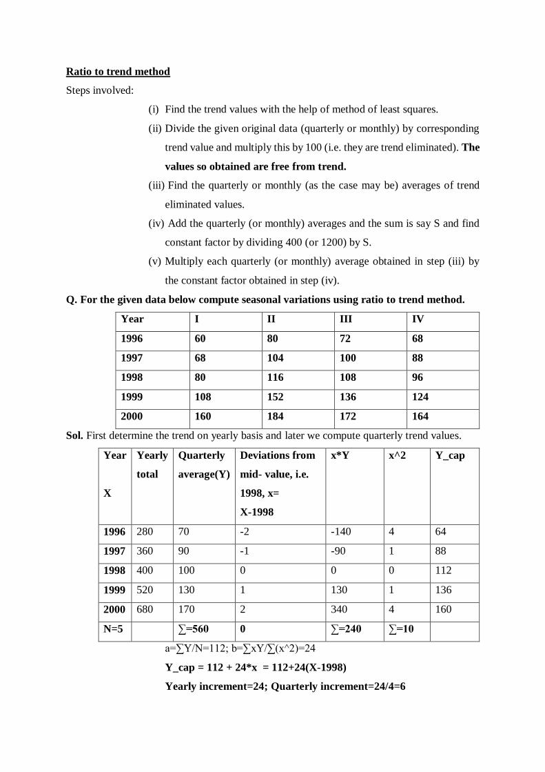
Ratio to trend method

Steps involved:

(i) Find the trend values with the help of method of least squares.

(ii) Divide the given original data (quarterly or monthly) by corresponding

trend value and multiply this by 100 (i.e. they are trend eliminated). The

values so obtained are free from trend.

(iii) Find the quarterly or monthly (as the case may be) averages of trend

eliminated values.

(iv) Add the quarterly (or monthly) averages and the sum is say S and find

constant factor by dividing 400 (or 1200) by S.

(v) Multiply each quarterly (or monthly) average obtained in step (iii) by

the constant factor obtained in step (iv).

Q. For the given data below compute seasonal variations using ratio to trend method.

Year I II III IV

1996 60 80 72 68

1997 68 104 100 88

1998 80 116 108 96

1999 108 152 136 124

2000 160 184 172 164

Sol. First determine the trend on yearly basis and later we compute quarterly trend values.

Year

X

Yearly

total

Quarterly

average(Y)

Deviations from

mid- value, i.e.

1998, x=

X-1998

x*Y x^2 Y_cap

1996 280 70 -2 -140 4 64

1997 360 90 -1 -90 1 88

1998 400 100 0 0 0 112

1999 520 130 1 130 1 136

2000 680 170 2 340 4 160

N=5 ∑=560 0 ∑=240 ∑=10

a=∑Y/N=112; b=∑xY/∑(x^2)=24

Y_cap = 112 + 24*x = 112+24(X-1998)

Yearly increment=24; Quarterly increment=24/4=6

Calculation of quarterly trend values:

Consider 1996, trend value for middle quarter, i.e. half of 2nd and half of 3rd is 64. Quarterly

increment is 6. So the trend value of 2nd quarter is 64-6/2=61 and for 3rd quarter is 64+6/2=67.

Trend value for the first quarter is 61-6=55 and of the 4th quarter is 67+6=73.

Quarterly trend values

Year I II III IV

1996 55 61 67 73

1997 79 85 91 97

1998 103 109 115 121

1999 127 133 139 145

2000 151 157 163 169

The given values of the time series will now be expressed as percentages of the

corresponding trend values given above. These are trend eliminated values.

Trend eliminated values

Year I II III IV

1996 109.09 131.15 107.46 93.15

1997 86.08 122.35 109.89 90.72

1998 77.67 106.42 93.91 79.34

1999 85.04 114.29 97.84 85.52

2000 105.96 117.20 105.52 97.04

Total 463.84 591.41 514.62 445.77

Quarterly

average

92.77 118.28 102.92 89.15

Seasonal

Indices

92.05 117.36 102.12 84.47

60/55*100=109.09, 80/61*100=131.15, etc.

Sum of the quarterly averages= 403.12

Constant factor=400/403.12=0.99226

Seasonal index for the first quarter=92.77*0.992226=92.05

Seasonal index for the second quarter=118.28*0.992226=117.36, and so on.

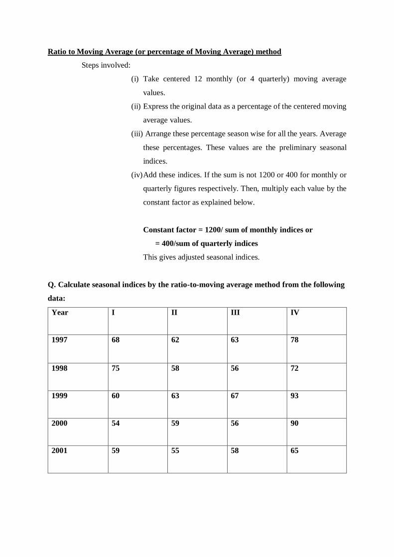
Ratio to Moving Average (or percentage of Moving Average) method

Steps involved:

(i) Take centered 12 monthly (or 4 quarterly) moving average

values.

(ii) Express the original data as a percentage of the centered moving

average values.

(iii) Arrange these percentage season wise for all the years. Average

these percentages. These values are the preliminary seasonal

indices.

(iv) Add these indices. If the sum is not 1200 or 400 for monthly or

quarterly figures respectively. Then, multiply each value by the

constant factor as explained below.

Constant factor = 1200/ sum of monthly indices or

= 400/sum of quarterly indices

This gives adjusted seasonal indices.

Q. Calculate seasonal indices by the ratio-to-moving average method from the following

data:

Year I II III IV

1997 68 62 63 78

1998 75 58 56 72

1999 60 63 67 93

2000 54 59 56 90

2001 59 55 58 65

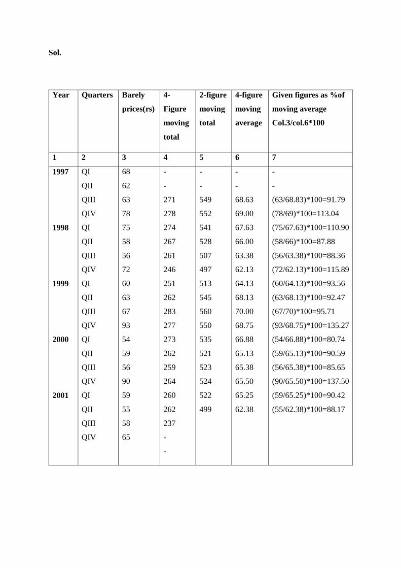
Sol.

Year Quarters Barely

prices(rs)

4-

Figure

moving

total

2-figure

moving

total

4-figure

moving

average

Given figures as %of

moving average

Col.3/col.6*100

1 2 3 4 5 6 7

1997

1998

1999

2000

2001

QI

QII

QIII

QIV

QI

QII

QIII

QIV

QI

QII

QIII

QIV

QI

QII

QIII

QIV

QI

QII

QIII

QIV

68

62

63

78

75

58

56

72

60

63

67

93

54

59

56

90

59

55

58

65

-

-

271

278

274

267

261

246

251

262

283

277

273

262

259

264

260

262

237

-

-

-

-

549

552

541

528

507

497

513

545

560

550

535

521

523

524

522

499

-

-

68.63

69.00

67.63

66.00

63.38

62.13

64.13

68.13

70.00

68.75

66.88

65.13

65.38

65.50

65.25

62.38

-

-

(63/68.83)*100=91.79

(78/69)*100=113.04

(75/67.63)*100=110.90

(58/66)*100=87.88

(56/63.38)*100=88.36

(72/62.13)*100=115.89

(60/64.13)*100=93.56

(63/68.13)*100=92.47

(67/70)*100=95.71

(93/68.75)*100=135.27

(54/66.88)*100=80.74

(59/65.13)*100=90.59

(56/65.38)*100=85.65

(90/65.50)*100=137.50

(59/65.25)*100=90.42

(55/62.38)*100=88.17

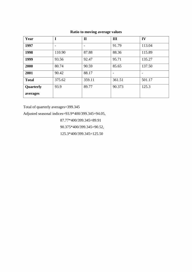
Ratio to moving average values

Year I II III IV

1997 - - 91.79 113.04

1998 110.90 87.88 88.36 115.89

1999 93.56 92.47 95.71 135.27

2000 80.74 90.59 85.65 137.50

2001 90.42 88.17 - -

Total 375.62 359.11 361.51 501.17

Quarterly

averages

93.9 89.77 90.373 125.3

Total of quarterly averages=399.345

Adjusted seasonal indices=93.9*400/399.345=94.05,

87.77*400/399.345=89.91

90.375*400/399.345=90.52,

125.3*400/399.345=125.50

Measurement of Cyclical Variation

We know that a time series consisting of annual data for longer periods is depicted by trend lines. This

facilitates us to isolate the component of secular trend variation from the series and examine it for

cyclical, seasonal and irregular components. Here, we will look at "Residual Method", by which one

can isolate the cyclical variation component. This method can be bifurcated into two measures:

Percent of Trend method

Relative Cyclical Residual method.

Both these measures are expressed in terms of percentage. We look at each of them.

1. Percent of Trend Method:

When the ratio of actual values (Y) and the corresponding estimated trend values ( Ŷ ) is multiplied by

100, we are expressing the cyclical variation component as a percent of trend. Mathematically, we

express it as

(Y/ Ŷ ) * 100

2. Relative Cyclical Residual Method:

In this measure, we take the ratio of the difference between the Y and the corresponding Ŷ values (that

is, Y - Ŷ ), and the Ŷ values. To express these values in terms of percentage we multiply them by 100.

In other words, the percentage deviation from the trend is found for all the values in the series.

Mathematically, this is expressed as:

[ (Y- Ŷ)/ Ŷ ] * 100

Example:

Year (t) Y Yₑ (Y/Yₑ)*100 Y-Yₑ ((Y-Yₑ)/Yₑ)*100

1989 77 83 92.77 -6 -7.22

1990 88 85 103.52 3 3.52

1991 94 87 108.04 7 8.04

1992 85 89 95.50 -4 -4.49

1993 91 91 100.00 0 0

1994 98 93 105.37 5 5.37

1995 90 95 94.73 -5 -5.26

In 1989, the percentage of trend indicates that the actual sales were 92.77% of the expected sales for

that year.

For the same year, the relative cyclical residual indicates that the actual sales were 7.22% short of the

expected value.

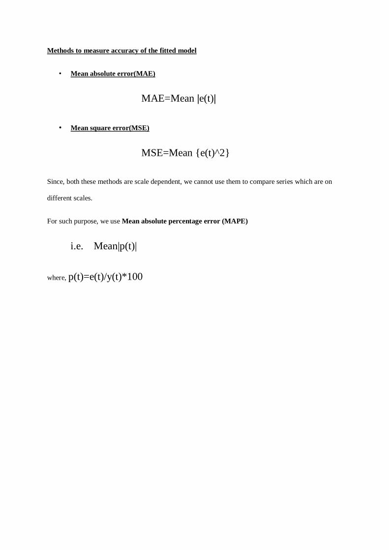
Methods to measure accuracy of the fitted model

• Mean absolute error(MAE)

MAE=Mean |e(t)|

• Mean square error(MSE)

MSE=Mean {e(t)^2}

Since, both these methods are scale dependent, we cannot use them to compare series which are on

different scales.

For such purpose, we use Mean absolute percentage error (MAPE)

i.e. Mean|p(t)|

where, p(t)=e(t)/y(t)*100

STATIONARY RANDOM SERIES

A strictly stationary stochastic process is one where given t1, . . ., tn; the joint

statistical distribution of Xt1 , . . ., Xtn is the same as the joint statistical

distribution of Xt1+τ, . . ., Xtℓ+τ for all ℓ and τ .

This is an extremely strong definition: it means that all moments of all degrees

(expectations, variances, third order and higher) of the process, anywhere are

the same. It also means that the joint distribution of (Xt , Xs) is the same as (Xt+r,

Xs+r) and hence cannot depend on s or t but only on the distance between s and

t, i.e. s − t.

Since the definition of strict stationarity is generally too strict for everyday life

a weaker definition of second order or weak stationarity is usually used.

Weak Stationarity or Covariance Stationarity means that mean and the

variance of a stochastic process do not depend on t (that is they are constant)

and the autocovariance between Xt and Xt+τ only can depend on the lag τ (τ is an

integer, the quantities also need to be finite). Hence for stationary processes,

{Xt}, the definition of autocovariance is

γ(τ ) = cov(Xt , Xt+τ ), for integers τ .

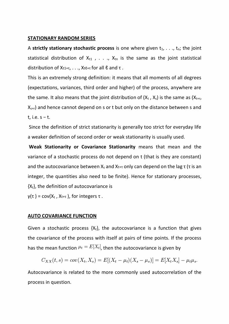
AUTO COVARIANCE FUNCTION

Given a stochastic process {Xt}, the autocovariance is a function that gives

the covariance of the process with itself at pairs of time points. If the process

has the mean function , then the autocovariance is given by

Autocovariance is related to the more commonly used autocorrelation of the

process in question.

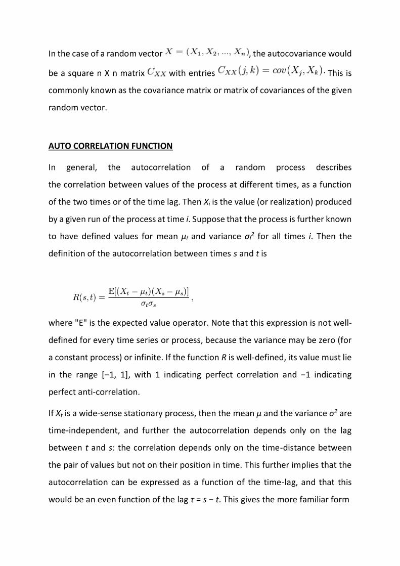
In the case of a random vector , the autocovariance would

be a square n X n matrix with entries This is

commonly known as the covariance matrix or matrix of covariances of the given

random vector.

AUTO CORRELATION FUNCTION

In general, the autocorrelation of a random process describes

the correlation between values of the process at different times, as a function

of the two times or of the time lag. Then Xi is the value (or realization) produced

by a given run of the process at time i. Suppose that the process is further known

to have defined values for mean μi and variance σi2 for all times i. Then the

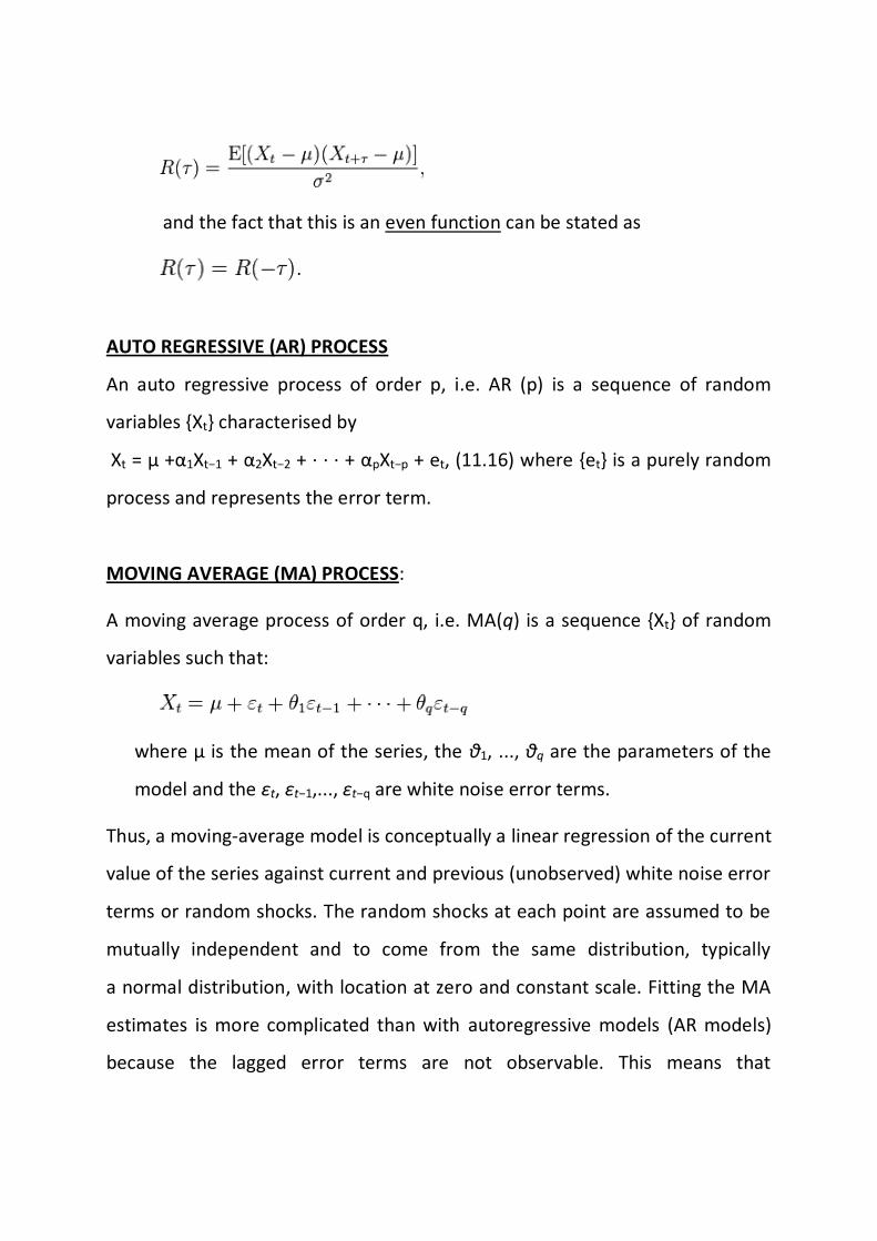
definition of the autocorrelation between times s and t is

where "E" is the expected value operator. Note that this expression is not well-

defined for every time series or process, because the variance may be zero (for

a constant process) or infinite. If the function R is well-defined, its value must lie

in the range [−1, 1], with 1 indicating perfect correlation and −1 indicating

perfect anti-correlation.

If Xt is a wide-sense stationary process, then the mean μ and the variance σ2 are

time-independent, and further the autocorrelation depends only on the lag

between t and s: the correlation depends only on the time-distance between

the pair of values but not on their position in time. This further implies that the

autocorrelation can be expressed as a function of the time-lag, and that this

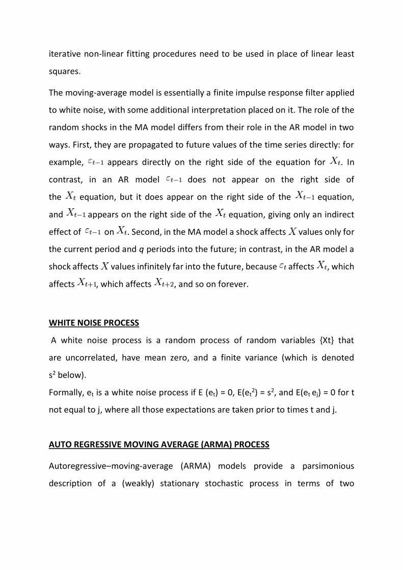
would be an even function of the lag τ = s − t. This gives the more familiar form

and the fact that this is an even function can be stated as

AUTO REGRESSIVE (AR) PROCESS

An auto regressive process of order p, i.e. AR (p) is a sequence of random

variables {Xt} characterised by

Xt = µ +α1Xt−1 + α2Xt−2 + · · · + αpXt−p + et, (11.16) where {et} is a purely random

process and represents the error term.

MOVING AVERAGE (MA) PROCESS:

A moving average process of order q, i.e. MA(q) is a sequence {Xt} of random

variables such that:

where μ is the mean of the series, the θ1, ..., θq are the parameters of the

model and the εt, εt−1,..., εt−q are white noise error terms.

Thus, a moving-average model is conceptually a linear regression of the current

value of the series against current and previous (unobserved) white noise error

terms or random shocks. The random shocks at each point are assumed to be

mutually independent and to come from the same distribution, typically

a normal distribution, with location at zero and constant scale. Fitting the MA

estimates is more complicated than with autoregressive models (AR models)

because the lagged error terms are not observable. This means that

iterative non-linear fitting procedures need to be used in place of linear least

squares.

The moving-average model is essentially a finite impulse response filter applied

to white noise, with some additional interpretation placed on it. The role of the

random shocks in the MA model differs from their role in the AR model in two

ways. First, they are propagated to future values of the time series directly: for

example, appears directly on the right side of the equation for . In

contrast, in an AR model does not appear on the right side of

the equation, but it does appear on the right side of the equation,

and appears on the right side of the equation, giving only an indirect

effect of on . Second, in the MA model a shock affects values only for

the current period and q periods into the future; in contrast, in the AR model a

shock affects values infinitely far into the future, because affects , which

affects , which affects , and so on forever.

WHITE NOISE PROCESS

A white noise process is a random process of random variables {Xt} that

are uncorrelated, have mean zero, and a finite variance (which is denoted

s2 below).

Formally, et is a white noise process if E (et) = 0, E(et2) = s2, and E(et ej) = 0 for t

not equal to j, where all those expectations are taken prior to times t and j.

AUTO REGRESSIVE MOVING AVERAGE (ARMA) PROCESS

Autoregressive–moving-average (ARMA) models provide a parsimonious

description of a (weakly) stationary stochastic process in terms of two

polynomials, one for the auto-regression and the second for the moving

average.

Given a time series of data Xt, the ARMA model is a tool for understanding and,

perhaps, predicting future values in this series. The model consists of two parts,

an autoregressive (AR) part and a moving average (MA) part. The model is

usually then referred to as the ARMA (p, q) model where p is the order of the

autoregressive part and q is the order of the moving average part

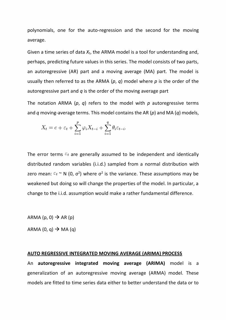
The notation ARMA (p, q) refers to the model with p autoregressive terms

and q moving-average terms. This model contains the AR (p) and MA (q) models,

The error terms are generally assumed to be independent and identically

distributed random variables (i.i.d.) sampled from a normal distribution with

zero mean: ~ N (0, σ2) where σ2 is the variance. These assumptions may be

weakened but doing so will change the properties of the model. In particular, a

change to the i.i.d. assumption would make a rather fundamental difference.

ARMA (p, 0) AR (p)

ARMA (0, q) MA (q)

AUTO REGRESSIVE INTEGRATED MOVING AVERAGE (ARIMA) PROCESS

An autoregressive integrated moving average (ARIMA) model is a

generalization of an autoregressive moving average (ARMA) model. These

models are fitted to time series data either to better understand the data or to

predict future points in the series (forecasting). They are applied in some cases

where data show evidence of non-stationarity, i.e. when the mean & variance

of some of the time series may be time variant.