oracle® retail demand forecasting · pdf filestandard exponential smoothing ... time...
TRANSCRIPT

Oracle® Retail Demand ForecastingUser Guide for the RPAS Classic Client
Release 13.2.3
E40291-02
April 2013

Oracle Retail Demand Forecasting User Guide for the RPAS Classic Client, 13.2.3
E40291-02
Copyright © 2013, Oracle and/or its affiliates. All rights reserved.
Primary Author: Melissa Artley
This software and related documentation are provided under a license agreement containing restrictions on use and disclosure and are protected by intellectual property laws. Except as expressly permitted in your license agreement or allowed by law, you may not use, copy, reproduce, translate, broadcast, modify, license, transmit, distribute, exhibit, perform, publish, or display any part, in any form, or by any means. Reverse engineering, disassembly, or decompilation of this software, unless required by law for interoperability, is prohibited.
The information contained herein is subject to change without notice and is not warranted to be error-free. If you find any errors, please report them to us in writing.
If this is software or related documentation that is delivered to the U.S. Government or anyone licensing it on behalf of the U.S. Government, the following notice is applicable:
U.S. GOVERNMENT END USERS: Oracle programs, including any operating system, integrated software, any programs installed on the hardware, and/or documentation, delivered to U.S. Government end users are "commercial computer software" pursuant to the applicable Federal Acquisition Regulation and agency-specific supplemental regulations. As such, use, duplication, disclosure, modification, and adaptation of the programs, including any operating system, integrated software, any programs installed on the hardware, and/or documentation, shall be subject to license terms and license restrictions applicable to the programs. No other rights are granted to the U.S. Government.
This software or hardware is developed for general use in a variety of information management applications. It is not developed or intended for use in any inherently dangerous applications, including applications that may create a risk of personal injury. If you use this software or hardware in dangerous applications, then you shall be responsible to take all appropriate fail-safe, backup, redundancy, and other measures to ensure its safe use. Oracle Corporation and its affiliates disclaim any liability for any damages caused by use of this software or hardware in dangerous applications.
Oracle is a registered trademark of Oracle Corporation and/or its affiliates. Other names may be trademarks of their respective owners.
This software or hardware and documentation may provide access to or information on content, products, and services from third parties. Oracle Corporation and its affiliates are not responsible for and expressly disclaim all warranties of any kind with respect to third-party content, products, and services. Oracle Corporation and its affiliates will not be responsible for any loss, costs, or damages incurred due to your access to or use of third-party content, products, or services.
Licensing Note: This media pack includes a Restricted Use license for Oracle Retail Predictive Application Server (RPAS) - Enterprise Engine to support Oracle® Retail Demand Forecasting only.
Value-Added Reseller (VAR) Language
Oracle Retail VAR Applications
The following restrictions and provisions only apply to the programs referred to in this section and licensed to you. You acknowledge that the programs may contain third party software (VAR applications) licensed to Oracle. Depending upon your product and its version number, the VAR applications may include:
(i) the MicroStrategy Components developed and licensed by MicroStrategy Services Corporation (MicroStrategy) of McLean, Virginia to Oracle and imbedded in the MicroStrategy for Oracle Retail Data Warehouse and MicroStrategy for Oracle Retail Planning & Optimization applications.
(ii) the Wavelink component developed and licensed by Wavelink Corporation (Wavelink) of Kirkland, Washington, to Oracle and imbedded in Oracle Retail Mobile Store Inventory Management.
(iii) the software component known as Access Via™ licensed by Access Via of Seattle, Washington, and imbedded in Oracle Retail Signs and Oracle Retail Labels and Tags.
(iv) the software component known as Adobe Flex™ licensed by Adobe Systems Incorporated of San Jose, California, and imbedded in Oracle Retail Promotion Planning & Optimization application.
You acknowledge and confirm that Oracle grants you use of only the object code of the VAR Applications. Oracle will not deliver source code to the VAR Applications to you. Notwithstanding any other term or condition of the agreement and this ordering document, you shall not cause or permit alteration of any VAR Applications. For purposes of this section, “alteration” refers to all alterations, translations, upgrades, enhancements, customizations or modifications of all or any portion of the VAR Applications including all reconfigurations, reassembly or reverse assembly, re-engineering or reverse engineering and recompilations or reverse compilations of the VAR Applications or any derivatives of the VAR Applications. You acknowledge that it shall be a breach of the agreement to utilize the relationship, and/or confidential information of the VAR Applications for purposes of competitive discovery.

The VAR Applications contain trade secrets of Oracle and Oracle's licensors and Customer shall not attempt, cause, or permit the alteration, decompilation, reverse engineering, disassembly or other reduction of the VAR Applications to a human perceivable form. Oracle reserves the right to replace, with functional equivalent software, any of the VAR Applications in future releases of the applicable program.


v
Contents
Send Us Your Comments ...................................................................................................................... xvii
Preface ............................................................................................................................................................... xix
1 Introduction
Forecasting Challenges and RDF Solutions........................................................................................ 1-1Selecting the Best Forecasting Method............................................................................................ 1-2Overcoming Data Sparsity Through Source Level Forecasting .................................................. 1-2Forecasting Demand for New Products and Locations................................................................ 1-3Managing Forecasting Results Through Automated Exception Reporting .............................. 1-3Incorporating the Effects of Promotions and Other Event-Based Challenges on Demand .... 1-3
Oracle Retail Demand Forecasting Architecture................................................................................ 1-4The Oracle Retail Predictive Application Server and RDF .......................................................... 1-4Global Domain Versus Simple Domain Environment ................................................................. 1-4
Oracle Retail Demand Forecasting Workbook Template Groups .................................................. 1-5Forecast ................................................................................................................................................ 1-6Promote (Promotional Forecasting) ................................................................................................ 1-6Curve.................................................................................................................................................... 1-7
RDF Solution and Business Process Overview .................................................................................. 1-7RDF and the Oracle Retail Enterprise ............................................................................................. 1-7RDF Primary Workflow .................................................................................................................... 1-8
2 Preprocessing
Preprocessing Methods ........................................................................................................................... 2-2Standard Median................................................................................................................................ 2-2Retail Median...................................................................................................................................... 2-3Standard Exponential Smoothing.................................................................................................... 2-3Lost Sales Standard Exponential Smoothing ................................................................................. 2-5Override............................................................................................................................................... 2-6Increment............................................................................................................................................. 2-7Forecast Sigma.................................................................................................................................... 2-7Forecast Sigma Event......................................................................................................................... 2-8Clear ..................................................................................................................................................... 2-8No Filtering ......................................................................................................................................... 2-8
Preprocessing for Stock-outs.................................................................................................................. 2-8

vi
Preprocessing for Promotional Forecasting ........................................................................................ 2-8
3 Oracle Retail Demand Forecasting Methods
Forecasting Techniques Used in RDF................................................................................................... 3-1Exponential Smoothing ..................................................................................................................... 3-1Regression Analysis ........................................................................................................................... 3-1Bayesian Analysis............................................................................................................................... 3-2Prediction Intervals............................................................................................................................ 3-2Automatic Method Selection ............................................................................................................ 3-2Source Level Forecasting................................................................................................................... 3-2Promotional Forecasting ................................................................................................................... 3-2
Time Series (Statistical) Forecasting Methods.................................................................................... 3-2Why Use Statistical Forecasting? ..................................................................................................... 3-3Exponential Smoothing (ES) Forecasting Methods....................................................................... 3-4Average................................................................................................................................................ 3-4Simple Exponential Smoothing........................................................................................................ 3-5Croston's Method ............................................................................................................................... 3-5Simple/Intermittent Exponential Smoothing ................................................................................ 3-6Holt Exponential Smoothing ............................................................................................................ 3-6Multiplicative Winters Exponential Smoothing ............................................................................ 3-7
Oracle Winters............................................................................................................................. 3-8Oracle Winters Decomposition ................................................................................................. 3-8Winters Standard ........................................................................................................................ 3-9Winters Responsive .................................................................................................................... 3-9
Additive Winters Exponential Smoothing .................................................................................. 3-10Seasonal Exponential Smoothing (SeasonalES) ......................................................................... 3-11Seasonal Regression ....................................................................................................................... 3-11Bayesian Information Criterion (BIC) .......................................................................................... 3-12
AutoES Flowchart .................................................................................................................... 3-13Automatic Forecast Level Selection (AutoSource).............................................................. 3-14The Forecast Level Selection Process .................................................................................... 3-15Determining the Best Source Level Forecast........................................................................ 3-16Status and Scheduling ............................................................................................................. 3-16Using the System-Selected Forecast Level ........................................................................... 3-16
Profile-Based Forecasting .................................................................................................................... 3-17Forecast Method .............................................................................................................................. 3-17Profile-Based Method and New Items ......................................................................................... 3-17
Bayesian Forecasting............................................................................................................................. 3-17Sales Plans versus Historic Data ................................................................................................... 3-18Bayesian Algorithm ........................................................................................................................ 3-19
LoadPlan Forecasting Method ............................................................................................................ 3-19Copy Forecasting Method.................................................................................................................... 3-19Causal (Promotional) Forecasting Method ....................................................................................... 3-19
The Causal Forecasting Algorithm............................................................................................... 3-20Causal Forecasting Process............................................................................................................ 3-21
Flowchart................................................................................................................................... 3-22Causal Forecasting with External Baseline ...................................................................................... 3-23

vii
Causal Forecasting Using External Baseline Process ................................................................. 3-23Causal Forecasting for Short Lifecycle Items .............................................................................. 3-23Causal Forecasting at the Daily Level .......................................................................................... 3-24
Example ..................................................................................................................................... 3-24Final Considerations About Causal Forecasting ........................................................................ 3-25
4 Setting Forecast Parameters
Forecast Administration Workbook...................................................................................................... 4-1Basic versus Advanced Tabs ............................................................................................................ 4-1Final versus Source Level Forecasts ................................................................................................ 4-1Forecasting Methods Available in Oracle Retail Demand Forecasting...................................... 4-2Creating a Forecast Administration Workbook ............................................................................ 4-5Window Descriptions for the Forecast Administration Workbook ........................................... 4-5
Basic Settings Workflow Tab..................................................................................................... 4-5Final Level Worksheet - Basic Settings .................................................................................... 4-5Measures: Final Level Worksheet - Basic Settings ................................................................. 4-6Final and Source Level Parameters Worksheet - Basic Settings........................................... 4-7Measures: Final and Source Level Parameters Worksheet - Basic Settings........................ 4-7Advanced Settings Workflow Tab ........................................................................................... 4-9Final Level Parameters Worksheet - Advanced Settings ...................................................... 4-9Measures: Final Level Parameters Worksheet - Advanced Settings ................................... 4-9Final and Source Level Worksheet - Advanced Settings ................................................... 4-13Measures: Source Level Worksheet - Advanced Settings .................................................. 4-13Causal Parameters Worksheet - Advanced Settings........................................................... 4-18Measures: Causal Parameters Worksheet - Advanced Settings........................................ 4-18Regular Price Parameters Worksheet- Advanced Settings................................................ 4-22Measures: Regular Price Parameters Worksheet- Advanced Settings............................. 4-22
Forecast Maintenance Workbook ....................................................................................................... 4-24Creating a Forecast Maintenance Workbook .............................................................................. 4-24Window Descriptions for the Forecast Maintenance Workbook............................................. 4-25
Basic Settings Workflow Tab.................................................................................................. 4-25Final and Source Level Worksheets - Basic Settings........................................................... 4-25Advanced Settings Workflow Tab ........................................................................................ 4-26Measures: Final and Source Level Worksheets - Basic Settings........................................ 4-26Final Advanced Parameter Worksheet ................................................................................. 4-28Measures: Final Advanced Parameter Worksheet .............................................................. 4-28
Forecast Like-item, Sister-Store Workbook...................................................................................... 4-30Creating a Forecast Like-Item, Sister-Store Workbook ............................................................. 4-30Window Descriptions for the Forecast Like-Item, Sister-Store Workbook ............................ 4-31
Like-Item Worksheet ............................................................................................................... 4-31Measures: Like-Item Worksheet ............................................................................................ 4-31Sister-Store Worksheet ............................................................................................................ 4-32Measures: Sister-Store Worksheet ......................................................................................... 4-32Final Advance Parameter Worksheet ................................................................................... 4-32Measures: Final Advanced Parameter Worksheet .............................................................. 4-33
Required Steps for Forecasting Using Each of the Like SKU/Sister-Store Methods ............ 4-35Procedures................................................................................................................................. 4-35

viii
Product/Location Cloning Administration Workbook .................................................................. 4-37Window Descriptions for the Product/Location Cloning Administration Workbook ........ 4-38
Adjustment Parameters Worksheet ..................................................................................... 4-38Measures: Adjustment Parameters Worksheet .................................................................. 4-39Product Cloning Worksheet ................................................................................................... 4-39Measures: Product Cloning Worksheet ................................................................................ 4-40Location Cloning Worksheet.................................................................................................. 4-42Measures: Location Cloning Worksheet............................................................................... 4-42Clone Mask Worksheet ........................................................................................................... 4-44Measures: Clone Mask Worksheet ........................................................................................ 4-44
5 Generating and Approving a Forecast
Run a Batch Forecast ............................................................................................................................... 5-1Run Batch Forecast Workbook......................................................................................................... 5-1
Running a Batch Forecast Manually ........................................................................................ 5-1Delete Forecasts ........................................................................................................................................ 5-2
Forecast Delete Workbook................................................................................................................ 5-3Forecast Approval Workbook ................................................................................................................ 5-4
Opening or Creating the Forecast Approval Workbook.............................................................. 5-5Window Descriptions for the Forecast Approval Workbook...................................................... 5-6
Final Level Worksheet................................................................................................................ 5-6Measures: Final Level Worksheet............................................................................................. 5-7Source Level Worksheet.......................................................................................................... 5-10Measures: Source Level Worksheet....................................................................................... 5-10Approval Worksheet ............................................................................................................... 5-11Measures: Approval Worksheet ............................................................................................ 5-11Final or Source System Parameters Worksheet ................................................................... 5-12Measures: Final or Source System Parameters Worksheet ................................................ 5-12Valid Forecast Run Worksheet............................................................................................... 5-13Measures: Valid Forecast Run Worksheet............................................................................ 5-13
Approving Forecasts Through Alerts (Exception Management) ................................................. 5-14
6 Forecast Analysis Tools
Interactive Forecasting Workbook ........................................................................................................ 6-1Opening the Interactive Forecasting Workbook............................................................................ 6-1Window Descriptions for the Interactive Forecasting Workbook .............................................. 6-2
Forecasting Parameter Worksheet............................................................................................ 6-2Measures: Forecasting Parameter Worksheet......................................................................... 6-2Additional Information about the Interactive Forecasting Workbook Parameters .......... 6-3Interactive Forecasting Worksheet ........................................................................................... 6-4Measures: Interactive Forecasting Worksheet ........................................................................ 6-4
Forecast Scorecard Workbook ................................................................................................................ 6-4Opening or Creating a Forecast Scorecard Workbook ................................................................. 6-5Window Descriptions for the Forecast Scorecard Workbook ..................................................... 6-6
Error Measure Worksheet.......................................................................................................... 6-6Measures: Error Measure Worksheet....................................................................................... 6-7Actuals versus Forecasts Worksheet ........................................................................................ 6-8

ix
7 Promote (Promotional Forecasting)
Overview ................................................................................................................................................... 7-1What Is Promotional Forecasting?................................................................................................... 7-1Comparison Between Promotional and Statistical Forecasting .................................................. 7-2Developing Promotional Forecast Methods................................................................................... 7-2Promotional Forecasting Approach ................................................................................................ 7-3Promotional Forecasting Terminology and Workflow................................................................. 7-3
Examples of Promotion Events ................................................................................................. 7-4Promote Workbooks and Wizards .................................................................................................. 7-4
Promotion Planner Workbook Template ............................................................................................. 7-5Opening or Creating a Promotion Planner Workbook................................................................. 7-5Window Descriptions for the Promotion Planner Workbook..................................................... 7-6
Promotion Planner Worksheet.................................................................................................. 7-6Promotion Maintenance Workbook Template.................................................................................... 7-6
Opening the Promotion Maintenance Workbook Template ....................................................... 7-7Window Descriptions for the Promotion Maintenance Workbook............................................ 7-7
Final PromoEffects Worksheet.................................................................................................. 7-7Measures: Final PromoEffects Worksheet............................................................................... 7-7
Promotion Effectiveness Workbook Template ................................................................................... 7-9Opening the Promotion Effectiveness Workbook Template ....................................................... 7-9Window Descriptions for the Promotion Effectiveness Workbook......................................... 7-10
Promotion Variable/Effects Worksheets.............................................................................. 7-10Measures: Promotion Variable/Effects Worksheets........................................................... 7-11Promotion Analysis Worksheet ............................................................................................. 7-11Measures: Promotion Analysis Worksheet .......................................................................... 7-12
Promotion Management Workbook Template ................................................................................ 7-13Opening the Promotion Management Workbook Template .................................................... 7-13Window Descriptions for the Promotion Management Workbook ........................................ 7-14
Promotion Enable Worksheet ................................................................................................ 7-14Measures: Promotion Enable Worksheet ............................................................................. 7-14Accept Negative Lift Worksheet............................................................................................ 7-14Measures: Accept Negative Lift Worksheet......................................................................... 7-15Procedures in Promotional Forecasting................................................................................ 7-15Setting Up the System to Run a Promotional Forecast....................................................... 7-16
Viewing a Forecast That Includes Promotion Effects ................................................................ 7-16Viewing and Editing Promotion System-Calculated Effects .................................................... 7-17Promotion Simulation (What-if?) and Analysis ......................................................................... 7-17
8 Curve
Dynamic Profiles ...................................................................................................................................... 8-2Profile Maintenance Workbook ............................................................................................................ 8-2
Creating a Profile Maintenance Workbook.................................................................................... 8-2Final Approval and Sourcing Worksheet ....................................................................................... 8-3
Measures: Final Approval and Sourcing Worksheet............................................................. 8-3Final Training Window Worksheet ................................................................................................. 8-4
Measures: Final Training Window Worksheet....................................................................... 8-4

x
Profile Administration Workbook ........................................................................................................ 8-4Selecting a Final Profile to Edit ........................................................................................................ 8-4Profile Parameter Worksheet............................................................................................................ 8-5
Measures: Profile Parameter Worksheet ................................................................................. 8-5Profile and Source Level Intersection Worksheet ......................................................................... 8-8
Measures: Profile and Source Level Intersection Worksheet ............................................... 8-8Profile Approval Workbook ................................................................................................................... 8-9
Creating a New Profile Approval Workbook ................................................................................ 8-9Final Profile Worksheet.................................................................................................................. 8-10
Measures: Final Profile Worksheet........................................................................................ 8-10Profile Approval Worksheet.......................................................................................................... 8-11
Measures: Profile Approval Worksheet ............................................................................... 8-11Source Profile Worksheet............................................................................................................... 8-12
Measures: Source Profile Worksheet..................................................................................... 8-12Generate Profiles ................................................................................................................................... 8-12
Generating a Profile Manually ...................................................................................................... 8-12
9 Grade
Cluster Methods in Grade ...................................................................................................................... 9-2Index to Average ................................................................................................................................ 9-2Breakpoint ........................................................................................................................................... 9-2Batch Neural Gas Algorithm (BaNG).............................................................................................. 9-2
BaNG versus Breakpoint............................................................................................................ 9-2Grade in a Global Domain Environment ............................................................................................ 9-3Breakpoints Administration Workbook .............................................................................................. 9-3
Creating a Breakpoints Administration Template Workbook .................................................... 9-3Breakpoint Administration Worksheet .......................................................................................... 9-3
Generate Breakpoint Grades Using the Breakpoints Method ........................................................ 9-5Opening the Generate Breakpoint Grades Template Wizard ..................................................... 9-5Generating Breakpoint Grades Wizard .......................................................................................... 9-5
Generate Clusters Using the Clustering Method............................................................................... 9-6Opening the Generate Clusters Template Wizard ........................................................................ 9-6Generating Clusters Wizard ............................................................................................................. 9-6
Cluster and Breakpoint Grade Review ................................................................................................ 9-7Opening the Cluster Review Template Workbook....................................................................... 9-8Cluster Review Wizard ..................................................................................................................... 9-8
Select Grade Birth to Review..................................................................................................... 9-8Select Additional Measures to Include in the Workbook ..................................................... 9-8Optional Additional Measures ................................................................................................. 9-8
Cluster Review Workbook................................................................................................................ 9-9Gen ID........................................................................................................................................... 9-9Cluster Membership Worksheet ............................................................................................ 9-10Cluster Statistics Worksheet ................................................................................................... 9-11Cluster Centroid Statistics Worksheet .................................................................................. 9-12Source Data Worksheet ........................................................................................................... 9-12Cluster Input Summary Worksheet ...................................................................................... 9-13
Delete Clusters....................................................................................................................................... 9-14

xi
Opening the Delete Cluster Run Template Wizard ................................................................... 9-14Delete Cluster Run Wizard............................................................................................................ 9-14
A Appendix: RDF Workbooks
Forecast Parameters Workbooks........................................................................................................... A-1Forecast Administration Workbook............................................................................................... A-1Forecast Maintenance Workbook ................................................................................................... A-4Forecast Like-Item, Sister-Store Workbook................................................................................... A-4Product/Location Cloning Administration Workbook .............................................................. A-5
Forecast Approval Workbook ............................................................................................................... A-5Wizards............................................................................................................................................... A-5Forecast Approval Workbook ......................................................................................................... A-5
Forecast Analysis Workbooks ............................................................................................................... A-7Interactive Forecasting Workbook.................................................................................................. A-7Forecast Scorecard Workbook......................................................................................................... A-7
Promotional Forecasting Workbooks .................................................................................................. A-8Promotion Planner Workbook ........................................................................................................ A-8Promotion Maintenance Workbook .............................................................................................. A-8Promotion Effectiveness Workbook .............................................................................................. A-9Promotion Management Workbook .............................................................................................. A-9
Glossary

xii

xiii
List of Tables
4–1 Fallback Methods .................................................................................................................... 4-154–2 Winters Forecasting Approaches......................................................................................... 4-174–3 Comparison of Winters Forecasting Models ...................................................................... 4-174–4 Substitute Methods for Forecasting ..................................................................................... 4-347–1 Causal Variable Types............................................................................................................... 7-8A–1 Forecast Administration Workbook....................................................................................... A-2A–2 Forecast Maintenance Workbook ........................................................................................... A-4A–3 Forecast Like-Item, Sister-Store Workbook........................................................................... A-4A–4 Product/Location Cloning Administration Workbook ...................................................... A-5A–5 Forecast Approval Workbook................................................................................................. A-6A–6 Interactive Forecasting Workbook ......................................................................................... A-7A–7 Forecast Scorecard Workbook................................................................................................. A-7A–8 Promotion Planner Workbook ................................................................................................ A-8A–9 Promotion Maintenance Workbook....................................................................................... A-8A–10 Promotion Effectiveness Workbook....................................................................................... A-9A–11 Promotion Management Workbook ...................................................................................... A-9

xiv

xv
List of Figures
1–1 Final Level versus Source Level Forecasting .......................................................................... 1-21–2 Global Domain versus Simple Domain Environment........................................................... 1-51–3 New Dialog Box .......................................................................................................................... 1-61–4 RDF and the Oracle Retail Enterprise ...................................................................................... 1-82–1 Preprocessing for Stock-outs ..................................................................................................... 2-12–2 Standard Median Formula......................................................................................................... 2-22–3 Standard Median Example ........................................................................................................ 2-22–4 Retail Median Formula............................................................................................................... 2-32–5 Retail Median Example .............................................................................................................. 2-32–6 Standard Exponential Smoothing Formula............................................................................. 2-42–7 Standard Exponential Smoothing Example ............................................................................ 2-42–8 Lost Sales Standard Exponential Smoothing Formula .......................................................... 2-52–9 Lost Sales Standard Exponential Smoothing Example.......................................................... 2-52–10 Override Formula ....................................................................................................................... 2-62–11 Override Example ....................................................................................................................... 2-62–12 Increment Formula ..................................................................................................................... 2-72–13 Increment Example..................................................................................................................... 2-73–1 Simple Exponential Smoothing................................................................................................. 3-53–2 Croston's Method........................................................................................................................ 3-63–3 Holt Exponential Smoothing..................................................................................................... 3-63–4 Multiplicative Winters Exponential Smoothing.................................................................. 3-103–5 AutoES Flowchart .................................................................................................................... 3-143–6 Forecast Level Selection Process ............................................................................................ 3-153–7 Causal Forecasting Process..................................................................................................... 3-224–1 Final Level Parameters Worksheet........................................................................................... 4-54–2 Final and Source Level Parameters Worksheet ...................................................................... 4-74–3 Final Level Parameters Worksheet........................................................................................... 4-94–4 Final and Source Level Parameters Worksheet ................................................................... 4-134–5 Causal Parameters Worksheet ............................................................................................... 4-184–6 Regular Price Parameters Worksheet.................................................................................... 4-224–7 Decaying Factor Trend............................................................................................................ 4-234–8 Final Level Worksheet - Basic Settings ................................................................................. 4-254–9 Source Level Worksheet - Basic Settings .............................................................................. 4-254–10 Final Advanced Parameter Worksheet ................................................................................. 4-284–11 Final Like-Item Worksheet ..................................................................................................... 4-314–12 Final Sister-Store Worksheet .................................................................................................. 4-324–13 Final Advanced Parameter Worksheet ................................................................................. 4-324–14 Adjustment Parameters Worksheet ...................................................................................... 4-384–15 Adjustment Ratio Formula ..................................................................................................... 4-394–16 Cloned History Formula ......................................................................................................... 4-394–17 Product Cloning Worksheet ................................................................................................... 4-404–18 Product Clone Selection ......................................................................................................... 4-41

xvi
4–19 Location Cloning Worksheet.................................................................................................. 4-424–20 Select Location Clone .............................................................................................................. 4-434–21 Clone Mask Worksheet ........................................................................................................... 4-445–1 Forecast Delete Wizard .............................................................................................................. 5-35–2 Final Level Worksheet................................................................................................................ 5-75–3 Source Level Worksheet.......................................................................................................... 5-105–4 Approval Worksheet ............................................................................................................... 5-115–5 System Parameters Worksheet............................................................................................... 5-125–6 Valid Forecast Run Worksheet............................................................................................... 5-136–1 Forecast Parameter Worksheet ................................................................................................. 6-26–2 Interactive Forecasting Worksheet ........................................................................................... 6-46–3 Error Measure Worksheet.......................................................................................................... 6-76–4 Actuals versus Forecast Worksheet.......................................................................................... 6-87–1 Promotion Planner Worksheet.................................................................................................. 7-67–2 Final PromoEffects Worksheet.................................................................................................. 7-77–3 Promotion Variable/Effects [STR_ITEMWEEK] Worksheet............................................. 7-107–4 Promotion Variable/Effects [STR_ITEM] Worksheet ........................................................ 7-107–5 Promotion Analysis Worksheet ............................................................................................. 7-127–6 Promotion Enable Worksheet ................................................................................................ 7-147–7 Accept Negative Lift Worksheet............................................................................................ 7-158–1 Final Approval and Sourcing Worksheet................................................................................ 8-38–2 Final Training Window Worksheet.......................................................................................... 8-48–3 Profile Parameter Worksheet .................................................................................................... 8-58–4 Profile and Source Level Intersection Worksheet .................................................................. 8-88–5 Final Profile Worksheet........................................................................................................... 8-108–6 Final Profile Approval Worksheet......................................................................................... 8-118–7 Source Profile Worksheet........................................................................................................ 8-129–1 Breakpoint Administration Worksheet ................................................................................... 9-49–2 Cluster Membership Worksheet ............................................................................................ 9-109–3 Cluster Statistics Worksheet ................................................................................................... 9-119–4 Cluster Centroid Statistics Worksheet .................................................................................. 9-129–5 Source Data Worksheet ........................................................................................................... 9-129–6 Summary Worksheet ............................................................................................................... 9-13

xvii
Send Us Your Comments
Oracle Retail Demand Forecasting User Guide for the RPAS Fusion Client, Release 13.2.3
Oracle welcomes customers' comments and suggestions on the quality and usefulness of this document.
Your feedback is important, and helps us to best meet your needs as a user of our products. For example:
■ Are the implementation steps correct and complete?
■ Did you understand the context of the procedures?
■ Did you find any errors in the information?
■ Does the structure of the information help you with your tasks?
■ Do you need different information or graphics? If so, where, and in what format?
■ Are the examples correct? Do you need more examples?
If you find any errors or have any other suggestions for improvement, then please tell us your name, the name of the company who has licensed our products, the title and part number of the documentation and the chapter, section, and page number (if available).
Send your comments to us using the electronic mail address: [email protected]
Please give your name, address, electronic mail address, and telephone number (optional).
If you need assistance with Oracle software, then please contact your support representative or Oracle Support Services.
If you require training or instruction in using Oracle software, then please contact your Oracle local office and inquire about our Oracle University offerings. A list of Oracle offices is available on our Web site at http://www.oracle.com.
Note: Before sending us your comments, you might like to check that you have the latest version of the document and if any concerns are already addressed. To do this, access the Online Documentation available on the Oracle Technology Network Web site. It contains the most current Documentation Library plus all documents revised or released recently.

xviii

xix
Preface
The Oracle Retail Demand Forecasting User Guide for the RPAS Fusion Client describes the application's user interface and how to navigate through it.
AudienceThis document is intended for the users and administrators of Oracle Retail Demand Forecasting. This may include merchandisers, buyers, and business analysts.
Documentation AccessibilityFor information about Oracle's commitment to accessibility, visit the Oracle Accessibility Program website at http://www.oracle.com/pls/topic/lookup?ctx=acc&id=docacc.
Access to Oracle SupportOracle customers have access to electronic support through My Oracle Support. For information, visit http://www.oracle.com/pls/topic/lookup?ctx=acc&id=info or visit http://www.oracle.com/pls/topic/lookup?ctx=acc&id=trs if you are hearing impaired.
Related DocumentsFor more information, see the following documents in the Oracle Retail Demand Forecasting Release 13.2.3 documentation set:
■ Oracle Retail Demand Forecasting Configuration Guide
■ Oracle Retail Demand Forecasting Implementation Guide
■ Oracle Retail Demand Forecasting Installation Guide
■ Oracle Retail Demand Forecasting Release Notes
■ Oracle Retail Demand Forecasting User Guide for the RPAS Fusion Client
■ Oracle Retail Demand Forecasting User Guide Online Help
■ Oracle Retail Predictive Application Server documentation
xx
Customer SupportTo contact Oracle Customer Support, access My Oracle Support at the following URL:
https://support.oracle.com
When contacting Customer Support, please provide the following:
■ Product version and program/module name
■ Functional and technical description of the problem (include business impact)
■ Detailed step-by-step instructions to re-create
■ Exact error message received
■ Screen shots of each step you take
Review Patch DocumentationWhen you install the application for the first time, you install either a base release (for example, 13.1) or a later patch release (for example, 13.1.2). If you are installing the base release, additional patch, and bundled hot fix releases, read the documentation for all releases that have occurred since the base release before you begin installation. Documentation for patch and bundled hot fix releases can contain critical information related to the base release, as well as information about code changes since the base release.
Oracle Retail Documentation on the Oracle Technology NetworkDocumentation is packaged with each Oracle Retail product release. Oracle Retail product documentation is also available on the following Web site:
http://www.oracle.com/technology/documentation/oracle_retail.html
(Data Model documents are not available through Oracle Technology Network. These documents are packaged with released code, or you can obtain them through My Oracle Support.)
Documentation should be available on this Web site within a month after a product release.
ConventionsThe following text conventions are used in this document:
Convention Meaning
boldface Boldface type indicates graphical user interface elements associated with an action, or terms defined in text or the glossary.
italic Italic type indicates book titles, emphasis, or placeholder variables for which you supply particular values.
monospace Monospace type indicates commands within a paragraph, URLs, code in examples, text that appears on the screen, or text that you enter.
1
Introduction 1-1
1Introduction
Oracle Retail Demand Forecasting (RDF) is a statistical and promotional forecasting solution. It uses state-of-the-art modeling techniques to produce high quality forecasts with minimal human intervention. Forecasts produced by the RDF system enhance the retailer's supply-chain planning, allocation, and replenishment processes, enabling a profitable and customer-oriented approach to predicting and meeting product demand.
Today's progressive retail organizations know that store-level demand drives the supply chain. The ability to forecast consumer demand productively and accurately is vital to a retailer's success. The business requirements for consumer responsiveness mandate a forecasting system that more accurately forecasts at the point of sale, handles difficult demand patterns, forecasts promotions and other causal events, processes large numbers of forecasts, and minimizes the cost of human and computer resources.
Forecasting drives the business tasks of planning, replenishment, purchasing, and allocation. As forecasts become more accurate, businesses run more efficiently by buying the right inventory at the right time. This ultimately lowers inventory levels, improves safety stock requirements, improves customer service, and increases the company's profitability.
The competitive nature of business requires that retailers find ways to cut costs and improve profit margins. The accurate forecasting methodologies provided with RDF can provide tremendous benefits to businesses.
A connection from RDF to Oracle Retail's Advanced Retail Planning and Optimization (ARPO) solutions is built directly into the business process by way of the automatic approvals of forecasts, which may then be fed directly to any ARPO solution. This process allows you to accept all or part of a generated sales forecast. Once that decision is made, the remaining business measures may be planned within an ARPO solution such as Merchandise Financial Planning, for example.
Forecasting Challenges and RDF SolutionsA number of challenges affect the ability of organizations to forecast product demand accurately. These challenges include selecting the best forecasting method to account for level, trending, seasonal, and spiky demand; generating forecasts for items with limited demand histories; forecasting demand for new products and locations; incorporating the effects of promotions and other event-based challenges on demand; and accommodating the need of operational systems to have sales predictions at more detailed levels than planning programs provide.

Forecasting Challenges and RDF Solutions
1-2 Oracle Retail Demand Forecasting User Guide for the RPAS Classic Client
Selecting the Best Forecasting MethodOne challenge to accurate forecasting is the selection of the best model to account for level, trending, seasonal, and spiky demand. Oracle Retail's AutoES (Automatic Exponential Smoothing) forecasting method eliminates this complexity.
The AutoES method evaluates multiple forecast models, such as Simple Exponential Smoothing, Holt Exponential Smoothing, Additive and Multiplicative Winters Exponential Smoothing, Croston's Intermittent Demand Model, and Seasonal Regression forecasting to determine the optimal forecast method to use for a given set of data. The accuracy of each forecast and the complexity of the forecast model are evaluated in order to determine the most accurate forecast method. You simply select the AutoES forecast generation method and the system finds the best model.
Overcoming Data Sparsity Through Source Level ForecastingIt is a common misconception in forecasting that forecasts must be directly generated at the lowest levels (final levels) of execution. Problems can arise when historic sales data for these items is too sparse and noisy to identify clear selling patterns. In such cases, generating a reliable forecast requires aggregating the sales data from a final level up to a higher level (source level) in the hierarchy in which demand patterns can be seen, and then generate a forecast at this source level. After a forecast is generated at the source level, the resulting data can be allocated (spread) back down to the lower level, based on the lower level's (final level) relationship to the total. This relationship can then be determined through generating an additional forecast (interim forecast) at the final level. Curve is then used to dynamically generate a profile based on the interim forecasts. Also, a non-dynamic profile can be generated and approved to be used as this profile. It is this profile that determines how the source level forecast is spread down to the final level. For more information on Curve, see the Oracle Retail Curve User Guide.
Figure 1–1 Final Level versus Source Level Forecasting

Forecasting Challenges and RDF Solutions
Introduction 1-3
Some high-volume items may possess sufficient sales data for robust forecast calculations directly at the final forecast level. In these cases, forecast data generated at an aggregate level and then spread down to lower levels can be compared to the interim forecasts run directly at the final level. Comparing the two forecasts, each generated at a different hierarchy level, can be an invaluable forecast performance evaluation tool.
Your RDF system may include multiple final forecast levels. Forecast data must appear at a final level for the data to be approved and exported to another system for execution.
Forecasting Demand for New Products and LocationsRDF also forecasts demand for new products and locations for which no sales history exists. You can model a new product's demand behavior based on that of an existing similar product for which you do have a history. Forecasts can be generated for the new product based on the history and demand behavior of the existing one. Likewise, the sales histories of existing store locations can be used as the forecast foundation for new locations in the chain. For more details, see the Forecast Like-item, Sister-Store Workbook section.
Managing Forecasting Results Through Automated Exception ReportingThe RDF end user may be responsible for managing the forecast results for thousands of items, at hundreds of stores, across many weeks at a time. The Oracle Retail Predictive Application Server (RPAS) provides users with an automated exception reporting process (called Alert Management) that indicates to you where a forecast value may lie above or below an established threshold, thereby reducing the level of interaction needed from you.
Alert management is a feature that provides user-defined and user-maintained exception reporting. Through the process of alert management, you define measures that are checked daily to see if any values fall outside of an acceptable range or do not match a given value. When this happens, an alert is generated to let you know that a measure may need to be examined and possibly amended in a workbook.
The Alert Manager is a dialog box that is displayed automatically when you log on to the system. This dialog provides a list of all identified instances in which a given measure's values fall outside of the defined limits. You may pick an alert from this list and have the system automatically build a workbook containing that alert's measure. In the workbook, you can examine the actual measure values that triggered the alert and make decisions about what needs to be done next.
For more information on the Alert Manager, see the Oracle Retail Predictive Application Server User Guide.
Incorporating the Effects of Promotions and Other Event-Based Challenges on DemandPromotions, non-regular holidays, and other causal events create another significant challenge to accurate forecasting. Promotions such as advertised sales and free gifts with purchase might have a significant impact on a product's sales history, as can irregularly occurring holidays such as Easter.
Using Promotional Forecasting (an optional, add-on module to RDF), promotional models of forecasting can be developed to take these and other factors into account when forecasts are generated. Promotional Forecasting attempts to identify the causes of deviations from the established seasonal profile, quantify these effects, and use the results to predict future sales when conditions in the selling environment is similar.

Oracle Retail Demand Forecasting Architecture
1-4 Oracle Retail Demand Forecasting User Guide for the RPAS Classic Client
This type of advanced forecasting identifies the behavioral relationship of the variable you want to forecast (sales) to both its own past and explanatory variables such as promotion and advertising.
Suppose that your company has a large promotional event during the Easter season each year. The exact date of the Easter holiday varies from year to year; as a result, the standard time-series forecasting model often has difficulty representing this effect in the seasonal profile. The Promotional Forecasting module allows you to identify the Easter season in all years of your sales history, and then define the upcoming Easter date. By doing so, you can causally forecast the Easter-related demand pattern shift.
Oracle Retail Demand Forecasting Architecture
The Oracle Retail Predictive Application Server and RDFThe RDF application is a member of the Advanced Retail Planning and Optimization Suite (ARPO), including other solutions such as Merchandise Financial Planning, Item Planning, Category Management, and Advance Inventory Planning. The ARPO solutions share a common platform called the Oracle Retail Predictive Application Server (RPAS). RDF leverages the versatility, power, and speed of the RPAS engine and user-interface. Features such as the following characterize RPAS:
■ Multidimensional databases and database components (dimensions, positions, hierarchies)
■ Product, location, and calendar hierarchies
■ Aggregation and spreading of sales data
■ Client-server architecture and master database
■ Workbooks and worksheets for displaying and manipulating forecast data
■ Wizards for creating and formatting workbooks and worksheets
■ Menus, quick menus, and toolbars for working with sales and forecast data
■ An automated alert system that provides user-defined and user-maintained exception reporting
■ Charting and graphing capabilities
More details about the use of these features can be found in the Oracle Retail Predictive Application Server User Guide and online help provided within your RDF solution.
Global Domain Versus Simple Domain EnvironmentA simple domain environment supports isolated partitions of data. This type of environment does not allow for data to be aggregated across partitions into a single view. Whereas a global domain environment allows for data partitions to exist; however, certain data may be edited and viewed across partitions. Within this structure we refer to data within a partition as the Local domain (or sub-domain) and the view to data across multiple local domains as the Master domain. The following diagram represents a global domain environment:

Oracle Retail Demand Forecasting Workbook Template Groups
Introduction 1-5
Figure 1–2 Global Domain versus Simple Domain Environment
Within this structure, batch forecast results across all domains may be viewed within the master domain. This is achieved by passing measures with the same forecast birth date (date/time stamp) to each Local Domain when the batch forecast is generated. It is important to note that this cannot be achieved through the use of the Run Batch Forecast Workbook wizard. The Oracle Retail Demand Forecasting Implementation Guide provides more information on execution of batch forecast processes to support a global domain environment.
The RDF solution in a global domain environment also supports centralized administration and maintenance of forecast parameters in the Master domain. Additional details on the availability and limitations of all of the workbook templates in the Master domain environment are provided in the following sections.
Oracle Retail Demand Forecasting Workbook Template GroupsIn addition to the standard RPAS Administration and Analysis workbook template groups, there are several template groups that are associated with the RDF solution may include: Forecast, Promote, Curve or any ARPO solution (available modules are based upon licensing agreement).

Oracle Retail Demand Forecasting Workbook Template Groups
1-6 Oracle Retail Demand Forecasting User Guide for the RPAS Classic Client
Figure 1–3 New Dialog Box
ForecastThe Forecast module refers to the primary RDF functionality and consists of the workbook templates, measures, and forecasting algorithms that are needed to perform time-series forecasting. This includes the:
■ Forecast Administration Workbook
■ Forecast Maintenance Workbook
■ Forecast Like-item, Sister-Store Workbook
■ Forecast Approval Workbook
■ Run Batch Forecast Workbook
■ Forecast Delete Workbook
■ Interactive Forecasting Workbook
■ Forecast Scorecard Workbook
The Forecast module also includes the batch forecasting routine and all of its component algorithms.
Promote (Promotional Forecasting)The Promote module consists of the templates and algorithms required to perform promotional forecasting, which uses both past sales data and promotional information (for example, advertisements, holidays) to forecast future demand. This module includes the Promotion Maintenance, Promotion Planner and Promotion Effectiveness templates.

RDF Solution and Business Process Overview
Introduction 1-7
CurveThe Curve module consists of the workbook templates and batch algorithms that are necessary for the creation, approval, and application of profiles that may be used to spread source level forecasts down to final levels as well to generate profiles, which may be used in any RPAS solution. The types of profiles typically used to support forecasting are: store Contribution, Product, and Daily profiles. These profiles may also be used to support Profile-Based Forecasting; however, Curve may be used to generate profiles that are used by other ARPO solutions for reasons other than forecasting. Profiles Types include Daily Seasonal, Lifecycle, Size, Hourly, and User-Defined profiles. For more information on the Curve workbooks and worksheets, see the Oracle Retail Curve User Guide.
RDF Solution and Business Process OverviewOracle Retail has designed a forecasting solution separate from replenishment, allocation or planning. In order to provide a single version of the truth, it is crucial to free up your time and supply the tools to focus on the analysis of forecast exceptions, historical data, and different modeling techniques. This empowers you to make better decisions, thus improving overall accuracy and confidence in the forecast downstream.
RDF and the Oracle Retail EnterpriseWithin the Oracle Retail Enterprise, Oracle Retail Merchandising System (RMS) supplies RDF with Point-of-Sale (POS) and hierarchy data that is used to create a forecast. Once the forecast is approved, it is exported to RMS in order to calculate a recommended order quantity. Forecasts can also be utilized (no export process required) in any RPAS solution to support merchandise, financial, collaborative, and price planning processes.
See Figure 1–4 for an overview of RDF and the Oracle Retail Enterprise.

RDF Solution and Business Process Overview
1-8 Oracle Retail Demand Forecasting User Guide for the RPAS Classic Client
Figure 1–4 RDF and the Oracle Retail Enterprise
RDF Primary WorkflowThere are a number of core super-user/end-user forecasting steps in the RDF workflow that are essential for producing accurate forecasts for the millions of item and location combinations that exist in a domain.

2
Preprocessing 2-1
2Preprocessing
Preprocessing is a filtering module that automatically adjusts historical data to correct data points that do not represent general demand pattern. Essentially, it smoothes out spikes and dips in historical sales data, replacing stock-out data and data from short term events, such as promotions and temporary price changes, with data points that more accurately represent typical sales for that period. By adjusting the historical sales, preprocessing can provide smarter data to the RDF Causal Engine, thus creating a smarter baseline forecast.
Common preprocessing corrections are:
■ Out of stock - Interfaced from RMS, weekly or daily
■ Outliers - Indicator not required, depends on method
■ Short term events - promotions, temporary price changes
For example, Figure 2–1 illustrates how preprocessing adjusts for stock-outs.
Figure 2–1 Preprocessing for Stock-outs
In Figure 2–1, RMS sends historical sales data to the preprocessing module of RDF. In that sales data, RMS has flagged out-of-stock instances with indicators (the gray portion of the first data set). Preprocessing takes note of that out-of-stock indicator and adjusts the sales for that time period to reflect a more typical sales quantity, taking into account trending and seasonality. Note in Figure 2–1 that preprocessing has removed the dip in sales in the second data set and has replaced it with a new data point.

Preprocessing Methods
2-2 Oracle Retail Demand Forecasting User Guide for the RPAS Classic Client
Preprocessing MethodsPreprocessing uses several methods to massage historical data. The following sections detail these methods:
■ Standard Median
■ Retail Median
■ Standard Exponential Smoothing
■ Lost Sales Standard Exponential Smoothing
■ Override
■ Increment
■ Forecast Sigma
■ Forecast Sigma Event
■ Clear
■ No Filtering
Standard MedianStandard Median calculates baselines on long time ranges.
Input: none
Optional parameter: window length
Figure 2–2 Standard Median Formula
Figure 2–3 Standard Median Example
When data points for the full window are not available, preprocessing pads the beginning and end of the time series with the first and the last data points, respectively so that there are values for the full window.

Preprocessing Methods
Preprocessing 2-3
Retail MedianRetail Median calculates baselines on long time ranges and improves side effects by making five standard median filter passes.
Input: none
Optional parameter: window length
Figure 2–4 Retail Median Formula
Figure 2–5 Retail Median Example
Standard Exponential SmoothingStandard Exponential Smoothing removes spikes (such as promotional promo, temporary price changes, and so on.), as well as filling the gaps (out of stock, unusual events such as a fire or hurricane.)
Input: event indicator
Optional parameters: ES (Exponential Smoothing) Parameter, number of future and past periods used to calculate the future/past velocities and an event flag.

Preprocessing Methods
2-4 Oracle Retail Demand Forecasting User Guide for the RPAS Classic Client
Figure 2–6 Standard Exponential Smoothing Formula
Figure 2–7 Standard Exponential Smoothing Example
When event flags exist within the future and past velocity windows, rather than consider the entire window, preprocessing only considers unflagged data points after the last event flag in the history window to compute the past velocity. It does a similar process for the future window by using the unflagged data points prior to the first event flag in the future window to compute the future velocity. Consecutive events are smoothed using the same velocities. A data point becomes flagged, and hence not part of the future/past velocity calculation, if either the event indicator or the optional event flag are on.
If future velocities cannot be calculated, then the past velocities, if they exist: is used as future and past velocities, and vice versa. When neither of the velocities can be calculated, there is no adjustment.
If the velocity window contains all zero values, then the calculated velocity is zero. A velocity of zero is a legitimate value if it occurs within the selling window. A velocity of zero is not acceptable if it is calculated based on values outside of the selling window.

Preprocessing Methods
Preprocessing 2-5
Lost Sales Standard Exponential SmoothingLost Sales Standard Exponential Smoothing calculates baselines on long time ranges. Lost Sales Standard Exponential Smoothing makes positive adjustments to the flagged periods and to the period immediately following the flagged period.
Input: out-of-stock indicator
Optional parameters: ES (Exponential Smoothing) parameter and a number of future and past periods used to calculate the future/past velocities, an event flag, and a scalar parameter indicating if the period immediately following an out-of-stock period should be adjusted.
Figure 2–8 Lost Sales Standard Exponential Smoothing Formula
Figure 2–9 Lost Sales Standard Exponential Smoothing Example
When event flags exist within the future and past velocity windows, rather than consider the entire window, preprocessing only considers unflagged data points after the last event flag in the history window to compute the past velocity. It does a similar process for the future window by using the unflagged data points prior to the first event flag in the future window to compute the future velocity. Consecutive events are smoothed using the same velocities. A data point becomes flagged, and hence not part of the future/past velocity calculation, if either the event indicator or the optional event flag is on.

Preprocessing Methods
2-6 Oracle Retail Demand Forecasting User Guide for the RPAS Classic Client
If future velocities cannot be calculated, then the past velocities, if they exist, are used as future and past velocities, and vice versa. When neither of the velocities can be calculated, there is no adjustment.
If the velocity window contains all zero values, then the calculated velocity is zero. A velocity of zero is a legitimate value if it occurs within the selling window. A velocity of zero is not acceptable if it is calculated based on values outside of the selling window. Note that by default, the periods being adjusted are the periods flagged by an out-of-stock indicator and the period immediately following any such period. If the optional scalar parameter POA (Partial Outage Allowed) is set to False, then this extra period will not be adjusted, and only the out-of-stock periods will be adjusted.
OverrideOverride fills gaps in data when a reference measure exists.
Input: reference measure (R(t)) to copy data from
Optional parameter: outage/mask (M(i)), adjustment ratio (a)
Formula: Overrides LSOVER with the Src adjusted by the adjustment ratio according to the mask:
Figure 2–10 Override Formula
Figure 2–11 Override Example

Preprocessing Methods
Preprocessing 2-7
IncrementIncrement updates gaps or outliers in data when a reference measure exists.
Input: reference measure (R(t)) to copy data from
Optional parameter: outage/mask (M(i)), adjustment ratio (a)
Increments the Src with the reference adjusted by the adjustment ratio according to the mask:
Figure 2–12 Increment Formula
Figure 2–13 Increment Example
Forecast SigmaForecast Sigma removes spikes in recent data when no indicators are available
Inputs: forecast and confidence intervals
Optional parameters:
■ number of stddev for upper bound
■ number of stddev for lower bound
■ forecast lower bound
■ minimum history required for filtering
Formula: If the difference in the sales and forecast is larger than a threshold, the override value is brought within some bounds of the forecast.

Preprocessing for Stock-outs
2-8 Oracle Retail Demand Forecasting User Guide for the RPAS Classic Client
Forecast Sigma EventLike Forecast Sigma, Forecast Sigma Event removes spikes in recent data when no indicators are available but also takes outage as input.
Inputs: outage, forecast, confidence intervals
Optional parameters:
■ number of stddev for upper bound
■ number of stddev for lower bound
■ forecast lower bound
■ minimum history required for filtering
Formula:
If outage is on:
LSOVER = forecast
Otherwise, if the difference in the sales and forecast is larger than a threshold, the override value is brought within some bounds of the forecast.
ClearThis preprocessing method clears the preprocessing adjustments from previous runs.
No FilteringThis preprocessing method does not filter the source data.
Preprocessing for Stock-outsWhen using preprocessing to correct for stock-outs, the system expects out of stock indicators from a merchandising system like RMS. The system can be set up for automatic adjustment of sales history to correct for stock-outs as well as for manual user overrides under exception cases.
When set to automatically adjust sales history to correct stock-outs, Preprocessing takes into account into account trending and seasonality and adjusts the sales that were flagged by the out-of-stock indicator to reflect a more typical sales quantity.
Preprocessing for Promotional ForecastingPreprocessing adjusts promotional data in a similar way that it does stock-outs. Typically, historical data shows a higher rate of sale during promotional periods. Were these spikes in sales to be left in historical sales data and loaded in the RDF Causal Engine, the baseline forecast created from this data would reflect similar spikes in future sales.

3
Oracle Retail Demand Forecasting Methods 3-1
3Oracle Retail Demand Forecasting Methods
This chapter discusses the forecasting methods used in Oracle Retail Demand Forecasting in detail.
Forecasting Techniques Used in RDFRDF uses a variety of predictive techniques to generate forecasts of demand. The technical methods used are driven by the goal to provide the most accurate forecasts possible in an automatic and efficient manner. These methods have been analyzed, optimized, and refined over years of research on retail specific data.
The primary techniques RDF uses include:
■ Exponential Smoothing
■ Regression Analysis
■ Bayesian Analysis
■ Prediction Intervals
■ Automatic Method Selection
■ Source Level Forecasting
■ Promotional Forecasting
Exponential SmoothingExponential smoothing models fit basic features of the demand pattern such as level, trend, and seasonality, and project these into the future. These models provide computational benefits and have been chosen for their ability to handle different types of time series, including short and/or noisy series that are characteristic of retail sales. They are smoothing models because they use weighted averages on historic data. They are exponential smoothing models because the weighting used decays at an exponential rate. That is, more recent data is weighted more heavily than the past.
Regression AnalysisRegression analysis is another standard technique used in prediction. Regression uses a least-squares estimator to fit a model of predictor variables to another set of target variables. Seasonal Regression is an Oracle Retail specific extension of this procedure for use in seasonal models with between one and two years of history. Causal Forecasting uses stepwise regression to determine which causal variables are significant.

Time Series (Statistical) Forecasting Methods
3-2 Oracle Retail Demand Forecasting User Guide for the RPAS Classic Client
Bayesian AnalysisBayesian analysis considers a priori information as a starting point in development of a prediction. Bayesian forecasting, as developed by Oracle Retail, uses a sales plan as the starting point that is adjusted based on observed data. This method fills a gap in standard time series forecasting when new, short lifecycle or products with significant lifecycles are being forecast.
Prediction IntervalsPrediction from these various models gives the estimated mean outcome. By using standard statistical distributional assumptions, RDF develops measures of uncertainty associated with forecast point estimates from these models. While this is of key concern for various optimization solutions of the forecast, the technical details are beyond the scope of this document. For further details on prediction interval calculations, see Char&Yatfield, International Journal of Forecasting, March 1992.
Automatic Method SelectionProviding multiple forecasting methods is only valuable if the appropriate model can be selected in an accurate and efficient manner. In order to make this feasible in a retail environment, Oracle Retail has developed a number of different meta-methods that can automatically select the best method among a number of competing models. Automatic Exponential Smoothing (AutoES) is an example of one such method that clients can select. The final selection between the competing models is made according to a performance criterion that involves a trade-off between the model's fit over the historic data and its complexity. A description of the competing models used within AutoES is described in section two of this document. In academia, this discipline is known as Information Theory and is used in the combination and selection of various competing models.
Source Level ForecastingSometimes it is difficult to capture seasonality, trend, or causal effects on the final level (item/store) due to scarcity of the data. Also, time series are often too noisy at that level. To overcome these issues, RDF utilizes source level forecasting. In source level forecasting, data is aggregated first to a higher level across the product or location hierarchy (or both). Then the forecast is generated and proportionally spread down to the final level. We have experimentally proven that source level forecasting technique often improves the accuracy on the final level.
Promotional ForecastingIn some instances, especially in retail, pure time series techniques are inadequate for forecasting demand. Instead of using only historic demand patterns to forecast future demand, additional causal or promotional factors are used to better explain past performance. With the help of a promotional calendar, an indication of when promotions is run in the future, these promotional forecasting techniques can better predict demand in the future.
Time Series (Statistical) Forecasting MethodsThis section describes those techniques within RDF that generate forecasts directly from only a single time series. Generally the time series provided is past sales history for a given item/store that is used to predict what future demand might be. In actual

Time Series (Statistical) Forecasting Methods
Oracle Retail Demand Forecasting Methods 3-3
practice these algorithms have been and can be used to forecast a myriad of different data streams at any product/location level (shipment data at item/warehouse, financial data at department/chain, and so on).
The following topics present fundamentals of the RDF statistical forecasting processes. Included is a discussion of the importance of confidence intervals and confidence limits, the time series methods used to generate forecasts, and how the best forecasting method is selected from a list of candidate models.
A wide variety of statistical forecasting techniques are available, ranging from very simple to very sophisticated. All of these methods attempt to best capture the statistical probability distribution discussed above, and they do this by fitting quantitative models to statistical patterns from historical data. Put simply, the better the history of the variable being forecast, the stronger these statistical patterns is. Increased forecast accuracy depends on the strength of these patterns in relation to background irregularities.
RDF is able to use several time series methods to produce forecasts. Time series methods extrapolate features from the past (in this case, past sales data) to the future. The time series methods that the system offers include:
■ Exponential Smoothing (ES) Forecasting Methods - Automatic Exponential Smoothing (AutoES)
■ Average (Simple Moving Average)
■ Simple Exponential Smoothing
■ Croston's Method
■ Simple/Intermittent Exponential Smoothing
■ Holt Exponential Smoothing
■ Multiplicative Winters Exponential Smoothing
■ Additive Winters Exponential Smoothing
■ Seasonal Exponential Smoothing (SeasonalES)
■ Seasonal Regression
■ Bayesian Information Criterion (BIC)
Why Use Statistical Forecasting?The purpose of statistical forecasting is to make the process of predicting future events both objective and quantitative. Statistical forecasting utilizes information from the past (such as sales data) to predict what will happen in the future. Forecast accuracy depends on the degree to which a mathematical model can detect and extract statistical patterns from historic data. The most common statistical methodologies used are univariate. This means that they are based solely on the history of one variable, such as sales. Each forecast observation reflects a future value of the sole input variable. Statistical forecasting processes are relatively easy to implement, and the better the historical data, the better the resulting forecasts.
Businesses benefit greatly from the use of systematic statistical forecasting techniques that aim to accurately predict product demand, enabling these businesses to maintain sufficient product inventory levels. When inventory levels are optimized, lost sales due to product stock-outs are greatly reduced, as are the costs incurred by overstocking.

Time Series (Statistical) Forecasting Methods
3-4 Oracle Retail Demand Forecasting User Guide for the RPAS Classic Client
Exponential Smoothing (ES) Forecasting MethodsThe primary process by which RDF automatically fits an exponential smoothing model to a time series is called Automatic Exponential Smoothing (AutoES). When AutoES forecasting is chosen in RDF, a collection of candidate models is initially considered. The models in the candidate list include:
■ Simple (One Parameter) Exponential Smoothing
■ Croston's Method (IntermittentES)
■ Holt (Two Parameter) Exponential Smoothing (TrendES)
■ Winters (Three Parameter) Exponential Smoothing (SeasonalES)
■ Seasonal Regression
These models include level information, level and trend information, and level, trend and seasonality information, respectively. The optimal smoothing parameters for each model form are determined automatically (that is, greater smoothing is applied to noisier data). The final selection between the resulting models is made according to a performance criterion that involves a trade-off between the model's fit over the historic data and its complexity.
The amount of available historic information can affect the complexity of the model that can be fit. For example, fitting a seasonal model would not be appropriate without a complete year of historic data. In fact, one prefers to see each season occur multiple times. For a particular series, even if the amount of available history allows one to fit a complex model (that is, one with seasonal components), the resulting model is not necessarily superior to a simpler model. If a simpler model (for example, a model with only a level component or level and trend components) fits as well as a seasonal model, the AutoES forecasting process finds the simpler model to be preferable. In such a case, the simpler model captures the basic features supported by the data without over fitting and therefore generally projects better forecasts.
AverageA simple moving average forecast involves taking the average of the past n time periods and using that average as the forecast for all future time periods (where n is the length of fitting period). Simple moving average forecasts are frequently used in the system because they:
■ Make few assumptions about the historical time series.
■ Can be generated with little historical data.
■ Are very fast to generate.
Typically, moving average forecasts are generated at the final forecast level (for example, item/store) and their results used to spread more sophisticated higher-level forecasts (for example, those generated with exponential smoothing).
A Simple Moving Average model assumes that historical data is too short or noisy to consider seasonal effects or local trend, and is based on the level of the series. Since this model does not use a smoothing parameter to place added weight on more recent historic values, a Simple Moving Average model is not actually in the exponential smoothing family. However, it is an adequate model to use when low-level (final forecast) ratios are needed for RDF's spreading of high-level (aggregate) forecasts. That is, when aggregate forecasts can be calculated for long and less noisy aggregate time series, Simple Moving Average models provide an adequate (and computationally quick) forecast to determine the ratios needed for RDF spreading. User input in

Time Series (Statistical) Forecasting Methods
Oracle Retail Demand Forecasting Methods 3-5
overriding the automatic training horizon further enhances the simple robustness of this model for base-level data.
Simple Exponential SmoothingSimple Exponential Smoothing does not consider seasonality or trend features in the demand data (if they exist). It is the simplest model of the exponential smoothing family, yet still adequate for many types of RDF demand data. Forecasts for short horizons can be estimated with Simple Exponential Smoothing when less than a year of historic demand data is available and acts-like associations are not assigned in RDF.
The following figure is an example of a forecast in which data seems to be un-trended and un-seasonal; note the flat appearance of the forecast.
Figure 3–1 Simple Exponential Smoothing
Croston's MethodCroston's method is used when the input series contains a large number of zero data points (that is, intermittent demand data). The method involves splitting the original time series into two new series:
■ Magnitude series
■ Frequency series
The magnitude series contains all the non-zero data points, while the frequency series consists of the time intervals between consecutive non-zero data points. A Simple Exponential Smoothing model is then applied to each of these newly created series to forecast a magnitude level as well as a frequency level. The ratio of the magnitude estimate over the frequency estimate is the forecast level reported for the original series.
Figure 3–2 shows a sales history of data where the demand for a given period is often zero.

Time Series (Statistical) Forecasting Methods
3-6 Oracle Retail Demand Forecasting User Guide for the RPAS Classic Client
Figure 3–2 Croston's Method
Simple/Intermittent Exponential SmoothingThis method is a combination of the SimpleES and Croston's (IntermittentES) methods. The SimpleES model is applied to the time series unless a large number of zero data points are present. In this case, the Croston's model is applied.
Holt Exponential SmoothingHolt exponential smoothing treats data as linearly trended but non-seasonal. The Holt model provides forecast point estimates by combining an estimated trend (for the forecast horizon - h) and the smoothed level at the end of the series. RDF uses a damped Holt model that decays the trend component so that it disappears over the first few weeks. This improves forecasts created using Holt over longer forecast horizons.
When this forecasting method is selected, the forecasts are seen as trending either up or down, as in Figure 3–3.
Figure 3–3 Holt Exponential Smoothing
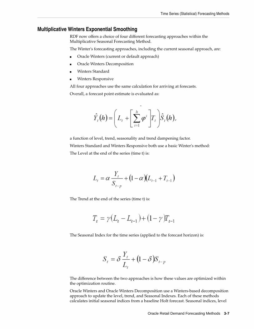
Time Series (Statistical) Forecasting Methods
Oracle Retail Demand Forecasting Methods 3-7
Multiplicative Winters Exponential SmoothingRDF now offers a choice of four different forecasting approaches within the Multiplicative Seasonal Forecasting Method.
The Winter's forecasting approaches, including the current seasonal approach, are:
■ Oracle Winters (current or default approach)
■ Oracle Winters Decomposition
■ Winters Standard
■ Winters Responsive
All four approaches use the same calculation for arriving at forecasts.
Overall, a forecast point estimate is evaluated as:
a function of level, trend, seasonality and trend dampening factor.
Winters Standard and Winters Responsive both use a basic Winter's method:
The Level at the end of the series (time t) is:
The Trend at the end of the series (time t) is:
The Seasonal Index for the time series (applied to the forecast horizon) is:
The difference between the two approaches is how these values are optimized within the optimization routine.
Oracle Winters and Oracle Winters Decomposition use a Winters-based decomposition approach to update the level, trend, and Seasonal Indexes. Each of these methods calculates initial seasonal indices from a baseline Holt forecast. Seasonal indices, level

Time Series (Statistical) Forecasting Methods
3-8 Oracle Retail Demand Forecasting User Guide for the RPAS Classic Client
and trend are then updated in separate stages, using Winter's model as a basis for the updates. The difference between the two approaches is which parameters are optimized and in which stages seasonal indices are updated.
Oracle WintersOracle Winters is the current seasonal forecasting approach, which uses a combination of Winters approach and decomposition. Decomposition allows level and trend to be optimized independently while maintaining a seasonal curve.
From sufficient data, RDF extracts seasonal indexes that are assumed to have multiplicative effects on the de-seasonalized series.
Oracle Winters DecompositionLike the Oracle Winters seasonal forecasting approach, Oracle Winters Decomposition uses a combination of Winters approach and decomposition.
From sufficient data, RDF extracts seasonal indexes that are assumed to have multiplicative effects on the de-seasonalized series.
The key difference between Oracle Winters and Oracle Decomposition is that the Seasonal smoothing parameter is also optimized, and the calculation of Seasonal Indices and de-seasonalizing of data is done with in the optimization routine for Oracle Winters Decomposition.
Also the optimization routine with in Oracle Winters Decomposition, while minimizing forecast errors, tends to weigh more recent Forecast errors heavier.
As with Oracle Winters, three parameters are used to control smoothing of level, trend, and seasonality.
Key differences between Oracle Winters and Oracle Winters Decomposition include:
■ Seasonal smoothing factor is optimized.
■ The optimization places more importance on recent sales than historical sales.
Note: The component describing the de-seasonalized values, which is multiplied by the seasonal index:
is the Holt model described above.
In this case, three parameters are used to control smoothing of the components of level, trend, and seasonality.
Note: The component describing the de-seasonalized values, which is multiplied by the seasonal index:
is the Holt model described above.
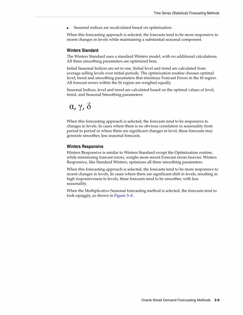
Time Series (Statistical) Forecasting Methods
Oracle Retail Demand Forecasting Methods 3-9
■ Seasonal indices are recalculated based on optimization.
When this forecasting approach is selected, the forecasts tend to be more responsive to recent changes in levels while maintaining a substantial seasonal component.
Winters StandardThe Winters Standard uses a standard Winters model, with no additional calculations. All three smoothing parameters are optimized here.
Initial Seasonal Indices are set to one. Initial level and trend are calculated from average selling levels over initial periods. The optimization routine chooses optimal level, trend and smoothing parameters that minimize Forecast Errors in the fit region. All forecast errors within the fit region are weighed equally.
Seasonal Indices, level and trend are calculated based on the optimal values of level, trend, and Seasonal Smoothing parameters:
When this forecasting approach is selected, the forecasts tend to be responsive to changes in levels. In cases where there is no obvious correlation in seasonality from period to period or where there are significant changes in level, these forecasts may generate smoother, less seasonal forecasts.
Winters ResponsiveWinters Responsive is similar to Winters Standard except the Optimization routine, while minimizing forecast errors, weighs more recent Forecast errors heavier. Winters Responsive, like Standard Winters, optimizes all three smoothing parameters.
When this forecasting approach is selected, the forecasts tend to be more responsive to recent changes in levels. In cases where there are significant shift in levels, resulting in high responsiveness to levels, these forecasts tend to be smoother, with less seasonality.
When the Multiplicative Seasonal forecasting method is selected, the forecasts tend to look squiggly, as shown in Figure 3–4.

Time Series (Statistical) Forecasting Methods
3-10 Oracle Retail Demand Forecasting User Guide for the RPAS Classic Client
Figure 3–4 Multiplicative Winters Exponential Smoothing
Additive Winters Exponential SmoothingRDF now offers a choice of four different Forecasting approaches within the Additive Seasonal Forecasting Method.
The Winters forecasting approaches, including the current seasonal approach, are:
■ Oracle Winters (current or default approach)
■ Oracle Winters Decomposition
■ Winters Standard
■ Winters Responsive
All four approaches use the same calculation for arriving at forecasts.
Overall, a forecast point estimate is evaluated as:
a function of level, trend, seasonality and trend dampening factor.
Winters Standard and Winters Responsive both use a basic Winter's method.
The Level at the end of the series (time t) is:
and the Trend at the end of the series (time t) is:

Time Series (Statistical) Forecasting Methods
Oracle Retail Demand Forecasting Methods 3-11
and the Seasonal Index for the time series (applied to the forecast horizon) is:
The difference between the two approaches is how these values are optimized within the optimization routine.
Oracle Winters and Oracle Winters Decomposition use a Winters-based decomposition approach to update the level, trend and Seasonal Indexes.
Refer to Multiplicative Winters Exponential Smoothing in this document for a description of each of the Forecasting Approaches.
Seasonal Exponential Smoothing (SeasonalES) In certain instances, it is known that seasonal models generally outperform non-seasonal models in forecast accuracy. When this is true (generally used for known seasonal items or for forecasts with a long horizon), it is advantageous to prevent AutoES from selecting from the Simple/Holt/Croston's methods. Choosing SeasonalES does just this. In instances where there exists too little data to create a seasonal forecast (less than 52 weeks of history), the SeasonalES method cascades to select between Simple/Holt/Croston. In all other instances, a seasonal model (Winter's or Seasonal Regression) is chosen. The following section has more information on Seasonal Regression.
Seasonal Regression A common benchmark in seasonal forecasting methods is sales last year. A sales last year forecast is based entirely on sales from the same time period of last year. Forecasting using only sales last year involves simple calculations and often outperforms other more sophisticated seasonal forecasting models. This method performs best when dealing with highly seasonal sales data with a relatively short sales history.
The seasonal models used in earlier releases of RDF (Additive and Multiplicative Winters) were designed to determine seasonality. However, they were not designed to work with sales histories of shorter than two years. Because sales histories of longer than two years are often difficult to obtain, many retail environments need a seasonal forecast that can accommodate sales data histories of between one and two years. In addition, the Additive and Multiplicative Winters models search for short-term trends and have difficulties with trends occurring inside the seasonal indices themselves. The current RDF Seasonal Regression forecasting model is designed to address these needs.
The Seasonal Regression Model uses simple linear regression with last year's data as the predictor variable and this year's sales as the target variable. The system determines the multiplicative and additive weights that best fit the data on hand. When optimizing the Seasonal Regression Model, the sales last year forecast is inherently considered, and it will automatically be used if it is the model that best fits

Time Series (Statistical) Forecasting Methods
3-12 Oracle Retail Demand Forecasting User Guide for the RPAS Classic Client
the data. If there have been significant shifts in the level of sales from one year to the next, the model learns that shift and appropriately weight last year's data (keeping the same shape from last year, but adjusting its scale).
As with other seasonal models, you can forecast demand for products with insufficient sales histories using this method if:
■ You paste in fake history as needed, providing a seasonal profile for the previous year.
■ You also forecast for a source level (with the same seasonality profile as the forecast item and with more than one year of history) using seasonal regression and spread these forecast results down to the member products.
The Seasonal Regression Model is included in the AutoES family of forecasting models, and is thus a candidate model that is selected if it best fits the data.
This method captures the trend of a series through the slope of the regression line while the series shifted by a cycle provides its seasonal profile. Using this method, the resulting forecast for the original series is calculated. The regression method provides a much better forecast of the series than was possible with the other exponential smoothing algorithms.
Based on the assumptions of the model that this method is trying to describe, versus the noisy data it is likely to receive, several exceptions to this regression technique are caught and corrected. First, since it is logically impossible to receive a negative value for the slope (such a value suggesting an inverse seasonality), whenever a negative slope is detected, the regression is rerun with the intercept fixed to zero. This guarantees that a positive slope is calculated and thus a more logical forecast is given.
The second noise-driven concession is to check the slope to determine if it is either too slight or too great. If this is the case, the method rejects itself out of hand and allows one of the other competing methods to provide the forecast.
Bayesian Information Criterion (BIC)Within AutoES, the model that minimizes the Bayesian Information Criterion (BIC) is selected as the final model. The BIC criterion attempts to balance model complexity with goodness-of-fit over the historical data period (between history start date and forecast start date). The BIC criterion rewards a model for goodness-of-fit and penalizes a model for its complexity. The complexity penalty is necessary to avoid over fitting.
There are various equivalent versions of the Bayesian Information Criterion, but RDF minimizes the following:
where n is the number of periods in the available data history, k is the number of parameters to be estimated in the model (a measure of model complexity), and s is the root mean squared error computed with one-step-ahead forecast errors resulting from the fitted model (a measure of goodness-of-fit). Note that since each member of the model candidate list is actually a family of models, an optimization routine to select optimal smoothing parameters is required to minimize s for each model form (that is, to select the best model).

Time Series (Statistical) Forecasting Methods
Oracle Retail Demand Forecasting Methods 3-13
Within RDF, a few modifications to the standard selection criteria have been made. These include reducing the number of parameters the Winter's model is penalized by discounting seasonal indices that have little impact on the forecast (multiplicative indices close to 1, additive indices close to 0). These changes tend to favor the seasonal models to a slightly higher degree that improves the forecasts on retail data, especially for longer forecast horizons.
AutoES FlowchartThe following procedure outlines the processing routine steps that the system runs through to evaluate each time series set to forecast using the AutoES method. See Figure 3–5, "AutoES Flowchart".
1. Filter all leading zeros in the input data that is within the training window.
2. Does the time series contain the minimum data points to qualify to forecast using the Croston's method? If yes, generate the forecast and statistics using the Croston's method, and move on to the next time series. If no, move on to Step 3.
3. Does the time series contain enough relevant data to generate a forecast? If yes, generate a forecast and statistics using the SimpleES method and move on to Step 4. If no, do not forecast, and go to the next time series.
4. Does the time series contain the minimum data points to qualify to forecast using the Holt method? If yes, generate a forecast and statistics using the Holt method and move on to Step 5. If no, move on to Step 9.
5. Does the time series contain more than 52 weeks of input data? If yes, generate a forecast and statistics using the Seasonal Regression method and move on to Step 6. If no, move on to Step 9.
6. Does the time series contain the minimum data points to qualify to forecast using Winters methods? If yes, move on to Step 7. If no, move on to Step 9.
7. Does the time series contain any data point with sales equal qualify to forecast using Additive Winters method? If yes, generate the forecast and statistics using the Additive Winters method, and move on to Step 9. If no, move on to Step 8.
8. Does the time series qualify to forecast using the Multiplicative Winters method? If yes, generate the forecast and statistics using both the Additive Winters and Multiplicative Winters methods, and move on to Step 9.
9. Compare all candidate forecasts using BIC Criterion.
10. Return the corresponding forecast and statistics for the system-selected forecast method, and move on to the next time series.

Time Series (Statistical) Forecasting Methods
3-14 Oracle Retail Demand Forecasting User Guide for the RPAS Classic Client
Figure 3–5 AutoES Flowchart
Automatic Forecast Level Selection (AutoSource)This section describes how the Automatic Forecast Level Selection (AutoSource) could help improve the accuracy of your forecasts.
In the system, one of the key elements to producing accurate forecasts is using the system's ability to aggregate and spread sales data and forecasts across the product and location hierarchies. Low selling or relatively new products can use aggregated data from similar products/locations at a higher level in the hierarchy, generate forecasts using this data, and then spread these higher level forecasts back down to provide more accurate forecasts. The difficulty comes in deciding which products/locations will benefit from this technique and from what level in the hierarchy these source level forecasts should be spread.
The Automatic Forecast Level Selection feature of the system automates the selection of best aggregation level (forecast source level) for each product/location combination. While providing invaluable information regarding the best aggregate level for source forecasts, the Automatic Forecast Level Selection process may be very CPU intensive. To solve this problem, the task of selecting best aggregation levels for product/location

Time Series (Statistical) Forecasting Methods
Oracle Retail Demand Forecasting Methods 3-15
combinations is decomposed and processed piecemeal during times when the computer would normally be idle. Identifying the best aggregation levels for sets of products and locations can be divided into a number of sub-problems:
■ Forecasting
■ Determining the best source level forecast
■ Status and scheduling
The Forecast Level Selection ProcessThe automatic source generation level selection subsystem selects the best source generation level for each product/location in a given final forecast level. In order to determine the best level, a final forecast is generated for each product/location using each candidate source generation level. As illustrated in Figure 3–6, a final forecast is generated by:
1. Aggregating up from the base level to the source level
2. Generating a source level forecast
3. Spreading the source-level forecast down to the final level
For example, assume base-level sales data is at the item/store level, the final forecast level is at the item/store level, and the candidate source generation level is at the style/store level. In this case, base-level sales data is aggregated from the item/store level up to the style/store level. A style/store forecast is generated, and the forecast data is spread back down to the item/store level. This forecast represents the final forecast.
Figure 3–6 Forecast Level Selection Process
Time Series (Statistical) Forecasting Methods
3-16 Oracle Retail Demand Forecasting User Guide for the RPAS Classic Client
Determining the Best Source Level ForecastThe selection of the best level is based on a train-test approach. In this process, historical data is used to generate a forecast for a test period for which actual sales data already exists. The forecast, generated over the train period, can be compared to the actual sales figures in the test period to calculate the Percent Absolute Error (PAE) between the two.
A final-level forecast is generated for each product/location combination using each potential source generation level. Each time a source level forecast is generated, a PAE is calculated for that level. If that PAE is better than the current best PAE (corresponding to the current best source generation level), the source generation level that generated that better PAE becomes the new best level.
Status and SchedulingIdentifying the best aggregation level for a given set of products and locations may take a significant amount of time (that is, an amount of time that is greater than the duration of the computer's shortest idle period). This task, however, can be partitioned meaning that the problem of selecting the best aggregation levels can be decomposed into smaller sub problems to be solved piecemeal during times when the computer would normally be idle.
For each product/location combination at the final forecast level, the problem consists of:
■ Generating forecasts at each unique aggregation level
■ Using the train-test approach to evaluate the percent absolute error statistics for each
One or more of these sub-tasks is performed during each period that the computer is idle. The best aggregation status keeps track of which sub problems have been performed and which sub problems remain. In this way, when the best aggregation procedure is run, the procedure knows what the next sub problem is.
Best aggregation level procedures are run during idle computer periods. The scheduling of the Automatic Forecast Level Selection process (AutoSource) must be integrated with the schedules of other machine processes. In general, you should select a schedule so that source generation level selection does not conflict with other activities. The following is an example of a typical schedule for the Automatic Forecast Level Selection process: Monday through Thursday, the selection process starts at midnight and runs for eight hours. On Friday and Saturday, the process is allowed to run for 20 hours. Sunday is reserved for generating forecasts.
Using the System-Selected Forecast LevelYou have the option of accepting the system-generated source level selection or manually selecting a different source level to be used. The value for the source forecast level can be manipulated in the Final Level worksheet of the Forecast Maintenance workbook. For each product/location combination, the best source forecast level identified by RDF appears in the Optimal Source Level measure on this worksheet. You can enable the use of this level by placing a check mark in the Pick Optimal Level measure for that product/location. The absence of a check mark in this measure causes the system to default to the Default Source Level or the Source Level Override value if this has been set by you.

Bayesian Forecasting
Oracle Retail Demand Forecasting Methods 3-17
Profile-Based ForecastingThe Profile-based forecasting method generates a forecast based on a seasonal profile. The profile may be loaded, manually entered, or generated by Curve. It can also be copied from another profile and adjusted.
Forecast MethodThe Profile-based forecasting method proceeds as follows:
1. The historical data and the profile are loaded.
2. The data are de-seasonalized using the profile and then fed to Simple method.
3. The alpha is capped by 0.5.
4. The Simple forecast is re-seasonalized using the profiles.
Profile-Based Method and New ItemsThe Profile-based forecasting method can be successfully used to forecast new items. In order to do that, we need to have a profile (which can be copied from an item that shares the same seasonality) and a number that specifies the de-seasonalized demand (DD value). The forecast is calculated using the DD value multiplied by the profile. The confidence interval is set to 1/3 of the DD value.
If the DD value is used to forecast, the history (if exists) of the product is ignored. Once we have enough history (number of data points exceed a global parameter), the forecast stops using the DD value and it defaults to the normal Profile Based method.
Bayesian ForecastingThe Bayesian Forecasting method is based on combining historic sales data with sales plan data. It is especially effective for new products with little or no historic sales data.
Your sales plan can incorporate expert knowledge in two ways — shape and scale.
■ Shape is the selling profile or lifecycle that can be derived from a sales plan. For example, the shape for certain fashion items might show sales ramping up quickly for the first four weeks and then trailing off to nothing over the next eight weeks.
■ Scale, or magnitude, of a sales plan is the total quantity expected to be sold over the plan's duration.
Bayesian Forecasting assumes that the shape that sales takes is known, but the scale is uncertain. In Bayesian Forecasting, when no sales history is available, the sales forecast figures are equal to the sales plan figures. At this point, there is no reason to mistrust the sales plan. As point of sale data becomes available, the forecast is adjusted and the scale becomes a weighted average between the initial plan's scale and the scale reflected by known sales history. Confidence in the sales plan is controlled by the amount of sales data on hand and a Bayesian sensitivity constant (Bayesian Alpha), which you can set between zero and infinity.
Unlike standard time series forecasting, which requires only sales history to produce a forecast, Bayesian Forecasting requires a sales plan and sales history (if available). Because of this difference, Bayesian Forecasting is not included in AutoES. You must select it manually as a forecasting method in Forecast Administration or Forecast Maintenance.
Obtaining accurate short life-cycle product forecasts is very difficult, and standard statistical time series forecasting models frequently do not offer an adequate solution
Bayesian Forecasting
3-18 Oracle Retail Demand Forecasting User Guide for the RPAS Classic Client
for many retailers. The following are major problems in automatically developing these forecasts:
■ The lack of substantial sales history for a product (which especially makes obtaining seasonal forecasts very difficult).
■ The difficulty of automatically matching a new product to a previous product or profile.
■ The inability to include planners' intuition into a forecasting model. For example, the overall sales level of the product, how quickly the product takes off, how the product's sales is affected by planned promotions.
Using a Bayesian approach, a short life-cycle forecasting algorithm was developed that begins with a product's seasonal sales plan (that is developed externally to the system by the planner). As sales information arrives during the first few days or weeks of the season, the model generates a forecast by merging the information contained in the sales plan with the information contained in the initial sales data. These forecast updates can be critical to a company's success and can be used to increase or cancel vendor orders.
As forecasting consultants and software providers, Oracle Retail assists clients in obtaining good forecasts for future demands for their products based upon historical sales data and available causal information. Depending on the information available, Oracle Retail's software supports various forms of exponential smoothing and regression based forecasting. Frequently, clients already have some expectations of future demands in the form of sales plans. Depending on the quality of their plans, they can provide very useful information to a forecasting algorithm (especially when only limited historical sales data is available). A forecasting algorithm was developed that merges a customer's sales plans with any available historical sales in a Bayesian fashion (that is, it uses new information to update or revise an existing set of probabilities.
Sales Plans versus Historic DataIn most retail situations, clients are interested in obtaining good product forecasts automatically with little or no human intervention. For stable products with years of historic sales data, our time series approaches (Simple, Holt, Winters, Regression based Causal, and so on) produce adequate results. The problem arises when attempting to forecast products with little or no history. In such instances, expert knowledge (generally in the form of sales plans) is required. Given that both sales plans and time series forecasts are available, an obvious question exists: When should the transition from sales plan to time series forecasting occur? In answering that question (in a particular scenario), suppose that we have determined that thirteen weeks of history is the transition point. Does that mean that at 12 weeks the time series results are irrelevant and that at 14 weeks the sales plan has no value? Our intuition tells us that instead of a hard-edge boundary existing; there is actually a steady continuum where the benefits from the sales plan decrease as we gather more historic sales data. This was the motivation for developing an approach that would combine the two forecasts in a reasonable manner.

Causal (Promotional) Forecasting Method
Oracle Retail Demand Forecasting Methods 3-19
Bayesian AlgorithmBayesian forecasting is primarily designed for product/location positions, for which a plan exists. These product/locations can be, but are not limited to: items new in the assortment, fashion items, and so on. The following guidelines should be followed:
1. No more than one plan should exist for a given product/location position. If multiple plans are to be set up for different time periods, the domain should be set up with different forecasting levels for each time period of interest.
2. Any time period with non-zero Actuals for a given product/location position should have a corresponding plan component. Otherwise, the system assumes a plan exists and equals zero and acts accordingly.
3. The time period of interest for the Bayesian algorithm starts with the first non-zero value of the plan or the history start date (whichever is more recent), and ends at the end of the forecast horizon.
LoadPlan Forecasting MethodLoadPlan Forecasting Method copies the measure that was specified as Data Plan in the Forecast Administration Workbook into the Forecast measure. This method does not generate confidence and cumulative intervals.
Copy Forecasting MethodCopy Forecasting Method copies the measure that was specified as Forecast Data Source in the Forecast Administration Workbook into the Forecast measure. This method does not generate confidence and cumulative intervals.
Causal (Promotional) Forecasting MethodCausal, or promotional, forecasting requires three input streams:
■ Time Series Data
■ Historical Promotional Calendar
■ Future Promotional Calendar
Promote decomposes the problem of promotional forecasting into two sub-tasks:
■ Estimating the effect that promotions have on demand
■ Forecasting baseline (that is no promotions) demand
To accomplish the first task, a stepwise regression sub-routine is used. This routine takes a time series and a collection of promotional variables and determine which variables are most relevant and what effect those relevant variables have on the series. Thus, the output from the algorithm is a selection of promotional variables and the effects of those variables on the series. In the second step, the time series is de-causalized using the promo effects. Then, AutoES is used to calculate the baseline demand. Once we know the effects and we have the baseline demand, we can generate a promotional forecast by applying the effects wherever the promotion is active in the future.
It should be noted that just because promotional forecasting is selected, it does not necessarily imply that a promotional forecast results. In some instances, no promotional variables is found to be statistically significant. In these cases, the forecast ends up equivalent to a standard time series forecasts. If you want to force in certain

Causal (Promotional) Forecasting Method
3-20 Oracle Retail Demand Forecasting User Guide for the RPAS Classic Client
promotional variables into the model, this can be managed through forecasting maintenance parameters.
The Oracle Retail experience in promotional forecasting has led us to believe that there are a few requirements that are necessary to successfully forecast retail promotions:
■ Baseline forecasts need to consider seasonality; otherwise normal seasonal demand is attributed to promotional effects.
■ Promotional Effects need to be able to be analyzed at higher levels in the retail product and location hierarchies. This produces cleaner signals and alleviates issues involved in forecasting new items and new stores and issues involving data sparsity.
■ Users need to be aware that the forecasting models cannot tell the difference between causal effects and correlated effects. What this means is that users should be wary of promotional effects attributed to an event that occurs at the same time every year. The system cannot distinguish between the promotional effect and the normal seasonality of the product. The same can be said for any two events that always occur at the same time. The combined effect is most likely attributed to one or the other event.
The Causal Forecasting AlgorithmFor purposes of understanding the algorithm, a promotional variable is defined as a causal event that is only active for certain series at certain points in time. It is assumed that these events are entered into the system independently of the forecasting algorithm and that a vehicle exists for determining which promotional variable are relevant to a particular series.
The core of the causal forecasting algorithm uses a stepwise regression sub-routine. This routine takes a time series and a collection of promotional variables, and it determines which variables are most relevant and what effect those relevant variables have on the series. Thus, the output from the algorithm is a selection of promotional variables and the effects of those variables on the series.
Causal variable types define how causal variables are treated in the causal model fitting process (which includes a call to the lower level regression engine) and the forecast generation process where the model is used to extend the forecast over the forecast horizon. See the Promote (Promotional Forecasting) chapter for information on each of the causal variable types:
■ Automatic
■ Force In The Model
■ Disabled
■ Override All
■ Override Future
■ Override Higher Level

Causal (Promotional) Forecasting Method
Oracle Retail Demand Forecasting Methods 3-21
Causal Forecasting ProcessThe causal forecasting algorithm itself lies in the AutoES binary code, and it executes in the following manner.
1. The binary reads the history of the time series.
2. The binary reads the type of each promotional variable into the system.
3. The binary reads in all the promotional variables that apply to the series.
4. The binary creates an internal promotional variable to allow the modeling of trend.
5. Promotional variables, internal promotional variables, promotional variable types, and the series itself are passed to the stepwise regression routine with the historic data serving as the dependent variables.
6. If the regression finds no significant promotional variables, the casual method is considered to have failed to fit. In this case, the standard time series methods are used to generate a forecast and skips to step 14.
7. The fit at time t, fit(t), is defined in terms of bo, the intercecpt of the regression, b1, the effect corresponding to promotional variable i, and pi(t), is the value of promo variable I, in time t as:
fit(t) = bo + å bo*pi(t)
8. The Time Series is de-causalized in the fit region of the history by removing the causal effects. That is, subtracting the additive causal effects for the product/location/time positions where the corresponding promo variables are on.
9. A seasonal model is fitted to the de-causalized series. The seasonal model is the winner of a competition between SeasonalES, Additive Winters, and Multiplicative Winters. The RMSE is determined across the fit region on the de-causalized series and the winning model is the one that produces the least RMSE.
10. The winning seasonal model is then used to determine the seasonal forecast by applying the fit(t) function across the forecast horizon. This forecast is also exported as the baseline forecast (that is forecast without any causal influences).
11. The forecast is obtained by re-causalizing the seasonal forecast. This is done by adding back the additive causal effects for the product/location/time positions where the corresponding promo variables are on in the forecast region.
12. The binary writes the winning promotional variables effects back to the database.
13. The selected model is recorded in the database.
14. The binary records the forecast and the baseline in the database.

Causal (Promotional) Forecasting Method
3-22 Oracle Retail Demand Forecasting User Guide for the RPAS Classic Client
FlowchartFigure 3–7 summarizes the Causal Forecasting process.
Figure 3–7 Causal Forecasting Process

Causal Forecasting with External Baseline
Oracle Retail Demand Forecasting Methods 3-23
Causal Forecasting with External BaselineRather than use a sales history that may not have sufficient or accurate data, users can load an external baseline into the RDF Causal Engine instead. External baselines are often generated using data that is rolled up to a higher dimension than SKU/store, providing a greater depth of data and hence a less-noisy sales history. The sales data used to generate the external baseline can be corrected for out-of-stock, promotional, and other short-term event information using Preprocessing. These external baselines are then spread back to the SKU/store level and then loaded in the RDF Causal Engine. The Engine then uses this external baseline (rather than the causal baseline) along with the historic promotional data and future planned promotions data to create the system forecast, which is the external baseline with the lifts, which were calculated from the promotional data, applied on top.
Causal Forecasting Using External Baseline ProcessWhen an external baseline is used, the AutoES binary code executes in the following manner:
1. The binary reads the history of the time series.
2. The binary reads the type of each promotional variable into the system.
3. The binary reads in all the promotional variables that apply to the series.
4. The binary creates an internal promotional variable to allow the modeling of trend.
5. Promotional variables, internal promotional variables, promotional variable types, and the series itself are passed to the stepwise regression routine with the historic data serving as the dependent variables.
6. If the regression finds no significant promotional variables, the casual method is considered to have failed to fit. In this case, the forecast equals the external baseline.
7. The fit at time t, fit(t), is defined in terms of bo, the intercecpt of the regression, b1, the effect corresponding to promotional variable i, and pi(t), is the value of promo variable I, in time t as:
fit(t) = bo + å bo*pi(t)
8. The forecast is obtained by re-causalizing the external baseline. This is done by adding back the additive causal effects for the product/location/time positions where the corresponding promo variables are on in the forecast region.
9. The binary writes the winning promotional variables effects back to the database.
10. The selected model is recorded in the database.
11. The binary records the forecast and the baseline in the database.
Causal Forecasting for Short Lifecycle ItemsTo forecast short lifecycle, promotional items, Causal deprices, depromotes, and smoothes the forecasting data source to generate the short lifecycle forecast causal baseline.
In essence, causal forecasting uses the external baseline, where the generation of the baseline and the promotional lifts is modified for items with short lifecycle.
First, the external baseline is generated. Then the forecast data source is depriced, depromoted and smoothed. The resulting feed is aggregated and then spread down

Causal Forecasting with External Baseline
3-24 Oracle Retail Demand Forecasting User Guide for the RPAS Classic Client
using rate of sales as a profile to create a lifecycle curve. The lifecycle curve is shifted and stretched or shrunk to fit the new season length. This curve represents the pre-season baseline forecast. In season, the pre-season forecast serves as a forecast plan to the Bayesian forecasting method. The Bayesian forecast is the causal external baseline for short lifecycle items.The next step is to calculate the promotional lifts. To do this, the promotional lifts are filtered from the historical sales, and applied on top of the item's rate of sale. The resulting measure is regressed against the promotional variables to determine the promotion effects. Finally, the promotion effects are applied on top of the short lifecycle causal baseline to generate the final forecast.
Causal Forecasting at the Daily LevelThe causal forecasting at the daily level is calculated by spreading the weekly causal forecast down to day. The spreading utilizes causal daily profiles, thus obtaining a causal forecast at the day granularity.
The daily casual forecast process executes in the following manner:
1. Preprocess the day level promotional variables by multiplication with daily profiles. Aggregate the preprocessed continuous day level promotional variables to the week level.
2. Calculate the causal forecast at the weekly level. Set promotional effects if desired. Use the RDF causal engine to generate the forecast.
3. Calculate the multiplicative promotional effects at the item/store level for every promo variable. The effects can be either:
■ Manually preset (See Step 1).
■ Calculated. When calculating the causal forecast, the calculated causal effects are written back to the database. If the effects are calculated at higher level than item/store, the effects are replicated down to item/store since the effects are multiplicative. If source level forecasting is used and causal method is used both at the source level and at the final level, the effects from the final level is used.
4. Daily profiles are calculated using the Curve module. Since as much history as possible is used and is averaged over seven days, it's assume that these profiles are de-causalized. The de-causalized daily profiles capture the day of week effect and should be quite stable.
5. Causal effects are applied to the daily profiles. The profiles are multiplied by the causal effects and then the profiles have to renormalize.
ExampleFor every item/store combination, calculate a normal week-to-day profile based on historic data. Note that this profile is already computed for spreading the weekly forecasts to the day level. Suppose for a certain product, the profile is as follows:
Mon Tues Wed Thu Fri Sat Sun Week
10% 10% 10% 10% 20% 30% 10% 100%

Causal Forecasting with External Baseline
Oracle Retail Demand Forecasting Methods 3-25
Suppose that in the past, the promotion was held on Wednesday, Thursday, and Friday of week w6:
Then the continuous weekly indicator for this promotion in w6 should be set to 0.4, which is the sum of the weights of Wednesday, Thursday, and Friday.
Now assume that the same promotion is held in a future week (w36), but only on Thursday:
Then the continuous weekly indicator for w36 should be set to 0.1, which is the weight of Thursday only.
The approach to use the continuous promotion indicators to generate an accurate causal forecast at the day level is as follows:
■ Calculate the weekly multiplicative effect for the promotion using the standard causal forecasting system with continuous indicators.
■ Calculate the forecast for w36 using the standard causal forecasting system with continuous indicators.
■ Update the week-to-day profile of w36 so that the weight of Thursday is doubled (the multiplicative factor is 2):
■ Normalize the profile for w36:
Finally, spread the forecast of w36 using the normalized profile.
Final Considerations About Causal ForecastingIn the Oracle Retail approach to causal forecasting, the causal effects are obtained by fitting a stepwise linear regression model that determines which variables are most relevant and what effect those relevant variables have on the series. The data used to fit the regression is the fit history of each time series, so basically a model is fit per time series. A problem arises due to potential lack of significant data (that is, when a promotional variable is not represented in the history, but it is present in the forecast region). In that case, the effect for that variable would not be computed at all, thus affecting the accuracy of the forecast. There are a few solutions that make use of the effects from other similar time series. One solution would be to do source level causal forecasting and then spread down to the final level. This would be equivalent to using the effects at the source level for time series that have no causal variable instances in
Mon Tues Wed Thu Fri Sat Sun
P P P
Mon Tues Wed Thu Fri Sat Sun
P
Mon Tues Wed Thu Fri Sat Sun Week
10% 10% 10% 20% 20% 30% 10% 110%
Mon Tues Wed Thu Fri Sat Sun Week
9% 9% 9% 18% 18% 27% 9% 100%

Causal Forecasting with External Baseline
3-26 Oracle Retail Demand Forecasting User Guide for the RPAS Classic Client
the history. This has a serious conceptual drawback-by aggregating the promotional variables at the source level, we would force the effects on the other time series in the same aggregation class that would otherwise not have the causal variables on at the same time. An alternate solution is whenever a causal effect cannot be computed because of lack of significant data; an averaged effect from another time-series in the same aggregation class is going to be used instead. See Table 7–1, " Causal Variable Types" on page 7-8 for information on the Override Higher Level type.
4
Setting Forecast Parameters 4-1
4Setting Forecast Parameters
The Forecast workbook template group allows you to perform functions related to statistical time series forecasting. This chapter provides information on defining and maintaining the parameters that govern the generation of forecasts in RDF.
Refer to Appendix A, "Appendix: RDF Workbooks"for a complete list of RDF workbooks, and their respective tabs, worksheets, and measures.
Forecast Administration WorkbookThis section describes the components of the Forecast Administration workbook.
Basic versus Advanced TabsForecast Administration is the first workbook used in setting up RDF to generate forecasts. It provides access to forecast settings and parameters that govern the whole domain (database). These settings and parameters are divided into two areas, accessed through the Basic and Advanced tabs beneath main toolbar.
The Basic tab is used to establish a final level forecast horizon, the commencement and frequency of forecast generation, and the specification of aggregation levels (Source Levels) and spreading (Profile) methods used to yield the final level forecast results.
The Advanced tab is used to set default values for parameters affecting the algorithm and other forecasting techniques used to yield final level and source level forecasts, thus eliminating the need to define these parameters individually for each product and location. If certain products or locations require parameter values other than the defaults, these fields can be amended on a case-by-case basis in the Forecast Maintenance Workbook.
Final versus Source Level ForecastsOften, forecast information is required for items at a very low level in the hierarchy. However, problems can arise in that data is often too sparse and noisy to identify clear patterns at these lower levels. For this reason, it sometimes becomes necessary to aggregate sales data from a low level to a higher level in the hierarchy in order to generate a reasonable forecast. Once this forecast is created at the higher or source level, the results can be allocated to the lower or final level dimension based on the lower level's relationship to the total.
In order to spread this forecast information back down to the lower level, it is necessary to have some idea about the relationship between the final level and the source level dimensions. Often, an additional interim forecast is run at the low level in order to determine this relationship. Forecast data at this low level might be sufficient

Forecast Administration Workbook
4-2 Oracle Retail Demand Forecasting User Guide for the RPAS Classic Client
to generate reliable percentage-to-whole information, but the actual forecast numbers are more robust when generated at the aggregate level.
The Final Level worksheet represents forecast parameters for the lower (final) level, the level to which source forecast values are ultimately spread. Forecast data must appear at some final level in order for the data to be approved or exported to other systems. The Source Level worksheet represents the default values for forecast parameters at the more robust aggregate (source) level.
Forecasting Methods Available in Oracle Retail Demand ForecastingA forecasting system's main goal is to produce accurate predictions of future demand. The RDF solution utilizes the most advanced forecasting algorithms to address many different data requirements across all retail verticals. Furthermore, the system can be configured to automatically select the best algorithm and forecasting level to yield the most accurate results.
The following section summarizes the use of the various forecasting methods employed in the system. This section is referenced throughout this document when the selection of a forecasting method is required in a workflow process. Some of these methods may not be visible in your solution based on configuration options set in the RPAS Configuration Tools. More detailed information on these forecasting algorithms is provided in Chapter 3, "Oracle Retail Demand Forecasting Methods."
Average RDF uses a simple average model to generate forecasts.
Moving Average RDF uses a simple moving average model to generate forecasts. You can specify a Moving Average Window length.
AutoESRDF fits the sales data to a variety of exponential smoothing models of forecasting, and the best model is chosen for the final forecast.
The candidate methods considered by AutoES are:
The final selection between the models is made according to a performance criterion (Bayesian Information Criterion) that involves a trade-off between the model's fit over the historic data and its complexity.
SimpleESRDF uses a simple exponential smoothing model to generate forecasts. SimpleES ignores seasonality and trend features in the demand data and is the simplest model of the exponential smoothing family. This method can be used when less than one year of historic demand data is available.
SimpleES Seasonal Regression
IntermittentES Causal
TrendES No Forecast
Multiplicative Seasonal Bayesian
Additive Seasonal Profile-based
SeasonalES Components

Forecast Administration Workbook
Setting Forecast Parameters 4-3
IntermittentESRDF fits the data to the Croston's model of exponential smoothing. This method should be used when the input series contains a large number of zero data points (that is, intermittent demand data). The original time series is split into a Magnitude and Frequency series, and then the SimpleES model is applied to determine level of both series. The ratio of the magnitude estimate over the frequency estimate is the forecast level reported for the original series.
Simple/IntermittentESSimple/IntermittentES is a combination of the SimpleES and IntermittentES methods. This method applies the SimpleES model unless a large number of zero data points are present, in which case the Croston's model is applied.
TrendESRDF fits the data to the Holt model of exponential smoothing. The Holt model is useful when data exhibits a definite trend. This method separates base demand from trend, and then provides forecast point estimates by combining an estimated trend and the smoothed level at the end of the series. For instance, where the forecast engine cannot produce a forecast using the TrendES method, the Simple/IntermittentES method is used to evaluate the time series.
Multiplicative SeasonalAlso referred to as Multiplicative Winters Model, this model extracts seasonal indices that are assumed to have multiplicative effects on the un-seasonalized series.
Additive SeasonalAlso referred to as Additive Winters Model, this model is similar to the Multiplicative Winters model, but is used when zeros are present in the data. This model adjusts the un-seasonalized values by adding the seasonal index (for the forecast horizon).
SeasonalESThis method, a combination of several Seasonal methods, is generally used for known seasonal items or forecasting for long horizons. This method applies the Multiplicative Seasonal model unless too many zeros are present in the data, in which case the Additive Winters model of exponential smoothing is used. If less than two years of data is available, a Seasonal Regression model is used. If there is too little data to create a seasonal forecast (in general, less than 52 weeks), the system selects from the SimpleES, TrendES, and IntermittentES methods.
Seasonal Regression Seasonal Regression cannot be selected as a forecasting method, but is a candidate model that is used only when the SeasonalES method is selected. This model requires a minimum of 52 weeks of history to determine seasonality. Simple Linear Regression is used to estimate the future values of the series based on a past series. The independent variable is the series history one-year or one cycle length prior to the desired forecast period, and the dependent variable is the forecast. This model assumes that the future is a linear combination of itself one period before plus a scalar constant.
Causal Causal is used for promotional forecasting and can only be selected if Promote is implemented. Causal uses a Stepwise Regression sub-routine to determine the promotional variables that are relevant to the time series and their lift effect on the

Forecast Administration Workbook
4-4 Oracle Retail Demand Forecasting User Guide for the RPAS Classic Client
series. AutoES utilizes the time series data and the future promotional calendar to generate future baseline forecasts. By combining the future baseline forecast and each promotion's effect on sales (lift), a final promotional forecast is computed. For instances where the forecasting engine cannot produce a forecast using the Causal method, the system evaluates the time series using the SeasonalES method.
To forecast short lifecycle, promotional items, Causal deprices, depromotes, and smoothes the forecasting data source to generate the short lifecycle forecast causal baseline. The promotion effects are calculated using the same Stepwise Regression code as Causal. However, the promo lifts are first filtered from the sales, and applied on top of the item's rate of sale. The resulting measure is regressed against the promotional variables to determine the promotion effects. Finally, the promotion effects are applied on top of the short lifecycle baseline to generate the final forecast.
No ForecastNo forecast is generated for the product/location combination.
BayesianUseful for short lifecycle forecasting and for new products with little or no historic sales data, the Bayesian method requires a product's known sales plan (created externally to RDF) and considers a plan's shape (the selling profile or lifecycle) and scale (magnitude of sales based on Actuals). The initial forecast is equal to the sales plan, but as sales information comes in, the model generates a forecast by merging the sales plan with the sales data. The forecast is adjusted so that the sales magnitude is a weighted average between the original plan's scale and the scale reflected by known history. A Data Plan must be specified when using the Bayesian method. For instances where the Data Plan equals zero (0), the system evaluates the time series using the SeasonalES method.
Profile-basedRDF generates a forecast based on a seasonal profile that can be created in RPAS or legacy system. Profiles can also be copied from another profile and adjusted. Using historic data and the profile, the data is de-seasonalized and then fed to the SimpleES method. The Simple forecast is then re-seasonalized using the profiles. A Seasonal Profile must be specified when using the Profile-Based method. For instances where the Seasonal Profile equals zero, the system evaluates the time series using the SeasonalES method.
ComponentsThe Components forecast method multiplies pre-calculated baseline, promotional lifts, and regular price lifts to generate the forecast. These components are specified in Forecast Administration workbook, Advanced Settings tab, Final Level Parameters worksheet. The following table lists the components and their referenced measures.
Intervals are not generated and need to be provided. This method is useful when the forecast components are available since the forecast can be quickly generated.
Component Measure
Baseline Components - Baseline
Regular Price Lifts Components - Regular Price Lifts
Promotional Lifts Components - Promotional Lifts
Interval Components - Baseline Interval

Forecast Administration Workbook
Setting Forecast Parameters 4-5
Creating a Forecast Administration Workbook Use the following procedure, to create a Forecast Administration Workbook.
1. Within the Master or Local Domain, select New from the File menu.
2. Select the Forecast tab to display a list of workbook templates for statistical forecasting.
3. Select Forecast Administration.
4. Click OK.
5. The Forecast Administration wizard opens and prompts you to select the level of the final forecast. The final forecast level is a level at which approvals and data exports can be performed. Depending on your organization's setup, you may be offered a choice of several final forecast levels. Make the appropriate selection.
6. Click Finish to open the workbook.
Window Descriptions for the Forecast Administration WorkbookThe following sections describe the components of the Forecast Administration workbook.
Basic Settings Workflow TabThe Basic Settings workflow tab contains forecast administration settings. On the Basic Settings workflow tab, there are two worksheets:
■ Final Level Worksheet - Basic Settings
■ Final and Source Level Parameters Worksheet - Basic Settings
Final Level Worksheet - Basic SettingsThe Final Level worksheet allows you to set the forecast horizon information, frequency of review, and all default parameters for the lower or final level forecast (the level to which aggregate forecast data is ultimately spread). Forecast approvals and data exports can only be performed on forecasts at a final level. Figure 4–1 provides an example of a view of the Final Level Parameters worksheet in a master domain with three partitions/local domains, partitioned based on group.
Figure 4–1 Final Level Parameters Worksheet

Forecast Administration Workbook
4-6 Oracle Retail Demand Forecasting User Guide for the RPAS Classic Client
Measures: Final Level Worksheet - Basic SettingsThe Final Level Worksheet - Basic Settings contains the following measures:
Default Approval MethodThis field is a list from which you select the default automatic approval policy for forecast items. Valid values are:
Default Source LevelThe pick list of values displayed in this field allows you to change the forecast level that is used as the primary level to generate the source forecast. The source levels are set up in the RPAS Configuration Tools. A value from the pick list is required in this field at the time of forecast generation.
Forecast CycleThe Forecast Cycle is the amount of time (measured in days) that the system waits between each forecast generation. Once a scheduled forecast has been generated, this field is used to automatically update the Next Run Date field. A non-zero value is required in this field at the time of forecast generation.
Forecast Start DateThis is the starting date of the forecast. If no value is specified at the time of forecast generation, the system uses the data/time at which the batch is executed as the default value. If a value is specified in this field and it is used to successfully generate the batch forecast, this value is cleared.
Forecast LengthThe Forecast Length is used with the Forecast Start Date to determine forecast horizon. The forecast length is based on the calendar dimension of the final level. For example, if the forecast length is to be 10 weeks, the setting for a final level at day is 70 (10 x 7 days).
Next Run DateThe Next Run Date is the date on which the next batch forecast generation process automatically runs. RDF automatically triggers a set of batch processes to be run at a pre-determined time period. When a scheduled batch is run successfully, the Next Run Date automatically updates based on the Start Date value and the Forecast Cycle. No value is required in this field when the Run Batch Forecast Workbook wizard is used to generate the forecast or if the batch forecast is run from the back-end of the domains using the override True option. See the Oracle Retail Demand Forecasting Implementation Guide for more information on forecast generation.
Field Description
Manual The system-generated forecast is not automatically approved. Forecast values must be manually approved by accessing and amending the Forecast Approval Workbook.
Automatic The system-generated quantity is automatically approved as-is.
By Alert This list of values may also include any Forecast Approval alerts that have been configured for use in the forecast approval process. Alerts are configured during the implementation. See the Oracle Retail Predictive Application Server Configuration Tools User Guide for more information on the Alert Manager.

Forecast Administration Workbook
Setting Forecast Parameters 4-7
Forecast Data SourceThis is a read-only value that displays the sales measure (the measure name) that is the data used for the generation of forecasts (for example, POS). The measure that is displayed here is determined at configuration time in the RPAS Configuration Tools. Different Data Sources can be specified for the Final and Source Levels.
Final and Source Level Parameters Worksheet - Basic SettingsThe Final and Source Level worksheet allows you to set the default parameters that are common to both the final and source level forecasts.
Figure 4–2 Final and Source Level Parameters Worksheet
Measures: Final and Source Level Parameters Worksheet - Basic SettingsThe Final and Source Level Parameters Worksheet - Basic Settings contains the following measures:
Forecast Data SourceThis is a read-only value that displays the sales measure (the measure name) that is the data used for the generation of forecasts (for example, POS). The measure that is displayed here is determined at configuration time in the RPAS Configuration Tools. Different Data Sources can be specified for the Final and Source Levels.
Default History Start DateThis field indicates to the system the point in the historical sales data at which to use in the forecast generation process. If no date is indicated, the system defaults to the first date in your calendar. It is also important to note that the system ignores leading zeros that begin at the history start date. For example, if your history start date is January 1, 1999 and an item/location does not have sales history until February 1, 1999, the system considers the starting point in that item/location's history to be the first data point where there is a non-zero sales value. Different History Start Dates can be specified for the Final and Source Levels.
Data PlanUsed in conjunction with the Bayesian forecast method, Data Plan is used to input the measure name of a sales plan that should be associated with the final level forecast. Sales plans, when available, provide details of the anticipated shape and scale of an item's selling pattern. If the Data Plan is required, this field should include the measure name associated with the Data Plan.

Forecast Administration Workbook
4-8 Oracle Retail Demand Forecasting User Guide for the RPAS Classic Client
Default Forecast MethodThe Default Forecast Method is a complete list of available forecast methods from which you can select the primary forecast method that is used to generate the forecast. A summary of methods is provided in Forecasting Methods Available in Oracle Retail Demand Forecasting. The chapter, Oracle Retail Demand Forecasting Methods, covers each method in greater detail. It is important to note that Causal should not be selected unless the forecast level was set as a Causal level during the configuration. See the Oracle Retail Demand Forecasting Configuration Guide for more information on configurations using the Causal forecast method.
Seasonal ProfileUsed in conjunction with the Profile-Based forecasting method, this is the measure name of the seasonal profile that is used to generate the forecast at either the source or final level. Seasonal profiles, when available, provide details of the anticipated seasonality (shape) of an item's selling pattern. The seasonal profile can be generated or loaded, depending on your configuration. The original value of this measure is set during the configuration of the RDF solution.
Spreading ProfileUsed for Source Level Forecasting, the value of this measure indicates the profile level that is used to determine how the source level forecast is spread down to the final level. No value is needed to be entered at the final level. For dynamically generated profiles, this value is the number associated with the final profile level (for example, 01)—note that profiles 1 through 9 have a zero (0) preceding them in Curve—this is different than the forecasting level numbers.
For profiles that must be approved, this is the measure associated with the final profile level. This measure is defined as apvp +level (for example, apvp01 for the approved profile for level 01 in Curve).
Source Level Forecast Data Source You can specify a measure to serve as a forecast data source at the source levels. If the measure is left blank for a certain source level the source measure from the corresponding final level is used.
Source Level History Start DateThis is the starting date for historical sales data at the source level. For example, if your system start date is January 1, 2003, but you only want to use historical sales data from the beginning of 1999, you need to set your History Start Date to January 1, 1999. Only history after this date is used for generating the forecast. The default is the system start date unless otherwise specified. If sales data is collected weekly or monthly, RDF generates forecasts only using data from sales periods after the one containing the history start date.
It is also important to note that the system ignores leading zeros that begin at the history start date. For example, if your history start date is January 1, 1999, and an item/location does not have sales history until February 1, 1999, the system considers the starting point in that item/location's history to be the first data point where there is a non-zero sales value.
Note: History start dates for final and source levels can be different.

Forecast Administration Workbook
Setting Forecast Parameters 4-9
Advanced Settings Workflow TabThe Forecast Administration Advanced Settings workflow tab is used to set parameters related to either the data that is stored in the system or the forecasting methods that are used at the final or source levels. The parameters on this workflow tab are not as likely to be changed on a regular basis as the ones on the Basic Settings workflow tab.
Final Level Parameters Worksheet - Advanced SettingsThe Final Level worksheet allows you to set the advanced parameters for the final level forecasts. Figure 4–3 provides an example of a view of this worksheet in a master domain with three partitions/Local Domains, partitioned based on group.
Figure 4–3 Final Level Parameters Worksheet
Measures: Final Level Parameters Worksheet - Advanced SettingsThe Final Level Parameters worksheet - Advanced Settings contains the following measures:
Components - BaselineThis measure stores the name of the measure that serves as baseline in the Components forecasting measure. If no measure is specified, the Components forecasting method assesses the value as one (1).
Components - Baseline IntervalThis measure stores the name of the measure that serves as baseline interval in the Components forecasting measure. If no measure is specified, the Components forecasting method assesses the value as one (1).

Forecast Administration Workbook
4-10 Oracle Retail Demand Forecasting User Guide for the RPAS Classic Client
Components - Regular Price LiftsThis measure stores the name of the measure that serves as regular price lifts in the Components forecasting measure. If no measure is specified, the Components forecasting method assesses the value as one (1).
Components - Promotional LiftsThis measure stores the name of the measure that serves as promotional lifts in the Components forecasting measure. If no measure is specified, the Components forecasting method assesses the value as one (1).
Days to Keep ForecastsThis field is used to set the number of days that the system stores forecasts based on the date/time the forecast is generated. The date/time of forecast generation is also referred to as birth date of the forecast. A forecast is deleted from the system if the birth date plus the number of days since the birth date is greater than the value set in the Days to Keep Forecast parameter. This process occurs when either the Run Batch Forecast Workbook wizard is used to generate the forecast or when PreGenerateForecast is executed.
When you start the Run Batch Forecast Workbook, one of the first steps that RDF takes is to remove forecasts older than the value given in the Days to Keep Forecasts parameter. RDF uses the value of that parameter in your local domain. However, because forecasts are registered globally, the Forecast Delete has a global effect. That is, if you set the parameter to some low value, for example one day, all forecasts in all local domains older than one day are removed. This can adversely impact other users of the system if done without consideration.
When the PreGenerate utility is used, typically for automated batch production of forecasts, RDF uses the value for the Days to Keep Forecasts parameter in the first local domain. Again, if this is set to a value that is not expected by the other users, it can cause unintended disruption.
See the Oracle Retail Demand Forecasting Implementation Guide for more information on PreGenerateForecast.
Default Keep Last ChangesThis field is a list from which you select the default change policy for forecast items. Valid values are:
Field Description
Keep Last Changes (None)
There are no changes that are introduced into the adjusted forecast.
Keep Last Changes (Total)
Considers only the Last Approved Forecast in determining change policy. For each forecast item/week-combination, RDF automatically introduces the same quantity that was approved in the Last Approved Forecast into the change only if that quantity differed from that in the Last System Forecast. If the quantities are the same, RDF introduces the current system-generated forecast into the adjusted forecast.
Keep Last Changes (Diff)
Considers both the Last System Forecast and the Last Approved Forecast in determining approval policy. For each forecast item/week-combination, RDF determines the difference between the Last System Forecast and the Last Approved Forecast. This difference (positive or negative) is then added to the current system forecast and calculated as the adjusted forecast.

Forecast Administration Workbook
Setting Forecast Parameters 4-11
Generate Baseline ForecastsA check should be indicated in this field (set to True) if the baseline forecast is to be generated to be viewed in any workbook. This parameter should be set if the level is used for Causal forecasting and the baseline is needed for analysis purposes.
Generate Cumulative IntervalA check in this field (set to True) specifies whether you want RDF to generate cumulative intervals (this is similar to cumulative standard deviations) during the forecast generation process. Cumulative Intervals are a running total of Intervals and are typically required when RDF is integrated with the Oracle Retail Merchandising System. If you do not need cumulative intervals, you can eliminate excess processing time and save disk space by clearing the check box. The calculated cumulative intervals can be viewed within the Forecast Approval Workbook.
Generate IntervalsA check in this field (set to True) indicates that intervals (similar to Standard Deviations) should be stored as part of the batch forecast process. Intervals can be displayed in the Forecast Approval Workbook. If you do not need intervals, excess processing time and disk space may be eliminated by clearing the check box. For many forecasting methods, intervals are calculated as standard deviation but for Simple, Holt, and Winters the calculation is more complex. Intervals are not exported.
Generate MethodsA check in this field (set to True) indicates that when an ES forecast method is used, the chosen forecast method for each fitted time series should be stored. The chosen method can be displayed in the Forecast Approval Workbook.
Generate ParametersA check in this field (set to True) indicates that the alpha, level, and trend parameters for each fitted time series should be stored. These parameters can be displayed in the Forecast Approval Workbook.
Interval Cap Lower RatioThe value entered in this field multiplied by the forecast represents the lower bound of the confidence interval for a given period in the forecast horizon.
Interval Cap Upper RatioThe value entered in this filed multiplied by the forecast represents the upper bound of the confidence interval for a given period in the forecast horizon.
Item End Date ActionThis parameter allows the option for items with end dates within the horizon to have zero demand applied to time series before or after the interim forecast is calculated. The two options are:
Keep Last Changes (Ratio)
Considers both the Last System Forecast and the Last Approved Forecast in determining change. For each forecast item/week-combination, RDF determines the difference between the Last System Forecast and the Last Approved Forecast. This difference is expressed as a percentage. This same percentage is used to calculate the adjusted forecast.
Field Description

Forecast Administration Workbook
4-12 Oracle Retail Demand Forecasting User Guide for the RPAS Classic Client
Like TS Duration (Periods)The Like TS Duration is the number of periods of history required, after which RDF stops using the substitution method and starts using the system forecast generated by the forecast engine. A value must be entered in this field if using Like-item/Sister-Store functionality. When the difference between the forecast start date and the history start date is greater than the Like TS Duration, RDF starts using the system forecast for the item.
The Like TS Duration determines for how long RDF applies the Like-item/Sister-Store functionality. In general, the difference between history start date and the forecast start date is compared to the Like TS Duration. If the difference is larger than the Like TS Duration, it means that the new item has been selling for a period long enough, such that RDF can create the forecast based on its own history.
The forecast start date has an override, which is usually used whenever the forecast start date is checked.
However, in the case of Like-item/Sister-Store, if the override references a date prior to the forecast start date, the forecast start date - instead of the override - is used when calculating the difference and comparing it to the Like TS Duration.
The reason behind this exception is that the override does not change unless it is initiated by a user. Hence the difference between forecast start date override and history start date is always the same, so the Like-item functionality is always in effect.
If the override is ignored, the forecast start date is advancing every period, so the difference between it and history start date is always growing. Eventually it will become larger than the Like TS Duration, and thus turning off the Like-item functionality for the item.
Store Interim ForecastA check should be placed in this field (set to True) if the interim forecast is stored. The Interim Forecast is the forecast generated at the Final Level. This forecast is used as the Source Data within Curve to generate the profile (spreading ratios) for spreading the source level forecast to the final level. The interim forecast should only be stored if it is necessary for any analysis purposes.
Updating Last Week ForecastThis field is a list from which you can select the method for updating the Approved Forecast for the last specified number of weeks of the forecast horizon. This option is valid only if the Approval Method Override (set in the Forecast Administration Workbook) is set to Manual or Approve by alert, and the alert was rejected. This parameter is used with the Updating Last Week Forecast Number of Weeks parameter.
Option Description
Apply 0 After Spreading
This is the default value. Spreading ratios are calculated for time series with no consideration made to the end date of an item. It is after the source forecast is spread to the final level when zero is applied to the System Forecast.
Apply 0 to Interim For items that have an end date within the forecast horizon; zero is applied to the Interim Forecast before the spreading ratios are calculated. This ensures that no units are allocated to the final level for time series that have ended.

Forecast Administration Workbook
Setting Forecast Parameters 4-13
Updating Last Week Forecast Number of WeeksThe Approved Forecast for the last weeks in the forecast horizon is updated using the method specified from the Updating Last Week Forecast list.
Final and Source Level Worksheet - Advanced SettingsThe Final and Source Level worksheet allows you to set the advanced parameters that are common to both the final and source level forecasts.
Figure 4–4 Final and Source Level Parameters Worksheet
Measures: Source Level Worksheet - Advanced SettingsThe Source Level Worksheet - Advanced Settings contains the following measures:
Bayesian Alpha (range (0, infinity))When using the Bayesian forecasting method, historic data is combined with a known sales plan in creating the forecast. As POS data comes in, a Bayesian forecast is adjusted so that the sales magnitude is a weighted average between the original plan's scale and the scale reflected by known history. This parameter displays the value of
Method Description
No Change When using this method, the last weeks in the forecast horizon does not have an Approved Forecast value. The number of weeks is determined by the value set in the Updating Last Week Forecast Number of Weeks parameter.
Replicate When using this method the last weeks in the forecast horizon is forecast using the Approved Forecast for the week prior to this time period. To determine the appropriate forecast time period the value set in Updating Last Week Forecast Number of Weeks is subtracted from the Forecast Length. For example, if your Forecast Length is set to 52 weeks and Updating Last Week Forecast Number of Weeks is set to 20, week 32's Approved Forecast is copied into the Approved Forecast for the next 20 weeks.
Use Forecast When using this method, the System Forecast for the last weeks in the forecast horizon is approved.

Forecast Administration Workbook
4-14 Oracle Retail Demand Forecasting User Guide for the RPAS Classic Client
alpha (the weighted combination parameter). An alpha value closer to one (or infinity) weights the sales plan more in creating the forecast, whereas alpha closer to zero weights the known history more. The default is 1.
Bayesian Cap RatioThe Bayesian Cap ratio is used to cap the resulting Bayesian forecast if it deviates significantly from the sale plan. The Bayesian Cap ratio is used as follows:
Example 4–1
If forecast I > Bayesian Cap ratio * Max value of Past Sales ANDforecast I > Bayesian Cap ratio * Max value of Past Plan ANDforecast I > Bayesian Cap ratio * Plan Ithenforecast I = Plan I
It defaults to a value of 1.5
Crostons Min GapsThe Crostons Min Gaps is the default minimum number of gaps between intermittent sales for the batch forecast to consider Croston's (Simple/IntermittentES) as a potential AutoES forecasting method for a time series. If there are not enough gaps between sales in a given product's sales history, the Croston's model is not considered a valid candidate model. The system default is five minimum gaps between intermittent sales. The value must be set based on the calendar dimension of the level. For example, if the value is to be 5 weeks, the setting for a final level at day is 35 (5x7days) and a source level at week is 5.
DD Duration (weeks)Used with Profile Based forecast method, the DD Duration is the number of weeks of history required after which the system stops using the DD (De-seasonalized Demand) approach and defaults to the normal Profile-Based method. The value must be set based on the calendar dimension of the level. For example, if the value is to be 10 weeks, the setting for a final level at day is 70 (10x7days) and a source level at week is 10.
Default Moving Average Window LengthUsed with Moving Average forecast method, this is the Default number of data points in history used in the calculation of Moving Average. This parameter can be overwritten at item/loc from the Forecast Maintenance Workbook.
Fallback MethodSet this parameter only if the Fallback Method is to vary from the default Fallback Methods used by the selected forecasting algorithm. If the method selected as the Default Forecast Method or Forecast Method Override does not succeed for a time series, this method is used to calculate the forecast and the default Fallback Methods in the forecasting process is skipped entirely.
The default Fallback Methods are listed in Table 4–1.

Forecast Administration Workbook
Setting Forecast Parameters 4-15
Holt Min Hist (Periods)Used with the AutoES forecast method, Holt Min Hist is the minimum number of periods of historical data necessary for the system to consider Holt (TrendES) as a potential forecasting method. RDF fits the given data to a variety of AutoES candidate models in an attempt to determine the best method; if not enough periods of data are available for a given item, Holt is not be considered as a valid option. The system default is 13 periods. The value must be set based on the calendar dimension of the level. For example, if the value is to be 13 weeks, the setting for a final level at day is 91 (13x7days) and a source level at week is 13.
Max Alpha (Profile) (range [0,1])In the Profile-based model fitting procedure, alpha, which is a model parameter capturing the level, is determined by optimizing the fit over the de-seasonalized time series. The time series is de-seasonalized based on a seasonal profile. This field displays the maximum value (that is, cap value) of alpha allowed in the model fitting process. An alpha cap value closer to 1 allows more reactive models (alpha = 1, repeats the last data point), whereas alpha cap closer to 0 only allows less reactive models. The default is 1.
Max Alpha (Simple, Holt) (range [0,1])In the Simple or Holt (TrendES) model fitting procedure, alpha (a model parameter capturing the level) is determined by optimizing the fit over the time series. This field displays the maximum value (cap value) of alpha allowed in the model fitting process. An alpha cap value closer to 1 allows more reactive models (alpha = 1, repeats the last data point), whereas alpha cap closer to 0 only allows less reactive models. The default is 1.
Max Alpha (Winters) (range [0,1])In the Winters (SeasonalES) model fitting procedure, alpha (a model parameter capturing the level) is determined by optimizing the fit over the time series. This field displays the maximum value (cap value) of alpha allowed in the model fitting process. An alpha cap value closer to 1 allows more reactive models (alpha = 1, repeats the last data point), whereas alpha cap closer to 0 only allows less reactive models. The default is 1.
Table 4–1 Fallback Methods
Fallback Method Steps
If either the Causal, Bayesian, or Profile-Based are selected as the Default Forecast Method or Forecast Method Override and the method does not fit the data.
1. RDF attempts to fit SeasonalES
2. RDF attempts to fit TrendES
3. RDF attempts to fit Simple/IntermittentES
If the SeasonalES is selected as the Default Forecast Method or Forecast Method Override and neither Multiplicative Seasonal or Additive Seasonal fits the data
1. RDF attempts to fit TrendES
2. RDF attempts to fit Simple/IntermittentES
If either the Multiplicative Seasonal or Additive Seasonal are selected as the Default Forecast Method or Forecast Method Override and the method does not fit the data.
1. RDF attempts to fit TrendES
2. RDF attempts to fit Simple/IntermittentES
If the TrendES is selected as the Default Forecast Method or Forecast Method Override and the method does not fit the data.
1. RDF attempts to fit Simple/IntermittentES

Forecast Administration Workbook
4-16 Oracle Retail Demand Forecasting User Guide for the RPAS Classic Client
Max Gamma (Holt) (range [0,1])In the Holt (TrendES) model fitting procedure, gamma (a model parameter capturing the trend) is determined by optimizing the fit over the time series. This field displays the maximum value (cap value) of gamma allowed in the model fitting process.
Max Gamma (Winters) (range [0,1])In the Winters (SeasonalES) model fitting procedure, gamma (a model parameter capturing the trend) is determined by optimizing the fit over the time series. This field displays the maximum value (cap value) of gamma allowed in the model fitting process.
Seasonal Smooth IndexThis parameter is used in the calculation of seasonal index. The current default value used within forecasting is 0.80. Changes to this parameter impacts the value of seasonal index directly and impact the level indirectly. When seasonal smooth index is set to 1, seasonal index is closer to the seasonal index of last year sales. When seasonal smooth index is set to 0, seasonal index is set to the initial seasonal indexes calculated from history. This parameter is used when the Winters Mode is set to Oracle Winters. If the Winters Mode is Winters Standard, Winters Responsive, or Oracle Winters Decomposition, this parameter is optimized and your input value is ignored.
Trend Damping Factor (range [0,1])This parameter determines how reactive the forecast is to trending data. A value close to 0 is a high damping, while a value if 1 implies no damping. The default is 0.5.
Winters Min Hist (Periods)Used with the AutoES forecast method, the value in this field is the minimum number of periods of historical data necessary for Winters to be considered as a potential forecast method. If not enough years of data are available for a given time series, Winters is not used. The system default is two years of required history. The value must be set based on the calendar dimension of the level. For example, if the value is to be 104 weeks/2 years, the setting for a final level at day is 728 (104 weeks x 7 days) and a source level at week is 104.
Winters ModeWhen any forecast method calls multiplicative or additive Winters, the system executes the Winters forecasting approach indicated by the Winters Mode.
The Winters forecasting approaches are listed in Table 4–2.

Forecast Administration Workbook
Setting Forecast Parameters 4-17
Table 4–3 illustrates the key differences between the models.
Winters Mode Impact on AutoES and CausalThe Winters Mode measure determines which Forecasting Approach to use within AutoES and Causal. Also, the errors that are used to calculate the BIC may be different for different Forecasting Approaches and could impact the choice of Forecast Method within AutoES and Causal.
It is recommended that you choose a Forecasting Approach that best suits the nature of your business. The default forecasting approach is Oracle Winters. For additional information on the forecasting approaches, refer to the Forecasting Methods Available in Oracle Retail Demand Forecasting section.
Table 4–2 Winters Forecasting Approaches
Winters Forecasting Approaches Description
Oracle Winters (default approach) Current or default seasonal forecasting approach, which uses a combination of Winters approach and decomposition. Decomposition allows level and trend to be optimized independently while maintaining a seasonal curve.
Oracle Winters Decomposition Like Oracle Winters seasonal forecasting approach, Oracle Winters Decomposition uses a combination of Winters approach and decomposition. Key differences between Oracle Winters and Oracle Winters Decomposition include:
■ Seasonal smoothing factor is optimized.
■ The optimization places more importance on recent sales than historical sales.
■ Seasonal indices are recalculated based on optimization.
Winters Standard The Standard Winters uses a standard Winters model, with no additional calculations. All three smoothing parameters are optimized.
Winters Responsive Responsive Winters, like Standard Winters does not use decomposition and all three smoothing parameters are optimized. This approach is recommended for forecasting items with significant trends in the more recent historic sales.
The difference between Winters Responsive and Winters Standard is:
■ Winters Responsive optimization places more importance on recent sales than historical sales.
Table 4–3 Comparison of Winters Forecasting Models
Forecasting Approach
Optimized to Recent Sales Decomposition
Seasonal Smoothing Parameter Optimized
Oracle Winters No Yes No
Oracle Winters Decomposition
Yes Yes Yes
Winters Standard No No Yes
Winters Responsive Yes No Yes

Forecast Administration Workbook
4-18 Oracle Retail Demand Forecasting User Guide for the RPAS Classic Client
Deseasonalized Demand ArrayEnter the name of the measure that serves as the deseasonalized data source in the profile-based forecasting method. If left blank, the system uses the forecast data source in combination with a seasonal profile to generate the deseasonalized demand.
Causal Parameters Worksheet - Advanced SettingsThe Causal Parameters worksheet allows you to set the parameters that support promotional forecasting. This worksheet only includes the causal forecast levels for the final level selected during the wizard process. This worksheet is not visible if Promote/Promotional Forecasting is not implemented in your RDF environment.
Figure 4–5 Causal Parameters Worksheet
Measures: Causal Parameters Worksheet - Advanced SettingsThe Causal Parameters Worksheet - Advanced Settings contains the following measures:
Causal - Disable Seasonal RegressionThis parameter gives you the option to remove Seasonal Regression from choice of Forecast Methods for baseline calculation within Causal Forecasting Method. It defaults to False, which means Seasonal regression is included in the choice of methods for baseline calculation within causal.
Note: If patching this change into a domain, in order to view this measure in the Forecast Administration Workbook, it must be added to the Final and Source Level Parameters Worksheet - Basic Settings by selecting it from the Show/Hide dialog within the RPAS Client.

Forecast Administration Workbook
Setting Forecast Parameters 4-19
Causal - Effects OnlyIf Causal - Effects Only is set to True, the Causal forecasting method will only calculate promotional effects, and will not generate the forecast. If the measure is not set to True, then the Causal forecasting method generates promotional effects and forecasts.
Causal - Lift EstimateThe parameter gives you the option to use either the multiplicative or hybrid models to decausalize the sales history.
■ Multiplicative: this model extracts promotional lifts that are assumed to have multiplicative effects in order to decasualize the history.
■ Hybrid: this model extracts the promotional lifts as additive effects in the decasualize phase to decausalize the history. Then later in the forecast phase, it applies the promotional lifts as multiplicative effect to the forecast baseline. This is the system default value.
Causal - Seasonal Baseline Selection CriteriaThis parameter allows you to choose whether to use minimum or average baseline criteria to determine baseline stability within Causal Forecasting Method.
■ Average baseline criteria: If system calculated average baseline forecast < 4, use Beta zero as System baseline forecast.
■ Minimum baseline criteria: If system calculated minimum baseline forecast < 1, then use Beta zero as System baseline forecast.
This parameter defaults to Average Baseline Criteria.
Causal - Smoothing MethodThis parameter gives you the option to use either Indicator Based or Moving Average methods to smooth the sales history.
■ Indicator Based: smoothes the periods that have active promotions (indicators) by using the sales of non-promoted periods in the time frame. This is the system default value.
■ Moving Average: for each period t, the moving average method takes the average of the periods from t-2 to t+2 as the smoothed baseline.
Causal Aggregation ProfileUsed only for Daily Causal Forecasting, the Causal Aggregation Profile is measure name of the profile used to aggregate promotions defined at day up to the week. The value entered in this field is the measure name of profile. If this profile is generated within Curve, the format of the measure name is apvp+level (for example, apvp01). Note that the only aggregation of promotion variables being performed here is along the Calendar hierarchy. RDF does not support aggregation of promotion variables along other hierarchies such as product and location hierarchies.
Causal Baseline Minimum Winters History LengthUsed only in Causal forecasting, this parameter is the minimum number of historical time periods that are required for Winters to be used to produce the Causal baseline. The default setting is 104 periods, but it may be set to lower number, for example, 52 periods.

Forecast Administration Workbook
4-20 Oracle Retail Demand Forecasting User Guide for the RPAS Classic Client
Causal Beta ScaleAs part of the causal forecasting process, the average sales of non-promo periods in history are divided by the Beta Scale. If the resulting ratio is less than beta zero, the causal forecasting method succeeds. If not, the causal forecasting method fails and the Fallback Method is used to generate the forecast for the time series.
Causal Calculation IntersectionUsed only for Daily Causal Forecasting, the Causal Calculation Intersection is the intersection at which the causal forecast is run. The format needs to match the hierarchy dimension names set in the RPAS Configuration Tools (such as itemstr_week). Each dimension must have only four characters. The order of the dimension does not matter. There is no validation of correct format of this intersection.
Causal Calculation Intersection PeriodicityUsed only for Daily Causal Forecasting, the Causal Calculation Intersection Periodicity must be set to the periodicity of Causal Calculation Intersection. Periodicity is the number of periods within one year that correspond to the calendar dimension (for example, 52 if the Causal Calculation Intersection is defined with the week dimension).
Causal Capping NumberThe value of this parameter is a measure based on the same product and location intersection as the forecast level. This measure contains the maximum value to use for calculating the causal forecast for time series that meet the Causal Capping conditions. If Use Causal Capping is set to True, the history for the time series is greater than or equal to the Minimum Causal Capping History, and the preliminary forecast is greater than or equal to the value in the Causal Capping Number measure, then the forecast is recalculated to be the value in the Causal Capping Number measure multiplied by the value in the Causal Capping Ratio measure.
Causal Capping RatioThe value of this parameter is a measure based on the same product and location intersection as the forecast level. This measure contains the ratio to be used to calculate the forecasts for time series that meet the Causal Capping conditions. If Use Causal Capping is set to True, the history for the time series is greater than or equal to the value in the Minimum Causal Capping History measure, and the preliminary forecast is greater than or equal to the value in the Causal Capping Number measure, then the forecast is recalculated to be the Causal Capping Number multiplied by the value in the Causal Capping Ratio measure.
Causal Data SourceUsed only for Daily Causal Forecasting, the Causal Data Source is an optional setting that contains the measure name of the sales data to be used if the data for causal forecasting is different than the Data Source specified at the Final level. If needed, this field should contain the measure name of the source data measure (for example, DPOS).
If set to True, Seasonal Regression is excluded from the choice of methods for baseline calculation within Causal.
Note: This parameter does not impact the choice of forecast methods within SeasonalES.

Forecast Administration Workbook
Setting Forecast Parameters 4-21
Causal External BaselineEnter the measure name that you want to serve as the baseline for the causal forecast at this level.The measure can be loaded or it can be generated in a different forecast run.
Causal Higher IntersectionAn optional setting for Causal Forecasting, this intersection is the aggregate level to model promotions if the causal intersection cannot produce a meaningful causal effect. This intersection applies to promotions that have a Promotion Type is set to Override From Higher Level (set in the Promotion Maintenance Workbook Template). The format of this intersection needs to match the hierarchy dimension names set in the RPAS Configuration Tools-such as sclsrgn_ (Subclass/Region), and it must not contain the calendar dimension. Each dimension must have only four characters. The order of the dimension does not matter. There is no validation of correct format of this intersection.
Causal Short Seasonal ThresholdUsed only in Causal forecasting, this parameter is the minimum number of historical time periods that are required for SeasonalES to be used to produce the Causal forecast. Otherwise, the baseline from Causal regression is used. The algorithm currently uses 52 weeks of history as the default for this parameter, but it may be set from 13 to 56 weeks. For an item with history less than the value in the Causal Short Seasonal Threshold and greater than 12 weeks, the Beta Zero is used only if Causal found the initial effects to be significant. Otherwise, the item is forecast using the Fallback Method.
Causal SLC - ROSEnter the name of the measure that stores the rate of sale values for item locations that are forecast using the Causal short lifecycle methodology.
Causal Spread ProfileUsed only for Daily Causal Forecasting, the Causal Spread Profile is the measure name of the profile used to spread the causal baseline forecast from the Causal Calculation Intersection to the Final Level. If this profile is generated in Curve, this measure value is apvp+level (for example, apvp01).
Disable CausalPlace a check in this parameter (set to True) if causal forecasting is to be disabled for the forecast level. This parameter serves as a global override. This parameter can also help with performance, when not running Causal forecast method.
Minimum Causal Capping HistoryUsed only in Causal forecasting, this parameter is the minimum number of historical time periods that are required for Causal Capping to be used to produce the Causal forecast. Otherwise, no capping is applied. The algorithm currently uses 52 weeks of history as the default for this parameter.
Minimum Causal Capping History (Periods)If Use Causal Capping is set to True, this parameter is used to set minimum number of historical time periods required before the system considers a time series for causal capping.

Forecast Administration Workbook
4-22 Oracle Retail Demand Forecasting User Guide for the RPAS Classic Client
Use Causal CappingPlace a check in this parameter (set to True) if capping is to be applied to the causal forecast. Also required for causal capping are the following parameters:
■ Causal Capping Number
■ Causal Capping Ratio
■ Minimum Causal Capping History
Regular Price Parameters Worksheet- Advanced SettingsThe Regular Price Parameters worksheet allows you to set the parameters that allow you to incorporate the effects of regular price changes within the forecast.
Figure 4–6 Regular Price Parameters Worksheet
Measures: Regular Price Parameters Worksheet- Advanced SettingsThe Regular Price Parameters Worksheet- Advanced Settings contains the following measures:
Apply Regular Price LiftPlace a check in this parameter (set to True) if the application of regular price lifts is enabled for the forecast level. This parameter serves as a global setting, but can be overridden at lower levels.
There are three components to the Regular Price Lift:
■ Self Lift — determined by the regular price self elasticity
■ Cannibalization — determined by the regular price cannibalization cross elasticity
■ Halo — determined by the regular price halo cross elasticity
Note: More detailed information on the Causal forecasting algorithm is provided in Forecasting Methods Available in Oracle Retail Demand Forecasting.

Forecast Administration Workbook
Setting Forecast Parameters 4-23
Apply Regular Price Lift over PromotionIs only effective if Apply Regular Price Lift is set to True. Place a check in this parameter (set to True) if the application of regular price lifts is enabled for time periods that are promoted. If the parameter is not checked, regular price lifts, will not be applied for periods with promotions. This parameter serves as a global setting, but can be overridden at lower levels.
Regular Price Decaying FactorThis parameter determines how the magnitude of the price effects is applied over time.
A regular price change usually triggers a change in demand. However, the effect can be seen only for a few periods following the price change. An adjustable damping mechanism ensures that the regular price effect trends down as time goes by. The decaying factor is a number between 0 and 1.
The closer the decaying factor is to zero, the faster the regular price effect decays.
Figure 4–7 Decaying Factor Trend
Apply Regular Price Self LiftIs only effective if Apply Regular Price Lift is set to True. Place a check in this parameter (set to True) if the application of regular price self lifts is enabled for the forecast level. This parameter serves as a global setting, but can be overridden at lower levels.
Apply Regular Price Halo LiftIs only effective if Apply Regular Price Lift is set to True. Place a check in this parameter (set to True) if the application of regular price Halo lifts is enabled for the forecast level. This parameter serves as a global setting, but can be overridden at lower levels.
Apply Regular Price Cannibalization LiftIs only effective if Apply Regular Price Lift is set to True. Place a check in this parameter (set to True) if the application of regular price cannibalization lifts is enabled for the forecast level. This parameter serves as a global setting, but can be overridden at lower levels.

Forecast Maintenance Workbook
4-24 Oracle Retail Demand Forecasting User Guide for the RPAS Classic Client
Regular Price Effective PeriodsSpecifies the number of periods for which the regular price effect is applied.
Price Elasticity Data SourceSpecifies the name of the measures that stores the regular price elasticities, such as, gammas.
Forecast Maintenance WorkbookThe Forecast Maintenance workbook allows you to select and modify forecasting parameters for product/location combinations when the values of these parameters differ from the default values that are assigned in the Forecast Administration Workbook.
Suppose, for example, that the default forecast method of all the products in the database was set in the Forecast Administration Workbook to be AutoES. For a particular product, however, you know that a SeasonalES model is a better predictor of sales performance. To make this change, you must access the Forecast Maintenance workbook, select the product/location intersection to be reviewed, and make the appropriate change to the forecast method.
The Forecast Maintenance workbook is split into two workflow tabs:
■ Basic Settings - Includes all Final Level worksheets and their respective Source Level worksheets.
■ Advanced Settings - This tab includes the Forecast Start Date, End Date, and History Start Date measures for the selected Final Level.
Creating a Forecast Maintenance WorkbookUse the following procedure to create a Forecast Maintenance workbook:
1. Within the Master or Local Domain, select New from the File menu.
2. Select the Forecast tab to display a list of workbook templates for statistical forecasting. Select Forecast Maintenance.
3. Click OK. The Forecast Maintenance wizard opens and prompts you to select the level of the final forecast. Depending on your organization's setup, you may be offered a choice of several final forecast levels.
4. Select the final forecast level to be viewed in the workbook.
5. Click Next.
6. Select the locations to include in the workbook.
7. Click Next.
8. Select the products to include in the workbook.
9. Click Next.
10. Select any additional measures (that is, measures not standard in the Forecast Maintenance workbook) that you would like included. The measure options available in this screen are set in the RPAS Security Administration workbook/workbook Template Measure Rights worksheet.
11. Click Finish to display the workbook.

Forecast Maintenance Workbook
Setting Forecast Parameters 4-25
Window Descriptions for the Forecast Maintenance WorkbookThe following sections describe the components of the Forecast Maintenance workbook.
Basic Settings Workflow TabThe Forecast Maintenance Basic Settings workflow tab includes:
Final and Source Level Worksheets - Basic Settings and their respective Source Level worksheets.
Final and Source Level Worksheets - Basic SettingsThe Final Level Worksheet and Source Level worksheets allow for certain parameters set at a global level (in Forecast Administration) to vary at different item/locations. Figure 4–8 and Figure 4–9 show both the Final Level and Source Level worksheets:
Figure 4–8 Final Level Worksheet - Basic Settings
Figure 4–9 Source Level Worksheet - Basic Settings
Forecast Maintenance Workbook
4-26 Oracle Retail Demand Forecasting User Guide for the RPAS Classic Client
Advanced Settings Workflow TabThe Advanced Settings workflow tab is used to override the dates that are used in the forecast generation process as well as historical start dates for any intersection at the final level that varies from the default settings in the Forecast Administration Workbook.
The Forecast Maintenance Advanced Settings workflow tab includes:
Final and Source Level Worksheets - Basic Settings and their respective Source Level worksheets.
Measures: Final and Source Level Worksheets - Basic SettingsThe Final and Source Level Worksheets - Basic Settings contains the following measures:
Approval Method Override Set only at the final level, the Approval Method Override is a list from which you select the approval policy for individual product/location combinations. No value is in this field if the system default set in the Forecast Administration Workbook is to be used. Valid values are:
■ Manual - The System Forecast and Adjusted Forecast are not automatically approved. Forecast values must be manually approved by accessing and amending the Forecast Approval Workbook.
■ Automatic - The Adjusted Forecast is automatically approved as-is.
■ By alert <name of the alert> - This list of values may also include any Forecast Approval alerts that have been configured for use in the forecast approval process. Alerts are configured during the implementation. See the Oracle Retail Predictive Application Server Configuration Tools User Guide for more information on the Alert Manager, and the Oracle Retail Demand Forecasting Configuration Guide for more information on configuring Forecast Approval Alerts.
Bayesian Alpha OverrideThis is the override of the Bayesian Alpha parameter that is specified globally in the Forecast Administration Workbook. The override can be specified at every forecasting level, that is, final and source levels.
An alpha value closer to one (or infinity) weights the sales plan more in creating the forecast, whereas alpha closer to zero weights the known history more. The default is 1.
Forecast Method Override Set at both final and source levels, the Forecast Method Override is a list from which you can select a different forecast method than the Default Forecast Method set in the Forecast Administration Workbook. No Override appears in this field if the system default set in the Forecast Administration Workbook is to be used. Valid options depend on your system setup.
Note: If you select a specific alert as your approval method and later on you delete the alert, the approval works as manual. The same happens if the alert is on a wrong intersection.

Forecast Maintenance Workbook
Setting Forecast Parameters 4-27
Keep Last Changes Override Set only at final levels, Keep Last Changes Override field may be used to override the default setting at a product/location intersection. None appears in this field if there is no override applied to the intersection.
Moving Average Window Length OverrideUsed with Moving Average forecast method, this is the number of data points in history used in the calculation of Moving Average. This parameter, when set to a non-zero value, overrides the value in the Forecast Administration Workbook.
Optimal Source LevelsDisplayed only at final levels, a value is populated in this field if AutoSource has been run on the final level. The AutoSource executable evaluates all levels associated to a final level and returns the source level that yields the optimal forecast results. For more information on AutoSource, see the Oracle Retail Demand Forecasting Implementation Guide.
Pick Optimal LevelSet only at final levels, a check in this field (set to True) indicates that the batch forecast should use the Optimal Source Level selected by AutoSource. For more information on AutoSource, see the Oracle Retail Demand Forecasting Implementation Guide
Source Level Override Set only at final levels, the Source Level Override is the level at which the aggregate, more robust forecast is run. Forecast data from this level is spread down to the lowest level based on the relationship between the two levels in the hierarchy. No Override appears in this field if the system default set in the Forecast Administration Workbook is to be used.
Winters Mode OverrideUsed only by Forecasting Methods calling Additive or Multiplicative Winters. This parameter allows you to override the Winters Mode setting assigned in the Forecast Administration Workbook. The default setting for this parameter is No Override.
Note: For item/stores that are new or highly seasonal, AutoSource may not return the best recommendation since new items may not have an adequate sales history length and highly seasonal items may only sell for a short period during the year. For these items, you should not set the AutoSource recommendation as default at the final level. Only use AutoSource recommendations for item/stores that have an adequate sales history.

Forecast Maintenance Workbook
4-28 Oracle Retail Demand Forecasting User Guide for the RPAS Classic Client
Final Advanced Parameter Worksheet
Figure 4–10 Final Advanced Parameter Worksheet
Measures: Final Advanced Parameter WorksheetThe Final Advanced Parameter worksheet contains the following measures:
Apply Regular Price Cannibalization Lift OverrideIs only effective if Apply Regular Price Lift or Apply Regular Price Lift Override is set to True. Place a check in this parameter (set to True) if the application of regular price cannibalization lifts is enabled for the forecast level. This is an override of the global setting.
Apply Regular Price Halo Lift OverrideIs only effective if Apply Regular Price Lift or Apply Regular Price Lift Override is set to True. Place a check in this parameter (set to True) if the application of regular price Halo lifts is enabled for the forecast level. This is an override of the global setting.
Apply Regular Price Lift Over Promotion OverrideIs only effective if Apply Regular Price Lift or Apply Regular Price Lift Override is set to True. Place a check in this parameter (set to True) if the application of regular price lifts is enabled for time periods that are promoted. If the parameter is not checked, regular price lifts, will not be applied for periods with promotions. This is an override of the global setting.
Apply Regular Price Lift OverridePlace a check in this parameter (set to True) if the application of regular price lifts is enabled for the forecast level. This is an override of the global setting.

Forecast Maintenance Workbook
Setting Forecast Parameters 4-29
Apply Regular Price Self Lift OverrideIs only effective if Apply Regular Price Lift or Apply Regular Price Lift Override is set to True. Place a check in this parameter (set to True) if the application of regular price self lifts is enabled for the forecast level. This is an override of the global setting.
Forecast End Date OverrideThis parameter represents the last point in time for which the forecasting engine forecasts for a particular intersection. Should this parameter be set to a date less than the Forecast Start Date plus the Forecast Length (in Forecast Administration), the engine forecasts 0 past this date. If Forecast End Date is more than Forecasting Start Date plus Forecasting Length, you do not get a forecast outside Forecasting Start Date plus Forecasting Length. In other words, both Forecast Start Date and Forecasting End Date are relevant for time periods within the forecast horizon set at the global level. No value is in this measure if the system default set in the Forecast Administration Workbook is to be used.
Forecast Start Date OverrideThis parameter represents the date to start forecasting at a particular intersection. If this date is set to the past, it is ignored in favor of the Forecast Start Date from the Forecast Administration Workbook. This means that you do not need to change the Forecast Start Date once it is no longer in the future. It is important to understand how Forecast Start Date should be used in conjunction with Forecast End Date Override. No value is in this measure if the system default set in the Forecast Administration Workbook is to be used.
History Start Date OverrideThis parameter represents the first point in time from which the Forecasting Engine begins training and modeling (that is, if there are two years of history, but you only want to use one year, you set the start date to a year ago). This parameter overrides the History Start Date set in the Forecast Administration Workbook to the desired item/location intersection. For example, if you have a large spike in the first three weeks of sales for an item was on sale, you can set the Historical Start Date to one week past that period, and those first few weeks are not used when generating the forecast.
It is also important to note that the system ignores leading zeros that begin at the history start date. For example, if your history start date is January 1, 2003, and an item/location does not have sales history until February 1, 2003, the system considers the starting point in that item/location's history to be the first data point where there is a non-zero sales value.
Note: This measure can also be set in the Forecast Like-item, Sister-Store Workbook. Changes to this measure can be seen in the Forecast Maintenance Workbook and the Forecast Like-item, Sister-Store Workbook. The most recent commit (in either workbook) is the value used by the system.
Note: This measure can also be set in the Forecast Like-item, Sister-Store Workbook. Changes to this measure can be seen in the Forecast Maintenance Workbook and the Forecast Like-item, Sister-Store Workbook. The most recent commit (between either workbook) is the value used by the system.

Forecast Like-item, Sister-Store Workbook
4-30 Oracle Retail Demand Forecasting User Guide for the RPAS Classic Client
If this parameter is set into the future, there would be no forecast as the history training window is read as zero.
Regular Price Decaying Factor OverrideThis parameter determines how the magnitude of the price effects is applied over time. A regular price change usually triggers a change in demand. However, the effect can be seen only for a few periods following the price change. An adjustable damping mechanism ensures that the regular price effect trends down as time goes by. The decaying factor is a number between 0 and 1. The closer the decaying factor is to zero, the faster the regular price effect decays. This is an override of the global setting.
Regular Price Effective Periods OverrideSpecifies the number of periods for which the regular price effect is applied. This is an override of the global setting.
Forecast Like-item, Sister-Store WorkbookThe Forecast Like-Item, Sister-Store workbook provides the ability to model a new product's demand after an existing product. Forecasts can thus be generated for the new product based on the selected history or the forecast of the existing product plus an Adjustment Ratio. Likewise, the sales history or the forecast of existing store locations can be used as the forecast foundation for new locations. This workbook includes the following worksheets:
■ Like-Item Worksheet
■ Sister-Store Worksheet
■ Final Advance Parameter Worksheet
Creating a Forecast Like-Item, Sister-Store Workbook1. Within the Simple or Local Domain, select New from the File menu.
2. Select the Forecast tab to display a list of workbook templates for statistical forecasting. Select Forecast Like-Item, Sister-Store.
3. Click OK. The wizard opens and prompts you to select the level of the final forecast. Depending on your organization's setup, you may be offered a choice of several final forecast levels.
4. Select the final forecast level to be viewed in the workbook.
5. Click Next.
6. Select the locations to include in the workbook.
Note: This measure can also be set in the Forecast Like-item, Sister-Store Workbook. Changes to this measure can be seen in the Forecast Maintenance Workbook and the Forecast Like-item, Sister-Store Workbook. The most recent commit (between either workbook) is the value used by the system.
Note: This workbook is only valid at final levels. Therefore, this workbook may include hierarchy dimensions that are at higher positions that item or store (for example, subclass or region).

Forecast Like-item, Sister-Store Workbook
Setting Forecast Parameters 4-31
7. Click Next.
8. Select the products to include in the workbook.
9. Click Next.
10. Select any additional measures (that is, measures not standard in the Forecast Like-Item, Sister-Store workbook) to be included. The measure options available in this screen are set in the RPAS Security Administration workbook/workbook Template Measure Rights worksheet.
11. Click Finish to display the workbook.
Window Descriptions for the Forecast Like-Item, Sister-Store WorkbookThe following sections describe the components of the Forecast Like-Item, Sister-Store workbook.
Like-Item WorksheetThe Like-Item worksheet is used to forecast a new item by modeling it after an existing item.
Figure 4–11 Final Like-Item Worksheet
Measures: Like-Item WorksheetThe Like-Item worksheet contains the following measure:
Like SKUThe Like SKU field displays the items selected during the wizard process. In the example shown in the above worksheet, the Like-item (existing item) is selected on the right from a pick-list across from the new item. The Like-item's forecast or sales is used for the new item based on the parameters selecting in the Advance Parameter worksheet. In the example above, Leather Loafer - Black 8 B is a new item and Leather Lace-up Boat Shoes 8 B is being selected as the existing item that is used to Leather Loafer - Black 8 B model's forecast.
Note: When working with both the Like SKU and Sister-Store worksheets, making a selection in one of the worksheets requires Calculate to be run before the pick-list options are available in the other worksheet.

Forecast Like-item, Sister-Store Workbook
4-32 Oracle Retail Demand Forecasting User Guide for the RPAS Classic Client
Sister-Store WorksheetThe Sister-Store worksheet is used to forecast demand for a new store by modeling it after an existing store.
Figure 4–12 Final Sister-Store Worksheet
Measures: Sister-Store WorksheetThe Sister-Store worksheet contains the following measures:
Sister-StoreDisplays the locations selected during the wizard process. In the example shown in the above worksheet, the Sister-Store (existing store) is selected on the right from a pick-list across from the new store. The Sister-Store's forecast or sales is used for the new store based on the parameters selecting in the Advance Parameter worksheet. In the screen shot above, the Boston is the new store and San Francisco is being selected as the store to be used for modeling Boston's forecast.
Final Advance Parameter WorksheetThe Final Advance Parameter worksheet is used to manage item/locations in which the Forecast Start Date, Forecast End Date, or History Start Date varies from the default settings in the Forecast Administration Workbook and to set the Adjustment Ratio for the new item or location being forecast.
Figure 4–13 Final Advanced Parameter Worksheet
Note: When working with both the Like SKU and Sister-Store worksheets, if a selection is made in one of the worksheets, Calculate must be run before the pick-list options are available in the other worksheet.

Forecast Like-item, Sister-Store Workbook
Setting Forecast Parameters 4-33
Measures: Final Advanced Parameter WorksheetThe Final Advanced Parameter worksheet contains the following measures:
Adjustment RatioYou may enter an Adjustment Ratio to apply to the forecast for the new product/location combination displayed. This is a real number between [0, infinity]. The default (NA) value is 1.00, (in other words 100%) which translates to no adjustment.
Forecast Start Date OverrideThis parameter represents the date to start forecasting for an item/location combination. This parameter can be set in the future if using Like-item or Sister-Store functionality and upon reaching that time, the forecast is generated. If this date is set to the past, it is ignored in favor of the Forecast Start Date from the Forecast Administration Workbook. This means that the Forecast Start Date for this intersection needs to be edited once it is no longer in the future. For Like item or Sister-Store, the Forecast Start Date and the History Start Date should be set to the same date. It is important to understand how Forecast Start Date should be used in conjunction with Forecast End Date (See the Forecast End Date Override section). No value is in this measure if the system default set in the Forecast Administration Workbook is to be used.
Forecast End Date OverrideThis parameter represents the last point in time for which the Forecasting Engine forecasts for an item/location combination. Should this parameter be set to a date less than the Forecast Start Date plus the Forecast Length (in the Forecast Administration Workbook), the engine forecasts 0 past this date. If Forecast End Date is more than Forecasting Start Date plus Forecasting Length, no forecast is generated outside Forecasting Start Date plus Forecasting Length window. In other words, both Forecast Start Date and Forecasting End Date are relevant for time periods within the forecast horizon set at the global level. No value is in this measure if the system default set in the Forecast Administration Workbook is to be used.
Forecast End Date can be used for new item or location forecasting if the item or location needs to be forecast for a period shorter than the Like TS Duration (set globally in Forecast Administration Workbook).
Note: If demand for a new item is expected to be 30% greater than its Like-item, the Adjustment Ratio would be set to 1.30. If demand for a new item is expected to be 30% less than its Like-item, the Adjustment percent would set to 0.70.
Note: This measure can also be set in the Forecast Maintenance Workbook. Changes to this measure can be seen in the Forecast Maintenance workbook and the Forecast Like-item, Sister-Store Workbook. The most recent commit (between either of the workbooks) is the value used by the system.

Forecast Like-item, Sister-Store Workbook
4-34 Oracle Retail Demand Forecasting User Guide for the RPAS Classic Client
History Start Date OverrideThis parameter represents the first point in time from which the Forecasting Engine begins training and modeling (that is, if there are two years of history, but only one year is required, set the start date to a year ago). This parameter overrides at the item/store level from the global settings in the Forecast Administration Workbook. This can be used to level out past sales. For example, if there is a large spike in the first three weeks of sales for an item was on sale, set the Historical Start Date to one week past that period, and those first few weeks are not used when generating the forecast.
It is also important to note that the system ignores leading zeros that begin at the history start date. For example, if your history start date is January 1, 1999 and an item/location does not have sales history until February 1, 1999, the system considers the starting point in that item/location's history to be the first data point where there is a non-zero sales value.
The History Start Date for the new item or new store should be set with the same date as the Forecast Start Date.
Substitute MethodsDisplays a list from which you can select the substitute method. When a Substitute Method is used to forecast, the method set for an intersection is cleared once the Default Forecast Start Date is greater than the Forecast Start Date Override plus the Like TS Duration for the intersection. Valid options are listed in Table 4–4 .
Note: This measure can also be set in the Forecast Maintenance Workbook. Changes to this measure can be seen in the Forecast Maintenance Workbook and the Forecast Like-item, Sister-Store Workbook. The most recent commit (between either of the workbooks) is the value used by the system.
Note: When using any of the Lifecycle Methods (refer to Substitute Methods); the History Start Date for the substitute item or location must be set to the point in the sales history that the new item or location begins using as its sales.
Note: This measure can also be set in the Forecast Maintenance Workbook. Changes to this measure can be seen in the Forecast Maintenance Workbook and the Forecast Like-item, Sister-Store Workbook. The most recent commit (between either of the workbooks) is the value used by the system.
Table 4–4 Substitute Methods for Forecasting
Option Description
None There is no substitution for this product/location combination. This is the default value.
Seasonality/New Item You provide a Like-item that has a similar seasonality pattern that sells at the same store. The new product's forecast is the Like-item's demand forecast with the applied adjustment. The forecast is set to 0 for all dates before the new product's start date.

Forecast Like-item, Sister-Store Workbook
Setting Forecast Parameters 4-35
Required Steps for Forecasting Using Each of the Like SKU/Sister-Store MethodsTo support Like SKU /Sister-Store functionality, the Like TS Duration must be set in the Forecast Administration Workbook - Advance tab. This parameter sets the number of weeks of history required after which RDF stops using the substitution method and starts using the system forecast generated by the forecast engine.
ProceduresThe following procedures outline the steps required for using each of the methods described in Table 4–4, " Substitute Methods for Forecasting":
Seasonality/SKUIntroduces a new item at an existing store (Like Item with a similar forecast):
1. From the Like-Item worksheet, select a Like Item from the list across from the new item.
2. From the Advanced Parameter worksheet, Set the Forecast Start Date for the new item at an existing store.
3. From the Advanced Parameter worksheet, Set the History Start Date for the new item at the existing store to the same date as the Forecast Start Date.
4. From the Advance Parameter worksheet, Set the Adjustment percent (optional) for the new item at the existing store.
Seasonality/New store You provide a Sister-Store that has a similar seasonality pattern that sells the same product. The product's forecast at the new store is the demand forecast of the same product at the Sister-Store with the applied adjustment. The forecast is set to 0 for all dates before the new store's open date.
Seasonality/New Item /New store
You provide a Like-item that sells at a Sister-Store that has a similar seasonality pattern. The new product's forecast at the new store is the demand forecast of the Like-item at the Sister-Store with the applied adjustment. The forecast is set to 0 for all dates before the new product's start date after the new store opens.
Lifecycle/New Item You provide a Like-item that had a similar lifecycle pattern that sells at the same store. The new product's forecast is the Like-items actual sales with the applied adjustment shifted such that the Like-item's first sales matches the new product's start date.
Lifecycle/New store You provide a Sister-Store that had a similar lifecycle pattern that sells the same product. The product's forecast at the new store is the products actual sales at the Sister-Store with the applied adjustment shifted such that the Sister-Store's first sales matches the new store's open date.
Lifecycle/New Item/New store
You provide a Like-item that sells at a Sister-Store that has a similar lifecycle pattern. The new product's forecast at the new store is Like-item's actual sales at a Sister-Store with the applied adjustment shifted such that the Like-item's first sales at the Sister-Store matches the new product's start date after the new store opens.
Table 4–4 (Cont.) Substitute Methods for Forecasting
Option Description

Forecast Like-item, Sister-Store Workbook
4-36 Oracle Retail Demand Forecasting User Guide for the RPAS Classic Client
Seasonality/STRIntroduces an existing item at a new store (Sister-Store with similar forecast):
1. From the Sister-Store worksheet, Select a Sister-Store from the list, across from the new store.
2. From the Advanced Parameter worksheet, Set the Forecast Start Date for the existing item at the new store.
3. From the Advanced Parameter worksheet, Set the History Start Date for the existing item at the new store to the same date as the Forecast Start Date.
4. From the Advance Parameter worksheet, Set the Adjustment percent (optional) for the existing item at the new store.
Seasonality/SKU_STRIntroduces a new item at a new store (Like-item and Sister-Store with a similar forecast):
1. From the Like-Item worksheet, Select a Like-item from the list across from the new item.
2. From the Sister-Store worksheet, Select a Sister-Store from the list across from the new store.
3. From the Advanced Parameter worksheet, Set the Forecast Start Date at the intersection of the new item and the new store.
4. From the Advanced Parameter worksheet, Set the History Start at the intersection of the new item and new store.
5. From the Advance Parameter worksheet, Set the Adjustment percent (optional) at the intersection of the new item and new store.
Lifecycle/SKUIntroduces a new item at an existing store (Like item's sales history to be used as the forecast for the new item):
1. From the Like-Item worksheet, Select a Like-item from the drop-down list across from the new item.
2. From the Advanced Parameter worksheet, Set the Forecast Start Date for the new item at the existing store.
3. From the Advanced Parameter worksheet, Set the History Start Date for the new item at the existing store to the same date as the Forecast Start Date.
4. From the Advanced Parameter worksheet, Set the History Start Date for the Like item at the existing store to the point in its sales history that maps to the new item's forecast.
5. From the Advance Parameter worksheet, Set the Adjustment percent (optional) for the new item at the existing store.
Lifecycle/STRIntroduces an existing item at new store (Sister-Store's sales history to be used as the forecast for the new store):
1. From the Sister-Store worksheet, Select a Sister-Store from the list across from the new store.

Product/Location Cloning Administration Workbook
Setting Forecast Parameters 4-37
2. From the Advanced Parameter worksheet, Set the Forecast Start Date for the existing item at the new store.
3. From the Advanced Parameter worksheet, Set the History Start Date for the existing item at the new store to the same date as the Forecast Start Date.
4. From the Advanced Parameter worksheet, Set the History Start Date at the intersection of the Sister-Store and existing item to the date in its sales history that maps to the new store's forecast.
5. From the Advance Parameter worksheet, Set the Adjustment percent (optional) for the existing item at the new store.
Lifecycle/SKU_STRIntroduces a new item at a new store (Like item's and Sister-Store's sales history to be used as the forecast for a new item at a new store:
1. From the Like-Item worksheet, Select a Like-item from the list across from the new item.
2. From the Sister-Store worksheet, Select a Sister-Store from the list across from the new store.
3. From the Advanced Parameter worksheet, Set the Forecast Start Date at the intersection of the new item and new store.
4. From the Advanced Parameter worksheet, Set the History Start Date at the intersection of the new item and new store to the same date as the Forecast Start Date.
5. From the Advanced Parameter worksheet, Set the History Start Date at the intersection of the Like item and Sister-Store to the date in its sales history that maps to the new item and new store's forecast.
6. From the Advance Parameter worksheet, Set the Adjustment percent (optional) at the intersection of the new item and new store
Product/Location Cloning Administration WorkbookThe Product/Location Cloning Administration workbook allows users to specify parameters to clone or copy history for new items or locations from existing items and locations. Since RDF needs history for forecasting, this functionality allows users to specify clone items and clone stores for these new Product/Locations.
Cloning is different from Like-item/Sister-Store functionality. Like-item/Sister-Store functionality copies forecasts or history of the Like-item or Sister-Store as the forecasts for the new SKU/store. However, in cases where the two items have different promotion calendars, it is necessary to forecast based on history data and promotion calendar. Item/Loc Cloning functionality facilitates this process.
Also, by copying history from the parent product, users can start forecasting almost immediately after the launch of the new product.
Product/Location Cloning Administration can be performed from the Master or Local domain. The actual cloning or copying of history can be performed as part of batch run.

Product/Location Cloning Administration Workbook
4-38 Oracle Retail Demand Forecasting User Guide for the RPAS Classic Client
This workbook includes the following tabs:
■ Cloned History Adjustment
■ Product Cloning
■ Location Cloning
■ Clone Mask
Window Descriptions for the Product/Location Cloning Administration WorkbookThe following sections describe the components of the Product/Location Cloning Administration workbook.
Adjustment Parameters Worksheet The Adjustment Parameters worksheet allows users to specify parameters that determine how much the cloned history is adjusted to match the level of the actual sales.
Figure 4–14 Adjustment Parameters Worksheet
Note: Clone is available as a special expression that can be configured to be called as a batch run to perform the actual copying of history.
When the Cloning administration workbook is built in the Master domain, if clone assignments are made such that a product is assigned a clone that belongs to a different local domain, then at the time of batch run RDF does not clone that specific product and continue processing after logging a message.
Note: This workbook is only valid at final levels. Therefore, this workbook may include hierarchy dimensions that are at higher positions than item or store (for example, subclass or region).
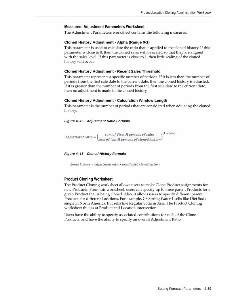
Product/Location Cloning Administration Workbook
Setting Forecast Parameters 4-39
Measures: Adjustment Parameters Worksheet The Adjustment Parameters worksheet contains the following measures:
Cloned History Adjustment - Alpha (Range 0-1)This parameter is used to calculate the ratio that is applied to the cloned history. If this parameter is close to 0, then the cloned sales will be scaled so that they are aligned with the sales level. If this parameter is close to 1, then little scaling of the cloned history will occur.
Cloned History Adjustment - Recent Sales ThresholdThis parameter represents a specific number of periods. If it is less than the number of periods from the first sale date to the current date, then the cloned history is adjusted. If it is greater than the number of periods from the first sale date to the current date, then no adjustment is made to the cloned history.
Cloned History Adjustment - Calculation Window LengthThis parameter is the number of periods that are considered when adjusting the cloned history.
Figure 4–15 Adjustment Ratio Formula
Figure 4–16 Cloned History Formula
Product Cloning WorksheetThe Product Cloning worksheet allows users to make Clone Product assignments for new Products. From this worksheet, users can specify up to three parent Products for a given Product that is being cloned. Also, it allows users to specify different parent Products for different Locations. For example, CS Spring Water 1 sells like Diet Soda single in North America, but sells like Regular Soda in Asia. The Product Cloning worksheet thus is at Product and Location intersection.
Users have the ability to specify associated contributions for each of the Clone Products, and have the ability to specify an overall Adjustment Ratio.

Product/Location Cloning Administration Workbook
4-40 Oracle Retail Demand Forecasting User Guide for the RPAS Classic Client
Figure 4–17 Product Cloning Worksheet
Measures: Product Cloning WorksheetThe Product Cloning worksheet contains the following measures:
Product ClonesProduct Clone1, Product Clone 3, Product Clone 3
Parent Products for the new Product being cloned. It is optional to specify more than one product clone. The selection or assignment of product clone is made by clicking this measure and a Single Hier Select wizard appears. Assignments are made by selecting a product and clicking OK. See the Oracle Retail Predictive Application Server User Guide for more details on the Single Hier Select wizard.

Product/Location Cloning Administration Workbook
Setting Forecast Parameters 4-41
Figure 4–18 Product Clone Selection
Product Clone ContributionsProduct Clone Contribution1, Product Clone Contribution2, Product Clone Contribution3
Relative contributions of all clone products. If user does not specify contributions, but makes selections for product clones and commits the changes, at the time of commit the contributions are calculated to have equal weights for all specified product clones. If user specifies Product clone contributions, they get normalized such that they add up to one at the time of commit. Product clone contributions with no associated product clone values get set to zero at the time of commit.
Clone Product Adjustment RatioYou may enter an Adjustment Ratio to apply to the cloned history of the new product. This is a real number between [0, infinity]. The default (NA) value is 1.00, (in other words 100%), which translates to no adjustment.
Example 4–2 Clone Product Adjustment Ratio
If demand for a new item is expected to be 30% greater than its clone item, the Adjustment Ratio would be set to 1.30. If demand for a new item is expected to be 30% less than its clone item, the Adjustment percent would set to 0.70.

Product/Location Cloning Administration Workbook
4-42 Oracle Retail Demand Forecasting User Guide for the RPAS Classic Client
Location Cloning WorksheetLocation Cloning worksheet allows users to make clone Location assignments for new Locations. Location Cloning worksheet allows users to specify up to three Clone Locations for a given Location that is being cloned. Also, it allows users to specify different parent Locations for different products. For example, the Beverly Hills store sells like the Miami store for swim wear and sells like the New York store for electronics. The Location Cloning worksheet thus is at Location and Product intersection.
Users have the ability to specify associated contributions for each of the Parent Locations, and have the ability to specify an overall Adjustment Ratio.
Figure 4–19 Location Cloning Worksheet
Measures: Location Cloning WorksheetThe Location Cloning worksheet contains the following measures:
Location ClonesLocation Clone1, Location Clone 3, Location Clone 3
Parent Locations for the new Location being cloned. It is optional to specify more than one parent clones. The selection or assignment of Location Clone is made by clicking this measure and a Single Hier Select wizard appears. Assignments are made by selecting a Location and clicking OK. See the Oracle Retail Predictive Application Server User Guide for more details on the Single Hier Select wizard.

Product/Location Cloning Administration Workbook
Setting Forecast Parameters 4-43
Figure 4–20 Select Location Clone
Location Clone ContributionsLocation Clone Contribution1, Location Clone Contribution2, Location Clone Contribution3
Relative contributions of all Clone Locations. If user does not specify contributions, but makes selections for Location Clones and commits the changes, at the time of commit the contributions are calculated to have equal weights for all specified Location Clones. If user specifies contributions, at the time of commit, Location clone contributions get normalized so that they add up to 1. Location Clone contributions with no associated Location Clone values get set to zero at the time of commit.
Clone Location Adjustment RatioYou may enter an Adjustment Ratio to apply to the cloned history of the new location. This is a real number between [0, infinity). The default (NA) value is 1.00, (in other words 100%), which translates to no adjustment.
Example 4–3 Clone Location Adjustment Ratio
If demand for a new store is expected to be 30% greater than its clone store, the Adjustment Ratio would be set to 1.30. If demand for a new store is expected to be 30% less than its clone store, the Adjustment percent would set to 0.70.
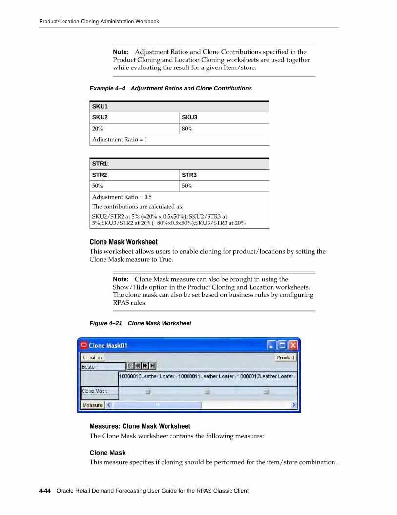
Product/Location Cloning Administration Workbook
4-44 Oracle Retail Demand Forecasting User Guide for the RPAS Classic Client
Example 4–4 Adjustment Ratios and Clone Contributions
Clone Mask WorksheetThis worksheet allows users to enable cloning for product/locations by setting the Clone Mask measure to True.
Figure 4–21 Clone Mask Worksheet
Measures: Clone Mask WorksheetThe Clone Mask worksheet contains the following measures:
Clone MaskThis measure specifies if cloning should be performed for the item/store combination.
Note: Adjustment Ratios and Clone Contributions specified in the Product Cloning and Location Cloning worksheets are used together while evaluating the result for a given Item/store.
SKU1
SKU2 SKU3
20% 80%
Adjustment Ratio = 1
STR1:
STR2 STR3
50% 50%
Adjustment Ratio = 0.5
The contributions are calculated as:
SKU2/STR2 at 5% (=20% x 0.5x50%); SKU2/STR3 at 5%;SKU3/STR2 at 20%(=80%x0.5x50%);SKU3/STR3 at 20%
Note: Clone Mask measure can also be brought in using the Show/Hide option in the Product Cloning and Location worksheets. The clone mask can also be set based on business rules by configuring RPAS rules.

5
Generating and Approving a Forecast 5-1
5Generating and Approving a Forecast
Once a user has completed setting all global and individual forecast parameters a forecast must be generated and approved. The Forecast workbook template group provides the workbooks necessary to support these tasks.
Refer to Appendix A, "Appendix: RDF Workbooks"for a complete list of RDF workbooks, and their respective tabs, worksheets, and measures.
Run a Batch Forecast The forecast generation process creates demand forecasts for all product/location combinations that are set to forecast within the forecast horizon window. Forecasts are typically run automatically as scheduled batch jobs. RDF regularly triggers a set of processes to be run at a pre-determined time when system use is at a minimum, such as overnight.
Scheduling of the automatic batch forecasting process is supported in part through the Forecast Administration Workbook where a default value is set for the forecast cycle (number of days between forecast runs). The Forecast Cycle measure and Next Run Date field in the Forecast Administration Workbook support the automatic scheduling of batch forecasting jobs in the RDF solution. Refer to the Forecast Administration Workbook description for further information.
Run Batch Forecast WorkbookThe Run Batch Forecast Workbook wizard allows you to manually execute the forecast generation process at a time other than the regularly scheduled batch job. If a global domain environment is implemented, forecasts generated in the Local domain can be viewed in the Master domain, however this forecast is isolated to the data in the Local domain. The execution of PreGenerateForecast at the Master domain, then passing the output of the process to Generate from the back-end of each Local domain allows for the Local domains to share a birth date, thus supporting a view to forecast data across Local domains in the Master domain. See the Oracle Retail Demand Forecasting Implementation Guide for more information on PreGenerateForecast and Generate.
Running a Batch Forecast ManuallyThe following sections describe the procedures to manually run a batch forecast.

Delete Forecasts
5-2 Oracle Retail Demand Forecasting User Guide for the RPAS Classic Client
Before You BeginPrior to using the Run Batch Forecast Workbook wizard, at minimum the following tasks must be performed:
1. Create or access a Forecast Administration Workbook.
2. In the Forecast Start Date measure, enter the starting date of the forecast horizon; otherwise the system defaults to the system date (today).
3. Set a Default Forecasting Method for the Final and Source Level.
4. Set a Default Source Level for the Final Level.
5. Set the Forecast Length if there is no value already in this measure.
6. Set the Spreading Profile if the Source Levels are at aggregate dimensions above the Final Level.
7. Commit any changes by selecting from the File menu, then select Commit Now.
8. Close the workbook.
ProcedureFollow these steps to manually run a batch forecast:
1. Within the Local or Simple domain, select New from the File menu.
2. Select the Forecast tab to display a list of workbook templates for statistical forecasting. Highlight Run Batch Forecast and click OK.
3. The Run Batch Forecast wizard opens and prompts you to select the Final Levels to forecast. Select Next or Finish.
The Run Batch wizard automatically executes PreGenerateForecast and Generate within the Simple or Local Domain. If Next is selected from the last wizard screen, the wizard does not advance to the completion message until the forecast has been generated. Depending on the amount of product/locations to be forecast and the forecast horizon, it may take a several minutes before the system advances to the final screen. When the forecast generation is completed, the wizard displays a screen that notifies you of the forecast generation ID.
After a forecast is generated, the Forecast Start Date field is cleared. This ensures that the same forecast is not generated again on the same date. The Next Run Date field is also updated based on the birth date of the forecast plus the Forecast Cycle. Both fields can be viewed in the Forecast Administration Workbook.
Delete ForecastsThe Days to Keep Forecasts parameter (set in the Forecast Administration Workbook) supports the automatic deletion of old forecasts when the Run Batch wizard or PreGenerateForecast is executed. Occasionally, a user may need to manually delete a forecast. Some reasons might include:
■ A forecast was run with the wrong source levels selected.
■ The forecast horizon was not properly set.
■ Old forecasts need to be deleted to save space on the server.
The Delete Forecasts wizard guides you through the process of deleting unwanted forecasts from the system. Deletions of forecasts are permanent.

Delete Forecasts
Generating and Approving a Forecast 5-3
Forecast Delete Workbook
If the Forecast Delete wizard is used in a global domain environment, deleting a forecast in the Master domain deletes the selected birth date within all domains. Deleting a forecast in the Local domain deletes the selected birth date only within the Local domain.
1. From the Simple domain, Master domain, or Local domain; select New from the File menu.
2. Select the Forecast tab to display a list of workbook templates for demand forecasting.
3. Select Forecast Delete.
4. Click OK.
5. Select the forecast generation dates of the forecast to delete.
Figure 5–1 Forecast Delete Wizard
6. Click Next.
7. Select Yes to verify forecast deletion, or No to cancel deletion and exit the Forecast Delete wizard.
8. Click Finish to process the request. If Yes was selected on the final wizard screen, the forecast is deleted.
Note: The deletion of forecasts from RDF is permanent.

Forecast Approval Workbook
5-4 Oracle Retail Demand Forecasting User Guide for the RPAS Classic Client
Forecast Approval WorkbookAfter the forecast is generated, the next steps in the forecasting process are analysis and approval. Approval of forecasts is required before the forecast data can be exported to other processes, such as replenishment programs. The Forecast Approval workbook allows you to view, analyze, adjust, and approve forecast results.
Some system forecasts may be set to be automatically approved by the system. The default approval method for items in a forecast is set in the Forecast Administration Workbook, and these policies can be amended for individual product/location combinations in the Forecast Maintenance Workbook. Any forecasts not set to Automatic Approval may require evaluation, adjustments, and ultimately approval before subsequent processes are executed.
You can view and analyze forecast data at multiple forecast levels (source level and final level) simultaneously. Revisions to and approvals of final level forecast values are made on the appropriate worksheets in the Forecast Approval workbook. The Forecast Approval workbook can contain these worksheets:
When the Forecast Approval workbook is displayed, you may review the system-generated forecast and measures for any levels included in the workbook and make adjustments to forecast values at the final level. Forecast values are overwritten in the Adjusted Forecast measure on the Final Forecast worksheet. Approvals are made for each product/location combination in the Approval Method measure of the Forecast Approval worksheet.
After you complete your work, you can save the workbook using the Save function on the File menu. To update the master database with the approved forecast values, you must commit the workbook using the Commit Now or Commit Later option on the File menu. Once the workbook is committed, the forecast values are stored in the master database and can be used by other processes.
Worksheet Description
Final Forecast worksheet
This worksheet allows you to review final level system-forecast quantities and make revisions to them if needed.
Source Level worksheet
This worksheet displays the system-generated source level forecast, and allows you to compare this data with final level forecast values.
Approval worksheet This worksheet allows you to specify the manual approval policy of forecasts by product and location.
Final System Parameters worksheet
This option is only available if Generate System Parameters or Generate Methods is turned on in the Forecast Administration Workbook.
Source System Parameters worksheets
This option is only available if Generate System Parameters or Generate Methods is turned on in the Forecast Administration Workbook, and a Source Level was designated in Forecast Administration.
Valid Forecast Run worksheet
This worksheet allows you to review the partition dimensions in which the generated forecast was run.

Forecast Approval Workbook
Generating and Approving a Forecast 5-5
Opening or Creating the Forecast Approval WorkbookSelect Open from the File menu to bypass the Forecast Approval wizard and open an existing Forecast Approval workbook or perform the following:
1. Within the Master domain, Simple domain, or Local Domain; select New from the File menu.
2. Select the Forecast tab to display a list of workbook templates for statistical forecasting.
3. Select Forecast Approval. Click OK.
4. The Forecast Approval wizard opens and prompts you to select the final level at which to approve forecast values. Make your selection and click Next.
5. Select the forecast levels to include in the Forecast Approval workbook. Select as many forecast levels as necessary for comparison. Click Next.
6. Select the birth date of the forecast you wish to approve.
■ Select Use the most recently generated forecast to build a workbook containing the most recent forecast values.
■ Click Select from a list of forecast to select from a list of previously generated forecasts stored in the system. Note that if this option is selected, the system automatically highlights the first forecast in the list, and if no further selections are made by you, this first forecast is used.
■ If no selection is made by you, the birth date defaults to the latest generated generation ID. Click Next.
7. Select the specific locations you want to view. It is important to include all locations that are members of the location dimensions in the forecast levels to be analyzed. For example, if you select to view a forecast level that is defined at item/chain/week, you should include all locations that are members of the particular chain to be analyzed. It is recommended that Position Query functionality or selection from aggregate levels in the Location hierarchy is employed if the workbook is generated using AutoWorkbook build. Click Next.
8. Select the merchandise you want to view. It is important to include all products that are members of the Merchandise dimensions in the forecast levels to be analyzed. For example, if you select to view a forecast level that is defined at subclass/store/week, you must include all items that are members of the particular subclass to be analyzed. It is recommended that Position Query functionality or selection from aggregate levels in the Merchandise hierarchy is employed if the workbook is generated using AutoWorkbook build. Click Next.
9. Select the first date of history to include in the workbook. You may choose to either set the Forecast Start Date minus the number of periods or select the first date of history from the displayed list. It is recommended that the Forecast Start Date minus the number of periods is set if the workbook is generated using AutoWorkbook build. Click Next.
Note: Use the most recently generated forecast must be selected if the workbook supports an AutoWorkbook build.

Forecast Approval Workbook
5-6 Oracle Retail Demand Forecasting User Guide for the RPAS Classic Client
10. Select the last date in the forecast horizon to include in the workbook. You may either choose to Include the following number of time periods of the forecast horizon or select the last date to include of the horizon from the displayed list. It is recommended that Include the following number of time periods of the forecast horizon is set if the workbook is generated using AutoWorkbook build. The value entered must be within the forecast horizon. Click Next.
11. Select the last date in the calendar to include in the workbook. You may choose to either set the Forecast end date plus the following number of time periods or select the last date to include of the post-horizon calendar from the displayed list. It is recommended that Forecast end date plus the following number of time periods is set if the workbook is generated using AutoWorkbook build. Click Next.
12. Place check marks next to any additional registered measures you would like to view in your workbook. The valid values of these measures may only be viewed if Generate Intervals, Generate Cumulative Intervals, Generate Methods, Generate Parameters, Generate Baselines, or Store Interim Forecasts were selected in the Forecast Administration Workbook. Click Next.
13. From the list provided, select any additional measures beyond the default measures in the workbook that you would like to view. Click Finish to build and open the workbook.
Window Descriptions for the Forecast Approval WorkbookThe following sections describe the components of the Forecast Approval workbook.
Final Level WorksheetThe Final Level worksheet allows you to review the forecast quantities and make adjustments to forecasts if needed. The primary objective in the Forecast Approval workbook is to review and edit forecast values using the Adjusted Forecast field on the Final Level worksheet and, ultimately approve forecasts that have been user-adjusted or require manual approval.
Note: If you make no selection, the system uses the forecast start date.
Note: If you make no selection, the system uses the last date in the forecast horizon chosen by you in the previous wizard screen.
Note: If any of these parameters are included in the Forecast Approval workbook using AutoWorkbook build and are later deselected for generation in the Forecast Administration Workbook, AutoWorkbook must be set again.

Forecast Approval Workbook
Generating and Approving a Forecast 5-7
Figure 5–2 Final Level Worksheet
Measures: Final Level WorksheetThe Final Level worksheet contains the following measures:
Adjusted Cumulative IntervalWhen changes are made to the Adjusted Forecast, the value of the Forecast Cumulative Interval is recalculated in this measure. The values in this measure are read-only. To view and store this measure:
■ Generate Cumulative Intervals must be selected in the Forecast Administration Workbook.
■ Cumulative Intervals must be selected to be viewed in the Forecast Approval wizard.
Adjusted ForecastThe value in this field initially defaults to the System Forecast if the forecast is automatically approved by the system or through a Forecast Approval Alert. Otherwise, the value in the Adjusted Forecast is different than the System Forecast if:
■ Adjusted Forecast has been updated by you.
■ Keep Last Changes is set to Total, Difference or Ratio.
■ Update Last Weeks Forecast is set to Replicate.
Changes to the Adjusted Forecast is automatically approved. The Approval worksheet updates with the date of the adjustment and the name of the user who made the adjustment.
Note: Changes to the Adjusted Forecast for periods outside of the forecast horizon are not committed.
Edits to any non-committed values in the Forecast Approval Workbook are overwritten when data is refreshed.

Forecast Approval Workbook
5-8 Oracle Retail Demand Forecasting User Guide for the RPAS Classic Client
Approved Cumulative IntervalThe Approved Cumulative Interval is the cumulative interval that was approved at the time of the workbook build. The values contained in this measure are read-only. If changes are made to the Adjusted Forecast, the Approved Cumulative Interval reflects the recalculated values when the workbook is committed and data is refreshed.
Approved ForecastThe Approved Forecast is the forecast quantity that was approved at the time of the workbook build. The values contained in this measure are read-only. If changes are made to the Adjusted Forecast, then click Calculate to show the new value in the Approved Forecast.
Approved System ForecastThe Approved System Forecast is populated with the last System Forecast approved for a time series:
1. Approval Method set to Automatic Approval
2. Approval Method set to a Forecast Approval Alert and the alert is not triggered
3. Update Last Weeks Forecast is set to Use Forecast
The values in this measure are read-only.
Forecast Cumulative IntervalCumulative Intervals are used in safety stock calculation within allocation and replenishment systems. This value is similar to a running total of the Forecast Interval and is read-only. To see this measure:
■ Generate Cumulative Intervals must be selected in the Forecast Administration Workbook.
■ Cumulative Intervals must be selected to be viewed in the Forecast Approval wizard.
Forecast IntervalThe Forecast Interval is calculated on the particular forecast region as capped standard deviation for some methods. It takes into consideration the system forecast for capping as well.
The forecast interval for any given week i is capped to a maximum of Forecast(i) * upperCapRatio. This cap is applied once the interval exceeds the system forecast, and it is applied for every value of the interval after that. The upperCapRatio (Interval Cap Upper Ratio) is a parameter set in the Forecast Administration Workbook.
The forecast interval is capped to a minimum of Forecast(i) * lowerCapRatio whenever the interval is less than this quantity. The lowerCapRatio (Interval Cap Lower Ratio) is another parameter set in the Forecast Administration Workbook.
When forecasts are approved, the corresponding Intervals and Cumulative Interval measures are approved. To see this measure:
■ Generate Intervals must be selected in the Forecast Administration Workbook.
■ Intervals must be selected to be viewed in the Forecast Approval wizard.

Forecast Approval Workbook
Generating and Approving a Forecast 5-9
History DataHistory Data (a read-only measure) is the sales data used to generate the forecast. This allows you to compare Actuals to forecast values. When the workbook is created, the Data Source measure is copied into History Data.
Interim ForecastThe Interim Forecast is the forecast generated at the final level that is used as the Data Source in Curve to produce the Spreading Profile. This profile determines how the Source Forecast is spread down to the Final Forecast level. The values in this measure are read-only. To see this measure:
■ Generate Interim Forecast must be selected in the Forecast Administration Workbook.
■ Interim Forecast must be selected to be viewed in the Forecast Approval wizard.
Last Approved ForecastThe Last Approved Forecast is the approved system forecast value when an approval occurred on a previous batch forecast for the time series. The values contained in this measure are read-only.
System BaselineThe System Baseline is a forecast generated on past sales data that contains no promotions (that is, normal demand given no causal effects). To see a generated Baseline Forecast:
■ Promotional Forecasting must be implemented.
■ Generate Baseline must be selected in the Forecast Administration Workbook.
■ The System Baseline must be selected to be viewed in the Forecast Approval wizard.
System ForecastThe System Forecast displays the system generated forecast for the time series. The values contained in this field are read-only. This measure includes baseline as well as promotional lifts and regular price lifts, if applicable.
System Forecast without Regular Price LiftThe System Forecast without Regular Price Lift displays the system generated forecast without regular price lifts applied.
Regular PriceThe Regular Price measure displays the regular price plan.
Regular Price Halo Lift The Regular Price Halo Lift displays the halo lift (in units) resulting from a regular price change. It is applied additively on top of the System Forecast without Regular Price Lift, together with the other regular price lifts, to calculate the System Forecast.
Regular Price Halo Lift RatioThe Regular Price Halo Lift Ratio displays the halo lift (as a ratio) resulting from a regular price change. It is applied multiplicatively on top of the System Forecast without Regular Price Lift, together with the other regular price lifts, to calculate the System Forecast.

Forecast Approval Workbook
5-10 Oracle Retail Demand Forecasting User Guide for the RPAS Classic Client
Regular Price Cannibalization LiftThe Regular Price Cannibalization Lift displays the cannibalization lift (in unit) resulting from a regular price change. It is applied additively on top of the System Forecast without Regular Price Lift, together with the other regular price lifts, to calculate the System Forecast.
Regular Price Cannibalization Lift RatioThe Regular Price Cannibalization Lift Ratio displays the cannibalization lift (as a ratio) resulting from a regular price change. It is applied multiplicatively on top of the System Forecast without Regular Price Lift, together with the other regular price lifts, to calculate the System Forecast
Regular Price Self LiftThe Regular Price Self Lift displays the self lift (in units) resulting from a regular price change. It is applied additively on top of the System Forecast without Regular Price Lift, together with the other regular price lifts, to calculate the System Forecast.
Regular Price Self Lift RatioThe Regular Price Self Lift Ratio displays the self lift (as a ratio) resulting from a regular price change. It is applied multiplicatively on top of the System Forecast without Regular Price Lift, together with the other regular price lifts, to calculate the System Forecast.
Source Level WorksheetThe Source Level worksheet displays the system-generated source level forecast. Final level forecast values in the Final Level worksheet can be viewed alongside and compared with their corresponding source level forecasts.
Figure 5–3 Source Level Worksheet
Measures: Source Level WorksheetThe Source Level worksheet contains the following measures:
History DataHistory Data (a read-only measure) is the sales data used to generate the forecast. This allows you to compare Actuals to forecast values. When the workbook is created, the Data Source measure is copied into History Data.

Forecast Approval Workbook
Generating and Approving a Forecast 5-11
System BaselineThe System Baseline is a forecast generated on past sales data that contains no promotions (that is, normal demand given no causal effects). To see a generated Baseline Forecast:
■ Promote must be implemented.
■ Generate Baseline must be selected in the Forecast Administration Workbook.
■ The System Baseline must be selected to be viewed in the Forecast Approval wizard.
System ForecastThe System Forecast displays the system generated forecast for the time series. The values contained in this field are read-only.
Approval WorksheetThe Forecast Approval worksheet allows for non-adjusted System Forecast to be approved. This worksheet can also be used to view the approval date of forecast values, and also display the name of the user that manually approved forecast values for a given product/location combination. The default Approval Method is set in Forecast Administration Workbook and for product/location combinations that vary from the default, the Forecast Maintenance Workbook can be used.
Figure 5–4 Approval Worksheet
Measures: Approval WorksheetThe Approval worksheet contains the following measures:
Approval CommentApproval Comment is a field in which notes may be entered regarding the forecast values or any pertinent information for specified product/location combinations.
Approval DateApproval Date is a read-only field that displays the date that the forecast quantity was approved either automatically during the batch forecast process or when changes are made to the Adjusted Forecast. This information is necessary for RDF to carry out any subsequent processes, such as replenishment procedures.

Forecast Approval Workbook
5-12 Oracle Retail Demand Forecasting User Guide for the RPAS Classic Client
Approved ByApproved By is a read-only field that displays the name of the user to approve forecasts for an item/location. This field may be populated with Sys if the system was set to automatically approve forecasts during the batch forecast process.
Manually ApprovedManually Approved is a Boolean flag. This field may be checked if you want to accept the System Forecast quantity for a time series that has yet to be approved. The flag is also activated when a change is made to the Adjusted Forecast and Calculate occurs. When this flag is activated, the time series for an item/location are approved and both the Approval Date and Approved By fields are updated.
Final or Source System Parameters WorksheetThe Final or Source Parameters worksheets allow you to view the alpha, level, and trend parameters for each fitted time series. These parameters are only available to be viewed if Generate Parameters or Generate Methods are activated in the Advanced tab of the Forecast Administration Workbook.
Figure 5–5 System Parameters Worksheet
Measures: Final or Source System Parameters WorksheetThe Final or Source Parameters worksheet contains the following measures:
Forecast Method PickedThis is the system-calculated alpha value (which is an internal optimization parameter that corresponds to the rate of decay of the weighting on the historical values) for the corresponding product/location combination if the chosen method is one of the following methods: Simple, Holt, Additive Winters, Multiplicative Winters, and Profile Based. To see this measure:
■ Generate Parameters must be selected in the Forecast Administration Workbook.
■ System Generated Parameters must be selected to be viewed in the Forecast Approval wizard.
System Generated AlphaThis is the system-calculated alpha value (which is an internal optimization parameter that corresponds to the rate of decay of the weighting on the historical values) for the corresponding product/location combination if the chosen method is one of the following methods: Simple, Holt, Additive Winters, Multiplicative Winters, and Profile Based.

Forecast Approval Workbook
Generating and Approving a Forecast 5-13
To see this measure:
■ Generate Parameters must be selected in the Forecast Administration Workbook.
■ System Generated Parameters must be selected to be viewed in the Forecast Approval wizard.
System Generated LevelThis is the system-calculated level (which is the constant baseline forecast) if the chosen method is one of the following methods: Simple, Holt, Additive Winters, Multiplicative Winters, and Seasonal Regression. To see this measure:
■ Generate Parameters must be selected in the Forecast Administration Workbook.
■ System Generated Parameters must be selected to be viewed in the Forecast Approval wizard.
System Generated TrendThis is the system-calculated trend (which is the rate of change of the baseline forecast with time) if the chosen method is one of the following methods: Holt, Additive Winters, Multiplicative Winters, and Seasonal Regression. To see this measure:
■ Generate Parameters must be selected in the Forecast Administration Workbook.
■ System Generated Parameters must be selected to be viewed in the Forecast Approval wizard.
Valid Forecast Run WorksheetIn a global domain environment, the Valid Forecast Run worksheet allows you to identify which Local domains share the forecast birth date selected in the wizard when viewed in the Master domain. If in a Local domain, only the single position of the partition dimension is displayed.
Figure 5–6 Valid Forecast Run Worksheet
Measures: Valid Forecast Run WorksheetThe measure displayed on this worksheet is viewed at final level/partition intersection. The Valid Forecast Run worksheet includes the following standard measure:

Approving Forecasts Through Alerts (Exception Management)
5-14 Oracle Retail Demand Forecasting User Guide for the RPAS Classic Client
Final Level Run FlagThe Final Level Run Flag is a read-only Boolean measure. A check (set to True) displayed in this field indicates which positions from the partition dimension had a successful forecast run for the birth date selected in the Forecast Approval wizard.
Approving Forecasts Through Alerts (Exception Management)RDF provides you with ability to manually approve every product/location forecast value. However, due to the extremely large volume of product/location forecast values that is generated for each forecast cycle, RPAS provides additional functionality that enhances your ability to evaluate and approve a forecast.
When configuring an RDF solution, specific Forecast Approval Alerts and alert parameters may be defined and applied during the batch process, and they may also be inserted into the Forecast Approval Workbook. Alerts report product/location forecast values that exceed expected thresholds. If a specific product/location forecast value exceeds a threshold, the alert measure is flagged as on and visible to you as a check mark in the appropriate product/location intersection.
The complexities of retail operations can result in the need to define many alerts; each designed to watch for a specific scenario that would require a user's evaluation of a forecast value.
For more information on how alert measures and rules are defined and registered, refer to the Oracle Predictive Application Server Configuration Tools User Guide and Oracle Retail Demand Forecasting Implementation Guide.
Note: Edits to the Adjusted Forecast can only be committed for partitions that have an activated Final Level Run Flag.

6
Forecast Analysis Tools 6-1
6Forecast Analysis Tools
RDF provides you with a number of tools that may be used for additional forecast analysis. The Forecast workbook template group provides the workbooks necessary to complete these tasks.
Refer to Appendix A, "Appendix: RDF Workbooks" for a complete list of RDF workbooks, and their respective tabs, worksheets, and measures.
Interactive Forecasting WorkbookThe Interactive Forecasting workbook is a forecast simulation tool that allows you to make changes to forecast parameters and see the results without having to wait for the batch run. In this workbook, you can edit various forecast parameters including sales history and forecast method. A new forecast is produced based on the changed parameters. In addition to forecasts, the Interactive Forecasting workbook can also generate fit in historical region and the system picked model if an ES forecast method is used.
Opening the Interactive Forecasting WorkbookUse the following procedure to open the Interactive Forecasting workbook.
1. Within the Local or Simple domain, select New from the File menu.
2. Select the Forecast tab to display a list of workbook templates.
3. Select Interactive Forecasting. Click OK.
4. Select the forecast level. Click Next.
5. Select the forecast starting date. Click Next.
6. Select the first date in the historical data to use for generating the forecast. Click Next.
7. Select the end date for the forecast horizon. Click Next.
8. Perform one of the following options:
■ Specify future time periods beyond the forecast horizon to include in your workbook.
■ Select Do not include dates after the horizon if no future dates are to be included in the workbook.
9. Click Next.
10. Select the products to be included in the workbook. Click Next.

Interactive Forecasting Workbook
6-2 Oracle Retail Demand Forecasting User Guide for the RPAS Classic Client
11. Select the locations to be included in the workbook. Click Next.
12. Select extra measures (if needed) to be included in the forecasting workbook.Click Finish.
Once the wizard is completed, the forecast is generated based on your selections in the wizard and the Default Forecast Method set for the specified forecast level in the Forecast Administration Workbook.
After the forecast generation is complete, the Interactive Forecasting workbook is displayed.
The workbook contains two worksheets:
■ Forecasting Parameter Worksheet
■ Interactive Forecasting Worksheet
Window Descriptions for the Interactive Forecasting WorkbookThe following sections describe the components of the Interactive Forecasting workbook.
Forecasting Parameter WorksheetThe Forecasting Parameter worksheet is based on the intersection of the Product and Location dimensions for the select forecast level.
The Forecasting Parameter worksheet contains the following measures. Of these measures, all but System picked model are editable. Changes can be made to the editable parameters, that is, History Start Date, Forecast Method, Forecast Start Date, and Forecast End Date to regenerate a forecast of the time series.
Figure 6–1 Forecast Parameter Worksheet
Measures: Forecasting Parameter WorksheetThe Forecasting Parameter worksheet contains the following measures:
Forecast MethodA list from which you can select the method used to generate the forecast. The workbook defaults to the method selected in the Forecast Administration Workbook for the specified level if the method is supported by Interactive Forecasting. Otherwise, it defaults to No Forecast.

Interactive Forecasting Workbook
Forecast Analysis Tools 6-3
Forecast Picked MethodThis is the method that was used to generate the forecast for the given product/location combination. This field is useful when combined methods are requested (for example ES methods). Then this field displays the actual method the system picked from the combined methods. In case stand-alone methods are chosen, generally this field is the same as the method chosen in Forecast Administration or Forecast Maintenance. However, if the requested method is unable to produce a good fit, the system defaults to a simpler method and that method is displayed here.
History Start DateThis is the starting date for historical sales data. For example, if your system start date is January 1, 2003, but you only want to use historical sales data from the beginning of 1999, you need to set your History Start Date to January 1, 1999. Only history after this date is used for generating the forecast. The default is the system start date unless otherwise specified. If sales data is collected weekly or monthly, RDF generates forecasts only using data from sales periods after the one containing the history start date.
It is also important to note that the system ignores leading zeros that begin at the history start date. For example, if your history start date is January 1, 1999, and an item/location does not have sales history until February 1, 1999, the system considers the starting point in that item/location's history to be the first data point where there is a non-zero sales value.
Forecast Start DateThis is first date of the forecast horizon. The default is the start date selected in the wizard.
Forecast End DateThis is the last date of the forecast horizon. The default is the end date selected in the wizard.
Additional Information about the Interactive Forecasting Workbook ParametersInteractive Forecasting assumes that the historical data are contained in the measure posxlxb. All forecasts generated by interactive forecasting are based on these data.
Performance may be improved by utilizing a mask measure. Interactive forecasting uses the measures mask<forecast level>xb; for example mask01xb. Here, <forecast level> corresponds to the forecast level chosen in the wizard when opening the Interactive Forecasting workbook. The mask is a boolean measure. Only cells with value true are included in the forecast. This is useful when desiring to focus on only a few product/locations.
The Interactive Forecast method is intended to be a quick way to view results produced by different forecast methods. It allows the user to gauge, in a qualitative way, the suitability of a particular forecast method for a given set of sales history data. Even though it uses the exact same forecast methods as the full forecast, only the parameters listed previously will affect the results. No other user-input values are used. Users wishing to vary a larger number of parameters are encouraged to use the regular forecast functionality.

Forecast Scorecard Workbook
6-4 Oracle Retail Demand Forecasting User Guide for the RPAS Classic Client
Interactive Forecasting WorksheetThe Interactive Forecasting worksheet is based on the intersection of the Product, Location, and Calendar dimensions for the forecast level selected in the wizard process. The Interactive Forecasting worksheet contains the History Data and the System Forecast. Of these measures, only History Data is editable.
Figure 6–2 Interactive Forecasting Worksheet
Measures: Interactive Forecasting WorksheetThe Interactive Forecasting worksheet contains the following measures:
History DataThis is the historical sales data set in the Forecast Administration Workbook. This field is editable so you can change out-of-character sales if needed. For example, if your battery sales went up during a major power outage, you can lower the sales data back to a more normal level so the unusually high sales adversely affects your forecast. However these changes are for simulation purposes only and cannot be committed.
System ForecastThe quantity that the system predicts is required for the product, location, and calendar combination displayed. Changes to History Data, History Start Date, Forecast Start Date, Forecast End Date, and Forecast Method causes the System Forecast to re-calculate when Calculate is selected from the toolbar.
Forecast Scorecard WorkbookThis section describes the purpose and content of the Forecast Scorecard and the steps required in order to create and access this workbook. This section also discusses the two types of worksheets contained in the Forecast Scorecard workbook, as well as the definitions of parameters that exist in each. Evaluating forecast accuracy through the use of error statistics is discussed, as is the process of comparing historical forecasts to actual sales data.
The purpose of the Forecast Scorecard is to monitor the accuracy of both system-generated forecasts and approved final forecasts. Once a forecast has been generated and actual point-of-sale data is received for the forecast period, statistical information can be reviewed to help you analyze the accuracy of forecasting models and methods.
The Forecast Scorecard template consists of a wizard and two worksheets.

Forecast Scorecard Workbook
Forecast Analysis Tools 6-5
Based on your selections in the wizard, the Forecast Scorecard provides statistical information and comparison data that allow you to monitor the accuracy of system-generated forecasts and final approved forecasts.
■ The Final Error Measure worksheet displays statistical information, such as mean error and root mean squared error, that reflects the accuracy of the forecast.
■ The Final Actuals versus Forecasts worksheet displays forecast results and actual point-of-sale values for specified product/location/calendar combinations.
Opening or Creating a Forecast Scorecard WorkbookSelect Open from the File menu to bypass the Forecast Scorecard wizard. Or, perform the following:
1. Within the Master, Local or Simple domain, select New from the File menu.
2. Select the Forecast tab to display a list of workbook templates.
3. Select Forecast Scorecard. Click OK. The Forecast Scorecard wizard opens.
4. You are prompted to select the forecast level that you want to evaluate. Make a selection. Click Next.
5. Select the generation date of the forecast you wish to review:
■ Click Use the most recent generated forecast to build a workbook containing the most recent forecast values.
■ Click Select from a list of forecast to select from a list of previously generated forecasts stored in the system.
6. Click Next.
7. Select the measures associated with the forecast results to be evaluated. Click Next.
8. Check the boxes corresponding to the error statistics that you want calculated for the forecast data. Click Next.
9. Select the specific locations that you want to view. It is important to include all locations that are members of the location dimensions in the forecast levels to be analyzed. For example, if you select to view a forecast level that is defined at item/chain/week, you should include all locations that are members of the particular chain to be analyzed. It is recommended that Position Query functionality or selection from aggregate levels in the location hierarchy is employed if the workbook supports an AutoWorkbook build. Make your selection. Click Next.
10. Select the merchandise you want to view. It is important to include all products that are members of the Merchandise dimensions in the forecast levels to be analyzed. For example, if you select to view a forecast level that is defined at subclass/store/week, you must include all items that are members of the particular subclass to be analyzed. It is recommended that Position Query functionality or selection from aggregate levels in the Merchandise hierarchy is employed if the workbook supports an AutoWorkbook build. Make your selection. Click Next.
11. Select the first date of history to include in the workbook. You may either choose to set the Forecast Start Date minus the number of periods or select the first date of history from the displayed list. It is recommended that the Forecast Start Date minus the number of periods is set if the workbook supports an AutoWorkbook build. Make your selection. Click Next.

Forecast Scorecard Workbook
6-6 Oracle Retail Demand Forecasting User Guide for the RPAS Classic Client
12. Select the last date in the forecast horizon to include in the workbook.
■ Choose Include the following number of time periods of the forecast horizon.
■ Select the last date to include of the horizon from the displayed list.
13. Click Next.
14. Select the last date in the calendar to include in the workbook.
■ Set the Forecast end date plus the following number of time periods.
■ Select the last date to include of the post-horizon calendar from the displayed list.
15. Click Next.
16. Select any additional measures to be included in the workbook. Click Finish.
The Forecasting workbook displays after the wizard process is completed.
Window Descriptions for the Forecast Scorecard WorkbookThe following sections describe the components of the Forecast Scorecard workbook.
Error Measure WorksheetThe Final Error Measure worksheet displays statistical information that reflects the accuracy of the forecast measures selected in the wizard process. You may need to evaluate a variety of such statistics to verify and compare forecast accuracy.
Given the situation, different levels of forecast accuracy can be useful. For example, in a situation with noisy data and no forecast previously available, a 200% error can be considered excellent and useful. In another situation with smooth data, if an old method of forecasting provided forecasts with a 10% error, a new method of forecasting with a 20% error would not be considered useful.
Different levels of forecasting accuracy are obtained at different levels of product aggregation. Item level forecasts with a 200% error can roll up into division-level forecasts with a 10% error. Therefore, the error measures are most useful when comparing different methods of forecasting or when looking at a particular model's accuracy over time. Accurate forecasts should lead to a reduction in inventory holding costs, or to an increase in customer service levels; forecast errors should be converted into dollars saved.
Note: It is recommended that Include the following number of time periods of the forecast horizon is set if the workbook supports an AutoWorkbook build.
Note: It is recommended that Forecast end date plus the following number of time periods is set if the workbook supports an AutoWorkbook build.
Note: All error statistics are calculated over the first period in the forecast to the last period in the forecast for which forecast data is available.

Forecast Scorecard Workbook
Forecast Analysis Tools 6-7
Figure 6–3 Error Measure Worksheet
Measures: Error Measure WorksheetThe Error Measure worksheet contains the following measures:
History Data for Forecast WindowThe sum of all actual sales from the first period in the forecast to the last period in the forecast for which point-of-sale data is available.
Forecast MeasuresYour workbook may include one or all of the forecast measures: System Forecast, Adjusted Forecast, Approved Forecast, Approved System Forecast, Interim Forecast. These measures are selected in the wizard process. This is the average value of these measures over the forecast horizon select in the wizard process.
Mean ErrorThe error of a forecast observation is the difference between the forecast value and the actual POS value. The Mean Error statistic is a measure of the average error over time. This is calculated by summing the errors for all observations, and then by dividing by the number of observations to obtain the average. It measures forecast accuracy by calculating the error in units. Because a positive error in one period can cancel out a negative error in another period, this measure is useful when you are interested in how well the forecast predicts over the forecast horizon rather than on a period-to-period basis. Mean error is useful as a measure of forecast bias. A negative mean error suggests that overall the forecasting model overstates the forecast while a positive mean error indicates forecasts that are generally too low.
Mean Absolute ErrorThe absolute error of a forecast observation is the absolute value of the difference between the forecast value and the actual POS value. The Mean Absolute Error statistic is a measure of the average absolute error. This is calculated by summing the absolute errors for all observations, and then by dividing by the number of observations to obtain the average. Mean Absolute Error gives you a better indication of how the forecast performed period by period, because the absolute value function ensures that negative errors in one period are not canceled out by positive errors in another. Mean Absolute Error is most useful for comparing two forecast methods for the same series.

Forecast Scorecard Workbook
6-8 Oracle Retail Demand Forecasting User Guide for the RPAS Classic Client
Root Mean Squared ErrorThis is the square root of the Mean Squared Error. The Root Mean Squared Error is one of the most commonly used measures of forecast accuracy because of its similarity to the basic statistical concept of a standard deviation. It evaluates the magnitude of errors in a forecast on a period-by-period basis, and it is best used to compare alternative forecasting models for a given series.
Mean Absolute Percentage ErrorThe percentage error of a forecast observation is the difference between the actual POS value and the forecast value, divided by the actual POS value. The result of this calculation expresses the forecast error as a percentage of the actual value. The Mean Absolute Percentage Error statistic measures forecast accuracy by taking the average of the sum of the absolute values of the percentage error calculations across all observations. This method is useful when comparing the accuracy of forecasts for different volume products (it normalizes error by volume).
Percentage Absolute ErrorThe absolute error of a forecast observation is the absolute value of the difference between the forecast value and the actual POS value. The Percentage Absolute Error statistic measures forecast accuracy by calculating the total absolute error as a percentage of the total actual POS. It is calculated by summing the absolute errors for all observations, dividing this value by the absolute value of the sum of all Actuals, and dividing the result by the number of observations in the series. Finally, multiply the total by 100 to obtain a percentage result.
Actuals versus Forecasts WorksheetThis worksheet displays forecast results and actual point-of-sale values for each product, location, and time period specified in the Forecast Scorecard wizard. This worksheet allows you to compare the results of both system-generated forecasts and final approved forecasts to actual sales quantities.
Figure 6–4 Actuals versus Forecast Worksheet
The Actuals versus Forecasts worksheet may contain the following measures:
Actuals These Actuals do not include: System Forecast, Adjusted Forecast, Approved Forecast, Approved System Forecast, Interim Forecast.

Forecast Scorecard Workbook
Forecast Analysis Tools 6-9
This displays the difference between the actual sales quantities and the committed forecast values for the forecast measures selected during the wizard process. Negative values indicate that the final forecast exceeded actual sales.
History DataHistory Data displays the actual point-of-sale quantities for the product, location, and calendar combinations displayed.
Forecast MeasuresYour workbook may include one or all of these forecast measures: System Forecast, Adjusted Forecast, Approved Forecast, Approved System Forecast, Interim Forecast. These measures are selected in the wizard process. These measures display the forecast quantity for the product, location, and calendar combinations included in the workbook.

Forecast Scorecard Workbook
6-10 Oracle Retail Demand Forecasting User Guide for the RPAS Classic Client

7
Promote (Promotional Forecasting) 7-1
7Promote (Promotional Forecasting)
This chapter provides an introduction to promotional forecasting and explains how it differs from the traditional statistical forecasting methodology. It discusses the advantages and limitations of both statistical and promotional forecasting models, and it outlines the use of Oracle Retail's Causal method of forecasting demand. It describes terminology used in the context of promotional forecasting, and it concludes with detailed descriptions of the workbook templates contained in the Promote workbook Template Group.
Refer to Appendix A, "Appendix: RDF Workbooks"for a complete list of RDF workbooks, and their respective tabs, worksheets, and measures.
Overview Promote is an optional add-on automated predictive solution that allows you to incorporate the effects of promotional and causal events (such as, radio advertisements and holiday occurrences) into your time-series forecasts. The promotional forecasting process uses both past sales data and promotional information to forecast future demand.
What Is Promotional Forecasting?Traditional statistical forecasting methods provide significant benefits to the process of forecasting consumer demand, because they are good at predicting level, trend, and seasonality based on sales history. The limitation of traditional statistical methods is that they forecast with less accuracy when there are special events that cause significant deviations in selling patterns.
For example, the Easter holiday, for which companies often run promotions, occurs on a different date each year. Traditional statistical forecast methods can identify seasonality in sales history, but this seasonality is based on periodic similarities in the sales pattern. Since Easter occurs on different dates from year to year (that is, its period of recurrence is not regular), manual intervention is required to predict change in demand using the traditional statistical forecasting method. Events like this are called promotion events. Promotion events, such as advertisements, irregularly occurring holidays, competitor information, free gift with purchase offers, and so on are events that drive businesses from the normal selling cycle.

Overview
7-2 Oracle Retail Demand Forecasting User Guide for the RPAS Classic Client
The goal of a promotional forecasting system is to improve time series forecasting by:
■ Providing the forecasting system with visibility as to when certain promotion events were active in the past (for example, identifying which weeks of a given year were affected by an Easter promotion).
■ Automatically determining the statistical effect, if any, of these events.
■ Incorporating significant effects into the future forecasts for time periods also associated with the observed promotion event.
The Promote module combines the automation of statistical time series forecasting with the improved accuracy found in customized causal forecasting. Promote uses both past sales data and promotional information (for example, advertisements, holidays) to forecast future demand. In order to understand the underlying rationale for the promotional forecasting process, it is important to understand the advantages and limitations of its underlying components.
Comparison Between Promotional and Statistical ForecastingStatistical time series forecasting uses past demand to predict future demand. The most basic component of the time series forecast is the level of sales. This is usually determined by looking at demand in the recent past. There often exists an underlying trend that can be detected within sales history. This is usually determined by looking at the change in demand in the recent past. A third factor influencing retail demand is seasonality. A forecasting algorithm trying to determine the effects of seasonality can only look for periodic similarities in the sales pattern. For example, December sales from previous years can be used to adjust the forecast for December only because December occurs regularly every 12 months. At every step, the time series approach is limited to using historical demand to predict future demand without regard to the underlying causes that are driving demand in the first place.
Promotional events, however, can create problems in estimating level, trend, and seasonality. Certain events, such as irregularly occurring holidays, newspaper/radio advertisements, free gift with purchase offers, and special discounts can cause significant deviations from the selling pattern.
Promotional forecasting unlike statistical forecasting attempts to predict future demand by identifying the factors that influence spikes and dips of past demand. Once these factors are known, the magnitude and direction of their effect can be evaluated. Their presence can then be incorporated into forecasting models for use during times when the causal factors are again expected to be present.
Developing Promotional Forecast MethodsThis section describes how custom promotional forecast models have been developed in the past, leading to the discovery of several consistent findings. These findings have been incorporated into Oracle Retail's development of the Promote forecasting module.
Promotional forecasting uses promotional factors to predict future demand. The first step is to determine all of the pertinent information affecting sales and transform this information into variables that the system understands. Seasonality, for instance, can be represented by a single seasonal continuous variable, such as the number of daylight hours or average daily temperature.
Alternatively, it can be represented by 12 different indicator variables representing each of the months. An indicator variable consists only of 0's and 1's (1 indicates that

Overview
Promote (Promotional Forecasting) 7-3
the event is on). For example, a monthly indicator variable for January would consist of a 1 during the first month of the year and 0's for the remaining months.
Once a list of variables is determined, the model needs to represent the promotion events in terms of their influence on overall demand. For example, if a set of promotional variables has a multiplicative promotional effect on demand, a log transformation may be needed to improve the model. After a suitable model is developed, it must be implemented using multivariate linear regression or neural network architecture with custom code handling the data loading and variable transformations. The final custom model may be quite accurate over the data set on which it was developed. However, this model may not be general enough to be used universally across all data sets, thus requiring the development of multiple custom models to cover a client's entire domain. This has been found to be very time consuming and costly.
The process of developing custom promotional models has; however, brought to light a number of consistent patterns:
■ Level, trend, and seasonality are universal components of almost any forecast.
■ Including a time-series forecast as an input variable often improves promotional models.
■ Indicator variables are robust in that they can represent both additive and multiplicative effects.
These findings have led Oracle Retail to develop a novel approach to promotional forecasting that combines the automation and generalization of time series forecasting with the improved (albeit data set specific) accuracy met through customized causal forecasting.
Promotional Forecasting ApproachOracle Retail combines time series forecast methods with causal forecast methods, resulting in a new forecast method supported by the promotional forecasting module. Promote uses the AutoES method of forecast generation to determine a baseline time series forecast, and then uses indicator variables to represent promotional events of interest. By giving the forecasting routine visibility as to when certain events occurred in the past, the system can correlate changes in the sales demand with these events and determine each promotional event's effect on sales. Then whenever these events occur in the future, the promotional effects can be incorporated into the forecast.
The Promotional Forecasting module has been developed to produce generalized promotional models automatically with little human intervention. Combined with the system's ability to allow you to develop your own data loading routines, Promotional Forecasting provides a cost-effective means for producing forecasts using promotional information.
Promotional Forecasting Terminology and WorkflowPromotional Forecasting is designed to produce sales forecasts using both past sales history and event on/off information, both of which you provide. Using the sales data, the system first determines a seasonal time series model to describe the purchasing behavior of consumers. Differences between the seasonal model and the actual sales are then correlated with known events. Events that are found to have a statistically significant impact on sales are then included in a promotional forecast model as promotion events. For each promotion event, its promotion effect on sales is determined.

Overview
7-4 Oracle Retail Demand Forecasting User Guide for the RPAS Classic Client
The final promotional model consists of the seasonal model, promotion event on/off information, and each promotion event's resulting effect on sales. By combining these three, a final promotional forecast is computed.
Examples of Promotion EventsThe following are examples of promotional variables that could be created and the manner in which their associated on/off event status is specified:
Example 7–1 Example 1
Christmas Day applies to all products/locations. The Christmas promotional variable has therefore have only one dimension,Day. Because Christmas Day falls on the 359th day of each non-leap year, the Day359 variable is set to True for every such year (all other days is set to False).
Example 7–2 Example 2
A television advertisement is run locally in the New York/New Jersey area for the four weeks at the beginning of the spring fashion season. The TVAD promotional variable has two associated dimensions, State and Week. Week13, Week14, Week15, and Week16 is set to True only for states NY and NJ (all other states/weeks is set to False). Since no product dimension exists, the TV ad is assumed to have an effect on all products.
Example 7–3 Example 3
A holiday promotion is run involving all sporting goods items for the two weeks prior to Father's Day. The Father's Day promotional variable has two associated dimensions - item and Week. For this year, Week23 and Week24 is set to True only for individual items related to sporting goods items (all other weeks and all other items is set to False). Since no location dimension exists, the Father's Day promotion is assumed to apply to all stores.After promotional variables have been loaded into RDF, you can use the Promotion Planner workbook to view, edit, and update associated values without having to reload new data.
Promote Workbooks and WizardsThe Promote workbooks and wizards allow you to manage the promotion events used in the system's promotional forecasting processes, and view/edit the system's analysis of the effects of these events on demand.
The Promote workbook templates include:
Note: More detailed information on the Causal forecasting algorithm is provided in the Forecasting Methods Available in Oracle Retail Demand Forecasting section.
Workbook Templates Description
Promotion Planner Allows you to specify when certain promotional events were active in the past, and when they is active in the future.
Promotion Maintenance
Allows you to review the system-calculated promotional lift effects, edit these effects, and determine how changes is factored into the promotional model.
Promotion Effectiveness
The Promotional What-if workbook. This allows you to analyze the performance of previous promotions and simulate future promotions by editing when promotional events is active for an item/location and by modifying the promotion lift effects.
Promotion Planner Workbook Template
Promote (Promotional Forecasting) 7-5
Promotion Planner Workbook TemplateIn order to correlate deviations from the seasonal forecast with the occurrence of historic promotion events, the system needs visibility as to when these events were active. The system must also be informed of dates on which the status of upcoming promotion events will again be on, so the anticipated promotion effects can be built into the forecasting model.
The Promotion Planner workbook allows you to indicate to the system when certain events were active in the past and when they is active in the future. All promotional events should be represented as accurately as possible so the modeling routine can more precisely detect correlations between event occurrences and changes in sales values.
The Promotion Planner workbook consists of as many worksheets as are necessary to represent all unique dimensional intersections associated with the promotion events contained in the workbook. A separate worksheet is constructed for each of the required intersections. For example, promotion events such as Advertisement and Gift with Purchase may be loaded at the item/store/week intersection, while an event such as Christmas is loaded at the [Day] level.
In this setup, the Advertisement and Gift with Purchase promotions would appear on one worksheet, and Christmas would appear on another. Whenever a hierarchy is not included in the base intersection (as in the case of the Christmas promotional event) the event is assumed to apply to all positions in the undefined hierarchy. Thus, Christmas is assumed to apply to all products and all locations, but only to the Day-level calendar positions specified in the Promotion Planner worksheet.
Opening or Creating a Promotion Planner WorkbookThe Promotion Planner wizard steps you through the process of creating a new Promotion Planner workbook from a template. To access the Promotion Planner, select Open from the File menu to bypass the wizard and open an existing Promotion Planner workbook, or perform the following steps:
1. Within the Local or Simple domain, select New from the File menu.
2. On the Promote tab, select Promotion Planner. Click OK.
3. The Promotion Planner wizard opens and prompts you to select the promotion events to edit or review. Click Next.
4. Select the locations that need to have promotions planned. Click Next.
5. Select the products that need to have promotions planned. Click Next.
6. Select the dates that need to have promotions planned. Click Next.
7. Click Finish to build the workbook.
Promotion Management
Allows you to enable and disable promotions for causal forecast levels and to specify whether promotions can have a negative effect.
Forecast Administration
External to Promote, the Forecast Administration Workbook includes several parameters that may be used as additional configuration options for promotional forecasting.
Workbook Templates Description
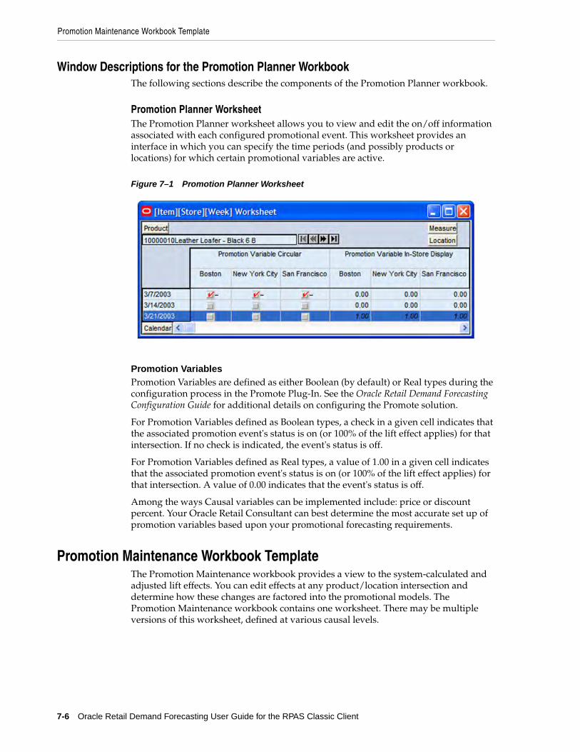
Promotion Maintenance Workbook Template
7-6 Oracle Retail Demand Forecasting User Guide for the RPAS Classic Client
Window Descriptions for the Promotion Planner WorkbookThe following sections describe the components of the Promotion Planner workbook.
Promotion Planner WorksheetThe Promotion Planner worksheet allows you to view and edit the on/off information associated with each configured promotional event. This worksheet provides an interface in which you can specify the time periods (and possibly products or locations) for which certain promotional variables are active.
Figure 7–1 Promotion Planner Worksheet
Promotion VariablesPromotion Variables are defined as either Boolean (by default) or Real types during the configuration process in the Promote Plug-In. See the Oracle Retail Demand Forecasting Configuration Guide for additional details on configuring the Promote solution.
For Promotion Variables defined as Boolean types, a check in a given cell indicates that the associated promotion event's status is on (or 100% of the lift effect applies) for that intersection. If no check is indicated, the event's status is off.
For Promotion Variables defined as Real types, a value of 1.00 in a given cell indicates that the associated promotion event's status is on (or 100% of the lift effect applies) for that intersection. A value of 0.00 indicates that the event's status is off.
Among the ways Causal variables can be implemented include: price or discount percent. Your Oracle Retail Consultant can best determine the most accurate set up of promotion variables based upon your promotional forecasting requirements.
Promotion Maintenance Workbook TemplateThe Promotion Maintenance workbook provides a view to the system-calculated and adjusted lift effects. You can edit effects at any product/location intersection and determine how these changes are factored into the promotional models. The Promotion Maintenance workbook contains one worksheet. There may be multiple versions of this worksheet, defined at various causal levels.

Promotion Maintenance Workbook Template
Promote (Promotional Forecasting) 7-7
Opening the Promotion Maintenance Workbook TemplateThe Promotion Maintenance wizard steps you through the process of creating a new Promotion Maintenance workbook from a template.
1. Within the Local or Simple domain, select New from the File menu.
2. On the Promote tab, select Promotion Maintenance. Click OK.
3. Select the promotion events to analyze. Click Next.
4. Select the causal forecast level for analysis. Click Next.
5. Select the locations to analyze. Click Next.
6. Select the products to analyze. Click Next.
7. Select additional measures to view in the workbook (if necessary). Click Finish.
Window Descriptions for the Promotion Maintenance WorkbookThe following sections describe the components of the Promotion Maintenance workbook.
Final PromoEffects WorksheetThe Final PromoEffects worksheet allows you to view and modify the system-calculated effects of a given promotion.
Figure 7–2 Final PromoEffects Worksheet
Measures: Final PromoEffects WorksheetThe Final PromoEffects worksheet contains the following measures:
System Calculated EffectThe System Calculated Effect is a read-only measure indicating the lift effect generated by the system.
System Effect OverrideThe user-specified lift effect. This user-entered effect is active if used in conjunction with the Override All and Override Future Only Promotion Effect Types. Otherwise, it equals 1.00.

Promotion Maintenance Workbook Template
7-8 Oracle Retail Demand Forecasting User Guide for the RPAS Classic Client
Promo Effect TypeCausal variable types define how causal variables are treated in the causal model fitting process (which includes a call to the lower level regression engine) and the forecast generation process where the model is used to extend the forecast over the forecast horizon. Table 7–1 lists the options.
Table 7–1 Causal Variable Types
Causal Variable Type Description
Automatic The inclusion of the causal variable is decided by regression. If the causal variable is found to be significant on the training set, it is included in the model. Otherwise, it is rejected. Automatic is the system default Promotion Effect Type.
Forced In The causal variable is forced in to the model, thus regression is not given a choice to reject even if the effect is considered insignificant by regression. As a result, we will always return an effect even if it has a negative impact to the demand forecast.
Disabled The variable is excluded from the model, hence no effect is returned either.
Override All This type allows you to specify a causal effect that is used during the fitting and forecasting process. This is a directive that is recognized only by the causal engine and not by the lower level regression engine. For causal variables specified as Override All, you also specify the corresponding causal effect in the Promotion Effect Override. The causal engine then de-causalizes the training data using the user-specified effect. The variable is then internally set to Disabled to calculate the fit. During forecast generation, the user-specified effect is used to determine the causal forecast. Therefore, you must change the Promotion Effect Type when this user-specified effect is no longer to be used.
Override Future Only This type allows you to specify a causal effect that is used only during forecasting process and not during the fitting process. This is also a directive that is recognized only by the causal engine and not by the lower level regression engine. For causal variables specified as Override Future, you also specify the corresponding causal effect in the Promotion Effect Override. The causal engine then internally sets the causal variable to Automatic to calculate the fit. The calculated effect is not written back to the effects array (so as to not overwrite the user specified effect). During forecast generation the calculated effect is ignored, and instead, the user-specified effect is used to produce a causal forecast. Therefore, you must change the Promotion Effect Type when this user-specified effect is no longer to be used.
Override from Higher Level
Used in conjunction with the Causal Higher Intersection set in the Forecast Administration Workbook, this promotion type allows the system to use the geometric mean of causal effects computed from product/location combination in the same group (the intersection level specified in the Causal Higher Intersection during system setup) for product/location combinations for which from sales history alone a causal effect is unable to be computed for that causal variable. The way the system handles this is by having the effects array filled in with higher-level effects for those variable specified as Override Higher Level and which did not have an effect returned in the previous run. The effect array is passed to the causal engine. If the engine succeeds in computing a significant effect, it writes back the system computed effect and uses it for generating a forecast. Otherwise, it uses the effect passed in (which as mentioned is the average effect among product stores belonging to the same group) for generating the forecast. Note that if no significant effects are found for any of the product/locations in the Causal Higher intersection group, then the system uses the geometric mean of causal effects calculated from all Product/Locations as the override effect being passed in.
Automatic Boolean If the promotion variable is always be set to 0.00 or 1.00 (meaning inactive or active, respectively), this type produces the same results as the Automatic type; however, Automatic Boolean improves the performance (speed) of the forecasting engine during the batch run of the forecast.

Promotion Effectiveness Workbook Template
Promote (Promotional Forecasting) 7-9
Promotion Effectiveness Workbook TemplateThe Promotion Effectiveness workbook template is a historical and future view to the effects of a planned promotion.
This workbook has two worksheets:
■ View of promotion effects
■ Visibility to Actuals, forecasts, baselines, and promotion variable/event information
In this workbook, you view the promotional forecast. There is also the ability to analyze the effects on the forecast if a promotion does or does not occur. This analysis is performed by turning a promotional event or attribute on or off for dates in the future plans, and/or by modifying the Simulated Effect. This workbook is intended for simulation and analysis purposes only. There is no Commit functionality.
Opening the Promotion Effectiveness Workbook TemplateThe Promotion Effectiveness wizard steps you through the process of creating a new Promotion Effectiveness workbook from a template.
1. Within the Local or Simple domain, select New from the File menu.
2. On the Promote tab, select Promotion Effectiveness. Click OK.
3. Select the causal level. Click Next.
4. Select the forecast level for analysis. Click Next.
5. Select the dates to analyze. Click Next.
6. Select the locations to analyze. Click Next.
7. Select the products to analyze. Click Next.
8. Select any additional measures that need to be included in the workbook (if necessary). Click Finish.
Note: Changes that are committed in the Promotion Maintenance workbook are not incorporated into the forecast until another forecast is generated in RDF batch forecast process.
Note: Changes to the Promotion Effectiveness workbook cannot be committed back to the master database; however, this workbook is useful for reporting on the performance of past promotions and simulating the effects of future promotions to support more accurate promotional modeling.

Promotion Effectiveness Workbook Template
7-10 Oracle Retail Demand Forecasting User Guide for the RPAS Classic Client
Window Descriptions for the Promotion Effectiveness WorkbookThe following sections describe the components of the Promotion Effectiveness workbook.
Promotion Variable/Effects WorksheetsThe Promotion Variable/Effects worksheets allow you to simulate the activation and de-activation of promotions, and it allows for promotion lift effects to be adjusted. The Promotion Variable/Effects worksheets are built at the hierarchy intersections of the promotion variables configured in the system, and at the product and location intersection of the causal forecast level selected during the wizard process. For example, if all of the variables are defined at the item/store/week level, only one worksheet would be built. However, if variables have been defined at different intersections, multiple worksheets is created based on each of the unique intersections. As well, if the causal forecast level selected for the workbook is the item/store/week level, an additional Promotion Variable/Effects worksheet is created at the item/store level in order to display the lift effect measures.
Figure 7–3 Promotion Variable/Effects [STR_ITEMWEEK] Worksheet
Figure 7–4 Promotion Variable/Effects [STR_ITEM] Worksheet

Promotion Effectiveness Workbook Template
Promote (Promotional Forecasting) 7-11
Measures: Promotion Variable/Effects WorksheetsThe Promotion Variable/Effects worksheets contain the following measures:
Promotion VariablesPromotion Variables are defined as either Boolean (by default) or Real types during the configuration process in the Promote Plug-In. See the Oracle Retail Demand Forecasting Configuration Guide for additional details on configuring the Promote solution.
For Promotion Variables defined as Boolean types, a check in a given cell indicates that the associated promotion event's status is on (or 100% of the lift effect applies) for that intersection. If no check is indicated, the event's status is off.
For Promotion Variables defined as Real types, a value of 1.00 in a given cell indicates that the associated promotion event's status is on (or 100% of the lift effect applies) for that intersection. A value of 0.00 indicates that the event's status is off.
Among the ways causal variables can be implemented includes: price, percent contribution of the lift effect, or discount percent. Your Oracle Retail Consultant can best determine the most accurate set up of promotion variables based upon your promotional forecasting requirements.
Approved EffectThis is a read-only measure. This is the approved promotion lift effect used in the generation of the current System Forecast in RDF.
Simulated EffectThis is a read/write measure. The Simulated Effect defaults to the Approved Effect. Changes to this measure has an impact to the Historical Forecast and the Future Forecast.
System Calculated EffectThe System Calculated Effect is a read-only measure. This is the promotion lift effect originally calculated by the system during the forecast generation process. This value can be different from the Approved Effect if you edited the System Effect Override in the Promotion Maintenance workbook, and then another batch forecast was run.
Promotion Analysis WorksheetThe Promotion Analysis worksheet is created at the same base intersection as the causal forecast level selected during the wizard process. Changes made to the Promotion Variables and Simulated Promo Effect on the Promotion Effectiveness worksheet is reflected in the recalculation of the Historical Forecast and Future Forecast.
Note: The Approved Effect, Simulated Effect, and System Calculated Effect are only visible on the worksheet that is at the same product and location intersection as the causal forecast level selected during the wizard process.

Promotion Effectiveness Workbook Template
7-12 Oracle Retail Demand Forecasting User Guide for the RPAS Classic Client
Figure 7–5 Promotion Analysis Worksheet
Measures: Promotion Analysis WorksheetThe Promotion Analysis worksheet contains the following measures:
History Data (the measure that represents Sales/Actuals)This is a read-only measure. History Data is the sales data used to generate the forecast. This allows you to compare Actuals to forecast values. When the workbook is created, the Data Source specified in the Forecast Administration Workbook is included in the Promotion Analysis.
System ForecastThis is a read-only measure. This is the latest forecast quantity approved for the product/location combination.
Promotional PeakThis is a read-only measure. The Promotional Peak is the unit-lift over the Baseline Forecast calculated during the forecast generation process.
Future BaselineThis is a read-only measure. Calculated as the System Forecast minus (-) the Promotional Peaks. User-changes to the editable measures in the Promotion Variable/Effects worksheets do not affect this value.
Future ForecastThis is a read-only measure. The Future Forecast equals the Future Baseline multiplied by the Simulated Effect if the promotion variable is greater than 0 (zero). If there are more than one promotion variables, the sum of the Simulated Effects for the variables is multiplied by the Future Baseline.
If there is no active promotion variable, the Future Forecast equals the Future Baseline.
Note: Changes that are committed in the Promotion Maintenance workbook are used to determine values for the System Calculated Effect and the Approved Effect. However, if a forecast has not been generated in RDF since the changes were made in the Promotion Maintenance workbook, the System Forecast does not include these changes.

Promotion Management Workbook Template
Promote (Promotional Forecasting) 7-13
Historical BaselineThis is a read-only measure. Calculated in one of two ways based on the value of the System Forecast:
■ Historical Baseline equals Sales minus the Promotion Peak if the System Forecast is greater than 0 (zero).
■ Historical Baseline equals Sales with the Moving Average applied if the System Forecast equals 0 (zero). If Sales are also 0 (zero), the Historical Baseline also equals 0 (zero).
Historical ForecastThis is a read-only measure. The Historical Forecast equals the Historical Baseline multiplied by the Simulated Effect if the promotion variable is greater than 0 (zero). If there are more than one promotion variables, the sum of the Simulated Effects for the variables is multiplied by the Historical Baseline.
If there is no active promotion variable, the Historical Forecast equals the Historical Baseline.
Promotion Management Workbook TemplateThe Promotion Management workbook template allows you to enable and disable promotions for causal forecast levels and to specify whether promotions can have a negative effect.
This workbook has these worksheets:
■ Promotion Enable Worksheet
■ Accept Negative Lift Worksheet
Opening the Promotion Management Workbook TemplateThe Promotion Management wizard helps you create a new Promotion Management workbook from a template.
1. Within the Local or Simple domain, select New from the File menu.
2. On the Promote tab, select Promotion Management.
Click OK.
3. Select the causal level.
Click Next.
4. Select the promotions.
Click Finish.
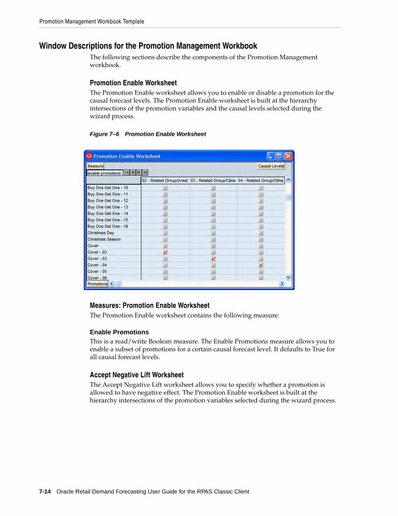
Promotion Management Workbook Template
7-14 Oracle Retail Demand Forecasting User Guide for the RPAS Classic Client
Window Descriptions for the Promotion Management WorkbookThe following sections describe the components of the Promotion Management workbook.
Promotion Enable WorksheetThe Promotion Enable worksheet allows you to enable or disable a promotion for the causal forecast levels. The Promotion Enable worksheet is built at the hierarchy intersections of the promotion variables and the causal levels selected during the wizard process.
Figure 7–6 Promotion Enable Worksheet
Measures: Promotion Enable WorksheetThe Promotion Enable worksheet contains the following measure:
Enable PromotionsThis is a read/write Boolean measure. The Enable Promotions measure allows you to enable a subset of promotions for a certain causal forecast level. It defaults to True for all causal forecast levels.
Accept Negative Lift WorksheetThe Accept Negative Lift worksheet allows you to specify whether a promotion is allowed to have negative effect. The Promotion Enable worksheet is built at the hierarchy intersections of the promotion variables selected during the wizard process.

Promotion Management Workbook Template
Promote (Promotional Forecasting) 7-15
Figure 7–7 Accept Negative Lift Worksheet
Measures: Accept Negative Lift WorksheetThe Accept Negative Lift worksheet contains the following measure:
Promotion Allow Negative LiftThis is a read/write Boolean measure. The Promotion Allow Negative Lift measure allows you to specify whether a promotion is allowed to have negative effect. When this measure is set to False for a promotion, the forecast engine does not allow that promotion to have any negative lift (Effect < 1). It defaults to True for all promotions.
Procedures in Promotional ForecastingThe following list outlines the standard procedures performed in order to set up the system to run a promotional forecast (more detailed steps follow in the next section):
■ Set up the system to run a promotional forecast
■ Set forecast parameters in the Forecast Administration Workbook
■ Set forecast parameters in the Forecast Maintenance Workbook
■ Set promotions to be active in the Promotion Planner Workbook Template
■ Run the batch forecast
■ View and Edit Causal Forecast results
■ Analyze forecasts in the Forecast Approval Workbook
■ Analyze and edit causal effects in the Promotion Maintenance Workbook Template
■ Promotion Simulation (What-if) and Analysis

Promotion Management Workbook Template
7-16 Oracle Retail Demand Forecasting User Guide for the RPAS Classic Client
Setting Up the System to Run a Promotional ForecastPerform the following procedure to set up the system to run a promotional forecast.
1. On the Forecast tab, select and build a Forecast Administration Workbook.
1. In the Forecast Administration Workbook: Advance Parameter worksheet, select Generate Baseline.
2. Optional: Set the Default Forecast Method to Causal for the desired level if the level is to be use only for Promotional Forecasting.
3. Optional: Set the Causal Higher Intersection for the desired level if the Override from Higher Level promotion type is used.
4. Optional for use with Daily Causal Forecasting: Set the values for the following parameters:
– Causal Aggregation Profile
– Causal Calculation Intersection
– Causal Calculation Intersection Periodicity
5. Commit your changes to the master database by selecting Commit Now from the File menu.
2. On the Forecast tab, select and build a Forecast Maintenance workbook.
1. Set the Forecast Method Override to Causal for any items/locations at the desired levels that use Promotional Forecasting.
2. Commit your changes to the master database by selecting Commit Now from the File menu.
3. On the Forecast tab, select and build a Promotion Planner workbook.
1. Set causal variables for items and locations historically in that the selected promotions are active.
2. Commit your changes to the master database by selecting Commit Now from the File menu.
4. On the Forecast tab, select Run Batch.
■ Generate a Forecast.
Viewing a Forecast That Includes Promotion EffectsPerform this procedure to view a forecast that includes promotion effects.
1. On the Forecast tab, select and build a Forecast Approval Workbook and include System Baseline in your workbook.
2. In the Final Level worksheet, review the System Baseline and the System Forecast. The System Baseline is predicted demand given no causal effects. The System Forecast is the sum of the System Baseline and the Promotional Peak calculated during the forecast generation process based on the causal data and settings.

Promotion Management Workbook Template
Promote (Promotional Forecasting) 7-17
Viewing and Editing Promotion System-Calculated EffectsPerform this procedure to view and edit promotion system-calculated effects.
1. On the Promote tab, select and build a Promotion Maintenance workbook.
1. In the PromoEffects worksheet, review the System-Calculated Effect.
2. If the System Calculated Effect is to be modeled using a method other than Automatic, edit the Promotion Effect Type.
3. If you choose to adjust the system-calculated effect, adjustments can be made to the System Effect Override. You must also set the Promotion Effect Type to Override All or Override Future Only.
2. On the Forecast tab, select Run Batch.
■ Generate a Forecast.
Promotion Simulation (What-if?) and AnalysisFollow this procedure to perform analysis on past promotions and simulate the effects of historic or future promotions:
1. On the Promote tab, select and build a Promotion Effectiveness workbook.
2. In the Promotion Variable/Effects worksheet review the Promotion System-Calculated Effect and edit the Simulated Promo Effect, then select Calculate to recalculate the Future Forecast.
Note: Changes to the Promotion Effects workbook cannot be committed; however, this workbook is useful for:
■ Reporting on the performance of past promotions.
■ Simulating the effects of future promotions to support more accurate promotional modeling.

Promotion Management Workbook Template
7-18 Oracle Retail Demand Forecasting User Guide for the RPAS Classic Client

8
Curve 8-1
8Curve
Curve is an optional automated predictive solution that can generate ratio arrays from historical data at user-specified intersections. The profiles generated by Curve can be used for various purposes; for example, to convert the organization-level assortment plans into base-level weekly sales forecasts and to generate seasonal forecasts, daily forecasts, or new product forecasts using lifecycle profiles.
Curve meets the need of operational systems (such as Oracle Retail Demand Forecasting [RDF] and Oracle Retail Merchandising System [RMS]) to have sales unit predictions at a more detailed level than those provided by planning programs. The planning process attempts to establish the correct balance between different products in order to maximize sales opportunities in the available sales space. The planning process is supported by the generation of an assortment plan, which provides details of your anticipated sales volumes and stock requirements at aggregated levels. However, operational systems like RDF requires data to be at the lowest level of execution (that is, item/store/week or item/store/day) because these systems are responsible for ensuring that the right quantity of each product is in the right store at the right time.
In the most basic sense, a profile represents the ratio of an aggregate dimension to the dimension for execution. For example, you may have a forecast generated at the item/store/week level, but for execution purposes the data must be spread down to the item/store/day level. It is the point of aggregation (source level) and the desired destination intersection (final profile) that are the unique identifiers of each profile. Using this example, the point of aggregation of the data (where the data equals 100%) is item/store/week, and the desired destination intersection (where all data ratios sum to 100%) is item/store/day.
There are several parameters within RDF that may take a Curve-generated profile as an input. These are: Causal Aggregation Profile, Causal Spread Profile, Seasonal Profile and Spreading Profile. The most common input from Curve that is required by RDF is the Spreading Profile. This profile can either be manually generated and approved by the user or dynamically generated as part of the RDF batch forecast process. For more information on the different profile parameters in RDF, refer to the Oracle Retail Demand Forecasting User Guide.

Dynamic Profiles
8-2 Oracle Retail Demand Forecasting User Guide for the RPAS Classic Client
Dynamic ProfilesDynamic Profiles are generated as part of the RDF forecast batch process to produce ratios used to spread source level forecasts to a final forecast level. To specify a profile to be generated in such a manner, the profile name (the level number of the profile, 01 for example) is entered in Spreading Profile field in RDF. When the batch forecast is executed, RDF produces an interim forecast at the final forecast level.
This interim forecast becomes the Profile Data Source in Curve and is used to generate the final profile. The final profile is then passed back to RDF to determine the final forecast results. For information on profile configuration for integration with RDF see both the Oracle Retail Curve Configuration Guide and Oracle Retail Demand Forecasting Configuration Guide.
Profile Maintenance WorkbookAfter setting default parameters for profile generation in the Profile Administration Workbook, the next step in profile generation is to select any subset of positions for which the values set in Profile Administration differ from the defaults. This step is necessary in those situations where it is not efficient to use the same parameters for all positions in the hierarchy data.
The Profile Maintenance Workbook allows edits to intersections that vary from the default values set in the Profile Administration Workbook.
Creating a Profile Maintenance WorkbookAs in Profile Administration, the first Profile Maintenance wizard screen prompts you to select a final profile level.
1. Within the Master, Local, or Simple domain; select New from the File menu.
2. Select the Curve tab to display a list of workbook templates for Profiling.
3. Select Profile Maintenance. Click OK.
4. The Profile Maintenance Wizard opens and prompts you to select the final profile. Make the appropriate selection, and click Next.
5. If the Location hierarchy is defined in the profile, select the locations to include in the workbook, and click Next.
6. If the Merchandise hierarchy is defined in the profile, select the products to include in the workbook, and click Next.
7. If the Calendar hierarchy is defined in the profile, select the time periods to include in the workbook, and click Next.
8. An additional wizard screen will prompt you to select any additional measures (that is, measures not standard in the Profile Maintenance Workbook) that you would like included. The measure options available in this screen are set in the RPAS Security Administration Workbook / Workbook Template Measure Rights Worksheet. Make the appropriate selections (if any). Click Finish to display the workbook.

Profile Maintenance Workbook
Curve 8-3
Final Approval and Sourcing Worksheet
Figure 8–1 Final Approval and Sourcing Worksheet
Measures: Final Approval and Sourcing WorksheetThe following is a description of the measures contained in the Final Approval and Sourcing Worksheet:
Profile Approval MethodThe Profile Approval Method displays the primary approval policy that is used for the profile. No Override is displayed in this field if the Default Approval Method is used. Select Approve Use System if profile results are to be automatically approved during the batch profile generation. Select Do Not Approve if profile results are to be manually approved by the user. If a profile is being generated dynamically (to support Source Level Forecasting) as part of the RDF batch forecast process, the Default Profile Approval Method should be set to Approve Use System.
Source Profile OverrideMake edits to the Source Profile Override if the source level for an intersection varies from the Default Source Profile. No Override is displayed in this field if the value set in the Default Source Profile is to be used. When only a single source is configured for a profile, all profile results are calculated using the same intersections. Therefore, edits to this parameter are not required. When multiple sources are defined for a profile, some profile results are calculated using different intersections. Select the appropriate source level for an intersection.

Profile Administration Workbook
8-4 Oracle Retail Demand Forecasting User Guide for the RPAS Classic Client
Final Training Window Worksheet
Figure 8–2 Final Training Window Worksheet
Measures: Final Training Window WorksheetThe following is a description of the measures contained in the Final Approval and Sourcing Worksheet:
System Training Window BeginSelect a date in this field if this date is different from the default value set in the Training Window Start date in Profile Administration. Click the pop-up calendar to change the value in this field.
System Training Window EndSelect a date in this field if this date is different from the default value set in the Training Window End date in Profile Administration. Click the pop-up calendar to change the value in this field.
Profile Administration WorkbookThe Profile Administration Workbook allows you to set default parameters for profile generation, which is the first step in profile generation. These parameters are typically set during system implementation, and are configured based on your business practices and needs. This configuration can be updated if you need to change certain parameters over time. However, it is not practical to change the configuration on a regular basis. The Profile Administration Workbook gives you the flexibility to change profiling parameters as the need arises to improve both forecasting accuracy and computational efficiency.
Selecting a Final Profile to EditThe Profile Administration wizard requires you to select the final profile that you want to edit. These profiles are determined during the system implementation/configuration.
1. Within the Master, Local or Simple domain, select New from the File menu.
2. On the Curve tab, select Profile Administration. Click OK.
3. Select the final profile to analyze. Click Finish.

Profile Administration Workbook
Curve 8-5
Profile Parameter WorksheetThe Profile Parameter Worksheet allows you to specify default values for parameters effecting profile generation. The following image provides an example of the Profile Parameters worksheet in a Master Domain with three partitions/Local Domains, partitioned on Group.
Figure 8–3 Profile Parameter Worksheet
Measures: Profile Parameter WorksheetThe following is a description of the measures that are contained in the Profile Parameter Worksheet:
Default Phase EndThe Default Phase End defines the end date of the period in which profile results will be applied. Click the pop-up calendar to change the value in this field. If phase definitions are unavailable, the default phase end date will be used. When calculating time profiles, default dates are used for intermediate computations. For computational efficiency, use the most common phase definition as the default value.
Default Phase StartThe Default Phase Start defines the first date of the period in which profile results will be applied. Click the pop-up calendar to change the value in this field. If phase definitions are unavailable, the default phase start date will be used. When calculating time profiles, default dates are used for intermediate computations. For computational efficiency, use the most common phase definition as the default value.

Profile Administration Workbook
8-6 Oracle Retail Demand Forecasting User Guide for the RPAS Classic Client
Default Profile Approval MethodThe Default Profile Approval Method displays the primary approval policy to be used for the profile. Select Approve Use System if profile results are to be automatically approved during the batch profile generation. Select Do Not Approve if profile results are to be manually approved by the user. If a profile is being generated dynamically (to support Source Level Forecasting) as part of the RDF batch forecast process, the Default Profile Approval Method should be set to Approve Use System.
Default Source ProfileThe Default Source Profile determines the primary source level that will be used to generate the profile. When only a single source is configured for a profile, all profile results will be calculated using the same intersections. When multiple sources are defined for a profile, some profile results will be calculated using different intersections. The Profile Maintenance Workbook may be used to define exceptions to the Default Source Profile.
Default Training Window End The Default Training Window End defines the last date in history that will be used to calculate profile results. Click the pop-up calendar to change the value in this field. The default date will be used only if the training window method is set to Defaults and Overrides.
Default Training Window Start The Default Training Window Start defines the first date in history that will be used to calculate profile results. Click the pop-up calendar to change the value in this field. The default date will only be used if the training window method is set to Defaults and Overrides.
Normal ValueIf the profile is aggregated to the Aggregation Intersection, this will be the value in all the cells (or zero outside of the phase window). The desired setting for Normal Value is usually 1.00 (100%); however, there may be instances where it is desired to have the profile normalize to a value different than 1.00. For example, when generating seasonal profiles, such as by Week of Year, the Normal Value needs to be set to 52.
Profile Data SourceThe Profile Data Source displays the name of the measure that contains the data to be used to generate the profile.
Profile TypeThe Profile Type is a read-only measure that displays the value for this measure set in the Curve Plug-In. The Profile Type is used to determine the profile algorithm and validation required by the profile level. Profile Types are represented with pre-defined configuration information.
Note: For Dynamic profiles used by RDF, the profile Data Source can be left blank. Curve will use the Interim Forecast generated by RDF as the Data Source for generating the profile, and the value specified here will be ignored.

Profile Administration Workbook
Curve 8-7
The following Profile Types share the same profile algorithm. The rationale for providing different types that have the same behavior is strictly to remind the user of the intent of the profile while using this workbook:
■ Store Contribution Profile - The Store Contribution Profile is used to determine the data relationship between stores to aggregate dimensions in the location hierarchy.
■ Daily Profile - The Daily Profile is used to determine the data relationship between a given day to the week in which it belongs.
■ Hourly Profile - The Hourly Profile is used to determine the spreading ratios from aggregate dimensions to the hour, hour of day, or hour of week dimensions.
■ Product Profile - The Product Profile is used to determine the data relationship between any two dimensions along the product hierarchy.
■ Size Profile - Size profiles are used to determine the data relationship between any size in the product hierarchy and another dimension in the product hierarchy. Note that size can be configured as a dimension along an alternate rollup along the product hierarchy, such as itemParent-size.
■ User Defined Profile - The User Defined Profile may be used to support any basic profile configuration.
The following Profile Types have unique behavior:
■ Diff Profile - Diff Profiles are used to determine spreading ratios from aggregate dimensions in the Product hierarchy to diff dimensions. Used to support the spreading of data in RMS Allocation, Diff Profiles exhibit the same behavior as the previous profile types. However, unique to Diff Profiles is special validation of the relationship between the defined diff dimensions to dimensions along the main branch of the Product hierarchy. See the RDF Administration Guide for more information on validation criteria.
■ Daily Seasonal Profile - The Daily Seasonal Profile is used to determine the data relationship between a given day of the week to aggregate dimensions in the calendar hierarchy. This profile type uses training window data to compute the profile. The resulting profile is then clipped to fit within the defined phase window.
■ Life Cycle Profile - The Life Cycle Profile uses data along a user-defined training window, and then stretches or shrinks data to fit a user-defined phase window.
RenormalizeRenormalize is a Boolean measure. When set to TRUE, it will automatically renormalize the calculated profile result at the corresponding final level. Normally, the renormalization is not necessary. For example, if you have a source profile at week of season and its final profile is at day of season, you would need to renormalize the final level because going from week to day will do replication. At day level, the profile will sum up to greater than 1 for a season. Since it was a week to day, it will probably sum up to seven. The renormalize will force the final profile to sum to 1.00 (100%).
System Training Window LengthThe System Training Window Length is necessary when Use Training Window is set as the Training Window Method for the profile. This field specifies the number of weeks of the most recent data to use as the training window for calculating the profile. The System Training Window Length defaults to 10 weeks.

Profile Administration Workbook
8-8 Oracle Retail Demand Forecasting User Guide for the RPAS Classic Client
Training Window MethodThe Training Window Method is used to determine the default method that is used to define the training window. The options are:
■ Default and Overrides - Uses the default dates as set in the Training Window Start Date and Training Window End Date measures.
■ Phase Definitions and Overrides - Calculates the Training Window Start Date and Training Window End Date based on the Phase Start Date and Phase End Date measures.
■ Use Training Window - Used with System Training Window Length to specify the number of weeks of the most recent data to use for calculating the profile.
Use Advanced Profile FeaturesThis parameter is set to true (checked) by default; however, if dynamic profiles are being generated during the RDF batch process, setting this parameter to false (unchecked) improves batch performance by skipping unnecessary processes in the creation of the dynamic profiles.
When this is set to false, RDF will automatically roll the Training window and Phase windows forward with the forecasts for Dynamic profiles. If this is set to true, the user will have to manually manage any forecast date adjustments for these windows.
Profile and Source Level Intersection WorksheetThe Profile and Source Level Intersection Worksheet is a read-only view to the different intersections defined for the Profile and Source level configured in the Curve Plug-in. See the RPAS Solution Extension Configuration Guide for more information on defining these intersections during configuration of the Curve Solution.
Figure 8–4 Profile and Source Level Intersection Worksheet
Measures: Profile and Source Level Intersection Worksheet
Profile Agg IntersectionThe Profile Agg Intersection is the intersection where the profile will sum to one (or 100%). If the profile is being used as the Spreading Profile in RDF, this Aggregation Intersection should be the same as the Source Forecast Level.

Profile Approval Workbook
Curve 8-9
Profile Approval IntersectionAssigned only at the Final Profile, the Approval Intersection is the intersection where the profile is approved. Approval Intersection should be above or equal to the Aggregation Intersection. If the profile is being used as the Spreading Profile in RDF, this Approval Intersection should be the same as the Aggregation Intersection.
Profile IntersectionThe Profile Intersection is the intersection where an intermediate profile is calculated. This intermediate profile is then replicated down or aggregated up to the Stored Intersection. If the Store Intersection is the same as the Profile Intersection, the values in intermediate profile are copied to the Stored Intersection. The Profile Intersection must be lower than the Aggregation Intersection. If the profile is being used as the Spreading Profile in RDF, this Profile Intersection should be the same as the Final Forecast Level.
Stored IntersectionThe Stored Intersection is the destination intersection of the profile. The intermediate profile produce at the Profile Intersection is either replicated down to or aggregated up to the Stored Intersection. If the Store Intersection is the same as the Profile Intersection, the values in intermediate profile are copied to the Stored Intersection. The Stored Intersection not should be greater than the Aggregation Intersection. If the profile is being used as the Spreading Profile in RDF, this Stored Intersection should be the same as the Profile Intersection.
Profile Approval WorkbookThe profiles generated at the historic levels must be viewed, analyzed, revised, and approved using the Profile Approval Workbook. In the approval process, you select the appropriate source level for each product/location combination. After you make any necessary changes to the profiles and commit the workbook, the profiles are normalized to preserve the appropriate ratios. At this time, Curve automatically spreads the source level profiles to the final level and combines them. After you commit your changes, you can refresh the data in your workbook to display the newly generated final level profiles.
Use the Profile Approval Workbook to view, analyze, revise, and approve the profiles generated at the historic levels. This workbook contains three tabs for each worksheet displayed:
■ Final Worksheet
■ Source Worksheet
■ Approval Worksheet
Creating a New Profile Approval Workbook1. With the Local or Simple domain, select New from the File menu.
2. Select the Curve tab to display a list of workbook templates.
3. Select Profile Approval. Click OK.
4. The Profile Approval Wizard opens and prompts you to select the final profile. Make the appropriate selection. Click Next.
5. If the Location hierarchy is defined in the profile, select the locations to include in the workbook. Click Next.

Profile Approval Workbook
8-10 Oracle Retail Demand Forecasting User Guide for the RPAS Classic Client
6. If the Merchandise hierarchy is defined in the profile, select the products to include in the workbook. Click Next.
7. If the Calendar hierarchy is defined in the profile, select the time periods to include in the workbook. Click Next.
8. An additional wizard screen will prompt you to select any additional measures (that is, measures not standard in the Profile Approval Workbook) that you want to include. The measure options available in this screen are set in the RPAS Security Administration Workbook / Workbook Template Measure Rights Worksheet. Make the appropriate selections (if any). Click Finish to display the workbook.
Final Profile WorksheetThrough this worksheet, you can view the system calculated final profile and make adjustments to this profile. Following is an example Final Profile Worksheet for a day of week profile.
Figure 8–5 Final Profile Worksheet
Measures: Final Profile Worksheet
Adjusted ProfileThis is the user-adjusted profile. If edits are necessary to the Adjusted Profile, it is first required to lock the Adjust Profile at the Aggregation Intersection. This will prevent the Normal Value from recalculating to a value different than 1.00 (100%) when the adjustments are made. To determine the Aggregation Intersection, view the intersection displayed on the Approval worksheet. Once adjustments are made to the profile, the user must go to the Final Profile Approval Worksheet and set the 'Do Not Approve' flag to true for the adjusted intersection. The Approved Profile measure will update with these changes.
Approved ProfileThe Approve Profile displays the approved profile values. If a profile intersection is set to Do Not Approve, no value will be displayed in this field. The system will automatically approve all profile intersections set to Approve Use System. If changes
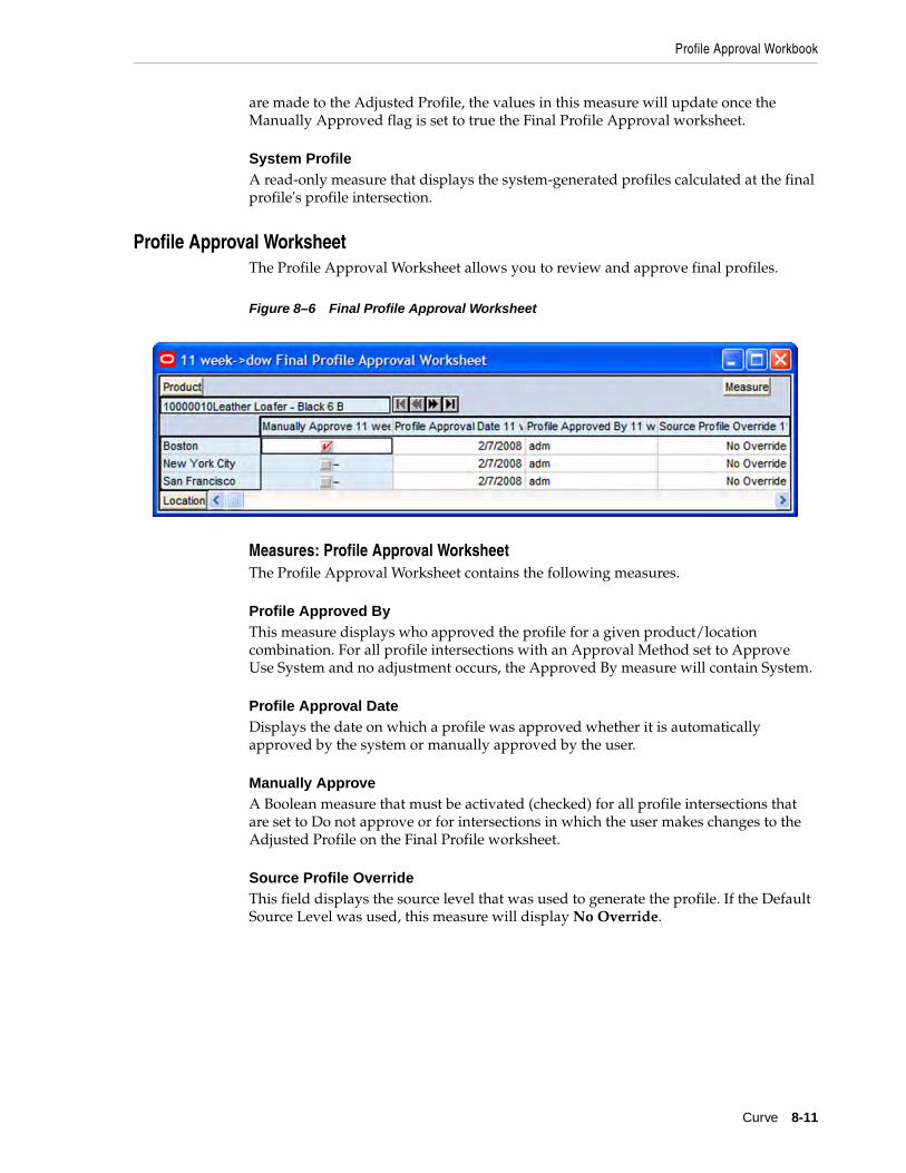
Profile Approval Workbook
Curve 8-11
are made to the Adjusted Profile, the values in this measure will update once the Manually Approved flag is set to true the Final Profile Approval worksheet.
System ProfileA read-only measure that displays the system-generated profiles calculated at the final profile's profile intersection.
Profile Approval WorksheetThe Profile Approval Worksheet allows you to review and approve final profiles.
Figure 8–6 Final Profile Approval Worksheet
Measures: Profile Approval WorksheetThe Profile Approval Worksheet contains the following measures.
Profile Approved ByThis measure displays who approved the profile for a given product/location combination. For all profile intersections with an Approval Method set to Approve Use System and no adjustment occurs, the Approved By measure will contain System.
Profile Approval DateDisplays the date on which a profile was approved whether it is automatically approved by the system or manually approved by the user.
Manually ApproveA Boolean measure that must be activated (checked) for all profile intersections that are set to Do not approve or for intersections in which the user makes changes to the Adjusted Profile on the Final Profile worksheet.
Source Profile OverrideThis field displays the source level that was used to generate the profile. If the Default Source Level was used, this measure will display No Override.

Generate Profiles
8-12 Oracle Retail Demand Forecasting User Guide for the RPAS Classic Client
Source Profile WorksheetThe Source Profile Worksheet displays the profiles generated at the source level for all product/location/calendar combinations selected to appear in the workbook. This worksheet displays the source system profiles (that is, the profiles that are calculated by the system during the profile generation process).
Figure 8–7 Source Profile Worksheet
Measures: Source Profile WorksheetThe following measure is contained in the Source Level worksheet:
System ProfileA read-only measure that displays the system-generated profiles calculated at the source profile's profile intersection for each product/location combination displayed.
Generate ProfilesThe batch profile generation process creates profile results for all hierarchy positions set in the Profile Intersection. Profiles may be run from the backend of the domain using the curvebatch executable or run manually using the Run Batch Profile template. For more information on curvebatch, see the Oracle Retail Predictive Application Server Administrators Guide.
Generating a Profile Manually1. With the Local or Simple domain, select New from the File menu.
2. Select the Curve tab to display a list of workbook templates. Select Run Batch Profile and click OK.
3. The Run Batch Profile Wizard opens and prompts you to select the profiles to generate. Select Next or Finish.
The Run Batch Profile wizard automatically executes curvebatch within the Simple or Local Domain. If Next is selected from the last wizard screen, the wizard will not advance to the completion message until the profiles have been generated. Depending on the data set, this process may take a several minutes before the system advances to the final screen.

9
Grade 9-1
9Grade
Grade is a clustering tool that provides insight into how various parts of a retailer's operations can be grouped together. Typically, a retailer may cluster stores over item sales to create logical groupings of stores based upon sales of particular products. This provides increased visibility to where products are selling, and it allows the retailer to make more accurate decisions in merchandising. Beyond this traditional use of clusters, Grade is flexible enough to cluster any business measure based on products, locations, time, promotions, customers, or any hierarchy configured in the solution. Key Grade functionality includes:
■ Two methods of creating Grades/Clusters:
■ Breakpoints: the sorting of data points into groups based on user-defined indexes
■ Clustering, or the BaNG, Algorithm: the optimization of data points into clusters based on the user-defined number of clusters
■ Group By capabilities: support the segmentation of clusters for more detailed and focused cluster generation
■ Clustering statistics: provide insight into the relationship of members within a cluster and how all clusters relate to one another
■ Cluster What-if: allows user changes to members assigned to clusters and the review of recalculated clustering statistics
Regardless of the method employed to create clusters, Grade is designed to support the decision-making process necessary to create effective and actionable groupings of data. The following chapters describe the process to generate Grades/clusters and analyze results. All of Grade's functionality exists in the following templates:
■ Breakpoints Administration workbook
■ Generate Breakpoint Grades wizard
■ Generate Clusters wizard
■ Cluster Review workbook
■ Delete Clusters wizard
Information on the functionality of the above templates is provided in the following sections.

Cluster Methods in Grade
9-2 Oracle Retail Demand Forecasting User Guide for the RPAS Classic Client
Cluster Methods in GradeGrade supports two cluster methods: Breakpoint and Batch Neural Gas Algorithm (BaNG).
Index to AverageIndex to Average is the average sales of the stores in each grade divided by the average sales of all stores. This value provides a relative indication of how well a grade performed compared to the total store average. A value of 1.00 indicates that average sales in the grade were the same as average sales across the chain. A value of 3.74, for example, indicates that average sales in the grade were 3.74 times the chain average.
BreakpointBreakpoint method clusters, or groups, data points based on user-defined thresholds, or breakpoints. Breakpoints are properly defined by entering a decreasing sequence of real numbers that terminate in a value of zero. Breakpoints are entered in the breakpoints administration workbook. Breakpoints are then used to cluster data points based on the index to average of each data point.
Example 9–1 Breakpoint
While clustering stores, if the user has entered the breakpoints 2.0, 1.5, 1.0, 0.5, and 0.0, the system will generate five grades. Stores that sell more than 2.0 times the average sales (over all stores) will be assigned to the highest grade, and stores that sell less than 0.5 times the average will be assigned to the lowest grade.
Batch Neural Gas Algorithm (BaNG)The BaNG algorithm automatically generates optimal clusters based on user-specified number of clusters and clustering criteria. The algorithm provides a means for clustering data based on data distributions. For example, while clustering on weekly store sales data, the BaNG algorithm considers the Euclidean distance of the individual Store/week level data points from a cluster center to determine the clusters. This is different from the Breakpoint method, where clustering is performed based on average sales.
The BaNG algorithm iteratively updates cluster centers while considering the distance of each data vector from the cluster centers and its contribution to each cluster center. For every data point, cluster centers are ranked based on their distance from the data point within each iteration.
Additionally, the cluster centers are guided, using a control parameter, to gradually spread from the center of the distribution to their optimal locations.
The BaNG algorithm is a non-trivial extension of the K-means clustering approach. It is usually faster than the K-means, and is guaranteed to converge.
BaNG versus BreakpointThe BaNG algorithm generates statistically optimal clusters based on the number of clusters specified by the user. Breakpoint generates clusters based on user input breakpoints, and the number of clusters generated depends on the breakpoints.
In order to generate store clusters that vary by Department, users need to specify a group by option of Department Breakpoint will cluster stores based on average store sales within each Department, while BaNG can consider an additional dimension for

Breakpoints Administration Workbook
Grade 9-3
generating the clusters. For example, BaNG can cluster based on weekly sales of each stores within the Department Here, weekly sales are the coordinates over which the clustering is performed.
Grade in a Global Domain EnvironmentWhen implemented in a global domain environment, the following workbooks are available to be accessed from the Master domain:
■ Breakpoint Administration
The remaining Grade workbooks can only be accessed from local domains. These include:
■ Cluster Review
■ Delete Cluster Run
■ Generate Breakpoint Grades
■ Generate Clusters
Breakpoints Administration WorkbookThe Breakpoints Administration workbook is used with the breakpoints method of grading. In this workbook, the user sets the index to average for each breakpoint. This includes the ability to set multiple breakpoint configurations to allow for Grades to be produced and compared using different breakpoint settings.
Creating a Breakpoints Administration Template Workbook1. In the Simple or Local Domain, select New from the File menu.
2. Select the Grade tab to display a list of workbook templates.
3. Select Breakpoints Administration. Click OK.
Breakpoint Administration Worksheet If the breakpoints method is to be used to generate grades, you must go through the process of setting of the Index to Average for each grade's breakpoint range. The following is an example of the Breakpoint Administration worksheet:
Note: The Breakpoint Administration workbook is accessible from the Master domain to allow for the centralized administration of breakpoints.

Breakpoints Administration Workbook
9-4 Oracle Retail Demand Forecasting User Guide for the RPAS Classic Client
Figure 9–1 Breakpoint Administration Worksheet
On the Breakpoint Administration worksheet, for a Configuration/Cluster intersection, set the Index to Average to be used by the Breakpoints algorithm for sorting data points into grades. The number of configurations available in this worksheet is based on the Maximum Number of Clusters configured in the Grade Plug-In. Only one configuration is required for use with the breakpoints method.
Breakpoints should be set from high Index to Average to low Index to Average starting with the first Cluster ordered in the list of available clusters.
In Figure 9–1, the Index to Average is set as the following for Configuration 01:
■ 1 Cluster01: 1.25
■ 2 Cluster02: 0.75
■ 3 Cluster03: 0.50
■ 4 Cluster04: 0.25
■ 5 Cluster05: 0.00
Using this example, the Breakpoints algorithm groups data based on the following:
Note: The Cluster Labels may vary based on the configuration.
Data Description
1 Cluster01 Sort all data with an Index to Average at or above 1.25 into 1 Cluster01.
2 Cluster02 Sort all data with an Index to Average from 0.75 to 1.24 into 2 Cluster02.
3 Cluster03 Sort all data with an Index to Average from 0.50 to 0.74 into 3 Cluster03.
4 Cluster04 Sort all data with an Index to Average from 0.25 to 0.49 into 4 Cluster04.
5 Cluster05 Sort all data with an Index to Average from 0.00 to 0.24 into 5 Cluster05.

Generate Breakpoint Grades Using the Breakpoints Method
Grade 9-5
Generate Breakpoint Grades Using the Breakpoints MethodThe Generate Breakpoint Grades wizard allows you to range the input data and hierarchies that will be used to produce grades based on the Breakpoints method.
Opening the Generate Breakpoint Grades Template Wizard1. Within the Simple or Local Domain, select New from the File menu.
2. Select the Grade tab to display a list of workbook templates.
3. Select Generate Breakpoints Grades. Click OK.
Generating Breakpoint Grades WizardThe following steps outline the wizard process required to use the Generate Breakpoint Grades wizard:
1. Select Source Measure for Cluster Analysis.
This wizard screen prompts the user to select the measure that will be used to generate clusters. The options include all source measures defined at the time of the configuration.
2. Select Hierarchy and Dimension to Cluster On.
The Cluster On dimension is the dimension that will be clustered. For example, while generating store clusters, store would be the Cluster On dimension. All positions in this dimension are sorted into grades based on the Breakpoints Configuration that will be selected later in this wizard process.
3. Optional: Select Hierarchy and Dimension to Group By.
'By Group' is an optional setting that is used to partition data along a hierarchy dimension. This functionality allows for grades to be further segmented along multiple hierarchy dimensions. Grades are generated independently for each position within the selected dimensions. The dimensions displayed are equal to or higher than the 'Cluster On' dimension.
For example, while clustering stores by Department, that is, cluster stores by a Department at a time, the Cluster By Group is Department.
4. Select Products.
Select the products for which you want to generate clusters.
5. Select Locations.
Select the locations for which you want to generate clusters.
Junk Cluster Using the above example, all data points with an Index to Average that is less than 0.00 will be sorted into the 'Junk Cluster'.
No Cluster Any data points will null values in history (no loaded history) will not be graded. See the 'Cluster Review Workbook' for more information on Cluster Membership results.
Note: The dimension chosen should be at or above the base intersection of the selected Source Measure.
Data Description

Generate Clusters Using the Clustering Method
9-6 Oracle Retail Demand Forecasting User Guide for the RPAS Classic Client
6. Select Calendar.
Select the time periods that you want to be considered when generating clusters.
7. Select Configuration Name.
Select the Breakpoint Configuration that will be used to produce the grades. These configurations must be set prior to generating grades using the Breakpoint Administration workbook.
8. Set Grade Run Name.
Assign a label that will be used to identify the clustering run.
9. Select Next or Finish.
If Next is selected, Break Point Run Succeeded is displayed once the grading process is completed. If Finish is selected this message will be skipped.
Generate Clusters Using the Clustering MethodThe Generate Clusters wizard allows you to range the input data and hierarchies that will be used to produce clusters based on the Clustering (BaNG) method.
Opening the Generate Clusters Template Wizard1. Within the Simple or Local Domain, select New from the File menu.
2. Select the Grade tab to display a list of workbook templates.
3. Select Generate Clusters. Click OK.
Generating Clusters WizardThe following steps outline the wizard process required to use the Generate Clusters wizard:
1. Select Source Measure for Cluster Analysis.
This wizard screen prompts the user to select the measure that will be used to generate clusters. The options include all source measures defined at the time of the configuration.
2. Select Hierarchy and Dimension to Cluster On.
The Cluster On dimension is the dimension that will be clustered. For example, while generating store clusters, store would be the Cluster On dimension.
3. Select Hierarchy and Dimension to Cluster Over.
The Cluster Over dimension allows the user to define the dimension that will be used for clustering. The algorithm uses the positions in this dimension as the co-ordinates when clustering. Internally, data will be aggregated to this level before performing the clustering. For example, when using SKU/Store/week level sales data to generate store clusters, the user has the option of specifying a dimension, such as Week, to which sales data will be aggregated. In this case, the algorithm considers Store/Week positions and clusters stores based on their weekly sales.
Note: The dimension chosen should be at or above the base intersection of the selected Source Measure.

Cluster and Breakpoint Grade Review
Grade 9-7
4. Optional: Select Hierarchy and Dimension to Group By.
By Group is an optional setting that is used to partition data along a hierarchy dimension. This functionality allows for clusters to be further segmented along multiple hierarchy dimensions. Clusters are generated independently for each position within the selected dimensions. The dimensions displayed are equal to or higher than the Cluster On and Cluster Over dimensions.
For example, while clustering stores by Department, that is, cluster stores by a Department at a time, the Cluster By Group is Department.
5. Select Products.
Select the products for which you want to generate clusters.
6. Select Locations.
Select the locations for which you want to generate clusters.
7. Select Calendar.
Select the time periods that you want to be considered when generating clusters.
8. Set Name of Clusters.
Assign a label that will be used to identify the clustering run.
9. Set Number of Clusters.
Define the number of clusters that are generated during the cluster generation process. If a Group By dimension was selected, this is the number of clusters that will be generated for each data partition within the dimension. The number of clusters that may be generated is based on the maximum number of clusters configured in the Grade configuration. See the Grade Configuration Guide for more information on Grade solution configuration.
10. Select Next or Finish.
If Next is selected, Cluster Run Succeeded is displayed once the grading process is completed. If Finish is selected, this message will be skipped.
Cluster and Breakpoint Grade ReviewThe Cluster Review workbook is a view of grade or cluster results and statistics. This workbook supports Grade/Cluster What-if; the re-assignment of members to Grades/Clusters on the fly and the recalculation of clustering statistics. In addition, measures from different cluster runs may be inserted into the workbook to compare results.
Note: The dimension chosen should be at or above the base intersection of the selected Source Measure.
Note: The hierarchies presented in this wizard screen include all hierarchies associated with the base intersection of the source measure except the hierarchy and dimension chosen to Cluster On.

Cluster and Breakpoint Grade Review
9-8 Oracle Retail Demand Forecasting User Guide for the RPAS Classic Client
Opening the Cluster Review Template Workbook1. Within the Simple or Local Domain, select New from the File menu.
2. Select the Grade tab to display a list of workbook templates.
3. Select Cluster Review. Click OK.
Cluster Review WizardThe following sections outline the wizard process that is required to review Grade and Cluster results using the Cluster Review wizard:
Select Grade Birth to ReviewSelect the Grade Birth you want to review.
Select Additional Measures to Include in the WorkbookThis wizard screen displays all measures in the domain with the Insertable measure property set to true. All measures generated as part of the clustering process for the birth date selected in the previous step are included in the base workbook template. These measures should not be selected in this wizard; however, measures associated with other cluster runs may be selected for comparison (for example, to compare results using Breakpoints vs. the Clustering method). To compare cluster results in this workbook, it is required that the cluster runs measures are generated with the same Cluster On and Group By dimensions.
Optional Additional MeasuresThe following additional measures can be added to the workbook by selecting them from the Additional Measures wizard screen, in the Cluster Review Wizard.
Note: Once a cluster has been generated, all elements that have clustered together are referred to as members of the cluster in the following documentation. For example, while clustering stores, all stores that have been assigned to a cluster are its members.
Measure Description
Aggregation Method This is a read only measure that displays the Aggregation method used to aggregate Source data to the cluster over dimension for generating the clusters.
Cluster By Group Intersection
This is chosen by the user while generating the cluster run. For example, while clustering stores by time period, such as quarter, the Cluster By Group is Qrtr (within the Calendar hierarchy). This means that clusters are generated one quarter at a time.
Cluster Method The method used for clustering
Cluster Run Name The name associated with the cluster run, entered by the user at cluster generation time.

Cluster and Breakpoint Grade Review
Grade 9-9
Cluster Review WorkbookThe Cluster Review Workbook contains the following workbook tabs and worksheets:
Gen IDAll measures that are specific to a given cluster run will have a Gen ID appended to them. This will allow users to store and review results from multiple cluster runs. Since the Cluster Review workbook allows users to review cluster results for a given cluster, most of the measures in this workbook will be appended by a Gen ID.
Dimension to Cluster The Cluster Over dimension is the dimension that was used for clustering. The algorithm uses the positions in this dimension as the co-ordinates when clustering. Internally, data will be aggregated to this level before performing the clustering. For example, when using SKU/Store/week level sales data to generate store clusters, the user has the option of specifying a dimension, such as Week, that will be used to aggregate the sales data to. In this case, the algorithm considers Store/Week positions and clusters stores based on their weekly sales.
Note:
The dimension chosen should be at or above the base intersection of the selected Source Measure.
Mask Array for Clustering
A Boolean mask array indicating whether or not the element was used in the clustering run.
Workbook Worksheet
Cluster Results workbook tab ■ Cluster Membership worksheet
■ Cluster Statistics worksheet
■ Cluster Centroid Statistics worksheet
■ Source Data worksheet
Cluster Input Summary workbook tab ■ Summary worksheet
Measure Description

Cluster and Breakpoint Grade Review
9-10 Oracle Retail Demand Forecasting User Guide for the RPAS Classic Client
Cluster Membership Worksheet
Figure 9–2 Cluster Membership Worksheet
Field Description
Cluster Membership Displays the positions that are assigned to a cluster or grade.
Positions may be reassigned to another cluster and the cluster statistics will recalculate based on these user changes.
If changes are made to Cluster Membership, the data must be committed for changes to be stored.
Squared Distance from Centroid
A measure that quantifies how close an element is to its statistical centroid.
It is calculated as the square of the Euclidian distance of all each elements being clustered from its centroid.
One example of a situation where the Squared Distance from Centroid measure would be used is if the user were to cluster stores using the SKU/Store/Week level data, with a cluster over dimension as week (that is, the user clusters stores based on weekly store level sales). In this example, the Squared Distance from Centroid is the square of the Euclidian distance of each store from its centroid, where weekly sales form the coordinates, or dimensions, over which this distance is computed.
Note: Euclidian distance is a metric that quantifies the straight line distance between two data points. It is the square root of the differences between coordinates of the two data points.
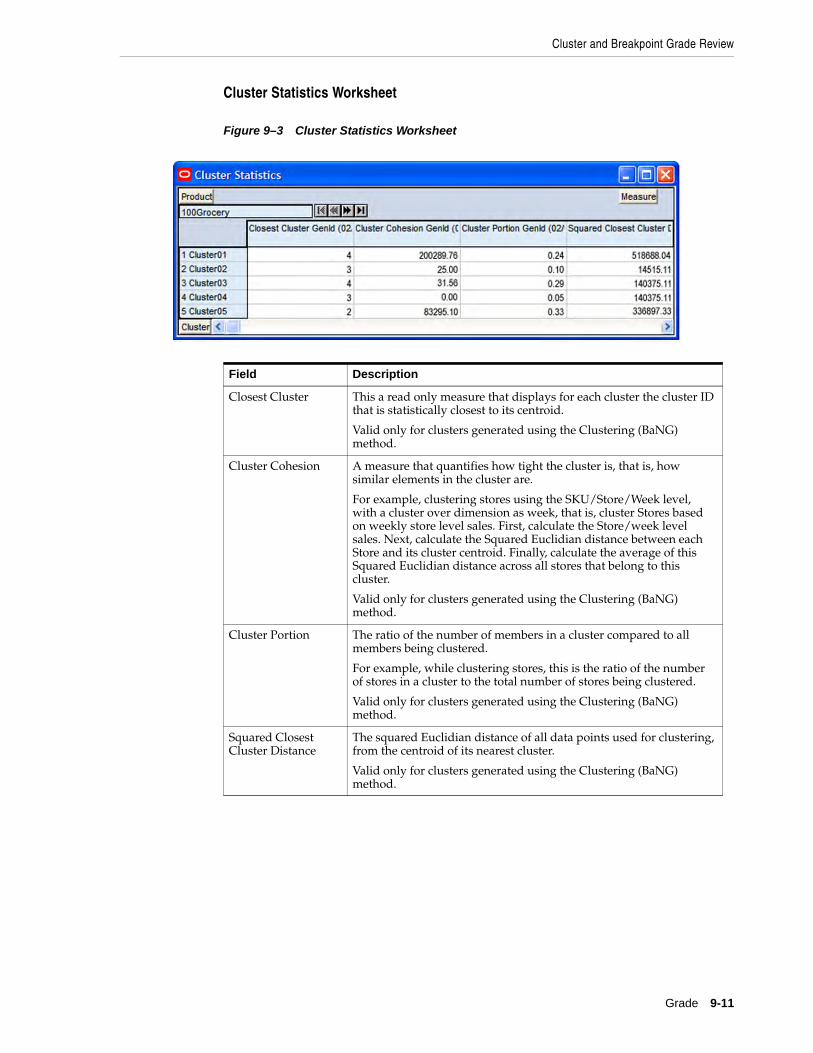
Cluster and Breakpoint Grade Review
Grade 9-11
Cluster Statistics Worksheet
Figure 9–3 Cluster Statistics Worksheet
Field Description
Closest Cluster This a read only measure that displays for each cluster the cluster ID that is statistically closest to its centroid.
Valid only for clusters generated using the Clustering (BaNG) method.
Cluster Cohesion A measure that quantifies how tight the cluster is, that is, how similar elements in the cluster are.
For example, clustering stores using the SKU/Store/Week level, with a cluster over dimension as week, that is, cluster Stores based on weekly store level sales. First, calculate the Store/week level sales. Next, calculate the Squared Euclidian distance between each Store and its cluster centroid. Finally, calculate the average of this Squared Euclidian distance across all stores that belong to this cluster.
Valid only for clusters generated using the Clustering (BaNG) method.
Cluster Portion The ratio of the number of members in a cluster compared to all members being clustered.
For example, while clustering stores, this is the ratio of the number of stores in a cluster to the total number of stores being clustered.
Valid only for clusters generated using the Clustering (BaNG) method.
Squared Closest Cluster Distance
The squared Euclidian distance of all data points used for clustering, from the centroid of its nearest cluster.
Valid only for clusters generated using the Clustering (BaNG) method.

Cluster and Breakpoint Grade Review
9-12 Oracle Retail Demand Forecasting User Guide for the RPAS Classic Client
Cluster Centroid Statistics Worksheet
Figure 9–4 Cluster Centroid Statistics Worksheet
Source Data Worksheet
Figure 9–5 Source Data Worksheet
Field Description
Cluster Centroid The average of the source data measure calculated across all cluster members; calculated by first aggregating the source data to the cluster on dimension for each member.
For example, while clustering stores using the SKU/Store/Week level sales history, the centroid is calculated as the average of the total historic sales of each store in the cluster.
Cluster Centroid to Average Ratio
The ratio of the cluster centroid, to the average of all data points used for the cluster run; calculated by first aggregating the source data to the cluster on dimension for each member.
For example, while clustering stores using the SKU/Store/Week level sales history, the Cluster to Average Ratio is calculated as the ratio of the Cluster Centroid to the average of the total historic sales for all stores being clustered.
Valid only for clusters generated using the Clustering (BaNG) method.
Field Description
Clustering Data Source The data used to generate the clusters or grades.

Cluster and Breakpoint Grade Review
Grade 9-13
Cluster Input Summary WorksheetThe Cluster Input Summary worksheet is a view to the settings used to generate the grades/clusters being reviewed in the workbook.
Figure 9–6 Summary Worksheet
Field Description
Cluster By Group Intersection
Displays Group By dimensions if selected during the cluster generation process. For example, while clustering stores by time period, such as quarter, the Cluster By Group is Qrtr (within the Calendar hierarchy). This means that clusters are generated one quarter at a time.
Cluster Method Displays the method used to generate the grades or clusters. Breakpoint or BaNG are valid methods.
Cluster Run Name Displays the name assigned by the user to the cluster run at the time the clusters were generated.
Dimension to Cluster Displays the Cluster Over dimension selected by the user during the cluster generation process.
The algorithm uses the positions in this dimension as the coordinates when clustering. Internally, data will be aggregated to this level before performing the clustering. For example, when using the SKU/Store/week level sales data to generate store clusters, the user has the option of specifying a dimension, such as Week, that will be used to aggregate the sales data to. In this case, the algorithm considers Store/Week positions and clusters stores based on their weekly sales.
A value will only be displayed in this field if the BaNG method was used.
Measure to Cluster Displays the measure selected as the clustering Data Source during the cluster generation process.
Number of Clusters Displays the number of clusters used during the cluster generation process.

Delete Clusters
9-14 Oracle Retail Demand Forecasting User Guide for the RPAS Classic Client
Delete ClustersThe Delete Cluster Run wizard allows you to delete clusters from the system based on Cluster Run Label and generation date (birth date).
Opening the Delete Cluster Run Template Wizard1. Within the Simple or Local Domain, select New from the File menu.
2. Select the Grade tab to display a list of workbook templates.
3. Select Delete Cluster Run. Click OK.
Delete Cluster Run WizardThe following steps outline the wizard process required to use the Delete Cluster Run wizard:
1. Select Cluster Run to Delete.
This wizard screen is a single select pick-list that includes the Cluster Run Label and the date/time stamp (birth date) for all cluster runs currently stored in the system. Select the Cluster Run Label to be deleted.
2. Select Next or Finish.
If Next is selected, Delete Cluster Run Succeeded is displayed once the cluster deletion process is completed.

A
Appendix: RDF Workbooks A-1
AAppendix: RDF Workbooks
This appendix provides a convenient reference of all the RDF workbooks and their respective tabs, worksheets, and measures by group:
■ Forecast Parameters Workbooks
■ Forecast Approval Workbook
■ Forecast Analysis Workbooks
■ Promotional Forecasting Workbooks
Forecast Parameters WorkbooksThis section lists the workbooks found in Chapter 4, "Setting Forecast Parameters," and their respective tabs, worksheets, and measures.
Forecast Administration WorkbookTable A–1 lists the tabs, worksheets, and measures for the Forecast Administration Workbook. For additional information, click any link to go to that section of the Oracle Retail Demand Forecasting User Guide for the RPAS Classic Client.

Appendix: RDF Workbooks A-2
Forecast Parameters Workbooks
Table A–1 Forecast Administration Workbook
Tabs Worksheets Measures
Basic Settings Workflow Tab Final Level Worksheet - Basic Settings
Default Approval Method
Default Source Level
Forecast Cycle
Forecast Start Date
Forecast Length
Next Run Date
Forecast Data Source
Final and Source Level Parameters Worksheet - Basic Settings
Forecast Data Source
Default History Start Date
Data Plan
Default Forecast Method
Seasonal Profile
Spreading Profile
Source Level Forecast Data Source
Source Level History Start Date
Advanced Settings Workflow Tab
Final Level Parameters Worksheet - Advanced Settings
Components - Baseline
Components - Baseline Interval
Components - Regular Price Lifts
Components - Promotional Lifts
Days to Keep Forecasts
Default Keep Last Changes
Generate Baseline Forecasts
Generate Cumulative Interval
Generate Intervals
Generate Methods
Generate Parameters
Interval Cap Lower Ratio
Interval Cap Upper Ratio
Item End Date Action
Like TS Duration (Periods)
Store Interim Forecast
Updating Last Week Forecast
Updating Last Week Forecast Number of Weeks

Appendix: RDF Workbooks A-3
Forecast Parameters Workbooks
Advanced Settings Workflow Tab
(continued)
Final and Source Level Worksheet - Advanced Settings
Bayesian Alpha (range (0, infinity))
Bayesian Cap Ratio
Crostons Min Gaps
DD Duration (weeks)
Default Moving Average Window Length
Fallback Method
Holt Min Hist (Periods)
Max Alpha (Profile) (range [0,1])
Max Alpha (Simple, Holt) (range [0,1])
Max Alpha (Winters) (range [0,1])
Max Gamma (Holt) (range [0,1])
Max Gamma (Winters) (range [0,1])
Seasonal Smooth Index
Trend Damping Factor (range [0,1])
Winters Min Hist (Periods)
Winters Mode
Winters Mode Impact on AutoES and Causal
Deseasonalized Demand Array
Causal Parameters Worksheet - Advanced Settings
Causal - Disable Seasonal Regression
Causal - Effects Only
Causal - Lift Estimate
Causal - Seasonal Baseline Selection Criteria
Causal - Smoothing Method
Causal Aggregation Profile
Causal Baseline Minimum Winters History Length
Causal Beta Scale
Causal Calculation Intersection
Causal Calculation Intersection Periodicity
Causal Capping Number
Causal Capping Ratio
Causal Data Source
Causal Higher Intersection
Causal Short Seasonal Threshold
Causal SLC - ROS
Causal Spread Profile
Disable Causal
Causal External Baseline
Minimum Causal Capping History (Periods)
Use Causal Capping
Regular Price Parameters Worksheet- Advanced Settings
Apply Regular Price Lift
Apply Regular Price Lift over Promotion
Regular Price Decaying Factor
Apply Regular Price Self Lift
Apply Regular Price Halo Lift
Apply Regular Price Cannibalization Lift
Regular Price Effective Periods
Price Elasticity Data Source
Table A–1 (Cont.) Forecast Administration Workbook
Tabs Worksheets Measures

Appendix: RDF Workbooks A-4
Forecast Parameters Workbooks
Forecast Maintenance WorkbookTable A–2 lists the tabs, worksheets, and measures for the Forecast Maintenance Workbook. For additional information, click any link to go to that section of the Oracle Retail Demand Forecasting User Guide for the RPAS Classic Client.
Forecast Like-Item, Sister-Store WorkbookTable A–3 lists the tabs, worksheets, and measures for the Forecast Like-item, Sister-Store Workbook. For additional information, click any link to go to that section of the Oracle Retail Demand Forecasting User Guide for the RPAS Classic Client.
Table A–2 Forecast Maintenance Workbook
Tabs Worksheets Measures
Basic Settings Workflow Tab Final and Source Level Worksheets - Basic Settings
Approval Method Override
Forecast Method Override
Winters Mode Override
Keep Last Changes Override
Optimal Source Levels
Pick Optimal Level
Source Level Override
Moving Average Window Length Override
Bayesian Alpha Override
Advanced Settings Workflow Tab
Final Advanced Parameter Worksheet
Forecast Start Date Override
Forecast End Date Override
History Start Date Override
Apply Regular Price Lift Override
Apply Regular Price Lift Over Promotion Override
Regular Price Decaying Factor Override
Apply Regular Price Self Lift Override
Apply Regular Price Halo Lift Override
Apply Regular Price Cannibalization Lift Override
Regular Price Effective Periods Override
Table A–3 Forecast Like-Item, Sister-Store Workbook
Tabs Worksheets Measures
Like-Item, Sister-Store Like-Item Worksheet Like SKU
Sister-Store Worksheet Sister-Store
Final Advance Parameter Worksheet
Adjustment Ratio
Forecast Start Date Override
Forecast End Date Override
History Start Date Override
Substitute Methods

Appendix: RDF Workbooks A-5
Forecast Approval Workbook
Product/Location Cloning Administration WorkbookTable A–4 lists the tabs, worksheets, and measures for the Product/Location Cloning Administration Workbook. For additional information, click any link to go to that section of the Oracle Retail Demand Forecasting User Guide for the RPAS Classic Client.
Forecast Approval WorkbookThis section lists the workbooks and wizards found in Chapter 5, "Generating and Approving a Forecast," and their respective tabs, worksheets, and measures.
WizardsThe Run Batch Forecast Workbook and Forecast Delete Workbook are wizards that execute functions for Forecast Approval.
Forecast Approval WorkbookTable A–5 lists the tabs, worksheets, and measures for the Forecast Approval Workbook. For additional information, click any link to go to that section of the Oracle Retail Demand Forecasting User Guide for the RPAS Classic Client.
Table A–4 Product/Location Cloning Administration Workbook
Tabs Worksheets Measures
Cloned History Adjustment Adjustment Parameters Worksheet
Cloned History Adjustment - Alpha (Range 0-1)
Cloned History Adjustment - Recent Sales Threshold
Cloned History Adjustment - Calculation Window Length
Product Cloning Product Cloning Worksheet Product Clones
Product Clone Contributions
Clone Product Adjustment Ratio
Location Cloning Location Cloning Worksheet Location Clones
Location Clone Contributions
Clone Location Adjustment Ratio
Clone Mask Clone Mask Worksheet Clone Mask

Appendix: RDF Workbooks A-6
Forecast Approval Workbook
Table A–5 Forecast Approval Workbook
Tabs Worksheets Measures
Approval Final Level Worksheet Adjusted Cumulative Interval
Adjusted Forecast
Approved Cumulative Interval
Approved Forecast
Approved System Forecast
Forecast Cumulative Interval
Forecast Interval
History Data
Interim Forecast
Last Approved Forecast
System Baseline
System Forecast
System Forecast without Regular Price Lift
Regular Price
Regular Price Halo Lift
Regular Price Halo Lift Ratio
Regular Price Cannibalization Lift
Regular Price Cannibalization Lift Ratio
Regular Price Self Lift
Regular Price Self Lift Ratio
Source Level Worksheet History Data
System Baseline
System Forecast
Approval Worksheet Approval Comment
Approval Date
Approved By
Manually Approved
Final or Source System Parameters Worksheet
Forecast Method Picked
System Generated Alpha
System Generated Level
System Generated Trend
Valid Forecast Run Worksheet
Final Level Run Flag

Appendix: RDF Workbooks A-7
Forecast Analysis Workbooks
Forecast Analysis WorkbooksThis section lists the workbooks found in Chapter 6, "Forecast Analysis Tools," and their respective tabs, worksheets, and measures.
Interactive Forecasting WorkbookTable A–6 lists the tabs, worksheets, and measures for the Interactive Forecasting Workbook. For additional information, click any link to go to that section of the Oracle Retail Demand Forecasting User Guide for the RPAS Classic Client.
Forecast Scorecard WorkbookTable A–7 lists the tabs, worksheets, and measures for the Forecast Scorecard Workbook. For additional information, click any link to go to that section of the Oracle Retail Demand Forecasting User Guide for the RPAS Classic Client.
Table A–6 Interactive Forecasting Workbook
Tabs Worksheets Measures
Interactive Forecasting Parameter Worksheet
Forecast Method
Forecast Picked Method
History Start Date
Forecast Start Date
Forecast End Date
Interactive Forecasting Worksheet
History Data
System Forecast
Table A–7 Forecast Scorecard Workbook
Tabs Worksheets Measures
Scorecard Error Measure Worksheet History Data for Forecast Window
Forecast Measures
Mean Error
Mean Absolute Error
Root Mean Squared Error
Mean Absolute Percentage Error
Percentage Absolute Error
Actuals versus Forecasts Worksheet
Actuals
History Data
Forecast Measures

Appendix: RDF Workbooks A-8
Promotional Forecasting Workbooks
Promotional Forecasting WorkbooksThis section lists the workbooks found in Chapter 7, "Promote (Promotional Forecasting)," and their respective tabs, worksheets, and measures.
Promotion Planner WorkbookTable A–8 lists the tabs, worksheets, and measures for the Promotion Planner Workbook Template. For additional information, click any link to go to that section of the Oracle Retail Demand Forecasting User Guide for the RPAS Classic Client.
Promotion Maintenance Workbook Table A–9 lists the tabs, worksheets, and measures for the Promotion Maintenance Workbook Template. For additional information, click any link to go to that section of the Oracle Retail Demand Forecasting User Guide for the RPAS Classic Client.
Table A–8 Promotion Planner Workbook
Tabs Worksheets Measures
Promotion Planner Promotion Planner Worksheet
Promotion Variables
Table A–9 Promotion Maintenance Workbook
Tabs Worksheets Measures
Promotion Maintenance Final PromoEffects Worksheet
System Calculated Effect
System Effect Override
Promo Effect Type

Appendix: RDF Workbooks A-9
Promotional Forecasting Workbooks
Promotion Effectiveness Workbook Table A–10 lists the tabs, worksheets, and measures for the Promotion Effectiveness Workbook Template. For additional information, click any link to go to that section of the Oracle Retail Demand Forecasting User Guide for the RPAS Classic Client.
Promotion Management Workbook Table A–11 lists the tabs, worksheets, and measures for the Promotion Management Workbook Template. For additional information, click any link to go to that section of the Oracle Retail Demand Forecasting User Guide for the RPAS Classic Client.
Table A–10 Promotion Effectiveness Workbook
Tabs Worksheets Measures
Promotion Effectiveness Promotion Variable/Effects Worksheets
Promotion Variables
Approved Effect
Simulated Effect
System Calculated Effect
Promotion Analysis Worksheet
History Data (the measure that represents Sales/Actuals)
System Forecast
Promotional Peak
Future Baseline
Future Forecast
Historical Baseline
Historical Forecast
Table A–11 Promotion Management Workbook
Tabs Worksheets Measures
Promotion Enable Promotion Enable Worksheet Enable Promotions
Accept Negative Lifts Accept Negative Lift Worksheet
Promotion Allow Negative Lift

Appendix: RDF Workbooks A-10
Promotional Forecasting Workbooks

Glossary-1
Glossary
Additive Seasonal Method
Also referred to as Additive Winters Model, this model is similar to the Multiplicative Winters model, but is it used when zeros are present in the data. This model adjusts the un-seasonalized values by adding the seasonal index for the forecast horizon.
Alert
A notice displayed to system users that a forecast value is above or below user-defined limits (an exception).
Alert Manager Window
A window that displays the alerts assigned to you. This dialog provides a list of all identified instances in which a monitored measure's values fall outside a set of defined limits. You may pick an alert from this list and have RCS automatically build a workbook containing the measure values that triggered the alert.
AutoES Method or Automatic Exponential Smoothing Method
RDF fits the sales data to a variety of exponential smoothing (time series) models of forecasting, and the best model is chosen for the final forecast. The candidate methods considered by AutoES are:
■ SimpleES
■ IntermittentES
■ TrendES
■ Multiplicative Seasonal
■ Additive Seasonal and SeasonalES
The final selection between the models is made according to a performance criterion (Bayesian Information Criterion) that involves a trade-off between the model's fit over the historic data and its complexity.
Note: With a few exceptions, this glossary contains definitions of terms specific to RDF. For further definitions of terms and concepts relating to the RPAS user interface, see the Oracle Retail Predictive Application Server Online Help or Oracle Retail Predictive Application Server User Guide.

Bayesian Method
Glossary-2 Oracle Retail Demand Forecasting User Guide for the RPAS Classic Client
Bayesian Method
Useful for short lifecycle forecasting and for new products with little or no historic sales data. The Bayesian method requires a product's known sales plan (created externally to RDF) and considers a plan's shape (the selling profile or lifecycle) and scale (magnitude of sales based on Actuals). The initial forecast is equal to the sales plan, but as sales information comes in, the model generates a forecast by merging the sales plan with the sales data. The forecast is adjusted so that the sales magnitude is a weighted average between the original plan's scale and the scale reflected by known history.
Causal Method
Causal is a forecasting method used for promotional forecasting and can only be selected if Promote is implemented. Typically, the Causal method is used at the Final Levels (that is, item/week/week). Causal uses a Stepwise Regression sub-routine to determine the promotional variables that are relevant to the time series and their lift effect on the series. AutoES utilizes the time series data and the future promotional calendar to generate future baseline forecasts. By combining the future baseline forecast and each promotion's effect on sales (lift), a final promotional forecast is computed.
Croston's Model of Exponential Smoothing
See IntermittentES or Intermittent Exponential Smoothing.
Curve
An optional automated predictive solution that transforms organization-level assortment plans into base-level weekly sales forecasts.
Exception
A forecast value that is greater than or less than a user-defined limit.
Exponential Smoothing
A form of a weighted moving average. Its weight declines in data exponentially. The most recent data is weighted more heavily. It requires a smoothing constant ( ). It ranges from 0 to 1 and is subjectively chosen.
Final Forecast Level
A low level in a hierarchy from which a forecast is generated, and at which approvals and data exports can be performed. Often, data from forecasts at a low level is insufficient to generate reliable forecasts without first aggregating the data to a higher level and then spreading the data back to the low level.
Forecast
In RDF, Forecast refers to RDF's statistical forecasting capabilities.
Forecast-Driven Planning
Planning that keys off of forecasts fed directly into a planning system. Connection to RDF is built directly into the business process supported by Oracle Retail Predictive Planning through an automatic approval of a forecast that is fed directly in the planning system. This allows you to accept all or part of Sales Value forecast. Once that decision is made, the balance of business measures are planned within Oracle Retail Predictive Planning.

Preprocessing
Glossary-3
Halo
Used to explain the bias shown by customers towards certain products because of a favorable experience with other products.
Holt's Model of Exponential Smoothing
See Trend Exponential Smoothing or TrendES.
Interactive Forecasting
A workbook in RDF that is used to simulate forecast by modifying parameters such as Forecast Method and History Start Date.
IntermittentES or Intermittent Exponential Smoothing
RDF fits the data to the Croston's model of exponential smoothing. This method should be used when the input series contains a large number of zero data points (that is, intermittent demand data). The original time series is split into a Magnitude and Frequency series, and then the SimpleES model is applied to determine level of both series. The ratio of the magnitude estimate over the frequency estimate is the forecast level reported for the original series.
Like Item or Like SKU
An item that is used as a model to forecast a new item introduction.
Lost Sales
Periods in sales data in which there was no inventory to meet consumer demand.
Measure
Any item of data that can be represented on a grid in worksheets.
Measure Description
The description of the measure that can be viewed in a workbook. This description may contain relationships and calculations.
Measure Function
Internal functions that can be used to simplify building calculations for a measure.
Measure Identifier
The combination of role, version, metric, and units that uniquely specifies a single measure.
Metric
A measure definition with the role, version, and units omitted.
Moving Average
For each period t, the moving average method takes the average of the periods from t-2 to t+2 as the smoothed baseline.
Multiplicative Seasonal
Also referred to as Multiplicative Winters Model, this model extracts seasonal indices that are assumed to have multiplicative effects on the un-seasonalized series.
Preprocessing
In RDF, Preprocessing refers to a module that processes data before forecasts are generated to adjust for situations, such as lost sales and unusually high demand.

Profile
Glossary-4 Oracle Retail Demand Forecasting User Guide for the RPAS Classic Client
Profile
Spreading ratios that are used in the Curve process. Typical profiles can include store participation, size distribution, and time (phase-to-week) profiles, as well as other information. Profiles are generated using historical data and phase definitions, based on your system configuration.
Profile Based
RDF generates a forecast based on a seasonal profile that can be created in Curve or a legacy system. Profiles can also be copied from another profile and adjusted. Using historic data and the profile, the data is de-seasonalized and then fed to the SimpleES method. The Simple forecast is then re-seasonalized using the profiles.
Profile Spread
Used at the final level to utilize a profile (either generated externally or with Curve) to determine the spreading ratios from the Source level forecast down to the Final level
Promote
Promote is an optional add-on automated predictive solution that allows you to incorporate the effects of promotional and causal events, such as radio advertisements and holiday occurrences, into your time series forecasts. The promotional forecasting process uses both past sales data and promotional information to forecast future demand.
Promotion Planning
A workbook template and simulation process used within the context of promotional forecasting. Promotion planning involves specifying whether the event status for a particular promotional variable is active (on) or inactive (off) for a specific product/location/calendar combination. When past promotional events are represented as accurately as possible, the modeling routine can more precisely detect correlation between event occurrences and changes in sales values.
Promotional Effectiveness
A workbook template used in the context of promotional forecasting. This workbook allows you to analyze the effects of promotions on items at both the micro and the macro level. What if analysis can also be performed on the results of promotional forecasts, as you can modify future and past promotional inputs, the system-estimated effects of promotions and the promotional forecasts themselves.
Promotional Forecasting
Promote's forecasting technique (also referred to as Causal forecasting) uses promotional factors and events to predict future demand. Promotion events are events; such as advertisements, holidays, competitor information, and other factors that affect the normal selling cycle for a business.
Promotion Group
A set of products or locations that are believed to exhibit similar effects during common causal events. Promotion groups should be established to maximize the number of time series for each group (so each promotional event can be evaluated from as many different observations as possible) while ensuring that each time series is affected by causal events to the same degree.
SeasonalES Method
A combination of several Seasonal methods. This method is generally used for known seasonal items or forecasting for long horizons. This method applies the Multiplicative

Wizard
Glossary-5
Seasonal model unless zeros are present in the data, in which case the Additive Winters model of exponential smoothing is used. If less than two years of data is available, a Seasonal Regression model is used. If there is too little data to create a seasonal forecast (in general, less than 52 weeks), the system selects from the SimpleES, TrendES, and IntermittentES methods.
Seasonal Regression
Seasonal Regression cannot be selected as a forecasting method, but it is a candidate model used when the SeasonalES method is selected. This model requires a minimum of 52 weeks of history to determine seasonality. Simple Linear Regression is used to estimate the future values of the series based on a past series. The independent variable is the series history one-year or one cycle length prior to the desired forecast period, and the dependent variable is the forecast. This model assumes that the future is a linear combination of itself one period before plus a scalar constant.
Simple/IntermittentES Method
A combination of the SimpleES and IntermittentES methods. This method applies the SimpleES model unless a large number of zero data points are present. In this case, the Croston's model is applied.
SimpleES or Simple Exponential Smoothing Method
RDF uses a simple exponential smoothing model to generate forecasts. SimpleES ignores seasonality and trend features in the demand data, and it is the simplest model of the exponential smoothing family. This method can be used when less than one year of historic demand data is available.
Simple Moving Average
See Moving Average.
Sister Store
A store that is used as a model to forecast a new store.
Source Level Forecast
The level at which the aggregate, more robust forecast is run.
Time Series
Set of evenly spaced numerical data obtained by observing response variable at regular time periods. This data is used to forecast based only on past values. It assumes that factors influencing past and present continues influence in future.
Training Window
The number of weeks of historical sales data to use in generating a forecast.
Trend Exponential Smoothing or TrendES
Also referred to as Holt's Model, RDF fits the data to the Holt model of exponential smoothing. The Holt model is useful when data exhibits a definite trend. This method separates out base demand from trend, and then provides forecast point estimates by combining an estimated trend and the smoothed level at the end of the series.
Wizard
A set of screens that guide you through the process of creating a new workbook or performing other actions in a solution by asking you various questions and having you select values.

Workbook
Glossary-6 Oracle Retail Demand Forecasting User Guide for the RPAS Classic Client
Workbook
The framework used for displaying data and user functions. Workbooks are task-specific and may contain one or more worksheets. Users define the format of their workbooks. Also see Workbook Template, Worksheet.
Workbook Template
The framework for creating a workbook. You build each new workbook from an existing workbook template, such as Pre-Season Financial Plan or Forecasting Administration. Several workbook templates are supplied with the Oracle Retail Predictive Solutions, and are available for selection when you choose File - New to create a new workbook.
Worksheet
A multidimensional spreadsheet used to display workbook-specific information. Worksheet data can also be displayed in chart format.