Capt Shedrick Bridgeforth

Air Force Cost Analysis

Agency (AFCAA)

Using Earned Value Data to Forecast the Duration and Cost of DoD Space

Programs

Disclaimer

The views expressed in this presentation are those of the

author and do not reflect the official policy or position of the

United States Air Force, Department of Defense, or the

United States Government. This material is declared a work

of the U.S. Government and is not subject to copyright

protection in the United States.

2

Overview

1. Summary

2. Background

3. Methodology

4. Results

5. Conclusion

3

Summary

AFCAA studied the accuracy of various cost estimating models for updating the estimate at completion (EAC) for space contracts

The Budgeted Cost of Work Performed (BCWP) based model was the most accurate

The BCWP model assumed the underlying duration estimate was accurate

Objective: Assess the accuracy of the duration method used in the AFCAA study and explore additional methods

Duration Results: 2.9 to 5.2% overall improvement (mean absolute percent error - MAPE)

Cost Results: 7.5% overall improvement (MAPE)

Background

EACBCWP = (MonthEst Completion – Monthcurrent) * BCWPBurn Rate

+ BCWPTo Date

[# of months remaining * earned value/month

+ earned value to date]

Duration: the Critical Path Method (CPM) is used to determine the duration of a project (contract) Contractor Reported Estimated Completion Date (ECD)

“Status quo”

Background

6

y = 72,401,283x - 45,653,892R² = 0.996

0

100

200

300

400

500

600

700

800

900

0 2 4 6 8 10 12

Millio

ns

Months

BCWP vs. Time

Background

AFCAA Study (Keaton, 2014)

Why Improve Accuracy?

Improve the accuracy of the duration estimate in order

to:

Improve the accuracy of the cost estimate (earlier)

Detect schedule issues sooner (take corrective action)

Why is accuracy important?

Underestimating – increased portfolio risk

Overestimating – opportunity cost

May not prevent further cost/schedule growth: earlier

detection should lead to better decisions and more accurate

budget inputs

Data Source: EVM-Central Repository

Program Data Points

Advanced Extremely High Frequency Satellite (AEHF) 148

Evolved Expendable Launch Vehicle (EELV) 12

Family of Beyond Line-of-Sight Terminals (FAB-T) 77

Military GPS User Equipment (MGUE) 31

Mobile User Objective System (MUOS) - Navy 55

Next Generation Operational Control System (GPS OCX) 21, 24, 61

NAVSTAR Global Positioning System (NAVSTAR GPS) 68, 70, 71

Space-Based Infrared System High Component (SBIRS High) 219

Wideband Global SATCOM (WGS) 43, 87

Methodology

1. Status Quo: reported duration (base case)

2. IMS: Earned Value Forecasting (EVM and Earned

Schedule Index based) + Time Series Analysis

3. Linear Regression

4. Kalman filter Earned Value Method (KEVM)

5. IDE: Integrated Master Schedule Analysis

(Independent Duration Estimate) + Time Series

Analysis

Status Quo

Contractor Performance Report Planned Duration (CPR

PD)

Based on the critical path method

The duration estimate is calculated with the:

Contract Start Date

Estimated Completion Date (ECD)

Earned Value Forecasting

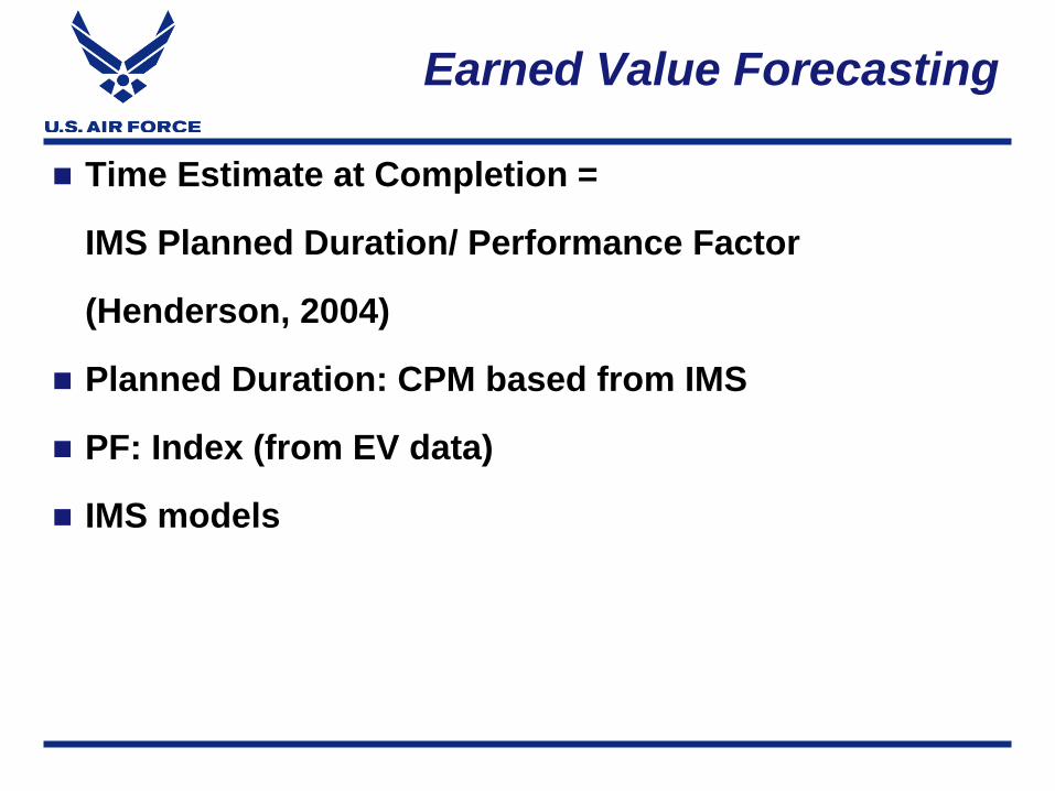
Time Estimate at Completion =

IMS Planned Duration/ Performance Factor

(Henderson, 2004)

Planned Duration: CPM based from IMS

PF: Index (from EV data)

IMS models

Performance Factors

Name Reported Time Series

Baseline Execution Index BEI BEI (T.S.)

Schedule Performance Index SPI SPI (T.S.)

Cost Performance Index CPI CPI (T.S.)

Earned Schedule SPI SPI(t) SPI(t) (T.S.)

Schedule Cost Index SPI*CPI SPI (T.S.)*CPI (T.S.)

Schedule Cost Index (ES) SPI(t)*CPI SPI(t) (T.S.) *CPI (T.S.)

Enhanced Schedule Cost Index BEI*CPI*SPI BEI*CPI (T.S.)*SPI (T.S.)

Enhanced Schedule Cost Index (ES) BEI*CPI*SPI(t) BEI (T.S.)*CPI (T.S.)*SPI(t) (T.S.)

Enhanced CPI BEI*CPI BEI (T.S.)*CPI (T.S.)

Enhanced SPI BEI*SPI BEI (T.S.)*SPI (T.S.)

Enhanced SPI(t) BEI*SPI(t) BEI (T.S.)*SPI(t) (T.S.)

BEI = cumulative # of baseline tasks completed / cumulative # of baseline tasks scheduled for

completion

[used NASA’s Schedule Test and Assessment Tool (STAT)]

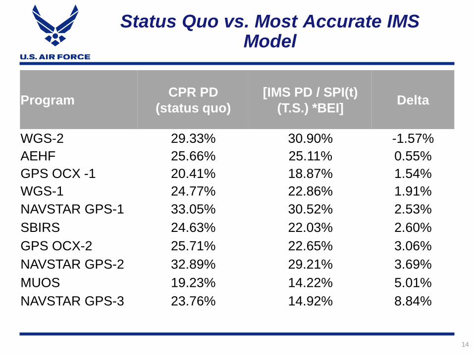
Status Quo vs. Most Accurate IMS Model

ProgramCPR PD

(status quo)

[IMS PD / SPI(t)

(T.S.) *BEI]Delta

WGS-2 29.33% 30.90% -1.57%

AEHF 25.66% 25.11% 0.55%

GPS OCX -1 20.41% 18.87% 1.54%

WGS-1 24.77% 22.86% 1.91%

NAVSTAR GPS-1 33.05% 30.52% 2.53%

SBIRS 24.63% 22.03% 2.60%

GPS OCX-2 25.71% 22.65% 3.06%

NAVSTAR GPS-2 32.89% 29.21% 3.69%

MUOS 19.23% 14.22% 5.01%

NAVSTAR GPS-3 23.76% 14.92% 8.84%

14

IMS Analysis – Independent Duration Estimate (IDE)

Lofgren (2014)

Independent Duration Estimate (IDE)

Schedule slip

Slip = Max (Current Finish – Baseline Finish – Total

Slack)

IDE = Schedule slip + baseline duration estimate

Time Forecast = IDE/PF

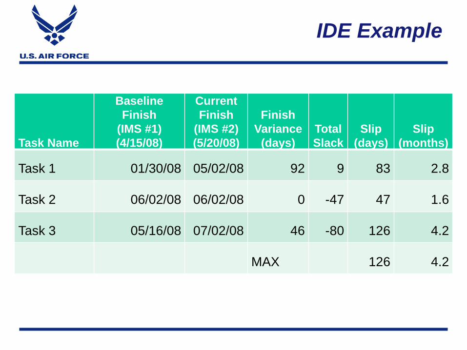
IDE Example

Task Name

Baseline

Finish

(IMS #1)

(4/15/08)

Current

Finish

(IMS #2)

(5/20/08)

Finish

Variance

(days)

Total

Slack

Slip

(days)

Slip

(months)

Task 1 01/30/08 05/02/08 92 9 83 2.8

Task 2 06/02/08 06/02/08 0 -47 47 1.6

Task 3 05/16/08 07/02/08 46 -80 126 4.2

MAX 126 4.2

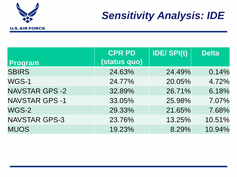
Sensitivity Analysis: IDE

Program

CPR PD

(status quo)

IDE/ SPI(t) Delta

SBIRS 24.63% 24.49% 0.14%

WGS-1 24.77% 20.05% 4.72%

NAVSTAR GPS -2 32.89% 26.71% 6.18%

NAVSTAR GPS -1 33.05% 25.98% 7.07%

WGS-2 29.33% 21.65% 7.68%

NAVSTAR GPS-3 23.76% 13.25% 10.51%

MUOS 19.23% 8.29% 10.94%

Revisit Original Study

AFCAA Study (Keaton, 2014)

Cost Estimate Accuracy

Applying duration estimates to BCWP model

EAC Reported

BCWP 1: [CPR PD and actual time] (Keaton, 2014)

BCWP 2: [IMS PD / (SPI(t)*CPI) and actual time]

Simplicity, lack of data for other methods (IDE, BEI)

Added out of sample contracts:

EELV (Evolved Expendable Launch Vehicle) (Production)

MGUE (Military GPS User Equipment) (RDT&E, Production)

FAB-T (Family of Beyond Line-of-Sight Terminals) (RDT&E)

MUOS (Mobile User Objective System) (RDT&E)

GPS OCX (Next Generation Control Segment) (Phase B)

(RDT&E)

Cost Estimate Accuracy

Metric EAC BCWP1 BCWP2

EAC

Delta

BCWP1

Delta

MAPE 25.3% 25.8% 17.8% 7.5% 8.0%

Median APE 28.0% 22.3% 14.3% 13.7% 8.1%

MAPE (0 to 70%) 33.3% 27.2% 20.9% 12.4% 6.1%

MAPE (20 to 70%) 28.6% 22.3% 16.3% 12.8% 7.4%

MAPE – mean absolute percent error

APE - absolute percent error

Accuracy - All Contracts

0%

10%

20%

30%

40%

50%

60%

10% 20% 30% 40% 50% 60% 70% 80% 90% 100%

Ab

so

lute

Perc

en

t E

rro

r fr

om

Fin

al

EA

C

Mean Absolute Percent Error vs. % Complete

EAC

BCWP1

BCWP2

Dollars & Sense

Get your Billions Back America!

Not really… This next analysis is NOT Savings or Potential Realizable Savings

% error converted to dollars based on the portfolio cost ($25.1B in FY15$)

Comparison purposes over time

Not cumulative

[MAPEs*$25.1B = Estimating Error ($B)]

[10% intervals]

Cost Estimate Error ($)

24

10% 20% 30% 40% 50% 60% 70% 80% 90% 100%

EAC $12.1 $11.8 $10.4 $9.3 $7.5 $5.5 $3.8 $1.9 $0.5 $0.2

BCWP1 $11.3 $9.4 $8.8 $6.9 $5.1 $4.5 $4.7 $4.9 $4.9 $4.5

BCWP2 $11.8 $8.4 $6.0 $4.7 $3.6 $2.7 $2.9 $2.7 $2.4 $1.9

$-

$2.0

$4.0

$6.0

$8.0

$10.0

$12.0

$14.0

Err

or

($B

FY

15

) fr

om

Fin

al E

AC

Estimate Error ($B FY15) vs. % Complete

Average Estimate Error

25

Average Error (in $B FY15)

EAC $6.3

BCWP1 $6.5

BCWP2 $4.5

$-

$1.0

$2.0

$3.0

$4.0

$5.0

$6.0

$7.0

Conclusions

Improved the accuracy of estimates: Improved the accuracy of the cost estimate (EAC)

[earlier]

More accurate inputs into the budget

Detect schedule issues sooner (take corrective action)

Why is accuracy important? Underestimating – increased portfolio risk, a “tax” on

other programs

Overestimating – opportunity cost

May not prevent further cost/schedule growth: earlier detection could lead to better decisions and resource allocation

Limitations

Small sample size (7, 10, & 15)

Some contracts did not have data for calculating IDEs

or BEIs

More research is needed

Questions?

??

Beep...Beep...Beep...

Backup Slides

Earned Schedule

Lipke, 2011

Linear Regression (Smoker)

Regress BAC (Y) by Months (X)

BCWP (Y) by Months (X)

Set equations equal to each other

(1) BCWP coefficient*Months + BCWP intercept =

BAC intercept + BAC coefficient*Months

(2) Months = BAC intercept – BCWP intercept

(BCWP coefficient – BAC coefficient)

BAC – Budget at Completion

BCWP – Budgeted Cost of Work Performed

Linear Regression

y = 10,245,599.65x - 15,859,909.69R² = 0.98

y = 761,814.97x + 128,341,631.95R² = 0.67

0

20,000,000

40,000,000

60,000,000

80,000,000

100,000,000

120,000,000

140,000,000

160,000,000

0 1 2 3 4 5 6 7 8 9 10 11 12 13 14 15 16

BCWP

BAC

BCWP Predicted

BAC Predicted

Linear (BCWP)

Linear (BAC)

761,814.97x + 128,341,631.95 = 10,245,599.65x - 15,859,909.69

Months = 15.2

Kalman filter Earned Value Method (KEVM)

Recursive learning cycle of the Kalman filter (Kim, 2013)

x = state variables, P = error covariance variables

Kalman filter Earned Value Method (KEVM)

(Kim and Reinschmidt, 2011)

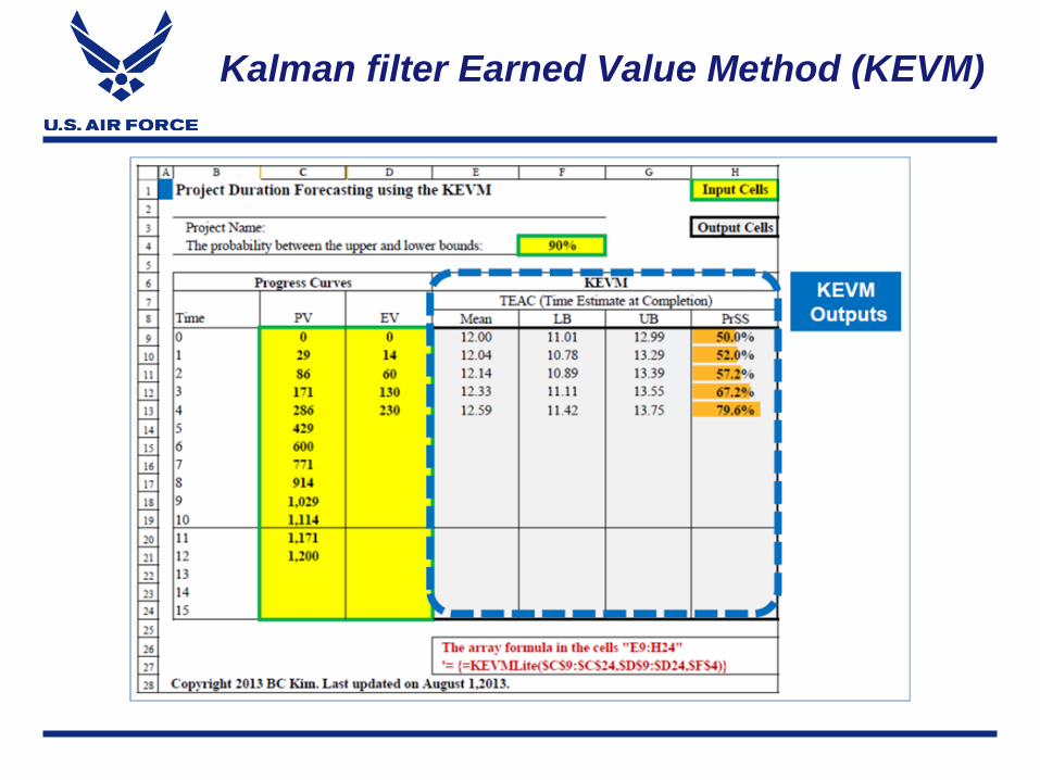
Kalman filter Earned Value Method (KEVM)

36

Contract Final Duration MAPE Final EAC MAPE

CPR PD SPI(t)* CPI EAC BCWP BCWP

GPS MUE-3 22.70% 21.00% 31.60% 22.70% 8.70%

AEHF* 25.70% 23.20% 23.70% 16.30% 11.70%

FAB-T 8.30% 3.60% 25.90% 21.30% 12.20%

GPS OCX-1 20.40% 19.90% 13.90% 13.10% 12.40%

EELV 5.70% 9.00% 23.70% 16.10% 14.40%

GPS OCX-2 22.70% 22.00% 15.80% 17.90% 15.00%

WGS-1 24.80% 20.80% 17.60% 52.20% 17.00%

WGS-2 29.30% 36.20% 2.70% 32.00% 17.20%

MGUE* 42.10% 27.90% 28.00% 30.80% 18.10%

MUOS-2 8.60% 9.60% 22.50% 19.60% 18.50%

GPS MUE-1 33.00% 25.00% 35.60% 26.90% 19.90%

GPS OCX B* 23.10% 16.30% 37.30% 27.60% 20.20%

GPS MUE-2 32.80% 28.50% 37.90% 24.80% 22.00%

MUOS-1 20.30% 34.40% 24.20% 35.10% 28.80%

SBIRS* 24.70% 24.20% 38.80% 30.20% 30.40%

*Not 100% complete

Literature Review

1991 Cancellation of A-12 Avenger ignited EVM research

David Christensen – EAC (1993 & more)

Walt Lipke – Earned Schedule and SPI(t) (2003 & more)

Kym Henderson – EAC and Time EAC with SPI(t) (2004)

(shorter contracts and non DoD)

Forecasting: Methods and Applications (Makridakis,

Wheelwright, & Hyndman) (1998)

Roy Smoker - Regression (2011)

B.C. Kim - Kalman Filter Forecasting Method (2007)

Eric Lofgren – Improving the schedule estimate with the IMS

(2014)