USER�s Manual

Release 22c June 2005

Klaus Stüben Tanja Clees

Fraunhofer Institute SCAI Schloss Birlinghoven

D-53754 St. Augustin, Germany

Service & Technical Support samg@scai.fraunhofer.de

Document version 22c-1.1

2

Contents

1 Introduction and Overview ...................................................................................................................... 4 1.1 Review of SAMG................................................................................................................................. 4

1.1.1 Hierarchical solvers...................................................................................................................... 4 1.1.2 Algebraic multigrid (AMG)............................................................................................................ 4 1.1.3 The SAMG package..................................................................................................................... 5

1.2 Overview of this manual...................................................................................................................... 5 1.3 Additional documents and support...................................................................................................... 6

2 Background Information.......................................................................................................................... 7 2.1 The structure of SAMG ....................................................................................................................... 7 2.2 The performance of SAMG ................................................................................................................. 8 2.3 Features, an overview......................................................................................................................... 9

2.3.1 General features .......................................................................................................................... 9 2.3.2 More specific features................................................................................................................ 10

3 Solution Approaches ............................................................................................................................. 12 3.1 Variable-based approach.................................................................................................................. 12 3.2 Unknown-based approach ................................................................................................................ 13 3.3 Point-based approaches ................................................................................................................... 13

4 Data Structure......................................................................................................................................... 15 4.1 The linear system of equations ......................................................................................................... 15 4.2 Additional data and requirements in case of coupled systems......................................................... 16

5 Basic Aspects and Conventions........................................................................................................... 17 5.1 Naming convention for parameters................................................................................................... 17 5.2 Multi-purpose use of single parameters............................................................................................ 17

5.2.1 Integers ...................................................................................................................................... 17 5.2.2 Reals .......................................................................................................................................... 17

5.3 Classes of SAMG parameters........................................................................................................... 18 5.3.1 List parameters (primary parameters) ....................................................................................... 18 5.3.2 Hidden parameters .................................................................................................................... 18 5.3.3 Accessing hidden parameters via set- and get-routines............................................................ 18 5.3.4 Alternative set- and get-routines (for Fortran users only) .......................................................... 19

5.4 Automatic memory management by SAMG...................................................................................... 20 5.5 Providing grid coordinates to SAMG (optional)................................................................................. 21

6 Calling Sequence: The Primary Parameters........................................................................................ 22 6.1 Passing the linear system of equations ............................................................................................ 22 6.2 First approximation and stopping criterion ........................................................................................ 23 6.3 Distinguishing scalar and coupled systems ...................................................................................... 23 6.4 Selecting the solution approach........................................................................................................ 24

6.4.1 The solution strategy.................................................................................................................. 24 6.4.2 The smoothing strategy ............................................................................................................. 25 6.4.3 Specifying a primary matrix (for point-based approaches) ........................................................ 26 6.4.4 Specifying details of interpolation (all solution approaches)..................................................... 27 6.4.5 Summary.................................................................................................................................... 29

6.5 Selecting SAMG�s cycling process ................................................................................................... 31 6.6 General control switch....................................................................................................................... 32

6.6.1 Repeated calls to SAMG............................................................................................................ 32 6.6.2 Memory extension switch........................................................................................................... 33 6.6.3 Selecting default values for certain hidden parameters............................................................. 33 6.6.4 Norms and scratch files ............................................................................................................. 34 6.6.5 Displaying histories of errors...................................................................................................... 34

6.7 Initial dimensioning............................................................................................................................ 35 6.8 Checking and printing ....................................................................................................................... 36

6.8.1 Input matrix checking ................................................................................................................. 36 6.8.2 Print output during the solution phase ....................................................................................... 36 6.8.3 Print output during the setup phase........................................................................................... 37

6.9 Output parameters ............................................................................................................................ 38

3

7 Hidden Parameters................................................................................................................................. 39 7.1 Parameters related to SAMG�s setup phase..................................................................................... 40

7.1.1 Threshold values for defining strong connectivity...................................................................... 40 7.1.2 Treatment of positive off-diagonal matrix entries in coarsening ................................................ 41 7.1.3 Standard and aggressive coarsening ........................................................................................ 42 7.1.4 Exceptional situations ................................................................................................................ 42 7.1.5 Termination criteria for the coarsening process......................................................................... 43 7.1.6 Interpolation ............................................................................................................................... 44 7.1.7 Special parameters for point-based approaches....................................................................... 45 7.1.8 The Galerkin coarse-level matrices ........................................................................................... 46 7.1.9 Truncation features .................................................................................................................... 46

7.2 Parameters related to SAMG�s solution phase................................................................................. 47 7.2.1 The smoothing process.............................................................................................................. 47 7.2.2 The coarsest-level solver ........................................................................................................... 49

7.3 Further parameters ........................................................................................................................... 51 7.3.1 Re-directing and limiting I/O....................................................................................................... 51 7.3.2 Default values for various primary parameters .......................................................................... 51 7.3.3 Some special parameters .......................................................................................................... 52 7.3.4 Setting hidden parameters via the default switch n_default ...................................................... 53

8 Special Options in Using SAMG ........................................................................................................... 54 8.1 OpenMP parallelization ..................................................................................................................... 54 8.2 Stopping criteria for the iterative solution process ............................................................................ 55

8.2.1 Convergence criteria.................................................................................................................. 56 8.2.2 Safety checks............................................................................................................................. 57

8.3 Forcing special variables into coarse or fine levels........................................................................... 59 8.3.1 Explicitly forcing variables to exist on all coarse levels ............................................................. 59 8.3.2 Explicitly forcing variables to remain only on the finest level..................................................... 60 8.3.3 Additional features ..................................................................................................................... 62

8.4 Making repeated use of SAMG�s setup phase.................................................................................. 63 8.4.1 Manual control ........................................................................................................................... 63 8.4.2 Automatic control ....................................................................................................................... 64

8.5 Special case: one-level methods ...................................................................................................... 66 8.6 Optimizing SAMG's performance (under construction)..................................................................... 67

8.6.1 The main control parameter....................................................................................................... 67 8.6.2 Details of optimization process .................................................................................................. 68

8.7 Controling very specific output (involving files) ................................................................................. 69 8.7.1 Specifying file format.................................................................................................................. 69 8.7.2 Displaying error histories ........................................................................................................... 69 8.7.3 Dumping matrices to disk........................................................................................................... 70 8.7.4 Writing intermediate approximations (frames) to disk ............................................................... 70 8.7.5 Writing coarsening pattern to disk ............................................................................................. 71

9 Special Interfaces................................................................................................................................... 72 9.1 Alternative interfaces to call SAMG ................................................................................................. 72

9.1.1 Simplified interfaces (input via files) .......................................................................................... 72 9.1.2 An AMG1R5-like interface ......................................................................................................... 74

9.2 User interfaces .................................................................................................................................. 76 9.2.1 Interface to the coarsest-level solver ......................................................................................... 76 9.2.2 Interface to check the input matrix ............................................................................................. 78 9.2.3 Interface to a user's license checker.......................................................................................... 79 9.2.4 Interface for getting current cycle number and residual ............................................................ 79

10 Code Numbers of Errors and Warnings ........................................................................................... 80 11 What is New in this Release? ............................................................................................................ 82

11.1 Bug fixes ........................................................................................................................................ 82 11.2 New features.................................................................................................................................. 82 11.3 New default values ........................................................................................................................ 82 11.4 Other.............................................................................................................................................. 82

12 References........................................................................................................................................... 83 13 Index..................................................................................................................................................... 84

4

1 Introduction and Overview 1.1 Review of SAMG 1.1.1 Hierarchical solvers The efficient numerical solution of large systems of discretized elliptic partial differential equations (PDEs) requires hierarchical algorithms which ensure a rapid reduction of both short and long range error compo-nents. A breakthrough, and certainly one of the most important advances during the last three decades, was due to the multigrid principle. Any corresponding method operates not only on the given discretization grid but rather on a hierarchy of grids, defined a priori by coarsening the given grid in a geometrically natural way (�geometric� multigrid). Since the early nineties, there is a strong increase of interest in algebraically oriented hierarchical methods which construct a reasonable hierarchy automatically, based on algebraic information (explicitly or implicitly contained in the discretization matrix) rather than grid information. One reason for this is certainly the in-creasing geometrical complexity of applications which, technically, limits the immediate use of geometric multigrid. Another reason is the steadily increasing demand for efficient �plug-in� solvers which can be inte-grated into existing software packages without the need of a complete code re-structuring. In particular in commercial codes, this demand is driven by increasing problem sizes which clearly exhibit the limits of the classical one-level solvers still used in most packages. Millions of degrees of freedom in the underlying nu-merical models require hierarchical approaches for an efficient solution. 1.1.2 Algebraic multigrid (AMG) The first hierarchical, matrix-based approach was algebraic multigrid (AMG) which extends the classical ideas of geometric multigrid (based on smoothing and coarse-grid correction) to certain classes of linear systems of equations. Rather than on a hierarchy of grids, AMG operates on a hierarchy of increasingly smaller linear systems of equations which is constructed fully automatically. In particular, the construction of operators (matrices) used to transfer information between different levels (restriction of residuals and interpolation of corrections) is based on matrix entries, and matrices on coarser levels are computed based on the so-called Galerkin principle (Galerkin matrices). This automatism is the major reason for AMG's flexibility in adapting itself to specific requirements of the problem to be solved and is the main reason for its robustness in solving large classes of problems despite using very simple smoothers. Although the origin of AMG dates back to the early eighties [1-5], it still provides one of the most attractive algebraic approaches. However, substantial research on AMG is still ongoing, mainly aiming at extending its range of applicability. Major research is focusing on applications involving coupled systems of PDEs for which a robustness and efficiency has not yet been reached to the same extent as for scalar PDEs. Nevertheless, substantial progress has been achieved and further advances are to be expected in the near future. For some review on the state of the art, we refer to [8]. A detailed introduction to AMG is presented in [7], results on its parallelisation are found in [9]. Regarding techniques and applications for selected coupled systems of PDEs, see [14].

5

1.1.3 The SAMG package SAMG, written in FORTRAN90, is based on an AMG approach which, by our experience, has turned out to be very flexible, robust and efficient in practice. Essential components of SAMG have been implemented already in the code RAMG [7], which is a successor of the original (public domain) code AMG1R5, described in [3]. Compared to RAMG, however, SAMG is much more general. In particular, SAMG can be applied to both scalar and coupled systems of �elliptic� PDEs. From the user�s point of view, SAMG is a �plug-in� solver. Essentially, just the (sparse) linear system of equations to be solved,

Au=f, has to be passed to SAMG. In general, no information regarding the shape of the domain or the structure of the underlying grid needs to be provided. Thus, besides its robustness and efficiency, the main practical advantage of SAMG is that it can directly be applied to solve certain classes of PDEs on unstructured meshes, both in 2D and 3D. Moreover, SAMG can even be applied to problems without any geometric background, provided that the underlying matrices are of a �similar type� as the ones arising from elliptic PDEs. 1.2 Overview of this manual The SAMG package is considerably more complex than a standard numerical solver. SAMG is actually not just a fixed solver but rather a complete multi-level environment. This implies that its use is not as straightforward as that of a classical solver. In order to take full advantage of the various features of SAMG, it is very helpful to have some basic understanding of the multi-level principle in general, and SAMG�s way of operation in particular. Most basic aspects are introduced in Section 2. A brief introduction to the solution approaches provided by SAMG and the underlying data structures are given in Section 3 and 4, respectively. Various basic aspects and conventions are summarized in Section 5. Among others, this includes a description of SAMG's parameter classes, the automatic memory management, as well as the option to provide grid coordinates to SAMG. The main user interface to SAMG (calling sequence) is described in detail in Section 6. We call the corresponding parameters �primary parameters�. Besides these primary parameters, there are various other ones which are hidden to the user, most of which are explained in Section 7. Under most conditions, the user is not supposed to access these parameters. In critical situations, however, it may be necessary to tune particular hidden parameters more carefully in order to achieve best performance of SAMG. In this case, the user might need to modify one or more of the hidden parameters. How to achieve this, is described in Section 5.3. Section 8 describes various special options in using SAMG such as its OpenMP parallelization, a variety of termination criteria for the iterative process, ways of how to force particular variables into coarse or fine levels (in particular, how to set up some kind of Schwarz alternating process), ways to use SAMG as a one-level solver, a prototype routine to automatically reuse SAMG decompositions, and more. Available user interfaces can be found in Section 9. In case SAMG terminates with an error or a warning, we refer to Section 10 for a list of error codes. In Section 11 we summarize changes between the SAMG Release 21 and 22.

6

In order to draw the reader�s attention, we use the following symbols for highlighting:

Non-critical information on particular aspects of SAMG.

Attention: Critical aspects and/or important remarks.

Stop and read: Particularly critical aspects and/or important remarks.

Under construction: This symbol marks features which are either not yet installed in the current release or which are in a test phase and not yet supposed to be selected by the average user.

Colored text is used for highlighting as follows: • Generally, the color red highlights important aspects, remarks and definitions. • Examples, computer output, program code, program and file names are printed in blue. • Text printed in green refers to options or features which are not meant to be used by an average user. Finally, text printed on a yellow background marks, for instance, typical default/standard parameter settings or directs the readers attention to standard situations or procedures. 1.3 Additional documents and support Additional SAMG-related documents, papers and reports are available and can be downloaded from our Web page http://www.scai.fraunhofer.de/samg.htm. Regarding technical support, questions, suggestions and the like, please contact us via our service e-mail,

samg@scai.fhg.de. Please note that this e-mail addresses our whole SAMG-Team. Therefore, it should only be used for moderately sized e-mails, not to send large amounts of data.

7

2 Background Information As mentioned before, SAMG is not just a fixed solver but rather a complete multi-level environment. Consequently, its optimal use requires some basic understanding of the multi-level principle in general, and SAMG�s way of operation in particular. In contrast to a classical numerical solver, SAMG takes specific characteristics of a given linear system of equations into account. For instance, SAMG needs to distinguish between problems corresponding to discretized scalar or coupled systems of PDEs. Corresponding information has to be provided to SAMG. In this section, we summarize some basic facts on SAMG. We refer the interested reader to [7] where details on AMG can be found. 2.1 The structure of SAMG A call to SAMG invokes a two-part process. The first part, a fully automatic setup phase, recursively performs four steps: 1. The connectivity of the current matrix is analyzed. The

purpose is to separate the non-zero couplings into �strong� and �weak� ones.

2. Based on some splitting process, the next coarser level (subset of variables) is now constructed: On the current level, the total set of variables is split into a subset of variables which remain alive (C-variables) and the complementary set (F-variables).

3. Guided by the knowledge of strong couplings, the transfer operators (interpolation and restriction) are computed. (Generally, restriction is the transpose of interpolation.)

4. The coarse-level matrix is computed, based on the so-called Galerkin principle (Galerkin matrix).

The individual steps of SAMG�s setup phase are controlled by various parameters some of which require a fairly detailed understanding of the whole coarsening process. These parameters are hidden from the normal user of SAMG ("hidden parameters", see Section 5.3). Only rarely, the user might need to explicitly adjust one or more of the hidden parameters. Note: For brevity, we sometimes call the result of this phase the �decomposition�, although it has not much in common with what is normally called a decomposition. The second part, the solution phase, just uses the resulting components in order to perform normal multigrid cycles (iterations) until a desired level of tolerance is reached. As with any other multigrid method, SAMG�s solution phase consists of three algorithmical components:

• smoothing on all but the coarsest level (eg, by plain Gauss-Seidel relaxation), • data transfer between levels (interpolation and restriction), • solution on the coarsest level (which should be accurate up to at least 1-2 digits).

Coarsening

Interpolation

Galerkin operator

Coarse enough?

Multigrid cycling

Converged?

Setup phase

Solution phase

no

yes

no

Return

Call

Matrix analysis

yes

8

These components (which are also partly controlled by hidden parameters) are �combined� to so-called multigrid cycles which are then used for the final iteration process. There are essentially four types of cycle, referred to as V-, F-, W- and WW-cycle, which differ only in the extent to which they approximate the corresponding two-level cycle. That is, these cycles are increasingly more �robust� but also increasingly more expensive (the WW-cycle being the most expensive one). In practice, the cheap V-cycle is generally the best and most efficient choice. 2.2 The performance of SAMG Compared to geometric multigrid, the flexibility of SAMG and its simplicity of use, of course, have a price. The extra overhead caused by the setup phase is one reason for the fact that SAMG is usually somewhat less efficient than geometric multigrid (if applied to problems for which geometric multigrid can be applied efficiently). Another reason is that SAMG's hierarchical components can, generally, not be expected to be optimal. In fact, they will always be constructed on the basis of compromises between numerical work and overall efficiency. Nevertheless, as a rough guide line, the computational cost of SAMG's solution phase (ignoring the setup cost) is typically comparable to the solution cost of a robust geometric multigrid solver, if applied to standard elliptic test problems. However, SAMG should not be regarded as a competitor of geometric multigrid. The strengths of SAMG are its robustness, its applicability in complex 2D and 3D geometric situations and its applicability to even solve certain problems which are out of the reach of geometric multigrid, in particular, problems with no geometric or continuous background at all (as long as the given matrix is similar to those arising in PDE applications). That is, SAMG provides an attractive multi-level variant whenever geometric multigrid is either too difficult to apply or cannot be used at all. In such cases, SAMG should be regarded as an efficient alternative to standard numerical solvers such as conjugate gradient accelerated by classical one-level preconditioners. As mentioned before, substantial research and development on algebraic multigrid is still ongoing and many problems cannot yet be tackled efficiently. However, SAMG�s range of applicability is growing steadily, and its robustness and efficiency are continuously being enhanced. If applied in mature cases, in contrast to any one-level method, SAMG has a convergence behavior which does virtually not depend on the size of the given problem. Consequently, SAMG becomes the more attractive, the larger a given problem is. Remark: Originally, SAMG has been developed as a stand-alone iterative solver. Practical experience, however, has clearly shown that SAMG is also a very good preconditioner, much better than standard (one-level) preconditioners. Heuristically, the major reason is due to the fact that SAMG, in contrast to any one-level preconditioner, aims at the efficient reduction of all error components, short-range as well as long-range. Consequently, highest efficiency is typically obtained if multigrid cycling is accelerated by standard methods such as conjugate gradient (CG), BiCGstab or GMRES all of which are included in SAMG.

9

2.3 Features, an overview In the following, we briefly list the most relevant features of the current SAMG release. 2.3.1 General features Memory management. Because of the dynamic nature of SAMG, it is virtually impossible to precisely predict the final memory requirement. Consequently, SAMG performs its own memory management by exploiting dynamic memory allocation at run time (see parameter iextent in Section 6.6.2, also see Section 5.4). Stopping criteria for the iteration. Besides robust convergence, the availability of reasonable and reliable stopping criteria is of major concern for iterative solvers. Corresponding developments are still ongoing, but various important stopping criteria are available by now (see Section 8.2). AMG as pre-conditioner. SAMG can be used in stand-alone mode or as preconditioner (see parameter ncgrad in Section 6.5:

1. stand-alone iteration, 2. acceleration by CG, 3. acceleration by BiCGstab, 4. acceleration by GMRES.

Under all normal circumstances, we recommend to use SAMG as a preconditioner. Forcing exceptional variables into coarse or fine levels. Often, there are a few very special, exceptional equations which are very different in nature from the rest of the linear system. Such equations may be delt with by either forcing them into all coarser levels or to force them to remain only on the finest level (see Section 8.3). In particular, the latter provides the basis for defining some kind of �alternating Schwarz process�, see Section 8.3.2. Reusing setup data. SAMG may be called repeatedly without the need to recompute the decomposition (setup phase), in the simplest case, to solve the same system of equations with just different right hand sides. However, repeated calls may also reuse parts or all of a previous decomposition even if the new matrix is not the same as in the previous call. Clearly, for this to make sense, the new matrix should be �similar� to the previous one (see Section 8.4). OpenMP parallelization. The most costly components of SAMG�s solution phase have been OpenMP parallelized (see Section 8.1). One-level solvers. Although SAMG is primarily a multi-level solver, it naturally includes also various classical one-level solvers such as CG, GMRES or BiCGstab with

1. diagonal preconditioning, 2. preconditioning by any of the smoothers (see further below), 3. ILU preconditioning, 4. block ILU preconditioning.

For details, see Section 8.5.

10

2.3.2 More specific features SAMG has various options to adapt to different situations. We here just list some selected features in terms of basic multi-level components without detailed comments. Coarsening. In extension of older code versions, the current release of SAMG includes coarsening strategies which are not necessarily based on the entries of A: Instead, coarsening may be based on what we call a �primary matrix� (see Sections 3.3 and 6.4.3). Regarding the effectiveness (speed) of coarsening, there are essentially three approaches, the standard approach and two more aggressive ones (see parameter nred in Section 7.1.3):

1. standard coarsening, 2. aggressive coarsening, 3. cluster coarsening.

The purpose of the more aggressive coarsening strategies is to substantially reduce the memory require-ments of SAMG, in case memory is a problem. However, generally, this will be at the expense of a slower convergence. Whether or not a more aggressive coarsening will finally pay, depends on the application. Remark: In order to obtain an impression about the above strategies: if applied to 1D discretizations with a meshsize h, standard coarsening would correspond to h→2h coarsening, while cluster and aggressive coarsening would result in h→3h and h→4h coarsening, respectively. Interpolation. Various types of interpolation are available (see parameter nwt in Section 7.1.6):

1. direct interpolation, 2. standard interpolation, 3. extended standard interpolation, 4. multi-pass interpolation, 5. cluster interpolation (piecewise constant), 6. Jacobi-interpolation (F-relaxation of interpolation).

The concrete interpolation weights can be computed in different ways. For instance, variable-wise (based on the entries in A), geometry-based (if the optional subroutine samg_user_coo is available, see Section 5.5), or blockwise (in case of systems of PDEs). For details, see Section 6.4.4. Truncation. Two truncation options are available (see parameter ntr in Section 7.1.9):

1. truncation of interpolation, 2. truncation of Galerkin matrices.

While a suitable truncation of interpolation is important and standard, that of the Galerkin matrices should be done with great care (cf. [7]). Smoothing. Currently available smoothers (see parameter nxtyp in Section 6.4.2):

1. variable-wise Gauss-Seidel relaxation, either lexicographic or colored (eg, C/F), 2. block Gauss-Seidel relaxation, either lexicographic or colored (eg, C/F), 3. variable-wise Jacobi relaxation, 4. block Jacobi relaxation, 5. ILU smoothers, either ILU(0) or ILUT, 6. Block ILU-smoothers.

The standard smoother is Gauss-Seidel relaxation.

11

Cycling. Besides the standard V-cycle, the more expensive F-, W- and WW-cycles are available (see parameter ncyc in Section 6.5). There are variants of these cycles which include a recursive optimization of corrections based on the minimization of energy norms and residual norms in symmetric and non-symmetric applications, respectively. These variants are denoted V*-, F*-, W*- and WW*-cycle.

1. V- and V*-cycle, 2. F- and F*-cycle, 3. W- and W*-cycle, 4. WW- and WW*-cycle.

The standard cycle is the V-cycle. Coarsest-level solvers. For complex applications, the solver used on the coarsest level may become crucial. A variety of solvers is available (see parameter nrc in Section 7.2.2):

1. iterative application of the smoother, 2. diagonally preconditioned CG or BiCGstab, 3. ILU preconditioned CG or BiCGstab, 4. full Gauss elimination, 5. sparse Gauss elimination, 6. least squares solver.

In addition, an interface to the coarsest-level problem is provided in order to allow the incorporation of a user-supplied solver (see Section 9.2.1). Remark: The standard and safest choice is (sparse) Gauss elimination, at least if the coarsest level is not too fine. If an iterative solver is selected, in principle, one may use much finer coarsest levels. However, in complex applications, the convergence of iterative solvers may become quite unpredictable and even influence the resulting overall efficiency of SAMG to a large extent.

12

3 Solution Approaches SAMG provides various solution approaches, in particular, if the linear system of equations, Au=f, has been derived from a coupled system of PDEs. We need to clearly distinguish such applications from those derived from scalar PDEs. In order to avoid confusion, we need to introduce some basic notation. In particular, we distinguish between what we call variables, unknowns and points:

• A variable is any of the solution components ui of the linear system Au=f to be solved. Variables are numbered 1,2,...,nnu.

• An unknown is any of the (scalar) physical functions being approximated (eg, pressure, tempera-ture, a velocity component, or a component of the displacement). Assuming nsys such functions to be involved in a given linear system of equations, the unknowns are numbered 1,2,...,nsys.

• A point is a location in space where a single variable or a group of variables (corresponding to different unknowns) is defined. Points are generally numbered 1,2,...,npnts.

Remark: Since we usually have the solution of PDEs in mind, we here think of points as being real physical points in space. However, we want to point out that, from SAMG�s point of view, it is not important whether �points� really correspond to physical points. Generally, instead of physical points, one may think of the nodes of a graph representing the connectivity structure of A. In general, each variable is associated with both a point and an unknown. In order to distinguish problems derived from scalar and coupled systems of PDEs, we introduce the follow-ing notation. We call Au=f

• a scalar system if there is only one unknown involved, that is, if all variables correspond to the same physical function (eg, the pressure): nsys=1;

• a coupled system if there is more than one unknown involved, that is, if nsys>1. 3.1 Variable-based approach In the variable-based approach, the simplest of SAMG�s solution approaches, the coarsening process is on the level of variables without distinguishing between unknowns or points. Consequently, this approach is mainly suitable to solve scalar systems. (In this sense, the variable-based approach is also called scalar approach.) If applied to a coupled system, the variable-based approach can be efficient only if the coupling between different unknowns is very weak. Since this is not typically the case, it is generally not recommended to use the variable-based approach to solve coupled systems! Using the variable-based approach, SAMG�s coarsening process is directly based on the connectivity pattern reflected by the matrix A and, by default, interpolation is constructed based on the matrix entries. Alternatively, this version of SAMG also allows interpolation to be defined based on geometric distances, provided the subroutine samg_user_coo is available (see Section 5.5). Typical scalar systems derived from (elliptic) boundary value problems are characterized by zero row sums (except near boundaries). Moreover, important second order discretizations often lead to matrices which are "close to" being M-matrices. For such applications, SAMG is most mature and has been extensively tested in practice. In general, SAMG can be expected to perform efficiently for scalar applications which are symmetric and positive definite (s.p.d.). A two-level theory is available (cf. [7]), proving that, for such applications, SAMG always converges. However, SAMG does not require symmetry of a problem. Although there is not yet a satisfactory non-symmetric theory, there is some heuristic evidence that SAMG performs well also for various non-symmetric applications. Actually, the non-symmetry by itself will typically cause no particular difficulties as long as diagonal dominance is not strongly violated. What �strongly� precisely means is difficult to quantify and depends to a large extent on the type of problem. For instance, SAMG can efficiently deal with convection-dominated problems if discretized by first order upwind. However, certain higher order discretizations currently may cause difficulties.

13

3.2 Unknown-based approach In the unknown-based approach, the simplest of SAMG�s solution approaches for coupled systems (nsys>1), the coarsening process is still on the level of variables, similar to the variable-based approach. However, variables corresponding to different unknowns are now treated independently. To be more specific, let us assume the variables to be ordered by unknowns, that is, Au=f has the form

A A

A A

u

u

f

f

[1,1] [1,NSYS]

[NSYS,1] [NSYS,NSYS]

[1]

[NSYS]

[1]

[NSYS]

…" "

…" "

L

NMMM

O

QPPP

L

NMMM

O

QPPP

=L

NMMM

O

QPPP

,

where u[n] denotes the vector of variables corresponding to the n-th unknown and the matrices A[n,m] reflect the couplings between the n-th and the m-th unknown. Using this notation, coarsening of variables corresponding to the n-th unknown is based on the connectivity structure reflected by the submatrix A[n,n] and, by default, interpolation is constructed based on this matrix� entries. Alternatively, this version of SAMG also allows interpolation to be defined based on geometric distances, provided the subroutine samg_user_coo is available (see Section 5.5). This is analogous to the variable-based approach, except that each unknown n is interpolated separately. Note that interpolation to any variable i involves only coarse-level variables corresponding to the same unknown as i. The Galerkin matrices, however, are computed w.r.t. the full set of unknowns. (If requested, this can be simplified by neglecting couplings between different unknowns, leading to block diagonal approximations of the complete Galerkin matrices, see Section 6.4.1.) The unknown-based approach is the simplest approach for solving coupled systems. The only additional information required by SAMG is information about the correspondence between variables and unknowns. The essential condition for this approach to work is that smoothing the individual equations is sufficient to cause the resulting error to be smooth separately for each unknown. In practice, this approach works well and is quite efficient for many applications. One advantage of this approach is that it can easily cope with anisotropies which are different between the different unknowns. Another advantage is that, in principle, the unknowns can be distributed arbitrarily across points. On the other hand, this approach may be inefficient whenever the coupling between different unknowns is too strong. Furthermore, it is not suited for saddle point problems. 3.3 Point-based approaches We talk about point-based approaches if coarsening is not on the level of variables (as before) but on the level of points. In order to distinguish this type of coarsening from the previous ones, we call it point-coarsening. Although point-coarsening makes sense also for scalar systems (see the remark at the end of this section), it is mainly designed for coupled systems where the purpose is to ensure that all unknowns can be defined on the same hierarchy. Clearly, in addition to information about the correspondence between variables and unknowns, SAMG now also needs information about the correspondence between variables and points, that is, SAMG needs to know at which points individual variables are located. To be more specific and for later reference, let us assume the variables to be ordered pointwise, that is, Au=f has the form

A A

A A

u

u

f

f

(1,1) (1,NPNTS)

(NPNTS,1) (NPNTS,NPNTS)

(1)

(NPNTS)

(1)

(NPNTS)

#" "

#" "

L

NMMM

O

QPPP

L

NMMM

O

QPPP

=L

NMMM

O

QPPP ,

14

where u(i) denotes the �block� of variables located at point i and the matrix A(i,j) represents the �block coupling� between u(i) and u(j). The main idea behind point-coarsening is to base the concrete coarsening process on some auxiliary �scalar-type� matrix P, called the primary matrix, and assign the resulting coarse level to all unknowns. For this process to make sense, the employed primary matrix should reflect the physical connectivity (the general structure as well as the strength of connections) of neighboring variables reasonably well, simultaneously for all unknowns. In SAMG, a primary matrix P may be user-supplied or it may be defined internally. In order to sketch a few typical possibilities, we use the notion of a primary unknown which may be either one of the given physical unknowns or a user-added dummy unknown: • In the simplest case, the user can select one of the unknowns 1≤k≤nsys as primary unknown and tell

SAMG to use P=A[k,k] as primary matrix. Whether or not this makes sense, depends on the application, in particular, whether the connectivity structure of the k-th unknown is also representative for the other unknowns.

• As mentioned above, the primary unknown may also be a dummy unknown. More precisely, if there is a physically natural choice for P which does not correspond to choosing any of the given unknowns, the user can add P to the given system (ie, A is augmented by P). This can be interpreted as adding a dummy unknown to the original system (ie, nsys is increased by 1) which then serves as primary unknown. Note that a dummy unknown has no couplings to any of the �physical� unknowns.

• There are various ways to define a primary matrix internally to SAMG. One typical possibility is to compute the entries of P based on suitable norms of the block-matrices A(i,j). Another possibility is to use distances between points (provided that coordinates are accessible via the subroutine samg_user_coo, see Section 5.5). Note that an automatic definition of P requires also a non-zero sparsity pattern to be prescribed. In SAMG, this pattern will be copied from the primary unknown or, if no primary unknown is specified, it will be maximum.

Remark: A point-based approach does not require all unknowns to be defined at all points. However, a reasonable primary matrix needs to �represent� all points. In particular, an unknown can be selected as �primary� only if it is defined at each point. Exception: There may be �empty� points, that is, points where no unknowns are defined at all.

As mentioned before, the main purpose of the primary matrix is to define a coarse level of points which can be used for all unknowns simultaneously. Once such a level is constructed, there are now many ways to define a concrete interpolation. In particular, a decision has to be made w.r.t. the following aspects: • the general structure of interpolation (eg: separate for each unknown, the same for each unknown or

blockwise); • the interpolation pattern (eg: based on A or P); • the concrete way of computing the interpolation weights (eg: based on entries of A, based on entries of

P or based on coordinates). Remark: As noted further above, point-based approaches make sense also for scalar systems. In fact, the concept of using a primary matrix P for coarsening rather than A itself opens new algorithmic possibilities. The variable-based approach as described further above is a special point-based approach, namely the one with P=A.

15

4 Data Structure In this section, we describe the data structure used to pass the given linear system of equations, Au=f, to SAMG. We also describe which additional information has to be provided in case of coupled systems. Complex-valued problems: SAMG operates on real-valued problems only. To use SAMG for complex-valued linear problems, you need to re-write the complex-valued problem as a coupled system for the real and imaginary parts. 4.1 The linear system of equations The entries of the matrix A are assumed to be stored in compressed row format in a vector a, row after row, each row starting with its diagonal element. While all diagonal entries have to be stored independent of whether or not they are zero, the off-diagonal entries need to be stored only if they are non-zero1. Since the order in which the off-diagonal entries are stored in a is arbitrary, two integer pointer vectors ia and ja are required to identify each element in a. Details are described in the following. If nnu denotes the number of rows (variables), the non-zero entries of the i-th row (1 ≤ i ≤ nnu) are stored in a(j) where

ia(i) ≤ j ≤ ia(i+1)-1. In particular, according to the above-mentioned convention about the location of the diagonal element, a(ia(i)) contains the diagonal entry of row i. Note that ia(1) = 1 and ia(nnu+1) = nna+1 where nna denotes the total number of matrix entries stored. The pointer vector ja has to be defined so that ja(j) (1 ≤ j ≤ nna) equals the original matrix' column index of a(j), ie, a(j) corresponds to the variable u(ja(j)). In particular, since a(ia(i)) contains the diagonal entry of row i, we have ja(ia(i))=i. Summarizing, for any 1 ≤ i ≤ nnu and ia(i) ≤ j ≤ ia(i+1)-1, we have a(j) = A(i,ja(j)) and the i-th equation of Au=f reads:

Σ a(j) u(ja(j)) = f(i) j1 ≤ j ≤ j2 where u(i) and f(i) denote the i-th component of u and f, respectively, and j1=ia(i), j2=ia(i+1)-1. In the following, we summarize some important requirements. Note that ignoring one or more of these requirements is the reason for most user errors in applying the above data structure. • Note that ia(i) has to be defined for all 1 ≤ i ≤ nnu+1! • The order of rows has to be such that the i-th row (equation) corresponds to the i-th variable. • The order of entries within each row is arbitrary except that the diagonal entry has to be first. • For symmetric matrices A, all (non-zero) entries need to be stored (not just a triangular part). • Rows with a non-zero diagonal entry have to be scaled so that the diagonal entry is

positive2.

1 Note that not all off-diagonal matrix entries stored in a necessarily have to be non-zero. In fact, it makes sense to leave some zero entries in a, for instance, entries which are not zero for reasons of discretization (according to the sparsity pattern) but rather happen to be zero only accidentally. 2 Unless explicitly stated otherwise, we assume all diagonal entries to be positive. Situations and conditions under which zero diagonal entries are permitted, will explicitly be mentioned.

16

4.2 Additional data and requirements in case of coupled systems If Au=f corresponds to a coupled system, depending on the solution approach selected, SAMG needs up to two additional vectors in order to be able to properly distinguish different unknowns. Moreover, for the use of any of the point-based approaches, a specific ordering of the variables (rows) is required. In the following, we assume that we are dealing with a coupled system involving unknowns 1,2,...,nsys with some nsys>1. • Variable-based approach. Compared to the previous section, no additional information has to be

provided and there are no additional requirements on the ordering of variables. • Unknown-based approach. In this case, SAMG requires some minimum information on the system,

namely, the correspondence between variables and unknowns. This information has to be provided via an integer variable-to-unknown pointer vector iu: For each variable 1≤i≤nnu, iu(i) has to contain the number of the unknown this variable represents:

iu: [1,...,nnu] [1,...,nsys] → .

Each unknown has to be represented by (at least) one variable. That is, for each unknown k, we require that iu(i)=k for (at least) one i. There are no additional requirements on the ordering of variables.

• Point-based approaches. For all of SAMG�s point-based approaches, in addition to the variable-to-

unknown pointer iu, a variable-to-point pointer vector ip is required, providing information at which point a variable is located. More precisely, assuming the points to be numbered 1,2,...,npnts, for each variable 1≤i≤nnu, ip(i) has to contain the number of the point where this variable is located:

ip: [1,...,nnu] [1,...,npnts] → .

None of the unknowns is allowed to be represented at a point more than once. On the other hand, not all unknowns need to be represented at a point. In general, the number of variables may vary from point to point and there may even be points with no variables attached at all.

Primary unknown: An unknown can only be defined �primary� (cf. Section 3.3) if it is defined at each point, with the possible exception of points where no variable is defined at all. If a primary unknown corresponds to a dummy unknown, it has to be assigned the highest number. That is, the original physical unknowns are numbered 1,...,nsys-1, and nsys corresponds to the dummy unknown.

Requirement on the ordering of variables: To use any of the point-based approaches, the variables (rows) have to be ordered pointwise. That is, the first variables are those sitting at point one, followed by those sitting at point two, etc.3

3 In previous releases of SAMG, we requested in addition that the ordering of variables located at the same point be consecutive relative to the numbering of the unknowns. That is, the variable corresponding to unknown one has to be first, followed by the variable corresponding to unknown two, etc. Although such an ordering at each point seems natural and is recommended, it is no longer required. However, one can still make SAMG test the ordering for consecutiveness. This is achieved by setting the hidden parameter check_order to .true. (see Section 7.3.3).

17

5 Basic Aspects and Conventions In this section, we list some basic facts on SAMG as well as some important conventions. 5.1 Naming convention for parameters Regarding the naming of INTEGER and REAL parameters, we generally stick to the FORTRAN convention that names starting with i, j, k, l, m or n refer to INTEGERs, all others refer to REALs. Furthermore, REAL always means DOUBLE PRECISION. Exceptions to these rules will explicitly be mentioned. 5.2 Multi-purpose use of single parameters Many single SAMG parameters actually define two or more different (sub-) parameters. At first glance, this comprehensive way of using parameters may be confusing. However, after all, it is quite convenient and keeps the total number of parameters low. 5.2.1 Integers SAMG�s integer parameters often correspond to two or more parameters in the sense that different digits serve different purposes. For the purpose of describing such parameters, we denote by intparm[n:m] the sub-parameter of the integer parameter intparm which consists of the n-th up to the m-th digit (0<n≤m<10). Analogously, by intparm[k] and intparm[k:] we denote the k-th digit of intparm and the sequence of digits starting from the k-th one, respectively. Convention: If individual digits of an integer parameter are used for different purposes and if the number of relevant digits is fixed, trailing zeroes can be omitted:

Examples4: nsolve=20000 and nsolve=2 are equivalent iswtch=5110000 and iswtch=511 are equivalent ncyc=11020 and ncyc=1102 are not equivalent

5.2.2 Reals Sometimes SAMG uses a single real number to actually define two real numbers, for instance, the parameters ecg and ewt, see Section 7.1.1. More specifically, assuming a real (double) parameter, val, to be of the form val = ki.j with i and j being integers and k being a single digit (or zero), we define

val1 = i*10**(-k) and val2 = 0.j, respectively.

Examples: val = 21.25d0 → val1 = 0.01d0, val2 = 0.25d0 val = 0.2d0 → val1 = 0.0d0, val2 = 0.2d0 val = 125.0d0 → val1 = 2.5d0, val2 = 0.0d0 val = 225.0d0 → val1 = 0.25d0, val2 = 0.0d0 val = 101.01d0 → val1 = 0.1d0, val2 = 0.01d0 val = 11.01d0 → val1 = 0.1d0, val2 = 0.01d0 val = 3.1d0 → val1 = 3.0d0, val2 = 0.1d0

4 Regarding the definition of these exemplary parameters, see Section 6.

18

5.3 Classes of SAMG parameters Two classes of parameters are used to control the behavior of SAMG:

List parameters: All parameters which are passed to SAMG via its argument list, also called primary parameters.

Hidden parameters: Parameters which can only be accessed via certain subroutine calls. 5.3.1 List parameters (primary parameters) The list parameters, also called primary parameters, are mainly used to specify the linear system of equations to be solved, and to control the most basic features of the required solver. Without describing these parameters, we here just display SAMG�s argument list (for more details, see Section 6): subroutine samg(nnu,nna,nsys, & ia,ja,a,f,u,iu,ndiu,ip,ndip,matrix,iscale, & res_in,res_out,ncyc_done,ierr, & nsolve,ifirst,eps,ncyc,iswtch, & a_cmplx,g_cmplx,p_cmplx,w_avrge, & chktol,idump,iout) 5.3.2 Hidden parameters Besides the primary parameters, there are many hidden parameters referring to various aspects. The detailed description of these parameters is postponed to later sections. In the following, we only want to make some general remarks, and describe how to access (i.e., read or re-define) them. While the meaning of some of these parameters is obvious, many others control details of the SAMG algorithm. A proper selection of the latter requires some basic understanding of SAMG�s way of operation which may go beyond the information given in this manual. Regarding more details, we refer the interested reader to [7]. Fortunately, for many applications, these parameters do not need any adaptation and their default settings can safely be used. If tuning via the primary parameters will turn out to not result in a satisfactory solver performance, a user might wish to optimize SAMG�s performance further by adapting particular hidden parameters to his specific class of application. All hidden parameters are initialized to reasonable default values which, if required, can be modified via particular subroutine calls as described next. 5.3.3 Accessing hidden parameters via set- and get-routines For all hidden parameters, SAMG provides subroutines which can be used to access them, that is, set new values or read current values. Generally, these routines are of the form samg_set_ and samg_get_, respectively, followed by the name of the respective parameter. That is, to set a hidden parameter parname, say, to a new value or to read its current value, just issue

call samg_set_parname(value) and call samg_get_parname(value), respectively. Here, value has to be of the correct type. This applies directly to parameters of type integer or double. For parameters of type logical and character, there are the following special conventions:

19

• If parname corresponds to a parameter of type logical, the type of value must be integer with

values 0 or 1 representing .false. and .true., respectively. • If parname corresponds to a parameter of type character, value must be a character string. In

order to make the respective set- and get-routines easily accessible also from within C and C++, the calling sequence must now include also the length of value. That is, the above two routines take the following form:

call samg_set_parname(value,length) and call samg_get_parname(value,length) where length denotes the length of the character string value. Note that, in case of the get-routines, the value of length may change upon return. If the value of length specified on input does not fit the requested action, length will return with a negative value. Remark: There is an additional set of routines which is completely analogous to the previous one, except that it operates on integer vectors containing ASCII-values (corresponding to the Fortran intrinsic functions ichar and achar) rather than strings, namely, call samg_iset_parname(value,length) and call samg_iget_parname(value,length)

where length now denotes the dimension of the integer vector value, containing the ASCII values of the individual characters of a string. As before, if the specified length does not fit the requested action, length will return with a negative value.

Unless explicitly mentioned otherwise, all hidden parameters can be accessed via the set- and get-routines described above. However, in some rare cases, different names are used for these routines. For example, for the hidden �control� parameters of Section 8.4.2, the corresponding routines are called samg_cntrl_set_ and samg_cntrl_get_, respectively, followed by the name of the respective control parameter. This is for historical reasons. Remark: Hidden parameters keep their value until they are explicitly redefined or reset to their initial status by issuing call samg_reset_hidden. (The old routine samg_reset_secondary is still available, but should not be used any more.) 5.3.4 Alternative set- and get-routines (for Fortran users only) There is an alternative way to access any of the hidden parameters by issuing the appropriate one of the following calls:

call samg_setinteger(name,value) call samg_getinteger(name,value) for integer parameters,

call samg_setdble(name,value) call samg_getdble(name,value) for double parameters,

call samg_setlogical(name,value) call samg_getlogical(name,value) for logical parameters,

call samg_setchar(name,value) call samg_getchar(name,value) for character parameters,

where name is a character string containing the parameter�s name, and value its value (of type integer, double precision, logical or character, respectively). Because of its Fortran-specific treatment of logicals and character strings, these routines are meant to be used from within a strict Fortran environment only. If SAMG is used from within C or C++, the previous set ot routines should be used.

20

5.4 Automatic memory management by SAMG SAMG does its own workspace management. Consequently, during execution, SAMG dynamically allocates a substantial amount of memory, for instance, to setup and store the complete AMG hierarchy. From the user�s point of view, this automatic memory management has two implications: 1. There is no use in having SAMG�s input arrays being dimensioned larger than necessary. 2. Unless SAMG is called as a �one-time solver� (with the parameter setting iswit=5, see Section 6.6.1),

major parts of its workspace and corresponding data (including the complete AMG hierarchy) are still available after return from SAMG and, if it makes sense, may be reused by the next call to SAMG. If this data is no longer needed, the user may want to clean the SAMG workspace �manually� to free up memory. The following routines are available:

call samg_cleanup() Clears all SAMG-specific workspace (see also the below

recommendation). call samg_refresh(ierr) If SAMG�s control mechanism of Section 8.4.2 is not activated,

this routine is equivalent to the previous one. Otherwise, in addition, SAMG�s control mechanism is temporarily interrupted, so that the next call to SAMG will start �from scratch�. Recommendation: Always use samg_refresh rather than the (old) routine samg_cleanup.

call samg_leave(ierr) Same as previous plus license check-in. In addition, the counter for the SAMG calls (�ncounter�) is reset to zero.

Convention: Memory which has explicitly been allocated by the user himself (e.g. via the subroutine samg_cvec_alloc in Section 8.3) is not cleared by calling any of the previous cleanup routines. Instead, special SAMG routines are provided to clear such workspace (e.g. samg_cvec_dealloc in the previous example) and it is in the user�s responsibility to explicitly call these routines.

21

5.5 Providing grid coordinates to SAMG (optional) If applied in the usual way, SAMG operates purely algebraically, that is, it does not know anything about geometry such as grid coordinates. Because of this, clearly, the �accuracy� of interpolation is necessarily limited. Fortunately, for many applications, the usual AMG interpolation is perfectly sufficient to ensure a rapid convergence which is essentially independent of the size of the given problem. However, in certain applications (e.g., from linear elasticity) the availability of mesh coordinates may help to improve SAMG�s performance. Moreover, such extra information opens additional possibilities and gives more fexibility in constructing suitable AMG hierarchies. Although providing coordinate information means that the black-box character of SAMG is lost to some extent, this extra information is usually available anyway, and - as long as no restrictions are put on the shape of the domain, or the kind of grid to be used - the major advantages of SAMG still hold. Some of the recent algorithmic modules of SAMG attempt to exploit geometry in order to improve performance. Related features are available only if the user explicitly provides a subroutine called samg_user_coo which defines the variable-to-coordinate mapping of the application at hand. In order to do so, the user needs access to the source files amguser.f and amguser_nocoo.f of SAMG5. The following dummy version of the routine samg_user_coo is provided in the source file amguser.f: subroutine samg_user_coo(i,ndim,x,y,z) ! Purpose: Provide variable-to-coordinate mapping. ! If no coordinates are available, just return with ndim=0. ! input: ! i - number of variable (1<=i<=nnu) ! output: ! ndim - dimension of current problem (=2 or =3) ! x,y,z - coordinates of point where i-th variable is located ! (if ndim=2: z=0.0d0). implicit none integer i,ndim double precision x,y,z ndim=0 ! ndim=0 means: no coordinates defined return end subroutine This dummy routine needs to be replaced by a dedicated one describing the concrete variable-to-coordinate-mapping of the current application. An important note on how to proceed in such a case: Remark: Clearly, it would be very inconvenient to modify amguser.f accordingly and re-compile and link it every time the grid coordinates of an application change. To circumvent this, we provide the additional source file amguser_nocoo.f which is identical to amguser.f except that samg_user_coo is missing in amguser_nocoo.f. Consequently, if amguser_nocoo.f is compiled and linked instead of amguser.f, the user can conveniently include a dedicated samg_user_coo routine as part of his program environment.

Remark: Features regarding the exploitation of geometric information are still under development. They are in a testing phase and not yet released for being used in a production environment. If you are interested in the current state of development and whether these options could be of benefit to your applications, please contact our service team.

5 If you have only a binary version of SAMG, please contact us, and we will make these sources available to you.

22

6 Calling Sequence: The Primary Parameters This section contains a detailed description of SAMG�s calling sequence, subroutine samg(nnu,nna,nsys, & ia,ja,a,f,u,iu,ndiu,ip,ndip,matrix,iscale, & res_in,res_out,ncyc_done,ierr, & nsolve,ifirst,eps,ncyc,iswtch, & a_cmplx,g_cmplx,p_cmplx,w_avrge, & chktol,idump,iout). As already mentioned in Section 5.3.1, we refer to the parameters in SAMG�s argument list as primary parameters. Most of the primary parameters are input parameters, described in detail in Sections 6.1-6.8. Output parameters are described in Section 6.9. As will be seen in the tables below, many of our (integer) parameters actually correspond to several different parameters in the sense that different digits serve different purposes. This comprehensive, multi-purpose use of single parameters has already been described in Section 5.2.1. In addition to the primary parameters, many other parameters, described in Section 7, are hidden from a normal user and need to be accessed only if a tuning of the SAMG approach is required which cannot be achieved via its primary parameters. 6.1 Passing the linear system of equations The following table summarizes how to pass the given system of equations, Au=f, to SAMG.

Parameter Explanation Problem size and type

nnu Number of variables, ≥1. nna Number of matrix entries stored in vector a, ≥nnu.

Specifies the type of the matrix A. 1 A is symmetric. [1:1], isym 2 A is not symmetric.

1 A is a zero rowsum matrix6. For such matrices, the solution will be normalized, see Section 6.9. [2:2], irow0

2 A is not a zero rowsum matrix7. 0 No action 1 Modify A and f so that rowsum=0 and (f,1)=0.

matrix

[3:3], iforce0 2 Remove all zeroes from A.

The linear system of equations to be solved: Au=f

ia, ja, a Integer vectors: ia(1:nnu+1), ja(1:nna); double vector: a(1:nna). Compressed row storage representation of matrix A as described in Section 4. Remark: Upon return, ia, ja and a may have changed (see the below warning).

f Double vector f(1:nnu), right hand side.

u Double vector u(1:nnu), first guess of solution. See also parameter ifirst in Section 6.2.Remark: Upon return, u will be overwritten by the solution of Au=f.

Warning: The input vectors ia, ja and a will be logically unchanged upon return. However, note the following: The order of entries within a row may have changed (except for the diagonal entry which remains first). Accordingly, the pointer vector ja may be different from its input status. Consequently, if the calling program relies on a specific order of the matrix entries in each row, the vector a should be a copy of the original matrix! Otherwise, one may safely ignore this warning.

6 That is, the entries in each row sum up to zero. 7 That is, for at least one row, the entries do not sum up to zero.

23

6.2 First approximation and stopping criterion The following table describes how to set the first guess (if required) and how to stop the iterative process. Further stopping criteria are available through certain hidden parameters, see Section 8.2.

Parameter Explanation First approximation and termination parameter

Defines first approximation for u. If ifirst=0, the vector u, as passed to SAMG, is taken as first approximation. Otherwise:

1 First approximation u≡0. 2 First approximation u≡1.

[1:1], itypu

3 First approximation is a random function (see next). Remark: u is scaled so that the L2-norm of Au equals 1.

ifirst

[2: ] ≥0 If itypu=3: Any sequence of digits. Each sequence results in a different random function.

Defines stopping criterion for the AMG iteration8: Iteration stops if the residual of the current approximation, res, is smaller than a certain threshold. See also the parameter ncycle in Section 6.5.

≥0.0d0 Iteration stops if res ≤ eps • res0 (res0 = initial residual).

eps

<0.0d0 Iteration stops if res ≤ |eps|. Remark: By default, the residual is measured in the L2-norm. This may be changed to either the L1- or the maximum-norm. The concrete norm is selected by the parameter norm_typ (see Section 6.6.4). 6.3 Distinguishing scalar and coupled systems As outlined in Section 4.2, additional input is required if Au=f corresponds to a coupled system. This additional input is described in the following table. Note that the relevance of some of this additional input also depends on which solution approach is finally used (selected by the parameter nsolve, see Section 6.4). For scalar systems (nsys=1), this input is either irrelevant or its definition is obvious.

Parameter Explanation Problem type (scalar or coupled system)

nsys Number of unknowns, 1 ≤ nsys ≤ 99. nsys=1 and nsys>1 distinguish scalar and coupled systems, respectively. Vector iscale(1:nsys), indicating which unknowns require scaling. Here, an unknown is said to require scaling if it is determined only up to a constant. Such unknowns will be scaled upon return from SAMG (see Section 6.9). Only relevant if nsys>1. Otherwise, iscale(1:1) is just a dummy vector.

iscale(k)=0 k-th unknown does not require scaling.

iscale9

iscale(k)=1 k-th unknown does require scaling. Variable-to-unknown and variable-to-point pointers

iu, ndiu Vector iu(1:ndiu), variable-to-unknown pointer as described in Section 4.2. Only relevant if nsys>1 in which case ndiu=nnu. Otherwise, vector iu is a dummy vector of length ndiu=1.

ip, ndip Vector ip(1:ndip), variable-to-point pointer as described in Section 4.2. Only relevant if nsys>1 and if any of the point-based approaches is to be used, in which case ndip=nnu. Otherwise, vector ip is a dummy vector of length ndip=1.

Remark: If Au=f corresponds to a coupled system but still nsys=1 on input, Au=f will be solved as if it was a scalar system (generally not recommended!).

8 If this stopping criterion happens to be already satisfied for the very first approximation, SAMG returns immediately without doing any computation. 9 Whether or not the solution of a scalar system requires scaling, is controlled by the parameter irow0, see above.

24

6.4 Selecting the solution approach SAMG�s solution approach is specified by the parameter nsolve. In general, this parameter controls many different aspects, a full understanding of which requires the reading of Section 3. However, most of these aspects are only relevant if any of the point-based solution approaches is selected. Otherwise, the standard setting is nsolve=2 which selects the

• variable-based approach for scalar systems (nsys=1), • unknown-based approach for coupled systems (nsys>1).

6.4.1 The solution strategy The general solution strategy is selected by the first digit of nsolve. The meaning of the remaining digits is described in the subsequent sections.

Parameter Explanation Selection of solution strategy

Specifies SAMG�s solution strategy. Standard choice: nsolve=2. Note that the sign is relevant for the computation of the coarse-level matrices:

>0 Compute full Galerkin matrices on coarser levels (standard).

<0 Compute block-diagonal approximations to the Galerkin matrices. Only relevant if nsys>1 and if interpolation is not blockwise (see below). Otherwise, the sign will be ignored.

Distinguishes approaches for scalar and coupled systems. For a general description of these approaches, see Section 3.

1

Variable-based approach. This setting selects the variable-based approach, regardless of the value of nsys. Remember that, generally, the variable-based approach is only meaningful for scalar systems (nsys=1).

2

Unknown-based approach. This approach requires a coupled system to be given (nsys>1) and the variable-to-unknown vector iu to be provided. For scalar systems (nsys=1), napproach will automatically be reset to 1. Point-based approaches. Unless nsys=1, both the variable-to-point vector ip and the variable-to-unknown vector iu have to be provided. The concrete value of napproach selects the general structure of the interpolation to be used:

3 interpolation is separate for each unknown 4 interpolation is the same for each unknown 5 interpolation is point- (block-) wise

nsolve

[1:1],

napproach

>2

Note that napproach selects only the structure of interpolation; its pattern and the computation of its weights are selected by the subparameters nint_pat and nint_weights, respectively (see further below). Special case: For scalar systems (nsys=1), all of the above three settings are equivalent.

25

6.4.2 The smoothing strategy The smoothing strategy is selected by the second digit of nsolve. The meaning of the remaining digits is described in the subsequent sections.

Parameter Explanation Selection of smoothing strategy

Selects type of smoothing process. Standard choice: Gauss-Seidel.

0 Gauss-Seidel relaxation, variable-wise. If napproach>1, relaxation is unknown by unknown.

1

ILU(0) or MILU(0), depending on the hidden parameter milu, see Section 7.2.1. At the expense of a higher computational cost, the amount of memory required can be (slightly) reduced by setting ilu_speed=0, see Section 7.2.1.

2 ILUT. Regarding the setting of the standard threshold values, generally known as lfil and droptol, see Section 7.2.1.

3 ILUTP or MILUTP, depending on the hidden parameter milu, see Section 7.2.1. Same as before except that column pivoting is used.

5 Block Gauss-Seidel. Only relevant for nsys>1 and point-based approaches. Otherwise, nxtyp will be reset to 0.

nsolve

[2:2], nxtyp

6 Block ILU. Only relevant for nsys>1 and point-based approaches. Otherwise, nxtyp will be reset to 1.

Remark: Generally, ILU-type smoothers are very robust. However, they need a substantial amount of additional memory. Very often, compared to straightforward Gauss-Seidel relaxation, the use of ILU for smoothing does not pay.

26

6.4.3 Specifying a primary matrix (for point-based approaches) The remaining digits of the parameter nsolve are only relevant if any of the point-based approaches has been selected (ie, napproach=3, 4 or 5). In that case, according to the description in Section 3, coarsening the given problem is done on the �point-level�, based on a so-called (scalar) primary matrix, P. A primary matrix is specified by properly setting the subparameters internal and nprim. Unless nprim=0, the latter marks the nprim-th unknown to be the so-called primary unknown.

Parameter Explanation Definition of primary matrix P (for point-based approaches)

Indicates whether the primary matrix P is to be defined internally to SAMG or whether it is defined externally (ie, user-provided).

=0

P is defined externally. In this case, nprim ≠0 is required (see next table) and the system submatrix corresponding to the primary unknown will be used as primary matrix. That is, in the terminology of Section 3.2, P=A[nprim,nprim] . Note that the primary unknown may be a dummy unknown (see parameter npr_is_dummy in the next table). Remark: If nsys=1, the only legal setting is nprim=1. That is, the primary matrix is necessarily A itself: P=A. P is defined internally. The concrete value of internal selects a specific definition of P. Currently implemented:

1,2

�Geometric� coarsening: The entries of P are based on point locations. Remarks: These settings requires the user routine samg_user_coo to be provided (Section 5.5) and are legal for any nsys ≥1. While, in case 1, entries are computed based only on distances, in case 2, also positions of points relative to each other are taken into account.

3,4

Block coarsening: The entries of P are based on the norms of the coupling blocks A(i,j). Remarks: This setting requires nsys>1. The concrete norm is selected by the parameter prim_norm described in Section 7.1.7, the default being the maximum norm. The difference between the settings 3 and 4 is only in the definition of the diagonal entries of P: In case 3, they are defined as the negative off-diagonal sum. In case 4, they are defined to be the norm of the respective diagonal block, A(i,i).

nsolve

[3:3],

internal

>0

5 Variant of previous setting � special test version The sparsity (or non-zero) pattern of P: If the primary matrix is defined internally, it is not enough to only define how to evaluate the entries of P. In addition, one also needs to prescribe a pattern, indicating at which matrix positions non-zero entries are really to be evaluated. This is done via the parameter nprim:

• If a primary unknown is specified, that is if 0<nprim ≤nsys, the non-zero pattern of P is copied from that unknown.

• If no primary unknown is specified, that is if nprim=0, the pattern of P is defined to be �maximum�: First, a row is defined at each point where at least one variable is defined. Second, an off-diagonal entry pij in the primary matrix is non-zero if any of the variables at point i has a non-zero off-diagonal coupling to a variable at point j, ie, if there exists a non-zero entry in A(i,j).

Remark: If P is defined internally (ie, internal>0), the hidden parameter prim_print can be used to dump the finest-level primary matrix to a file (see Section 7.1.7).

27

Parameter Explanation Specifying a primary unknown

[4:5], nprim

Integer with 0≤nprim≤nsys. Unless nprim=0, this parameter marks the nprim-th unknown to be the so-called primary unknown. The purpose of a primary unknown depends on whether or not internal=0 (see above). Remember: Only those unknowns can be marked as �primary� which are defined at each point (with the possible exception of points where no unknowns are defined at all). If nprim≠0: Indicates whether or not the primary unknown is a dummy unknown10.

0 Primary unknown is a physical unknown. Primary unknown is a dummy unknown.

nsolve

[6:6],

npr_is_dummy

1 Remember: A dummy unknown has to be assigned the highest number, nsys (see Section 4.2).

6.4.4 Specifying details of interpolation (all solution approaches) The following subparameters nint_weights and nint_pat are used to select the pattern and the process of how to compute the concrete weights of interpolation. The meaning of these parameters is as follows:

Parameter Explanation Selection of interpolation weights and pattern

Selects the strategy of how to compute the interpolation weights. 0 Selects a default strategy (cf. comments below).

1 A-interpolation. Interpolation weights are computed based on entries in the original matrix A.

2

C1-interpolation. Interpolation weights are computed based on coordinates, that is, distances between neighboring points. Remark: This requires the routine samg_user_coo to be provided by the user (see Section 5.5).

3

C2-interpolation. Same as previous, except that weights of closely neighbored points (i.e. �clusters� of points) are adjusted appropriately in order to avoid an interpolation which is biased in certain directions.

[7:7],

nint_weights

4 P-interpolation. Interpolation weights are computed based on entries in the primary matrix P. Only relevant for point-based approaches, napproach=3-5 (see above).

Selects the pattern of strong/weak couplings ("SW-pattern") on which the interpolation is based. In general, depending on the concrete application, there are various ways to select this pattern. Only relevant for napproach=4, and only if nprim>0.

0 Selects a default strategy (cf. comments below).

1 Select SW-pattern according to the �natural� pattern of strong and weak couplings as defined by the entries of the submatrix A[nprim,nprim].

nsolve

[8:8],

nint_pat

2 Select SW-pattern according to the �natural� pattern of strong and weak couplings as defined by the entries of the matrix P.

10 The setting of this parameter is not yet systematically exploited.

28

Since the above settings need some interpretation and since not all of them make sense in all approaches, we want to comment on the individual cases. In the variable-based approach, by default, interpolation is constructed based on the entries of the matrix A (equivalent to setting nint_weights=1). Alternatively, interpolation is allowed to be defined based on geometric distances by selecting nint_weights=2 or =3. The setting nint_weights=4 is not allowed. In the unknown-based approach, by default, interpolation to the n-th unknown is constructed based on the matrix entries of the submatrix A[n,n] (equivalent to setting nint_weights=1). Alternatively, interpolation is allowed to be defined based on geometric distances by selecting nint_weights=2 or =3. This is analogous to the variable-based approach, except that each unknown n is interpolated separately, based on an interpolation pattern as defined by the submatrix A[n,n]. The setting nint_weights=4 is not allowed. For point-based approaches, we have to distinguish scalar (nsys=1) and coupled systems (nsys>1): For scalar systems, all point-based approaches (napproach=3, 4 or 5) naturally coincide. If nint_weights=0 (default), the computation of interpolation weights is based on the primary matrix P (equivalent to nint_weights=4). All of the above settings of nint_weights are legal. The SW-pattern is selected by setting the parameter nint_pat. If nint_pat=0 (default), the SW-pattern of P is selected (equivalent to nint_pat=2). For coupled systems, we need to distinguish the different approaches, napproach=3, 4 and 5: • napproach=3, separate interpolation for each unknown. By default, interpolation of the i-th unknown

is based on the diagonal block A[i,i] of A (equivalent to setting nint_weights=1). If nprim=0, all of the above nint_weights settings are legal. If nprim ≠0, nint_weights=1-3 are legal, nint_weights=4, however, makes no sense. In all legal cases, the interpolation pattern is based on the SW-pattern of A[i,i] .

• napproach=4, same interpolation for each unknown. If nint_weights=0 (default), computation of the interpolation weights is based on the primary matrix P (equivalent to setting nint_weights=4). If nprim=0, all settings of nint_weights are allowed except for nint_weights=1. The interpolation pattern is based on the SW-pattern of P. If nprim ≠0, all settings of nint_weights and nint_pat are allowed. If nint_pat=0 (default), the SW-pattern of P is selected (equivalent to nint_pat=2).

• napproach=5, block-based interpolation. The default interpolation is based on the coupling blocks A(i,j) defined by the matrix A (equivalent to setting nint_weights=1). In fact, this is the only choice here: all other settings of nint_weights are ignored, that is, they are automatically reset to nint_weights=1.

29

6.4.5 Summary Legal settings of interpolation parameters for variable-based approach: nsolve[1:1] nsolve[3:3] nsolve[4:5] nsolve[7:7] nsolve[8:8] napproach internal nprim nint_weights nint_pat weights SW-pattern

1 ignored ignored 0,1 ignored A A 2 ignored distances A 3 ignored positions A 4 error

Legal settings of interpolation parameters for unknown-based approach: nsolve[1:1] nsolve[3:3] nsolve[4:5] nsolve[7:7] nsolve[8:8] napproach internal nprim nint_weights nint_pat weights SW-pattern

2 0 ignored 0,1 ignored all A[i,i] all A[i,i] 2 ignored distances all A[i,i]

3 ignored positions all A[i,i] 4 error >0 reset to internal=0 after warning

Legal settings of interpolation parameters for point-based approach and scalar systems: nsolve[1:1] nsolve[3:3] nsolve[4:5] nsolve[7:7] nsolve[8:8] napproach internal nprim nint_weights nint_pat weights SW-pattern

3,4,5 0 0 error 1 0,1,4 ignored A=P A=P 2 ignored distances A=P 3 ignored positions A=P 1,2,5 0,1 1 1 A A 0,2 A P 2 1 distances A 0,2 distances P 3 1 positions A 0,2 positions P 0,4 1 P A 0,2 P P

3,4 error

30

Legal settings of interpolation parameters for point-based approach and coupled systems: nsolve[1:1] nsolve[3:3] nsolve[4:5] nsolve[7:7] nsolve[8:8] napproach internal nprim nint_weights nint_pat weights SW-pattern

3 0 0 error >0 0,1 ignored all A[i,i] all A[i,i] 2 ignored distances all A[i,i]

3 ignored positions all A[i,i] 4 error >0 0 0,1 ignored all A[i,i] all A[i,i]

2 ignored distances all A[i,i] 3 ignored positions all A[i,i]

4 ignored Pmax all A[i,i] >0 0,1 ignored all A[i,i] all A[i,i]

2 ignored distances all A[i,i] 3 ignored positions all A[i,i] 4 error 4 0 0 error >0 0,1,4 ignored A[nprim,nprim] = P A[nprim,nprim] = P

2 ignored distances A[nprim,nprim] = P 3 ignored positions A[nprim,nprim] = P >0 0 1 error 2 ignored distances Pmax

3 ignored positions Pmax 0,4 ignored Pmax Pmax

>0 1 1 A[nprim,nprim] A[nprim,nprim]

0,2 A[nprim,nprim] Pnprim 2 1 distances A[nprim,nprim]

0,2 distances Pnprim 3 1 positions A[nprim,nprim]

0,2 positions Pnprim 0,4 1 Pnprim A[nprim,nprim]

0,2 Pnprim Pnprim

31

6.5 Selecting SAMG�s cycling process The type of SAMG�s multigrid cycle, and whether cycling is to be done stand-alone or as a preconditioner, is selected by the parameter ncyc. We point out that the below sub-parameter igam can also be used to select a variety of classical one-level methods (described separately in Section 8.5).

Parameter Explanation Cycling and acceleration strategies

Specifies cycling and acceleration strategies. Standard choice: ncyc=11030. >0 Standard multigrid cycles.

<0

Cycles with optimised corrections (see Section 2.3.2). Since this option results in non-linear iterative processes, it should be used only with stand-alone cycling.

Selects the �shape� of multigrid cycles. 1 V-cycle 2 F-cycle 3 W-cycle 4 WW-cycle (very expensive, reserved for test purposes).

[1:1], igam

>4 Settings of igam>4 are reserved for classical one-level methods (for details, see Section 8.5).

Defines the accelerator used.

0 A default accelerator is used, defined by the hidden parameter ncgrad_default (Section 7.3.2). If ncgrad_default=0, stand-alone cycling is performed.

1 Preconditioner for CG. 2 Preconditioner for BiCGstab.

[2:2],

ncgrad

3 Preconditioner for GMRES. If ncgrad=3: Dimension of Krylov space.

0 Selects a default dimension (see nkdim_default, Section 7.3.2). 1-8 Dimension = nkdim+1

[3:3],

nkdim 9 Dimension = 20

ncyc

[4: ], ncycle Maximum number of cycles to be performed, ≥0.

Remarks: • If CG is selected as an accelerator but the given matrix A is non-symmetric (according to the setting of

the parameter isym), CG is automatically replaced by BiCGstab: ncgrad=1 is replaced by ncgrad=2. • Cycling will stop when the maximum number of cycles, defined by ncycle, is reached, or when the

termination criterion, defined by eps, is met, whatever happens first. Note that, in additon to these two termination criteria, there are several others, described in Section 8.2.

Important default settings: • Number of smoothing steps. On each level (except for the coarsest), one pre- and one post-smoothing

step is performed. This can be changed by modifying the hidden parameters nrd and nru, see Section 7.2.1.

• Order of relaxation. By default, Gauss-Seidel relaxation is performed in C/F order. That is, on each level, first all C-variables are relaxed and then all F-variables (analogous to red/black relaxation in geometric multigrid). This can be changed by modifying the hidden parameters nrd and nru, see Section 7.2.1. We also note that, if SAMG is accelerated by CG (assuming the matrix A to be symmetric), relaxation will automatically be done in a symmetric way.

• Stopping criteria for the coarsening. Coarsening is stopped if the number of variables drops below a given value (default 100) or the number of levels exceeds an upper limit (default 25), whatever is reached first. This can be changed by adjusting the hidden parameters levelx and nptmn, see Section 7.1.5. Note that there are various other stopping criteria for the coarsening, described in Section 7.1.5.

• Coarsest-level solver. By default, the coarsest-level solution is by a direct solver (sparse Gauss elimination). This can be changed by adjusting the parameter nrc, see Section 7.2.2.

• Pre-cycling. If SAMG is used as a preconditioner, it may be reasonable to perform a few stand-alone cycles before the respective accelerator is activated. By default, no pre-cycles are performed. This can be changed by means of the hidden parameter iter_pre in Section 7.3.3.

32

6.6 General control switch The parameter iswtch controls various different aspects. In particular,

1. repeated calls to SAMG (reusing parts or all of a previous decomposition), 2. the dynamic memory management, 3. default settings of certain hidden parameters, 4. the type of norm to be used in computing residuals, 5. I/O unit of scratch files (used for the memory management), 6. the display of error (in addition to residual) histories.

The following sections describe these aspects one after the other. 6.6.1 Repeated calls to SAMG The first digit of iswtch, the sub-parameter iswit, is used to tell SAMG whether or not memory is to be released upon return, and, if not, which parts of a previous decomposition are to be reused.

Parameter Explanation General control switch: Repeated calls to SAMG Controls the reuse of decompositions during repeated SAMG calls. If SAMG is called just once, or repeatedly but for completely different applications, iswit=5 is the normal setting. Settings iswit=1-3 reuse a decomposition from a previous run. Note that these settings require that SAMG�s memory is still allocated. That is, the very first call to SAMG should be with iswit=4.

5 Complete SAMG run. Upon return, memory is released. 4 Same as 5 except that memory is not released.

3 SAMG run with partial setup: Reuse coarser grids and interpolation from previous run but update the Galerkin operators. Upon return, memory is not released.

2 SAMG run with no setup: Reuse coarser grids, interpolation and the Galerkin operators from previous run. Upon return, memory is not released.

iswtch

[1:1], iswit

1 Same as 2 except that SAMG assumes the matrix A to be the same as in the previous run.

Warnings: • When a previous decomposition is reused, the new matrix A is allowed to be different from

the one used in the previous call. However, the number of variables and the vectors iu and ip have to be the same as before. Moreover, reusing a previous decomposition makes only sense if the new A is �very similar� to the previous one. Whether this is true to a sufficient extent, cannot be controlled by SAMG: It is the user�s responsibility to employ some �outer convergence control�.

• The option iswit=3 is more expensive but safer than the brute-force setting iswit=2. • If a previous decomposition is reused, it is not permitted to modify, at the same time,

parameters which would change SAMG�s setup. Remark: In the above table, we have described the standard settings of iswit. Note, however, that there is a prototype SAMG module which attempts to make the reuse of previous decompositions automatic, see Section 8.4.2. Corresponding features are activated if, essentially, iswit = 6,..,9 are used instead of iswit=4,..,1.

33

6.6.2 Memory extension switch SAMG�s initial dimensioning is selected by setting the double parameters a_cmplx, g_cmplx, p_cmplx and w_avrge (see Section 6.7). The second digit of iswtch, the sub-parameter iextent (also called the memory extension switch), defines the behavior of SAMG in case the limits of the initial dimensioning have been reached.

Parameter Explanation General control switch: Memory management Memory extension switch. Selects the behavior of SAMG in case the limits of the initial dimensioning have been reached. Standard choice: iextent=1. Remark: If SAMG will temporarily copy data to disk, the I/O unit used is defined by the parameter ioscratch (see further below).

0 SAMG returns with an error code.

1 SAMG attempts to allocate extended memory and continues: The previously allocated data is temporarily copied in-core. If this is not possible, it is copied to disk instead.

2 SAMG attempts to allocate extended memory and continues: The previously allocated data is temporarily copied in-core. If this is not possible, SAMG terminates with an error code.

iswtch

[2:2],

iextent

3 SAMG attempts to allocate extended memory and continues. The previously allocated data is temporarily copied to disk.

6.6.3 Selecting default values for certain hidden parameters Digits 3+4 of iswtch, the sub-parameter n_default (also called default switch), is used to select default settings for certain hidden parameters. Rather than defining the corresponding settings in detail, we verbally describe what they mean. Regarding further details, see Section 7.3.4. For each of the eight ranges of settings (four numbers each) displayed in the table below, the respective lowest number is the standard value. Increasing the respective second digits causes coarsening to be in-creasingly aggressive at the expense of a slower convergence. Whether or not a more aggressive coarsening finally pays, depends on the application. Generally, aggressive coarsening should only be selected if memory really becomes an issue.

Parameter Explanation General control switch: Default values for certain hidden parameters

Selects default values for important hidden SAMG parameters, cf. Section 7.3.4. n_default=40 and n_default=42 are recommended as reasonable default settings in case of standard and aggressive coarsening, respectively. Note that setting n_default=0 is equivalent to setting n_default=40.11

10-13 To be used if there are no �critical� positive off-diagonal entries. Interpolation is done in the most simple way.

15-18 Same as previous, except that more effort is invested in the construction of interpolation.

20-23 20-23 is an alternative to 10-13 in case there are �critical� positive off-diagonal entries.

25-28 Same as previous, except that more effort is invested in the construction of interpolation.

30-33 35-38

Completely analogous to 10-13 & 15-18, respectively, except that rows with only positive entries are taken into account.

iswtch

[3:4],

n_default

40-43 45-48

Completely analogous to 20-23 & 25-28, respectively, except that rows with only positive entries are taken into account.

11 Less important: the setting n_default=99 is equivalent to the setting n_default=20.

34

6.6.4 Norms and scratch files Regarding the measurement of residuals, one out of three different norms can be selected by setting the parameter norm_typ accordingly.

Parameter Explanation General control switch: Norms and scratch files

Selects the type of norm to be used in computing residuals.

0 L2-norm (standard): ( )2

i ij ji jf a u−∑ ∑

1 L1-norm: | |i ij ji jf a u−∑ ∑

2 Maximum norm: max | |i i ij jjf a u−∑

[5:5],

norm_typ

3 L2-norm (reserved for test purposes, see Section 8.7.2)

iswtch

[6:7], ioscratch

Unit number for scratch files used by SAMG for its memory management. If ioscratch=0, a default unit is used (see Section 7.3.2).

Remark: If SAMG is used as preconditioner for GMRES, residuals will always be measured in the L2-norm, independent of the setting of norm_typ. 6.6.5 Displaying histories of errors If iswtch is given a negative sign, and if a file containing the solution is available, SAMG will display not only the history of residuals, but also that of errors. This is mainly interesting for test purposes. For more details, see Section 8.7.2.

35

6.7 Initial dimensioning SAMG is a completely dynamic program which makes it impossible to precisely predict its memory require-ments: The final memory requirement depends on both the given matrix and the selected solution strategy. The double precision parameters

a_cmplx, g_cmplx, p_cmplx and w_avrge define the dimensions used to allocate SAMG�s initial memory. The corresponding amount of initial memory is not of a fixed size, but rather increases linearly with the problem size. There are three ways to proceed:

1 The standard way. Set all four parameters to 0.0 and turn the memory extension switch ON (by setting iextent=1). In this case, SAMG will start with some default dimensioning and, whenever this turns out to be insufficient, memory will automatically be extended. Note, however, that this will also increase the setup cost to some (limited) extent.

2 Minimum memory. Set all four parameters to 1.0 and turn the memory extension switch ON (by setting iextent=1). In this case, SAMG will start with �no memory� and increase it if necessary. Compared to the previous option, this may increase the setup cost further. However, it will generally ensure the least amount of wasted memory.

3 Explicit definition. To avoid the extra computational cost caused by the memory management, one might wish to define the dimensioning explicitly. As long as memory is no problem, one may simply select large enough values for the above parameters and no memory extension at run time will be necessary (for some guideline of reasonable values, see below). At the end of a successful SAMG run, precise values of these parameters are printed in the statistics (if parameter iout>0) and can be used as realistic input values for similar problems and solution approaches. In any case, since there is no final guarantee, we generally recommend to always turn the memory extension switch ON!

Guidelines for explicitly setting the dimensioning parameters: • a_cmplx - Should be an upper limit for the operator complexity which is defined as the ratio between

the total number of matrix entries (summed over all AMG levels) and the number of entries in the given matrix (=nna). Depending on the problem and the strategy chosen, this may be a value as low as 1.2, but it may also be as high as 4.0, say. Typical values are 1.5-3.0.

• g_cmplx - Should be an upper limit for the grid complexity which is defined as the ratio between the total number of variables (summed over all AMG levels) and the number of variables in the given problem (=nnu). Depending on the problem and the strategy chosen, this may be a value as low as 1.2. Usually, an upper limit is 2.0.

• p_cmplx - This parameter is relevant only if any of the point-based approaches is selected. p_cmplx should then be an upper limit for the point complexity which is defined as the ratio between the total number of points (summed over all AMG levels) and the number of points in the given problem. Depending on the problem and the strategy chosen, this may be a value as low as 1.2. Usually, an upper limit is 2.0.

• w_avrge - Should be an upper limit for the average row length of interpolation, that is, the total number of interpolation weights used by SAMG, summed over all levels, divided by the total number of variables (summed over all levels). Depending on the problem and the strategy chosen, this may be a value as low as 1.5, but it may also be as high as 6.0, say. A typical average value is 3.0.

36

6.8 Checking and printing This section details options available for checking the input matrix and for controlling the amount of printed output during the decomposition and the solution phases. Remark: Note that, by default, all printed output will be send to the console. To change this, one has to modify the hidden parameters logio and logfile. Furthermore, the amount of (general, warning and error) messages can be reduced by means of the hidden parameter mode_mess. For details, see Section 7.3.1. 6.8.1 Input matrix checking The parameter chktol controls some checking of the input matrix.

Parameter Explanation Checking of input matrix

Used to control the amount of checking of the input matrix. < 0.0d0 No checking.This is the standard for production runs. = 0.0d0 Standard checking for logical correctness.

chktol

> 0.0d0 Enhanced checking. The concrete value of chktol serves as a tolerance. Standard: 1.0d-7

Remark: Setting chktol ≥ 0.0d0 will increase the run time to a substantial extent. This option is meant to be used if there are doubts about the correctness of the input matrix. 6.8.2 Print output during the solution phase The parameter iout selects the amount of printed output during SAMG�s solution phase. The standard setting is iout=2 which displays a table of input data, the convergence history, and a statistics on work, memory and timings.

Parameter Explanation Print output during the solution phase

Controls print output related to SAMG�s solution phase. Standard choice: iout=2. <0 No printout, except for warnings and errors12. =0 Minimal output on results and timings. >0 Additional print output specified by the individual digits.

1 Table of input data and work statistics. 2 Standard history of cycling process. 3 Extended history: including all levels, full smoothing steps.

[1:1], iout1

4 Extended history: including all levels, partial smoothing steps. 0 No action.

iout

[2:2], iout2 1 Display all of SAMG�s hidden parameters.

12 In order to suppress really all printout, set the hidden parameter mode_mess accordingly, see Section 7.3.1.

37

6.8.3 Print output during the setup phase The parameter idump controls the amount of print output (including some additional checking) during the setup phase. The experienced user may wish to select idump=-1 which suppresses all output (and most of the additional checking). On the other hand, the setting idump=0 will cause a coarsening history to be displayed which may be quite instructive, in particular, in connection with new applications. Note, however, that the setting idump=0 will increase the setup cost to some (limited) extent. Selecting any of the further options shown below will substantially increase the setup cost!

Parameter Explanation Print output during the setup phase

Controls print output related to SAMG�s setup phase. Standard choice: idump≤0. <0 No printout, except for warnings and errors12. =0 Printout of coarsening history. >0 Additional print output specified by the individual digits:

1 Standard print output (coarsening history). [1:1], idmp >1 Reserved for dumping matrices to disk. For details, see

Section 8.7.3. Selects print output regarding the coarse levels. igdp>1 is only relevant for coupled systems. Otherwise: ignored.

0 No particular output. 1 Display table on grids (full problem).

[2:2], igdp

2 Same for all submatrices (only if nsys>1). Selects print output regarding the coarse-level matrices. iadp>1 is only relevant for coupled systems.

0 No particular output. 1 Display table on coarse-level matrices (full problem). 2 In addition: same info for all submatrices.

[3:3], iadp

3 In addition: connectivity info between unknowns. Selects print output regarding the interpolation matrices. iwdp>1 is only relevant for coupled systems.

0 No particular output. 1 Display table on interpolation matrices (full problem). 2 In addition: same info for all submatrices.

[4:4], iwdp

3 In addition: connectivity info between unknowns.

idump

[5:5], icdp If non-zero, a statistics on memory requirement is printed on all levels

38

6.9 Output parameters The following table lists the output parameters of SAMG.

Parameter Explanation Output parameters returned by SAMG

res_in Double: Residual of first guess13. res_out Double: Residual of final approximation.

ncyc_done Integer: Total number of cycles (iterations) performed.

u Final approximation. In case a normalization is required, this will be as follows:

For scalar systems: If A is a row sum zero matrix (ie, irow0=1), the solution will be normalized so that (u,1)=0. For coupled systems: If the k-th unknown requires scaling (ie, if iscale(k)=1), the solution will be normalized so that (u[k],1)=0. Integer code number indicating errors or warnings. While positive code numbers indicate errors, code numbers returned with a negative sign indicate warnings. For a list of possible code numbers, see Section 10.

=0 No error or warning detected. >0 SAMG terminated with a fatal error.

ierr

<0 SAMG completed the solution process but returned with a warning. Remark: Residuals are measured in either the L2-, L1- or the maximum-norm. The concrete norm is selected by the parameter norm_typ (see Section 6.6.4), the default being the L2-norm. Warning: The input vectors ia, ja and a will be logically unchanged upon return. However, note the following: The order of entries within a row may have changed (except for the diagonal entry which remains first). Accordingly, the pointer vector ja may be different from its input status. Consequently, if the calling program relies on a specific order of the matrix entries in each row, the vector a should be a copy of the original matrix! Otherwise, one may safely ignore this warning.

13 Usually, res_in is an output parameter only. However, by means of the hidden parameter ntake_res_in, you can tell SAMG that it should not recompute the residual of the first guess but rather use the value which is passed via res_in. For details, see Section 7.3.3.

39

7 Hidden Parameters Besides the primary parameters described in the previous section, there are various hidden parameters. While the meaning of some of these parameters is obvious, many others control details of the SAMG algorithm. A proper selection of the latter requires some basic understanding of SAMG�s way of operation which may go beyond the information given in this manual. Regarding more details, we refer the interested reader to [7]. Fortunately, for many applications, these parameters do not need any adaptation and their default settings can safely be used. This section focuses on hidden parameters which control the basic AMG algorithm realized in SAMG, and parameters which are closely related to these. Other hidden parameters refering to special modes of operation will be introduced in Section 8 only when they are needed. Unless explicitly stated otherwise, hidden parameters can be accessed (ie, read or modified) by the get- and set-routines described in Section 5.3. Hidden parameters keep their value until they are either explicitly redefined of reset to their initial status by issuing

call samg_reset_hidden. In Section 7.1, we describe all hidden parameters related to SAMG's setup phase, in particular, parameters controling the (standard and aggressive) coarsening, the treatment of positive off-diagonal matrix entries, the basic type of interpolation as well as the Galerkin matrices. Section 7.2 contains all hidden parameters related to SAMG's solution phase, that is, parameters controling the smoothing process as well as the solver on the coarsest-level. Finally, in Section 7.3, we list some further parameters such as parameters to re-direct and control SAMG's print output. We also describe, which hidden parameters are defined implicitly by using the primary parameter n_default introduced in Section 7.3.4.

40

7.1 Parameters related to SAMG�s setup phase 7.1.1 Threshold values for defining strong connectivity The below table lists four threshold values: ecg1, ecg2, ewt1 and ewt2 (defined by only two real numbers, ecg and ewt, as described in Section 5.2.2). Although the precise definition of the meaning of these threshold values is beyond the scope of this manual, we at least want to give some rough description in the following. SAMG�s coarsening is based on the concept of strong couplings (see Section 2.1). Couplings between neighboring variables are considered �strong� if the size of the corresponding matrix entries exceeds a cer-tain threshold (relative to the size of the maximum entry of the corresponding row). This threshold value, ecg2, is the most important one contained in the following table. Fortunately, the value of ecg2 can be kept fixed for most applications, a standard value being ecg2=0.25. Usually, only negative couplings are taken into account as candidates for strong couplings, while positive couplings are regarded weak. This is reasonable as long as positive off-diagonal entries in the given matrix A (if any) are relatively small. However, if A contains also some particularly large positive off-diagonal entries, these entries cannot be ignored in defining strong couplings. The threshold value ewt2 (relative to the size of the maximum negative entry of the respective row) defines which positive couplings are considered relevant in this context, a typical standard value being ewt2=0.2. The purpose of the other two threshold values, ecg1 and ewt1, is to detect two exceptional situations: • Naturally, variables corresponding to strongly diagonally dominant matrix rows should remain in the fine

level (ie, they should become F-variables). The purpose of the threshold value ecg1 is to detect such variables. The smaller the value of ecg1, the stronger the requirement regarding strong diagonal dominance: While ecg=1.0 corresponds to weak diagonal dominance, ecg1=0.0 corresponds to the limit case that a variable will be forced to become an F-variables only if all off-diagonal entries (corresponding to the same unknown!) vanish. A typical standard value is ecg1=0.01.

• If there is a limited number of matrix rows which strongly violate diagonal dominance, it may be advanta-geous to put the corresponding variables into the next coarser level (ie, to make them C-variables). To detect such rows, is the purpose of the threshold value ewt1. The larger ewt1, the stronger the condition for violation becomes. Special setting: If ewt1=0.0, ewt1 will internally be replaced by 1.0d70 so that the corresponding violation check will always fail. The standard setting is ewt1=0.0.

Parameter Explanation Default

Threshold values used in defining strong connectivity Threshold values for defining both strong connectivity and strong (local) diagonal dominance.

ecg1 0.0 ≤ ecg1 << 1.0. Threshold to check for strong (local) diagonal dominance, a typical value being ecg1=0.01. Variables for which the check is positive, will remain on the finest level only. This check is skipped if ecg1=0.0.

ecg14

ecg2 0.0 << ecg2 < 1.0. Threshold defining strong connectivity, a typical value being ecg2=0.25.

21.25d0

Threshold values for defining both strong violation of diagonal dominance, and large positive couplings which should not be ignored in coarsening.

ewt1 ewt1 >> 1.0 or ewt1=0.0. Threshold to check for strong violation of diagonal dominance. Variables for which the check is positive, will be put into the next coarser level. This check is skipped if ewt1=0.0 (the default).

ewt14

ewt2 0.0 ≤ ewt2 < 1.0. Threshold defining large positive couplings, a typical value being ewt2=0.2. Such couplings are treated in a special way, provided the parameter ncgtyp = 3-5 (see Section 7.1.2). Positive couplings are strictly ignored if ewt2=0.0.

0.2d0

Special default settings ecg_default Default value to be used for ecg if ecg<0.0 on input. 21.25d0 ewt_default Default value to be used for ewt if ewt<0.0 on input. 0.2d0

14 Regarding the definition of the two sub-parameters, see Section 5.2.2.

41

7.1.2 Treatment of positive off-diagonal matrix entries in coarsening Together with the threshold values of the previous section, the integer parameter ncg is used to specify details of SAMG�s coarsening strategy. The following table describes only the meaning of ncg�s first digit, the other digits being covered in the subsequent subsections. The main difference between the below options is in the treatment of positive off-diagonal matrix entries (as defined via the value of ewt2, see the previous section). While the options 1-2 are meant to be used in connection with matrices A which have mostly negative off-diagonals, the options 3-5 realize a special treatment of certain large positive off-diagonal entries. Parameter Explanation Default

Treatment of positive couplings Specifies the treatment of positive matrix entries in the coarsening process. Except for variables which have only positive couplings, Options 1 and 2 ignore positive couplings, independent of the setting of the parameter ewt2 of the previous section. The remaining options take large positive matrix entries into account, where �large� is defined by ewt2.

1

Standard process. Positive couplings are ignored, that is, they are regarded as �weak� (except for variables which have only positive couplings). This option is supposed to be used if A has mostly negative off-diagonals, positive off-diagonal elements (if any) should be �small�. Variables with only positive couplings will become C-variables.

2 Same as 1 except that variables which have only positive couplings are treated �by absolute value�, allowing for negative interpolation weights.

3

Standard process except that, for mixed-sign rows, all "large" positive entries (defined by ewt2) are �eliminated� before a decision on strong connectivity is made. If, for some variable i, this does not lead to a clear decision, i will become a C-variable.

4

Standard process except that, for mixed-sign rows, all "large" positive entries (defined by ewt2) are �eliminated� before a decision on strong connectivity is made. If, for some variable i, this does not lead to a clear decision, this option temporarily switches to the standard process 1.

ncg15

[1:1],

ncgtyp

5 Same as 4 except that variables which have only positive couplings are treated �by absolute value�, allowing for negative interpolation weights.

5

Remark: If, depending on the setting of the threshold value ewt2, there exist no large positive off-diagonal entries, the options 4 and 5 coincide with 1 and 2, respectively. That is, one might for instance use ncgtyp=5 as the standard setting16. However, if the user knows that there are no critical positive off-diagonal entries in his application, it is computationally cheaper to select option 2 rather than 5.

15 The default values correspond to the setting n_default=0. Otherwise, see Section 7.3.4 for modified values. 16 In contrast to ncgtyp=4, the setting ncgtyp=5 ensures that - formally - coarsening does not get stuck in case there are many rows with only positive couplings. Since this happens occasionally, ncgtyp=5 is generally the preferred choice.

42

7.1.3 Standard and aggressive coarsening The 2nd to 3rd digits of ncg (subparameters nred and nredlev) are used to select the �speed of coarsening�. Standard coarsening is selected by setting nred=nredlev=0. If SAMG�s memory requirement will become a problem, one should try more aggressive strategies. In that case, we generally recommend nred=1 (for anisotropic problems) and nred=2 (for isotropic problems). Moreover, we generally recommend to apply aggressive coarsening only on the finest level, that is nredlev=0. Parameter Explanation Default

Speed of coarsening: standard versus aggressive coarsening Specifies speed of coarsening, ie, how fast the number of variables is reduced from one level to the next.

0 Standard coarsening

1-4 Aggressive coarsening. 1 is most, 4 is least aggressive; 2-3 are in between. Recommendation: 1 for anisotropic & 2 for isotropic problems.

5 Cluster coarsening & piecewise constant interpolation.

[2:2], nred

6 Cluster coarsening & multi-pass interpolation.

0

If nred>0: Specifies the levels where aggressive or cluster coarsening are to be applied. On the remaining levels, standard coarsening will be done. 0-8 From level 1 up to level nredlev+1.

ncg15

[3:3],

nredlev 9 On all levels (not recommended!). 0

Remark: Generally, reducing SAMG�s memory requirements by means of aggressive coarsening is at the expense of a slower convergence. However, whether or not this means that also the overall computing time increases, depends on the concrete situation. 7.1.4 Exceptional situations Regarding the following auxiliary parameters, the average user should not change the default settings. Parameter Explanation Default

Auxiliary parameters for exceptional situations By exceptional F-variables (or �XF-variables�) we denote such variables which are left over at the end of a coarsening process. The parameter nxf_clean defines how to treat such variables in case of standard or cluster coarsening.

0 Standard procedure (currently equivalent to 1)

1 Ensure that all XF-variables have a strong coupling to (at least) one regular F-variable.

[4:4],

nxf_clean

2 Re-define all XF-variables to C-variables.

0

Enforce particular conditions by a posteriori adding extra C-variables. Thus, npcol>0 should not be used with aggressive or cluster coarsening!

0 No action. 1 Enforce weak F-to-F diagonal dominance (with factor 1.0).

ncg

[5:5], npcol

2 Enforce strong F-to-F diagonal dominance (with factor 0.75). 0

43

7.1.5 Termination criteria for the coarsening process There are several criteria used by SAMG to decide when to terminate the coarsening process. The two major ones are given by the parameters levelx and nptmn. In addition, there are a few �emergency criteria�. For instance, coarsening will be terminated if it simply gets too inefficient, or if a coarser-level system of equations becomes strongly diagonally dominant (and, hence, allows for a very efficient numerical solution).

Parameter Explanation Default Standard termination criteria

levelx Maximum number of levels to be created. This is just a safety limit. Special debug option: Giving levelx a negative sign causes SAMG to display its convergence history on all coarser levels.

25

nptmn Minimum number of variables on the coarsest level, ≥10. Coarsening will be stopped on the first level for which the number of variables is ≤nptmn. Remark: nptmn should not be too small!

100

Emergency criteria max_level Upper limit of number of levels allowed, independent of levelx. 25

densx Maximum matrix density on coarsest level (1.0 corresponds to 100%). 0.2d0

nptmax Maximum number of variables on the coarsest level. This should be an upper limit for the number of variables still suitable for a direct solver. That is, solving a set of nptmax equations directly should still be relatively cheap compared to the smoothing on the finest level.

300

eps_dd Threshold for defining strong diagonal dominance. eps_dd should be <1.0, where eps_dd=1.0 corresponds to weak diagonal dominance. 0.9d0

slow_coarsening Defines slow coarsening. If the ratio between the number of variables of the current level and its predecessor becomes ≥slow_coarsening, a warning will be issued but coarsening continues. The concrete value should be <1.0, where =1.0 would correspond to �no coarsening at all�.

0.75d0

term_coarsening Defines very slow coarsening causing the coarsening to be terminated. The concrete value should be <1.0 and >slow_coarsening. 0.9d0

For clarity, let us summarize the termination criteria resulting from the above parameters. Coarsening will be stopped on some level m≥1 if one of the following criteria is met:

1. The number of variables on level m is ≤nptmn, 2. m = min(levelx,max_level), 3. On level m, the matrix density exceeds densx and the number of variables is ≤nptmax, 4. According to the parameter eps_dd, the matrix on level m is strongly diagonally dominant, 5. According to the setting of term_coarsening, coarsening has become unacceptably slow.

Under all normal circumstances, coarsening will stop on some level m>1 with less than nptmax (usually even less than nptmn) variables. In this case, SAMG cycling proceeds as defined by the input parameters. However, the following two special cases may occur. Convention: If any of the termination criteria is already satisfied for the finest level (e.g. if the dimension of Au=f itself is already ≤nptmn, or if levelx=1), no coarse levels will be created by SAMG. In that case, the only existing level is regarded as the finest one (not the coarsest one!). This means that SAMG�s solution process degenerates to the iterative application of the smoother, used as preconditioner if ncgrad>0, see Section 8.5 on one-level methods.

Remark: If more than one level is created, but the number of variables on the coarsest level exceeds nptmax, a special action is taken: If a direct solver has been selected to solve the coarsest level equations (the standard case), a message will be issued and that solver will be replaced by an �emergency solver�, namely, the one specified by the value of nrc_emergency, see Section 7.2.2.

44

7.1.6 Interpolation Generally, the more effort is put into the construction of interpolation, the faster the resulting SAMG convergence can be. However, in most applications, it will not pay to invest too much into the construction of interpolation, since this will also substantially increase the computational work. The first digit, nwtint, of the parameter nwt selects the interpolation to be used. The settings nwtint=1-3 belong to the same type of interpolation. The difference lies in the effort which is put into its construction: the larger nwtint, the more effort is invested. That is, nwtint=1 corresponds to the simplest and nwtint=3 to the most expensive interpolation, the standard choice being nwtint=2. The setting nwtint=4 corresponds to the so-called multi-pass interpolation which is supposed to be used when there are not enough C-variables to employ the other types of interpolation. This is typically true if aggressive coarsening has been selected. Consequently, independent of the setting of nwtint, SAMG will automatically employ multi-pass interpolation on all levels where aggressive coarsening is applied. The remaining digits are only relevant if the previous interpolation is to be improved a posteriori by perform-ing Jacobi F-relaxation [7] . By experience, depending on the application, this can enhance convergence significantly. However, since the computational work typically increases dramatically, we generally recommend that this feature is used only by experienced users. That is, the average user should set itint=0.

Parameter Explanation Default Basic type of interpolation

Selects the basic type of interpolation operator. nwtint is relevant only on levels with standard coarsening. On levels with aggressive coarsening, SAMG will automatically select multi-pass interpolation. On levels with cluster coarsening, the interpolation is specified by the parameter nred.

1 Direct interpolation. 2 Standard interpolation. 3 Extended standard interpolation.

[1:1],

nwtint

4 Multi-pass interpolation. Jacobi F-relaxation to improve interpolation

(not available in connection with block interpolation) [2:2], itint Number of Jacobi F-relaxation steps to be applied, ≥0.

If itint>0: Number of levels where J. F-relaxation is to be applied. 0-8 From level 1 to level intlev+1. [3:3],

intlev 9 On all levels (not recommended!) If itint>0: Specifies whether J. F-relaxation shall be applied in its full form or whether weak couplings shall be ignored.

0 Ignore weak couplings.

nwt15

[4:4], iall

1 Full Jacobi.

2

Further parameters

eps_diag Defines the factor by how much the size of a diagonal entry is allowed to drop in assembling interpolation before the point to interpolate to is decided to become a C-point.

1.0d-5

nint_rowsum1 This parameter is effective only if it is set to 1 in which case all rowsums of interpolation are re-scaled to equal 1.0. 0

ipass_max_set Max. number of passes in multi-pass interpolation before a new attempt is done. This parameter is effective only if it is assigned a positive value. Otherwise, the default value is used as specified internally to SAMG.

0

numtry_max_set Max. number of new attempts in multi-pass interpolation. This parameter is effective only if it is assigned a positive value. Otherwise, the default value is used as specified internally to SAMG.

0

45

7.1.7 Special parameters for point-based approaches Regarding coarsening and interpolation, the following special parameters are only relevant for point-based SAMG approaches:

Parameter Explanation DefaultSpecial parameters for point-based approaches

allow_elim

Integer, relevant only in case of block interpolation (ie. napproach=5). If allow_elim=1, modification of stencils by inserting neighboring stencils is allowed, otherwise not.

1

Integer, relevant only in case of block coarsening (ie. internal=3-4). Defines the type of block norm to be used.

0 Maximum norm: { },|| || max | |iji jQ q=

1 Row sum norm: { }|| || max | |ijjiQ q= ∑

prim_norm

2 Schur norm: 2,|| || iji jQ q= ∑

0

prim_print

Integer, relevant for internally defined primary matrices (ie. internal>0). If prim_print=1, the finest-level primary matrix is written to disk (files �primary_matrix.frm� and �primary_matrix.amg�).

0

Integer, relevant only for multipass interpolation. Defines which couplings to take into account.

0 Include only strong couplings of a variable/point.

multipass_allcoup

1 Include all couplings of a variable/point.

0

Complexity parameters for internally defined primary matrices (ie, if internal>0)

b_cmplx Double. Initial complexity guess for work arrays b and jb (analogous to a and ja). If b_cmplx= 0.0, default values will be selected, see below. 0.0d0

ib_cmplx Double. Initial complexity guess for work array ib (analogous to ia). If ib_cmplx= 0.0, default values will be selected, see below. 0.0d0

Default values for above complexity parameters b_cmplx_default Double. Default value for b_cmplx in case of standard coarsening. 2.0d0

b_cmplx_agg_default Double. Default value for b_cmplx in case of aggressive coarsening. 1.2d0 ib_cmplx_default Double. Default value for ib_cmplx in case of standard coarsening. 2.0d0

ib_cmplx_agg_default Double. Default value for ib_cmplx in case of aggressive coarsening. 1.2d0

46

7.1.8 The Galerkin coarse-level matrices In case the coarser-level Galerkin matrices contain non-positive diagonal entries, some pre-caution must be taken. Note that this cannot happen (at least not theoretically) in case of positive definite matrices, whether symmetric or not.

Parameter Explanation DefaultParameters regarding negative diagonal Galerkin entries

neg_diag

Defines the maximum number of non-positive diagonal entries allowed in computing the Galerkin operators before SAMG terminates. If such entries exist, interpolation will be modified (cf. also the following parameter) and computation of the Galerkin operator is re-started. If neg_diag<0, checking of the diagonal is completely de-activated. Warning: In the latter case you should know what you are doing!

20

neg_diag_brute

Should have a value with 0≤neg_diag_brute≤neg_diag. If interpolation needs to be modified (see previous parameter), this is normally done via a �brute-force method�. However, if the number of non-positive diagonal entries exceeds neg_diag_brute, a �more sophisticated� method is selected.

20

maxop_restart

Defines the maximum number of re-starts allowed in computing a Galerkin operator before SAMG terminates (cf. previous parameters). Remark: If the maximum number of re-starts has been reached, another more sophisticated attempt for modifying interpolation is performed. If this fails also, SAMG will terminate with an error message.

2

dump_correctw Integer. If dump_correctw ≠ 0, info regarding non-positive diagonal entries will be written into a file with root name filnam and suffix �.crw� . 0

7.1.9 Truncation features Truncation is a very important means to keep the complexity of the coarser-level problems (the fill-in) low. Truncation is controled by the parameters described in the below table. Attention: In principle both the interpolation and the Galerkin matrices can be truncated. However, while the truncation of interpolation is important and standard, that of the Galerkin operator has to be done very carefully (cf. [7]).

Parameter Explanation Default

Truncation of interpolation and Galerkin Truncation parameters for both the basis interpolation (ie, the one selected by the setting of nwtint) and the one obtained by subsequent Jacobi F-relaxation.

etr1 Threshold for truncation of the basis interpolation, 0.0≤etr1<1.0. Truncation is de-activated if etr1=0.0 (not recommended!).

etr17

etr2 Threshold for truncation of the Jacobi interpolation, 0.0≤etr2<1.0. Truncation is de-activated if etr2=0.0 (not recommended!).

12.2d0

Type of truncation to be used, ≥0. If ntr=0, no truncation is performed at all (not recommended!).

Select type of truncation to be used for the interpolation. 1 Truncation by absolute value.

[1:1], ntrunc

2 Truncation separately for positive and negative weights. Defines whether the Galerkin operators are to be truncated, too.

=0 No truncation of the Galerkin operators (recommended).

ntr

[2:3],

eps_optrunc >0

Integer. Negative exponent of the truncation parameter to be used for the Galerkin operators. Example: 14 would cause a truncation of all entries smaller than 10**(-14) times the respective diagonal entry.

1

Default values etr_default Default value to be used for etr if etr<0.0 on input. 12.2d0

17 Regarding the definition of the two sub-parameters, see Section 5.2.2.

47

7.2 Parameters related to SAMG�s solution phase 7.2.1 The smoothing process While the kind of smoother (relaxation or ILU-type, variable- or block-wise) is selected by the primary parameter nxtyp (see Section 6.4.2), further details are specified by the parameters of the following table. In particular, the two parameters nrd and nru specify the number of pre- and post-smoothing steps, respectively. Moreover, in case of relaxation methods, they allow to compose full smoothing steps of partial steps. Other parameters refer to details of the ILU-type smoothers or Jacobi�s relaxation which has recently been introduced as a new smoother.

Parameter Explanation DefaultNumber of smoothing steps and, in case of relaxation, partial smoothing steps

Selects details for pre-smoothing. If nrd=0, no pre-smoothing is performed. If Gauss-Seidel has been selected as smoother: Giving nrd a negative sign, completely reverses the order of relaxation (cf. the examples further below).

[1:1], nrdx

Number of pre-smoothing steps to be performed, applied to the smoother as selected by the primary parameter nxtyp. If smoothing is done by relaxation (nxtyp=0 or =5), each smoothing step can be composed of partial steps, selected by the remaining digits of nrd. Each digit of nrdtyp selects a (partial) relaxation step. The successive performance of all partial steps defines a complete smoothing step. The individual digits can have any of the following values:

1 One Gauss-Seidel F-relaxation sweep 2 One full Gauss-Seidel sweep 3 One Gauss-Seidel C-relaxation sweep 4 One Gauss-Seidel F-relaxation sweep, reversed order 5 One full Gauss-Seidel sweep, reversed order 6 One Gauss-Seidel C-relaxation sweep, reversed order

nrd

[2: ],

nrdtyp

7 One Jacobi relaxation sweep

131

nru Selects details for post-smoothing. If nru=0, no post-smoothing is performed. Otherwise, the meaning of nru is completely analogous to that of nrd. 131

Parameters relevant for smoothing by relaxation Pivoting strategy for block relaxation smoothers

0 full pivoting is deactivated ibgs_pivot 1 full pivoting is activated

0

omega_jacobi_default Underrelaxation parameter for Jacobi smoothing. For coupled systems (nsys>1), one may also prescribe different parameters for different unknowns, see below.

0.5d0

Parameters relevant for smoothing by ILU-type smoothers At the expense of a (slight) increase of memory, computational speed of ILU or MILU can be increased by setting this parameter accordingly.

0 standard version ilu_speed

1 faster version

1

Parameter used to distinguish between standard and modified ILU versions. 0 selects ILU / ILUTP milu 1 selects corresponding modified versions MILU / MILUTP

0

�Under-correction�-parameter in case of MILU / MILUTP, where 0.0d0 corresponds to no correction (ie. standard ILU / ILUTP) delta_milu 1.0d0 corresponds to full correction

1.0d0

lfil_smo Fill-in parameter lfil if either ILUT or ILUTP is used for smoothing. 9 droptol_smo Tolerance parameter droptol if either ILUT or ILUTP is used for smoothing. 0.5d-2

Remark: If the matrix A is symmetric (ie, if isym=1) and SAMG is used as preconditioner for CG, Gauss-Seidel relaxation will automatically be performed in a symmetric way, independent of the settings of nrd and nru. More precisely, if nrd≠0, nru will automatically be replaced by nru=-nrd. Otherwise, nrd will be replaced by by nrd=-nru.

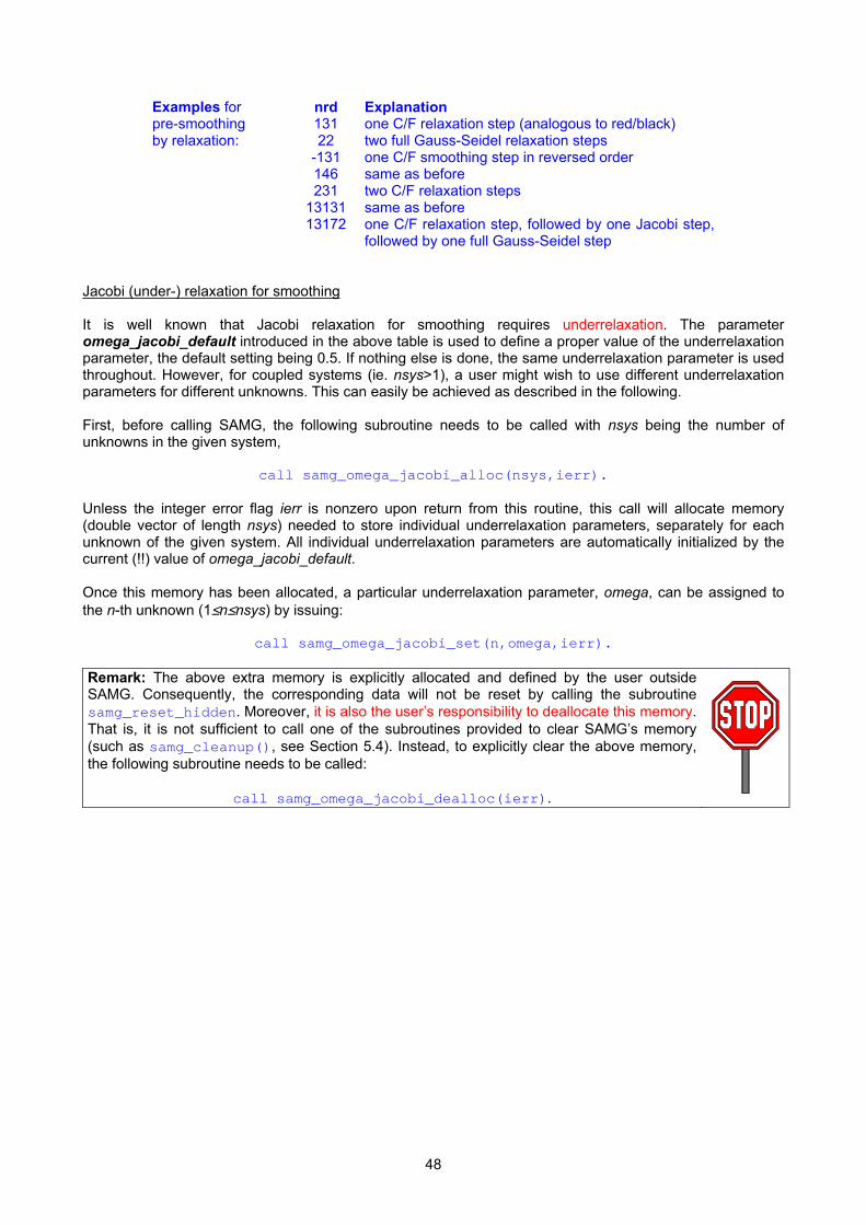
48

nrd Explanation 131 one C/F relaxation step (analogous to red/black) 22 two full Gauss-Seidel relaxation steps

-131 one C/F smoothing step in reversed order 146 same as before 231 two C/F relaxation steps

13131 same as before

Examples for pre-smoothing by relaxation:

13172 one C/F relaxation step, followed by one Jacobi step, followed by one full Gauss-Seidel step

Jacobi (under-) relaxation for smoothing It is well known that Jacobi relaxation for smoothing requires underrelaxation. The parameter omega_jacobi_default introduced in the above table is used to define a proper value of the underrelaxation parameter, the default setting being 0.5. If nothing else is done, the same underrelaxation parameter is used throughout. However, for coupled systems (ie. nsys>1), a user might wish to use different underrelaxation parameters for different unknowns. This can easily be achieved as described in the following. First, before calling SAMG, the following subroutine needs to be called with nsys being the number of unknowns in the given system,

call samg_omega_jacobi_alloc(nsys,ierr). Unless the integer error flag ierr is nonzero upon return from this routine, this call will allocate memory (double vector of length nsys) needed to store individual underrelaxation parameters, separately for each unknown of the given system. All individual underrelaxation parameters are automatically initialized by the current (!!) value of omega_jacobi_default. Once this memory has been allocated, a particular underrelaxation parameter, omega, can be assigned to the n-th unknown (1≤n≤nsys) by issuing:

call samg_omega_jacobi_set(n,omega,ierr). Remark: The above extra memory is explicitly allocated and defined by the user outside SAMG. Consequently, the corresponding data will not be reset by calling the subroutine samg_reset_hidden. Moreover, it is also the user�s responsibility to deallocate this memory. That is, it is not sufficient to call one of the subroutines provided to clear SAMG�s memory (such as samg_cleanup(), see Section 5.4). Instead, to explicitly clear the above memory, the following subroutine needs to be called:

call samg_omega_jacobi_dealloc(ierr).

49

7.2.2 The coarsest-level solver Various solvers for the coarsest-level equations are included in SAMG. The standard and most robust way to solve the coarsest-level equations is by a direct solver. Clearly, the coarsest level then should not be too fine: First, the process of solving the coarsest-level equations should not be more expensive than the smoothing process on the finest level, say. Second, the memory requirement of the direct solver should remain acceptable. Generally, a few hundred variables on the coarsest level (cf. parameter nptmn in Section 7.1.5) should be quite acceptable in that respect. Remark: It is not necessary to solve the coarsest-level equations accurately, an accuracy of 1-2 digits is sufficient. Consequently, rather than using a direct solver, one might be attempted to use an iterative solver. This would have the advantage of a lower memory requirement which, in turn, would allow for much finer coarsest levels. However, in complex applications, the convergence behavior of iterative solvers may turn out to be fairly unpredictable, causing iterative solvers to become less favorable. Parameter Explanation Default

Solvers available for the coarsest-level equations Specifies coarsest-level solver. If nrc=0, a default solver is selected, see below.

Type of solver 1 Iterative application of currently selected smoother 2 ILU(0) preconditioned CG 3 ILUT preconditioned BiCGstab 4 Diagonally preconditioned CG 5 Diagonally preconditioned BiCGstab 6 Full Gauss elimination 7 Sparse Gauss elimination 8 Least squares solver (robust but very expensive!)

[1:1],

nrc_typ

9 User-supplied solver (see Section 9.2.1) The remaining digits are relevant only for the iterative solvers, nrc_typ=1-5. If these digits are not specified (or if they are zero), default settings will be used for the corresponding parameters, see below.

[2:2], lfil_cl Fill-in parameter to be used in case of ILUT. (Regarding the droptol parameter, see droptol_cl further below.)

[3:4], conv_stop

The iteration will terminate if the residual has been reduced by conv_stop := digit4*10**(-digit3).

nrc

[5: ], itmax_conv

The coarsest-level iteration will be terminated after (at most) itmax_conv iterations. A warning will be issued if the finally achieved residual reduction is worse than sqrt(conv_stop).

0

Default values relevant for the coarsest-level solver nrc_default Solver to be used if nrc=0 on input. 7

lfil_cl_default ILUT fill-in parameter to be used if lfil_cl is not specified or zero. 9

conv_stop_default Residual reduction required for termination of iterative solvers if conv_stop is not specified or zero. 0.1d-1

itmax_conv_default Maximum number of iterations allowed for iterative solvers if itmax_conv is not specified or zero. 200

Remark: If - according to the setting of the parameter isym - the given problem is not symmetric, the CG solvers (nrc_typ=2 and =4) will automatically be replaced by the corresponding ones using BiCGstab (nrc_typ=3 and =5). Remark: The least squares solver (nrc=8) is only for test purposes, it is very expensive! On the other hand, it provides the most robust way to solve the coarsest-level equations, in particular, in case of singular or nearly singular matrices.

50

Examples: nrc Explanation

0 Sparse Gauss elimination. 4 At most 200 iteration steps are performed to reach a residual reduction on the

coarsest level by 0.01. Method: Diagonally preconditioned CG (unless the matrix is non-symmetric, in which case diagonally preconditioned BiCGstab will be used instead).

2723812 At most 812 iteration steps are performed to reach a residual reduction on the coarsest level by 0.03. Method: ILU(0) preconditioned CG (unless the matrix is non-symmetric, in which case BiCGstab with ILUT(7) pre-conditioning will be used instead).

300020 At most 20 iteration steps are performed to reach a residual reduction on the coarsest level by 0.01. Method: ILUT(9) preconditioned BiCGstab.

1011 At most 200 iteration steps are performed to reach a residual reduction on the coarsest level by 0.1. Method: Plain smoothing steps.

Parameter Explanation Default

Further parameters relevant for coarsest-level solver

nrc_emergency Number of the solver which is supposed to replace the one selected by nrc in the "emergency situation� that the number of variables on the coarsest level has become too large for some reason (ie, larger than nptmax). Only relevant if the setting of nrc corresponds to a direct solver. In this case, nrc_emergency should correspond to a reasonable iterative solver.

3

full_pivoting In case of full Gauss elimination: Logical to select full or partial pivoting. .false.

stability In case of sparse Gauss elimination: 0.0<stability<1.0. The smaller stability, the lower the fill-in, but also the stability (pivot-strategy!). The larger stability, the higher the fill-in, but also the stability.

0.25d0

iter_check In case of iterative application of the current smoother: Number of iterations to be performed before residuals are checked. 3

droptol_cl Threshold droptol if ILUT is used as preconditioner on the coarsest level. 0.5d-2

rcondx Control parameter for LSQ solution processes (needed to correctly detect the rank of a matrix). Remark: This parameter is relevant for all LSQ solution processes (not just for those which can be selected on the coarsest-level).

1.0d-6

51

7.3 Further parameters 7.3.1 Re-directing and limiting I/O By default, all print output is sent to the console. This can be changed by re-defining the hidden parameters logio and logfile accordingly. In addition to the primary parameters iout and idump, the hidden parameter mode_mess is used to control the amount of output.

Parameter Explanation Default Re-directing and limiting I/O

logio Integer. I/O unit for all print output. 6 logfile Character string. Name of logfile where to print output (empty string: console) � �

Integer. As described in Section 6.8, by setting the primary parameters iout and idump to something negative, all output regarding SAMG�s performance (setup, cycling history, etc) will be suppressed. However, general messages, warnings and error messages will still be printed unless the hidden parameter mode_mess is set accordingly:

1 All kinds of messages are printed. 0 Cntrl-messages18 are skipped. -1 In addition: General messages are skipped. -2 In addition: Warning messages are skipped.

mode_mess

-3 In addition: Error messages are skipped.

0

Consequently, to suppress all output, pass iout = -1 and idump = -1 to SAMG, and re-define the hidden parameter mode_mess by issuing call samg_set_mode_mess(-3). Remark: All output of SAMG is routed through a single routine, namely, samg_message. This routine is located in the file amguser.f and can be adjusted by the user to his needs19. For instance, output of SAMG may be transferred to a GUI. 7.3.2 Default values for various primary parameters The following table lists default values for some of the primary parameters.

Parameter Explanation Default Default values relevant for the solution approach

nsolve_default Default value to be used for nsolve if nsolve=0 on input 2 ncyc_default Default value to be used for ncyc if ncyc=0 on input 11030

ncgrad_default Default value to be used for ncgrad if ncgrad=0 on input 1 nkdim_default Default value (Krylov space) to be used for nkdim if nkdim=0 6

Default values in case of standard coarsening a_cmplx_default Default value to be used for a_cmplx if a_cmplx=0.0 on input. 2.5d0 g_cmplx_default Default value to be used for g_cmplx if g_cmplx=0.0 on input. 1.8d0 p_cmplx_default Default value to be used for p_cmplx if p_cmplx=0.0 on input. 1.8d0 w_avrge_default Default value to be used for w_avrge if w_avrge=0.0 on input. 2.5d0

Default values in case of aggressive coarsening a_cmplx_agg_default Default value to be used for a_cmplx if a_cmplx=0.0 on input. 1.2d0 g_cmplx_agg_default Default value to be used for g_cmplx if g_cmplx=0.0 on input. 1.2d0 p_cmplx_agg_default Default value to be used for p_cmplx if p_cmplx=0.0 on input. 1.2d0 w_avrge_agg_default Default value to be used for w_avrge if w_avrge=0.0 on input. 1.2d0

Default value for ioscratch

ioscratch_default I/O unit for scratch-files (eg. during memory management) used if the corresponding primary input value, ioscratch, is not specified or zero. 31

18 These are messages created by the automatic process described in Section 8.4. 19 If you need to adjust samg_message but have only a binary version of SAMG, please contact us, and we will make amguser.f available to you.

52

7.3.3 Some special parameters

Parameter Explanation Default Parameter influencing the performance

By default, the primary parameter res_in is only an output parameter. However, if the residual of the starting guess is already available before calling SAMG, you may want to tell SAMG to not recompute the residual but rather use the value which is passed via res_in. This can be done by setting ntake_res_in:

0 SAMG will regard res_in only as an output variable. That is, SAMG will compute the residual of the starting guess and return it via res_in.

ntake_res_in

1 SAMG will assume that, on input, res_in equals the residual of the starting guess. Be sure that this residual has been computed using the correct norm, namely, the one defined by norm_typ, see Section 6.6.4.

0

ncyc_min Minimum number of cycles to be enforced. 0

iter_pre

If AMG is used as a preconditioner, very rarely, it may happen that the accelerator runs into technical problems caused by the nature of the selected first approximation. In such cases, one can enforce SAMG to perform a few pre-iteration steps (ie, a few stand-alone cycles) before the accelerator is actually turned on. The number of pre-iteration steps (usually one or two) is defined by the setting of iter_pre. Remark: In the special case of a one-level method defined by igam>4 (see Section 8.5), one pre-iteration step corresponds to one step of plain Gauss-Seidel relaxation.

0

Parameter influencing only the output

ncyc_start To compute realistic values for the average residual reduction factor, the very first cycles should be ignored. (This is because residual reduction is generally faster in the very first cycles.) ncyc_start contains the number of cycles to be skipped. Only relevant for the print output.

2

show_un_res Integer: In addition to total residuals, display also individual residuals belonging to the unknowns with number 1,2,....., show_un_res. Only relevant for print output and only if nsys>1.

0

Parameter for debugging Defines the level of consistency checks during the execution phase.

0 No checking.

1

If nsys>1: In case of the unknown-based approach, check on all levels if all variables are still alive. In case of point-based approaches, additional checks are performed if check_order=.true. and/or check_allpnts=.true.

mode_debug

2 If nsys>1: The same as before except that the settings of check_order and check_allpnts are ignored.

1

check_order If nsys>1: Logical switch indicating whether or not it is to be checked that unknowns are ordered �consecutively� at each point. .false.

check_allpnts

If nsys>1: Logical switch indicating whether or not it is to be checked that all unknowns are living at all points. In addition, if nprim>0, it is checked that the primary unknown is living at all points. Attention: If this parameter is .false., the user has to explicitly set the two hidden logical parameters alluns_at_allpnts and nprim_at_allpnts.

.true.

53

7.3.4 Setting hidden parameters via the default switch n_default In Section 6.6.3, we have introduced several choices for the primary parameter n_default. The below tables display the values which are actually assigned to the hidden parameters nwt and ncg in these cases. n_default hidden parameters comments

Use if matrix A has no �critical� mixed-sign rows 10 nwt=1, ncg=1 11 nwt=1, ncg=12 12 nwt=1, ncg=11 13 nwt=1, ncg=111

Employs the simplest (direct) interpolation. Coarsening gets the more aggressive, the larger the 2nd digit of n_default. Note: Generally, aggressive coarsening reduces the memory requirements at the expense of a slower convergence.

15 nwt=2, ncg=1 16 nwt=2, ncg=12 17 nwt=2, ncg=11 18 nwt=2, ncg=111

Same as previous, except that standard interpolation is employed. In general, this kind of interpolation is more robust but also more costly.

Use if matrix A does have �critical�mixed-sign rows 20 or 99 nwt=2, ncg=4

21 nwt=2, ncg=42 22 nwt=2, ncg=41 23 nwt=2, ncg=411

Employs standard interpolation. Coarsening gets the more aggressive, the larger the 2nd digit of n_default. Note: Generally, aggressive coarsening reduces the memory requirements at the expense of a slower convergence.

25 nwt=3, ncg=4 26 nwt=3, ncg=42 27 nwt=3, ncg=41 28 nwt=3, ncg=411

Same as previous, except that extended standard interpolation is employed. In general, this kind of interpolation is more robust but also more costly.

The settings of the following table are completely analogous to those in the previous one, except that variables with only positive couplings are treated �by absolute value�. Hence, the settings in the following table ensure that - formally - coarsening does not get stuck in case there are many rows with only positive couplings. Since this happens occasionally, the values of the next table are generally preferable over the previous ones. n_default hidden parameters comments

Use if matrix A has no �critical� mixed-sign rows 30 nwt=1, ncg=2 31 nwt=1, ncg=22 32 nwt=1, ncg=21 33 nwt=1, ncg=211 35 nwt=2, ncg=2 36 nwt=2, ncg=22 37 nwt=2, ncg=21 38 nwt=2, ncg=211

Settings 30-38 are analogous to the settings 10-18, respectively, except that variables with only positive couplings are treated �by absolute value�.

Use if matrix A does have �critical� mixed sign rows 40 or 0 nwt=2, ncg=5

41 nwt=2, ncg=52 42 nwt=2, ncg=51 43 nwt=2, ncg=511 45 nwt=3, ncg=5 46 nwt=3, ncg=52 47 nwt=3, ncg=51 48 nwt=3, ncg=511

Settings 40-48 are analogous to the settings 20-28, respectively, except that variables with only positive couplings are treated �by absolute value�. n_default=40 and n_default=42 are recommended as reasonable settings in case of standard and aggressive coarsening, respectively. Note that n_default=0 corresponds to n_default=40.

Remark: Defining a hidden parameter by its set-routine (see Section 5.3) has a higher priority than selecting it via n_default. That is, explicit definitions overwrite values defined via the setting of n_default. Moreover, explicitly defined parameters keep their value until they are either explicitly re-defined or cleared. Consequently, re-calling SAMG with a new value of n_default has no effect on the value of any explicitly defined hidden parameter.

54

8 Special Options in Using SAMG This section describes various special SAMG features. Some of them - such as the automated reuse of SAMG's setup phase in Section 8.4.2 - are still under development and optimization. However first versions are released for testing. Unless explicitly stated otherwise, all hidden parameters introduced in this section can be accessed as described in Section 5.3. 8.1 OpenMP parallelization Depending on the type of license purchased, SAMG is OpenMP parallelized20. If the library has been built with proper compiler and linker flags, most multi-processor machines will automatically make use of the OpenMP feature and choose the number of threads to be used as either p or p-1 where p denotes the number of processors of that machine. If more than 1 thread is employed, SAMG will report the exact number of threads (assuming the value of mode_mess has been set to 1, see Section 7.3.1) as in the following example: >>> CNTRL: ------------------------------------------------------------------ >>> CNTRL: Calling main control mechanism of SAMG ..... Call # 1 >>> CNTRL: ------------------------------------------------------------------ >>> MESSG: Current number of threads = 2 >>> CNTRL: ------------------------------------------------------------------ If the number of threads is to be defined explicitly, one can, for instance, set the environment variable OMP_NUM_THREADS prior to starting the application from the console,

setenv OMP_NUM_THREADS <number of threads>. Alternatively, the requested number of threads can be defined by calling standard OpenMP routines inside an application. 1. Generally, the number of threads should be less than or equal to the number of

processors of the machine given. For some machines (in particular, for some SGI�s), one should even assure that the number of threads is strictly less than the number of processors. Otherwise, performance may substantially degrade.

2. SAMG does not change the number of threads. 3. SAMG is not thread-safe! That is, SAMG may be called only by one thread at a time.

Regarding an optimal OpenMP performance, there are a few new parameters. All of them are initialized to reasonable default values and, if required, can be changed as described in Section 5.3. However, under all normal conditions, there should be no need to change the default values.

20 Currently, only the most expensive components of SAMG�s solution phase have been OpenMP parallelized. Parallelization of the setup phase is under development.

55

Parameter Explanation Default

Parameters relevant for fine-tuning the OpenMP performance Integer switch to select between different variants to perform the fine-to-coarse residual restriction in parallel. Generally, a higher parallel efficiency requires additional memory. Although the difference in parallel efficiency - measured just for the residual restriction itself - may be substantial (e.g., around 10% between variant -1 and 1), its effect on the global performance is only marginal. Hence the additional memory required for a higher efficiency typically will not pay, and option 1 is a good default value.

-1

The transposed interpolation matrix (used for restricting the residual) is computed at the beginning of the solution phase and then kept in memory, resulting in highest parallel efficiency at the expense of quite some extra memory.

0 Sequential computation of residual restriction, no OpenMP.

1 Residual computation is parallel. However, the restriction of the residual (via the transposed interpolation matrix) is sequential. Parallel efficiency is reasonable, no additional memory required.

2

Residual computation is parallel. The restriction of the residual is also parallel, based on OpenMP REDUCTION operations for vectors. However, this is not supported by all compilers. In addition, there is a risk of stack overflows.

irestriction_openmp

3 Similar as 2, except that memory is explicitly allocated (size: number of variables times number of threads). The risk of stack overflows is avoided.

1

nmin_matrix Minimum number of rows per thread in matrix times vector operations required for SAMG to really run in parallel. 40,000

nmin_vector Minimum number of rows per thread in vector - vector operations required for SAMG to really run in parallel. 100,000

nmin_matrix_resc Min. number of rows per thread in transposed matrix times vector operations for computing the restriction required for SAMG to really run in parallel.

100,000

8.2 Stopping criteria for the iterative solution process Besides robust convergence, the availability of reasonable and reliable stopping criteria is of major concern for iterative solvers. Two standard criteria have already been introduced earlier, controled by the primary parameters ncycle (maximum number of iterations, Section 6.5) and eps (prescribed residual reduction, Section 6.2). Although these two stopping criteria are sufficient for many situations, in general, additional criteria are needed. Corresponding developments are still ongoing, but some important stopping criteria are already available. Note that the selection of reasonable stopping criteria depends on the concrete situation and should be done with care. The currently available criteria (including the above-mentioned standard ones), can be subdivided into the following two classes which will be described separately in the following sections.

Convergence criteria Criteria which aim at detecting whether the current approximation satisfies a user-prescribed accuracy.

Safety checks Checks which aim at detecting whether, for any reason (such as roundoff or divergence), it just makes no sense any more, to continue the iteration process.

Remark: Except for the standard criteria controled by ncycle and eps, all of the following criteria are effective only in the default situation that AMG is used as a preconditioner for either CG, BiCGstab or GMRES. That is, if accelerators are explicitly de-activated by the user (so that AMG operates as a stand-alone solver), all of the new parameters introduced below are ignored.

56

8.2.1 Convergence criteria Two criteria are currently available to detect whether the most recent iteration ui, say, satisfies a user-prescribed accuracy, one based on the residual ( || ||i ires f Au= − ) and one on the approximation itself:

The residual criterion, controled by the primary parameter eps, has already been introduced in Section 6.2 but is repeated here for completeness. ires and 0res denote the residuals of the i-th and the 0-th iteration step21, respectively, measured in the norm as selected by the primary parameter norm_typ (default = L2-norm, see Section 6.6.4). eps≥0.0d0 The residual criterion requires 0ires eps res≤ ⋅ to be fulfilled.

Residual criterion

eps<0.0d0

The residual criterion requires | |ires eps≤ to be fulfilled. Note: Compared to the previous "relative" criterion, this "absolute" one should be used when a fixed residual reduction does not make sense, for instance, in time stepping applications. There, eps is typically of the form || ||eps fη= − with η being a reasonably small number and || ||f the norm22 of the current right hand side.

Approximation

criterion

This criterion requires 1 max max 1 max|| || max(|| || ,|| || )i i i iu u factor_app_var u u− −− < ⋅ to be fulfilled with a reasonably small value of the hidden parameter factor_app_var (see below). Note: This criterion is only meaningful if the iteration converges sufficiently fast. Otherwise, it may be fulfilled although the current approximation is still far from the wanted solution, for instance, if convergence is extremely slow.

Both of the above criteria can be selected and de-selected via the hidden integer parameter icrits. This parameter, as well as the threshold parameter factor_app_var, can be accessed and modified in the usual way as described in Section 5.3.

Parameter Explanation Default Parameters related to the convergence criteria

Hidden integer parameter. If icrits=0, all convergence criteria are de-selected (not recommended!). Otherwise, the first digit specifies how the selected criteria are to be interpreted. The remaining digits are used to select/de-select each single criterion individually.

1 Iteration of SAMG stops only if all of the selected convergence criteria are fulfilled.

[1:1]

2 Iteration of SAMG stops if just one of the selected convergence criteria is fulfilled.

0 The residual criterion is de-selected. [2:2] 1 The residual criterion is selected. 0 The approximation criterion is de-selected.

icrits

[3:3] 1 The approximation criterion is selected.

110

factor_app_var Hidden parameter defining the approximation criterion, see above. 1.0d-10

21 By the 0-th iteration step we mean the starting guess. 22 This norm should be the same as the one which is used to measure the residuals. Note that ||f|| then coincides with res0 if the starting guess is the zero vector.

57

8.2.2 Safety checks The most straightforward safety check is to simply restrict the total number of allowed iteration steps. As already described in Section 6.5, this can be achieved by setting the primary (sub-) parameter ncycle to the maximum number of allowed steps. Additional safety checks and related parameters are described in the following.

Quasi residual

check

At each23 iteration step, this check compares the quasi residual (implicitly computed as part of the currently selected accelerator) and the real residual (that is, || ||f Au− , computed "from scratch"). Theoretically, both residuals should be identical. In practice, however, during the process of a convergent iteration, roundoff influence will cause these residuals to become increasingly different up to the point, where both residuals are different in all digits. At that point, it generally does not make much sense to continue iterating: Although the quasi residual may still decrease further in subsequent iteration steps, there is no corresponding increase of accuracy any more and everything is dominated by roundoff error. This can be seen by looking at the real residual which does not decrease any further. This different behavior gives rise to a very convenient safety check to detect whether the level of roundoff has been reached and iteration should be stopped. This is based on the value max( , ) / min( , )q qratio res res res res= where qres and res denote the quasi and real residuals, respectively, of a given iteration. Obviously, if this ratio is larger than 10, say, the two residuals should be completely different. The final check is now as follows: Given a (small) number n>0, the quasi residual check limits the number of iterations for which ratio factor_quasi_res> is allowed to n. If the number of such iterations exceeds n, SAMG will stop iterating and return with a warning. Depending on whether the currently active accelerator is CG, BiCGstab or GMRES, the warning code will be -831, -841 and -851, respectively. The concrete value of the hidden threshold parameter factor_quasi_res (see below) should be around 10.0 or larger.

Residual stagnation

check

Given a (small) number n>0, this check controls the variation of the (real) residuals over the last n+1 iterations24. If max min/ _res res factor_res var< , SAMG will stop iterating and return with a warning. Depending on whether the currently active accelerator is CG, BiCGstab or GMRES, the warning code will be -832, -842 and -852, respectively. The hidden parameter factor_res_var (see below), should be (slightly) larger than 1.0. (Note that a value ≤1.0 would cause the above inequality to be never fulfilled, meaning that the stagnation check is actually de-activated.)

Limiting accelerator

re-starts

Given a number n>0, this check limits the number of accelerator re-starts25 to n. If this number is exceeded, SAMG will stop iterating and return with a warning. Depending on whether the currently active accelerator is CG, BiCGstab or GMRES, the warning code will be -833, -843 and -853, respectively.

23 The hidden parameter nth_res_scratch (see below), can be used to skip some steps to reduce the numerical work. 24 minres and maxres denote the minimum and maximum values of the residuals, taken over the last n iterations. 25 For safety reasons, all accelerators are automatically re-started in case of unexpected numerical troubles.

58

All safety checks can be selected and de-selected via the hidden integer parameter iauto_stop. This parameter, as well as the other hidden parameters contained in the following table, can be accessed and modified in the usual way as described in Section 5.3.

Parameter Explanation Default Parameters related to the safety checks

If iauto_stop=0, all safety checks are de-selected. Otherwise, its digits are used to select/de-select individual safety checks. Regarding the meaning of n in this table, see the above detailed description of the safety checks.

[1:1], iauto_stop_level

Currently, the concrete value of the 1st digit has no meaning. Just set it to 1. 0 Quasi residual check is de-selected. [2:2],

icheck_quasi_res n Quasi residual check is selected.26 0 Residual stagnation check is de-selected. [3:4],

num_old_res n Residual stagnation check is selected.26 [5:6],

num_old_apps Reserved for solution stagnation check. Not yet implemented. 0 Accelerator re-starts are not limited.

iauto_stop

[7:7], nfailed_accsteps n Maximum number of acceleration re-

starts.26 Currently only for BiCGstab!

1103003

factor_quasi_res Factor used for the quasi residual check as described before. See also the below parameter nth_res_scratch. 1.0d1

factor_res_var Factor used for the residual stagnation check as described before. 1.01d0 This parameter has been introduced to reduce the number of residuals which are computed "from scratch" (that is, the "real" residuals) in performing the quasi residual check.

=0 Each residual is computed from scratch (default).

=n>0 Only every n-th residual is computed from scratch. This should be used only for "well-behaved" problems for which comparisons of the quasi and the real residual are not necessary at every iteration of SAMG.

nth_res_scratch

=n<0 Not yet implemented.

0

26 Regarding the meaning of n, see the detailed description of the safety checks in the previous table.

59

8.3 Forcing special variables into coarse or fine levels Depending on the application at hand, a user may wish to force particular variables to exist on all coarse levels or to strictly remain only on the finest level. This can easily be achieved as described in the following. First, before calling SAMG, the following subroutine needs to be called with nnu being the total number of variables in the given system,

call samg_cvec_alloc (nnu,ierr). Unless the integer error flag ierr is nonzero upon return from this routine, this call will allocate memory (integer vector of length nnu) needed to mark those variables which the user wants to be treated specially.27 Once this extra memory has been allocated, any variable i with 1 ≤ i ≤ nnu can be marked by assigning an integer �priority value� ipriority as follows:

call samg_cvec_set(i,ipriority,ierr). Legal values are ipriority = -5, -4,...., 1, 2 where ipriority=0 means that no special condition is imposed, that is, the control over i is completely left to SAMG (the default). Remark: Since the above extra memory is explicitly allocated by the user outside SAMG, it is also the user�s responsibility to deallocate this memory. That is, it is not sufficient to call one of the subroutines provided to clear SAMG�s memory (such as samg_cleanup(), see Section 5.4). Instead, to explicitly clear the above memory, the following subroutine needs to be called: call samg_cvec_dealloc(ierr).

8.3.1 Explicitly forcing variables to exist on all coarse levels In order to force the i-th variable to exist on all coarse levels, samg_cvec_set needs to be called with ipriority=1 or =2. In detail:

Parameter Explanation Forcing variables to exist on all coarser levels

0

Nothing is enforced on the i-th variable, that is, control over i is completely left to SAMG. Calling samg_cvec_set with i and ipriority=0 is equivalent to not calling it for i at all. The setting ipriority=0 is needed only if, for some technical reason, the priority status of some i is to be re-set explicitly.

1 i is forced to exist on all coarse levels unless SAMG detects that, for some important reason, this may not be a good idea.

ipriority

2 i is definitely forced to exist on all coarse levels. Warning: If a user decides to force special variables to exist on all coarse levels, he should know what he is doing. Generally, the number of corresponding variables should be relatively low and carefully selected. Otherwise, memory requirements may drastically increase! Remark: For point-based approaches forcing into coarse levels should be �pointwise�. That is, if a variable is forced into all coarser levels, all variables living at the same point should also be forced into all coarse levels by assigning the same ipriority value to all these variables.

27 Note that, if the user forces certain variables into all coarser levels (ie, if ipriority=1, 2, -4 or -5) , the vector allocated via the subroutine samg_cvec_alloc will be extended internally to SAMG. This is done automatically, and the user does not need to care. However, the user can avoid this memory extension by allocating more memory from the beginning. For instance, by callig samg_cvec_alloc with 2*nnu rather than nnu.

60

8.3.2 Explicitly forcing variables to remain only on the finest level In order to force the i-th variable to strictly remain only on the finest level, samg_cvec_set needs to be called with ipriority=-1 or =-2. Variables marked in this way will not be included in the AMG solution process, that is, they will not be involved in the hierarchy of levels and they will not be corrected from coarser levels. In this sense, their numerical treatment is completely decoupled from that of the rest of the linear system. Consequently, variables of that type need to be included in the overall solution process by other means: While variables marked by ipriority=-1 are included as part of the finest level smoothing process, variables marked by ipriority=-2 are simultaneously treated by some block solver instead. The latter provides the basis for defining some kind of �alternating Schwarz process� as described next. In detail, the following settings are possible:

Parameter Explanation Forcing exceptional variables to exist on the finest level only The setting ipriority=-1 to mark a set of �exceptional variables� is supposed to be used for relatively simple situations for which the smoother works sufficiently well for resolving these exceptional variables:

-1 i is forced to strictly remain only on the finest level, completely decoupled from the overall AMG process. However, such variables are still included in the finest-level smoothing process.

In more complex situations, a user may wish to solve a set of exceptional variables simultaneously by some kind of block solver. This is achieved by marking these variables by ipriority = -2:

-2

i is forced to strictly remain only on the finest level, completely decoupled from the overall AMG process. Instead, such variables will be solved for simultaneously by a block solver. Remark: If smoothing is done by Gauss-Seidel relaxation, these variables are skipped in the finest level smoothing process. Otherwise, they are included.

In addition, settings ipriority = -3, -4 and -5 are allowed: All variables marked this way are solved for simultaneously and together with those marked by ipriority = -2. However, in contrast to the latter, variables marked by ipriority = -3, -4 or -5 are included in the hierarchical process. More precisely, they are included in exactly the same way as variables which are marked by ipriority = 0, =1 and =2, respectively:

-3 Nothing is enforced on the i-th variable, that is, control over i is completely left to SAMG (cf. ipriority=0).

-4 i is forced to exist on all coarse levels unless SAMG detects that, for some important reason, this may not be a good idea (cf. ipriority=1).

ipriority

-5 i is definitely forced to exist on all coarse levels (cf. ipriority=2). Although, in principle, the settings -2,....,-5 can be assigned to variables in an arbitrary way, the usual way to apply these settings is to first define a subset of exceptional variables by assigning ipriority=-2 (�Schwarz subset�) and then use ipriority=-3, -4 and -5 to specify a reasonable overlap (�Schwarz overlap�). In this context, see also the hidden parameter nblk_overlap below which can be used to automatically include overlap variables in the block solve.

61

The following hidden parameters are available to specify details of the �alternating Schwarz process�, with or without overlap:

Parameter Explanation DefaultParameters relevant for the �Schwarz process�

Integer parameter specifying when to perform a Schwarz block solution step simultaneously for all variables marked by ipriority = -5,....,-2.

0 Skip block solution completely (for debugging only!) 1 Block solution after each cycle 2 Block solution after each (full) smoothing step

nblk_solve

3 Block solution after each (partial) smoothing step

1

Integer parameter to select the type of block solver used. 1 Full Gauss elimination with partial pivoting 2 Full Gauss elimination with total pivoting

nblk_solver

3 Sparse Gauss elimination 3

Integer parameter specifying the width of �overlap� between the Schwarz subset (as defined by the setting ipriority = -2) and the remainder of the variables. This parameter can be used to automatically select and add overlap variables to the block of variables to be solved for simultaneously. This can be done instead of or in addition to marking variables by manually assigning ipriority = -3, -4 or -5 to individual variables as described further above. Warning: Automatically adding overlap variables is very convenient. However, depending on the overall connectivity structure of the variables, a vast number of additional variables might be introduced. Use this option with care!

0 No overlap

1 Overlap 1: Add all direct neighbors of variables marked by ipriority = -2 (unless they have already been marked manually)

nblk_overlap

2 Overlap 2: analogously

0

nblk_max

Integer parameter specifying maximum number of exceptional variables to be solved for simultaneously. If this number is exceeded, SAMG will terminate with error (error code 260). Warning: Practical values depend on the block solver selected. For the current SAMG release, block solution is done by a direct solver. Consequently, the number of variables to be solved for simultaneously should not be too large. Roughly, for the full and the sparse Gauss elimination, that number should not exceed 500 and 2000, respectively.

1000

The following parameters are very special Integer parameter to be used only for debugging

0 Standard residual computation

nblk_resid 1 Skip variables marked by ipriority = -2 in computing residuals 0

Integer parameter for initializing some debug information 0 No debug mode

nblk_debug

1 Compute and display residuals of Schwarz block systems. 0

blk_stab

Double parameter, only needed for sparse Gauss elimination. Its value has to be between 0.0 and 1.0: the smaller this parameter, the lower the fill-in, but also the stability (pivoting-strategy!) and the higher this parameter, the higher the fill-in, but also the stability.

0.25d0

blk_fillexp

Double parameter, only needed for sparse Gauss elimination. The smaller this parameter, the lower the memory allocation and the larger this value, the higher the memory allocation. Usually, its value should be around 0.5.

0.5d0

Remark: For point-based approaches forcing into the finest level should be �pointwise�. That is, if a variable is forced to strictly remain only on the finest level, the same should be true for all variables living at the same point by assigning the same ipriority value to all these variables.

62

8.3.3 Additional features As an alternative to setting ipriority values via calling the subroutine samg_cvec_set, one may pass a list of ipriority values for all variables to SAMG via a file. In addition, there are some auxiliary hidden parameters which can be used to force particular variables into the coarse levels, or to leave them on the finest one. This is for simplification in selected frequent situations.

Parameter Explanation Standard Specifying a list of ipriority values via a file

cset_read Character string. If not empty, cset_read denotes the name of a (formatted) file where a list of ipriority values is found, one entry per row. " "

Auxiliary parameters for frequent situations

cset_zerodiag Integer: Used to force all variables, the corresponding matrix rows of which have a zero diagonal entry, either into all coarse levels, or to force them to remain on the finest level. Legal values are -5,....,2. Example: Setting cset_zerodiag=-1 forces all such variables to remain only in the finest level.

0

cset_lessvars

Integer: Used to force all points which have less than nsys variables attached, into the coarse levels or to remain on the finest level. Legal values are -5,....,2. Example: Setting cset_lessvars=2 forces all such points into the coarse levels.

0

cset_lastpnt

Integer: Used to force the last finest-level point into the coarse levels or to force it to remain on the finest level. Legal values are -5,....,2. Example: Setting cset_lastpnt=1 forces all variables attached to the last point into the coarse levels, unless SAMG decides that this is not a good idea.

0

Integer: Used to force variables corresponding to particularly long rows into the coarse levels or to force them to remain on the finest level. Legal values are -5,....,2. Example: Setting cset_longrow=-1100 forces all variables to remain on the finest level which correspond to rows with 100 entries or more.

[1:1]

ipriority value to be assigned to all variables which relate to rows which have a lenghth greater than or equal to the integer threshold defined by the remaining digits (see next). Note: a negative sign of cset_longrow will be attached to ipriority. This way, all legal values of ipriority can be defined.

cset_longrow

[2: ] Defines the "critical" row length (see before).

0

The above options/parameters to set ipriority values can be used simultaneously. In this case, we have the following priority sequence in decreasing order,

cset_read → cset_lessvars → cset_lastpnt → cset_longrow → cset_zerodiag. If the above options/parameters are used, the subroutine samg_cvec_alloc does not need to be called, memory will be allocated automatically.

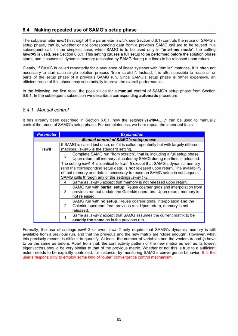
63

8.4 Making repeated use of SAMG�s setup phase The subparameter iswit (first digit of the parameter iswtch, see Section 6.6.1) controls the reuse of SAMG�s setup phase, that is, whether or not corresponding data from a previous SAMG call are to be reused in a subsequent call. In the simplest case, when SAMG is to be used only in �one-time mode�, the setting iswit=5 is used, see Section 6.6.1. This setting causes a full setup to be performed before the solution phase starts, and it causes all dynamic memory (allocated by SAMG during run time) to be released upon return. Clearly, if SAMG is called repeatedly for a sequence of linear systems with �similar� matrices, it is often not necessary to start each single solution process �from scratch�. Instead, it is often possible to reuse all or parts of the setup phase of a previous SAMG run. Since SAMG�s setup phase is rather expensive, an efficient reuse of this phase may substantially improve the overall performance. In the following, we first recall the possibilities for a manual control of SAMG�s setup phase from Section 6.6.1. In the subsequent subsection we describe a corresponding automatic procedure. 8.4.1 Manual control It has already been described in Section 6.6.1, how the settings iswit=4,�,1 can be used to manually control the reuse of SAMG�s setup phase. For completeness, we here repeat the important facts:

Parameter Explanation Manual control of SAMG�s setup phase

If SAMG is called just once, or if it is called repeatedly but with largely different matrices, iswit=5 is the standard setting.

5 Complete SAMG run �from scratch�, that is, including a full setup phase. Upon return, all memory allocated by SAMG during run time is released.

The setting iswit=4 is identical to iswit=5 except that SAMG�s dynamic memory (and the corresponding setup data) is not released upon return. The availability of that memory and data is necessary to reuse an SAMG setup in subsequent SAMG calls through any of the settings iswit=1-3.

4 Same as iswit=5 except that memory is not released upon return.

3 SAMG run with partial setup: Reuse coarser grids and interpolation from previous run but update the Galerkin operators. Upon return, memory is not released.

2 SAMG run with no setup: Reuse coarser grids, interpolation and the Galerkin operators from previous run. Upon return, memory is not released.

iswit

1 Same as iswit=2 except that SAMG assumes the current matrix to be exactly the same as in the previous run.

Formally, the use of settings iswit=3 or even iswit=2 only require that SAMG�s dynamic memory is still available from a previous run, and that the previous and the new matrix are �close enough�. However, what this precisely means, is difficult to quantify. At least, the number of variables and the vectors iu and ip have to be the same as before. Apart from that, the connectivity pattern of the new matrix as well as its lowest eigenvectors should be very similar to that of the previous matrix. Whether or not this is true to a sufficient extent needs to be explicitly controlled, for instance, by monitoring SAMG�s convergence behavior. It is the user�s responsibility to employ some kind of �outer� convergence control mechanism.

64

8.4.2 Automatic control Remark: The automatic control mechanism described in this section is under development and its performance and reliability is subject to further optimizations. We would appreciate any information regarding practical experience as well as requests about improvements. The automatic control is activated by setting iswit>5. More precisely, the settings iswit=6,�,9 correspond to iswit=4,�,1 (in this order) with one important difference: While iswit=4,�,1 do not include any internal checks, the settings iswit=6,�,9 perform some automatic checks to find out whether or not the reuse of a previous setup makes sense. If not, SAMG automatically performes a new setup. Details are as follows:

Parameter Explanation Automatic control of SAMG�s setup phase

The settings iswit=6,�,9 correspond to iswit=4,�,1 (in this order) except that SAMG performs some automatic control mechanism.

6 Same as iswit=4.

7 Corresponds to iswit=3. More precisely, whenever possible and reasonable, SAMG runs with partial setup. Otherwise, SAMG makes a full fresh setup. Upon return, memory is not released.

8 Corresponds to iswit=2. More precisely, whenever possible and reasonable, SAMG runs with no setup. Otherwise, SAMG makes a full fresh setup. Upon return, memory is not released.

iswit

9 Same as iswit=8 except that SAMG assumes the current matrix to be exactly the same as in the previous run.

A typical situation for which SAMG�s automatic setup control mechanism has been developed is in solving time-dependent problems where system matrices often change only slowly from one time step to the next. In such cases, one may call SAMG with iswit=8 (or, more conservatively, with iswit=7). Whenever possible and reasonable, SAMG will then reuse the setup fully (or partially) from previous calls. More precisely, if no setup data is available (as, for instance, in the very first time step), SAMG will automatically make a full setup. In subsequent time steps, SAMG will then attempt to fully (or partially) reuse setups from previous time steps until this becomes less efficient than performing a new setup. (SAMG�s decision on what is more efficient - performing a new setup or reusing a previous one - is based on a few hidden parameters described further below.) Whenever SAMG�s automatic control mechanism is activated by setting iswit=8 or =7, between any two SAMG calls, the user may temporarily interrupt this automatic control by issuing

call samg_refresh(ierr) . This call releases all of SAMG�s dynamic memory, re-sets certain control data and forces SAMG to make a new setup next time it is called. A user should call this routine whenever he knows that the next linear system to be solved by SAMG will be substantially different from the previous one. This prevents SAMG from making (costly and) wasted attempts to reuse old data. Also, the refresh-routine should always be called whenever there is a conflict between the requirement to re-use setup data and the current parameter settings of SAMG, for instance, when the solution strategy (eg, the coarsening) is to be changed. Remark: If the automatic control is to be used, a detailed protocol about its history can be displayed. This is achieved by re-defining the hidden parameter mode_mess=1 (see Section 7.3.1). When may this automatic mechanism be used? In principle, the setting iswit=8 (or iswit=7) can be used if SAMG is applied repeatedly to any sequence of linear systems. However, one should observe that the automatic control mechanism involves some kind of �trial-and-error� process which may get rather expensive if the linear systems at hand are completely unrelated. In fact, using this mechanism might then get even more expensive than performing full setups each time SAMG is called (that is, calling SAMG with iswit=5).

65

When does this automatic mechanism pay? Clearly, the potential gain by reusing setup data is the higher, the smaller the typical number of iterations performed in SAMG�s solution phase. To be more specific, the cost of a full setup phase typically corresponds to that of 5-8 AMG cycles (ignoring accelerators such as conjugate gradient or BICG-STAB). Consequently, if the typical number of iterations performed in SAMG�s solution phase exceeds some 20-30, say, the potential benefit through employing the automatic control mechanism is fairly limited. Otherwise, it may be substantial. There are a few hidden parameters which specify details of how SAMG performs it's control mechanism.

Parameter Explanation DefaultParameters defining SAMG's automatic mechanism of reusing setup data

backup

Logical indicating whether or not the first guess should be saved upon entry to SAMG. This has to be .true. if SAMG - in case it needs to be "re-started" for any reason - should always start with the original first guess. Otherwise, SAMG might have to perform a re-start based on a different first approximation.

.true.

max_calls Maximum number of SAMG calls with no (or partial) setups before a full setup is enforced, independent of all other criteria. 4

Mode of setup control mechanism. The individual digits are as follows: [1:1],

max_cyc Number of cycles required before convergence is tested. This number should neither be too small nor too large.

[2:2], nstrict_ncyc

If nstrict_ncyc=0, SAMG regards it as a normal termination28 when the max number of cycles is reached. Otherwise not.

[3:3], nstrict_quasi

If nstrict_quasi=0, SAMG regards it as a normal termination28 when the quasi residual check is met. Otherwise not.

[4:4], nstrict_stagr

If nstrict_stagr=0, SAMG regards it as a normal termination28 when the residual stagnation check is met. Otherwise not.

[5:5], nstrict_stagu

If nstrict_stagu=0, SAMG regards it as a normal termination28 when the solution stagnation check is met. Otherwise not.

mode_cntrl

[6:6], ignore_warn

If ignore_warn=0, SAMG will temporarily interrupt the automatic control whenever SAMG reports a warning. Otherwise, warnings are simply ignored.

5

divergence

This parameter is only relevant if backup=.false., and if SAMG needs to be re-started because of divergence. In that case, if the average increase of the residual per iteration is greater than divergence, SAMG is re-started with the zero function. Otherwise, i.e. in case of �weak� divergence, SAMG uses the current approximation as first guess.

1.1d0

full_setup Cost of full setup in terms of number of cycles, ignoring accelerators (typically 6.0 or so). full_setup=0.0 means automatic selection based on internal time measurements.

0.0d0

partial_frac Fraction of partial and full setup cost (typically 0.3 or so). 0.3d0

rho_min Minimum convergence factor required for automatic control to be done. If not achieved, control will temporarily be deactivated. 0.9d0

rho_ok Convergence factor which shall be accepted without further attempt to optimize. 0.1d0 In contrast to what has been described in Section 5.3.3 regarding the modification of hidden parameters in general, the above hidden control parameters can be accessed via the special set- and get-routines called

samg_cntrl_set_ and samg_cntrl_get_ , respectively, followed by the name of the respective control parameter. For instance, to set the parameter rho_min to 0.75 and to avoid that the first approximation is saved, issue,

call samg_cntrl_set_rho_min(0.75d0) and call samg_cntrl_set_backup(0), respectively. Alternatively, the same can be achieved via the following two calls (restricted to Fortran users): call samg_setdble("rho_min",0.75d0) and call samg_setlogical("backup",.false.).

28 If SAMG terminates normally in this sense, potential warnings will be surpressed (ie, ierr=0 upon return). In case SAMG terminates abnormally in this sense, the automatic control is temporarily interrupted.

66

8.5 Special case: one-level methods SAMG�s cycling process is selected by the parameter ncyc described in Section 6.5. In particular, the sub-parameters igam and ncgrad define the type of cycle and the type of accelerator, respectively:

• ncgrad=0: accelerator defined by ncgrad_default (no accelerator if ncgrad_default=0), • ncgrad=1: CG, • ncgrad=2: BiCGstab, • ncgrad=3: GMRES (with Krylov dimension set by nkdim).

There are essentially two possibilities to use SAMG as a one-level method:

1. Select a multigrid cycle (igam=1), but set the maximum number of levels to 1, levelx=1. Then SAMG performs no coarsening (the whole setup phase will be skipped) but rather uses the currently selected smoother as an iterative solver. If ncgrad≠0 (or ncgrad=0 and ncgrad_default≠0), the smoother will be used as a preconditioner, otherwise stand-alone. Adjust nrd and nru to define details of the required smoothing steps (such as the number of smoothing sweeps per accelerator step), see Section 7.2.1.

2. Select igam>4. In this case, all multigrid-relevant parameter settings will be ignored and SAMG will execute one of several classical one-level-methods.29

The following table details all possibilities

igam Running SAMG in one-level mode Iterative application of smoother

If levelx>1, SAMG runs in multi-level mode. If levelx=1, no coarsening is performed, and the currently selected smoother (cf. Section 6.4.2 and 7.2.1) is used as an iterative solver30. If ncgrad≠0 (or ncgrad=0 and ncgrad_default≠0), the smoother is used as preconditioner for the respective accelerator, otherwise it is used stand-alone.

if nxtyp=0: Gauss-Seidel relaxation, variable-wise. if nxtyp=1: ILU(0) or MILU(0), depending on the hidden parameter milu. if nxtyp=2: ILUT31. if nxtyp=3: ILUTP31 or MILUTP31, depending on the hidden parameter milu. if nxtyp=5: For point-wise approaches: Block Gauss-Seidel relaxation.

igam=1

if nxtyp=6: For point-wise approaches: Block ILU. Classical one-level solvers (ignoring all multigrid-relevant parameters)29

igam=5 Diagonal preconditioning for the accelerator selected by ncgrad. ILU preconditioning for the accelerator selected by ncgrad. More precisely:

if ncgrad=1: ILU(0), independent of the value of igam.

if ncgrad=2: ILUT with fill-in parameter lfil=2*(igam-5)+1. The tolerance threshold droptol is a hidden parameter with default value 0.005.

igam=6-9

if ncgrad=3: same as for ncgrad=2. Remarks: • If CG is selected as an accelerator but the given matrix A is non-symmetric (according to the setting of

isym), CG is automatically replaced by BiCGstab (i.e. ncgrad=1 is replaced by ncgrad=2). • Sometimes it may be reasonable to perform a few pre-iteration steps (where one such step corre-

sponds to a single plain Gauss-Seidel relaxation step) before the respective accelerator is activated. By default, no pre-iterations are performed. This can be changed by means of the hidden parameter iter_pre described in Section 7.3.3.

29 This possibility to run SAMG in one-level mode is available for reasons of compatibility to earlier SAMG releases. However, we recommend to not use the setting igam>4 any more. Instead, use igam=1 and levelx=1. 30 The same is true if any of the stopping criteria for the coarsening process causes SAMG to not create any coarser levels, see Section 7.1.5. 31 Regarding the fill-in and droptol parameters, lfil_smo and droptol_smo, see Section 7.2.1.

67

8.6 Optimizing SAMG's performance (under construction) If applied in the standard way, SAMG does not know anything about geometry. Consequently, the �accuracy� of interpolation is necessarily limited. Nevertheless, for many applications, it is sufficiently good to ensure a rapid convergence which is essentially independent of the size of the given problem. In certain applications areas (eg, near-singular applications from linear elasticity), however, SAMG cannot ensure interpolation to be sufficiently accurate without knowing anything but the system matrix. Such �critical� applications are characterized by the fact that the first eigenvalues of A are extremely small and the corresponding eigenmodes are (smooth but) not constant. In linear elasticity, for instance, these modes correspond to the rigid body modes. In the context of SAMG, the main problem with such applications is that, in order to converge rapidly, the smoothest eigenmodes need to be interpolated with a sufficiently high accuracy, which actually has to be the higher the smaller the corresponding eigenvalue is. Consequently, unless the smoothest eigenmodes are essentially constant, special information is required to ensure a sufficiently good interpolation. One way to tackle such problems is by making the coordinates of grid points known to SAMG. This means that the black-box character of SAMG is lost to some extent. However, this information is usually available anyway, and - as long as no restrictions are put on the shape of the domain or the kind of grid to be used - the major advantages of SAMG still hold. Some of the more recent routines of SAMG attempt to exploit geometry in this way. The features outlined in this section are under development and not yet officially released. The external user should deactivate all related features by setting the main control parameter to zero, np_opt=0 (which is the default setting). 8.6.1 The main control parameter The parameter np_opt selects the level of optimization and passes some basic information on the origin of the problem at hand. Parameter Explanation Default

Optimization of interpolation Activates optimization of interpolation if np_opt ≠ 0.

[1:1], nopt Level of optimization: 1-9.

[2:2], ndim_space

Spatial dimension of the current problem (2 or 3). If ndim_space = 0, optimizations which require the knowledge of the dimension, will be skipped. Provides information on the current type of application

0 No particular information specified: Optimizations which require the knowledge of the application, will be skipped.

np_opt

[3: ], npclass

1 Linear elasticity (displacements only)

0

Remark: In order to take advantage of most of SAMG�s optimization routines, the user has to provide the subroutine samg_user_coo, described in Section 5.5, which defines the variable-to-coordinate mapping for the application at hand.

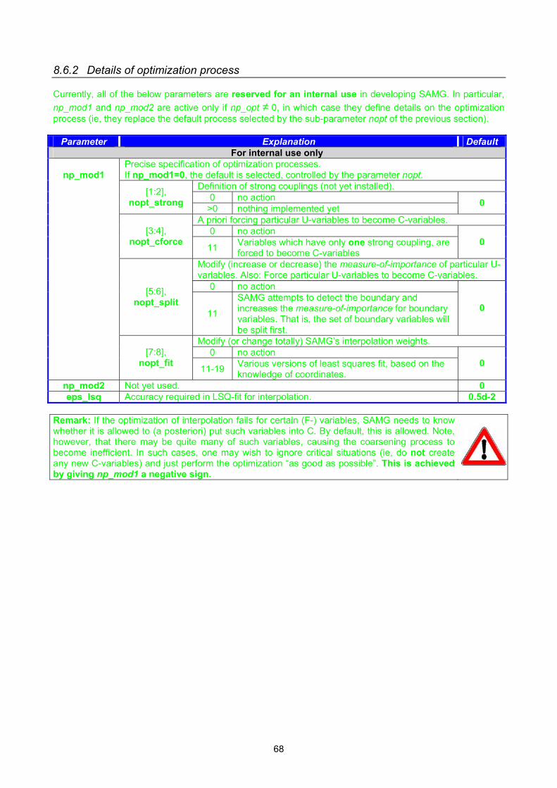
68

8.6.2 Details of optimization process Currently, all of the below parameters are reserved for an internal use in developing SAMG. In particular, np_mod1 and np_mod2 are active only if np_opt ≠ 0, in which case they define details on the optimization process (ie, they replace the default process selected by the sub-parameter nopt of the previous section).

Parameter Explanation Default For internal use only

Precise specification of optimization processes. If np_mod1=0, the default is selected, controlled by the parameter nopt.

Definition of strong couplings (not yet installed). 0 no action [1:2],

nopt_strong >0 nothing implemented yet 0

A priori forcing particular U-variables to become C-variables. 0 no action [3:4],

nopt_cforce 11 Variables which have only one strong coupling, are forced to become C-variables

0

Modify (increase or decrease) the measure-of-importance of particular U-variables. Also: Force particular U-variables to become C-variables.

0 no action [5:6], nopt_split

11

SAMG attempts to detect the boundary and increases the measure-of-importance for boundary variables. That is, the set of boundary variables will be split first.

0

Modify (or change totally) SAMG�s interpolation weights. 0 no action

np_mod1

[7:8], nopt_fit 11-19 Various versions of least squares fit, based on the

knowledge of coordinates. 0

np_mod2 Not yet used. 0 eps_lsq Accuracy required in LSQ-fit for interpolation. 0.5d-2

Remark: If the optimization of interpolation fails for certain (F-) variables, SAMG needs to know whether it is allowed to (a posteriori) put such variables into C. By default, this is allowed. Note, however, that there may be quite many of such variables, causing the coarsening process to become inefficient. In such cases, one may wish to ignore critical situations (ie, do not create any new C-variables) and just perform the optimization �as good as possible�. This is achieved by giving np_mod1 a negative sign.

69

8.7 Controling very specific output (involving files) This section describes features which control special file reading/writing activities of SAMG. These features are essentially reserved for debugging and not supposed to be used by an external user. The following hidden parameters are used in the subsequent sections:

Parameter Explanation Default Parameters for file reading/writing features

Character*1. Format of writing files. �f� Formatted writing. ioform �u� Unformatted writing.

�f�

filnam Root name of files which SAMG tries to find for reading. �temp� iodump I/O unit to be used if SAMG dumps matrices to disk. 32

filnam_dump Root name of files to be used for dumping matrices to disk. �level� iomovie I/O unit to be used if SAMG writes a sequence of iterations (�frames�) to a file. 34

ncframes Number of 1st frame to be written to file (up to the last one) -1 iogrid I/O unit to be used if SAMG writes grid info (coarsening pattern) to a file. 33

lastgrid Last grid for which coarsening pattern is to be written to a file. 0 8.7.1 Specifying file format Reading or writing can be formatted or unformatted. In case of reading (eg, Section 8.7.2), SAMG knows the format by looking into a special �format� file (suffix �.frm�). In case of writing (Sections 8.7.3-8.7.5), the hidden character*1 variable ioform defines the format SAMG is supposed to use. That is, issue either

call samg_setchar(’ioform’,’f’) or call samg_setchar(’ioform’,’u’), to specify whether writing is to be formatted or unformatted, respectively, the default being formatted. SAMG typically writes certain vectors of data to a file. This is done in the following way:

• if unformatted: write(io) (vec(i),i=1,nnu) • if formatted: do i=1,nnu; write(io,*) vec(i); enddo

8.7.2 Displaying error histories By default (assuming iout=2, see Section 6.8.2), SAMG displays the history of residuals from one iteration step to the next. For test purposes, it is sometimes instructive to additionally display the history of errors. This requires that the solution vector is known and contained in a file named �mysolution.sol�, say. (The file�s name is arbitrary but the special suffix �.sol� is obligatory!) This file can be either formatted or unformatted and has to be written as follows:

• if unformatted: write(io) (sol(i),i=1,nnu) • if formatted: do i=1,nnu; write(io,*) sol(i); enddo

In addition to the file �mysolution.sol�, there has to exist a formatted file �mysolution.frm� with just one line containing �u 4� or �f 4�, depending on whether �mysolution.sol� is unformatted or formatted, respectively32. To now make SAMG display histories of errors, just make the solution�s filename (hidden parameter filnam) known to SAMG by issuing the call

call samg_setchar(’filnam’,’mysolution’)

and give the parameter iswtch a negative sign.

32 The number �4� is used internally as a version control parameter.

70

Remarks: • If no solution filename is specified, the default name �temp� is assumed. • If the solution file does not exist, or if iout<2, no history of errors will be displayed. • SAMG will read the above files via the I/O unit ioscratch. • Error norms will be computed w.r.t. the norm selected by the parameter norm_typ. The special setting

norm_typ=3 corresponds to the energy norm. (If, according to the setting of parameter isym, the matrix A is not symmetric, the energy norm is automatically replaced by the L2-norm. )

8.7.3 Dumping matrices to disk The first digit of idump (see Section 6.8.3) can be used to direct SAMG to dump matrices to disk33, either formatted or unformatted, depending on the setting of ioform):

Parameter Explanation Dumping matrices to disk

1 Standard print output, no matrix dump. 2-6 Write matrices to disk: level 2 up to level idmp. 7 Write matrices to disk: level 2 up to the coarsest level. 8 Write finest-level matrix to disk (incl. right hand side).

idump

[1:1], idmp

9 Write all matrices to disk. If idmp>1, the matrices as described above are dumped to files using the root name filnam_dump, the default name being �level�. In addition, the level number will be added to the file�s root name. Files with the standard SAMG suffixes �.frm�, �.amg� and - in case of coupled systems - �.iu�, �.ip� will be created. In case of the finest level, the right hand side file (suffix �.rhs�) is created as well. Remarks: • If coordinates are available (via the user-supplied routine samg_user_coo), in addition a formatted file

with suffix '.coo' is created containing the list of coordinates. • In writing these files, the I/O unit iodump is used. 8.7.4 Writing intermediate approximations (frames) to disk In order to make SAMG write a sequence of iterations (�frames�) to a file, one after the other, starting with the k-th one (k≥0, where k=0 corresponds to the first guess) up to the final one, proceed as follows. The calling program has to open the file34 (formatted or unformatted, depending on the setting of ioform), linked to some I/O unit io, say. Then the hidden parameters ncframes (number of first iteration to be written) and iomovie (I/O unit used by SAMG for writing) have to be set:

call samg_setinteger(’ncframes’,k) and call samg_setinteger(’iomovie’,io). Remarks: • If ncframes is negative (the default), nothing will be written to disk. • The second call can be skipped, if io equals the default value of iomovie.

33 Regarding SAMG�s file format, see the corresponding separate SAMG document. 34 This cannot be done in case of shared libraries (suffix .DLL or .so,).

71

8.7.5 Writing coarsening pattern to disk For some given L ≥ 1, SAMG can write the coarsening pattern of levels 1,...,L to a file. More precisely, the coarsening pattern is a double (!) vector, color(1:nnu) say, defined as follows:

• color(i)=k: if k ≤ L is the highest level for which variable i is still "alive"; • color(i)=L+1: for all variables which are alive beyond level L.

In order to make SAMG write the vector color to a file, one has to proceed as follows: The calling program has to open the file34 (formatted or unformatted, depending on the setting of ioform), linked to some I/O unit io, say. Then the hidden parameters lastgrid (=L from above) and iogrid (I/O unit used by SAMG for writing) have to be set:

call samg_setinteger(’lastgrid’,L) and call samg_setinteger(’iogrid’,io).

Remarks: • If lastgrid is non-positive (the default), nothing will be written to disk. • The second call can be skipped, if io equals the default value of iogrid.

72

9 Special Interfaces 9.1 Alternative interfaces to call SAMG Usually, SAMG should be accessed via the standard interface described in Section 6. There are simplified interfaces which can be used instead, see Section 9.1.1. Another interface has been introduced in Section 9.1.2 in order to ensure some compatibility with the very first available AMG code which is still used today in various applications. However, unless one has good reasons, we generally do not recommend using these alternative interfaces any more. 9.1.1 Simplified interfaces (input via files) The following simplified interfaces read SAMG relevant parameters from a file (except for those required to describe the problem itself). This is convenient, if a user wants to test and compare various parameter settings without the need for re-compiling his code. Two possibilities are described in the following. First, instead of using the standard SAMG interface, one may use the following simpler one subroutine samg_simple(iounit,nnu,nna,nsys, & ia,ja,a,f,u,iu,ndiu,ip,ndip,matrix,iscale, & res_in,res_out,ncyc_done,ierr). Except for the new (input) parameter iounit, the input parameters are just the basic primary parameters required to describe the problem to be solved. iounit is an I/O unit for reading additional input data from a file with the name simple.in. Usage of this subroutine:

1. First call: If samg_simple is called for the first time, all primary SAMG parameters which are not contained in its calling list, are initialized to the following values:

nsolve=2, ifirst=1, eps=1.0d-6, ncyc=11030,

a_cmplx=0.0d0, g_cmplx=0.0d0, p_cmplx=0.0d0, w_avrge=0.0d0,

iout=2, idump=0, chktol=-1.0d0, iswtch=51.

Then, before SAMG is called inside samg_simple, the input file simple.in is read via the I/O unit iounit. Each of the above settings can be overwritten by putting simple assignments into this file (for an example, see below). Moreover, all of SAMG's hidden parameters can be assigned values, overwriting the respective default values.

2. Subsequent calls: In all subsequent calls to this routine, the file simple.in is not read again. Instead, all parameter settings of the very first call are reused without change.

Remarks: • If iounit=0, file reading is skipped. This is equivalent to iounit>0 but using an empty input file. • Note the meaning of the above initial settings. In particular: ifirst=1 means that zero will be taken as first

approximation; chktol=-1.0d0 means that no input matrix checking is performed (which a beginner may wish to change!); iswtch=51 means that a complete SAMG run is performed with all SAMG internal work space being released afterwards. This setting of iswtch also means that the hidden parameters ncg and nwt are initialized to the values corresponding to n_default=0 (cf. Section 7.3.4).

73

Parameter settings via the input file simple.in are very straightforward. Just assign a value to any of the parameters you wish to modify. An exemplary input file could look like this:

# This is a comment line. Moreover: # (1) Empty lines will be ignored # (2) If a ‘!’ is found as the first character of a line, # reading will be terminated. # Note: A line may contain up to a maximum of 100 characters ifirst=0; chktol=1.0d-7; iout=21 ewt=0.2d0; logio=40 full_pivoting=t # t=.true., f=.false. ioform=”u” # strings have to be enclosed in double quotes nrd=231; nru=-231; nrc=7

The previously described interface is very simple to use. It is, however, somewhat inflexible. In particular, none of the primary variables can be changed in subsequent calls to samg_simple. In particular, decompositions of previous runs cannot be reused via this interface. We therefore provide a more flexible alternative to using the above interface: Access SAMG via its standard interface (Section 6), but call the following subroutine before: subroutine samg_getdata(infile,iounit, & nsolve,iswtch,ifirst,chktol,idump,iout,ncyc,eps, & a_cmplx,g_cmplx,p_cmplx,w_avrge). If samg_getdata is called for the very first time, all primary variables are initialized to the same values as shown further above. Then this routine reads an input file via the I/O unit iounit. The file�s name is passed to samg_getdata by the character string infile. All relevant primary variables as well as all hidden parameters can be (re-) defined in the input file in the same manner as explained before. samg_getdata explicitly returns only the primary parameters since they are needed to call SAMG via its standard interface. Before any subsequent call to SAMG via its standard interface, you may call samg_getdata again with a different input file infile. After each call to samg_getdata, all parameters keep their values until the next call to samg_getdata. Remark: Remember that the only purpose of proceeding as described above was to allow parameter input exclusively via files (in order to avoid recompilations). Clearly, at any time, you can also change the value of individual parameters directly, for instance, by using the set-routines of Section 5.3.

74

9.1.2 An AMG1R5-like interface The original public AMG version, known as AMG1R5, is still being used frequently. For those who are familiar with AMG1R5's calling sequence, we have provided an interface to SAMG which is identical to that of AMG1R5. However, since this compatibility is obtained at the expense of a significantly reduced generality, this AMG1R5-like interface should only be used to simplify the very first testing with SAMG in an environment in which previously AMG1R5 was used. To execute SAMG via this special interface, issue the following call: subroutine amg1r5(a,ia,ja,u,f,ig, & nda,ndia,ndja,ndu,ndf,ndig,nnu,matrix, & iswtch_old,iout_old,iprint,levelx, & ifirst_old,ncyc_old,eps_old,madapt, & nrd_old,nsolco,nru_old, & ecg1,ecg2,ewt2,nwt_old,ntr_old,ierr) Note that this interface is identical to that of the classical AMG. However, some of the parameters are dummy, ie they are only introduced for reasons of formal compatibility. Given a "typical" AMG1R5 setting of parameters, the above interface adapts these parameters to what SAMG expects and finally executes SAMG as described in the following. First, the parameters a, ia, ...., matrix describe the given problem in the same way as for SAMG: Parameter Description nnu Coincides with the corresponding SAMG parameter. matrix Coincides with the corresponding SAMG parameter. ndu, u(1:ndu) Solution vector as in SAMG. The dimension should be ndu≥nnu. ndf, f(1:ndf) RHS vector as in SAMG. The dimension should be ndf≥nnu. ndia, ia(1:ndia) IA vector as in SAMG. The dimension should be ndia≥nnu+1. Note: nna:=ia(nnu+1)-1 nda, a(1:nda) Matrix coefficients as in SAMG. The dimension should be nda≥nna. ndja, ja(1:ndja) JA vector as in SAMG. The dimension should be ndja≥nna.

ndig, ig(1:ndig) Auxiliary vector. This vector has been introduced only for reasons of compatibility, it is not used in SAMG: here it is just a dummy vector with dimension ndig=1.

Remark: SAMG does its own workspace management. Hence, there is no use in having the input arrays a, ia, ja, u and f being dimensioned larger than necessary. Note that this is a major difference to the classical AMG1R5! The remaining parameters are identical to those of classical AMG1R5. Through these parameters you can control SAMG's performance to some (limited) extent so that it runs in a mode which is "comparable" with what AMG1R5 would have done. However, not all of the above parameters are effective and not all classical AMG1R5 settings are allowed. Before describing the relevant details, let us first point out that - optionally - primary SAMG parameters can explicitly be set via the appropriate one of the following calls: Integer parameters Double precision parameters call amg1r5_setinteger('ifirst',ival) call amg1r5_setdble ('eps' ,dval) call amg1r5_setinteger('nsolve',ival) call amg1r5_setdble('a_cmplx',dval) call amg1r5_setinteger('ncyc' ,ival) call amg1r5_setdble('g_cmplx',dval) call amg1r5_setinteger('iswtch',ival) call amg1r5_setdble('p_cmplx',dval) call amg1r5_setinteger('idump' ,ival) call amg1r5_setdble('w_avrge',dval) call amg1r5_setinteger('iout' ,ival) call amg1r5_setdble('chktol' ,dval) Remark: (1) SAMG�s primary parameters nsys, iu, ndiu, ip, ndip and iscale are meaningless in imitating AMG1R5 calls and, hence, are fixed internally: nsys=1 and iu, ip and iscale are dummy vectors of length 1. (2) All of SAMG�s hidden parameters can be addressed in the usual way.

75

The following table describes all possibilities to control SAMG through the AMG1R5-like interface. Note that explicit settings of parameters through any of the previously mentioned calls have a higher priority than settings via the interface. Parameter Description Meaning in SAMG terms

iswtch_old

Corresponds to SAMG parameter iswtch. The value of iswtch_old is ignored if iswtch is explicitly set via amg1r5_setinteger. Otherwise, only iswtch_old=4 is allowed on input in which case iswtch is defined by iswtch=5117099. That is, a complete SAMG solution process is performed with n_default=17.

iout_old Corresponds to SAMG parameter iout. The value of iout_old is ignored if iout is explicitly set via amg1r5_setinteger. Otherwise, iout is defined by iout=iout_old[2]-1.

iprint Defines I/O-unit. Only iprint[2:3] is used. If non-zero, SAMG�s hidden parameter logio is set to logio=iprint[2:3] . Otherwise, iprint is ignored.

ifirst_old Corresponds to SAMG parameter ifirst. The value of ifirst_old is ignored if ifirst is explicitly set via amg1r5_setinteger. Otherwise, ifirst is defined by ifirst=ifirst_old[2]. Corresponds to SAMG parameter ncyc. The value of ncyc_old is ignored if ncyc is explicitly set via amg1r5_setinteger. In this case the termination parameter eps_old (see below) is ignored as well and termination of SAMG is controlled as usually by the parameter eps. The latter can be explicitly set via amg1r5_setdble. If this is not done, a default value of eps=1.0d-8 is used. If ncyc is not explicitly set, the following holds:

1 V-cycle ncyc[1:1]=1 3 F-cycle ncyc[1:1]=2 [1:1] 4 W-cycle ncyc[1:1]=3

=0 cg not activated35 ncyc[2:2]=035 [2:2] ≠0 cg activated36 ncyc[2:2]=136 Subparameter defining which type of termination criterion is used. This subparameter is ignored if eps is explicitly set via amg1r5_setdble in which case SAMG�s iteration stops as usually. Otherwise, SAMG�s iteration stops if 1 maximum # of iterations eps=0.0 2 2|| || _res eps old≤ eps=-eps_old

[3:3]

3 2|| || _ || ||res eps old rhs ∞≤ eps=-eps_old || ||rhs ∞

ncyc_old

[4: ] maximum # of iterations ncyc[4: ]= ncyc_old[4: ]

eps_old Corresponds to SAMG parameter eps. eps_old is ignored if either eps or ncyc is explicitly set via amg1r5_setdble and amg1r5_setinteger, respectively. In this case the termination of SAMG�s iteration is controlled as usually by the parameter eps (default value: 1.0d-8).

levelx, madapt, nrd_old, nru_old,

nsolco, ecg1, ecg2, ewt2, nwt_old, ntr_old

All these parameters are ignored. If not modified explicitly, default values are used for the corresponding hidden SAMG parameters.

ierr Coincides with the corresponding SAMG parameter. Some of SAMG's primary parameters are not contained in the AMG1R5-like interface. Unless explicitly re-defined as described further above, they are pre-defined by the default values shown in the following table:

Parameter Default value Parameter Default value nsolve 2 a_cmplx 1.2d0 idump 1 g_cmplx 1.2d0 chktol -1.0d-6 p_cmplx 1.2d0

w_avrge 1.2d0 Finally, SAMG's primary output parameters, res_in, res_out and ncyc_done, cannot be accessed via the AMG1R5-like interface.

35 According to the rules of SAMG, cg is fully de-activated only if ncgrad_default=0 (hidden parameter). 36 According to the rules of SAMG, it depends also on the setting of the parameter matrix whether or not cg is performed: If matrix indicates that the given matrix is not symmetric, cg is automatically replaced by BiCGstab.

76

9.2 User interfaces 9.2.1 Interface to the coarsest-level solver The below skeleton of a subroutine, found in AMGUSER.F, provides an interface to integrate a user-supplied coarsest-level solver into SAMG. This routine is selected by setting nrc=9 (see Section 7.2.2). Remark: In solving a fixed problem by SAMG, the coarsest-level solver will be called (at least) once per iteration step. Since, from step to step, only the right hand side changes, the necessary setup work (eg, decomposition in case of a direct solver) needs to be done only during the very first call and should be saved for later calls. Clearly, if SAMG itself performs a new decomposition, the setup part of the coarsest-level solver has to be re-done as well. In the following subroutine interface, the logical parameter deco_required indicates whether or not a new �setup� is required. subroutine samg_user_solve(ilo,ihi,a,ia,ja,u,f, &

ndu_low,nda_low,ndu_hig,nda_hig, & deco_required,logio,ierr)

! Purpose: User-provided solver for coarsest-level equations. ! In addition to this routine, the routine "samg_user_cleanup" ! (see below) has to be provided which is used by SAMG to ! clean up all memory allocated by this routine, if necessary. ! Remark: The matrix is stored in compressed row form. ! Input: ! ilo,ihi: the coarsest-level range of variables is ilo<=i<=ihi ! The arrays a,ia,ja,u and f are dimensioned by ndu_low, nda_low, ! ndu_hig and nda_hig as seen below. The relevant parts of these ! arrays are only a small fraction of the total arrays. The relevant ! parts are decribed below. ! a: array containing the rows of the matrix, one after the other, ! each row starting with its diagonal element. the first row ! starts at position ia(ilo) and the last row ends at position ! ia(ihi+1)-1 (see next). ! ia: pointer array indicating the beginning of each row in a. that is, ! the i-th row (ilo<=i<=ihi) is stored in a(ia(i):ia(i+1)-1). ! ja: pointer array pointing to the column indices. that is, for each ! matrix element a(j) with ia(ilo)<=j<=ia(ihi+1)-1, ja(j) contains ! the column index of that element. since, within each row, the ! diagonal element is stored first (see above), we always have ! ja(ia(i))=i. ! u: vector which has to contain the solution in u(ilo:ihi) upon ! return from this routine. on input, u(ilo:ihi) is initialised to ! zero (the natural first approximation in case of an iterative ! solution). ! f: vector containing the current right hand side in f(ilo:ihi) ! deco_required: logical variable indicating whether a new ! decomposition is required (i.e. whether the input matrix ! a has changed compared to a previous run). SAMG keeps track ! of this variable. Only when this variable is .true. upon ! entering this routine, a new decomposition should be computed ! and saved for reuse in subsequent solution steps.

77

! logio: I/O unit for writing messages (in case of errors, see below) ! Output: ! u: u(ilo:ihi) has to contain the solution. the solution should be ! correct to (at least) one digit. (a much higher accuracy is not ! needed since it would not improve SAMG’s convergence!) ! deco_required: whenever a new decomposition has been computed by this ! routine, deco_required should be set to .false. before leaving ! this routine. ! ierr: error indicator. if an error occurs, this program should print ! a message to unit LOGIO and ierr should be set to a positive ! number in case a fatal error occured and to a negative number ! in case the program is supposed to continue. otherwise, ierr ! should be zero upon return.

implicit none logical deco_required integer logio,ilo,ihi,ndu_low,nda_low,ndu_hig,nda_hig,ierr

double precision a(nda_low+1:nda_hig), &

u(ndu_low+1:ndu_hig),f(ndu_low+1:ndu_hig) integer ia(ndu_low+1:ndu_hig+1),ja(nda_low+1:nda_hig)

stop '*** No solver currently installed by USER!'

ierr=0 if (deco_required) then

! Perform any kind of necessary preparations which need to ! be done only once and can be reused if the same system ! is to be solved with just a different right hand side. ! Example: Decomposition in case of direct solvers.

deco_required=.false. endif

! Compute the solution vector, u, up to (at least) one digit ! accuracy. Example: Back-substitution in case of direct solver. ! if an error occurred, issue a message and set ierr to a positive ! (fatal error) or negative (warning) value: ! WRITE(logio,*) '*** Too bad, a fatal error occured!' ! IERR=1

return end

! ============================================================ subroutine samg_user_cleanup

! routine to clean up memory allocated by the previous ! user-defined coarsest-level solver "samg_user_solve"

implicit none ! if (allocated(...)) then ! deallocate(....) ! endif

return end subroutine samg_user_cleanup

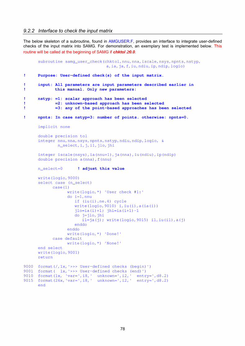
78

9.2.2 Interface to check the input matrix The below skeleton of a subroutine, found in AMGUSER.F, provides an interface to integrate user-defined checks of the input matrix into SAMG. For demonstration, an exemplary test is implemented below. This routine will be called at the beginning of SAMG if chktol ≥0.0.

subroutine samg_user_check(chktol,nnu,nna,iscale,nsys,npnts,nstyp, a,ia,ja,f,iu,ndiu,ip,ndip,logio)

! Purpose: User-defined check(s) of the input matrix. ! input: All parameters are input parameters described earlier in ! this manual. Only new parameters: ! nstyp: =1: scalar approach has been selected ! =2: unknown-based approach has been selected ! =3: any of the point-based approaches has been selected ! npnts: In case nstyp=3: number of points. otherwise: npnts=0.

implicit none

double precision tol integer nnu,nna,nsys,npnts,nstyp,ndiu,ndip,logio, & n_select,i,j,i1,jlo,jhi

integer iscale(nsys),ia(nnu+1),ja(nna),iu(ndiu),ip(ndip) double precision a(nna),f(nnu)

n_select=0 ! adjust this value

write(logio,9000) select case (n_select)

case(1) write(logio,*) 'User check #1:' do i=1,nnu if (iu(i).ne.4) cycle write(logio,9010) i,iu(i),a(ia(i)) jlo=ia(i)+1; jhi=ia(i+1)-1 do j=jlo,jhi i1=ja(j); write(logio,9015) i1,iu(i1),a(j) enddo enddo write(logio,*) 'Done!'

case default write(logio,*) 'None!'

end select write(logio,9001) return

9000 format(/,1x,'>>> User-defined checks (begin)') 9001 format( 1x,'>>> User-defined checks (end)') 9010 format(1x, 'var=',i8,' unknown=',i2,' entry=',d8.2) 9015 format(26x,'var=',i8,' unknown=',i2,' entry=',d8.2)

end

79

9.2.3 Interface to a user's license checker A proper modification of the below dummy routine, contained in AMGUSER.F, provides a means to interface with a user's license checker. This routine is called at the very beginning of SAMG.

subroutine samg_check_license(licensed) ! routine to interface with a user's license checker

implicit none integer licensed licensed=1 ! currently no check done (always satisfied) return end

9.2.4 Interface for getting current cycle number and residual The following interface, contained in AMGUSER.F, allows a user to access the current cycle number and the corresponding residual. This routine is regularly called during the solution phase. Depending on the current values of ncycle and residual, the user may decide to perform some action. Currently, no action is coded:

subroutine samg_current_residual(ncycle,residual)

! provides user-access to current cycle number and residual

implicit none integer ncycle double precision residual

! no action at the moment! return end subroutine samg_current_residual

80

10 Code Numbers of Errors and Warnings In case a fatal error occurred during the execution of SAMG, the program will terminate with a message and the error indicator ierr will return one of the values listed in the following table. In case a non-fatal error occurred, a warning message will be issued but SAMG continues. Upon return from SAMG, ierr will be assigned a negative value (its absolute value corresponds to one of the below error codes).

IERR Description 1 General error (unclassified) 5 Error in license checking

10 Insufficient dimensioning (happens only if memory extension is turned off) 20 Illegal input parameter 30 Undefined or missing input 40 Error in input arrays 50 Incorrect or inconsistent input 51 SAMG re-start terminated: initial call with iswit=4 required 52 SAMG re-start terminated: no AMG decomposition available 53 SAMG re-start terminated: illegal change in parameters 54 SAMG re-start terminated: illegal change in matrix 60 Memory management failed (including file I/O to scratch files) 70 Allocation and de-allocation errors 71 Unexpected allocation status of allocatable array 72 Unexpected assoziation status of pointer array 80 Requested AMG component not installed in current release 90 Logfile exists but could not be opened 91 Logfile already connected to different unit 92 Logfile does not exist and could not be opened 93 Specified unit does not exist 94 Unit=5: Specify a logfile or another unit number

AMG setup 100 General error (unclassified) 101 Setup failed in CNTRL-routine (automatic setup mechanism) 110 Error in defining strong connectivity 120 Error in the splitting process 130 Error in the coarsening process 140 Error in defining interpolation 150 Error in computing the coarse-level Galerkin operators 160 Error in performing the setup optimization

AMG solution phase 200 General error (unclassified) 210 Divergence of the method 220 Error in relaxation (smoothing) 230 Error in ILU (smoothing) 240 Error in ILUT (smoothing) 250 Error in inter-grid transfers 260 Error in alternating �Schwarz process�

81

IERR Description (continued)

300-399 reserved for MPI-parallel SAMG 310 Illegal use of routine in parallel context 320 Illegal use of routine in sequential context

Auxiliary components 800 General error (unclassified) 810 Error in ILU (one-level) 820 Error in ILUT (one-level) 830 Error in conjugate gradient (CG) 831 Quasi residual check has been reached (CG) 832 Residual stagnation check has been reached (CG) 833 Limit of accelerator re-starts has been reached (CG) 840 Error in BiCGstab 841 Quasi residual check has been reached (BiCGstab) 842 Residual stagnation check has been reached (BiCGstab) 843 Limit of accelerator re-starts has been reached (BiCGstab) 855 Error in GMRES 851 Quasi residual check has been reached (GMRES) 852 Residual stagnation check has been reached (GMRES) 853 Limit of accelerator re-starts has been reached (GMRES)

Solution on coarsest level 900 General error (unclassified) 910 Error in method #1 (iterative application of current smoother) 920 Error in method #2 or #4 (preconditioned CG) 930 Error in method #3 or #5 (preconditioned BiCGstab) 960 Error in method #6 (Full Gauss elimination) 970 Error in method #7 (Sparse Gauss elimination) 980 Error in method #8 (Least squares solver) 990 Error in method #9 (user defined solver)

82

11 What is New in this Release? 11.1 Bug fixes

• Bug removed regarding the treatment of the case irestriction_openmp=3. • Error corrected in displaying the parameter ifirst.

11.2 New features

• OpenMP parallelism introduced for most costly parts of SAMG's solution phase. • With the previous SAMG releases it occasionally happened that coarsening was terminated because

two many rows with only positive entries were left on a coarse level. There are new settings available for n_default which continues coaresening by taking such situations into account. In particular, n_default=40 and 42 are recommended as reasonable standard settings.

• Jacobi relaxation has been introduced as a new smoother. • Jacobi block relaxation has been introduced as a new smoother. • Full pivoting of block solvers introduced. • Block ILU has been added as a new smoother. • Various new stopping criteria for SAMG's iteration have been introduced. For instance, it is now

possible to detect when roundoff influence indicates that iteration should be stopped. Also, iterating can be terminated when changes in the solution become too small.

• A limited number of variables can now be forced to strictly remain on the finest level, "decoupled" from the SAMG solution process. Instead, such variables are integrated in the overall solution process via a kind of Schwarz alternating method (with or without overlap).

• There is now an automatic approach aimimg at minimizing the work due to unnecessary setup phases of SAMG. The current version is a prototype, mainly aiming at time stepping methods for which complete setup phases are done only when necessary.

• If the first approximation passed to SAMG already satisifes the stopping criterion defined by eps, SAMG immediately returns.

• The first guess residual - if available before calling SAMG - can now be passed to SAMG so that SAMG does not need to re-compute it.

11.3 New default values

• Calling SAMG with n_default=0 is now equivalent to calling it with n_default=40. • For the simpified SAMG interfaces: iswtch is now initialized to 51 instead of 5199. • The default of check_order is .false.. This is because the consecutive ordering of variables per point

is no longer required. • The default of ilu_speed is 1. That is, by default, ILU is faster but more memory intensive. • The default of lratio is 2. • There are now default values for a_cmplx, g_cmplx, p_cmplx and w_avrge, separately for standard

and aggressive coarsening. 11.4 Other

• The notion of secondary parameters has been removed. All non-primary parameters are now called hidden parameters. The subroutine samg_reset_hidden has been added which resets all hidden parameters to their initial values. However, for reasons of compatibility, the subroutine samg_reset_secondary is still available.

• The concept of one-level methods in the context of SAMG has changed: One-level methods should now (only) be selected by forcing the number of levels to 1 (ie, levelx=1). Although the setting igam>4 is still possible for reasons of compatibility, this way to run one-level methods should not be used any more.

• Empty lines removed in printed output (convergence history on coarser levels).

83

12 References The following gives a list of literature on AMG which is relevant in the context of SAMG. [1-5] give some early references. In particular, [5] contains an extensive description regarding both theory and numerical investigations on AMG. [6-9] are some more recent references. In particular, [8] contains a review on the development of AMG including an extensive list of references. [9] refers to a parallel version of AMG. 1. Brandt, A.; McCormick, S.; Ruge, J.: Algebraic Multigrid (AMG) for Sparse Matrix Equations, in

"Sparsity and its Applications" (D.J. Evans, ed.), Cambridge University Press, pp. 257-284, Cambridge, 1984.

2. Brandt, A.: Algebraic Multigrid Theory: The Symmetric Case, Appl. Math. Comp. 19, pp. 23-56, 1986. 3. Ruge, J.W.; Stüben, K.: Efficient solution of finite difference and finite element equations by algebraic

multigrid (AMG), in Multigrid Methods for Integral and Differential Equations (Paddon, D.J.; Holstein H.; eds.), The Institute of Mathematics and its Applications Conference Series, New Series Number 3, pp. 169-212, Clarenden Press, Oxford, 1985.

4. Stüben, K.: Algebraic multigrid (AMG): Experiences and comparisons, Appl. Math. Comp. 13, pp. 419-

452, 1983. 5. Ruge, J.W.; Stüben, K.: Algebraic Multigrid (AMG), In �Multigrid Methods� (S. McCormick, ed.),

Frontiers in Applied Mathematics, Vol 5, SIAM, Philadelphia 1986. 6. Krechel, A.; Stüben, K.: Operator dependent interpolation in algebraic multigrid, Proceedings of the

Fifth European Multigrid Conference, Stuttgart, Germany, Oct 1-4, 1996. Lecture Notes in Computational Science and Engineering 3, Springer Verlag, 1998. Also available as Arbeitspapier der GMD 1042, January 1997.

7. Stüben, K.: An Introduction to Algebraic Multigrid. Appendix in the book "Multigrid" by U. Trottenberg;

C.W. Oosterlee; A. Schüller. Academic Press, pp. 413-532, 2001. Also available as GMD Report 70, November 1999.

8. Stüben, K.: A Review of Algebraic Multigrid, Journal of Computational and Applied Mathematics

(JCAM) 128, pp. 281-309, 2001 (Volume 7 of JCAM Millenium Issue). Also available as GMD Report 69, November 1999.

9. Krechel, A.; Stüben, K.: Parallel Algebraic Multigrid Based on Subdomain Blocking, Parallel

Computing 27, pp. 1009-1031, 2001. Also available as GMD Report 71, December 1999. 10. Füllenbach, T.; Stüben, K.; Mijalkovic, S.: Application of an algebraic multigrid solver to process

simulation problems, Proceedings of the Intern. Conference on Simulation of Semiconductor Processes and Devices, Seattle (WA), USA, Sep 6-8, 2000. IEEE, Piscataway (NJ), USA, pp. 225-228, 2000.

11. Füllenbach, T.; Stüben, K.: Algebraic multigrid for selected PDE systems, Proceedings of the Fourth

European Conference on Elliptic and Parabolic Problems, Rolduc (The Netherlands) and Gaeta (Italy), 2001. World Scientific, New Jersey, London, pp. 399-410, 2002.

12. Clees, T.; Stüben, K.: Algebraic multigrid for industrial semiconductor device simulation, Proceedings

of the First Intern. Conference on Challenges in Scientific Computing, Berlin, Germany, Oct 2-5, 2002. Lecture Notes in Computational Science and Engineering 35, Springer, Heidelberg, Berlin, 2003.

13. Stüben, K.; Delaney, P.; Chmakov, S.: Algebraic Multigrid (AMG) for Ground Water Flow and Oil

Reservoir Simulation, Proceedings of the Conference �MODFLOW and More 2003: Understanding through Modeling�, International Ground Water Modeling Center (IGWMC), Colorado School of Mines. Golden, Colorado, Sept 17-19, 2003.

14. Clees, T.: AMG Strategies for PDE Systems with Applications in Industrial Semiconductor Simulation.

Ph.D. Thesis, University of Cologne, Nov 30, 2004.

84

13 Index

A

a 22 A(i,j) 14 A[n,m] 13 a_cmplx 35 a_cmplx_agg_default 51 a_cmplx_default 51 acceleration strategies 31 accelerator 31 A-interpolation 27 algebraic multigrid 4 allow_elim 45 alluns_at_allpnts 52 AMG 4 AMG1R5 5 amg1r5_setdble 74 amg1r5_setinteger 74 AMG1R5-like interface 74 amguser.f 21 amguser_nocoo.f 21 argument list 18

B

b_cmplx 45 b_cmplx_agg_default 45 b_cmplx_default 45 backup 65 BiCGstab 9, 11, 31 blk_fillexp 61 blk_stab 61 block coarsening 26 block coupling 14

C

C/F-relaxation 31 C/F-splitting 7 C1-interpolation 27 C2-interpolation 27 CG, conjugate gradient 9, 11, 31 check_allpnts 52 check_order 52 chktol 36 coarse-grid correction 4 coarsening 7, 10 coarsening pattern 71 coarsening strategy 41 coarsening, aggressive 10, 42, 53 coarsening, cluster 10, 42 coarsening, history 37 coarsening, slow 43 coarsening, standard 10, 42 coarsening, very slow 43 coarsest-level solver 7, 11, 31, 49 coarsest-level solver, ILU 49 coarsest-level solver, termination 49 coarsest-level solver, user-supplied 49 complex-valued problems 15 compressed row format 15

console output 36 conv_stop 49 conv_stop_default 49 convergence criteria 56 convergence criteria, approximation based 56 convergence criteria, residual based 56 convergence history on coarser levels 43 coordinates 67 coupled PDE systems 4 coupled system 12 couplings, negative 41 couplings, positive 41 couplings, strong 7, 40 couplings, weak 7 C-relaxation 47 cset_lastpnt 62 cset_lessvars 62 cset_longrow 62 cset_read 62 cset_zerodiag 62 C-variables 7 cycling 11

D

data structure 15 decomposition 7 decomposition, reuse 32 default switch 33 delta_milu 47 densx 43 diagonal dominance 12 diagonal dominance, strong 43 diagonal dominance, strong (local) 40 diagonal dominance, strong violation 40 divergence 65 droptol_cl 50 droptol_smo 47 dummy unknown 16, 27 dump_correctw 46 dumping matrices to disk 70

E

ecg 40 ecg_default 40 ecg1 40 ecg2 40 emergency solver 43 energy norm 70 eps 23, 55 eps_dd 43 eps_diag 44 eps_lsq 68 eps_optrunc 46 error codes 38, 80 errors, fatal 38, 80 errors, non-fatal (warnings) 38, 80 etr 46 etr_default 46 etr1 46 etr2 46 ewt 40

85

ewt_default 40 ewt1 40 ewt2 40

F

f 22 F*-cycle 11 factor_app_var 56 factor_quasi_res 58 factor_res_var 58 F-cycle 8, 31 file access 69 filnam 69 filnam_dump 69 forcing exceptional variables 9 format file, .frm 69 FORTRAN convention 17 frames 70 F-relaxation 47 full_pivoting 50 full_setup 65 F-variables 7 F-variables, exceptional 42

G

g_cmplx 35 g_cmplx_agg_default 51 g_cmplx_default 51 Galerkin 4 Galerkin principle 7 Galerkin, block-diagonal approximation 13, 24 Galerkin, negative diagonal entries 46 Gauss elimination, full 11, 49 Gauss elimination, sparse 11, 49 Gauss-Seidel 10 Gauss-Seidel relaxation, full sweep 47 Gauss-Seidel relaxation, partial sweeps 47 Gauss-Seidel relaxation, symmetric 31, 47 Gauss-Seidel, blockwise 10, 25 Gauss-Seidel, variable-wise 25 geometric coarsening 26 geometric multigrid 4, 8 GMRES 9, 31 graph 12 grid complexity 35 GUI 51

H

hidden parameters 18, 39 hidden parameters, priority 53 hierarchical algorithms 4 history of errors 69 history of residuals 69

I

ia 22 iadp 37 iall 44 iauto_stop 58 iauto_stop_level 58 ib_cmplx 45 ib_cmplx_agg_default 45 ib_cmplx_default 45

ibgs_pivot 47 icdp 37 icheck_quasi_res 58 icrits 56 idmp 37, 70 idump 37, 70 ierr 38 iextent 33 ifirst 23 iforce0 22 igam 31 igdp 37 ignore-warn 65 ILU 25 ILU, blockwise 25 ilu_speed 25, 47 ILUT 25 ILUTP 25 initial memory allocation 35 input matrix checking 36 internal 26 interpolation 7, 10 interpolation, blockwise 24 interpolation, cluster 10 interpolation, direct 10, 44 interpolation, extended standard 10, 44 interpolation, F-relaxation 10 interpolation, Jacobi 10, 44 interpolation, multi-pass 10, 42, 44 interpolation, optimization of 67 interpolation, piecewise constant 10, 42 interpolation, rescaling 44 interpolation, separate 24 interpolation, standard 10, 44 interpolation, the same 24 interpolation, transpose of 7 intlev 44 introduction to AMG 4 iodump 69 ioform 69 iogrid 69 iomovie 69 ioscratch 34 ioscratch_default 51 iounit 72 iout 36 ip 16, 23 ipass_max_set 44 ipriority 59, 60 irestriction_openmp 55 irow0 22 iscale 23 iswit 32, 63, 64 iswtch 32, 33, 34 isym 22 iter_check 50 iter_pre 52 itint 44 itmax_conv 49 itmax_conv_default 49 itypu 23 iu 16, 23 iwdp 37

J

ja 22 Jacobi 10 Jacobi F-relaxation 44

86

Jacobi relaxation 47 Jacobi, blockwise 10

K

Krylov space 31

L

lastgrid 69 least squares 11, 49, 50 levelx 43 levelx, negative sign 43 lfil_cl 49 lfil_cl_default 49 lfil_smo 47 limiting re-starts check 57 linear elasticity 67 logfile 51 logio 51

M

matrix 22 matrix density, maximum 43 max_calls 65 max_cyc 65 max_level 43 maxop_restart 46 memory extension switch 33 memory management 9 memory requirement 9, 10, 35 memory, cleanup routines 20 memory, release 32 messages, cntrl 51 messages, error 51 messages, general 51 messages, warning 51 milu 25, 47 MILU 25 MILUTP 25 mixed-sign rows 41 M-matrices 12 mode_cntrl 65 mode_debug 52 mode_mess 36, 51 multigrid cycle 7, 8, 31 multigrid cycle, optimised corrections 31 multigrid principle 4 multipass_allcoup 45

N

n_default 33, 53 napproach 24 nblk_debug 61 nblk_max 61 nblk_overlap 61 nblk_resid 61 nblk_solve 61 nblk_solver 61 ncframes 69 ncg 41, 42 ncgrad 31 ncgrad_default 31, 51 ncgtyp 41 ncyc 31

ncyc_default 51 ncyc_done 38 ncyc_min 52 ncyc_start 52 ncycle 31, 55 ndim_space 67 ndip 23 ndiu 23 neg_diag 46 neg_diag_brute 46 nfailed_accsteps 58 nint_pat 27 nint_rowsum1 44 nint_weights 27 nkdim 31 nkdim_default 51 nmin_matrix 55 nmin_matrix_resc 55 nmin_vector 55 nna 22 nnu 12, 22 no setup 32 nopt 67 nopt_cforce 68 nopt_fit 68 nopt_split 68 nopt_strong 68 norm, maximum 45 norm, row sum 45 norm, Schur 45 norm_typ 34 normalization 38 norms 23, 34, 38 np_mod1 68 np_mod2 68 np_opt 67 npclass 67 npcol 42 npnts 12, 16 npr_is_dummy 27 nprim 27 nprim_at_allpnts 52 nptmax 43 nptmn 43 nrc 49 nrc_default 49 nrc_emergency 50 nrc_typ 49 nrd 47 nrdtyp 47 nrdx 47 nred 42 nredlev 42 nru 47 nsolve 24, 25, 26, 27 nsolve_default 51 nstrict_ncyc 65 nstrict_quasi 65 nstrict_stagr 65 nstrict_stagu 65 nsys 12, 23 ntake_res_in 52 nth_res_scratch 58 ntr 46 ntrunc 46 num_old_apps 58 num_old_res 58 numtry_max_set 44 nwt 44 nwtint 44

87

nxf_clean 42 nxtyp 25

O

omega_jacobi_default 47 OMP_NUM_THREADS 54 one-level solvers 9, 31, 66 OpenMP 9, 54 OpenMP, fine-tuning 55 operator complexity 35 optimization, level of 67 ordering by points 13 ordering by unknowns 13 ordering, consecutive 16 ordering, pointwise 16 output, suppress all 51

P

P 14 p_cmplx 35 p_cmplx_agg_default 51 p_cmplx_default 51 parallelisation 4 parameters, classes of 18 parameters, hidden 18, 39 parameters, list 18 parameters, primary 18, 22 parameters, set and get routines 18 partial setup 32 partial_frac 65 pattern, SW 27 PDE 4 physical points 12 P-interpolation 27 pivoting, block relaxation 47 plug-in solver 4, 5 point 12 point complexity 35 point-based approaches 13, 16, 24 point-coarsening 13 positive couplings, critical 33 positive couplings, large 40 positive couplings, non-critical 33 preconditioner 8, 9, 31 pre-cycling 31 pre-iteration 31 prim_norm 45 prim_print 45 primary matrix 14, 26 primary matrix, external 26 primary matrix, internal 26 primary matrix, non-zero pattern 26 primary matrix, sparsity pattern 26 primary parameters 5 primary unknown 14, 16, 27 primary_matrix, files 45 print output, I/O unit 51 print output, re-directing 51 print output, setup phase 37 print output, solution phase 36

Q

quasi residual check 57, 58

R

RAMG 5 random function 23 rcondx 50 res_in 38 res_out 38 residual stagnation check 57, 58 residual, quasi 57 residual, real 57 re-start 57 restriction 7 reusing setup data 9 rho_min 65 rho_ok 65 rigid body modes 67

S

s.p.d. 12 saddle point problems 13 safety checks 57 SAMG 5 SAMG with no setup 63, 64 SAMG with partial setup 63, 64 SAMG, simplified interfaces 72 SAMG, standard interface 22 samg_check_license 79 samg_cleanup 20 samg_cntrl_get_xxx 19, 65 samg_cntrl_set_xxx 19, 65 samg_current_residual 79 samg_cvec_alloc 20, 59 samg_cvec_dealloc 20, 59 samg_cvec_set 59 samg_get_xxx 18 samg_getchar 19 samg_getdata 73 samg_getdble 19 samg_getinteger 19 samg_getlogical 19 samg_iget_xxx 19 samg_iset_xxx 19 samg_leave 20 samg_message 51 samg_omega_jacobi_alloc 48 samg_omega_jacobi_dealloc 48 samg_omega_jacobi_set 48 samg_refresh 20, 64 samg_reset_hidden 19, 39 samg_reset_secondary 19 samg_set_xxx 18 samg_setchar 19 samg_setdble 19 samg_setinteger 19 samg_setlogical 19 samg_simple 72 samg_user_check 78 samg_user_cleanup 77 samg_user_coo 21 samg_user_solve 76 scalar approach 12 scalar system 12 scaling 23, 38 Schwarz alternating process 9, 60 Schwarz, block solution 61

88

Schwarz, overlap 60 Schwarz, overlap 1 61 Schwarz, overlap 2 61 Schwarz, subset 60 scratch files 34 setup control mechanism 63 setup control mechanism, interruption 64 setup phase 7 setup phase, automatic control 64 setup phase, manual control 63 show_un_res 52 simple.in 72 slow_coarsening 43 smoothing 4, 7, 10 smoothing strategy 25 smoothing, block ILU 10 smoothing, ILU 10, 25 smoothing, Jacobi 47 smoothing, post- 47 smoothing, pre- 47 solution file, .sol 69 solution phase 7 solution stagnation check 58 solution strategy 24 stability 50 stand-alone 8, 9, 31 state of the art 4 stopping criteria 9, 31, 55 strong connectivity 40, 41 sub-parameters 17 suffix, crw 46

T

term_coarsening 43 termination criteria, coarsening process 43 thread safe 54 threads 54 threshold values 40 time dependent problems 64 transfer operators 7 truncation 10, 46 truncation of Galerkin 10, 46 truncation of interpolation 10, 46

two-level method 8 two-level theory 12 two-part process 7

U

u 22, 38 u(i) 14 u[n] 13 unknown 12 unknown-based approach 13, 16, 24 unstructured mesh 5 user interface, coarsest-level solver 76 user interface, cycle number and residual 79 user interface, input matrix check 78 user interface, license checker 79

V

V*-cycle 11 variable 12 variable-based approach 12, 16, 24 variable-to-coordinate mapping 21 variable-to-point pointer 16, 23 variable-to-unknown pointer 16, 23 V-cycle 8, 31

W

W*-cycle 11 w_avrge 35 w_avrge_agg_default 51 w_avrge_default 51 W-cycle 8, 31 workspace management 20 WW*-cycle 11 WW-cycle 8, 31

Z

zero row sum matrix 22