Use of Local Soil and Vegetation Classifications to ImproveRegional Downstream Hydraulic Geometry Relations

James Bomhof1; Colin D. Rennie, M.ASCE2; and R. Wayne Jenkinson3

Abstract: Regional downstream hydraulic geometry equations are developed using flow with a 1.5-year recurrence interval, and corre-sponding widths, depths, and velocities. The study includes 634 gauge stations located across Canada and are grouped by characteristicsthat affect or are correlated with bank and bed stability. Jack-knife analysis was done to test the predictive capabilities of each grouping. Forwidth prediction, grouping the data by geology and vegetative characteristics improved predictions in 14 of the 15 categories, with drainagecharacteristics and mode of deposition groupings showing the best results. Grouping the data by vegetative characteristics showed the bestimprovement among noncontiguous categories when considering all of the hydraulic geometry variables (width, depth, and velocity). Thesegroupings are investigated further. The study demonstrates that classifying downstream hydraulic geometry equations by local geology andvegetation improves the predictive capabilities of the equations. It also shows that though regionalization does not need to occur in a con-tiguous region, regionalization still provides better results due to the limited resolution of nationally available GIS datasets. As demonstratedin previous studies, it is also shown that downstream hydraulic equations can be applied to semialluvial rivers. Finally, multiple regressionwas tested with width prediction as a function of flow and up to three grouping variables. The interaction of the grouping variables showed noimprovement in the results. DOI: 10.1061/(ASCE)HY.1943-7900.0000978. © 2014 American Society of Civil Engineers.

Introduction

Hydraulic geometry equations were first introduced by Leopoldand Maddock (1953) and built upon the regime theory introducedby Lacey in the 1930s (Lacey 1930). These equations describe hy-draulic variables [surface width (W), mean depth (D), mean veloc-ity (V), roughness (n), slope (S), and suspended sediment load(SL)] as log-linear functions of flow (Q) (Knighton 1998). Theserelationships are defined independently for at-a-station relation-ships and for downstream channel geometry relationships, in whichat-a-station refers to the geometries found at a single cross sectionon a river with varying flow rates, and downstream refers to geom-etries found at multiple cross sections on similar rivers with anequal frequency flow. The downstream hydraulic geometry equa-tions for width, depth, and velocity are shown in Eqs. (1)–(3)

W ¼ aQb ð1Þ

D ¼ cQf ð2Þ

V ¼ kQm ð3Þwhere a, c, k are coefficients; and b, f, m are exponents. Thoughthese empirical relationships have typically been applied to alluvialrivers, studies indicate they can also be applied to semialluvialand nonalluvial rivers (Montgomery and Gran 2001; Wohl 2004;

Ebisa Fola and Rennie 2010; Vachtman and Laronne 2013). The bexponent for width has been found to be almost universally around0.50 for alluvial rivers (Knighton 1998); but this value can varydepending on bank strength and other factors (Anderson et al.2004). While flow is the dominant factor, bank strength also playsan important role in influencing channel geometry and channelpattern (Davies and Sutherland 1980; Osterkamp 1982; Hey andThorne 1986; Huang and Nanson 1998; Millar 2005). Furthermore,vegetation and bank sediment play a large role in determining bankstrength (Huang and Nanson 1998). For example, Ebisa Fola andRennie (2010) found rivers with clay beds and banks to have a bvalue of 0.57. A higher b value indicates that river width increasesmore rapidly with increasing discharge. The U.S. Army Corps ofEngineers (USACE 1994) recommends that streams be designednarrower when there is a higher silt/clay content in the soil becausecohesive properties make the banks less erodible. Cohesive soilsand large materials have high resistance to shear stress, whilemedium-sized particles have low resistance to shear stress (Thorneand Tovey 1981).

Riparian vegetation also has pronounced, but varying, effects onwidth-discharge relationships (Osterkamp 1982). These effects areoften scale dependent (Davies-Colley 1997). Anderson et al. (2004)concluded, after analyzing a large group of datasets, including thatof Davies-Colley (1997), that for small watersheds, stream widthswere greater in forested areas than in unforested areas; and theyconversely found that in larger watersheds, stream widths weresmaller in forested areas than in unforested areas. Eaton and Church(2007) found that relative bank strength declines in the downstreamdirection because the channel depth becomes greater than the root-ing depth of the vegetation. Hey and Thorne (1986) found that thetype and density of riparian vegetation influenced downstreamhydraulic geometry equations in gravel-bed rivers, with greatervegetation density resulting in narrower channels. Copeland et al.(2005) analyzed 57 bankfull width relationships on sand-bed riversand found streams with greater than 50% tree cover had smallerwidths than streams with less than 50% tree cover. Murgatroydand Ternan (1983) found that channel widths within the forest were

1Lake of the Woods Control Board, 373 Sussex Dr., Block E1, Ottawa,ON, Canada K1A 0H3 (corresponding author). E-mail: jbomhof@lwcb.ca

2Dept. of Civil Engineering, Univ. of Ottawa, 161 Louis Pasteur,Ottawa, ON, Canada K1N 6N5. E-mail: crennie@genie.uottawa.ca

3National Research Council, Ocean, Coastal and River Engineering,1200 Montreal Rd., Building M-32, Ottawa, ON, Canada K1A OR6.E-mail: wayne.jenkinson@nrc-cnrc.gc.ca

Note. This manuscript was submitted on November 14, 2013; approvedon October 23, 2014; published online on December 9, 2014. Discussionperiod open until May 9, 2015; separate discussions must be submitted forindividual papers. This paper is part of the Journal of Hydraulic Engineer-ing, © ASCE, ISSN 0733-9429/04014090(10)/$25.00.

© ASCE 04014090-1 J. Hydraul. Eng.

J. Hydraul. Eng.

Dow

nloa

ded

from

asc

elib

rary

.org

by

GE

OR

GIA

TE

CH

LIB

RA

RY

on

12/0

9/14

. Cop

yrig

ht A

SCE

. For

per

sona

l use

onl

y; a

ll ri

ghts

res

erve

d.

up to three times larger than those predicted from the nonforestedcatchment upstream, likely due to within-channel woody debrisdiverting flow toward channel banks and thereby increasing bankerosion. The impact of vegetation on bank strength varies not onlyby the type of vegetation but also by the magnitude of streams.

Bank material composition influences hydraulic geometry(Knighton 1974). Furthermore, it is believed that bank character-istics can be assessed and categorized by determining the surfacegeology and vegetative characteristics along streams. The aim ofthis study is to demonstrate that surficial, geological, and vegetativecharacteristics can be used to develop downstream hydraulicgeometry relationships. To meet this objective, flow measurements,hydraulic geometry data, and surface geology and vegetationmaps were analyzed for all of Canada. Downstream hydraulicgeometry relationships were calculated (1) for all of Canada and(2) after splitting the data set into groups with similar surfacegeology and vegetative characteristics that potentially influencebank strength. This is the first known attempt to assess theinfluence of surficial geology and vegetative characteristics ondownstream hydraulic geometry relations across such a largespatial domain.

Methods

This study primarily relies on two databases provided by Environ-ment Canada (EC) as well as multiple land class geographicinformation system (GIS) databases available through variousgovernment sources. The EC hydrometric database (HYDAT) con-tains daily average flow data for 6,262 active and discontinued hy-drometric gauge stations across Canada dating back to 1860. Thedatabase is publicly available online through the EC website. TheWater Survey of Canada Measurement Database (WSC-MD) wasalso utilized. It was developed for internal use by EnvironmentCanada and contains measured widths, depths, and velocities forvarying flow rates for 1,862 of these stations. These data were origi-nally collected to develop stage-discharge relationships at thesestations.

Publicly available GIS datasets were obtained to classify gaugestations by geologic and vegetative characteristics. Characteristicswere selected on the criteria that nationwide datasets were available

Table 1. NSE Statistics on Regional Downstream Hydraulic Geometry

Classification

NSE Groups withinclassification Category SourceWidth Depth Velocity

Drainage class 0.879 0.761 0.439 6 Geological SLC (1996)Parent material mode of deposition 0.877 0.767 0.506 10 Geological SLC (1996)Surface material (specific) 0.865 0.764 0.419 5 Geological SLC (1996)Calcerous class of parent material 0.863 0.759 0.478 5 Geological SLC (1996)Vegetative land cover 0.861 0.779 0.503 9 Land cover GeoBase (2009)Percentage of rock fragments greater than 0.2 cm (volume) 0.859 0.766 0.525 4 Geological SLC (1996)Geological regions 0.858 0.791 0.598 13 Regional GeoBase (2009)Hydrogeological regions 0.856 0.809 0.614 10 Regional Sharpe et al. (2008)Surficial geology 0.852 0.759 0.479 18 Geological GeoBase (2009)Soil development classification 0.849 0.769 0.491 29 Geological SLC (1996)Surface material (generic) 0.836 0.764 0.470 7 Geological GeoBase (2009)Slope of surrounding region 0.829 0.762 0.518 6 Land cover SLC (1996)No classification 0.795 0.762 0.375 — — —Rooting depth 0.793 0.764 0.460 5 Geological SLC (1996)Random classifications 0.780 0.765 0.370 5 — —

Note: SLC is a national vector dataset with a median polygon size of 221 km2 and polygons as small as 0.0001 km2; Geobase (2009) is a national vectordataset with a median polygon size of 36 km2 and polygons as small as 0.0000003 km2, which maintains a circular map accuracy standard (CMAS) of 30 m orbetter; Geological Survey of Canada (GSC) divides Canada into nine different regions with distinct groundwater systems; it is a vector dataset and noresolution specifications are given.

Fig. 1. Example of at-a-station hydraulic geometry data set and robustregression lines

© ASCE 04014090-2 J. Hydraul. Eng.

J. Hydraul. Eng.

Dow

nloa

ded

from

asc

elib

rary

.org

by

GE

OR

GIA

TE

CH

LIB

RA

RY

on

12/0

9/14

. Cop

yrig

ht A

SCE

. For

per

sona

l use

onl

y; a

ll ri

ghts

res

erve

d.

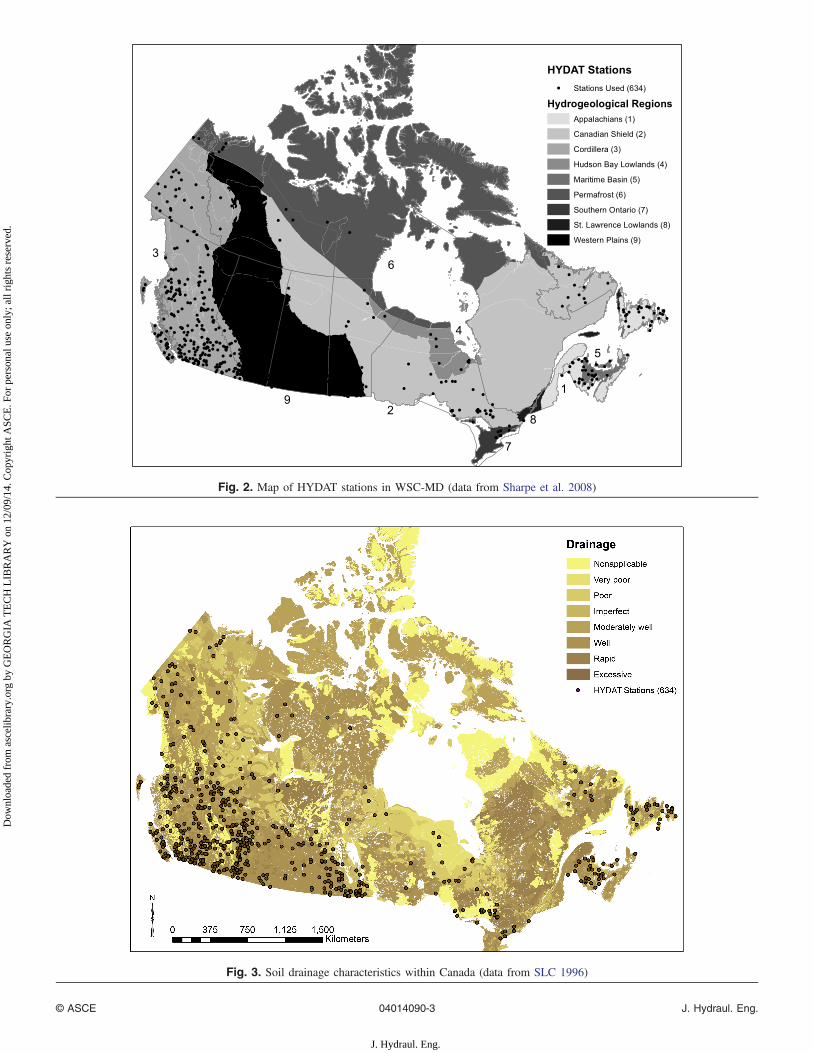
Fig. 2. Map of HYDAT stations in WSC-MD (data from Sharpe et al. 2008)

Fig. 3. Soil drainage characteristics within Canada (data from SLC 1996)

© ASCE 04014090-3 J. Hydraul. Eng.

J. Hydraul. Eng.

Dow

nloa

ded

from

asc

elib

rary

.org

by

GE

OR

GIA

TE

CH

LIB

RA

RY

on

12/0

9/14

. Cop

yrig

ht A

SCE

. For

per

sona

l use

onl

y; a

ll ri

ghts

res

erve

d.

and that the attribute presumably represents bank strength in someform. Soil characteristics were gathered from surficial geologymaps published by the Soil Landscapes of Canada (SLC 1996).The SLC dataset divides Canada into ecodistricts and assigns vari-ous attribute values to each district, including surface material, veg-etative cover, rooting depth, drainage characteristics, surface form,and slope gradient. Land-use data were also found from NaturalResources Canada (GeoBase 2009), which classifies land intonine different types dependant on vegetative characteristics (wet-lands, forest, etc.). The resolution of these datasets is detailed inTable 1.

Bankfull flow is most commonly used in downstream hydraulicgeometry equations (Copeland et al. 2000). Bankfull flow can be(1) measured in the field as the flow at which the water surfaceelevation transitions from the channel to the floodplain, (2) equatedto effective flow, or (3) assumed to occur at a specified flood re-currence interval flow (Copeland et al. 2000). While this recurrenceinterval has been found to have a range of values (Copeland et al.2000; Williams 1978), it has commonly been found to be between 1and 2 years (Harman et al. 1999; Dury 1976; Nixon 1959; Lawlor2004; McCandless 2003). Because it was infeasible to physicallymeasure bankfull flow, and suspended sediment concentrationdata required for calculating effective flow were limited, the1.5-year annual maximum flood was used to approximate bank-full flow.

Because the main intent in creating the WSC-MD was to gatheraccurate flow data, there are biases in the dataset worth discussing.First, the criterion for station locations is based on a number offactors: ease of access, stability of reach, nearby control structures,etc. For the purposes of this study, it is assumed that, despite

the aforementioned biases, the stations in this dataset are arepresentative sample of cross sections in Canadian rivers. It is alsocommon practice, during low flows, for flow and geometry mea-surements to be taken upstream or downstream of the regularlyused station cross section in order to achieve the most accurate flowmeasurement. This problem was pointed out by Park (1977) inregard to United States Geological Survey data.

In order to find W, D, and V at each station for Q1.5, a robust,log-linear regression was applied to the hydraulic geometry datafrom the WSC-MD. This regression is equivalent to developingat-a-station hydraulic geometry curves at each station. Duringthe analysis, the trend of large scatter in the data at lower flowsbecame apparent. This is likely caused by the tendency to usethe optimal cross sections for flow measurement, as previously dis-cussed. Because the data showed more consistency at higher flows,a robust regression was performed on all flows higher than themean annual flow (MAF). Fig. 1 shows an example of an at-a-station analysis. Leopold and Maddock (1953) showed that in orderfor continuity to be maintained, the slopes of the width, depth, andvelocity graphs (b, f, andm) must sum to 1. In the present analysis,any station for which exponents did not sum to 1� 0.05 wasdiscarded. The 5% criterion was also used by Rhodes (1977) as acriterion to include in his triaxial b-f-m diagrams. The averagecontinuity value for these stations was 1.0023 with a standarddeviation of 0.016. Additionally, stations that did not have enoughdata points (<6) were discarded. A map showing the location of the634 sites represented in the filtered dataset is provided in Fig. 2.The filtered stations had an average of 19 geometry measurements.

The study rivers include alluvial rivers, and rivers flowingthrough cohesive sediments or bedrock. Sites represented in the

Fig. 4. Modes of soil deposition within Canada (data from SLC 1996)

© ASCE 04014090-4 J. Hydraul. Eng.

J. Hydraul. Eng.

Dow

nloa

ded

from

asc

elib

rary

.org

by

GE

OR

GIA

TE

CH

LIB

RA

RY

on

12/0

9/14

. Cop

yrig

ht A

SCE

. For

per

sona

l use

onl

y; a

ll ri

ghts

res

erve

d.

filtered dataset were grouped according to local surficial geologyand vegetation characteristics. These characteristics were selectedbased on nationally available datasets whose parameters weremostly likely to be correlated to bank material composition andriparian vegetative characteristics (Table 1). These characteristicsinfluence bank strength. A total of 13 different classifications wereused. Figs. 3 and 4 show maps of Canada classified by soil drainagecharacteristics and parent mode of soil deposition, respectively.The filtered HYDAT stations have been overlayed on the mapsand categorized according to these characteristics. Subsequently,parameters for i ¼ 1∶n result in different regression equations ofthe form

logW ¼ ai þ bi logQ ð4Þwhere n is the number of data subgroups formed for a given char-acteristic map. Multiple regression (MR) was also attempted withup to three categorical variables. All 455 possible combinations ofthe 13 categorical variables (Table 1) were tested. Widths were pre-dicted by multiple regression using the logarithmic form of thedownstream hydraulic geometry equation, as shown in Eq. (5)

logW ¼ ðb × logQþ aÞ þ dC1 þ eC2 þ fC3 ð5Þwhere d, e, f are linear coefficients; and C1, C2, C3 are categoricalvariables.

The models’ predictive capabilities were measured using a jack-knife resampling analysis, also known as a leave-one-out analysis.A subset of the data was taken by omitting a single station. Thedownstream hydraulic geometry equation was calculated on thesubset and then used to predict the geometry of the omitted station.This process was repeated for each station. Observed geometriescould then be compared with estimated geometries. The Nash-Sutcliffe model efficiency coefficient (NSE) was used to assessoverall accuracy of the predicted geometries and is shown inEq. (6) for widths

NSE ¼ 1 −P ðWa −WeÞ2P ðWa −WaÞ2

ð6Þ

whereWa = actual width;We = estimated width; andWa = mean ofall of the actual widths.

The NSE coefficient has a range of −∞ to 1. A value of 1 in-dicates the model has perfect predictive capabilities. An NSE valueless than 0 means that the mean of the observed data is a betterpredictor than the model (Moriasi et al. 2007).

Results

The baseline of the study was set by mapping the downstream hy-draulic geometry equations with no regionalization (Fig. 5). Theterm regionalization is commonly used in the field of hydrologyand refers to the process in which streams are divided into groupsto account for geographic differences. Even without regionalizationa good regression is shown to occur with r2 values of 0.918 and0.817 for width and depth, respectively. However, the verticalscatter about the regression line represents an almost order-of-magnitude variation in channel width and depth for a given dis-charge. The regression for velocity produced a much lower r2

of 0.457. To increase the predictive capability of the observedrelation, regionalization, according to the 13 categorical variablesdescribed earlier, was applied to the downstream hydraulic geom-etry equations.

The NSE results of each regionalization method are shown inTable 1. The results are ordered by NSE values obtained from

the width analysis, and range from 0.780 for random classificationsto 0.879 for classification by drainage class. In the randomclassifications test, the filtered stations were randomly grouped.The inclusion of this test ensured that improved results were notsimply caused by using smaller subsets of data. The baselineresults, where no classification was applied, give an NSE valueof 0.795, the third least effective category. Fig. 6 presents a graphi-cal representation of Table 1, showing the relative NSE improve-ment made by each classification against the baseline result. Anexample of regional downstream hydraulic geometry relationscategorized by soil drainage classifications is shown in Fig. 7.

The best results using the multiple-regression method for widthare shown in Table 2. The highest NSE value recorded was 0.878(Table 2), slightly lower than the best result of the regionalizeddownstream hydraulic geometry approach (Table 1).

Discussion

The 15 characteristics shown in Table 1 can be classified into threemain categories: geological (composition and deposition), land

Fig. 5. Downstream hydraulic geometry at bankfull; the regressionequation exponents for poorly drained and well-drained soils weresignificantly different from the baseline case

© ASCE 04014090-5 J. Hydraul. Eng.

J. Hydraul. Eng.

Dow

nloa

ded

from

asc

elib

rary

.org

by

GE

OR

GIA

TE

CH

LIB

RA

RY

on

12/0

9/14

. Cop

yrig

ht A

SCE

. For

per

sona

l use

onl

y; a

ll ri

ghts

res

erve

d.

cover, and regional characteristics. One can see that the NSE valuefor width increases for almost all of the categories. More impor-tantly, the equations adjust themselves to reflect local conditions.For example, higher b values can be seen in soil with poor drainagecharacteristics (Table 3). Every classification, save rooting depth,shows better predictive results than no classification. The fact thatrandom classifications show worse predictive results demonstratesthat the cause is due to physical reasons and not statistically smallergroupings.

It should be mentioned that the NSE comparative analysis doesnot account for the addition of variables to the model. Models arealmost always improved by additional variables. The models devel-oped in this study modify the original single-regression model byutilizing only a subset of data based on a single categorical group-ing variable. While this may be considered to add an additionalparameter to the model, it is shown that parameterizing (or subset-ting) the model in this way did not necessarily lead to improvedmodel results. Multiple regressions using up to three categoricalvariables did not improve model results, which demonstrated thatadding additional variables to the model was not necessarily ben-eficial. Furthermore, the r2 value for the single-regression modelsin which parameters were fit based on randomly assigned groupswas lower than that of the baseline model, which again demon-strates that the addition of parameters (or subsetting) does notnecessarily improve model results. These results are expected assmaller subsets of data in regression equations can increase the riskof describing the random error in the sample rather than the targetrelationship, which can lead to greater potential for a poorer-performing model. In contrast, developing single-regression equa-tions using a data set defined by a single, well-explained categorical

variable has been shown to defy this trend of increased uncertaintyand improve the predictive capability of the model.

Surficial geology characteristics were shown to influenceregional downstream hydraulic geometry relations. The mostsuccessful categorization for width relations in this study utilizeddrainage class, in which, presumably, low drainage indicated finesoils with minimal pore space. This classification showed an NSEincrease of 0.084 over the baseline model. The specific results fordrainage characteristics are shown in Table 3. Rivers in locationswith poor drainage were found to have higher width exponents,indicating that they become wider more rapidly with increasingQ1.5 discharge. Soil drainage is controlled by topography and soilproperties. In general, drainage will decrease with decreasing porespace. It can thus generally be assumed that poor drainage is cor-related with smaller particle size. Though the a coefficient showsno discernible trend, soils with poorer drainage exhibit higher ratesof width increase (b). The results suggest that rivers flowingthrough poorly drained fine-grained soils are relatively narrow anddeep at small Q1.5 discharges (small creeks and rivers), but becomeincreasingly wide at high Q1.5 discharges (large rivers). In otherwords, it appears that in large rivers the elevated bank strength as-sociated with cohesion of fine-grained soils is insufficient to resistbank erosion and channel widening to accommodate increased dis-charge. This trend may be related to the different erosion processesthat are thought to be prevalent at varying flow scales. It is widelyaccepted that bank erosion occurs slowly through fluvial erosionand rapidly through mass failure (Sutarto et al. 2014). Additionally,Lawler (1992) has argued that mass failure is more likely to be themain mode of bank retreat on the lower reaches of streams. If thesearguments are accepted as true, then the evidence in Table 3

Fig. 6. NSE efficiency improvements on downstream width, depth, and velocity estimation by various regionalization classifications

© ASCE 04014090-6 J. Hydraul. Eng.

J. Hydraul. Eng.

Dow

nloa

ded

from

asc

elib

rary

.org

by

GE

OR

GIA

TE

CH

LIB

RA

RY

on

12/0

9/14

. Cop

yrig

ht A

SCE

. For

per

sona

l use

onl

y; a

ll ri

ghts

res

erve

d.

suggests that rivers found in areas with poor drainage characteris-tics are more likely to experience mass failure than rivers found inwell-drained areas. It is not difficult to imagine that well-drained(and presumably easily erodible) sediments are consistently eroded

over time through fluvial erosion processes and that poorly drained(and presumably cohesive) sediments will erode inconsistently.Observations of bulk erosion of cohesive sediments (Lefebvre et al.1985) and cantilever erosion of composite banks (cohesive upperlayer with alluvial bottom layer) (Thorne and Tovey 1981) are welldocumented in literature. Note that the GIS datasets used in thisstudy only account for the surface layer; it is entirely possible thatrivers in areas classified as having poor drainage could havecomposite banks and hence be susceptible to cantilever erosion.If the stated assumptions are extended to their full conclusion thenthe results in Table 3 also suggest that, over long periods of time,reaches whose dominant erosion is characterized by mass failurewill be wider than reaches dominated by fluvial erosion. Incantilever erosion, periods occur in which gravity forces act in ad-dition to hydraulic forces to erode large portions of the bank over asmall period of time. Once the portion of bank has fallen into thestream, the large exposed surface area of the eroded block willencourage a heightened rate of erosion. While direct observation

W = 4.83Q0.6, r2 = 0.893

1

10

100

1 100 10000

Flow (m3/s)

Wid

th (

m)

Very poor

W = 3.69Q0.57, r2 = 0.926

1

10

100

1 100 10000

Flow (m3/s)

Wid

th (

m)

Poor

W = 4.52Q0.51, r2 = 0.93

1

10

100

1 100 10000

Flow (m3/s)

Wid

th (

m)

Imperfect

W = 4.02Q0.5, r2 = 0.935

1

10

100

1 100 10000

Flow (m3/s)

Wid

th (

m)

Moderately well

W = 5.15Q0.46, r2 = 0.906

1

10

100

1 100 10000

Flow (m3/s)

Wid

th (

m)

Well

W = 4.55Q0.47, r2 = 0.89

1

10

100

1 100 10000

Flow (m3/s)

Wid

th (

m)

Rapid

Fig. 7. Downstream hydraulic geometry with regionalization by drainage characterization

Table 2. NSE Statistics on Downstream Multiple Regression WidthEquations

Classifications NSE

Drainage class, slope of surrounding region, hydrogeologicalregions

0.878

Drainage class, vegetative land cover, surface material (generic) 0.878Drainage class, calcerous class, surface material (specific) 0.878Drainage class, percentage large fragments, hydrogeologicalregions

0.877

Drainage class, calcerous class, hydrogeological regions 0.877Drainage class, calcerous class, slope of surrounding region 0.876Drainage class 0.851

© ASCE 04014090-7 J. Hydraul. Eng.

J. Hydraul. Eng.

Dow

nloa

ded

from

asc

elib

rary

.org

by

GE

OR

GIA

TE

CH

LIB

RA

RY

on

12/0

9/14

. Cop

yrig

ht A

SCE

. For

per

sona

l use

onl

y; a

ll ri

ghts

res

erve

d.

and measurement of this process relative to the continuous fluvialerosion process of a cohesionless substrate would be very difficult,it is plausible that reaches whose bank erosion is dominated bymass failure tend to be wider than reaches whose bank erosion isdominated by fluvial erosion.

Though the lacustrine classification produced a small b expo-nent, the mode of deposition classification for width (Table 4) alsoshowed that streams with cohesive banks have higher b exponents.The first five parameters (alluvial to fluvioglacial) can be summa-rized as larger-grained sediment deposition, likely to have gooddrainage characteristics. On average, the larger-grained sedimentshave lower b values, showing that their widths increase relativelyslowly in the downstream direction. Additionally, their higher aver-age a coefficient causes them to have larger widths at low Q1.5flows. Conversely, the last four parameters are characterized bymud, organic deposition, and rock, having properties of poorerdrainage and higher cohesiveness. Rock channels were found tobe more narrow than alluvial channels for the majority of flows(cf., Wohl and David 2008; Montgomery and Gran 2001).Although the lacustrine classification has more moderate results,this general category has lower initial widths but widths increaserapidly in the downstream direction. On average they showed a20% greater width at high flow (1,000 m3=s) than the larger-grained sediment deposits. One possible reason that the drainageclassification could have produced better and more consistent re-sults is because drainage is an easy and standard variable to mea-sure, whereas other classification measurements are more likely tobe subjective to a certain degree. Surficial geology classificationshave been shown to improve the accuracy of downstream hydraulicgeometry relations and merit further investigation into the physicalmechanisms at work to achieve this improvement.

While geological characteristics showed the most promisingresults in the width regressions, vegetative characteristics had thebest rankings of a spatially noncontiguous classification across allthree hydraulic geometry variables. The intercepts and exponentsfor width, depth, and velocity by classification are shown in Table 5and corresponding values for flow at 10 m3=s (representing small

flow) and 1,000 m3=s (representing large flow) are presented inTable 6. A pattern emerges when looking at the values: cropland,grassland, and wetland tend toward having larger widths and depthsat small flows (<10 m3=s), and corresponding smaller velocities.Forest, shrubland, and barren land have lower widths and depthsat small flows and larger velocities. These results imply that smallerrivers flowing through cropland, grassland, or wetland have lowerslopes and/or greater roughness than rivers flowing through forest,shrubland, or barren land. At large flows the pattern becomesdistorted because, save for velocity, the exponents tend towardequilibrium. This pattern indicates the importance of scale whenconsidering vegetative land cover effects on hydraulic geometry.At large flows the additional bank stability that vegetation initiallyprovides is completely overcome by the larger hydraulic forces.At small-magnitude flows, vegetation with small rooting depths orsubmerged vegetation (wetlands) provides very little additionalbank strength and results in higher overall widths and depths.Conversely, areas covered by forest or shrubland, or which arebarren, indicating a high likelihood of rock outcrops (GeoBase2009), are much less likely to erode, which results in smaller widthsand depths, despite greater streamflow velocities. These results,showing relatively smaller widths in small, forested watersheds,contradict the findings by Anderson et al. (2004) and Murgatroydand Ternan (1983). The bias in the WSC-MD dataset helps toexplain the differences. Murgatroyd and Ternan (1983) suggest themain mechanism for stream widening in forested areas is due tolarge debris within the channel. However, WSC-MD stream datawould have only been recorded in channels free of large debris,thus reducing this stream-widening effect. These results agree withEaton and Church (2007), who state that vegetation’s influence onbank strength will decline in the downstream direction as streamdepths become greater than rooting depths. Interestingly, rootingdepth, which would seem to be a direct indicator of the influenceof vegetation on bank strength, only improved the NSE value ofvelocity estimates.

Multiple regression using classifications showed no improve-ment over the single-classification method. The classificationsincluded in the best multiple-regression model were drainage char-acteristics, slope, and hydrogeological region. As in the classifica-tion analysis (Table 1), drainage characteristics appeared to be themost significant attribute, though when used in the MR equation onits own, it gave an NSE value of only 0.851. The chi-squared testwas used to see if there was correlation between the classificationsin Table 1; however, the tests were inconclusive because the fre-quency of each classification did not meet the minimum standard,typically considered to be 5 (Camilli and Hopkins 1978). WhileNSE results were comparable to those of the classification analysis,including three characteristics in the equation unnecessarily addedcomplexity with no improvement in predictions. Hey and Thorne(1986) and Davies and Sutherland (1980) also used MR and founddischarge to be the dominant variable, while Osterkamp (1982)found more success categorizing downstream hydraulic geometryequations based on sediment type than using MR.

The results show that regional downstream hydraulic equationsdo not need to be defined by a region, although contiguous regionclassifications still result in the best NSE improvement whenconsidering width, depth, and velocity, as shown in Fig. 6. The hy-drogeological regions are defined on the basis of frozen/unfrozenground, bedrock geology, and topography (GeoBase 2009) and areshown in Fig. 2. The idea of using noncontiguous regions is alogical extension of flow regionalization research previously doneby Ouarda et al. (2001) and continued by Jenkinson and Bomhof(2012). It was shown that historical flows could be better predictedusing canonical-correlation analysis as a regionalization technique,

Table 3. Downstream Width Parameters Grouped by Drainage Conditions

Drainage condition a b r2 Stations

Very poor 4.84 0.605 0.808 10Poor 3.69a 0.567a 0.923 31Imperfect 4.52 0.506 0.929 86Moderately well 4.02a 0.504a 0.934 119Well 5.15a 0.462a 0.906 305Rapid 4.55 0.470 0.888 55aDenotes a value significantly different than the mean value at a 95%confidence.

Table 4. Downstream Width Parameters Grouped by Mode of Deposition

Mode of deposition a b r2 Stations

Alluvial 5.15 0.479 0.931 38Colluvial 4.19 0.468 0.918 75Eolian 4.39 0.510 0.885 7Morainal 4.61 0.487 0.909 272Fluvioglacial 5.35a 0.450 0.899 62Lacustrine 5.42 0.463a 0.882 110Marine 3.77 0.491 0.938 7Organic 3.71 0.600 0.837 21Rock 3.59 0.524 0.866 21aDenotes a value significantly different than the mean value at a 95%confidence.

© ASCE 04014090-8 J. Hydraul. Eng.

J. Hydraul. Eng.

Dow

nloa

ded

from

asc

elib

rary

.org

by

GE

OR

GIA

TE

CH

LIB

RA

RY

on

12/0

9/14

. Cop

yrig

ht A

SCE

. For

per

sona

l use

onl

y; a

ll ri

ghts

res

erve

d.

which does not assume that neighboring streams need to lie in acontiguous area, only that they have similar watershed character-istics. The result is a regional hydraulic geometry relation in whichthe region is defined by the local surficial geology and vegetationcharacteristics, not necessarily geographic location. This is similarin concept to traditional hydraulic geometry relations developedfor rivers with specific bed material (e.g., sand versus gravel).The advantages of the present approach are that a large varietyof local sediment and vegetation characteristics that influence bankstrength can be considered, and these characteristics are readilyavailable over large spatial domains. However, contiguous regionclassifications were most successful at improving relations for allthree variables: width, depth, and velocity. Thus, it appears bank-strength-specific hydraulic geometry relations can be generatedover large domains. It appears that contiguous regions in hydraulicdownstream equations remain the most practical approach becausethe resolution of GIS datasets is not yet able to meet the stringentrequirements for adequately determining bank strength. The criticaldifference between the regionalization techniques for hydrologyversus hydraulic applications is that the resolution is more adequatefor hydrological purposes because the GIS information is averagedover the entire watershed. The authors suggest that the noncontigu-ous method of regionalization of downstream hydraulic equationswill become more practical with time as the resolution of remotesensing data over large spatial domains is improved.

This analysis also demonstrates that downstream hydraulicgeometry can be extended to semialluvial streams. Traditionally,these equations have been applied to streams whose floodplainsare made up of the same material that the river carries. Due tothe vast variety of geographic landforms in Canada, a large portionof Canadian streams cannot be considered alluvial. Rivers in theRocky Mountains or in the Canadian Shield are highly likely tobe restricted by bedrock, while rivers in the lacustrine sedimentof eastern Ontario are likely to be restricted by cohesive clay banks.Though some studies did not find a strong relationship, Ponton(1972), Montgomery and Gran (2001), Wohl (2004), and Molnarand Ramirez (2002) have shown that downstream hydraulicgeometry relationships can be applied to mountain rivers, whileEbisa Fola and Rennie (2010) showed that downstream hydraulic

geometry equations can be applied to cohesive soils. These empiri-cal results could possibly be explained by the stream power of theserivers. Wohl (2004) found that downstream hydraulic geometry re-lationships were better developed if the stream power to sedimentsize ratio dropped below 10,000 kg=s3. Successful demonstrationsof this extension of downstream hydraulic geometry merit furtherinvestigation for possible explanations of this phenomenon.

Conclusions

Regionalization of downstream hydraulic geometry equations bygeological and vegetative characteristics, as well as regional geol-ogy classifications, improved the predictive capabilities of theseequations. It was shown that prediction improvements of 8.4,4.8, and 23.9% could be achieved for width, depth, and averagevelocities, respectively. Geological characteristics, particularlydrainage characteristics and mode of deposition, were found to im-prove the width predictions best. It is argued that improvement islikely caused by the correlation of drainage characteristics withparticle size and, therefore, that it provides an indication of bankstrength. Classifications indicating cohesive sediments had higherb exponents, showing that large rivers flowing through cohesivematerial can be relatively wide. Vegetative classifications showedthe best improvement for a noncontiguous classification acrosswidth, depth, and velocity. Results showed that for small water-sheds, widths and depths were smaller in forested areas than ingrasslands, and that vegetative influence on hydraulic geometryis reduced as flows increase. The contiguous classification ofhydrogeological regions, indicating major groundwater regionswithin Canada, showed the best improvement for all three hydraulicgeometry equations. This is likely because the spatial resolution ofnationally available GIS datasets is still limited compared to therelatively small area of a river cross section. There is great potentialfor improvement in regionalization by noncontiguous vegetationand geological characteristics as the resolution of these datasets im-proves. Multiple regressions using flow and up to three categoricalvariables as independent variables were also attempted but showedno improvement over the classical regionalization methods. Finally,the results demonstrate that downstream hydraulic geometry equa-tions can be applied to semialluvial rivers.

Acknowledgments

The authors wish to thank the anonymous reviewers and the editorsfor their helpful comments that improved the paper.

References

Anderson, R. J., Bledsoe, B. P., and Hession, W. C. (2004). “Width ofstreams and rivers in response to vegetation, bank material, and otherfactors.” J. Am. Water Resour. Assoc., 40(5), 1159–1172.

Table 6. Downstream Hydraulic Geometry Values Grouped by VegetativeLand Cover

Land coverWsmall(m)

Wlarge(m)

Dsmall(m)

Dlarge(m)

Vsmall(m=s)

V large(m=s)

Cropland 15.85 118.29 0.88 4.17 0.72 1.99Grassland 15.95 130.29 0.81 3.67 0.77 2.07Wetland 16.13 170.23 0.95 3.06 0.73 1.60Forest 13.11 125.85 0.70 3.59 1.13 2.20Shrubland 12.52 132.72 0.68 3.28 1.15 2.27Barren 11.95 137.91 0.81 3.56 1.07 2.09

Note: Small is represented by a 10 m3=s flow; large is represented by a1,000 m3=s flow.

Table 5. Downstream Hydraulic Geometry Parameters Grouped by Vegetative Land Cover

Land cover a B r2 c F r2 k m r2 Stations

Cropland 5.80a 0.436a 0.849 0.403a 0.338 0.727 0.429a 0.222 0.532 75Grassland 5.58a 0.456a 0.932 0.383 0.327 0.801 0.470a 0.215 0.512 63Wetland 4.97 0.512 0.878 0.529 0.254 0.529 0.496 0.169 0.174 14Forest 4.23a 0.491 0.899 0.307a 0.356a 0.825 0.809a 0.145 0.357 261Shrubland 3.85a 0.513 0.951 0.313a 0.340 0.899 0.814a 0.148 0.445 28Barren 3.52 0.531 0.875 0.387 0.321 0.719 0.764 0.146 0.225 28aDenotes a value significantly different than the mean value at a 95% confidence.

© ASCE 04014090-9 J. Hydraul. Eng.

J. Hydraul. Eng.

Dow

nloa

ded

from

asc

elib

rary

.org

by

GE

OR

GIA

TE

CH

LIB

RA

RY

on

12/0

9/14

. Cop

yrig

ht A

SCE

. For

per

sona

l use

onl

y; a

ll ri

ghts

res

erve

d.

Camilli, G., and Hopkins, K. D. (1978). “Applicability of chi-square to2 × 2 contingency tables with small expected cell frequencies.”Psychol. Bull., 85(1), 163–167.

Copeland, R. R., Biedenharn, D. S., and Fischenich, J. C. (2000).“Channel-forming discharge.” U.S. Army Corps of Engineers TechnicalNote, Engineer Research and Development Center Coastal andHydraulics Lab (ERDC/CHL CHETN-VIII-5, 1-11), Vicksburg, MS.

Copeland, R., Soar, P., and Thorne, C. (2005). “Channel-forming dischargeand hydraulic geometry width predictors in meandering sandbedrivers.” Proc., 2005 World Water and Environmental ResourcesCongress: Impacts of Global Change, ASCE, Reston, VA.

Davies, T., and Sutherland, A. (1980). “Resistance to flow past deformableboundaries.” Earth Surf. Processes, 5(2), 175–179.

Davies-Colley, R. J. (1997). “Stream channels are narrower in pasture thanin forest.” N. Z. J. Mar. Freshwater Res., 31(5), 599–608.

Dury, G. (1976). “Discharge prediction, present and former, from channeldimensions.” J. Hydrol., 30(3), 219–245.

Eaton, B., and Church, M. (2007). “Predicting downstream hydraulicgeometry: A test of rational regime theory.” J. Geophys. Res. EarthSurf., 112(F3), in press.

Ebisa Fola, M., and Rennie, C. D. (2010). “Downstream hydraulic geom-etry of clay-dominated cohesive bed rivers.” J. Hydraul. Eng., 136(8),524–527.

GeoBase. (2009). Land cover, circa 2000-vector, Centre for TopographicInformation Earth Sciences Sector, Sherbrook, QC, Canada.

Harman, W., et al. (1999). “Bankfull hydraulic geometry relationships forNorth Carolina streams.” Proc., American Water Resources AssociationSpecialty Conf., Wildland Hydrology, 401–408.

Hey, R., and Thorne, C. (1986). “Stable channels with mobile gravel beds.”J. Hydraul. Eng., 112(8), 671–689.

Huang, H., and Nanson, G. (1998). “The influence of bank strength onchannel geometry: An integrated analysis of some observations.” EarthSurf. Processes Landforms, 23(10), 865–876.

Jenkinson, R. W., and Bomhof, J. (2012). “Assessment of Canada’s hydro-kinetic power potential—Phase II methodology validation.” TechnicalRep., National Research Council—Ocean Coastal and River Engineer-ing, Ottawa, ON, Canada.

Knighton, D. (1974). “Variation in width-discharge relation and someimplications for hydraulic geometry.” Geol. Soc. Am. Bull., 85(7),1069–1076.

Knighton, D. (1998). Fluvial forms and processes: A new perspective,Wiley, New York.

Lacey, G. (1930). “Stable channels in alluvium.” Inst. Civil Eng. Proc., 229,259–384.

Lawler, D. M. (1992). “Process dominance in bank erosion.” Lowlandfloodplain rivers: Geomorphological perspectives, Wiley, Chichester,England, 117–143.

Lawlor, S. M. (2004). “Determination of channel-morphology characteris-tics, bankfull discharge, and various design-peak discharges in westernMontana.” U.S. Geological Survey Scientific Investigations Rep. 2004-5263, Reston, VA, 19.

Lefebvre, G., Rohan, K., and Douville, S. (1985). “Erosivity of natural in-tact structured clay: Evaluation.” Can. Geotech. J., 22.4(252), 508–517.

Leopold, L. B., and Maddock, T. (1953). “The hydraulic geometry ofstream channels and some physiographic implications.” U.S. GeologicalSurvey Professional Paper No. 252, U.S. Government Printing Office,Washington, DC, 57.

McCandless, T. (2003). “Maryland stream survey: Bankfull discharge andchannel characteristics of streams in the Allegheny Plateau and thevalley and ridge hydrologic regions.” Chesapeake Bay Field Office-S03-01, U.S. Fish and Wildlife Service, Annapolis, MD.

Millar, R. (2005). “Theoretical regime equations for mobile gravel-bedrivers with stable banks.” Geomorphology, 64(3), 207–220.

Molnar, P., and Ramirez, J. A. (2002). “On downstream hydraulic geometryand optimal energy expenditure: Case study of the Ashley and Taieririvers.” J. Hydrol., 259(1), 105–115.

Montgomery, D., and Gran, K. (2001). “Downstream variations in thewidth of bedrock channels.” Water Resour. Res., 37(6), 1841–1846.

Moriasi, D., Arnold, J., Van Liew, M., Bingner, R., Harmel, R., and Veith,T. (2007). “Model evaluation guidelines for systematic quantification ofaccuracy in watershed simulations.” Trans. ASABE, 50(3), 885–900.

Murgatroyd, A., and Ternan, J. (1983). “The impact of afforestation onstream bank erosion and channel form.” Earth Surf. ProcessesLandforms, 8(4), 357–369.

Nixon, M. (1959). “A study of the bank-full discharges of rivers in Englandand Wales.” ICE Proc., Vol. 12, 157–174.

Osterkamp, W. (1982). “Perennial-streamflow characteristics related tochannel geometry and sediment in Missouri River basin.” U.S. Geologi-cal Survey Professional Paper, Alexandria, VA, 37.

Ouarda, T. B. M. J., Girard, C., Cavadias, G. S., and Bobée, B. (2001).“Regional flood frequency estimation with canonical correlationanalysis.” J. Hydrol., 254(1–4), 157–173.

Park, C. C. (1977). “World-wide variations in hydraulic geometryexponents of stream channels: An analysis and some observations.”J. Hydrol., 33(1), 133–146.

Ponton, J. R. (1972). “Hydraulic geometry in the Green and Birkenheadbasins, British Columbia.”Mountain geomorphology: Geomorphologi-cal processes in the Canadian Cordillera, H. O. Slaymaker and H. J.McPherson, eds., Tantalus Research, Vancouver, Canada, 151–160.

Rhodes, D. (1977). “The bfm diagram: Graphical representation andinterpretation of at-a-station hydraulic geometry.” Am. J. Sci., 277,73–95.

Sharpe, D., Russell, H., Grasby, S., and Wozniak, P. (2008). “Hydrogeo-logical regions of Canada: Data release. Geological survey of Canada(GSC).” Open File 5893, Sherbrook, QC, Canada, 20.

SLC (Soil Landscapes of Canada). (1996). Soil landscapes of Canada(SLC), Centre for Land and Biological Resources Research, Ottawa,ON, Canada.

Sutarto, T., Papanicolaou, A. N., Wilson, C. G., and Langendoen, E. J.(2014). “Stability analysis of semicohesive streambanks with concepts:Coupling field and laboratory investigations to quantify the onset offluvial erosion and mass failure.” J. Hydraul. Eng., 140(9), 04014041.

Thorne, C. R., and Tovey, N. K. (1981). “Stability of composite riverbanks.” Earth Surf. Processes Landforms, 6(5), 469–484.

USACE (U.S. Army Corps of Engineers). (1994). Channel stabilityassessment for flood control projects, Washington, DC.

Vachtman, D., and Laronne, J. B. (2013). “Hydraulic geometry of cohesivechannels undergoing base level drop.” Geomorphology, 197, 76–84.

Williams, G. P. (1978). “Bank-full discharge of rivers.”Water Resour. Res.,14(6), 1141–1154.

Wohl, E. (2004). “Limits of downstream hydraulic geometry.” Geology,32(10), 897–900.

Wohl, E., and David, G. (2008). “Consistency of scaling relations amongbedrock and alluvial channels.” J. Geophys. Res., 113(F4), F04013.

© ASCE 04014090-10 J. Hydraul. Eng.

J. Hydraul. Eng.

Dow

nloa

ded

from

asc

elib

rary

.org

by

GE

OR

GIA

TE

CH

LIB

RA

RY

on

12/0

9/14

. Cop

yrig

ht A

SCE

. For

per

sona

l use

onl

y; a

ll ri

ghts

res

erve

d.