This is an electronic reprint of the original article.This reprint may differ from the original in pagination and typographic detail.

Powered by TCPDF (www.tcpdf.org)

This material is protected by copyright and other intellectual property rights, and duplication or sale of all or part of any of the repository collections is not permitted, except that material may be duplicated by you for your research use or educational purposes in electronic or print form. You must obtain permission for any other use. Electronic or print copies may not be offered, whether for sale or otherwise to anyone who is not an authorised user.

MAGIC Collaboration; Hovatta, T.; Lähteenmäki, A.; Tornikoski, M.; Tammi, J.;Ramakrishnan, V.Unraveling the Complex Behavior of Mrk 421 with Simultaneous X-Ray and VHEObservations during an Extreme Flaring Activity in 2013 April

Published in:Astrophysical Journal, Supplement Series

DOI:10.3847/1538-4365/ab89b5

Published: 01/06/2020

Document VersionPublisher's PDF, also known as Version of record

Please cite the original version:MAGIC Collaboration, Hovatta, T., Lähteenmäki, A., Tornikoski, M., Tammi, J., & Ramakrishnan, V. (2020).Unraveling the Complex Behavior of Mrk 421 with Simultaneous X-Ray and VHE Observations during anExtreme Flaring Activity in 2013 April. Astrophysical Journal, Supplement Series, 248(2), [29].https://doi.org/10.3847/1538-4365/ab89b5

Unraveling the Complex Behavior of Mrk 421 with Simultaneous X-Ray and VHEObservations during an Extreme Flaring Activity in 2013 April*

V. A. Acciari1 , S. Ansoldi2,3 , L. A. Antonelli4 , A. Arbet Engels5 , D. Baack6 , A. Babić7 , B. Banerjee8 ,U. Barres de Almeida9 , J. A. Barrio10 , J. Becerra González1 , W. Bednarek11 , L. K. Bellizzi12, E. Bernardini13,14 ,

A. Berti15 , J. Besenrieder16, W. Bhattacharyya13 , C. Bigongiari4 , A. Biland5 , O. Blanch17 , G. Bonnoli12 ,Ž. Bošnjak7 , G. Busetto14 , R. Carosi18 , G. Ceribella16, M. Cerruti19 , Y. Chai16 , A. Chilingarian20 , S. Cikota7,

S. M. Colak17 , U. Colin16, E. Colombo1 , J. L. Contreras10 , J. Cortina21 , S. Covino4 , V. D’Elia4 , P. Da Vela18,63,F. Dazzi4 , A. De Angelis14 , B. De Lotto2 , F. Del Puppo2, M. Delfino17,64 , J. Delgado17,64 , D. Depaoli15 ,

F. Di Pierro15 , L. Di Venere15 , E. Do Souto Espiñeira17 , D. Dominis Prester7 , A. Donini2 , D. Dorner22 , M. Doro14 ,D. Elsaesser6 , V. Fallah Ramazani23,24 , A. Fattorini6, G. Ferrara4 , L. Foffano14 , M. V. Fonseca10 , L. Font25 ,C. Fruck16 , S. Fukami3, R. J. García López1 , M. Garczarczyk13 , S. Gasparyan20, M. Gaug25 , N. Giglietto15 ,

F. Giordano15 , P. Gliwny11 , N. Godinović7 , D. Green16 , D. Hadasch3 , A. Hahn16 , T. Hassan13,17 , J. Herrera1 ,J. Hoang10 , D. Hrupec7 , M. Hütten16 , T. Inada3, S. Inoue3 , K. Ishio16, Y. Iwamura3, L. Jouvin17 , Y. Kajiwara3,D. Kerszberg17 , Y. Kobayashi3, H. Kubo3 , J. Kushida3 , A. Lamastra4 , D. Lelas7 , F. Leone4 , E. Lindfors23,24 ,

S. Lombardi4 , F. Longo2,65 , M. López10 , R. López-Coto14 , A. López-Oramas1 , S. Loporchio15 ,B. Machado de Oliveira Fraga9 , C. Maggio25 , P. Majumdar8 , M. Makariev26 , M. Mallamaci14 , G. Maneva26 ,M. Manganaro7 , K. Mannheim22 , L. Maraschi4, M. Mariotti14 , M. Martínez17 , D. Mazin3,16 , S. Mender6 ,

S. Mićanović7 , D. Miceli2 , T. Miener10, M. Minev26, J. M. Miranda12 , R. Mirzoyan16 , E. Molina19 , A. Moralejo17 ,D. Morcuende10 , V. Moreno25 , E. Moretti17 , P. Munar-Adrover25 , V. Neustroev23,24 , C. Nigro13 , K. Nilsson23,24 ,

D. Ninci17 , K. Nishijima3 , K. Noda3 , L. Nogués17 , S. Nozaki3 , Y. Ohtani3, T. Oka3 , J. Otero-Santos1 ,M. Palatiello2 , D. Paneque3,16 , R. Paoletti12 , J. M. Paredes19 , L. Pavletić7 , P. Peñil10, M. Peresano2 , M. Persic2,66 ,P. G. Prada Moroni18 , E. Prandini14 , I. Puljak7 , W. Rhode6 , M. Ribó19 , J. Rico17 , C. Righi4 , A. Rugliancich18 ,

L. Saha10 , N. Sahakyan20 , T. Saito3, S. Sakurai3, K. Satalecka13 , B. Schleicher22, K. Schmidt6 , T. Schweizer16 ,J. Sitarek11, I. Šnidarić7, D. Sobczynska11 , A. Spolon14 , A. Stamerra4 , D. Strom16 , M. Strzys3, Y. Suda16 , T. Surić7,

M. Takahashi3 , F. Tavecchio4 , P. Temnikov26 , T. Terzić7 , M. Teshima3,16, N. Torres-Albà19 , L. Tosti15,J. van Scherpenberg16 , G. Vanzo1 , M. Vazquez Acosta1 , S. Ventura12 , V. Verguilov26 , C. F. Vigorito15 ,

V. Vitale15 , I. Vovk16 , M. Will16 , D. Zarić7 ,(MAGIC Collaboration)

Othergroupsandcollaborators:,M. Petropoulou27 , J. Finke28 , F. D’Ammando29 , M. Baloković30,31 , G. Madejski32, K. Mori33, Simonetta Puccetti34,C. Leto35, M. Perri35,36, F. Verrecchia35,36 , M. Villata37 , C. M. Raiteri37 , I. Agudo38 , R. Bachev39, A. Berdyugin40,D. A. Blinov41,42,43, R. Chanishvili44, W. P. Chen45, R. Chigladze44, G. Damljanovic46, C. Eswaraiah45, T. S. Grishina41,

S. Ibryamov39, B. Jordan47, S. G. Jorstad41,48 , M. Joshi41, E. N. Kopatskaya41, O. M. Kurtanidze44,49,50 , S. O. Kurtanidze44,E. G. Larionova41, L. V. Larionova41, V. M. Larionov41,51, G. Latev39, H. C. Lin45, A. P. Marscher48 , A. A. Mokrushina41,51,D. A. Morozova41, M. G. Nikolashvili44, E. Semkov39, P. S. Smith52, A. Strigachev39, Yu. V. Troitskaya41, I. S. Troitsky41,

O. Vince46, J. Barnes53, T. Güver54 , J. W. Moody55, A. C. Sadun56, T. Hovatta57,58 , J. L. Richards59, W. Max-Moerbeck60 ,A. C. S. Readhead61, A. Lähteenmäki58,62, M. Tornikoski58 , J. Tammi58, V. Ramakrishnan58, and R. Reinthal401 Inst. de Astrofísica de Canarias, E-38200 La Laguna, and Universidad de La Laguna, Dpto. Astrofísica, E-38206 La Laguna, Tenerife, Spain

2 Università di Udine, and INFN Trieste, I-33100 Udine, Italy3 Japanese MAGIC Consortium: ICRR, The University of Tokyo, 277-8582 Chiba, Japan; Department of Physics, Kyoto University, 606-8502 Kyoto; Tokai

University, 259-1292 Kanagawa, Japan; RIKEN, 351-0198 Saitama, Japan;4 National Institute for Astrophysics (INAF), I-00136 Rome, Italy

5 ETH Zurich, CH-8093 Zurich, Switzerland6 Technische Universität Dortmund, D-44221 Dortmund, Germany

7 Croatian Consortium: University of Rijeka, Department of Physics, 51000 Rijeka; University of Split—FESB, 21000 Split; University of Zagreb—FER, 10000Zagreb; University of Osijek, 31000 Osijek; Rudjer Boskovic Institute, 10000 Zagreb, Croatia; ana.babic@fer.hr

8 Saha Institute of Nuclear Physics, HBNI, 1/AF Bidhannagar, Salt Lake, Sector-1, Kolkata 700064, India9 Centro Brasileiro de Pesquisas Físicas (CBPF), 22290-180 URCA, Rio de Janeiro (RJ), Brasil

10 IPARCOS Institute and EMFTEL Department, Universidad Complutense de Madrid, E-28040 Madrid, Spain11 University of Lodz, Faculty of Physics and Applied Informatics, Department of Astrophysics, 90-236 Lodz, Poland

12 Università di Siena and INFN Pisa, I-53100 Siena, Italy13 Deutsches Elektronen-Synchrotron (DESY), D-15738 Zeuthen, Germany; thassan@ifae.es

14 Università di Padova and INFN, I-35131 Padova, Italy15 Istituto Nazionale Fisica Nucleare (INFN), I-00044 Frascati (Roma), Italy

16 Max-Planck-Institut für Physik, D-80805 München, Germany; dpaneque@mppmu.mpg.de17 Institut de Física d’Altes Energies (IFAE), The Barcelona Institute of Science and Technology (BIST), E-08193 Bellaterra (Barcelona), Spain

18 Università di Pisa, and INFN Pisa, I-56126 Pisa, Italy

The Astrophysical Journal Supplement Series, 248:29 (36pp), 2020 June https://doi.org/10.3847/1538-4365/ab89b5© 2020. The American Astronomical Society. All rights reserved.

* Contact MAGIC Collaboration (contact.magic@mpp.mpg.de) for queries. Corresponding authors are D. Paneque, A. Babic, J. Finke, T. Hassan, andM. Petropoulou.

1

19 Universitat de Barcelona, ICCUB, IEEC-UB, E-08028 Barcelona, Spain20 The Armenian Consortium: ICRANet-Armenia at NAS RA, A. Alikhanyan National Laboratory, Armenia

21 Centro de Investigaciones Energéticas, Medioambientales y Tecnológicas, E-28040 Madrid, Spain22 Universität Würzburg, D-97074 Würzburg, Germany

23 Finnish MAGIC Consortium: Finnish Centre of Astronomy with ESO (FINCA), University of Turku, FI-20014 Turku, Finland24 Astronomy Research Unit, University of Oulu, FI-90014 Oulu, Finland

25 Departament de Física, and CERES-IEEC, Universitat Autònoma de Barcelona, E-08193 Bellaterra, Spain26 Inst. for Nucl. Research and Nucl. Energy, Bulgarian Academy of Sciences, BG-1784 Sofia, Bulgaria

27 Princeton University, Princeton NJ, USA; m.petropoulou@astro.princeton.edu28 US Naval Research Laboratory, Washington DC, USA; justin.finke@nrl.navy.mil

29 INAFIstituto di Radioastronomia, Via P. Gobetti 101, I-40129 Bologna, Italy30 Center for Astrophysics | Harvard & Smithsonian, 60 Garden Street, Cambridge, MA 02138, USA

31 Black Hole Initiative at Harvard University, 20 Garden Street, Cambridge, MA 02138, USA32 W.W. Hansen Experimental Physics Laboratory, Kavli Institute for Particle Astrophysics and Cosmology, Department of Physics and SLAC National Accelerator

Laboratory, Stanford University, Stanford, CA 94305, USA33 Columbia Astrophysics Laboratory, 550 W 120th St. New York, NY 10027, USA

34 Agenzia Spaziale Italiana (ASI)-Unita’ di Ricerca Scientifica, Via del Politecnico, I-00133 Roma, Italy35 ASI Science Data Center, Via del Politecnico snc I-00133, Roma, Italy

36 INAF—Osservatorio Astronomico di Roma, via di Frascati 33, I-00040 Monteporzio, Italy37 INAF—Osservatorio Astrofisico di Torino, I-10025 Pino Torinese (TO), Italy

38 Instituto de Astrofísica de Andalucía (CSIC), Apartado 3004, E-18080 Granada, Spain39 Institute of Astronomy and National Astronomical Observatory, Bulgarian Academy of Sciences, 72 Tsarigradsko shosse Blvd., 1784 Sofia, Bulgaria

40 Tuorla Observatory, Department of Physics and Astronomy, Väisäläntie 20, FI-21500 Piikkiö, Finland41 Astronomical Institute, St. Petersburg State University, Universitetskij Pr. 28, Petrodvorets, 198504 St. Petersburg, Russia

42 Department of Physics and Institute for Plasma Physics, University of Crete, 71003, Heraklion, Greece43 Foundation for Research and Technology—Hellas, IESL, Voutes, 71110 Heraklion, Greece

44 Abastumani Observatory, Mt. Kanobili, 0301 Abastumani, Georgia45 Graduate Institute of Astronomy, National Central University, 300 Zhongda Road, Zhongli 32001, Taiwan

46 Astronomical Observatory, Volgina 7, 11060 Belgrade, Serbia47 School of Cosmic Physics, Dublin Institute For Advanced Studies, Ireland

48 Institute for Astrophysical Research, Boston University, 725 Commonwealth Avenue, Boston, MA 02215, USA49 Engelhardt Astronomical Observatory, Kazan Federal University, Tatarstan, Russia

50 Center for Astrophysics, Guangzhou University, Guangzhou 510006, Peopleʼs Republic of China51 Pulkovo Observatory, St.-Petersburg, Russia

52 Steward Observatory, University of Arizona, 933 N. Cherry Avenue, Tucson, AZ 85721, USA53 Department of Physics, Salt Lake Community College, Salt Lake City, UT 84070, USA

54 Istanbul University, Science Faculty, Department of Astronomy and Space Sciences, Beyazıt, 34119, Istanbul, Turkey55 Department of Physics and Astronomy, Brigham Young University, Provo, UT 84602 USA

56 Department of Physics, University of Colorado Denver, Denver, Colorado, CO 80217-3364, USA57 Finnish Centre for Astronomy with ESO (FINCA), University of Turku, FI-20014 Turku, Finland58 Aalto University, Metsähovi Radio Observatory, Metsähovintie 114, FI-02540 Kylmälä, Finland

59 Department of Physics and Astronomy, Purdue University, West Lafayette, IN 47907, USA60 Departamento de Astronomia, Universidad de Chile, Camino El Observatorio 1515, Las Condes, Santiago, Chile

61 Owens Valley Radio Observatory, California Institute of Technology, Pasadena, CA 91125, USA62 Aalto University Department of Radio Science and Engineering, P.O. BOX 13000, FI-00076 Aalto, FinlandReceived 2019 December 5; revised 2020 January 18; accepted 2020 January 23; published 2020 June 10

Abstract

We report on a multiband variability and correlation study of the TeV blazar Mrk 421 during an exceptional flaringactivity observed from 2013 April 11 to 19. The study uses, among others, data from GLAST-AGILE SupportProgram (GASP) of the Whole Earth Blazar Telescope (WEBT), Swift, Nuclear Spectroscopic Telescope Array(NuSTAR), Fermi Large Area Telescope, Very Energetic Radiation Imaging Telescope Array System (VERITAS),and Major Atmospheric Gamma Imaging Cherenkov (MAGIC). The large blazar activity and the 43 hr ofsimultaneous NuSTAR and MAGIC/VERITAS observations permitted variability studies on 15 minute time binsover three X-ray bands (3–7 keV, 7–30 keV, and 30–80 keV) and three very-high-energy (VHE; >0.1 TeV)gamma-ray bands (0.2–0.4 TeV, 0.4–0.8 TeV, and >0.8 TeV). We detected substantial flux variations on multi-hour and sub-hour timescales in all of the X-ray and VHE gamma-ray bands. The characteristics of the sub-hourflux variations are essentially energy independent, while the multi-hour flux variations can have a strongdependence on the energy of the X-rays and the VHE gamma-rays. The three VHE bands and the three X-raybands are positively correlated with no time lag, but the strength and characteristics of the correlation changesubstantially over time and across energy bands. Our findings favor multi-zone scenarios for explaining theachromatic/chromatic variability of the fast/slow components of the light curves, as well as the changes in theflux–flux correlation on day-long timescales. We interpret these results within a magnetic reconnection scenario,where the multi-hour flux variations are dominated by the combined emission from various plasmoids of different

63 Now at University of Innsbruck.64 Also at Port d’Informació Científica (PIC) E-08193 Bellaterra (Barcelona)Spain.65 Also at Dipartimento di Fisica, Università di Trieste, I-34127 Trieste, Italy.66 Also at INAF-Trieste and Dept. of Physics & Astronomy, University ofBologna.

2

The Astrophysical Journal Supplement Series, 248:29 (36pp), 2020 June Acciari et al.

sizes and velocities, while the sub-hour flux variations are dominated by the emission from a single small plasmoidmoving across the magnetic reconnection layer.

Unified Astronomy Thesaurus concepts: BL Lacertae objects (158); Blazars (164); Active galaxies (17); Markariangalaxies (1006); Gamma-ray detectors (630); Gamma-rays (637); Relativistic jets (1390); High energy astrophysics(739); Observational astronomy (1145)

Supporting material: data behind figures

1. Introduction

Markarian 421 (Mrk 421), with a redshift of z=0.0308, isone of the closest BL Lac objects (Ulrich et al. 1975), whichhappens to also be the first BL Lac object significantly detectedat gamma-ray energies (with EGRET; Lin et al. 1992) and thefirst extragalactic object significantly detected at very-high-energy (VHE; >0.1 TeV) gamma-rays (with Whipple; Punchet al. 1992). Mrk 421 is also the brightest persistent X-ray/TeVblazar in the sky and among the few sources whose spectralenergy distributions (SEDs) can be accurately characterized bycurrent instruments from radio to VHE (Abdo et al. 2011).Consequently, Mrk 421 is among the few X-ray/TeV objectsthat can be studied with a great level of detail during both lowand high activity (Fossati et al. 2008; Aleksić et al. 2015b;Baloković et al. 2016) and, hence, an object whose studymaximizes our chances of understanding the blazar phenom-enon in general.

Because of these reasons, every year since 2009, we organizeextensive multiwavelength (MWL) observing campaigns whereMrk 421 is monitored from radio to VHE gamma-rays during thehalf year that it is visible with optical telescopes and ImagingAtmospheric Cherenkov Telescopes (IACTs). This multi-instru-ment and multi-year program provides a large time and energycoverage that, owing to the brightness and proximity of Mrk 421,yields the most detailed characterization of the broadband SEDand its temporal evolution compared to any other MWLcampaign on any other TeV target.

During the MWL campaign in the 2013 season, in thesecond week of 2013 April, we observed exceptionally highX-ray and VHE gamma-ray activity with the Neil GehrelsSwift Observatory (Swift), the Nuclear Spectroscopic Tele-scope Array (NuSTAR), the Large Area Telescope on boardthe Fermi Gamma-ray Space Telescope (Fermi-LAT), theMajor Atmospheric Gamma Imaging Cherenkov telescope(MAGIC), and the Very Energetic Radiation Imaging Tele-scope Array System (VERITAS), as reported in variousAstronomer’s Telegrams (e.g., see Baloković et al. 2013;Cortina & Holder 2013; Paneque et al. 2013). Among otherthings, the VHE gamma-ray flux was found to be two orders ofmagnitude larger than that measured during the first months ofthe MWL campaign in 2013 January and February (Balokovićet al. 2016). This enhanced activity triggered very deepobservations with optical, X-ray, and gamma-ray instruments,including a modified survey mode for Fermi from April 12(23:00 UTC) until April 15 (18:00 UTC), which increased theLAT exposure on Mrk 421 by about a factor of two.

While Mrk 421 has shown outstanding X-ray and VHEgamma-ray activity in the past (e.g., Gaidos et al. 1996; Fossatiet al. 2008; Abeysekara et al. 2020), this is the most completecharacterization of a flaring activity of Mrk 421 to date. Anextensive multi-instrument data set was accumulated duringnine consecutive days. It includes VHE observations with

MAGIC, the use of public VHE data from VERITAS, andhigh-sensitivity X-ray observations with NuSTAR. Notably,there are 43 hr of simultaneous VHE gamma-ray (MAGIC andVERITAS) and X-ray (NuSTAR) observations. A firstevaluation of the X-ray activity measured with Swift andNuSTAR was reported in Paliya et al. (2015). This manuscriptreports the full multiband characterization of this outstandingevent, which includes, for the first time, a report of the VHEgamma-ray data, and it focuses on an unprecedented study ofthe X-ray-versus-VHE correlation in 3×3 energy bands. Thisstudy demonstrates that there is a large degree of complexity inthe variability in the X-ray and VHE gamma-ray domains,which relates to the most energetic and variable segments ofMrk 421ʼs SED, and indicates that the broadband emission ofblazars requires multi-zone theoretical models.This paper is organized as follows. In Section 2, we briefly

describe the observations that were performed, and in Section 3,we report the measured multi-instrument light curves. Section 4provides a detailed characterization of the multiband variability,with a special focus on the X-ray and VHE gamma-ray variationsobserved on April 15. In Section 5, we characterize the multibandcorrelations observed when comparing the X-ray emission inthree energy bands, with that of VHE gamma-rays in threeenergy bands. In Section 6, we discuss the implications of theobservational results reported in this paper, and finally, inSection 7, we provide some concluding remarks.

2. Observations and Data Sets

The observations presented here are part of the multi-instrument campaign for Mrk 421 that has occurred yearlysince 2009 (Abdo et al. 2011). The instruments that participatein this campaign can change somewhat from year to year, butthey typically consist of more than 20 covering energies fromradio to VHE gamma-rays. The 2013 campaign includedobservations from NuSTAR for the first time, as a part of itsprimary mission (Harrison et al. 2013). The instruments thatparticipated in the 2013 campaign, as well as their perfor-mances and data analysis strategies, were reported in Balokovićet al. (2016), which is our first publication with the 2013 multi-instrument data set, and it focused on the low X-ray/VHEactivity observed in 2013 January–March.During the first observations in 2013 April, Mrk 421 showed

high X-ray and VHE gamma-ray activity, which triggered dailyfew-hour-long multi-instrument observations that lasted fromApril 10 (MJD 56392) to April 19 (MJD 56401). Among otherinstruments, this data set contains an exceptionally deeptemporal coverage at VHE gamma-rays above 0.2TeV, asthe source was observed with MAGIC during nine consecutivenights, and with VERITAS during six nights (Benbow &VERITAS Collaboration 2017). The geographical longitude ofVERITAS is 93° (about 6 hr) west of that of MAGIC, andhence, VERITAS observations followed those from MAGIC,

3

The Astrophysical Journal Supplement Series, 248:29 (36pp), 2020 June Acciari et al.

sometimes providing continuous VHE gamma-ray coverageduring 10 hr in a single night. The total MAGIC observationtime was nearly 42 hr, while for VERITAS, it was 27 hr,yielding a total VHE observation time of 69 hr in nine days (66hr when counting the MAGIC–VERITAS simultaneousobservations just once). The time coverage of VHE data isslightly different for different VHE gamma-ray energies; theyare a few hours longer above 0.8TeV in comparison to thosebelow 0.4TeV. This uneven coverage is due to the increasedenergy threshold associated with observations taken at largezenith angles. In the case of MAGIC, the energy threshold atzenith angles of about 60° is about 0.4 TeV, and hence, thelow-energy gamma-ray observations are not possible (seeAleksić et al. 2016, for the dependence of the analysis energythreshold on the zenith angle of observations). MAGIC andVERITAS observed Mrk 421 simultaneously for 2 hr45 minutes. The simultaneous observations between these twoinstruments occurred when MAGIC was observing at largezenith angle (>55°), hence, yielding simultaneous fluxmeasurements only above 0.4TeV. The extensive VHEcoverage is particularly relevant since, as it will be described inSection 3, Mrk 421 showed large variability and one of thebrightest VHE flaring activities recorded to date. Thisunprecedented brightness allows us to match the samplingfrequency of the simultaneous VHE (MAGIC and VERITAS)and X-ray (NuSTAR) observations to 15 minute time intervalsin three distinct energy bands: 0.2–0.4TeV, 0.4–0.8TeV, and>0.8TeV. The above-mentioned time cadence and energybands were chosen as a good compromise between havingboth, a good sampling of the multiband VHE activity ofMrk 421 during the 2013 April period and reasonably accurateVHE flux measurements, with relative flux errors typicallybelow 10%. See Benbow & VERITAS Collaboration (2017)for the VERITAS photon fluxes. In the case of the MAGIClight curves in the three energy bands, the small effect relatedto the event migration in energy was computed using the VHEgamma-ray spectrum from the full nine day data set, which is

well represented by the following log-parabola function:

⎜ ⎟⎛⎝

⎞⎠

( )( )

( ) ( )·F=

- -d

dE

E

0.3 TeV. 1

2.14 0.45 log 10 E0.3 TeV

However, owing to the relatively narrow energy bands, thederived photon fluxes are not significantly affected by thespecific choice of the used spectral shape: the photon fluxesderived with power-law spectra with indices p=2 andp=3 are in agreement, within the statistical uncertainties,with those derived with the nine day log-parabolic spectralshape.Using the simultaneous MAGIC and VERITAS observa-

tions, we noted a systematic offset of about 20% in the VHEgamma-ray flux measurements derived with these twoinstruments. The VHE gamma-ray fluxes from VERITASare systematically lower than those from MAGIC by a factorthat is energy dependent, about 10% in the 0.2–0.4TeVband and about 30% above 0.8TeV. This offset, which isperfectly consistent with the known systematic uncertaintiesaffecting each experiment (Madhavan & VERITASCollaboration 2013; Aleksić et al. 2016), becomes evidentdue to the low statistical uncertainties associated with the fluxmeasurements reported here. Appendix A reports a char-acterization of this offset and describes the procedure that wefollowed for correcting it, scaling up the VERITAS fluxes tomatch those from MAGIC. The physics results reported inthis manuscript do not depend on the absolute value of theVHE gamma-ray flux, and hence, one could have scaleddown the MAGIC fluxes to match those of VERITAS. Thecorrection applied is only relevant for the intra-nightvariability and correlation studies.A key characteristic of this data set is the extensive and

simultaneous coverage in the X-ray bands provided by Swiftand, especially, by NuSTAR. Swift observed Mrk 421 for 18hr, split into 63 observations spread out over the nine days andperformed during the MAGIC and VERITAS observations.NuSTAR observed Mrk 421 for 71 hr during the above-

Table 1MAGIC, VERITAS, and NuSTAR Observations

Night Date Date MAGIC + VERITAS NuSTAR VHE Observations with2013 Apr MJD Binsa Simultaneousb Binsa Simultaneous X-Ray Coveragec

(1) (2) (3) (4) (5) (6) (7)

1 10/11 56392/56393 21+15 0 43 30/36 (83%)2 11/12 56393/56394 24+25 2 65 33/47 (70%)3 12/13 56394/56395 23+14 4 17 14/33 (42%)4 13/14 56395/56396 25+19 3 30 29/41 (71%)5 14/15 56396/56397 25+24 2 30 31/47 (66%)6 15/16 56397/56398 16+11 0 30 20/27 (74%)7 16/17 56398/56399 10 + 0 0 32 4/10 (40%)8 17/18 56399/56400 13 + 0 0 20 6/13 (46%)9 18/19 56400/56401 10 + 0 0 19 6/10 (60%)all 10–19 56392–56401 167+108 11 286 173/264 (66%)

Notes.a Number of 15 minute time bins with observations by the respective instrument.b Number of 15 minute time bins with measurements above 0.4 TeV in which MAGIC and VERITAS observed the source simultaneously.c The ratio of X-ray 15-bins simultaneously observed with the VHE 15 minute bins (used as denominator), and percentage.

4

The Astrophysical Journal Supplement Series, 248:29 (36pp), 2020 June Acciari et al.

mentioned nine days, out of which 43 hr were takensimultaneously with the VHE observations from MAGIC andVERITAS. The VHE and X-ray temporal coverage issummarized in Table 1.

The raw NuSTAR data were processed exactly as describedin Baloković et al. (2016), except that in this study, theNuSTAR analysis was performed separately for each 15 minutetime bin with simultaneous VHE observations, as summarized

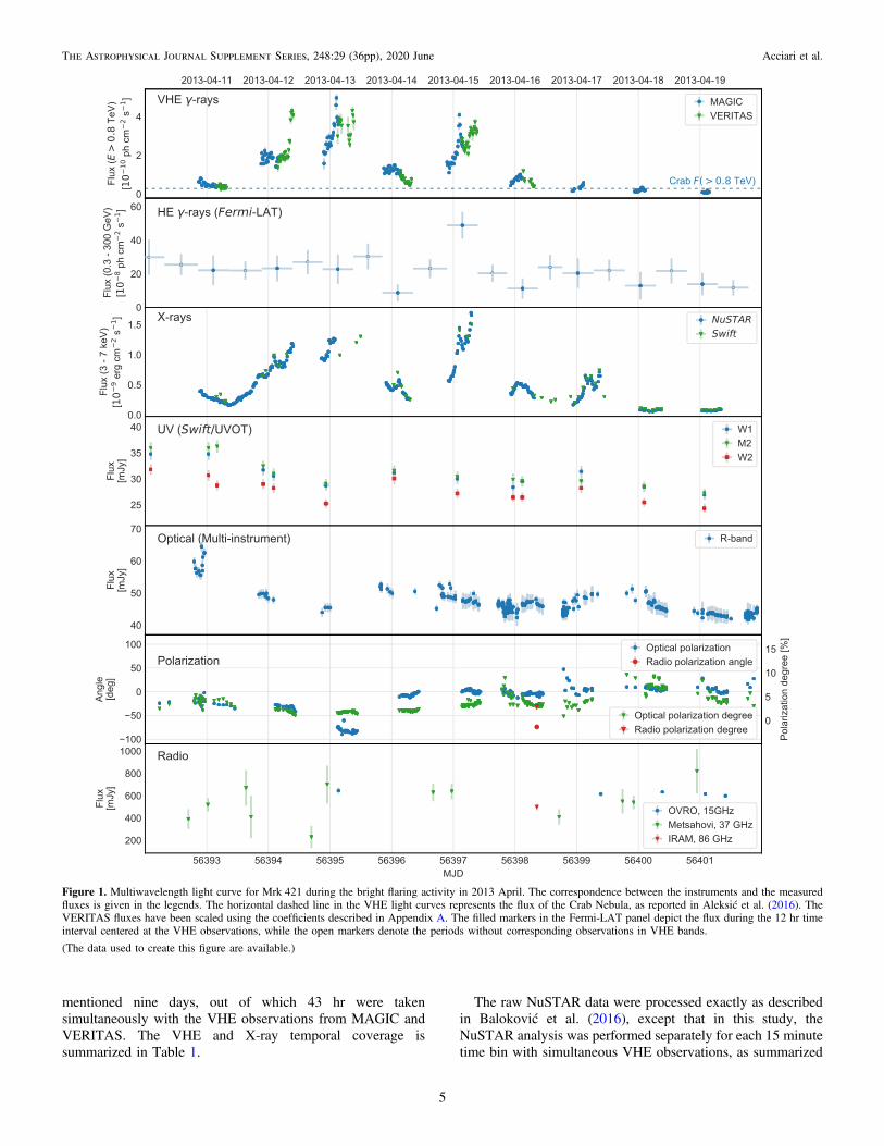
Figure 1. Multiwavelength light curve for Mrk 421 during the bright flaring activity in 2013 April. The correspondence between the instruments and the measuredfluxes is given in the legends. The horizontal dashed line in the VHE light curves represents the flux of the Crab Nebula, as reported in Aleksić et al. (2016). TheVERITAS fluxes have been scaled using the coefficients described in Appendix A. The filled markers in the Fermi-LAT panel depict the flux during the 12 hr timeinterval centered at the VHE observations, while the open markers denote the periods without corresponding observations in VHE bands.

(The data used to create this figure are available.)

5

The Astrophysical Journal Supplement Series, 248:29 (36pp), 2020 June Acciari et al.

in Table 1. Using Xspec (Arnaud 1996), we calculated fluxes inthe 3–7keV, 7–30keV, and 30–80keV bands from a fit of alog-parabolic model to the data within each time bin. Thecross-normalization between the two NuSTAR telescopemodules was treated as a free parameter. The statisticaluncertainties of the fluxes were calculated at 68% confidenceintervals and do not include the systematic uncertainty in theabsolute calibration, which is estimated to be 10%–20%(Madsen et al. 2015).

The analysis procedures used to process the Swift-XRT dataare described in Baloković et al. (2016). In addition, in order toavoid additional flux uncertainties, we excluded 16 Swift-XRTobservations in which Mrk 421 was positioned near the CCDbad columns (Madsen et al. 2017). Figure 1 shows acomparison of the Swift-XRT and NuSTAR X-ray fluxes inthe band 3–7keV. Overall, there is a good agreement betweenthe two instruments, with flux differences typically smaller than20%. Such flux differences are within the systematicuncertainties in the absolute flux calibration of NuSTAR(Madsen et al. 2015) and Swift-XRT (Madsen et al. 2017).

Differently to the Fermi-LAT analysis reported in Balokovićet al. (2016), the LAT data results shown here were producedwith events above 0.3GeV (instead of 0.1 GeV) and with Pass8(instead of Pass7). The analysis above 0.3GeV is less affected bysystematic uncertainties, and it is also less sensitive to possiblecontamination from non-accounted (transient) neighboringsources. The higher minimum energy somewhat reduces thedetected number of photons from the source, but, owing to itshard gamma-ray spectrum (photon index <2.0), the effect issmall. Specifically, we used the standard Fermi analysis softwaretools version v11r07p00, and the P8R3_SOURCE_V2 responsefunction on events with energy above 0.3GeV coming from a10° region of interest (ROI) around Mrk 421. We used a 100°zenith-angle cut to avoid contamination from the Earth’s limb,67

and we modeled the diffuse Galactic and isotropic extragalacticbackground with the files gll_iem_v07.fits and iso_P8R3_SOURCE_V2_v1.txt, respectively.68 All point sources in thefourth Fermi-LAT source catalog (4FGL; Abdollahi et al.2020) located in the 10° ROI and an additional surrounding 5°-wide annulus were included in the model. In the unbinnedlikelihood fit, the spectral parameters were set to the valuesfrom the 4FGL, while the normalization of the diffusecomponents and the normalization parameters of the 16sources (within the ROI) identified as variable were initiallyleft free to vary. However, owing to the short timescalesconsidered in this analysis, only two of these sources weresignificantly detected in 10 days: 4FGLJ1127.8+3618 and4FGLJ1139.0+4033, and hence, we fixed the normalization ofthe other ones to the 4FGL catalog values. The Fermi-LATspectrum from the 10 day time period considered here (fromMJD 56392 to MJD 56402) is well described by a power-lawfunction with a photon flux above 0.3GeV of (23.3± 1.6)×10−8 cm−2 s−1 and photon index 1.79±0.05. A spectralanalysis over 1 day and 12 hr time intervals shows that thephoton index does not vary significantly throughout the 10 dayperiod. The data was split into 12 hr–long intervals centered atthe VHE observations (e.g., simultaneous to the VHE) and theircomplementary time intervals (e.g., when there are no VHE

observations), which are close to 12 hr–long intervals. Owingto the limited event count in the 12 hr time intervals and thelack of spectral variability throughout the 10 day period, wefixed the shape to a power-law index of 1.79 (the value fromthe 10 day period) to derive the photon fluxes, always keepingthe normalization factor for Mrk 421 and the two above-mentioned 4FGL sources as free parameters in the log-likelihood fit of each of the 12 hr time intervals.The characterization of the activity of Mrk 421 at optical

frequencies was performed with many instruments from theGLAST-AGILE Support Program (GASP) of the Whole EarthBlazar Telescope (WEBT), hereafter GASP-WEBT (e.g.,Villata et al. 2008, 2009), namely, the observatory in Roquede los Muchachos (KVA telescope), Lowell (Perkins tele-scope), Crimean, St. Petersburg, Abastumani, Rozhen (50/70 cm, 60 cm, and 200 cm telescopes), Vidojevica, and Lulin.Moreover, this study also uses data from the iTelescopes, theRemote Observatory for Variable Object Research (ROVOR),and the TUBITAK National Observatory (TUG). The polariza-tion measurements were performed with four observatories:Lowell (Perkins telescope), St. Petersburg, Crimean, andSteward (Bok telescope). The data reduction was done exactlyas in Baloković et al. (2016).Other than the 15 and 37GHz radio observations performed

with the OVRO and Metsahovi telescopes, which were describedin Baloković et al. (2016), here, we also present a fluxmeasurement performed with the IRAM30m telescope at86GHz. This observation was performed under the PolarimetricMonitoring of AGNs at Millimeter Wavelengths program(POLAMI,69 Agudo et al. 2018b), which regularly monitorsMrk 421 in the short millimeter range. The POLAMI data wasreduced and calibrated as described in Agudo et al. (2018a).

3. Multi-instrument Light Curves during the OutstandingFlaring Activity in 2013 April

The multi-instrument light curves derived from all of theobservations spanning from radio to VHE gamma-rays are shownin Figure 1. The top panel of Figure 1 shows an excellentcoverage of the nine day flaring activity in the VHE regime as aresult of the combined MAGIC and VERITAS observations. Thepeak flux at TeV energies, observed on April 13 (MJD 56395),reached up to 15 times the flux of the Crab Nebula, which is about30 times the typical non-flaring activity of Mrk 421 and about 150times the activity shown a few months before, on 2013 Januaryand February, as reported in Baloković et al. (2016). Moreover,this is the highest TeV flux ever measured with MAGIC for anyblazar. This is also the third highest flux ever measured from ablazar with an IACT, after the extremely large outburst fromMrk 421 detected with VERITAS in 2010 February (Abeysekaraet al. 2020) and the large flare from PKS2155-304 detected byHESS in 2006 July (Aharonian et al. 2007).Figure 1 shows that the most extreme flux variations occur in

the X-ray and VHE gamma-ray bands. At GeV energies, withinthe accuracy of the measurements, there is enhanced activityonly for MJD56397 (April 15), when the flux is about a factorof two larger than the flux in the previous and in the following∼12 hr time intervals. Interestingly, on April 15, we also findthe highest X-ray flux and the highest intra-night X-ray fluxincrease measured during this flaring activity in 2013 April.

67 A zenith-angle cut of 90° is needed if using events down to 0.1GeV, butone can use a zenith-angle cut of 100° above 0.3GeV without the need forusing a dedicated Earth limb template.68 https://fermi.gsfc.nasa.gov/ssc/data/access/lat/BackgroundModels.html 69 http://polami.iaa.es

6

The Astrophysical Journal Supplement Series, 248:29 (36pp), 2020 June Acciari et al.

The R-band activity is comparable to the one measured in 2013January–March, when Mrk 421 showed very low VHE and X-rayactivity (Baloković et al. 2016). The measured fluxes at opticalwavelengths are large when compared to the flux levels typicallyseen during the period of 2007–2015 (Carnerero et al. 2017).Generally, during the observations performed in 2013 January–April, Mrk 421 was four to five times brighter in the optical thanwere the photometric minima that occurred in 2008–09 and at theend of 2011. Figure 1 shows that Mrk 421 faded at the R bandfrom about 60mJy on MJD56393 to about 45mJy two dayslater. It then varied between 45 and 50mJy during the followingweek and appeared decoupled from the VHE and X-ray activity.The optical light curve is in agreement with that of the lesswell-sampled Swift/UVOT light curve. Other than the opticalbrightness of Mrk 421 in 2013, the object showed a bluer opticalcontinuum than average. This was determined from the differentialspectrophotometry obtained by the Steward Observatory monitor-ing program. By comparing the instrumental spectrum of Mrk 421with that of a nearby field comparison star, it is found that forthe wavelengths 475 and 725nm that [F(475)/F(725)]2013 April/[F(475)/F(725)]average=1.072± 0.002, where the averageinstrumental flux ratio is determined from all of the availableobservations from 2008 to 2018. The bluer color of Mrk 421 isconsistent with a higher dominance of the nonthermal continuumover the host galaxy starlight included within the observingaperture, which has a redder spectrum. This explanation for theobserved variations in the optical color of Mrk 421 is furtherconfirmed by the trend that the continuum becomes slightlyredder, as the AGN generally fades during 2013 April. The sametrend in color is also seen in the long-term near-IR data (Carnereroet al. 2017).

The optical linear polarization of Mrk 421 was also monitored,and the measurements are shown in Figure 1. Again, the resultsare comparable to those measured during the first quarter in 2013and reported in Baloković et al. (2016). Since 2008, the degree ofpolarization, P, has ranged from 0% to 15%; although,observations of P > 10% are rare, about 10 out of around1400 observations (Carnerero et al. 2017). During 2013 April, thepolarization ranged from about 1%–9%, with a large majority ofmeasurements showing P < 5%. The largest changes in thedegree of polarization on a daily timescale were an increase fromP∼3% to P∼7% on MJD56399/400, followed by a decreaseback to about 4% on the next day. Changes of nearly as much as5% in polarization are observed within a day, particularly forMJD56398/99, but otherwise, variations in P are typicallylimited to <1% over hour timescales. The electric vector positionangle (EVPA) of the optical polarization was at about −20° at thestart of 2013 April. Between MJD56394 and MJD56395, theEVPA rotated from about −30° to about −90° while, generally,P < 2.5%. The largest daily rotation in EVPA occurs betweenMJD56395 and MJD56396, where the EVPA goes from about−90° to about −10° . Because of the daily gap in the opticalmonitoring, it is unfortunately not clear if the EVPA reversed itsdirection of rotation from MJD56394 to MJD56396 (i.e., 2days) or continued in the same direction requiring a rotation>90°during one of the two observing gaps for MJD56394/6. Thevariability of Mrk 421 during the densely sampled portions of theoptical monitoring does not hint that such large changes in EVPAcan take place on short timescales until near the the end ofMJD56398 when a counterclockwise rotation of about 50° isseen over a period of about 6 hr. Outside of this excursion, theEVPA stays near 0° from MJD56396 onward. The single daily

deviation of the EVPA to 90°–100° for MJD56395 coincideswith brightest VHE flare observed in 2013 April. However, nosignificant change in the EVPA is apparent during the sharp risein VHE flux observed near the middle of MJD56394 or duringthe dramatic high-energy activity at the beginning of MJD56397.For most of the monitoring period, the optical EVPA was near thehistorically most likely angle for this object (EVPA=0°;Carnerero et al. 2017); although, the one-day excursion onMJD56395 brought the EVPA nearly orthogonal to the mostlikely value. For comparison, the 15 GHz VLBI maps of Mrk 421show a jet detected out to about 5 mas at a position angle of about−40° (Lister et al. 2019). In the radio band, the activity measuredduring the entire nine day observing period is constant, with aflux of about 0.6Jy. The single 86GHz measurement withIRAM30m shows a polarization degree of about 3%, which issimilar to that of the optical frequencies; yet, the polarizationangle differs by about 70°, which suggests that the optical andradio emissions are being produced in different locations of thejet of Mrk 421. Overall, the radio and optical fluxes, as well theoptical polarization variations (polarization degree and EVPA),appear completely decoupled from the large X-ray and VHEgamma-ray activity seen in 2013 April. In fact, the behaviorobserved at radio and optical during 2013 April is similar to thatobserved during the previous months, when Mrk 421 showedextremely low X-ray and VHE gamma-ray activity (seeBaloković et al. 2016).The hard X-ray and VHE gamma-ray bands covered with

NuSTAR, MAGIC, and VERITAS are the most interesting onesbecause they exhibit the largest flux variations and because of theexquisite temporal coverage and the simultaneity in the data set.Figure 2 reports the flux measurements in these bands, each splitinto three distinct bands, 3–7keV, 7–30keV, and 30–80keVfor70 NuSTAR and 0.2–0.4TeV, 0.4–0.8TeV, and >0.8TeVfor MAGIC and VERITAS. The temporal coverage for the>0.8 TeV band is a about 2 hr longer than for the 0.2–0.4 TeVband because of the increasing analysis energy threshold withthe increasing zenith angle of the observations. The exquisitecharacterization of the multiband flux variations in the X-rayand VHE gamma-ray bands reported in Figure 2 will be used inthe sections that follow for the broadband variability andcorrelation studies.

4. Multiband and Multi-timescale Variability

4.1. Fractional Variability

The flux variability reported in the multiband light curvescan be quantified using the fractional variability parameter Fvar,as prescribed in Vaughan et al. (2003):

( )s=

- á ñá ñg

FS

F. 2var

2err2

2

á ñgF denotes the average photon flux, S denotes the standard

deviation of N flux measurements, and sá ñerr2 denotes the mean

squared error, all determined for a given instrument and energyband. The uncertainty on Fvar is calculated using the prescriptionfrom Poutanen et al. (2008), as described in Aleksić et al. (2015a).This formalism allows one to quantify the variability amplitude,

70 The upper edge of the NuSTAR energy range is actually 79keV, but owingto the negligible impact on the flux values, in this paper, we will use 80keV forsimplicity.

7

The Astrophysical Journal Supplement Series, 248:29 (36pp), 2020 June Acciari et al.

with uncertainties dominated by the flux measurement errors andthe number of measurements performed. The systematicuncertainties on the absolute flux measurements71 do not directlyadd to the uncertainty in Fvar. The caveats in the usage of Fvar toquantify the variability in the flux measurements performed withdifferent instruments are described in Aleksić et al. (2014, 2015a,2015b). The most important caveat is that the ability to quantifythe variability depends on the temporal coverage (observingsampling) and the sensitivity of the instruments used, which aresomewhat different across the electromagnetic spectrum. A bigadvantage of the study presented here is that the temporalcoverage of the three bands in X-rays (from NuSTAR) and thethree bands in VHE gamma-rays (from MAGIC and VERITAS)is exactly the same, which allows us to make a more directcomparison of the variability in these energy bands.

The fractional variability parameter Fvar was computed usingthe flux values and uncertainties reported in the light curves fromSection 3 (see Figures 1 and 2), hence, providing a quantificationof variability amplitude for this nine day–long flaring activityfrom radio to VHE gamma-ray energies. The results are depictedin the upper panel of Figure 3, where open markers are used forthe variability computed with all of the available data, and filledmarkers are used for simultaneous observations. Given theslightly different temporal coverage for the different VHE bands,as described in the previous section, we decided to use the0.2–0.4TeV band to define the time slots for simultaneous

X-ray/VHE observations. This ensures that the same temporalbins are being used for the 3×3 X-ray and VHE bands. Forcomparison purposes, we added the Fvar values obtained for theperiod from 2013 January to March, when Mrk 421 showed verylow activity (see Baloković et al. 2016).The fractional variability plot shows the typical double-

bump structure, which is analogous to the broadband SED.This plot shows that most of the flux variations occur in theX-ray and VHE bands, which correspond to the fallingsegments of the SED. Additionally, it also shows that, duringthe nine day flaring activity in 2013 April, the amplitudevariability in the hard X-ray band was substantially larger thanthat measured during the low activity from 2013 January toMarch. The higher the X-ray energy, the larger the differencebetween the Fvar values from the low and the high activity.In addition to the study of the nine day behavior, the high

photon fluxes and the deep exposures allow us to compute Fvar

with the single-night light curves from six consecutive nights(from April 11 to 17),72 hence, allowing us to study thefractional variability on hour timescales for the three X-raybands and three VHE gamma-ray bands. For this study, onlysimultaneous data (using the time bins from the 0.2–0.4 TeVband) were used, which means that the 3×3 X-ray/VHEbands sample exactly the same source activity. The results aredepicted in the lower panels of Figure 3. In general, all Fvar

values computed with the single-night light curves are lowerthan those derived with the nine day light curve for the

Figure 2. Light curves in various VHE and X-ray energy bands obtained with data from MAGIC, VERITAS, and NuSTAR (split in 15 minute time bins) and Swift-XRT (from several observations with an average duration of about 17 minutes). For the sake of clarity, the 0.3–3keV fluxes have been scaled by a factor 0.5. Thestatistical uncertainties are, in most cases, smaller than the size of the marker used to depict the VHE and X-ray fluxes.

(The data used to create this figure are available.)

71 The systematic uncertainties in the flux measurements at the radio, optical,X-ray, and GeV bands are of the order of 10%–15%, while those of the VHEbands are ∼20%–25%.

72 The light curves from April 18 and 19 contain little data (∼2 hr) and littlevariability, which prevents the calculation of significant (>3σ) variability formost of the energy bands.

8

The Astrophysical Journal Supplement Series, 248:29 (36pp), 2020 June Acciari et al.

corresponding energy band. This is clearly visible whencomparing the data points with the gray shaded regions inthe upper panel of Figure 3. Despite the X-ray and VHE fluxvarying on sub-hour timescales, the resulting intra-night

fractional variability is significantly lower than the overallfractional variability in the nine day time interval. This result isexpected because, while for single days, the light curves showflux variations within a factor of about two, the nine day light

Figure 3. Upper panel: fractional variability Fvar vs. energy band for the nine day interval from April 11–19. The panel reports the variability obtained using allavailable data (open symbols) and using only data that were taken simultaneously (filled symbols). For comparison, the Fvar vs. energy obtained with data from 2013January–March (see Baloković et al. 2016) is also depicted with gray markers. The gray shaded regions depict the range of Fvar obtained with data from single-nightlight curves, as shown in the lower panels. Lower panels: Fvar vs. energy for the three X-ray and VHE bands, using simultaneous observations and calculated for eachnight separately. In all plots, the vertical error bars depict the 1σ uncertainty, while the horizontal error bars indicate the energy range covered. In order to improve thevisibility of the data points, some markers have been slightly shifted horizontally (but always well within the horizontal bar).

(The data used to create this figure are available.)

9

The Astrophysical Journal Supplement Series, 248:29 (36pp), 2020 June Acciari et al.

curve shows flux variations larger than a factor of about 10.Unexpectedly, we find a large diversity in the variability versusenergy patterns observed for the different days. On April 13,15, 16, and 17, one finds a typical pattern of higher fractionalvariabilities at higher photon energies within each of the twoSED bumps. On the other hand, one finds that the fractionalvariability is approximately constant with energy on April 11and 14 and that the fractional variability decreases with energyon April 12. The decrease in Fvar with increasing energy is onlymarginally significant in the VHE bands (∼2σ) but veryprominent in the X-ray emission, within which the synchrotronself-Compton (SSC) scenario, provides a direct mapping to theenergy of the radiating electrons. These different variabilityversus energy patterns suggest the existence of diverse causes(or regions) responsible for the variability in the broadbandblazar emission on timescales as short as days and hours. Thisis the first time that the variability of Mrk 421 has been studiedwith this level of detail, and the implications will be discussedin Section 6.

4.2. Flux Variations on Multi-hour and Sub-hour Timescales

This section focuses on the flux variations observed in thehard X-ray and VHE gamma-ray bands, which are the oneswith the largest temporal coverage and highest variability (seeSection 4.1). The light curves for all nights for these 3× 3energy bands are reported in Appendix B. There is clear intra-night variability in all of the light curves, which can besignificantly detected because of the high fluxes and the goodtemporal coverage, as described in the previous section (e.g.,see Figure 3). The single-night light curves show a largediversity of temporal structures that relate to different time-scales, from sub-hours (i.e., fast variation) to multi-hours(trends). We note that some of these fast components arepresent in both X-rays and VHE gamma-rays, while someothers are visible only at X-rays or only at VHE gamma-rays,and, in some cases, the features are present only in specificbands (either X-rays or VHE gamma-rays) and not in theothers. As it occurred with the study of the Fvar versus energy,the evaluation of the single-night multiband light curves alsosuggests that there are different mechanisms responsible for thevariability, some of them being achromatic (affecting allenergies in a similar way) and others chromatic (affecting thedifferent energy bands in a substantially different manner).

In this section, we attempt to quantify the main trends andfast features, as well as their evolution across the variousenergy bands. We do that by fitting with a function formed by aslow trend Fs (t) and fast feature Ff (t) components.

( ) ( ) ( ) ( )= +F t F t F t 3s f

where

( ) · ( · ) ( )= +F t tOffset 1 Slope 4s

and

( ) · · ( ) ( )=+- - -F t A F t2

2 2. 5f s 0t t

tt tt

0rise

0fall

Here, A is the flare amplitude, t is the time since midnight forthe chosen night, t0 is the time of the peak flux of the flare, andtrise and tfall are the flux-doubling timescales for the rising andfalling part of the flare, respectively. This formulation, with theslope of the slow component normalized to the offset, and the

flare amplitude (of the fast component) normalized to the slowcomponent at t0, enables a direct comparison of the parametervalues among the different energy bands, for which the overallmeasured flux may differ by factors of a few.In general, we find that, whenever fast flares occur, they

appear to be quite symmetric and, given the relatively shortduration (sub-hour timescales) and the flux measurementuncertainties, we do not have the ability to distinguish (in astatistically meaningful way) between different rise- and fall-doubling times. For the sake of simplicity, we decided to fit thelight curves with a function given by Equation (5) wheretrise=tfall=flux-doubling time. This fit function provides afair representation of the intra-night rapid flux variations fromall days except for April 16, where the flux variations havemuch longer (multi-hour) timescales.This relatively simple function provides a rough description

of the energy-dependent light curves and may not describe allof the data points perfectly well. For instance, in the low-energy X-ray bands, the statistical uncertainties are very small,and one can appreciate the significant and complex substructurethat is not reproduced by the above-described (and relativelysimple) fitting function. We do not intend to find a model thatdescribes all of the data points accurately. Rather, we look for amodel that provides a description of the main flux-variabilitytrends and how they evolve with the X-ray and VHE energies.The multiband flux variations during April 15 and its related

quantification using Equation (3) are depicted in Figure 4, withthe parameters resulting from the fits reported in Table 2. Themain multiband emission varies on timescales of several hours,and hence, it is dominated by the “slow component” inEquation (3). The slope of this variation (quantified relative tothe offset in each band for better comparison among all bands)has a strong energy dependence, with the parameter value for thehighest energies being around a factor of two to three times largerthan that for the lowest energies for both the X-ray and VHEgamma-ray bands (e.g., Slope>0.8 TeV ; 3·Slope0.2–0.4 TeV). Thesecond most important feature of this multiband light curve is theexistence of a short flare, on the top of the slowly varying flux, inall of the energy bands for both X-rays and VHE gamma-rays.The location of the flare t0 is the same (within uncertainties) in allthree X-ray bands and VHE bands. In order to better quantify thelocation of the short flare at the X-ray and VHE gamma-rayenergies, using the information from Table 2, we computed theweighted average separately for the three VHE bands,t0, VHE=2.44±0.03 hr and the three X-ray bands,t0, X-ray=2.41±0.04 hr past midnight. This indicates that, forthis fast feature in the light curve, for all of the energies probed,there is no delay in between the X-ray and VHE gamma-rayemissions down to the resolution of the measurement, which,adding the errors in quadrature, corresponds to 3 minutes. Theflux-doubling time is comparable among all of the energy bands,with about 0.3 hr for all of the X-ray bands and the highest VHEband (>0.8 TeV), and about 0.2 hr for the lowest and middleVHE bands. The characteristic by which the fast X-ray flarediffers from the fast VHE flare is in the normalized flareamplitude A (see Table 2): it is energy independent (achromatic)for the X-ray fast flare, while it increases its value (chromatic) forthe VHE fast flare (with amplitude A>0.8 TeV ; 2·A0.2–0.4 TeV).In order to evaluate potential spectral variability throughout the

∼10 hr light curves measured on 2013 April 15, we computed theflux hardness ratios HR (=Fhigh-energy/Flow-energy) for several

10

The Astrophysical Journal Supplement Series, 248:29 (36pp), 2020 June Acciari et al.

energy bands in both the X-ray and VHE gamma-ray domains.Figure 5 depicts the HR computed with the data fluxmeasurements (in time bins of 15 minutes) and the HR expectedfrom the fitted functions reported in Figure 4 and Table 2. Forcomparison purposes, we also included the HR from the fittedfunctions from Table 2 excluding the fast component given byEquation (5) (dotted line in Figure 5). The dashed vertical red lineindicates the weighted average time of the peak of the flare t0,calculated separately for the three X-ray bands and VHE gamma-ray bands (see above). One can see that the overall impact of thefast component in the HR temporal evolution is small and onlynoticeable in some panels (e.g., F>0.8 TeV/F0.4–0.2 TeV orF7–30 keV/F3–7 keV). This is due to the relatively short durationof the fast component and the relatively small magnitude of theflare amplitude, in comparison to the overall flux. Therefore, thetemporal evolution of the spectral shape in both bands, X-ray andVHE, is dominated by the slow component, i.e., by the variationswith timescales of several hours.

In addition to April 15, we also performed the fit withEquation (3) to the other five consecutive nights with largeX-ray and VHE gamma-ray simultaneous data sets, namely allnights from April 11 to 16 (both included). The results fromthese fits are reported in Appendix C (see Table C1 andFigures C1–C5). It is worth stating that, when comparing thequantification of the various light curves with the function inEquation (3), we found diversity among the fit parametervalues and their energy dependencies. For April 11, we did notfind any fast component, and the flux decreases monotonicallythrough the observation with energy-independent slope forboth the X-rays and VHE gamma-rays (fully achromatic fluxvariations). On the other hand, during April 12, the emissionincreased throughout the observation but with a slope that

decreased with increasing energy in both the X-rays and VHEgamma-rays. This trend is also observed, from a differentperspective, in the lower-right panel of Figure 3, whichdisplays a decreasing Fvar with increasing energy for both theX-ray and VHE gamma-ray emissions from April 12. This is avery interesting behavior because it is opposite to the trendreported in most data sets from Mrk 421, where the variabilityincreases with energy. For this night, we can also see a fastX-ray flare (flux-doubling time of about 0.3 hr) whoseamplitude increases with energy. Unfortunately, this fastX-ray flare occurred during a time window without VHEobservations.For April 13, we also observed a slow flux variation with an

energy-independent slope, as on April 11, but this time with aflux increase instead of a decrease. Additionally, we didobserve a super-fast X-ray flare (flux-doubling time of 5± 1minutes) without any counterpart in the VHE light curve, i.e.,an “orphan” X-ray flare (see Figure C3). As shown inTable C1, the X-ray NusTAR flare amplitude relative to theoverall baseline is only about 11%, but it is significant (3–4σdepending on the energy band), and there is no correlated fluxvariation in the simultaneous VHE MAGIC fluxes, which haveflux uncertainties of about 5%.On April 14, we see again a monotonically decreasing flux

with an energy-independent slope for both the X-rays and VHEgamma-rays, with another fast X-ray flare (flux-doublingtime∼0.5 hr) without a counterpart in the VHE light curve.The night that differs the most is April 16, which does not

show any monotonic increase or decrease and shows a largelynonsymmetric flare with flux variation timescales of hours. Inorder to quantify the temporal multiband evolution of the fluxduring April 16, we used Equation (5) (i.e., the fitting function

Figure 4. Light curves from 2013 April 15 in the three X-ray bands (left panel) and three VHE gamma-ray bands (right panel). The red curve is the result of a fit withthe function in Equation (3), applied to the time interval with simultaneous X-ray and VHE observations. The resulting model parameters from the fit are reported inTable 2.

(The data used to create this figure are available.)

11

The Astrophysical Journal Supplement Series, 248:29 (36pp), 2020 June Acciari et al.

without the slow component), with ¹t trise fall. See Appendix Cfor further details about the quantification of the multiband fluxvariations during the six consecutive nights, from April 11to 16.

In summary, during these six consecutive nights withenhanced activity and with multi-hour-long X-ray/VHEsimultaneous exposures in 2013 April, we found achromaticand chromatic flux variability, with timescales spanning frommulti-hours to sub-hours, and several X-ray fast flares withoutVHE gamma-ray counterparts. We did not see any VHEgamma-ray orphan fast flares (whenever we had simultaneousX-ray coverage). However, we did observe fast flares in somespecific energy bands that are not detected in the other nearbyenergy bands (X-ray or VHE), which suggests the presence offlaring mechanisms affecting relatively narrow energy bands.

The temporal evolution of the X-ray and VHE emissions,and the particularity of being able to approximately describe itwith a two-component function with a fast (sub-hour variabilitytimescale) and slow (multi-hour variability), will be discussedin Section 6.

5. Unprecedented Study of the Multiband X-Ray and VHEGamma-Ray Correlations

We evaluated the correlations among all of the frequenciescovered during the 2013 April flare and found that the largest fluxvariations and the largest degree of flux correlation occurs in theX-ray and VHE gamma-ray bands. No correlation was foundamong the radio, optical, and gamma-ray bands, a result that wasexpected because of the lower activity and longer variabilitytimescales at these energies. Apart from some variability in theGeV flux around April 15, which is the day with the highestX-ray activity, the GeV emission appears constant for the 12 hrtime intervals related to flux variations by factors of a few at keVand TeV energies. If the GeV and TeV fluxes were correlated on12 hr timescales, Fermi-LAT should have detected large fluxvariations, and hence, we can exclude this correlation.

The quality and extent of this data set, both in time and energy,allows for an X-ray/VHE correlation study that is unprecedentedamong all data sets collected from Mrk 421 and any other TeVblazar. The relation between the VHE gamma-ray and the X-rayfluxes in the 3×3 energy bands is shown in Figure 6 for the nineday flaring activity and in Figure 7 for April 15. The discretecorrelation function (DCF) and Pearson correlation coefficients, aswell as the slope of the VHE versus X-ray flux, are reported inTable 3. There is a clear pattern: the strength of the correlation

increases for higher VHE bands and lower X-ray bands. Thestrongest correlation is observed between the 3–7 keV and >0.8TeV bands. This combination of bands also shows a slope (fromthe fit in Table 3) closest to 1, among all of the 3×3 bandsreported. Moreover, the scatter in the plots becomes smaller as weincrease the VHE band and decrease the X-ray energy band. Thesmallest scatter, which can be quantified with the χ2 of the fit(lower values of χ2 relate to a smaller scatter in the data points),occurs for the combination >0.8TeV and 3–7keV.Figure 6 reveals that the different days occupy (roughly)

different regions in the VHE versus X-ray flux plots (for all ofthe 3×3 bands). This is expected because the largest fluxchanges occur on day-long timescales. In addition, individualdays appear to show different patterns. In order to bettercharacterize these different patterns (observed for the differentdays), we also computed the same quantities (DCF, Pearson,and linear fit) to the simultaneous data points from the singlenights with multi-hour light curves (namely, April 11–16). Theresults are reported in Table D1, in Appendix D.The main conclusions from this study performed on data

from April 11 to 16 are as follows73:

1. During some nights, namely on April 15 and 16, Mrk 421shows the “general trend” that is observed for the fullnine day flaring activity, with the highest magnitude andsignificance in the correlation occurring for the >0.8TeVversus the 3–7keV bands.

2. During other nights, namely on April 11, 13, and 14, thegeneral trend from the nine day data set is less visible: thereis a larger similarity in the magnitude and significance of thecorrelation among the various energy bands.

3. During one night, April 12, we found no correlation betweenthe X-ray and VHE gamma-ray bands, despite the significantvariability in both bands. The lack of correlation between theX-rays and VHE gamma-rays (being both highly variableand characterized with simultaneous observations) has notbeen observed to date in Mrk 421; although, it has beenobserved in another HBL (PKS 2155-304, from 2008August–September; Aharonian et al. 2009).

The correlation study was also performed splitting the dataset into two subsets: (a) April 15, 16, and 17 (which appearsomewhat away from the main trend in Figure 6), and (b) April

Table 2Parameters Resulting from the Fit with Equation (3) to the X-Ray and VHE Multiband Light Curves from 2013 April 15

Band Offseta Slope Flare Flare Flare χ2/d.o.f.(hr−1) Amplitude A Flux-doubling Timeb (hr) t0 (hr)

2013 Apr 15

3–7 keV 0.71±0.01 0.153±0.006 0.49±0.07 0.30±0.04 2.35±0.06 836/247–30 keV 0.78±0.02 0.199±0.009 0.59±0.11 0.30±0.04 2.41±0.06 889/2430–80 keV 0.21±0.01 0.241±0.018 0.56±0.18 0.32±0.09 2.50±0.10 111/240.2–0.4 TeV 6.60±0.17 0.031±0.008 0.40±0.09 0.23±0.07 2.41±0.09 96.9/380.4–0.8 TeV 2.99±0.07 0.042±0.008 0.72±0.09 0.19±0.03 2.47±0.04 68.1/42>0.8 TeV 1.68±0.05 0.103±0.010 0.82±0.08 0.27±0.03 2.41±0.04 90.0/45

Notes.a For VHE bands in 10−10 ph cm−2s−1, for X-ray bands in 10−9 erg cm−2 s−1.b Parameters trise and tfall in Equation (3) are set to be equal and correspond to the values of flare flux-doubling time.

73 On the nights of April 17–19, both the level of activity of Mrk 421 and theamount of data collected were substantially smaller, which prevents us frommaking detailed studies of the multiband correlations.

12

The Astrophysical Journal Supplement Series, 248:29 (36pp), 2020 June Acciari et al.

11, 12, 13, 14, 18, and 19. In comparison to the nine day dataset, the separate analysis of the two subsets yields a reductionof the scatter of the flux points around the main trends (whichshow up as a noticeable reduction in the χ2 values from the fit)and also a smaller dependence of the magnitude andsignificance of the correlations on the specific combination ofVHE and X-ray energy bands. The largest linear fit slopeoccurs for the combination >0.8TeV and 3–7keV in bothsubsets (as with the nine day data set), but while for subset (a)we continue having the largest significance and magnitude ofthe correlation for >0.8TeV and 3–7keV, in subset (b), thechange in magnitude and correlation with energy bands ismuch smaller, and the highest values occur for >0.8TeV and7–30keV. This indicates a somewhat different physical state ofthe source during those three consecutive days (April 15, 16,and 17) with respect to the others.

In addition to the VHE gamma-ray and the X-ray fluxes inthe 3×3 energy bands for April 15, Figure 7 also depicts theflux–flux values from the fitted functions reported inSection 4.2. This figure shows that multiple components inthe flux evolution (e.g., the fast component on the top of theslow component) appear as “different trends” in the flux–fluxplots with the flaring component having a sharper VHE fluxrise (with increasing X-ray flux) than the slow component.Because of the statistical uncertainties in the flux measure-ments, as well as the fact that one component has a muchsmaller flux and shorter duration, even for very good data setssuch as this one, it is not easy to recognize and separate thecontribution of different components in the flux–flux plots.However, these different patterns can produce collectivedeviations (when considering many of these different single-trends) that are statistically significant when fitting the data

points in the flux–flux plots with simple trends, such as thelinear or quadratic functions in the log–log scale.A discussion of these observational results is given in

Section 6.

6. Discussion of the Results

Although detailed SED and light-curve modeling are beyondthe scope of this paper, we discuss the main results of ouranalysis and provide possible interpretations.

6.1. Minimum Doppler Factor

In general, VHE gamma-rays can interact with low-energysynchrotron photons in order to produce electron-positronpairs. If both VHE gamma-ray and low-energy photons areproduced in the same region, then the criterion that thisattenuation is avoided so that the VHE gamma-rays may escapefrom the source and be detected leads to a lower limit on theDoppler factor (Dondi & Ghisellini 1995; Tavecchio et al.1998; Finke et al. 2008). Owing to the detection of 10 TeVphotons from Mrk 421 during this flaring activity, the relevantobserved synchrotron frequency for their attenuation is close to6×1012 Hz. In the R band (ν∼4.5×1014 Hz), the observedflux is close to 50mJy on 2013 April 15. Using 12minutes asthe shortest variability timescale (see Table 2) and extrapolat-ing the R-band flux to 6×1012 Hz assuming the same spectralshape as that obtained from the long-term SED (i.e., photonindex ∼1.6; Abdo et al. 2011), one finds δ35, which lies atthe high end of the values derived from the SED modeling ofFermi-LAT detected blazars (Ghisellini et al. 2010; Tavecchioet al. 2010; Paliya et al. 2017). The derived lower limit can berelaxed if the gamma-ray and optical emitting regions are

Figure 5. The X-ray hardness (flux) ratios for several X-ray (NuSTAR) bands (left panel) and VHE (MAGIC+VERITAS) bands (right panel) for April 15. In bothpanels, the dashed red vertical line indicates the average time of the peak of the flare in VHE = t 2.44 0.03 hr0,VHE , and X-rays ‐ = t 2.41 0.04 hr0,X ray , where theaverage is calculated for the three bands (Table 2). The solid gray curve shows the ratio of the fitted functions with parameters reported in Table 2, and the dashed grayline shows the ratio of the same fitted functions but for excluding the fast component.

(The data used to create this figure are available.)

13

The Astrophysical Journal Supplement Series, 248:29 (36pp), 2020 June Acciari et al.

decoupled, but the actual value would depend on the details ofthe theoretical model.

6.2. Flux–Flux Correlations

Flux–flux correlations have been the focus of many multi-wavelength campaigns during active and low states of blazaremission (for Mrk 421, see, e.g., Maraschi et al. 1999; Fossatiet al. 2008; Aleksić et al. 2015b), because their study maydifferentiate among emission models (see, e.g., Krawczynskiet al. 2002). Fossati et al. (2008), in particular, studied thecorrelations on a daily basis between TeV fluxes (E>0.4TeV) and X-ray fluxes, mostly in the 2–10keV band but alsoin the 2–4keV, 9–15keV, and 20–60keV bands. The work

we show here goes one step further, as it allows, for the firsttime, for the study of flux–flux correlations between multipleVHE gamma-ray and X-ray energy bands on a daily basis anddown to 15 minute time bins.The overall strong correlation found between the >0.8TeV

band and the lowest-energy X-ray band (3–7 keV; Figure 6 andTable D1) implies that the emissions are most likely co-spatialand produced by electrons with approximately the same energyvia synchrotron in X-rays and SSC processes in gamma-rays.In TeV blazars, like Mrk 421, the peak of the SSC spectrum istypically produced by inverse Compton scatterings in theKlein–Nishina regime (e.g., Tavecchio & Ghisellini 2016).The results presented in Section 5 reveal, however, a more

complicated picture, as the strong correlation mentioned above

Figure 6. VHE flux vs. X-ray flux in the three X-ray and three VHE energy bands. Data from all nine days are shown, with colors denoting fluxes from the differentdays. The gray dashed line is a fit with slope fixed to 1, and the black line is the best-fit line to the data, with the slope quoted in Table 3.

(The data used to create this figure are available.)

14

The Astrophysical Journal Supplement Series, 248:29 (36pp), 2020 June Acciari et al.

weakens or even disappears on certain days (e.g., 2013 April12). A weak correlation between X-rays and gamma-rays canbe produced if the emissions are produced by differentcomponents (e.g., Petropoulou 2014; Chen et al. 2016) or bydifferent particle populations, as in lepto-hadronic models(Mastichiadis et al. 2013). Different strengths of the correlationcan be predicted by adjusting the temporal variations of themodel parameters (e.g., injection rate of accelerated particles)and/or by having more than one emitting component in X-raysand gamma-rays.

The analysis presented in Section 5 also reveals that theslope of the correlation between the X-ray bands and thegamma-ray bands is generally sub-linear, i.e., µgF FX

m with

m1, and changes with time (Table D1). In the standard (one-zone) SSC scenario, a value m=2 is expected if only theelectron distribution normalization varies with time. Even inthis scenario though, different values of m can be obtainedwhen looking at correlations between different energy bands inX-rays and gamma-rays (Katarzyński et al. 2005). Moreover,values of m<2 are possible if several parameters change withtime (e.g., magnetic field strength and Doppler factor).Katarzyński et al. (2005) explored these flux–flux correlationsin detail with an SSC model for high-peaked BL Lac objectslike Mrk 421. They showed that m�1 is expected betweenenergy bands close to the peaks of the synchrotron and SSCcomponents, if the blob is expanding and the magnetic field is

Figure 7. VHE flux vs. X-ray flux in the three X-ray and three VHE energy bands for April 15. The black line is the track predicted by the Slow+Fast component fitfrom Equation (3). The lightness of symbols follows time: for MAGIC data, lightness decreases with time, and for VERITAS data, it increases in time, so that thecentral part of the night, where MAGIC and VERITAS observations overlap, is plot with darker symbols.

(The data used to create this figure are available.)

15

The Astrophysical Journal Supplement Series, 248:29 (36pp), 2020 June Acciari et al.

decreasing (see Figure 4 in Katarzyński et al. 2005).Petropoulou (2014) showed that, in a two-component SSCscenario, the slope of the correlation between 2–10keV and0.4–10TeV may vary strongly from m∼0 to ∼1 on day-longtimescales, with a pattern that depends on the varying modelparameter (i.e., injection rate or maximum electron energy). Aquadratic relation between X-rays and gamma-rays is alsoexpected in lepto-hadronic models, where the former act astargets for the photohadronic interactions of accelerated protonsthat result in the production of gamma-rays (Dimitrakoudiset al. 2012; Mastichiadis et al. 2013). A slope of m 1 can alsobe produced in proton synchrotron models, where variations inthe electron and proton injection rates are directly mapped tovariations in the X-ray and gamma-ray flux, respectively(Mastichiadis et al. 2013). The detailed modeling of the flux–flux correlations will be the topic of a future study.

6.3. Temporal Variability

One of the main results of this work is the detection of fast-evolving flares on top of a slower evolving emission in both theX-ray and VHE gamma-ray bands. Although this temporalbehavior was qualitatively discussed for some of the X-rayNuSTAR light curves in Paliya et al. (2015), here, we present aquantitative study of these characteristics in both the X-raylight curves and the VHE gamma-ray light curves (see Figure 4in Section 4.2 and Figures C1–C5 in Appendix C). In thefollowing paragraphs, we discuss possible interpretations forthe origin of the multiband temporal variability.

6.3.1. Acceleration and Cooling Processes

The rise and decay timescale of a flare may be associatedwith the acceleration and cooling timescales of the radiatingelectrons. In this case, one can use the fact that the accelerationand cooling timescales are found to be equal in order toestimate the magnetic field of the emitting region, as follows. Ifelectrons undergo Fermi-1 (or Fermi-2) acceleration, then theacceleration timescale, in the co-moving frame, can be written

as

( )p g¢ =¢

¢t

m c N

eB

26e a

acc

(e.g., Finke et al. 2008) where B′ is the tangled (co-moving)magnetic field strength, g¢ is the electron Lorentz factor in theco-moving frame, and Na�1 is the number of gyrations anelectron makes to double its energy. The synchrotron coolingtimescale is

( )ps g

¢ =¢ ¢

tm c

c B

6

4. 7e

syn

2

T2

Setting ¢ = ¢t tacc syn results in

( )s g

¢ =¢

Be

N

3

4. 8

aT2

The Lorentz factor of electrons producing the peak of the SSCmission can be estimated as

⎜ ⎟ ⎜ ⎟⎛⎝

⎞⎠

⎛⎝

⎞⎠ ( )g

dd¢ » » ´

-E

m c

E5 10

40 1 TeV9b

e

ssc2

41

ssc

where Essc is the observed energy of the peak of the SSCcomponent. Here, we use a value of δ consistent with the lowerlimit from gg pair production (Section 6.1). Here and from thispoint forward, we neglect factors of 1+z, which will be quitesmall given the redshift of Mrk 421 (z=0.03). To accelerateelectrons to this peak requires

⎜ ⎟ ⎜ ⎟⎛⎝

⎞⎠

⎛⎝

⎞⎠ ( )d

¢ »-

BN

940 100

G. 10a2 1

Large values of the magnetic field or large values of Na arerequired to accelerate electrons to g¢b where ¢ = ¢t tacc syn. Similarresults were found for the luminous, rapid flare from PKS 2155−304 in 2006 (Finke et al. 2008).Acceleration and cooling may control the light-curve

timescales, if ¢ ¢ = ¢R c t tb syn acc or ¢ ´R 1.4 10b12( )d -40 3

( )-N 100 cma2 , where ¢Rb is the radius of a spherical emitting

region in the co-moving frame. The required upper limit on¢Rb is two to three orders of magnitude smaller than typical

Table 3Correlation Coefficients and Slopes of the Linear Fit to the VHE vs. X-Ray Flux (in Log Scale) Derived with the Nine Day Flaring Episode of Mrk 421 in 2013 April

VHE Band X-Ray Band Pearson Coeff.a Nσ Pearsona DCF Linear Fit Slope χ2/d.o.f.

0.2–0.4 TeV 3–7 keV 0.92±0.01 20.2 0.93±0.12 0.61±0.02 1183/1627–30 keV 0.87±0.02 17.0 0.88±0.11 0.45±0.03 1891/16230–80 keV 0.79±0.03 13.6 0.81±0.11 0.35±0.02 2277/162

0.4–0.8 TeV 3–7 keV -+0.946 0.0090.007 23.4 0.96±0.11 0.79±0.03 1038/170

7–30 keV 0.91±0.01 19.8 0.92±0.11 0.58±0.03 1725/17030–80 keV 0.84±0.02 15.8 0.86±0.11 0.45±0.03 2160/170

>0.8 TeV 3–7 keV -+0.964 0.0060.005 26.0 0.97±0.11 1.11±0.03 704/170

7–30 keV -+0.947 0.0080.007 23.5 0.96±0.11 0.81±0.03 1245/170

30–80 keV 0.89±0.02 18.6 0.91±0.10 0.61±0.03 1736/170

Note.a The Pearson correlation function 1σ errors and the significance of the correlation are calculated following Press et al. (2007).

16

The Astrophysical Journal Supplement Series, 248:29 (36pp), 2020 June Acciari et al.

values for the size of the emitting region (e.g., Abdo et al. 2011),even for flaring episodes (e.g., Aleksić et al. 2015b).Additionally, if the flare’s rise and decay times were dominatedby the acceleration and cooling timescales, one would expect theflaring timescales to be energy dependent; however, they seem tohave the same timescale across energy bands (see Table 2).Therefore, the timescales of the fast component of the light curveare likely controlled by the light-crossing time of a blob with afixed size. As a result, they should appear symmetric and withtimescales independent of the energy.

6.3.2. Plasmoids in Magnetic Reconnection

Magnetic reconnection is invoked as an efficient particleacceleration process in a variety of astrophysical sources ofnonthermal high-energy radiation, including AGN jets (Romanova& Lovelace 1992; Giannios et al. 2009, 2010; Giannios 2013). Ithas been proposed that plasmoids (i.e., blobs of magnetized plasmacontaining energetic particles) that are formed and accelerated inthe reconnection regions of jets can serve as high-energy emissionsites in both blazars and radio galaxies (Giannios et al. 2009; Sironiet al. 2015). Petropoulou et al. (2016, hereafter PGS16) presented asemi-analytic model of flares powered by plasmoids in areconnection layer, simplifying the results of detailed particle-in-cell (PIC) simulations (for a full numerical treatment, see Christieet al. 2019).

A single plasmoid produces a flare with a peak luminosity andflux-doubling timescale that depend on its size and Dopplerbeaming. A unique feature of this model is that the flux-doublingtimescale in the rising part of the flare is mostly determined by theacceleration of the plasmoid in the layer (i.e., by its bulk motion).As a result, similar rise timescales should be observed at differentenergy bands of a flare powered by a single plasmoid (achromaticbehavior). In contrast to the rising part of a flare, its decay is notconstrained by PIC simulations. By setting the decay timescale tobe approximately equal to the rise timescale of the fast flares, asobserved, one can infer the declining rate at which acceleratedparticles are injected in the plasmoid or the decay rate of themagnetic field after the plasmoid has left the layer (PGS16).

No strong spectral evolution is expected during a flare producedby a single plasmoid (PGS16; Christie et al. 2019). At any giventime though, an observer receives radiation from a large number ofplasmoids in the layer, having different sizes and Doppler factors.Those plasmoids that move with mildly relativistic speeds (in thejet frame) and have intermediate sizes (in terms of the layer’s size)can contribute and even dominate the overall emission. Thesuperposition of their emission could result in a slowly varying andmore luminous component of the light curve (Giannios 2013;Christie et al. 2019), which may exhibit spectral variations anddrive the fractional variability on longer timescales than the fastvarying component of the light curve (Christie et al. 2020).

Energetics and timescales—PGS16 provided simple for-mulae to estimate the flux-doubling timescale (t1/2) and peakluminosity (Lpk) of flares produced by individual plasmoids in areconnection layer (with half-length L′)74 of a blazar jet (for anillustration, see Figure 3 in Christie et al. 2019). The bolometricpeak flare luminosity can be written as

( )pb d= ¢ ¢L cw u

211pk,bol g f

2p,f4

e

where βg is the growth rate of a plasmoid, ¢wf and dp, f are,respectively, the plasmoid transverse size and the Dopplerfactor at the end of its lifetime (i.e., when it is being advectedfrom the layer or when it merges with another biggerplasmoid). The Doppler factor takes into account the relativisticmotion of the plasmoid in the layer and the relativistic motionof the layer itself (for a definition, see Equation (8) in PGS16).In the above equation, pv b¢ Gu f L c4e rec j

2j j

2, where Γj is thejet’s bulk Lorentz factor, βj∼1, Lj is the absolute power of atwo-sided jet, v q¢ = GL rec j j is the cross-sectional radius ofthe jet, òrec;0.15 is the reconnection rate, and frec;0.5 is thefraction of dissipated magnetic energy transferred to relativisticpairs (e.g., Sironi et al. 2015). The flux-doubling timescale canbe estimated as

˜( ˜ )

( )òb d»

¢

¢

tc

dw

w

112

w

w

1 2g p1 2

f

where δp is the plasmoid’s Doppler factor (see Equation (8)in PGS16), which evolves during the plasmoid lifetime as thisaccelerates in the layer. Here, ¢w1 2 is the size of the plasmoid atthe moment the flare luminosity reaches half of its peak value.For details about the derivation of Equations (11)–(12) andassumptions therein, we refer the reader to PGS16. The freeparameters of the model are: the plasma magnetization σ, theorientation of the layer with respect to the jet axis θ′, theobserver’s angle θobs, L′, Lj, and Γj.We apply the PGS16 model to the fast flaring activity

observed in Mrk 421. We use as an illustrative example theresults for 2013 April 15, where fast flares with similarflux-doubling timescales (Table 2) have been detected in allenergy bands (3–7 keV, 7–30 keV, 30–80 keV, 0.2–0.4 TeV,0.4–0.8 TeV, and > 0.8 TeV). Using the peak flux of the fastflare in each energy band, we estimate the peak bolometricluminosity of the fast flare. Given the similar rise timescales inall bands, we use their mean value as the observed t1/2 of thefast flare (see the black symbol in Figure 8).We consider a case with plasma magnetization σ=10.

Other than the microphysical parameters, which are bench-marked with PIC simulations of reconnection (see Table 1in PGS16), we adopt the following values for the freeparameters of the model: L′=4×1015 cm, Lj=2×1046 ergs−1, Γj=14, and ( ) q = G -2 2 .1jobs

1 . Using Equations (11)and (12), we can then estimate the peak flux and flux-doublingtimescale of flares produced by plasmoids with different sizes,as shown in Figure 8. We note that the curves showingdifferent orientations of the reconnecting layer do not dependmonotonically on θ′ due to the kinematics of plasmoids in thejet (for details, see PGS16). For the adopted parameter values,we find that a larger range of θ′ values results in fluxes andflux-doubling timescales that are compatible with the observedvalues. A choice of larger L′ would just shift the curveshorizontally to longer timescales, while an increase of Γj wouldshift the curves diagonally toward the upper-left corner of theplot (for scalings, see Equations (33)–(37) in PSG16). A higherσ value would have a similar effect as that of a higher Γj, as itwould result in stronger relativistic motions of the plasmoids inthe layer. The predicted peak flux depends strongly on theangle at shorter variability timescales, whereas it is almostindependent of the orientation of the layer at longer timescales.This merely reflects the fact that flares with longer timescales74 Primed quantities are measured in the jet’s rest frame.

17

The Astrophysical Journal Supplement Series, 248:29 (36pp), 2020 June Acciari et al.

are produced by the largest plasmoids in the layer that movewith nonrelativistic speeds in the jet frame. For theseplasmoids, the beaming of the radiation is basically determinedby θobs and Γj. On the contrary, flares with short durations areproduced by plasmoids that move relativistically in the jetframe and whose Doppler factor δp depends sensitively on bothangles θ′ and θobs.

Flux–flux correlations—Here, we examine the flux–fluxcorrelations predicted by the model for the fast and slowcomponents of a plasmoid-powered light curve. To do so, weadopt the results of Christie et al. (2019) and, in particular, thelight curves computed for a “vanilla” model75 of a BL Lac–likesource for σ=10 (BL10) with θ′=30° and θobs=0°. Thevalues for the angles correspond to the vanilla BL Lac model ofChristie et al. (2019). A choice of 2°.1 instead of 0° would haveno effect on the conclusions. We focus on a 4 hr–long segmentof the total light curve that displays a fast flare (with duration∼0.3 hr) emerging on top of a less variable component (seeinset plot in Figure 9). The fluxes computed in the 3–7 keV and>0.8 TeV energy bands during the selected time window aredisplayed in the main panel of Figure 9 (blue points). Thefluxes computed during the fast flare are highlighted for clarity(orange colored points). Although our vanilla model cannotexplain the details of the observed correlations shown inFigure 7, the predicted flux–flux correlations bear somesimilarities with the observed ones: a tight correlation with aslope close to 1 is produced by the slow component of the light

curve, whereas the fast flare leads to a looser correlation with asteeper slope.We note that the temporal resolution of our model light

curve is about 30s. The loop-like structure produced by thefast component would likely be missed in real data due to thecoarser sampling. For example, even with the 15 minutesampling used in this work, the loop would consist of just twodata points. Our results are also in agreement with those shownin Figure 7, where the loop is not evident in the real data butbecomes visible only when the fitted fluxes of the slow and fastcomponents are plotted.Caveats—We next discuss some caveats of the plasmoid-

dominated reconnection model. The fast component of theoptical light curve is predicted to be wider than the one seen inthe X-rays and VHE gamma-rays, due to the longer coolingtimescales of electrons radiating in the optical band. Never-theless, some degree of correlation between the optical andother high-energy bands is expected in this model. Unfortu-nately, this cannot be tested with our current data set becausewe do not have proper optical coverage around the peak timesof the fast (sub-hour) flares in the X-rays and VHE gamma-rays(see Figures 1 and 4, C2–C4). On longer (multi-hour)timescales, the observed optical flux appears to roughly followthe temporal trends in X-rays and VHE gamma-rays for somedays (e.g., April 13 and 17), while it appears to beanticorrelated for some other days (e.g., April 11, 12, 15, and18). Such variability patterns cannot be explained by the vanillamodel we described above. If magnetic reconnection can betriggered in different jet locations, then it is possible to have theformation of multiple layers in the jet with different properties(e.g., sizes, magnetizations, and orientations; Giannios et al.2009; Giannios & Uzdensky 2019). It is then possible that theobserved optical emission is dominated by a different layer(e.g., larger and with different orientation) than the one

Figure 9. VHE flux (>0.8 TeV) vs. X-ray flux (3–7 keV) of a plasmoid-powered light curve, computed for a “vanilla” model of a BL Lac source (seemodel BL10 in Christie et al. 2019). The fluxes are extracted from a 4 hr timewindow of the total light curve (see the purple line in the inset plot) and arenormalized to their time-averaged values. The loop-like structure in the flux–flux plot is produced during a fast flare of duration ∼0.3hr (see orange points).Lines with slopes 1 (dashed) and 0.5 (dotted) are overplotted to guide the eye.

Figure 8. Bolometric peak flux of flares produced by plasmoids of differentsizes as a function of the respective flux-doubling timescale for σ=10. Thecolored curves correspond to different orientations (see the inset color bar) ofthe reconnecting layer with respect to the jet axis (for an illustration, see Figure3 in Christie et al. 2019). The solid thick lines indicate that the plasmoidDoppler factor 35, thus, satisfying the γγ opacity constraint (see Section 6.1).The peak bolometric flux and flux-doubling time of the fast flare observed on2013 April 15 is also shown (black symbol). A choice of larger L′ would shiftthe curves horizontally to longer timescales, while an increase of Γj would shiftthe curves diagonally toward the upper-left corner of the plot.

75 Performing detailed radiative transfer calculations, as in Christie et al.(2019), for parameters similar to those in Figure 8, lies beyond the scope of thispaper.

18

The Astrophysical Journal Supplement Series, 248:29 (36pp), 2020 June Acciari et al.

producing the high-energy emissions (e.g., smaller and morealigned to the observer).

To fully account for all of the observed properties of theflares (i.e., absolute flux and spectra), one would have to adjustsome of the parameters entering the vanilla model, such as theproperties of the injected particle distribution within eachplasmoid (e.g., slope, and minimum and maximum Lorentzfactor). The vanilla model described above could be improvedthrough the inclusion of continuous slow acceleration ofparticles within plasmoids due to plasmoid compression(Petropoulou & Sironi 2018) and/or impulsive particleinjection with a harder energy spectrum during plasmoidmergers (Christie et al. 2019).PGS16 and Christie et al. (2019) developed a radiative

model based on the PIC simulations of Sironi et al. (2016).Although the radiative model takes into account the plasmoidkinematics and dynamics, it treats each plasmoid as ahomogeneous source. Thus, this model cannot be used topredict the polarization signatures of a reconnection event. Thisissue has been recently tackled in Zhang et al. (2018), wherethe polarized emission was computed directly from 2D PICsimulations of reconnection, demonstrating that the latter canproduce variable optical polarization. Due to the differentsimulation setups used in Sironi et al. (2016) and Zhang et al.(2018), it is not clear how the polarization results found in thelatter study can be applied to the plasmoid-dominated modeldiscussed here.

7. Summary and Conclusions

This manuscript presents results from an extensive multi-wavelength campaign in 2013 on the blazar Mrk 421, whichincluded, for the first time, highly sensitive hard X-rayobservations with NuSTAR. This study focuses on theexceptional flaring activity observed during nine consecutivedays, from April 11 to 19, and complements the resultsobtained with the low VHE gamma-ray activity from 2013January to March, which was reported in Baloković et al.(2016). The 2013 April flaring activity is the brightest detectedwith MAGIC to date and the second brightest observed inMrk 421 to date, after the 2010 February flaring activityreported in Abeysekara et al. (2020). More important than thebright blazar activity is the comprehensive multi-instrumentdata set collected during these nine days, which includes 42 hrwith MAGIC, 27 hr with VERITAS, 18 hr with Swift, and 71hr with NuSTAR, out of which 43 hr were taken simulta-neously with the VHE observations from MAGIC andVERITAS.

Using simultaneous MAGIC–VERITAS observations ofMrk 421 during this high activity, we noticed that the VHEgamma-ray flux values from VERITAS are systematicallylower than those from MAGIC throughout the flaring activity.The flux difference is energy dependent, about 10% in the0.2–0.4TeV band and about 30% in the >0.8TeV band.These differences are within the quoted systematic uncertain-ties from both instruments and are probably related to theabsolute energy reconstruction. In order to perform variabilityand correlation studies during single days, the VERITAS fluxvalues were scaled up to match those from MAGIC (seeAppendix A). The physics results reported in this manuscriptrelate to the variations in the VHE gamma-ray flux and itscorrelation to the X-ray flux and, hence, do not depend on theabsolute value of the VHE gamma-ray flux. The results

reported here would essentially be the same if we had scaleddown the MAGIC fluxes to match the VERITAS fluxes.Owing to the large fluxes and the unprecedented coverage

provided by the simultaneous NuSTAR and MAGIC/VER-ITAS observations during these nine consecutive days, thisdata set allowed us to evaluate the variability and correlationsover three X-ray bands (3–7 keV, 7–30 keV, and 30–80 keV)and three VHE gamma-ray bands (0.2–0.4 TeV, 0.4–0.8 TeV,and >0.8 TeV) on timescales of 15 minutes, producing themost detailed X-ray/VHE variability and correlation study ofMrk 421 to date. This study yielded a number of results, whichwe summarize as follows:

1. The fractional variability Fvar versus energy for the nineday flaring activity shows a similar pattern to that duringthe low X-ray and VHE gamma-ray activity fromBaloković et al. (2016). The Fvar versus energy shows adouble-bump structure with the highest variabilityoccurring in the X-ray and VHE gamma-ray bands,while the variability in the radio and optical bands is verylow. Additionally, we find that: (a) the Fvar values for thehighest X-ray and VHE energies during this nine dayflaring activity are much higher than those from the lowactivity reported in Baloković et al. (2016); (b) the Fvar

values obtained with data from the single nights are muchsmaller than those obtained with the nine day flaringactivity, indicating that the processes with timescaleslarger than a half day dominate the variability at X-rayand VHE over the processes that have timescales ofhours; and (c) Fvar typically increases with energy forsingle nights, in the same way as observed for multi-dayor multi-month timescales; however, we also find nightswhere Fvar does not increase (or even decreases) withenergy, hence, suggesting the existence of distinctmechanisms (or distinct particle populations and/orregions) responsible for the variability of Mrk 421.

2. There is significant variability in the optical emission, aswell as in the polarization degree and EVPA (seeFigure 1), but they are not correlated with the X-rayand VHE gamma-ray emissions. The optical polarizationvariations, while statistically significant, relate to a verylow polarization degree (typically less than 5%) andappear to be random and without any obvious coherentstructure. This is consistent with a multi-zone scenariosuch as the one proposed in Marscher (2014), where thesum of the polarization vectors from many zones wouldresult in a low level of polarization with randomfluctuations in both the polarization degree and theEVPA. At 86GHz, the polarization degree is also low(about 3%), as also happens with the optical data, but thepolarization angle differs by about 70°, which indicatesthat the radio and optical emissions are produced, or atleast dominated, by different regions along the jet ofMrk 421.

3. The flux variability measured at GeV is dominated by thelarge flux variation around April 15, which is the daywith the highest X-ray activity. Despite the lowersensitivity of Fermi-LAT, in comparison to that of theX-ray and VHE gamma-ray instruments, the GeV flux ofMrk 421 can be measured significantly on 12 hrtimescales, and it does not show the large flux variations(by factors of a few) that are reported for the X-ray andVHE gamma-ray energies. Therefore, this observation

19

The Astrophysical Journal Supplement Series, 248:29 (36pp), 2020 June Acciari et al.

indicates that, when considering timescales of days, thereis no correlation between the GeV band and the keV andTeV bands.

4. In contrast to the 2013 January–March results reported inBaloković et al. (2016), the light curves from the 2013April flaring activity show substantial intra-day varia-bility in both the X-ray and VHE gamma-ray bands.Moreover, one can clearly distinguish variability on sub-hour timescales on the top of flux variations occurring onmulti-hour timescales. The intra-night flux variationswere quantified with a function consisting of anexponential increase and decay ( fast component) on thetop of a monotonically increasing or decreasing flux(slow component). We found out that, within the X-rayand VHE gamma-ray bands, the parameters describingthe fast component do not depend on energy, while thosedescribing the slow component can depend strongly onthe energy. We also found out that the fast component issymmetric (rise time ∼decay time). This suggests that themechanisms that dominate the production of the sub-hourflux variability appear to be “achromatic”, while thoseresponsible for the production of the multi-hour fluxvariability can be “chromatic”, at least in some cases.

5. A lower limit to the Doppler factor of 35 was derived byrequiring that the emitting region producing the fastestVHE variability is optically thin to γγ pair production(see Section 6.1). This limit implicitly assumes that thelow-energy (optical/IR) and VHE gamma-ray photonsare produced in the same region. However, the multibandvariability and correlations derived with the nine day2013 April flaring activity indicate that these twoemissions likely originated in different regions, whichwould relax the derived lower limit.

6. Using the parameters from the fast component, we findthat there are no delays between the X-ray and VHEgamma-ray emissions down to the resolution of ourmeasurement (3 minutes during April 15). This is thestrongest constraint on the correlated behavior betweenthe X-rays and gamma-rays in Mrk 421 and among thestrongest constraints derived with TeV blazar datauntil now.

7. The correlation between VHE gamma-rays and X-rays ispositive (i.e., the VHE gamma-ray emission increaseswhen the X-ray emission increases); but there aremultiple flavors in the strength and characteristics of thiscorrelated behavior that change both across energy (evenfor nearby energy bands) and over time (on daytimescales). The strongest correlation occurs betweenthe lowest X-ray band (3–7 keV) and the highest VHEgamma-ray band (>0.8 TeV), where one finds anapproximately linear change in the VHE flux with theX-ray flux. On the other hand, the weakest correlationoccurs between the highest X-ray band (30–80 keV) andthe lowest VHE gamma-ray band (0.2–0.4 TeV), wherethe VHE flux changes with the X-ray flux with a slope of∼0.3 in log–log scale. This indicates that the particlepopulation dominating the emission in the 3–7keV and>0.8TeV bands are closely related, while this does notoccur for the bands 30–80keV and 0.2–0.4TeV. Thedecrease in the magnitude and significance of thecorrelation (with respect to the maximum) when increas-ing the X-ray energy and decreasing the VHE gamma-ray

energy are expected if the variability is dominated by thehighest-energy electrons; but the rapid change in thecorrelation pattern with energy is remarkable, and it hasnever been observed to date neither for Mrk 421 nor forany other TeV blazar.

8. Within the context of a synchrotron/SSC model, theapproximately linear correlation between VHE and X-raycould be an indication of an expanding blob with adecreasing magnetic field (Katarzyński et al. 2005). Itcould also be an indication of more than one emittingregion (Fossati et al. 2008).

9. The temporal and spectral properties of the multibandflares disfavor a single-zone interpretation of the results(see Section 6). A scenario with multiple zones (andpossibly with narrow electron energy distributions) islikely needed to explain the achromatic (chromatic)variability of the fast (slow) component of the lightcurves, as well as the changes of the flux–flux correlationwithin day-long timescales. We showed that plasmoidsforming in the jet of Mrk 421 due to magneticreconnection might explain some of the main observa-tional results of this campaign. In this scenario, the multi-hour flux variations, which are found to be chromatic forsome nights, would be dominated by the combinedemission from various plasmoids of different sizes andvelocities, while the sub-hour flux variations, whichappear to be achromatic, would be dominated by theemission from a single small plasmoid moving withrelativistic speeds along the magnetic reconnection layer.Due to the different origins of the fast and slowcomponents of plasmoid-powered light curves, the fluxcorrelations between different energy bands are alsoexpected to differ. In particular, the reconnection modelpredicts tight correlations (with linear or sub-linearrelations between energy bands) for the slow componentof the light curve and weaker correlations (with steeper-than-linear relations between fluxes) during fast flares.However, the characteristic loop-like structure in theVHE flux versus X-ray flux plot predicted for fast flares islikely to be missed with the realistic temporal binning.

The accuracy and level of detail in this study, which areunmatched among all VHE gamma-ray emitting blazars(including past observations of Mrk 421), show a large degreeof complexity in the variability and correlation patterns. Thiscomplexity may be present in other blazars, but it may bedifficult to observe owing to insufficient temporal and energycoverage in the observations, especially with the instrumentsthat can resolve the VHE gamma-ray fluxes with highprecision. The study presented here for Mrk 421 sheds somelight onto this complex behavior and represents a pathfinder tothe studies that may be done with the next generation ofground-based VHE gamma-ray instruments like the CherenkovTelescope Array (CTA), which is expected to resolve manyVHE blazars with a level of accuracy comparable to that ofMAGIC and VERITAS to resolve Mrk 421 during this periodof outstanding activity.

The MAGIC collaboration would like to thank the Institutode Astrofísica de Canarias for the excellent working conditionsat the Observatorio del Roque de los Muchachos in La Palma.The financial support of the German BMBF and MPG, theItalian INFN and INAF, the Swiss National Fund SNF, the

20

The Astrophysical Journal Supplement Series, 248:29 (36pp), 2020 June Acciari et al.

ERDF under the Spanish MINECO (FPA2017-87859-P,FPA2017-85668-P, FPA2017-82729-C6-2-R, FPA2017-82729-C6-6-R, FPA2017-82729-C6-5-R, AYA2015-71042-P,AYA2016-76012-C3-1-P, ESP2017-87055-C2-2-P, and FPA201790566REDC), the Indian Department of Atomic Energy,the Japanese JSPS and MEXT, the Bulgarian Ministry ofEducation and Science, National RI Roadmap Project DO1-153/28.08.2018 and the Academy of Finland grant No. 320045is gratefully acknowledged. This work was also supported bythe Spanish Centro de Excelencia “Severo Ochoa” SEV-2016-0588 and SEV-2015-0548, and Unidad de Excelencia “Maríade Maeztu” MDM-2014-0369, by the Croatian ScienceFoundation (HrZZ) Project IP-2016-06-9782 and the Univer-sity of Rijeka Project 13.12.1.3.02, by the DFG CollaborativeResearch Centers SFB823/C4 and SFB876/C3, the PolishNational Research Centre grant UMO-2016/22/M/ST9/00382, and by the Brazilian MCTIC, CNPq and FAPERJ.

The Fermi-LATCollaboration acknowledges generousongoing support from a number of agencies and institutes thathave supported both the development and the operation of theLAT as well as scientific data analysis. These include theNational Aeronautics and Space Administration and theDepartment of Energy in the United States, the Commissariatà l’Energie Atomique and the Centre National de la RechercheScientifique/Institut National de Physique Nucléaire et dePhysique des Particules in France, the Agenzia SpazialeItaliana and the Istituto Nazionale di Fisica Nucleare in Italy,the Ministry of Education, Culture, Sports, Science andTechnology (MEXT), High Energy Accelerator ResearchOrganization (KEK), and Japan Aerospace Exploration Agency(JAXA) in Japan, and the K.A.Wallenberg Foundation, theSwedish Research Council, and the Swedish National SpaceBoard in Sweden. Additional support for science analysisduring the operations phase is gratefully acknowledged fromthe Istituto Nazionale di Astrofisica in Italy and the CentreNational d’Études Spatiales in France.

This work made use of data from the NuSTAR mission, aproject led by the California Institute of Technology, managedby the Jet Propulsion Laboratory, and funded by the NationalAeronautics and Space Administration. We thank the NuSTAROperations, Software, and Calibration teams for support withthe execution and analysis of these observations. This researchhas made use of the NuSTAR Data Analysis Software(NuSTARDAS) jointly developed by the ASI Science DataCenter (ASDC; Italy) and the California Institute of Technol-ogy (USA).

This research has made use of the XRT Data AnalysisSoftware (XRTDAS) developed under the responsibility of theASI Science Data Center (ASDC), Italy.

D.P. and A.B. are grateful to Amy Furniss and WystanBenbow for providing the VERITAS VHE gamma-ray fluxesand for useful discussions about them. M.P. acknowledgessupport from the Lyman Jr. Spitzer Postdoctoral Fellowshipand NASA Fermi grant No. 80NSSC18K1745., and J.F. ispartially supported by NASA under contract S-15633Y. M.B.acknowledges support from NASA Headquarters under theNASA Earth and Space Science Fellowship Program (grantNNX14AQ07H) and the black hole Initiative at HarvardUniversity, which is funded in part by the Gordon and BettyMoore Foundation (grant GBMF8273) and in part by the JohnTempleton Foundation.

This research was partially supported by the BulgarianNational Science Fund of the Ministry of Education andScience under grants DN 18-13/2017, DN 18-10/2017, KP-06-H28/3 (2018), and KP-06-PN38/1 (2019), as well as forthe Spanish MIMECO (AYA2016-80889-P, RYC-2013-14511) and the IAA-CSIC “Severo Ochoa” program SEV-2017-0709. The St. Petersburg University team acknowledgessupport from Russian Science Foundation grant 17-12-01029.The Abastumani team acknowledges financial support of theproject FR/638/6-320/12 by the Shota Rustaveli NationalScience Foundation under contract 31/77. T.G. acknowledgessupport from Istanbul University (Project numbers 49429 and48285), Bilim Akademisi (BAGEP program), and TUBITAK(project numbers 13AT100-431, 13AT100-466, and 13AT60-430). The Boston University effort was supported in part byNASA grants NNX12AO90G and NNX14AQ58G. Data fromthe Steward Observatory spectropolarimetric monitoring pro-ject were used in this paper. This program is supported byFermi Guest Investigator grants NNX08AW56G, NNX09AU10G, NNX12AO93G, and NNX15AU81G. The OVRO40m monitoring program is supported in part by NASA grantsNNX08AW31G and NNX11A043G and NSF grants AST-0808050 and AST-1109911. The Metsähovi team acknowl-edges the support from the Academy of Finland to ourobserving projects (numbers 212656, 210338, 121148, andothers). W.M. acknowledges support from CONICYT projectBasal AFB-170002.

Appendix AQuantification and Correction of the Offset between

MAGIC and VERITAS Flux Measurements

The high accuracy in the VHE gamma-ray flux measure-ments presented in this work reveals an offset in thesimultaneous MAGIC and VERITAS fluxes. This offset, whichis energy dependent and can reach up to 30%, is within the fluxsystematic uncertainties reported by each instrument (on theorder of 20%–25%). The factor that dominates the systematicuncertainties in an IACT is the uncertainty of the absoluteenergy-scale calibration. The energy reconstruction of VHEgamma-ray showers by IACTs relies heavily on Monte Carlosimulations. The main source of systematic uncertainty on theenergy scale is the uncertainty on the “light yield” (i.e., the totallight throughput) considered in these simulations, associatedfor instance, with the average transparency of the atmosphereor the light collection efficiency of the telescopes. Eachinstrument tunes these parameters over long periods of timewith stable performance (during years). For this reason,deviations with respect to the considered atmosphere andtelescope models are expected for shorter timescales on theorder of 15% (as discussed in Madhavan & VERITASCollaboration 2013; Aleksić et al. 2016).In order to exploit the excellent coverage of this data set and

perform intra-night VHE gamma-ray flux variability andX-ray/VHE flux correlation studies, these energy-dependentoffsets need to be corrected. This mismatch shows upprominently when comparing single-night light curves. As anexample, the left panel in Figure A1 displays the multibandVHE light curves during the night of April 12, showing anincreasing offset with energy reaching about 30% for the VHEgamma-ray fluxes with E > 0.8TeV. We note that anincreasing offset with energy is expected if the main source

21

The Astrophysical Journal Supplement Series, 248:29 (36pp), 2020 June Acciari et al.

of this systematic difference between the MAGIC andVERITAS fluxes is the energy scale.

The simplest approach to correct for this difference is toscale the light curves of one of the instruments by an energy-dependent factor. As we have been using, throughout thiswork, three different energy ranges (i.e., 0.2–0.4 TeV,0.4–0.8 TeV, and >0.8 TeV), three different flux ratios needto be calculated to properly correct for this bias. To calculatethese correction factors, two different methods were tested: (a)obtain three scaling factors by normalizing the MAGIC andVERITAS fluxes in the three energy bands; and (b) calculatethe energy-scale correction that makes MAGIC and VERITASspectra compatible and then obtain the three scaling factors forthe three energy bands considered. The first approach is purelyagnostic, while the second one assumes that the smallmismatch between MAGIC and VERITAS VHE gamma-raymeasured fluxes is dominated by the systematic uncertainty onthe energy scale of each instrument. Both strategies make useof the 2 hr45 minutes of simultaneous MAGIC and VERITASobservations taken during four different nights (see Table 1).

Inferring the correction factor from available simultaneousdata is the most direct method to calculate these factors;however, it cannot be applied to the 0.2–0.4TeV energy bandbecause the simultaneous MAGIC–VERITAS data relate toMAGIC observations at a zenith angle above 55°, which havean analysis energy threshold above 0.3TeV (see Section 2).Figure A2 shows a comparison of the VHE gamma-ray fluxes(in the two available energy bands) derived with simultaneous15 minute time bins, which span throughout four consecutivenights: from April 12 to 15.

The figure shows two important characteristics of this offset.First, the ratio at a given energy band is approximately thesame for all of the simultaneous observations, hence, indicatinga systematic effect between MAGIC and VERITAS, which isnot related to the peculiarity of one single day (e.g., badweather in one of the two telescope sites). Second, the ratio ofMAGIC and VERITAS fluxes deviates from 1 by a largeramount in the highest-energy band, hence, confirming theenergy dependence of the offset. The correction factors anduncertainties inferred with this method are reported in the firstcolumn of Table A1.As described in Aleksić et al. (2016), the MAGIC analysis

allows us to test the impact of a modified light yield over agiven reconstructed SED. By applying relative light yieldcorrections to the MAGIC data that were observed simulta-neously with those of VERITAS, we are able to test whichvalue minimizes the MAGIC–VERITAS SED differences. Thissearch determined that a decrease of 20% in the MAGIC lightmakes the simultaneous MAGIC and VERITAS spectracompatible.76 The flux correction factors for the three energyranges considered here were then computed through the ratio ofthe pre- and post-light-yield-corrected MAGIC light curves inthe three energy bands. In order to reduce the statisticaluncertainties, we used the full MAGIC data set from these fournights (April 12–15) instead of only using the time intervalswith simultaneous MAGIC–VERITAS observations. The fluxratios derived with this method are reported in the secondcolumn of Table A1.

Figure A1. Light curves from April 12 in the three VHE gamma-ray energy bands: 0.2–0.4TeV, 0.4–0.8TeV, and >0.8TeV, as measured with MAGIC andVERITAS before (left panels) and after (right panels) applying the correction factors from Table A1. The temporal coverage (i.e., number of data points) varies withthe energy band because of the increasing energy threshold with increasing zenith angle of the observations (see Section 2 for further details).

76 A similar effect is expected while increasing the light yield of VERITAS,but these tests were only possible over MAGIC data.

22

The Astrophysical Journal Supplement Series, 248:29 (36pp), 2020 June Acciari et al.

As shown in Table A1, there is a very good agreement in theflux correction factors calculated with these two differentmethodologies. Hereafter, the VERITAS light curves arenormalized to those of MAGIC using the method derived withthe energy-scale correction test (second column in Table A1).We chose this method (instead of applying the flux ratiomethod) because this one provides a scaling factor for thelowest-energy band, 0.2–0.4TeV, for which we do not havesimultaneous MAGIC–VERITAS data. An example of a lightcurve after the application of the scaling factors to theVERITAS fluxes is given in the right panel of Figure A1.

In order to test the impact of the scaling factor uncertainty onthe VHE/X-ray correlations reported in Section 5 and Tables 3and D1, we scaled the VERITAS fluxes by a value drawn froma normal distribution with mean and sigma given by theparameters in Table A1. This was repeated 1000 times, andeach time, all of the correlations were calculated. The standard

deviation of the obtained set of correlation parameters wastaken as a measure of the systematic uncertainty associatedwith the scaling of the VERITAS fluxes. For the nine daycorrelations in Table 3, the systematic uncertainty was found tobe an order of magnitude smaller than the statisticaluncertainty. This is expected because the flux corrections areof the order of 20%, while the nine day flaring activity isdominated by flux changes of about one order of magnitude.On the other hand, the impact of this flux scaling is notnegligible for quantities derived with the single-night lightcurves, which are dominated by flux changes of about a factorof two. The uncertainties related to the flux scaling are reportedas the second uncertainty in Table D1. Typically, thesesystematic uncertainties are found to be smaller, or at mostcomparable, to the statistical uncertainty.

Appendix BDaily Normalized Light-curve Sets

Using the scaling factors from Appendix A, one can now up-scale all of the VERITAS flux measurements and producesingle-night light curves with simultaneous VHE and X-raydata spanning about 8–10 hr. The VHE flux measurements canbe best compared with the NuSTAR measurements ontimescales of 15 minutes, through light curves where theX-ray and VHE gamma-ray fluxes are normalized so that onecan compare the relative differences among them.In order to enable direct (normalized) flux comparisons

between the X-ray and VHE bands, the fluxes are normalizedby calculating the average flux for each night and each bandusing only data points that have simultaneous VHE and X-ray

Table A1Scaling Factors (Defined as FVERITAS/FMAGIC) Inferred from Two DifferentMethods (See the Text for Further Details) for the Three VHE Gamma-Ray

Energy Bands Considered

Energy Band Flux Ratio Energy-scale Corr.

0.2–0.4TeV L 0.88±0.030.4–0.8TeV 0.78±0.03 0.82±0.06>0.8TeV 0.72±0.02 0.74±0.05

Note.The values reported correspond to the best-fit value and the relatedstatistical uncertainty. Both methods use data from simultaneous MAGIC–VERITAS observations.

Figure A2. Comparison of the VHE gamma-ray fluxes measured with MAGIC and VERITAS for the 15 minute time intervals of simultaneous MAGIC–VERITASobservations.

23

The Astrophysical Journal Supplement Series, 248:29 (36pp), 2020 June Acciari et al.

observations (filled markers in Figure B1). The resultingnormalization factors are reported in Table B1. Subsequently,all of the light-curve fluxes (including the nonsimultaneousdata marked with open symbols) are divided by this normal-ization factor. To be able to visually compare the intra-nightflux changes, all VHE and X-ray band combinations for eachday are shown in Figure B1. Using the normalization factorsfrom Table B1, the scaling factors from Table A1, and thenormalized light-curve flux points from Figure B1, one can

retrieve the primal X-ray and VHE light curves from NuSTAR,MAGIC, and VERITAS.The normalized light curves in Figure B1 all show that,

during this few-days-long activity, the X-ray and VHEemissions of Mrk 421 show quite a number of structures ontimescales from multiple hours and down to timescales smallerthan 1 hr. They also show remarkable correlations in some ofthe band combinations for selected nights (e.g., the 3–7 keVand >0.8 TeV bands on April 15, or the 3–7 keV and0.2–0.4 TeV bands on April 11). Looking at single-day band

Figure B1. Normalized VHE and X-ray light curves with 15 minute time bins for 2013 April 11–19. Successive panels show VHE light curves in the three energybands, namely, E>0.8 TeV, 0.4–0.8 TeV, and 0.2–0.4 TeV, and three X-ray bands, namely, 3–7 keV, 7–30 keV, and 30–80 keV. The filled markers represent those15 minute temporal bins with simultaneous X-ray and VHE data. The fluxes are normalized with the average flux for the night, where the average flux is computedexcluding the nonsimultaneous X-ray and VHE observation.

(The data used to create this figure are available.)

Table B1Normalization Factorsa Used in the Daily Light Curves Reported in Figure B1

Day 3–7 keV 7–30 keV 30–80 keV 0.2–0.4 TeV 0.4–0.8 TeV >0.8 TeV

2013 Apr 11 0.2657 0.1670 0.02437 3.872 1.312 0.43752013 Apr 12 0.7881 0.6725 0.1291 8.431 3.683 1.8342013 Apr 13 1.119 0.9506 0.1737 10.23 4.889 2.7132013 Apr 14 0.4043 0.2806 0.04366 5.758 2.286 0.96622013 Apr 15 1.021 1.194 0.3437 7.373 3.493 2.3262013 Apr 16 0.4054 0.3498 0.07931 4.211 1.561 0.66392013 Apr 17 0.3190 0.3397 0.1042 2.706 0.9845 0.376432013 Apr 18 0.08387 0.05741 0.007850 2.053 0.5959 0.21682013 Apr 19 0.07172 0.03977 0.005220 1.175 0.3813 0.09668

Note.a Mean X-ray fluxes are given in units 10−9 erg cm−2 s−1, and VHE gamma-ray fluxes are given in 10−10 ph cm−2 s−1.

24

The Astrophysical Journal Supplement Series, 248:29 (36pp), 2020 June Acciari et al.

Figure B1. (Continued.)

25

The Astrophysical Journal Supplement Series, 248:29 (36pp), 2020 June Acciari et al.

Figure B1. (Continued.)

26

The Astrophysical Journal Supplement Series, 248:29 (36pp), 2020 June Acciari et al.

Figure B1. (Continued.)

27

The Astrophysical Journal Supplement Series, 248:29 (36pp), 2020 June Acciari et al.

Figure B1. (Continued.)

28

The Astrophysical Journal Supplement Series, 248:29 (36pp), 2020 June Acciari et al.

combinations plots, one can also explicitly see different trendsfor the fast and slow components (e.g., on April 15, the slowchange in the 3–7 keV flux is not as perfectly matched in the0.2–0.4 TeV band as it is with the highest VHE band, while thefast component shows comparable agreement).

Appendix CFlux Variations on Multi-hour and Sub-hour Timescales

This section reports the quantification of the X-ray and VHEgamma-ray multiband flux variability during single nightsusing the templates defined by Equation (3) in Section 4.2. Thebest-fit results obtained with the light curves from April11–14 are reported in Table C1, while the results obtained forApril 16 are reported in Table C2. Below, we provide a briefdescription of the used strategy and the obtained results foreach of the nights.

2013 April 11. There are no flares visible in any of the VHEor X-ray bands. The light curves are not consistent withconstant flux and are fit with a linear model, i.e., the slowcomponent. The results are shown in Figure C1. For all of theX-ray and VHE gamma-ray bands from these 10 hr–long lightcurves, the slopes are all consistent within the error bars.

2013 April 12. There is a clear flare visible in all X-ray bandsaround 2 hr past midnight; but unfortunately, there is a gap inthe VHE coverage for that time interval. Therefore, VHE lightcurves are fit with a linear function (slow component) only. Theresults are shown in Figure C2. All fits are performed only upto 7.7hr past midnight. There is flickering in VHE bands, withlight curves inconsistent with constant flux, and the simplelinear model or Slow+Fast component model from Section 4.2does not describe data well either. Fits with slow componentgive low slope values, consistent with zero for bands above0.4TeV.Slopes of the slow component decrease with increasing

energy in X-ray bands as well, while flare amplitude increaseswith energy.2013 April 13. There is a flare visible in the two higher VHE

bands, with the amplitude and the width of the flare bothapproximately halved in the 0.4–0.8TeV band w.r.t. the >0.8TeV band. In the lowest VHE band, there are flux measure-ments above the slow component at the location of the flare,but no satisfactory Slow+Fast model fit (Section 4.2) could beobtained. There is a ∼2 hr gap between the MAGIC andVERITAS data, and the fit is performed only with MAGIC data

Table C1Parameters Resulting from the Fit with Equation (3) to the X-Ray and VHE Multiband Light Curves for 2013 April 11–14

Band Offseta Slope Flare Flare Flare χ2/d.o.f.(hr−1) Amplitude A Flux-doubling Timeb (hr) t0 (hr)

2013 Apr 11

3–7keV 0.326±0.004 −0.057±0.002 L L L 384/287–30keV 0.205±0.004 −0.058±0.003 L L L 320/2830–80keV 0.028±0.001 −0.051±0.007 L L L 37.7/280.2–0.4 TeV 4.37±0.10 −0.051±0.006 L L L 74.7/350.4–0.8 TeV 1.50±0.04 −0.055±0.006 L L L 58.1/37>0.8 TeV 0.50±0.02 −0.058±0.007 L L L 44.0/37

2013 Apr 12

3–7keV 0.70±0.01 0.041±0.003 0.26±0.07 0.34±0.09 2.2±0.1 764/287–30keV 0.604±0.009 0.029±0.004 0.44±0.08 0.32±0.05 2.21±0.08 449/2830–80keV 0.122±0.003 0.013±0.006 0.66±0.12 0.18±0.07 2.5±0.1 53.9/280.2–0.4 TeV 7.9±0.2 0.019±0.006 L L L 131/370.4–0.8 TeV 3.51±0.09 0.006±0.007 L L L 146/42>0.8 TeV 1.81±0.04 −0.001±0.006 L L L 122/51

2013 Apr 13

3–7keV 1.12±0.01 0.15±0.04 0.12±0.04 0.073±0.007 L 237/117–30keV 0.94±0.02 0.24±0.05 0.11±0.03 0.089±0.008 L 165/1130–80keV 0.17±0.01 0.46±0.11 0.053±0.039 0.11±0.02 L 25.3/110.2–0.4 TeV 10.6±0.2 0.10±0.01 L L L 40.2/210.4–0.8 TeV 4.97±0.05 0.079±0.006 0.23±0.05 0.098±0.029 2.52±0.05 12.6/21>0.8 TeV 2.74±0.05 0.10±0.01 0.44±0.08 0.17±0.04 2.36±0.07 33.3/21

2013 Apr 14

3–7keV 0.49±0.03 −0.068±0.005 0.48±0.06 0.42±0.09 2.95±0.09 158/217–30keV 0.35±0.02 −0.071±0.004 0.47±0.05 0.35±0.08 2.95±0.09 74.6/2130–80keV 0.058±0.006 −0.071±0.013 0.50±0.23 0.18±0.13 3.5±0.3 50.8/210.2–0.4 TeV 8.0±0.3 −0.081±0.005 L L L 75.8/410.4–0.8 TeV 3.3±0.1 −0.086±0.004 L L L 60.4/46>0.8 TeV 1.54±0.05 −0.100±0.004 L L L 61.5/47

Notes.a For VHE bands in 10−10 ph cm−2 s−1, for X-ray bands in 10−9 erg cm−2 s−1.b Parameters trise and tfall in Equation (3) are set to be equal and correspond to the flare flux-doubling time.

29

The Astrophysical Journal Supplement Series, 248:29 (36pp), 2020 June Acciari et al.

point, denoted by using gray instead of green color forVERITAS data in Figure C3.

There are no X-ray data covering the time of the VHE flare.On the other hand, there is a small-amplitude flare around2.5hr earlier visible in the X-ray bands, without obviouscounterpart in the VHE bands. Being a relatively weak mini-flare, with the highest flux measured at the same time in allthree X-ray bands, the fit is performed with Slow+Fast model

but with flare time (location) fixed to the time of the highestflux measurement, at midnight—0.24hr.2013 April 14. There is no obvious flare component in the

VHE bands; therefore, VHE bands are fit with slowcomponents only (Figure C4). In the X-ray bands, the fluxgoes down, then increases in a broad flare visible in two lowerX-ray bands, while no such behavior is seen in VHE bands.Flare amplitudes in X-ray bands are consistent within the error

Figure C1. Light curves from 2013 April 11 in three X-ray bands (left panel) and three VHE gamma-ray bands (right panel). The red curve is the resulting fit with thefunction defined by Equation (3), whose model parameters are reported in Table C1.

(The data used to create this figure are available.)

Figure C2. Light curves from 2013 April 12 in three X-ray bands (left panel) and three VHE gamma-ray bands (right panel). The red curve is the resulting fit with thefunction defined by Equation (3), whose model parameters are reported in Table C1.

(The data used to create this figure are available.)

30

The Astrophysical Journal Supplement Series, 248:29 (36pp), 2020 June Acciari et al.

bars, but there are some data missing during the time coveredby the fast component; therefore, no definite conclusions aboutthe flaring component can be made.

The second part of the light curves (about 1 hour aftermidnight) has a more simple structure, with a significant decreasein flux. The slow component slopes in all bands are similar.

2013 April 16. There are no characteristic mini-flares in the10 hr–long light curve from April 16. Instead, there is aprominent rise and then fall of light curves from all energybands. This behavior cannot be fit by the Slow+Fast modelfrom Section 4.2. Because of that, we modify the model toexclude the slow component and only have a broad “bump”

Figure C3. Light curves from 2013 April 13 in three X-ray bands (left panel) and three VHE gamma-ray bands (right panel). The red curve is the resulting fit with thefunction defined by Equation (3), whose model parameters are reported in Table C1.

(The data used to create this figure are available.)

Figure C4. Light curves from 2013 April 14 in three X-ray bands (left panel) and three VHE gamma-ray bands (right panel). The red curve is the resulting fit with thefunction defined by Equation (3), whose model parameters are reported in Table C1.

(The data used to create this figure are available.)

31

The Astrophysical Journal Supplement Series, 248:29 (36pp), 2020 June Acciari et al.

with different rise and fall times,

( ) · ( )=+- - -F t A2

2 2. C1B t t

tt tt

0rise

0fall

The fit is performed to all three X-ray bands simultaneously,giving a unique rise time trise=1.38±0.23 hr, fall timetfall=4.96±0.47 hr, and break time t0=−0.42±0.34 hrfrom midnight, with c =d.o.f. 582 572 . Only flare amplitudeis allowed to vary in different bands, with results reported inTable C2. After fitting to X-ray data, the function shape is fit toeach VHE band, again allowing only the flare amplitude tovary. The results (Figure C5), along with the χ2 values for eachband are reported in Table C2.

Appendix DSingle-day Flux–Flux Correlations

In this section, we report the quantification of the VHEversus X-ray correlations for single-night data. In particular, wereport the Pearson correlation coefficients and related sig-nificances, the values of the DCF, and the slopes and the χ2

values from the linear fits to the – ‐F Flog logVHE X ray. Thenumbers in Table D1 are complementary to those reported inTable 3, which report the same information for the nine daydata set (instead of single-night data sets).

Figure C5. Light curves from 2013 April 16 in three X-ray bands (left panel) and three VHE gamma-ray bands (right panel). The red curve is the resulting fit with thefunction defined by Equation (C1), whose model parameters are reported in Table C2.

(The data used to create this figure are available.)

Table C2Parameters Resulting from the Fit with Equation (C1) to the X-Ray and VHE

Multiband Light Curves from 2013 April 16

Band Flare Amplitude Aa c d.o.f.2

3–7keV 0.44±0.02 L7–30keV 0.38±0.02 L30–80keV 0.083±0.007 L0.2–0.4TeV 4.2±0.2 140/260.4–0.8TeV 1.57±0.05 55/26>0.8TeV 0.72±0.02 39/26

Note.The three X-ray bands are fit with a single function, yieldingtrise=1.4±0.2 hr, tfall=5.0±0.5 hr, break time t0=−0.42±0.34 hr frommidnight, with c =d.o.f. 582 572 .a The flare amplitude A is given in in 10−9 erg cm−2 s−1 for the X-ray bands,and 10−10 ph cm−2 s−1 for the VHE gamma-ray bands.

32

The Astrophysical Journal Supplement Series, 248:29 (36pp), 2020 June Acciari et al.

Table D1Single-night Correlation Coefficients and Fit Slopes for 2019 April 11–16

VHE Band X-Ray Band Pearson coeff. Nσ (Pearson) DCF Linear Fit Slope χ2/d.o.f.

2013 Apr 11

0.2–0.4 TeV 3–7 keV -+0.83 0.020.070.05 6.1 0.90±0.21±0.007 0.86±0.09±0.05 43/28

7–30 keV -+0.84 0.010.070.05 6.4 0.92±0.22±0.003 0.83±0.08±0.05 37/28

30–80 keV -+0.74 0.0020.100.08 4.9 1.35±0.37±0.02 1.02±0.15±0.07 28/28

0.4–0.8 TeV 3–7 keV -+0.89 0.040.050.03 7.3 1.06±0.26±0.02 1.01±0.09±0.11 26/28

7–30 keV -+0.86 0.030.060.04 6.7 1.03±0.26±0.03 0.95±0.09±0.10 30/28

30–80 keV -+0.64 0.010.130.10 4.0 1.29±0.45±0.06 1.08±0.15±0.13 25/28

>0.8 TeV 3–7 keV -+0.79 0.040.080.06 5.6 1.04±0.28±0.01 1.01±0.13±0.10 28/28

7–30 keV -+0.78 0.040.090.07 5.4 1.03±0.28±0.02 0.96±0.12±0.09 27/28

30–80 keV -+0.61 0.020.140.11 3.7 1.35±0.47±0.05 1.2±0.2±0.1 25/28

2013 Apr 12

0.2–0.4 TeV 3–7 keV -+0.26 0.100.190.17 1.4 0.31±0.17±0.11 0.21±0.14±0.09 78/27

7–30 keV -+0.16 0.090.190.18 0.8 0.19±0.19±0.10 0.15±0.09±0.09 82/27

30–80 keV - -+0.19 0.070.180.19 1.0 −0.31±0.24±0.12 −1.03±0.39±14 66/27

0.4–0.8 TeV 3–7 keV -+0.05 0.190.190.18 0.3 0.06±0.16±0.23 0.02±0.16±0.18 90/30

7–30 keV - -+0.07 0.170.180.19 0.4 −0.09±0.18±0.21 −0.12±0.18±0.18 89/30

30–80 keV - -+0.37 0.120.150.17 2.1 −0.65±0.27±0.23 −0.76±0.23±20 59/30

>0.8 TeV 3–7 keV -+0.19 0.190.180.17 1.0 0.27±0.25±0.24 0.15±0.14±0.17 61/30

7–30 keV -+0.18 0.160.180.17 1.0 0.26±0.27±0.21 0.18±0.16±0.17 61/30

30–80 keV - -+0.04 0.090.180.19 0.2 −0.07±0.36±0.17 0.48±0.20±0.79 61/30

2013 Apr 13a

0.2–0.4 TeV 3–7 keV -+0.74 0.170.11 3.2 0.73±0.24 0.98±0.24 52/12

7–30 keV -+0.70 0.190.13 2.9 0.69±0.24 0.75±0.21 60/12

30–80 keV -+0.65 0.210.14 2.6 0.70±0.28 0.58±0.17 49/12

0.4–0.8 TeV 3–7 keV -+0.86 0.110.06 4.2 0.89±0.25 0.94±0.16 19/12

7–30 keV -+0.81 0.130.08 3.7 0.84±0.25 0.72±0.15 24/12

30–80 keV -+0.76 0.160.10 3.3 0.85±0.28 0.50±0.12 23/12

>0.8 TeV 3–7 keV -+0.873 0.0940.056 4.5 0.87±0.22 1.40±0.23 28/12

7–30 keV -+0.81 0.130.08 3.8 0.81±0.22 1.07±0.23 41/12

30–80 keV -+0.70 0.190.12 2.9 0.76±0.24 0.85±0.21 36/12

2013 Apr 14

0.2–0.4 TeV 3–7 keV -+0.79 0.0030.090.07 5.2 0.79±0.17±0.002 0.82±0.15±0.05 130/25

7–30 keV -+0.78 0.0030.090.07 5.2 0.79±0.16±0.002 0.87±0.15±0.06 126/25

30–80 keV -+0.45 0.0020.180.15 2.4 0.55±0.20±0.006 1.5±0.4±0.1 76/25

0.4–0.8 TeV 3–7 keV -+0.78 0.0060.090.07 5.3 0.79±0.17±0.006 0.79±0.18±0.11 138/27

7–30 keV -+0.78 0.0090.090.07 5.3 0.80±0.17±0.006 0.85±0.19±0.12 138/27

30–80 keV -+0.41 0.0070.170.15 2.2 0.51±0.19±0.002 1.7±0.5±0.3 94/27

>0.8 TeV 3–7 keV -+0.83 0.0030.070.05 6.1 0.85±0.21±0.007 0.94±0.18±0.10 107/27

7–30 keV -+0.81 0.0060.080.06 5.7 0.83±0.19±0.003 0.93±0.19±0.11 112/27

30–80 keV -+0.42 0.0070.170.15 2.3 0.51±0.20±0.003 1.6±0.4±0.2 86/27

2013 Apr 15

0.2–0.4 TeV 3–7 keV -+0.77 0.040.090.07 5.3 0.82±0.20±0.04 0.40±0.05±0.03 68/28

7–30 keV -+0.75 0.050.100.07 5.1 0.81±0.19±0.04 0.33±0.05±0.02 72/28

30–80 keV -+0.71 0.050.110.08 4.6 0.77±0.18±0.05 0.29±0.05±0.02 80/28

0.4–0.8 TeV 3–7 keV -+0.80 0.080.080.06 5.8 0.86±0.19±0.08 0.52±0.07±0.04 80/29

7–30 keV -+0.78 0.080.090.06 5.5 0.84±0.19±0.08 0.41±0.06±0.03 88/29

30–80 keV -+0.73 0.090.100.08 5.0 0.81±0.18±0.09 0.36±0.06±0.03 93/29

>0.8 TeV 3–7 keV 0.95 0.02 0.02 9.5 0.94±0.19±0.02 0.91±0.07±0.05 77/297–30 keV -

+0.94 0.020.030.02 9.1 0.94±0.19±0.02 0.74±0.06±0.04 87/29

30–80 keV -+0.88 0.030.050.04 7.3 0.90±0.15±0.02 0.63±0.06±0.03 90/29

2013 Apr 16

0.2–0.4 TeV 3–7 keV -+0.53 0.050.200.15 2.5 0.62±0.22±0.05 0.56±0.16±0.04 51/18

33

The Astrophysical Journal Supplement Series, 248:29 (36pp), 2020 June Acciari et al.

ORCID iDs

V. A. Acciari https://orcid.org/0000-0001-8307-2007S. Ansoldi https://orcid.org/0000-0002-5613-7693L. A. Antonelli https://orcid.org/0000-0002-5037-9034A. Arbet Engels https://orcid.org/0000-0001-9076-9582D. Baack https://orcid.org/0000-0002-2311-4460A. Babić https://orcid.org/0000-0002-1444-5604B. Banerjee https://orcid.org/0000-0002-8008-2485U. Barres de Almeida https://orcid.org/0000-0001-7909-588XJ. A. Barrio https://orcid.org/0000-0002-0965-0259J. Becerra González https://orcid.org/0000-0002-6729-9022W. Bednarek https://orcid.org/0000-0003-0605-108XE. Bernardini https://orcid.org/0000-0003-3108-1141A. Berti https://orcid.org/0000-0003-0396-4190W. Bhattacharyya https://orcid.org/0000-0003-4751-0414C. Bigongiari https://orcid.org/0000-0003-3293-8522A. Biland https://orcid.org/0000-0002-1288-833XO. Blanch https://orcid.org/0000-0002-8380-1633G. Bonnoli https://orcid.org/0000-0003-2464-9077Ž. Bošnjak https://orcid.org/0000-0001-6536-0320G. Busetto https://orcid.org/0000-0002-2687-6380R. Carosi https://orcid.org/0000-0002-4137-4370M. Cerruti https://orcid.org/0000-0001-7891-699XY. Chai https://orcid.org/0000-0003-2816-2821A. Chilingarian https://orcid.org/0000-0002-2018-9715S. M. Colak https://orcid.org/0000-0001-7793-3106E. Colombo https://orcid.org/0000-0002-3700-3745J. L. Contreras https://orcid.org/0000-0001-7282-2394J. Cortina https://orcid.org/0000-0003-4576-0452S. Covino https://orcid.org/0000-0001-9078-5507V. D’Elia https://orcid.org/0000-0002-7320-5862F. Dazzi https://orcid.org/0000-0001-5409-6544A. De Angelis https://orcid.org/0000-0002-3288-2517B. De Lotto https://orcid.org/0000-0003-3624-4480M. Delfino https://orcid.org/0000-0002-9468-4751J. Delgado https://orcid.org/0000-0002-0166-5464D. Depaoli https://orcid.org/0000-0002-2672-4141F. Di Pierro https://orcid.org/0000-0003-4861-432XL. Di Venere https://orcid.org/0000-0003-0703-824XE. Do Souto Espiñeira https://orcid.org/0000-0001-6974-2676D. Dominis Prester https://orcid.org/0000-0002-9880-5039A. Donini https://orcid.org/0000-0002-3066-724XD. Dorner https://orcid.org/0000-0001-8823-479XM. Doro https://orcid.org/0000-0001-9104-3214D. Elsaesser https://orcid.org/0000-0001-6796-3205

V. Fallah Ramazani https://orcid.org/0000-0001-8991-7744G. Ferrara https://orcid.org/0000-0002-1137-6252L. Foffano https://orcid.org/0000-0002-0709-9707M. V. Fonseca https://orcid.org/0000-0003-2235-0725L. Font https://orcid.org/0000-0003-2109-5961C. Fruck https://orcid.org/0000-0001-5880-7518R. J. García López https://orcid.org/0000-0002-8204-6832M. Garczarczyk https://orcid.org/0000-0002-0445-4566M. Gaug https://orcid.org/0000-0001-8442-7877N. Giglietto https://orcid.org/0000-0002-9021-2888F. Giordano https://orcid.org/0000-0002-8651-2394P. Gliwny https://orcid.org/0000-0002-4183-391XN. Godinović https://orcid.org/0000-0002-4674-9450D. Green https://orcid.org/0000-0003-0768-2203D. Hadasch https://orcid.org/0000-0001-8663-6461A. Hahn https://orcid.org/0000-0003-0827-5642T. Hassan https://orcid.org/0000-0002-4758-9196J. Herrera https://orcid.org/0000-0002-3771-4918J. Hoang https://orcid.org/0000-0001-5591-5927D. Hrupec https://orcid.org/0000-0002-7027-5021M. Hütten https://orcid.org/0000-0002-2133-5251S. Inoue https://orcid.org/0000-0003-1096-9424L. Jouvin https://orcid.org/0000-0001-5119-8537D. Kerszberg https://orcid.org/0000-0002-5289-1509H. Kubo https://orcid.org/0000-0001-9159-9853J. Kushida https://orcid.org/0000-0002-8002-8585A. Lamastra https://orcid.org/0000-0003-2403-913XD. Lelas https://orcid.org/0000-0002-8269-5760F. Leone https://orcid.org/0000-0001-7626-3788E. Lindfors https://orcid.org/0000-0002-9155-6199S. Lombardi https://orcid.org/0000-0002-6336-865XF. Longo https://orcid.org/0000-0003-2501-2270M. López https://orcid.org/0000-0002-8791-7908R. López-Coto https://orcid.org/0000-0002-3882-9477A. López-Oramas https://orcid.org/0000-0003-4603-1884S. Loporchio https://orcid.org/0000-0003-4457-5431B. Machado de Oliveira Fraga https://orcid.org/0000-0002-6395-3410C. Maggio https://orcid.org/0000-0003-0670-7771P. Majumdar https://orcid.org/0000-0002-5481-5040M. Makariev https://orcid.org/0000-0002-1622-3116M. Mallamaci https://orcid.org/0000-0003-4068-0496G. Maneva https://orcid.org/0000-0002-5959-4179M. Manganaro https://orcid.org/0000-0003-1530-3031K. Mannheim https://orcid.org/0000-0002-2950-6641M. Mariotti https://orcid.org/0000-0003-3297-4128

Table D1(Continued)

VHE Band X-Ray Band Pearson coeff. Nσ (Pearson) DCF Linear Fit Slope χ2/d.o.f.

7–30 keV -+0.42 0.060.220.18 1.8 0.49±0.24±0.07 0.39±0.16±0.05 62/18

30–80 keV -+0.21 0.080.240.22 0.9 0.47±0.61±0.17 0.77±0.26±0.02 51/18

0.4–0.8 TeV 3–7 keV -+0.78 0.060.110.08 4.3 1.1±0.3±0.07 0.67±0.13±0.09 19/18

7–30 keV -+0.72 0.090.140.10 3.7 1.0±0.3±0.09 0.55±0.13±0.10 23/18

30–80 keV -+0.61 0.120.170.13 2.9 1.6±0.5±0.3 0.68±0.15±0.11 18/18

>0.8 TeV 3–7 keV -+0.92 0.020.050.03 6.5 0.97±0.21±0.01 1.6±0.2±0.09 19/18

7–30 keV -+0.88 0.030.070.04 5.8 0.94±0.23±0.03 1.4±0.2±0.1 27/18

30–80 keV -+0.64 0.050.170.12 3.1 1.3±0.4±0.1 1.8±0.4±0.06 32/18

Notes.The statistical and systematic contributions to the total uncertainty are reported separately, and in this order.a There are no simultaneous NuSTAR and VERITAS data on April 13, and hence there is no systematic error associated to the usage of the flux-scale factors.

34

The Astrophysical Journal Supplement Series, 248:29 (36pp), 2020 June Acciari et al.

M. Martínez https://orcid.org/0000-0002-9763-9155D. Mazin https://orcid.org/0000-0002-2010-4005S. Mender https://orcid.org/0000-0002-0755-0609S. Mićanović https://orcid.org/0000-0002-0076-3134D. Miceli https://orcid.org/0000-0002-2686-0098J. M. Miranda https://orcid.org/0000-0002-1472-9690R. Mirzoyan https://orcid.org/0000-0003-0163-7233E. Molina https://orcid.org/0000-0003-1204-5516A. Moralejo https://orcid.org/0000-0002-1344-9080D. Morcuende https://orcid.org/0000-0001-9400-0922V. Moreno https://orcid.org/0000-0002-8358-2098E. Moretti https://orcid.org/0000-0001-5477-9097P. Munar-Adrover https://orcid.org/0000-0002-1942-7376V. Neustroev https://orcid.org/0000-0003-4772-595XC. Nigro https://orcid.org/0000-0001-8375-1907K. Nilsson https://orcid.org/0000-0002-1445-8683D. Ninci https://orcid.org/0000-0002-5031-1849K. Nishijima https://orcid.org/0000-0002-1830-4251K. Noda https://orcid.org/0000-0003-1397-6478L. Nogués https://orcid.org/0000-0002-6482-1671S. Nozaki https://orcid.org/0000-0002-6246-2767T. Oka https://orcid.org/0000-0002-9924-9978J. Otero-Santos https://orcid.org/0000-0002-4241-5875M. Palatiello https://orcid.org/0000-0002-4124-5747D. Paneque https://orcid.org/0000-0002-2830-0502R. Paoletti https://orcid.org/0000-0003-0158-2826J. M. Paredes https://orcid.org/0000-0002-1566-9044L. Pavletić https://orcid.org/0000-0002-9926-0405M. Peresano https://orcid.org/0000-0002-7537-7334M. Persic https://orcid.org/0000-0003-1853-4900P. G. Prada Moroni https://orcid.org/0000-0001-9712-9916E. Prandini https://orcid.org/0000-0003-4502-9053I. Puljak https://orcid.org/0000-0001-7387-3812W. Rhode https://orcid.org/0000-0003-2636-5000M. Ribó https://orcid.org/0000-0002-9931-4557J. Rico https://orcid.org/0000-0003-4137-1134C. Righi https://orcid.org/0000-0002-1218-9555A. Rugliancich https://orcid.org/0000-0001-5471-4701L. Saha https://orcid.org/0000-0002-3171-5039N. Sahakyan https://orcid.org/0000-0003-2011-2731K. Satalecka https://orcid.org/0000-0002-7669-266XK. Schmidt https://orcid.org/0000-0002-3418-7251T. Schweizer https://orcid.org/0000-0002-1659-5374D. Sobczynska https://orcid.org/0000-0003-4973-7903A. Spolon https://orcid.org/0000-0001-8770-9503A. Stamerra https://orcid.org/0000-0002-9430-5264D. Strom https://orcid.org/0000-0003-2108-3311Y. Suda https://orcid.org/0000-0002-2692-5891M. Takahashi https://orcid.org/0000-0002-0574-6018F. Tavecchio https://orcid.org/0000-0003-0256-0995P. Temnikov https://orcid.org/0000-0002-9559-3384T. Terzić https://orcid.org/0000-0002-4209-3407N. Torres-Albà https://orcid.org/0000-0003-3638-8943J. van Scherpenberg https://orcid.org/0000-0002-6173-867XG. Vanzo https://orcid.org/0000-0003-1539-3268M. Vazquez Acosta https://orcid.org/0000-0002-2409-9792S. Ventura https://orcid.org/0000-0001-7065-5342V. Verguilov https://orcid.org/0000-0001-7911-1093C. F. Vigorito https://orcid.org/0000-0002-0069-9195V. Vitale https://orcid.org/0000-0001-8040-7852I. Vovk https://orcid.org/0000-0003-3444-3830

M. Will https://orcid.org/0000-0002-7504-2083D. Zarić https://orcid.org/0000-0001-5763-9487M. Petropoulou https://orcid.org/0000-0001-6640-0179J. Finke https://orcid.org/0000-0001-5941-7933F. D’Ammando https://orcid.org/0000-0001-7618-7527M. Baloković https://orcid.org/0000-0003-0476-6647F. Verrecchia https://orcid.org/0000-0003-3455-5082M. Villata https://orcid.org/0000-0003-1743-6946C. M. Raiteri https://orcid.org/0000-0003-1784-2784I. Agudo https://orcid.org/0000-0002-3777-6182S. G. Jorstad https://orcid.org/0000-0001-6158-1708O. M. Kurtanidze https://orcid.org/0000-0001-5385-0576A. P. Marscher https://orcid.org/0000-0001-7396-3332T. Güver https://orcid.org/0000-0002-3531-9842T. Hovatta https://orcid.org/0000-0002-2024-8199W. Max-Moerbeck https://orcid.org/0000-0002-5491-5244M. Tornikoski https://orcid.org/0000-0003-1249-6026

References

Abdo, A. A., Ackermann, M., Ajello, M., et al. 2011, ApJ, 736, 131Abdollahi, S., Acero, F., Ackermann, M., et al. 2020, ApJS, 247, 33Abeysekara, A. U., Benbow, W., Bird, R., et al. 2020, ApJ, 890, 97Agudo, I., Thum, C., Molina, S., et al. 2018a, MNRAS, 473, 1850Agudo, I., Thum, C., Molina, S., et al. 2018b, MNRAS, 474, 1427Aharonian, F., Akhperjanian, A. G., Anton, G., et al. 2009, ApJL, 696, L150Aharonian, F., Akhperjanian, A. G., Bazer-Bachi, A. R., et al. 2007, ApJL,

664, L71Aleksić, J., Ansoldi, S., Antonelli, L. A., et al. 2014, A&A, 572, A121Aleksić, J., Ansoldi, S., Antonelli, L. A., et al. 2015a, A&A, 573, A50Aleksić, J., Ansoldi, S., Antonelli, L. A., et al. 2015b, A&A, 576, A126Aleksić, J., Ansoldi, S., Antonelli, L. A., et al. 2016, APh, 72, 76Arnaud, K. A. 1996, in ASP Conf. Ser. 101, Astronomical Data Analysis

Software and Systems V, ed. G. H. Jacoby & J. Barnes (San Francisco, CA:ASP), 17

Astropy Collaboration, Robitaille, T. P., Tollerud, E. J., et al. 2013, A&A,558, A33

Baloković, M., Furniss, A., Madejski, G., & Harrison, F. 2013, ATel, 4974Baloković, M., Paneque, D., Madejski, G., et al. 2016, ApJ, 819, 156Benbow, W. & VERITAS Collaboration 2017, Proc. ICRC, 35, 641Bertin, E., & Arnouts, S. 1996, A&AS, 117, 393Carnerero, M. I., Raiteri, C. M., Villata, M., et al. 2017, MNRAS, 472, 3789Chen, X., Pohl, M., Böttcher, M., & Gao, S. 2016, MNRAS, 458, 3260Christie, I. M., Petropoulou, M., Sironi, L., & Giannios, D. 2019, MNRAS,

482, 65Christie, I. M., Petropoulou, M., Sironi, L., & Giannios, D. 2020, MNRAS,

492, 549Cortina, J., & Holder, J. 2013, ATel, 4976Dimitrakoudis, S., Mastichiadis, A., Protheroe, R. J., & Reimer, A. 2012,

A&A, 546, A120Dondi, L., & Ghisellini, G. 1995, MNRAS, 273, 583Ferland, G. J., Porter, R. L., van Hoof, P. A. M., et al. 2013, RMxAA, 49, 137Finke, J. D., Dermer, C. D., & Böttcher, M. 2008, ApJ, 686, 181Fossati, G., Buckley, J. H., Bond, I. H., et al. 2008, ApJ, 677, 906Gaidos, J. A., Akerlof, C. W., Biller, S., et al. 1996, Natur, 383, 319Ghisellini, G., Tavecchio, F., Foschini, L., et al. 2010, MNRAS, 402, 497Giannios, D. 2013, MNRAS, 431, 355Giannios, D., & Uzdensky, D. 2019, MNRAS, 484, 1378Giannios, D., Uzdensky, D. A., & Begelman, M. C. 2009, MNRAS, 395, L29Giannios, D., Uzdensky, D. A., & Begelman, M. C. 2010, MNRAS, 402, 1649Harrison, F. A., Craig, W. W., Christensen, F. E., et al. 2013, ApJ, 770, 103Katarzyński, K., Ghisellini, G., Tavecchio, F., et al. 2005, A&A, 433, 479Krawczynski, H., Coppi, P. S., & Aharonian, F. 2002, MNRAS, 336, 721Lin, Y. C., Bertsch, D. L., Chiang, J., et al. 1992, ApJL, 401, L61Lister, M. L., Homan, D. C., Hovatta, T., et al. 2019, ApJ, 874, 43Madhavan, A. S. & VERITAS Collaboration 2013, Proc. ICRC, 33, 1105Madsen, K. K., Beardmore, A. P., Forster, K., et al. 2017, AJ, 153, 2Madsen, K. K., Harrison, F. A., Markwardt, C. B., et al. 2015, ApJS, 220, 8Maraschi, L., Fossati, G., Tavecchio, F., et al. 1999, ApJL, 526, L81Marscher, A. P. 2014, ApJ, 780, 87Mastichiadis, A., Petropoulou, M., & Dimitrakoudis, S. 2013, MNRAS, 434, 2684

35

The Astrophysical Journal Supplement Series, 248:29 (36pp), 2020 June Acciari et al.

Paliya, V. S., Böttcher, M., Diltz, C., et al. 2015, ApJ, 811, 143Paliya, V. S., Marcotulli, L., Ajello, M., et al. 2017, ApJ, 851, 33Paneque, D., D’Ammando, F., Orienti, M., & Falcon, A. 2013, ATel, 4977Petropoulou, M. 2014, A&A, 571, 83Petropoulou, M., Giannios, D., & Sironi, L. 2016, MNRAS, 462, 3325Petropoulou, M., & Sironi, L. 2018, MNRAS, 481, 5687Poutanen, J., Zdziarski, A. A., & Ibragimov, A. 2008, MNRAS, 389, 1427Press, W. H., Teukolsky, S. A., Vetterling, W. T., & Flannery, B. P. 2007,

Numerical Recipes in C++: The Art of Scientific Computing (3rd ed.;Cambridge: Cambridge Univ. Press)

Punch, M., Akerlof, C. W., Cawley, M. F., et al. 1992, Natur, 358, 477Romanova, M. M., & Lovelace, R. V. E. 1992, A&A, 262, 26Sironi, L., Giannios, D., & Petropoulou, M. 2016, MNRAS, 462, 48

Sironi, L., Petropoulou, M., & Giannios, D. 2015, MNRAS, 450, 183Tavecchio, F., & Ghisellini, G. 2016, MNRAS, 456, 2374Tavecchio, F., Ghisellini, G., Ghirlanda, G., Foschini, L., & Maraschi, L. 2010,

MNRAS, 401, 1570Tavecchio, F., Maraschi, L., & Ghisellini, G. 1998, ApJ, 509, 608Ulrich, M.-H., Kinman, T. D., Lynds, C. R., Rieke, G. H., & Ekers, R. D. 1975,

ApJ, 198, 261Vaughan, S., Edelson, R., Warwick, R. S., & Uttley, P. 2003, MNRAS,

345, 1271Villata, M., Raiteri, C. M., Gurwell, M. A., et al. 2009, A&A, 504, L9Villata, M., Raiteri, C. M., Larionov, V. M., et al. 2008, A&A, 481, L79Zhang, H., Li, X., Guo, F., & Giannios, D. 2018, ApJL, 862, 2

36

The Astrophysical Journal Supplement Series, 248:29 (36pp), 2020 June Acciari et al.