UNIVERSITY OF GOTEBORG Department of Statistics

RESEARCH REPORT 1992:1

ISSN 0349-8034

ASPECTS OF MODELLING

NONLINEAR TIME SERIES

by

Timo Terasvirta, Dag Tj¢stheim and Clive W J Granger

Statistiska institutionen

Gtlteborgs Universitet Viktoriagatal:l 13 S 411 25 Goteborg Sweden

ASPECTS OF MODELLING NONLINEAR TIME SERIES

by

Timo Terasvirta*, Dag Tj0stheim** and Clive W.J. Granger***

* Research Institute of the Finnish Economy,

LOnnrotinkatu 4 B, SF-00120 Helsinki, Finland

** Department of Mathematics, University of Bergen,

N-5000 Bergen, Norway

*** Department of Economics, University of California,

San Diego, La Jolla, CA 92093-0508, USA

First draft: November 1991

This version: January 1992

Acknowledgements. The work for this paper was originated when TT and DT were visiting

University of California, San Diego. They wish to thank the economics and mathematics

departments, respectively, of UCSD for their hospitality and John Rice and Murray

Rosenblatt in the latter in particular. The research of TT was also supported by University

of Goteborg and a grant from the Yrjo Jahnsson Foundation. DT acknowledges financial

support from the Norwegian Council for Research and CWJG from NSF, Grant SES

9023037.

1. INTRODUCTION

It is common practice for economic theories to postulate non-linear relationships between

t:t:onomic variables, production functions being an example. If a theory suggests a specific

functional form, econometricians can propose estimation techniques for the parameters, and

asymptotic results, about normality and consistency, under given conditions are known for

these estimates, see e.g. Judge et. a1. (1985) and White (1984) and Gallant (1987, chapter

7). However, in many cases the theory does not provide a single specification or specifica­

tions are incomplete and may not capture the major features of the actual data, such as trends,

seasonality or the dynamics. When this occurs, econometricians can try to propose mort:

general specifications and tests of them. There are clearly an immense number of possible

parametric nonlinear models and there are also many nonparametric techniques for approxi­

mating them. Given the limited amount of data that is usually available in economics it

would not be appropriate to consider many alternative models or to use many techniques.

Because of the wide possibilities the methods and models available to analyze non-linearities

are usually very flexible so that they can provide good approximations to many different

generating mechanisms. A consequence is that with fairly small samples the methods arc

inclined to over-fit, so that if the true mechanism is linear, say, with residual variance 02,

the fitted model may appear to find nonlinearity and the estimated residual variance is less

than 02

. The estimated model will then be inclined to forecast badly in the post-sample

period. It is therefore necessary to have a specific research strategy for modelling non-linear

relationships between time series. In this chapter the modelling process concentrates on a

particular situation, where there is a single dependent variable Yt to be explained and:.!..t is

a vector of exogenous variables. Let It be the information set

It = {Yt-j ,j > 0; !t-i ' i O!: 0 } (1.1 )

and denote all of the variables (and lags) used in It by ~. The modelling process will then

attempt to find a satisfactory approximation for f( ~ ) such that

E [Yt I It ] = f( ~ ) . ( 1.2)

I f the error is

2

then in some cases a more parsimonious representation will specifically include lagged E'S

in f( ).

The strategy proposed is:

(i) Test Yt for linearity, using the information It. As there are many possible

forms of nonlinearity it is likely that no one test will be powerful against

them all, so several tests may be needed.

(ii) If linearity is rejected, consider a small number of alternative parametric

models and/or nonparametric estimates. Linearity tests may give guidance

as to which kind of nonlinear models to consider.

(iii) These models should be estimated in-sample and compared out-of-sample.

The properties of the estimated models should be checked. If a single model

is required, the one that is best out-of-sample may be selected and re-estimated

over all available data.

The strategy is by no means guaranteed to be successful. For example, if the nonlinearity is

associated with a particular feature of the data, but if this feature does not occur in the

post-sample evaluation period, then the nonlinear model may not perform any better than a

linear model.

Section 2 of the chapter briefly considers some parametric models, Section 3 discusses tests

of linearity, Section 4 reviews specification of nonlinear models, Section 5 considers

estimation and Section 6 evaluation of estimated models. Section 7 contains an example and

section 8 concludes. This survey largely deals with linearity in the conditional mean, which

occurs if f( ~ ) in (1.1) can be well approximated by some linear combination 92 ' ~ of

the components of ~. It will generally be assumed that ~ contains lagged values of Yt

plus, possibly, present and lagged values of Zt including 1. This definition avoids the

difficulty of deciding whether or not processes having forms of heteroskedasticity that

involve explanatory or lagged variablels, such as ARCH, are non-linear. It is clear that some

tests of linearity will be confused by these types of heteroskedasticity. Recent surveys of

some of the topics considered here include Tong (1990) for univariate time series, H~ird\e

(1990) for non-parametric techniques, Brock and Potter (1992) for linearity testing and

Granger and Tedisvirta (1992).

There has recently been a lot of interest, particularly by economic theorists in chaotic

processes, which are deterministic series which have some of the linear properties of familiar

3

stochastic processes. A well known example is the "tent-map" Yt = 4Yt-l (l-Yt-l ), which,

with a suitable starting value in (0,1), generates a series withall autocorrelations equal to

zero and thus a flat spectrum, and so may be called a "white chaos", as a stochastic white

noise also has these properties. Economic theories can be constructed which produce such

processes as discussed in Chen and Day (1992). Econometricians are unlikely to expect such

models to be relevant in economics, having a strong affiliation with stochastic models and

so far there is no evidence of actual economic data having been generated by a deterministic

mechanism. A difficulty is that there is no statistical test which has chaos as a null hypothesis,

so that non-rejection of the null could be claimed to be evidence in favour of chaos. For a

discussion and illustrations, see Liu et. al. (1991). However, a useful linearity test has been

proposed by Brock et. al. (1987), based on chaos theory, whose properties are discussed in

section 3.2.

The hope in using nonlinear models is that better explanations can be provided of economic

events and consequently better forecasts. If the economy were found to be chaos, and if the

generating mechanism can be discovered, using some learning model say, then forecasts

would be effectively exact, without any error.

2. TYPES OF NONLINEAR MODELS

2.1. Models from economic theory

Theory can both suggest possibly sensible nonlinear models or can consider some optimiz­

ing behaviour, with arbitrary assumed cost or utility functions, to produce a model. An

example is a relationship of the form

(2.1)

so that Yt is the smallest of a pair of alternative linear combinations of the vector of variables

used to model Yt . This model arises from a disequilibrium analysis of some simple markets,

with the linear combinations representing supply and demand curves, for more discussion

see Quandt (1982) and Maddala (1986).

If we replace the "min condition" by another variable Zt_d which may also be one of the

elements of w t but not 1, we may have

4

(2.2)

where F (Zt-d ) = 0, Zt-d S c, F (Zt-d ) = 1, Zt-d > C • This is a switching regression model

with switching variable Zt-d where d is the delay parameter; see Quandt (1983). In univariate

time series analysis (2.2) is called a two-regime threshold autoregressive model; see e.g.

Tong (1990). Model (2.2) may be generalized by assuming a continuum of regimes instead

of only two. This can be done for instance by defining

F (Zt-d ) = (1 + exp { - Y (Zt-d - c)} )-1 , Y > 0

in (2.2). Maddala (1977, p. 396) already proposed such a generalization which is here called

a logistic smooth transition regression model. F may also have a form of a probability density

rather than cumulative distribution function. In the univariate case this would correspond

.to the exponential smooth transition autoregressive model (Tedisvirta, 1990a) or its well­

known special case, the exponential autoregressive model (Haggan and Ozaki, 1981). The

transition variable may represent changing political or policy regimes, high inflation versus

low, upswings of the business cycle versus the downswings and so forth. These switching

models or their smooth transition counterparts occur frequently in theory which, for

example, suggests changes in relationships when there is idle production capacity versus

otherwise or when unemployment is low versus high. Aggregation considerations suggest

that a smooth transition regression model may often be more sensible than the abrupt change

in (2.2).

Some theories lead to models that have also been suggested by time series statisticians. An

example is the bivariate non-linear autoregressive model described as a "prey-predator"

model by Desai (1984) taking the form

11 Y1t = -Q + b exp (Y2t )

11 Y2t = c + b exp (Y1t )

where Y1 is the logarithm of the share of wages in national income and Y2 is the logarithm

of the employment rate. Other examples can be found in the conference volume Chen and

Day (1992). The fact that some models do arise from theory justifies their consideration but

it does not imply that they are necessarily superior to other models that currently do not arise

from economic theory.

5

2.2. Models from time series theory

The linear autoregressive, moving average and transfer function models have been popular

in the time series literature following the work by Box and Jenkins (1970) and there are a

variety of natural generalizations to non-linear forms. If the information set being considered

is

It = {Yt-j , j = 1, ... ,q, :!t-i , i = O, ... ,q }

denote Ct the residual from Yt explained by It and let ekt be the residual from Xkt explained

by It (excluding Xkt itself). The components of the models considered in this section are

non-linear functions of components such as g (Yt-j ), h (Xk,t-i ), G (Ct_j ), H (ek,t-i) plus

cross-products such as Yt-j Xk,t-i , Yt-j Ct-i , Xa,t-j eb,t-i or Ct_j ek,t-i . A model would string

together several such components, each with a parameter. For a given specification, the

model is linear in the parameters so they can be easily estimated by OLS. The big questions

are about specification of the model, what components to use, what functions and what lags.

There are so many possible components and combinations that the "curse of dimensionality"

soon becomes apparent, so that choices of specification have to be made. Several classes of

models have been considered. They include

(i) nonlinear autoregressive, involving only functions of the dependent variahle.

Typically only simple mathematical functions have been considered (such as

cosine, sign, modulus, integer powers, logarithm of modulus or ratios of low

order polynomials);

(ii) nonlinear transfer functions, using functions of the lagged dependent variable

and current and lagged explanatory variables, usually separately;

(iii) bilinear models, Yt = 2: /3jk Yt-j Ct-k + similar terms involving products of a j,k

component of:!t and a lagged residual of some kind. This can be thought of

as one equation of a multivariate bilinear system as considered by Stensholt

and Tj0stheim(1987);

(iv) nonlinear moving averages, being sums of functions of lagged residuals lOt,

(v) doubly stochastic models contain the cross-products between lagged Yt and

current and lagged components of Xkt or a random parameter process and arc

6

discussed in Tj¢stheim (1986).

Most of the models are augmented by a linear autoregressive term. There has been little

consideration of mixtures of these models. Because of difficulty of analysis lags are often

taken to be small. Specifying the lag structure in nonlinear models is discussed in section

4.

A number of results are available for some of these models, such as stability for simple

nonlinear autoregressive models (Lasota & Mackey, 1987), stationarity and invertibility of

bilinear models or the autocorrelation properties of certain bilinear systems but are often

too complicated to be used in practice. To study stability or invertibility of a specific model

it is recommended that a long simulation be formed and the properties of the resulting series

be studied. There is not a lot of experience with the models in a multivariate setting and

little success in their use has been reported. At present they cannot be recommended for use

compared to the smooth transition regression model of the previous section or the more

structured models of the next section. A simple nonlinear autoregressive or bilinear model

with just a few terms may be worth considering from this group.

2.3. Flexible statistical parametric models

A number of important modelling procedures concentrate on models of the form

p

Yt = ~ , ~ + ~ Uj CPj ( yj ~ ) + Ct

j=l

(2.4)

where!!:J is a vector of past Yt values and past and present values of a vector of explanatory

variables & plus a constant. The first component of the model is linear and the CPj (x) are a

set of specific functions in x, examples being:

(i) power series, CPj (x) ==) (x is generally not a lag ofy) ;

(ii) trigonometric, cP (x) = sin x or cos x, (2.4) augmented by a quadratic term ,

ZtAz(gives the flexible function forms discussed by Gallant (1981);

(iii) CPj (x) = cP (x) for aJI j, where cP (x) is a "squashing function" such as a

7

probability density function or the logistic function cp (x) = (l+exp (-x)r1 .

This is a neural network model, which has been used successfully in various

fields, especially as a learning model, see e.g. White (1989);

(iv) if CPj (x) is estimated non-parametrically, by a "super-smoother", say, the

method is that of "projection-pursuit", as briefly described in the next section.

The first three models are dense, in the sense that theorems exist suggesting that any

well-behaved function can be approximated arbitrarily well by a high enough choice of p,

the number of terms in the sum, for example Stinchcombe and White (1989). In practice,

the small sample sizes available in economics limit p to a small number, say one or two, to

keep the number of parameters to be estimated at a reasonable level. In theory p should be

chosen using some stopping criterion or goodness-of-fit measure. In practice a small,

arbitrary value is usually chosen, or some simple experimentation undertaken. These models

are sufficiently structured to provide interesting and probably useful classes of nonlinear

relationships in practice. They are natural alternatives to non parametric and semiparametric

models. A nonparametric model, as discussed in section 2.5 produces an estimate of a

function at every point in the space of explanatory variables by using some smoother, but

not a specific parametric function. The distinction between parametric and nonparametric

estimators is not sharp, as methods using splines or neural nets with an undetermined cut

off value indicate. This is the case in particular for the restricted non parametric models in

section 6.

2.4. State-space, time-varying parameter and long-memory models

Priestley (1988) has discussed a very general class of models for a system taking the form:

(moving average terms can also be included) where It is a kx1 stochastic vector and b is

a "state-variable" consisting ofb = (It, It-l , ... , It-k+l ) and which is updated by a Markov

system,

8

Here the cp 's and the components of the matrix F are general functions, but in practice

will be approximated by linear or low-order polynomials. Many of the models discussed in

section 2.2 can be embedded in this form. It is clearly related to the extended Kalman filter

(see Anderson and Moore, 1979) and to time-varying parametric ARMA models, where the

parameters evolve according to some simple AR model, see Granger and Newbold (1986,

chapter 10). For practical use various approximations can be applied, but so far there is little

actual use of these models with multivariate economic series.

For most of the models considered in section 2.2, the series are assumed to be stationary,

but this is not always a reasonable assumption in economics. In a linear context many actual

series are 1(1), in that they need to be differenced in order to become stationary, and some

pairs of variables are cointegrated, in that they are both 1(1) but there exists a linear

combination that is stationary. A start to generalizing these concepts to nonlinear cases has

been made by Granger and Hallman (1991a,b). 1(1) is replaced by a long-memory concept,

co integration by a possibly nonlinear attractor, so that Yt ,xt are each long-memory but there

is a function g (x) such that Yt - g(xt ) is stationary. A nonparametric estimator for g (x) is

proposed and an example provided.

2.5. Nonparametric models

Nonparametric modelling of time series does not require an explicit model but for reference

purposes it is assumed that there is the following model

Yt = f( Xt-l '~-l ) + g (Xt-l '~-l ) Ct (2.5)

where {Yt ,Xt} are observed with {Xt} being exogeneous, and where Xt-l = (Yt-i1

, ••• , Yl-i ) f'

and ~-1 = (Xt-jl , ... , Xt_jp) are vectors of lagged variables, and {Et} is a sequence of

martingale differences with respect to the information set It = {Yt-i ,i > 0; xt-i ,i > 0 ).

The joint process {Yt ,Xt} is assumed to be stationary and strongly mixing (cf. Robinson,

1983). The model formulation can be generalized to several variables and instantaneous

transformation of exogeneous variables. There has recently for instance been a surge or interest in nonparametric modelling, for references see for instance Ullah (1989), Barnett el

al. (1991) and HardIe (1990). The motivation is to approach the data with as much flexibility

as possible not being restricted by the straitjacket of a particular class of parametric models.

However, more observations are needed to obtain estimates of comparable variability. In

9

econometric applications the two primary quantities of interest are the conditional mean

(2.6)

and the conditional variance

(2.7)

The conditional mean gives the optimal least squares predictor of Yt given lagged values

Yt-i1

, ••• , Yt-ip

; xt-h , ... , Xt_jq • Derivatives of M(K...;~) can also have economic interpretations

(Ullah, 1989) and can be estimated nonparametrically. The conditional variance can be used

"to study volatility. For (2.5), M~ ,~) = f ~ ~) and V~~) = 02i~ ~), where 02 =

E( E;) . As pointed out in the Introduction, this survey mainly concentrates on M 6:; ~ while

it is assumed that g6:; ~ == 1.

A problem of nonparametric modelling in several dimensions is the curse of dimensionality.

As the number of lags and regressors increases, the number of observations in a unit volume

element of regressor space can become very small, and it is difficult to obtain meaningful

nonparametric estimates of (2.6) and (2.7). Special methods have been designed to overcome

this obstacle, and they will be considered in sections 4 and 5.3. Applying these methods

often results in a model which is an end product in that no further parametric modelling is

necessary.

Another remedy to difficulties due to the dimension is to apply semi parametric models.

These models usually assume linear and parametric dependence in some variables, and

nonparametric functional dependence in the rest. The estimation of such models as well as

restricted nonparametric ones will be considered in section 5.3.

3. TESTING LINEARITY

When parametric nonlinear models are used for modelling economic relationships, model

specification is a crucial issue. Economic theory is often too vague to allow complete

specification of even a linear, let alone a nonlinear model. Usually at least the specification

10

of the lag structure has to be carried out using the available data. As discussed in the

Introduction, the type of nonlinearity best suited for describing the data may not be clear at

the outset either. The first step of a specification strategy for any type of nonlinear model

should therefore consist of testing linearity. As mentioned above it may not be difficult at

all to fit a nonlinear model to data from a linear process, interpret the results and draw

possibly erroneous conclusions. If the time series are short that may sometimes be success­

fully done even in situations in which the nonlinear model is not identified under the linearity

hypothesis. There is more statistical theory available for linear than nonlinear models and

the parameter estimation in the former models is generally simpler than in the latter. Finally,

multi-step forecasting with nonlinear models is more complicated than with linear ones.

Therefore the need for a nonlinear model should be considered before any attempt at

nonlinear modelling.

3.1. Tests against a specific alternative

Since estimation of nonlinear models is generally more difficult than that of linear models

it is natural to look for linearity tests which do not require estimation of any nonlinear

alternative. In cases where the model is not identified under the null hypothesis of linearity,

tests based on the estimation of the nonlinear alternative would normally not even be

available. The score or Lagrange multiplier principle thus appears useful for the construction

of linearity tests. In fact, many well-known tests in the literature are Lagrange multiplier

(LM) or LM type tests. Moreover, some well-known tests like the test of Tsay (1986) which

have been introduced as general linearity tests without a specific nonlinear alternative in

mind can be interpreted as LM tests against a particular nonlinear model. This may not be

surprising because those tests do not require estimation of a nonlinear model. Other tests,

not built upon the LM principle, do exist and we shall mention some of them. Recent

accounts of linearity testing in nonlinear time series analysis include Brock and Potter

(1992), De Gooijer and K~mar (1991), Granger and Tedisvirta (1992, chapter 6) and Tong

(1990, chapter 5). For small-sample comparisons of some of the tests, see Chan and Tong

(1986), Lee et a1. (1992), Luukkonen et a1. (1988a) and Petruccelli (1990).

Consider the following nonlinear model

(3.1)

where ~ = (1, Yt-i ,"', Yt-p , xti , ... , xtk )" .!:i = (ut-i , ... , Ut_q )" ut = g(~, !t, ~ , .!:i ) c[ , c{

is a martingale difference process: E( Et I It ) = 0, cov( Et I It ) = a~ , where It is as in (1.1). It

11

follows that E(ut I It) = ° and cov(ut I It) = o~ g2 ('lV, 8, w t' vt ). Assume thatfand g are at

least twice continuously differentiable with respect to the parameters Q = (81 , ... , 8m )' and

~ = ('4J1 , ... , '4J[)'. Letj(O,~, ~) = 0, so that the linearity hypothesis becomes HO: Q = O.

To test this hypothesis assuming g == 1 write the conditional (pseudo) logarithmic likelihood

function as

T

= 2: It ce., m; Yt I wt"",w1, Vt,· .. ,vv W(} Uo) 1

T 2 2 ~ 2 = C - (TI2) log 0E - (1/2 0E) L.i ut .

1

The relevant block of the score vector scaled by l/V'T becomes

This is the block that is nonzero under the null hypothesis. The information matrix is bloek

diagonal so that the diagonal element conforming to 02 builds a separate block. Thus the

inverse of the block related to 8 and evaluated at Ho becomes

where!:!:.t is lit evaluated at Ho; see e.g. Granger and Tedisvirta (1992, chapter 6). Setting

fi. = CU1 ,"', uT )' the test statistic, in obvious notation, has the form

LM = u'H (H'M H )-1 H' u _ w _ (3.2)

where Mw = I - W(W,W)-lW' and the vector 11 consists of residuals from (3.1) estimated

under Ho and g == 1. Under a set of assumptions which are moment conditions for (3.2), see

White (1984, Theorem 4.25), (3.2) has an asymptotic X2 (m) distribution. A practical way

of carrying out the test is by ordinary least squares as follows:

(i) Regress Yt on ~t, compute the residuals ut and the sum of squared residuals SSR().

12

(ii) Regress 11.t on ~ and !it" compute the sum of squared desiduals SSR 1.

(iii) Compute

(SSRo - SSR 1 )1m F(m, T-n-m) = SSR

1/(T-n-m)

with n=k+p+ 1, which has an approximate F distribution under 8 = O.

The use of an F test instead of the Xl test given by the asymptotic theory is recommended

in small samples because of its good size and power properties, see Harvey (1990, p.

174-175).

As an example, assume wt = (1, w; )' with ~ = (Yt-1 , ... , Yt-q )' and f = ~; 8 ~

= (1:t @ ~' vee (8) so that (3.1) is a univariate bilinear model. Then ht = (1:t @ ~t),

lit = (!& @ ~) and (3.2) is a linearity test against bilinearity discussed in Weiss (1986) and

Saikkonen and Luukkonen (1988).

In a few cases fin (3.1) factors as follows:

( 3.3)

and h (0,113, Wt) = o. Assume that 82 is a scalar whereas 113 may be a vector. This is the ease

for many nonlinear models such as smooth transition regression models. Vector vt is dropped

for simplicity. The linearity hypothesis can be expressed as H02: 82 = O. However, Hal: 8 1

= 0 is also a valid linearity hypothesis. This is an indication of the fact that (3.1) with (3.3)

is only identified under the alternative 82 ~ 0 but not under 82 = O. If we choose H02 as our

starting-point, we may use the Taylor expansion

Assume furthermore that bt has the form

,

bt = 830 + 11 31k~) (3.5)

where 1131 and k(~) are rx1 vectors. Next replace h in (3.3) by the first-order Taylor

approximation at 82 = 0

13

Then (3.3) becomes

-, = ~1 ~ + k(~)'lJ1~

, where ~1 = 8?81830 ,'II = 8:z!hfu1 and (3.1) has the form

, - * = ~1 ~ + (k(~) ® ~)' vec ('II) + ut (3.6)

The test can be carried out as before, at the second stage Yt is regressed on w t and

(k(~) ® ~) and under H~1 : vec('P) = ° the test statistic has an asymptotic X:2 (nr )

distribution.

From (3.6) it is seen that the original null hypothesis H02 has been transformed into H o(

vec (I·P) = O. ApproximatingfJ as in (3.4) and reparameterizing the model may be seen as a

way of removing the identification problem. However, it may also be seen as a solution in

the spirit of Davies (1977). Let ~* be the residual vector from the regression (3.6). Then

and the test statistic

- [u'u - in! u (8 )'u( 8 ) ]/nr F = sup e ,e F ( 8? , 83 ) = . f (8)' (8 )/(T ) . 2 3 - I.n . u u -n-nr - - --

The price of the neat asymptotic null distribution is that not all the information in lIJ has

been used: in fact lJ1 is of rank one and only contains n+r+ 1 parameters.

As an example, assume ~ = ~ = (Yt-l, ... ,Yt-p)', choose 830 = 0, and let 831 be a scalar and

- :2 .. - - 3:2 :2 k(~) = Yt-1' ThIS gIves lJ1 = 8318281 and (k(~) ® wt) = (Yt-1, Yt-1Yt-2 , ... , Yt-1Yt-p) . The

resulting test is the linearity test against the univariate exponential autoregressive model in

p p

Saikkonen and Luukkonen (1988). If ~ = k(~), '" '" f() Y iY replaees L.J L.J -rij t-' t-j

i=1 j=i ,

(k (~) ® ~)' vee (tV) and HOl: crij = 0, i = 1, ... ,p; j = i, ... p. The test is the first of the

three linearity tests against smooth transition autoregression in Luukkonen et al. (1988b)

14

when the delay parameter d is unknown but it is assumed that 1 s d s p. The number or

degrees of freedom in the asymptotic null distribution equals p(p+l)/2. If w t also contains

other variables than lags of Yt, the test is a linearity test against smooth transition regression;

see Granger and Terasvirta (1992, chapter 6). If the delay parameter is known,

k(~) = Yt-d, so that (k(~) ®~) = (yt-LYt-d , ... , l-d , .. , Yt-pYt-d)' and theF test has p and

T-n-p degrees of freedom.

In some cases the first-order Taylor series approximation is inadequate. For instance, let HI = (810,0, ... ,0), in (3.3) so that the only nonlinearity is described by fJ multiplied by a constant.

Then the LM type test has no power against the alternative because (k(~) ® ~)' vec(th)

= Q'~, say, and therefore C{)ij = 0, V'i,j. In such a situation, a third-order Taylor series

approximation of f is needed for constructing a proper test; see Luukkonen et al. (1988h)

ror discussion .

. 3.2. Tests without a specific alternative

The above linearity tests are tests against a well-specified nonlinear alternative. There exist

other tests that are intended as general tests without a specific alternative. We shall consider

some of them. The first one is the Regression Error Specification Test (RESET; Ramsey,

1969). Suppose we have a linear model

Yt = m'~ + ut (3.7)

where wt is as in (3.1) and whose parameters we estimate by OLS. Let ut ' t = 1, ... ,T, be the

estimated residuals and Yt = Yt - ut the fitted values. Construct an auxiliary regression

h

- , " };. -j' * ut = ~ ~ + L.J Uj Y t + ut . (3.8)

j=2

The RESET is the F-test of the hypothesis Ho: OJ = 0, j = 2, ... ,h, in (3.8). If

~t = (1, Yt-l,···,Yt-p)' and h = 2, (3.8) yields the univariate linearity test of Keenan (1985).

In fact, RESET may also be interpreted as a LM test against a well-specified alternative; see

for instance Tedisvirta (1990b) or Granger and Terasvirta (1992, chapter 6).

Tsay (1986) suggested augmenting the univariate (3.7) by second-order terms so that the

auxiliary regression corresponding to (3.8) becomes

p p

Ut =1.jJ'Wt + 2: 2: CPijYt-iYt-j+U;

i=j j=i

15

(3.9)

The linearity hypothesis to be tested is HO: CPij = 0, 'v'i,j. The generalization to multivariate

models is immediate. This test also has a LM type interpretation showing that the test has

power against a larger variety of nonlinear models than the RESET. This is seen by

comparing (3.9) with (3.6) when k(~) = ~ as discussed in the previous section. The

advantage of RESET lies in the small number of parameters in the null hypothesis. When

w( = (1,Yt-l)' (or w t = (1,xtjJ'), the two tests are identical.

A general linearity test can also be based on the neural network model (2.4), and such a test

is presented in Lee et al. (1992). In computing the test statistic, Yj, j = 1, ... ,p, in (2.4) are

selected randomly from a distribution. Terasvirta et al. (1991) showed that this can he

avoided by deriving the test by applying the LM principle, in which case p = 1 in (2.4).

Assumingp> 1 does not change anything because (2.4) is not globally identified under that

assumption if (Pix) = cp(x), j = 1, ... ,p. The auxiliary regression for the test becomes

p p p p p

ut = 1.jJ'wt + 2: 2: bij Yt-iYt-j + 2: 2: 2: bijkYt-iYt-j Yt-k + u; (3.10)

i=l j=i i=l j=i k=j

and the linearity hypothesis Ho : bij = 0, bijk = 0, 'v'i,j,k. The simulation results in TerHsvirla

et al. (1991) indicate that in small samples the test based on (3.10) has better power than

the original neural network test.

There has been no mention yet about tests against piecewise linear or switching regression

or its univariate counterpart, threshold autoregression. The problem is that h in (3.3) is not

a continuous function of parameters if the switch-points or thresholds are unknown. This

makes the likelihood function irregular and the score principle inapplicable. Ertel and

Fowlkes (1976) suggested the use of cumulative sums of recursive residuals for testing

linearity. First order the variables in ascending (or descending) order according to thl:

transition variable. Compute the parameters recursively and consider the cumulative sum

of the recursive residuals. The test is analogous to the CUSUM test Brown et al. (1975)

suggested in which time is the transition variable and no lags of Yt are allowed in we'

However, Kramer et a1. (1988) showed that the presence of lags ofYt in the model does not

affect the asymptotic null distribution of the CUSUM statistic. Even before that, Petruccelli

and Davies (1986) proposed the same test for the univariate (threshold autoregressive) caSl:;

16

see also Petruccelli (1990). The CUSUM test may also be based on residuals from OLS

estimation using all the observations instead of recursive residuals. Ploberger and Kramer

(1992) recently discussed this possibility.

The CUSUM principle is not the only one available from the literature of structural change.

Quandt (1960) suggested generalizing the F test (Chow, 1960) for testing parameter

constancy in a linear model with known change-point by applying F = sup. F (t) where tGT

T = {tlto < t < T - t1}' He noticed that the null distribution of F was nonstandard. Andrews

(1990) provided the asymptotic null distribution for F and tables for critical values; see also

Hansen (1990). If the observations are ordered according to a variable other than time, a

linearity test against switching regression is obtained. In the univariate case, Chan (1990)

and Chan and Tong (1990) applied the idea of Quandt to testing linearity against threshold

autoregression (TAR) with a single threshold; see also Tong (1990, chapter 5). Chan (1991)

provided tables of percentage points of the null distribution of the test statistic. In fact, this

test can be regarded as one against a well-specified alternative: a two-regime switching

regression or threshold autoregressive model with a known transition variable or delay

parameter. For further discussion, see Granger and Terasvirta (1992, chapter 6).

Petruccelli (1990) compared the small sample performance of the CUSUM, the threshold

autoregression test of Chan and Tong and the LM type test against logistic STAR of

Luukkonen et al. (1988b) when the true model was a single-threshold TAR model. The

results showed that the first two tests performed reasonably well (as the CUSUM test a

"reverse CUSUM" (Petruccelli, 1990) was used). However, they also demonstrated that the

LM type test had quite comparable power against this TAR which is a special case of the

logistic STAR model.

As mentioned in the introduction, Brock et al. (1987) proposed a test (BDS test) of

independent, identically distributed observations based on the correlation integral, a concept

that arises in chaos theory. Let Yt,n be a part of a time'series Y T,T = (YY; .. ·,Y 1): Yt,n = (YPYt-z,· .. ,Yt-n+1)' Compare a pair of such vectors Yt nand Ys n' They are said to be no more , , than E apart if

II Yt,j - Ys,j II s E ,j = 0,1" .. ,11.-1. (3.11)

The correlation integral is defined as

en (E) = lim T -2 {number of pairs (t,s) with 1 s t, ssT such that (3.11) holds} . T-oo

17

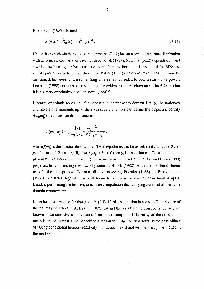
Brock et a1. (1987) defined

(3.12)

Under the hypothesis that {Yt} is an iid process, (3.12) has an asymptotic normal distribution

with zero mean and variance given in Brock et a1. (1987). Note that (3.12) depends on nand

E which the investigator has to choose. A much more thorough discussion of the BDS test

and its properties is found in Brock and Potter (1992) or Scheinkman (1990). It may be

mentioned, however, that a rather long time series is needed to obtain reasonable power.

Lee et a1. (1992) contains some small-sample evidence on the behaviour of the BOS test but

it is not very conclusive; see Terasvirta (1990b).

Linearity of a single series may also be tested in the frequency domain. Let {Yt} be stationary

and have finite moments up to the sixth order. Then we can define the bispectral density

f( Wj,Wj) of Yt based on third moments and

wherej{wD is the spectral density ofYt. Two hypotheses can be tested: (i) ifj{wj,wj) == 0 then

Yt is linear and Gaussian, (ii) if b( Wj,Wj) == bo > 0 then Yt is linear but not Gaussian, i.e., the

parameterized linear model for {Yt} has non-Gaussian errors. Subba Rao and Gabr (1980)

proposed tests for testing these two hypothesis. Hinich (1982) derived somewhat different

tests for the same purpose. For more discussion see e.g. Priestley (1988) and Brockett et a\.

(1988). A disadvantage of these tests seems to be relatively low power in small samples.

Besides, performing the tests requires more computation than carrying out most of their time

domain counterparts.

It has been assumed so far that g == 1 in (3.1). If this assumption is not satisfied, the size of

the test may be affected. At least the BOS test and the tests based on bispectral density are

known to be sensitive to departures from that assumption. If linearity of the conditional

mean is tested against a well-specified alternative using LM type tests, some possibilities

of taking conditional heteroskedasticity into account exist and will be briefly mentioned in

the next section.

18

3.3. Constancy of conditional variance

The assumption g == 1 is also a testable hypothesis. However, because conditional hetero­

skedasticity is discussed elsewhere in this volume, testing g == 1 against nonconstant

conditional variance is not considered here. This concerns not only testing linearity against

ARCH but also testing it against random coefficient linear regression; see e.g. Nicholls and

Pagan (1985) for further discussion on the latter situation.

Iff == 0 and g == 1 are tested jointly, a typical LM or LM type test is a sum of two separate

LM (type) tests for f == 0 and g == 1, respectively. This is the case because under this joint

null hypothesis the information matrix is block diagonal; see Granger and Terasvirta (1992,

chapter 6). Higgins and Bera (1989) derived a joint LM test against bilinearity and ARCH.

On the other hand, testing f == 0 when g =f. 1 is a more complicated affair than it is when g ==

1. If g is parameterized, the null model has to be estimated under conditional heteroskedas­

ticity. Besides, it may no longer be possible to carry out the test making use of a simple

auxiliary regression, see Granger and Terasvirta (1992). If g is not parameterized but g =f 1

is suspected then the tests described in section 3.1 as well as RESET and the Tsay test can

be made robust against g " 1. Davidson and MacKinnon (1985) and Wooldridge (1990)

described techniques for doing this. The present simulation evidence is not yet sufficient to

fully evaluate their performance in small samples.

4. SPECIFICATION OF NONLINEAR MODELS

If linearity tests indicate the need for a nonlinear model and economic theory does not

suggest a completely specificied model, then the structure of the model has to be specified

from the data. This problem also exists in nonparametric modelling as a variable selection

problem because the lags needed to describe the dynamics of the process are usually

unknown; see Auestad and Tj0stheim (1991) and Tj0stheim and Auestad (1991a,b). To

specify univariate time series models, Haggan et al. (1984) devised a specification technique

based on recursive estimation of parameters of a linear autoregressive model. The parame­

ters of the model were assumed to change over time in a certain fashion. Choosing a model

from a class of state-dependent models, see Priestley (1980, 1988), was carried out by

examining the graphs of recursive estimates. Perhaps because the family of state-dependent

models is large and the possibilities thus many, the technique is not easy to apply.

If the class of parametric models to choose from is more restricted, more concrete specifi-

19

cation methods may be developed. (For instance, Box and Jenkins (1970) restricted their

attention to linear ARMA models.) Tsay (1989) presented a technique making use of

linearity tests and visual inspection of some graphs to specify a model from the class of

threshold autoregressive models. It is easy to use and seems to work well. Chen and Tsay

(1990) considered the specification of functional-coefficient autoregressive models whereas

Chen and Tsay (1991) extended the discussion to additive functional coefficient regression

models. The key element in that procedure is the use of arranged local regressions in which

the observations are ordered according to a transition variable. Lewis and Stevens (1991a)

applied multivariate adaptive regression splines (MARS), see Friedman (1991), to specify

adaptive spline threshold autoregressive models. Terasvirta (1990a) discussed the specifi­

cation of smooth transition autoregressive models. This technique was generalized to

smooth transition regression models in Granger and Terasvirta (1992, chapter 7) and will

be considered next.

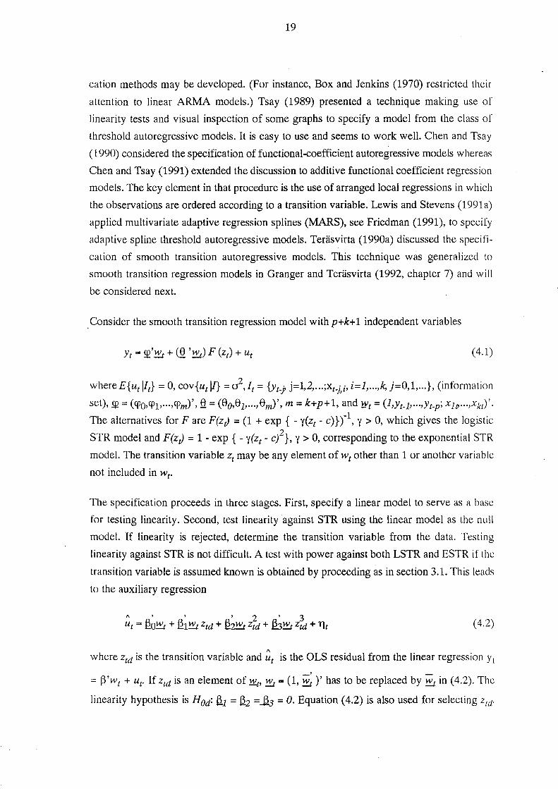
.Consider the smooth transition regression model withp+k+1 independent variables

(4.1 )

where E{ ut lIt} = 0, cov{ ut II} = a2,lt = {Yt-p j=1,2, . .. ;xt_j,i, i=l, ... ,k, j=O,l, ... }, (information

set), m = (CPO,CP1,···,CPm)', ft = (80,8 z, ... , 8m)', m = k+p+ 1, and tl't = (l,Yt-z,···,Yt-p; x 1p···,Xkt)'·

The alternatives for Fare F(zJ = (1 + exp { - Y(Zt - e)} rl, Y > 0, which gives the logistic

STR model and F(zJ = 1 - exp { - Y(Zt - e/}, Y > 0, corresponding to the exponential STR

model. The transition variable Zt may be any element of wt other than 1 or another variable

not included in w("

The specification proceeds in three stages. First, specify a linear model to serve as a hase

for testing linearity. Second, test linearity against STR using the linear model as the null

model. If linearity is rejected, determine the transition variable from the data. Testing

linearity against STR is not difficult. A test with power against both LSTR and ESTR if the

transition variable is assumed known is obtained by proceeding as in section 3.1. This leads

to the auxiliary regression

(4.2)

" where Ztd is the transition variable and ut is the OLS residual from the linear regression y l

= j3'wt + u{' If Ztd is an element of l:!4, ~ = (1, ~ )' has to be replaced by ~ in (4.2). The

linearity hypothesis is HOd: f21 = f22 =J13 = O. Equation (4.2) is also used for selecting Ztd'

20

The test is carried out for all candidates for Ztd, and the one yielding the smallest p-value is

selected if that value is sufficiently small. If it is not, the model is taken to be linear. This

procedure is motivated as follows. Suppose there is a true STR model with transition variable

Ztd that generated the data. Then the LM type test against that alternative has optimal power

properties. If an inppropriate transition variable is selected for the test, the resulting test may

still have power against the true alternative but the power is less than if the correct transition

variable is used. Thus the strongest rejection of the null hypothesis suggests that the

corresponding transition variable be selected. For more discussion of this procedure see

Terasvirta (1990a,c) and Granger and Terasvirta (1992, chapter 6 and 7). If linearity is

rejected and a transition variable selected, then the third step is to choose between LSTR

and ESTR models. This can be made by testing a set of nested null hypotheses within (4.2): * * * they are H 03: i23 = 0, H 02: i22 = 01i23 = 0 and H 01: i21 = 01i22 = i23 = O. The test results

contain information that is used in making the choice; see Granger and Terasvirta (1992,

chapter 7).

Specifying the lag structure of (4.1) could be done within (4.2) using an appropriate model

selection criterion but there is little experience about the success of such a procedure. In the

existing applications, a general-to-specific approach based on estimating nonlinear STR (or

STAR) models has mostly been used.

The model specification problem also arises in nonparametric time series modelling. Taking

model (2.5) as a starting-point, there lS the question of which lags

Xl-il , ... , Xt-ip ; Yt-h , ... , Yt-jq should be included in the model. Furthermore it should be

investigated whether the functions f and g are linear or nonlinear and whether they arc

additive or not. Moreover, if interaction terms are included, how should they be modelled

and, more generally, can the nonparametric analysis suggest functional forms such as the

smooth transition or threshold function or an ARCH type function for conditional variance?

These are problems of exploratory data analysis for nonlinear time series, and relatively

little nonparametric work has been done in the area. Various graphical model indicators

have been tried out in Tong (1990, chapter 7), Haggan et al. (1984) and Auestad and

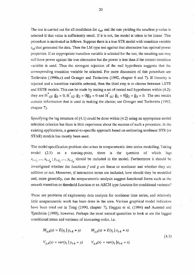
Tj0stheim (1990), however. Perhaps the most natural quantities to look at are the lagged

conditional mean and variance of increasing order, i.e.

My,iY) = E(Yt I Yt-k = y)

(4.3)

Vy key) = var(Yt I Yt-k = Y) . ,

21

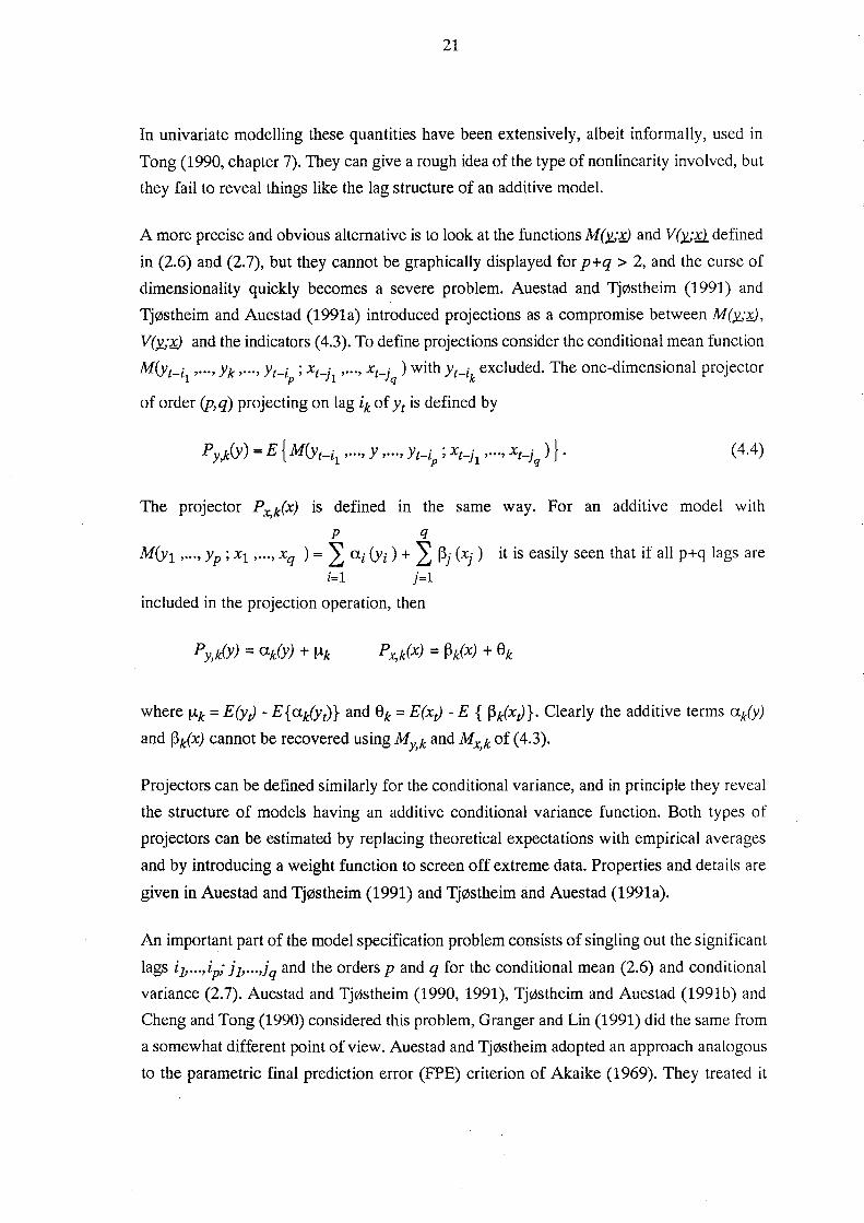
In univariate modelling these quantities have been extensively, albeit informally, used in

Tong (1990, chapter 7). They can give a rough idea of the type of nonlinearity involved, but

they fail to reveal things like the lag structure of an additive model.

A more precise and obvious alternative is to look at the functions M()!;~ and V(~J·±2. defined

in (2.6) and (2.7), but they cannot be graphically displayed for p+q > 2, and the curse of

dimensionality quickly becomes a severe problem. Auestad and Tj0stheim (1991) and

Tj0stheim and Auestad (1991a) introduced projections as a compromise between M()!.;~,

V()!...·~ and the indicators (4.3). To define projections consider the conditional mean function

M(Yt-il

, ••• , Yk , ... , Yt-ip

; xt-h , ... , xt-jq ) with Yt-ik

excluded. The one-dimensional projector

of order (p,q) projecting on lag ik of Yt is defined by

(4.4)

The projector Pxk(x) is defined in the same way. For an additive model with , p q

M(YI ,"', Yp ; xl,···, Xq ) = ~ ai (Yi ) + ~ Pj (Xj) it is easily seen that if all p+q lags are i=l j=l

included in the projection operation, then

where Ilk = E(yJ - E{aiYt)} and Ok = E(xJ - E { PixJ}. Clearly the additive terms aiY)

and Pk(x) cannot be recovered using My,k and Mx,k of (4.3).

Projectors can be defined similarly for the conditional variance, and in principle they reveal

the structure of models having an additive conditional variance function. Both types of

projectors can be estimated by replacing theoretical expectations with empirical averages

and by introducing a weight function to screen off extreme data. Properties and details are

given in Auestad and Tj¢stheim (1991) and Tj0stheim and Auestad (1991a).

An important part of the model specification problem consists of singling out the significant

lags i1, ... ,ip; h, ... ,jq and the orders p and q for the conditional mean (2.6) and conditional

variance (2.7). Auestad and Tj0stheim (1990, 1991), Tj0stheim and Auestad (1991b) and

Cheng and Tong (1990) considered this problem, Granger and Lin (1991) did the same from

a somewhat different point of view. Auestad and Tj0stheim adopted an approach analogous

to the parametric final prediction error (FPE) criterion of Akaike (1969). They treated it

22

only in the univariate case, but it is easily extended to the multivariate situation.

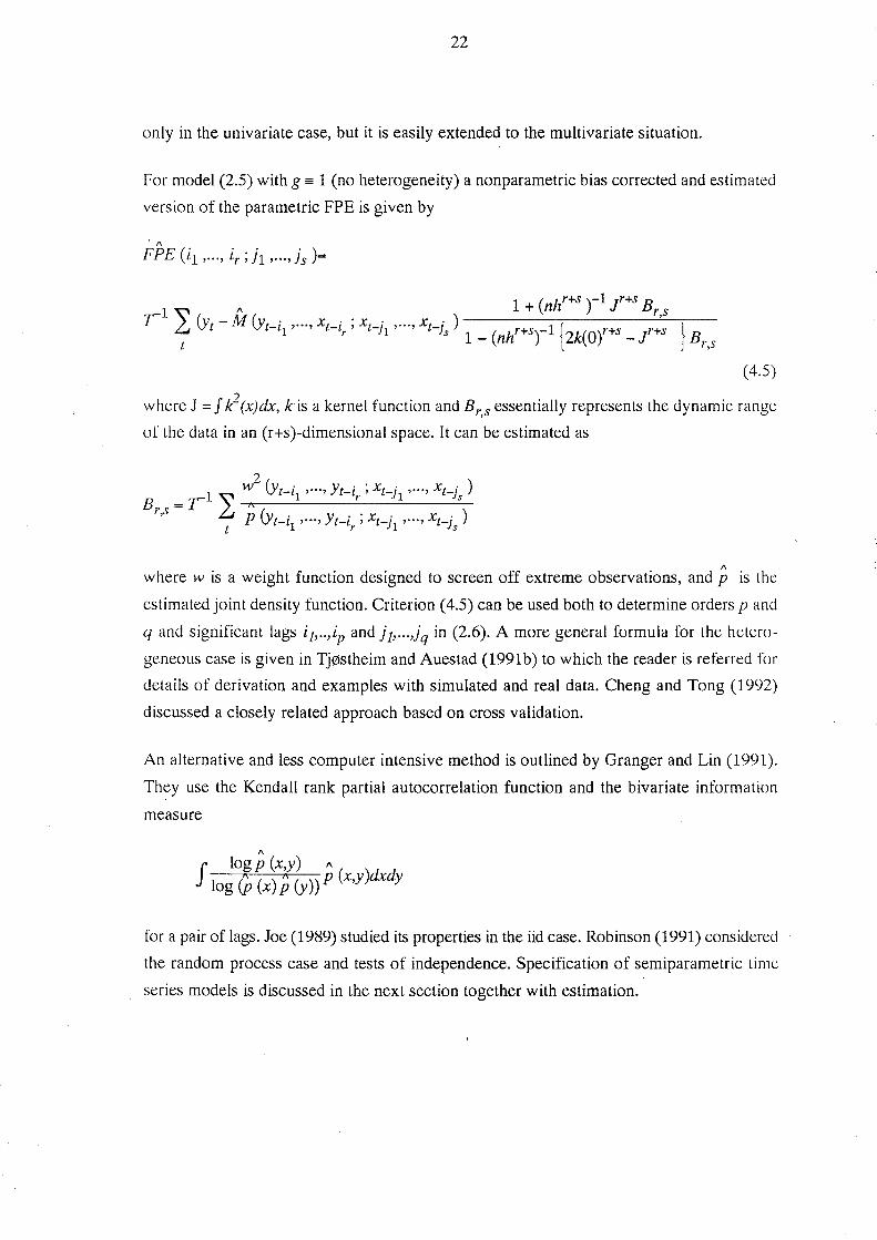
For model (2.5) with g == 1 (no heterogeneity) a nonparametric bias corrected and estimated

version of the parametric FPE is given by

1\

FPE (i1 , ... , ir;h ,···,js)=

1 ( I r+s )-1 Jr+s B 1 ~ 1\ + n 7, r,s

r L,; (Yt - M (Yt-i1 , ••• , xt-i ; Xt-jl , ... , Xt_j ) r+s 1 { r+s r+s t r s 1-(nh r 2k(O) -J

( 4.5)

where J = J k2 (x)dx, k is a kernel function and Br s essentially represents the dynamic range , of the data in an (r+s)-dimensional space. It can be estimated as

2 w (Yt-i , ... , Yt-i ; Xt_j , ... , Xt_j )

Br s = r 1 2:" 1 r 1 s , t P (Yt-i

1 , ••• , Yt-i

r ; Xt-h , ... , Xt-js )

1\

where w is a weight function designed to screen off extreme observations, and p is the

estimated joint density function. Criterion (4.5) can be used both to determine orders p and

q and significant lags i1, .. ,ip and h, ... ,jq in (2.6). A more general formula for the hetero­

geneous case is given in Tj0stheim and Auestad (1991b) to which the reader is referred for

details of derivation and examples with simulated and real data. Cheng and Tong (1992)

discussed a closely related approach based on cross validation.

An alternative and less computer intensive method is outlined by Granger and Lin (1991).

They use the Kendall rank partial autocorrelation function and the bivariate information

measure

1\

f logp (x,y) 1\

log (p (x) p (y)) p (x,y)dxdy

[or a pair of lags. Joe (1989) studied its properties in the iid case. Robinson (1991) considered

the random process case and tests of independence. Specification of semiparametric time

series models is discussed in the next section together with estimation.

23

5. ESTIMATION IN NONLINEAR TIME SERIES

5.1. Estimation of parameters in parametric models

For parametric nonlinear models, conditional nonlinear least squares is the most common

estimation technique. If the errors are normal and independent, this is equivalent to

conditional maximum likelihood. The theory derived for dynamic nonlinear models (3.1)

with g == 1 gives the conditions for consistency and asymptotic normality of the estimators.

For an account, see e.g. Gallant (1987, chapter 7). Even more general conditions were

recently laid out in Potscher and Prucha (1990, 1991). These conditions may be difficult to

verify in practice, so that the asymptotic standard deviation estimates, confidence intervals

and the like have to be interpreted with care. For discussions of estimation algorithms see

e.g. Quandt (1983), Judge et al. (1985, appendix B) and Bates and Watts (1988). The

estimation of parameters in (2.2) may not always be straightforward. Local minima may

occur, so that estimation with different starting-values is recommended. Estimation of y in

transition function (2.3) may create problems if the transition is rapid because there may not

be sufficiently many observations in the neighbourhood of the point about which the

transition takes place. The convergence of the estimate sequence may therefore be slow, see

Bates and Watts (1988, p. 87) and Granger and Tedisvirta (1992, chapter 7). For simulation

evidence and estimation using real economic data sets see also Granger et al. (1992),

Luukkonen (1990), Tedisvirta (1990a) and Terasvirta and Anderson (1991). Model (2.2)

may even be a switching regression model in which case y is not finite and cannot be

estimated. In that case its estimated value will grow until the iterative estimation algorithm

breaks down. An available alternative is then to fix y at some sufficiently large value and

estimate the remaining parameters conditionally on that value.

The estimation of parameters becomes more complicated if the model contains lagged errors

as the bilinear model does. Subba Rao and Gabr (1984) outlined a procedure for the

estimation of a bilinear model based on maximizing the conditional likelihood. Quick

preliminary estimates may be obtained using a long autoregression to estimate the residuals

and OLS for estimating the parameters keeping the residuals fixed. This is possible because

the bilinear model has a simple structure in the sense that it is linear in the parameters if we

regard the lagged residuals as observed. Granger and Terasvirta (1992, chapter 7) suggested

this alternative.

If the model is a switching regression or threshold autoregressive model, nonlinear least

squares is an inapplicable technique because of the irregularity of the sum of squares or

likelihood function. The problem consists of the unknown switch-points or thresholds for

24

which unique point estimates are not available as long as the number of observations is

finite. Tsay (1989) suggested specifying (approximate) switch-points from "scatterplots of

t-values" in ordered (according to the switching variable) recursive regressions. As long as

the recursion stays in the same regime, the t-value of a coefficient estimate converges to a

fixed value. When observations from another regime are added into the regression, the

coefficient estimates start changing and the t-values deviating. Tsay (1989) contains

examples. The estimation of parameters in regimes is carried out by ordinary least squares.

Chan (1988) showed (in the univariate case) that if the model is stationary and ergodic, the

parameter estimates, including those of the thresholds, are strongly consistent.

5.2. Estimation of nonparametric functions

In nonparametric estimation the most common way of estimating the conditional mean (2.6)

and variance (2.7) is to apply the so-called kernel method. It is based on a kernel function

. k(x) which typically is a real continuous, bounded, symmetric function integrating to one.

Usually it is required that k(x) ~ 0 for all X, but sometimes it is advantageous to allow k(x)

to take negative values, so that we may have f x2 k(x)dx = O. The kernel method is explained

in much greater detail in the chapter by HardIe on nonparametric estimation.

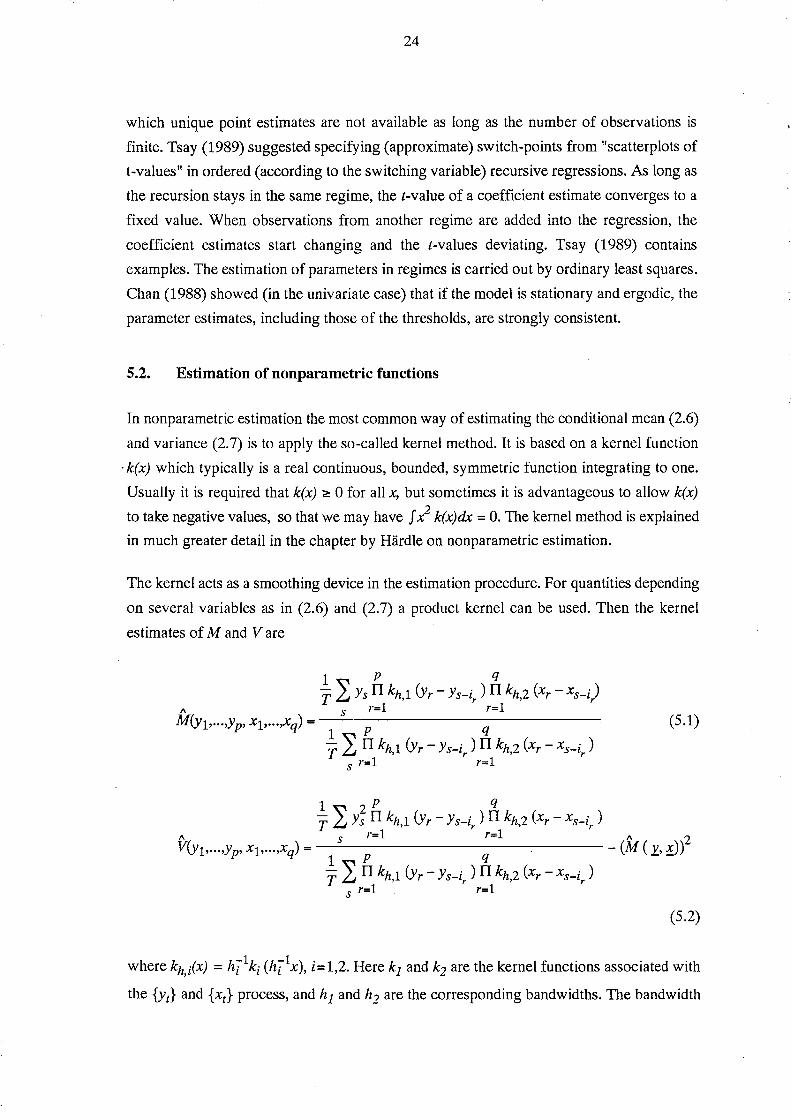
The kernel acts as a smoothing device in the estimation procedure. For quantities depending

on several variables as in (2.6) and (2.7) a product kernel can be used. Then the kernel

estimates of M and Vare

12: p q

T Ys n kh 1 (yr - Ys-i ) n kh 2 (xr - xs-i ) , r' r

" s r=1 r=1 M(Y1,oo"Yp, Xl>oo"xq) = ----------------

1 p q

T ~ n kh 1 (yr - Ys-i ) n kh 2 (xr - xs-i ) L.J, r' r

S r=1 r=1

(5.1)

1 2: ? P q , r' r T Y; n kh 1 (yr - Ys-i ) n kh 2 (xr - xs-i )

" s r=1 r=1 "2 V(Y1,oo"Yp' Xl>oo"xq) = - (M ( 1:, ~»

1 p q

T ~ n kh 1 (yr - Ys-i ) n kh 2 (xr - xs-i ) L.J, r' r S r=1 r=1

(5.2)

where kh,lx) = hj1ki (hj1x), i=1,2. Here k1 and k2 are the kernel functions associated with

the {Yt} and {Xt} process, and h1 and h2 are the corresponding bandwidths. The bandwidth

25

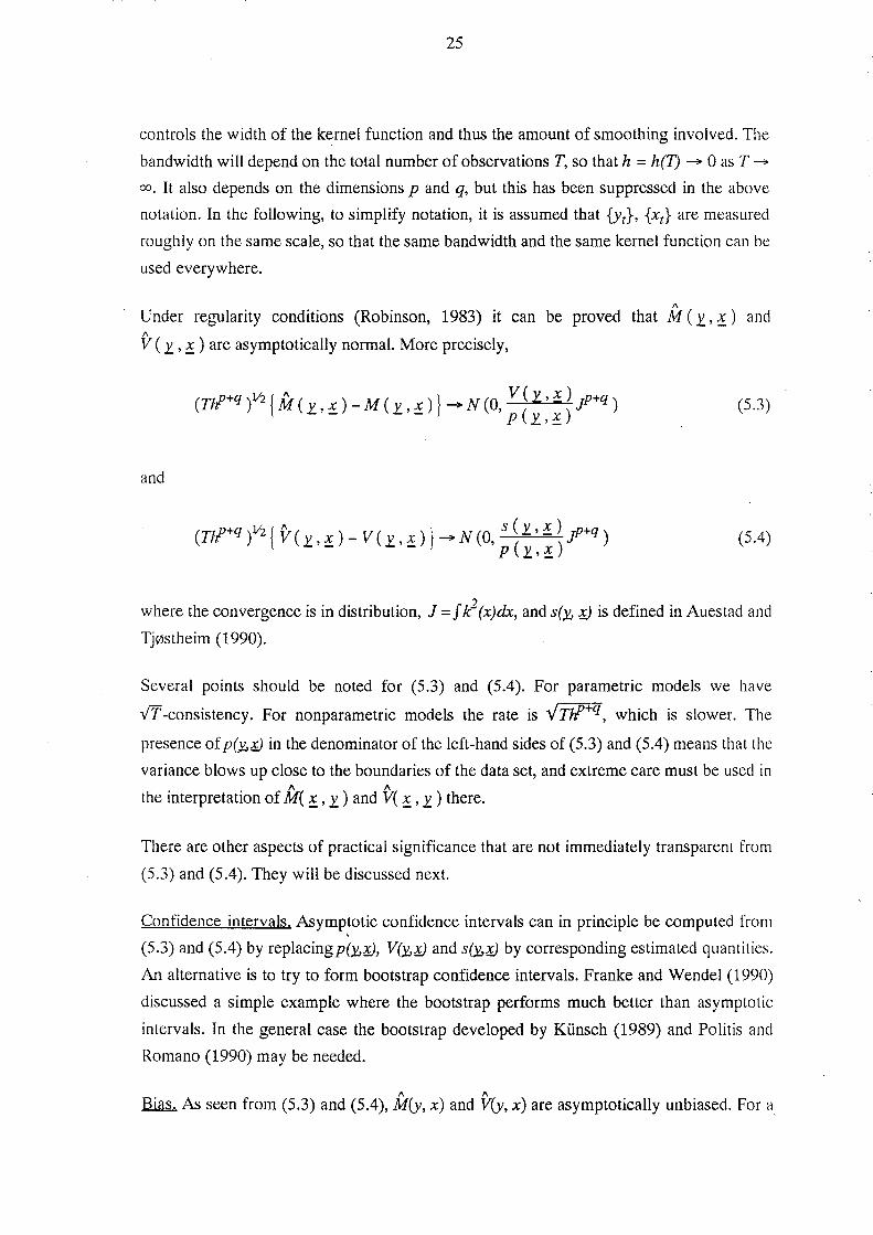
controls the width of the kernel function and thus the amount of smoothing involved. The

bandwidth will depend on the total number of observations T, so that h = h(T) - ° as T --;.

00. It also depends on the dimensions p and q, but this has been suppressed in the above

notation. In the following, to simplify notation, it is assumed that {Yt}, {Xt} are measured

roughly on the same scale, so that the same bandwidth and the same kernel function can be

used everywhere.

1\

Under regularity conditions (Robinson, 1983) it can be proved that M (J:, ~) and 1\

V (1:., ~) are asymptotically normal. More precisely,

(Tlf+q

)V2 { if (J:, ~ ) - M ( J: , ~ ) } - N (0, ; ~ ~: ~ ~ jp+q ) (5.3)

and

(Tlf+q t2 { V (J:, ~) - V (J:, ~) } - N (0, ; ~ ~::~ jp+q) (5.4)

where the convergence is in distribution, j = f k2 (x)dx, and s()!., ~ is defined in Auestad and

Tj0stheim (1990).

Several points should be noted for (5.3) and (5.4). For parametric models we have

fl-consistency. For nonparametric models the rate is V TJl+7J, which is slower. The

presence ofp(~;y in the denominator of the left-hand sides of (5.3) and (5.4) means that the

variance blows up close to the boundaries of the data set, and extreme care must be used in 1\ 1\

the interpretation of M( ~ , J: ) and V( ~ , J: ) there.

There are other aspects of practical significance that are not immediately transparent from

(5.3) and (5.4). They will be discussed next.

Confidence intervals. Asymptotic confidence intervals can in principle be computed from , (5.3) and (5.4) by replacingp()!.,;Y, V()!.,;Y and s()!.,;Y by corresponding estimated quantities.

An alternative is to try to form bootstrap confidence intervals. Franke and Wendel (1990)

discussed a simple example where the bootstrap performs much better than asymptotic

intervals. In the general case the bootstrap developed by Kiinsch (1989) and Politis and

Romano (1990) may be needed.

1\ 1\

Bias. As seen from (5.3) and (5.4), M(y, x) and V(y, x) are asymptotically unbiased. For a

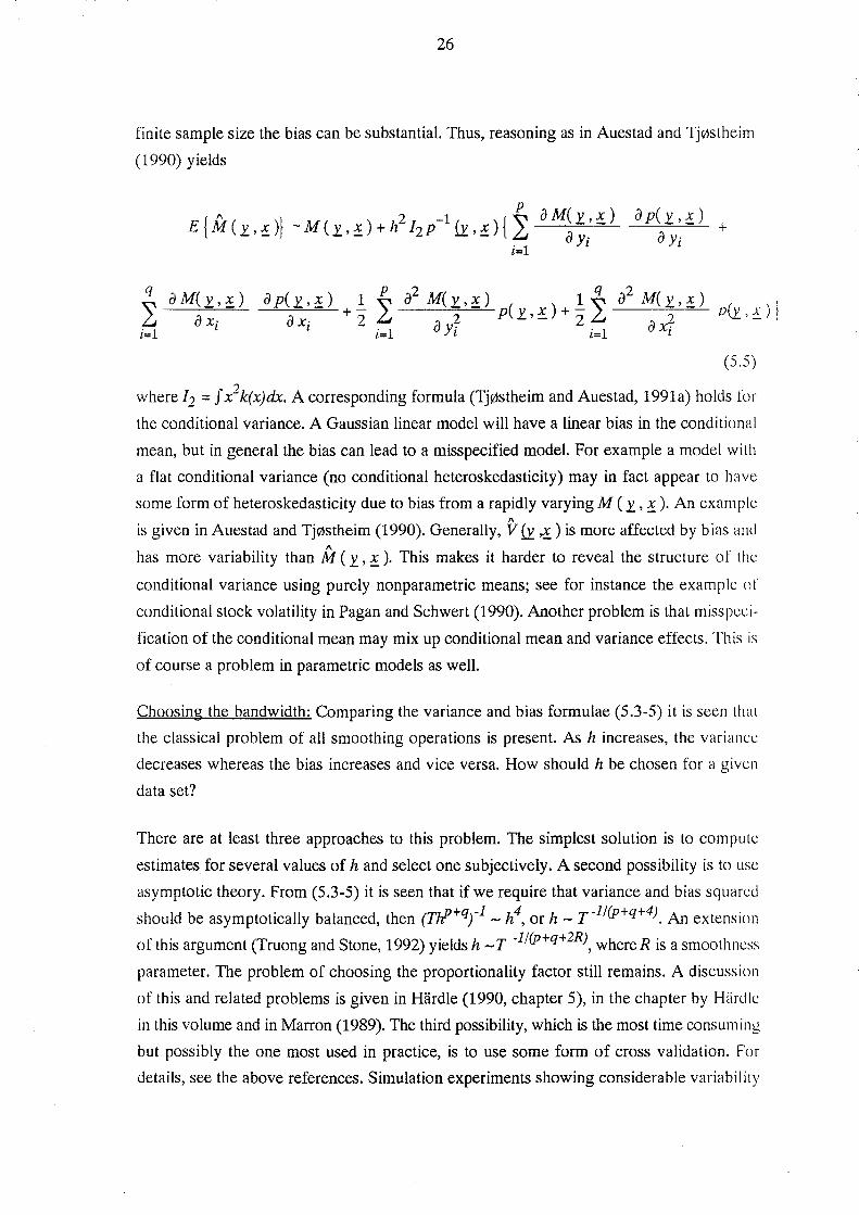
26

finite sample size the bias can be substantial. Thus, reasoning as in Auestad and Tj0stheim

(1990) yields

a pC Y.., x ) +

~ a M(y", x) L.J a xi

P 2 q 2 a p( Y.. , x) +! " a M( Y.. , x ) ( ) 1" a M( Y.. , x) Of "Y , A_" ) I

ax. 2 L.J 2 P Y..,! +"2 L.J 2 \.L r L i=l aYi i=l aXi i=l

(5.5)

where 12 = f x2k(x)dx. A corresponding formula (Tj0stheim and Auestad, 1991a) holds for

the conditional variance. A Gaussian linear model will have a linear bias in the conditional

mean, but in general the bias can lead to a misspecified model. For example a model with

a flat conditional variance (no conditional heteroskedasticity) may in fact appear to have

some form of heteroskedasticity due to bias from a rapidly varying M (Y.. , ! ). An exampk 1\

is given in Auestad and Tj0stheim (1990). Generally, V IT .!) is more affected by bias and 1\

has more variability than M (y",!). This makes it harder to reveal the structure of the

conditional variance using purely nonparametric means; see for instance the example or conditional stock volatility in Pagan and Schwert (1990). Another problem is that misspeei­

fication of the conditional mean may mix up conditional mean and variance effects. This is

of course a problem in parametric models as well.

Choosing the bandwidth: Comparing the variance and bias formulae (5.3-5) it is seen that

the classical problem of all smoothing operations is present. As h increases, the variance

decreases whereas the bias increases and vice versa. How should h be chosen for a given

data set?

There are at least three approaches to this problem. The simplest solution is to compute

estimates for several values of h and select one subjectively. A second possibility is to use

asymptotic theory. From (5.3-5) it is seen that if we require that variance and bias squared

should be asymptotically balanced, then (Tlf+qr1 - ",,4, or h - T -l/(p+q+4). An extension

of this argument (Truong and Stone, 1992) yields h - T -l/(p+q+2R), whereR is a smoothness

parameter. The problem of choosing the proportionality factor still remains. A discussioll

of this and related problems is given in HardIe (1990, chapter 5), in the chapter by H~irdle

in this volume and in Marron (1989). The third possibility, which is the most time consuming

but possibly the one most used in practice, is to use some form of cross validation. For

details, see the above references. Simulation experiments showing considerable variahility

27

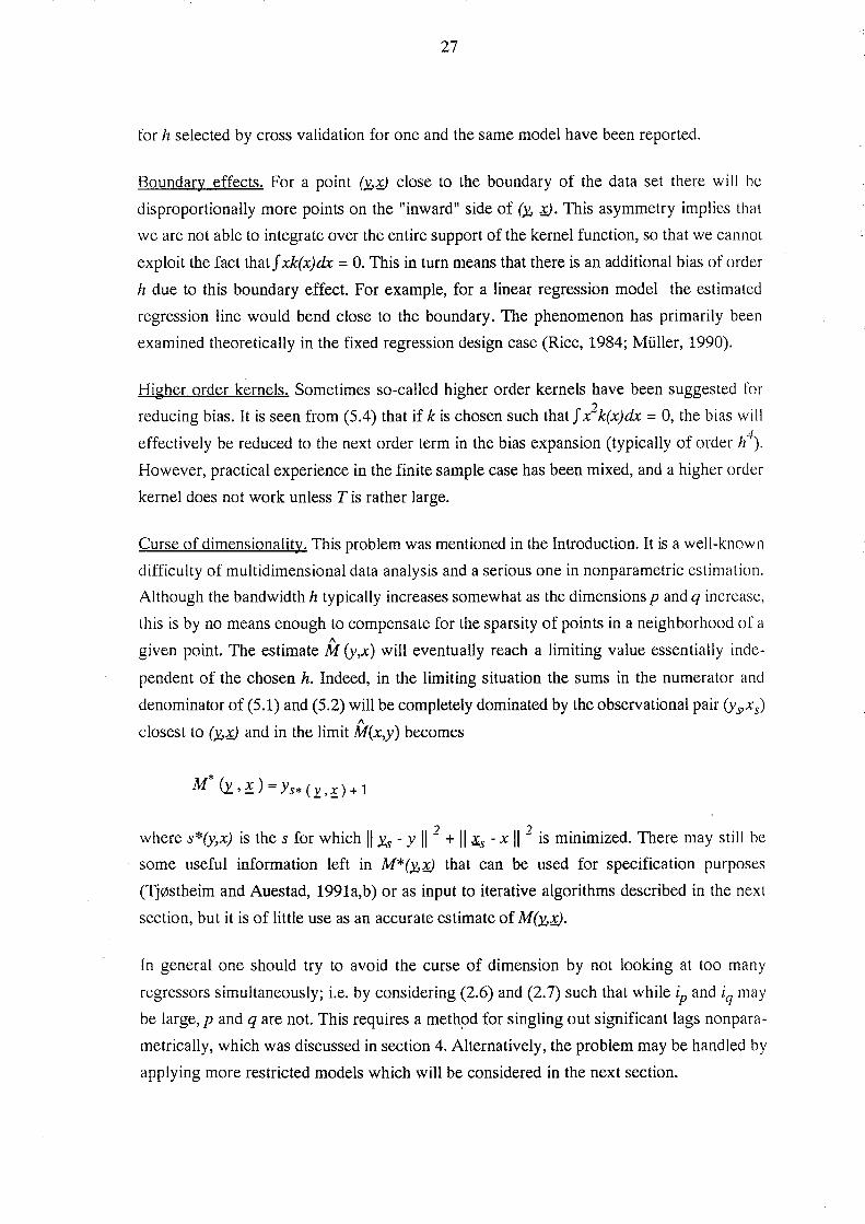
for h selected by cross validation for one and the same model have been reported.

Boundary effects. For a point (x,.r) close to the boundary of the data set there will he

disproportionally more points on the "inward" side of (x, .r). This asymmetry implies that

we are not able to integrate over the entire support of the kernel function, so that we cannot

exploit the fact thatf xk(x)dx = o. This in turn means that there is an additional bias of order

h due to this boundary effect. For example, for a linear regression model the estimated

regression line would bend close to the boundary. The phenomenon has primarily been

examined theoretically in the fixed regression design case (Rice, 1984; Milller, 1990).

Higher order kernels. Sometimes so-called higher order kernels have been suggested for

reducing bias. It is seen from (5.4) that if k is chosen such thatfik(x)dx = 0, the bias will

effectively be reduced to the next order term in the bias expansion (typically of order h\ However, practical experience in the finite sample case has been mixed, and a higher order

kernel does not work unless T is rather large.

Curse of dimensionality. This problem was mentioned in the Introduction. It is a well-known

difficulty of multidimensional data analysis and a serious one in nonparametric estimation.

Although the bandwidth h typically increases somewhat as the dimensions p and q increase,

this is by no means enough to compensate for the sparsity of points in a neighborhood of a 1\

given point. The estimate M (y,x) will eventually reach a limiting value essentially inde-

pendent of the chosen h. Indeed, in the limiting situation the sums in the numerator and

denominator of (5.1) and (5.2) will be completely dominated by the observational pair (ysxs) 1\

closest to (x,..r) and in the limit M(x,y) becomes

M* (y , :! ) = y s* ( 1:: , ! ) + 1

where s*(y,x) is the s for which II Xs - Y 112 + 11.!s -x 112 is minimized. There may still he

some useful information left in M*(x,..r} that can be used for specification purposes

(Tj0stheim and Auestad, 1991a,b) or as input to iterative algorithms described in the next

section, but it is of little use as an accurate estimate of M(x,.r).

In general one should try to avoid the curse of dimension by not looking at too many

regressors simultaneously; i.e. by considering (2.6) and (2.7) such that while ip and iq may

be large, p and q are not. This requires a meth!Jd for singling out significant lags nonpara­

metrically, which was discussed in section 4. Alternatively, the problem may be handled by

applying more restricted models which will be considered in the next section.

28

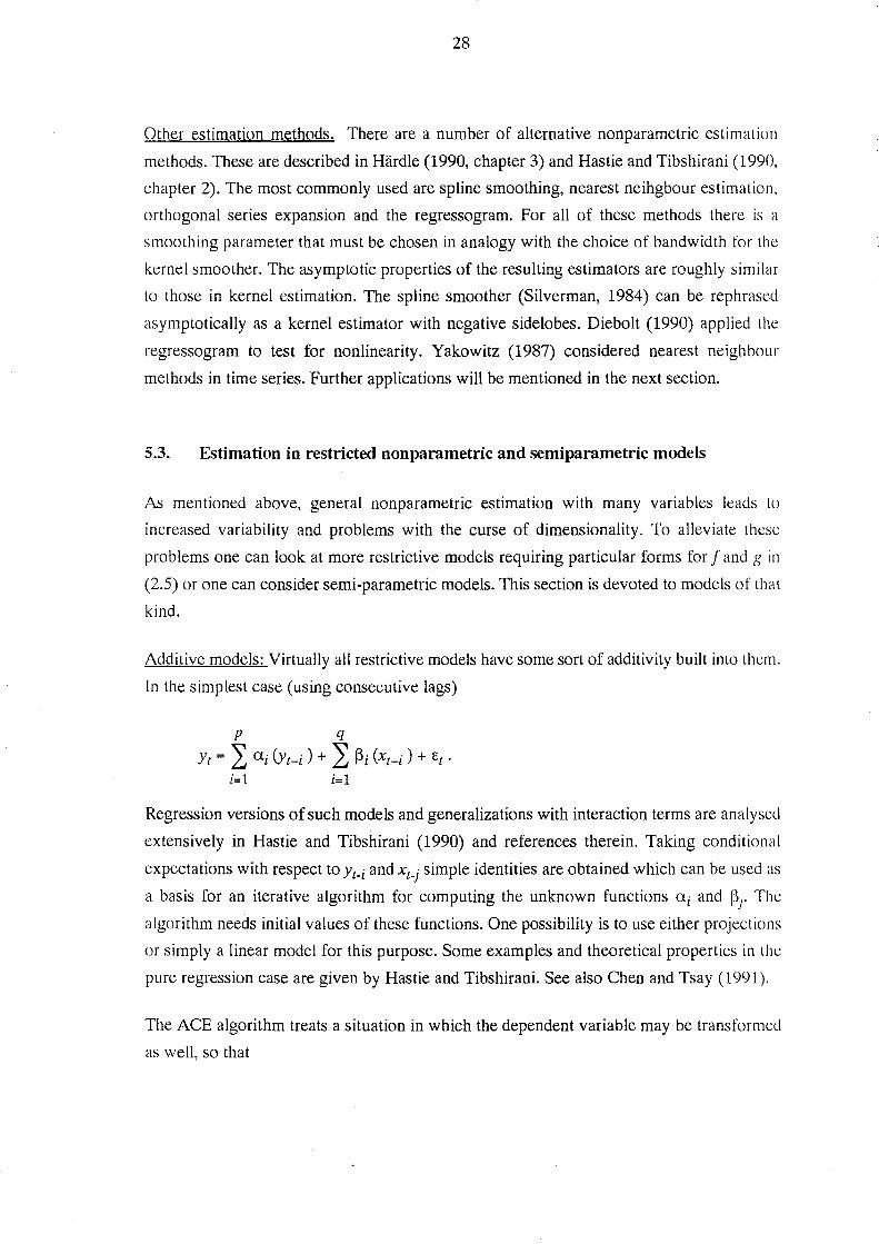
Other estimation methods. There are a number of alternative nonparametric estimation

methods. These are described in Hardie (1990, chapter 3) and Hastie and Tibshirani (1990,

chapter 2). The most commonly used are spline smoothing, nearest neihgbour estimation,

orthogonal series expansion and the regressogram. For all of these methods there is a

smoothing parameter that must be chosen in analogy with the choice of bandwidth for the

kernel smoother. The asymptotic properties of the resulting estimators are roughly similar

to those in kernel estimation. The spline smoother (Silverman, 1984) can be rephrased

asymptotically as a kernel estimator with negative sidelobes. Diebolt (1990) applied the

regressogram to test for nonlinearity. Yakowitz (1987) considered nearest neighbour

methods in time series. Further applications will be mentioned in the next section.

5.3. Estimation in restricted nonparametric and semi parametric models

As mentioned above, general nonparametric estimation with many variables leads to

increased variability and problems with the curse of dimensionality. To alleviate these

problems one can look at more restrictive models requiring particular forms for f and g in

(2.5) or one can consider semi-parametric models. This section is devoted to models of that

kind.

Additive models: Virtually all restrictive models have some sort of additivity built into them.

In the simplest case (using consecutive lags)

p q

Yt = 2: ai (Yt-i ) + 2: ~i (xt-i ) + Ct •

i=l i=l

Regression versions of such models and generalizations with interaction terms are analysed

extensively in Hastie and Tibshirani (1990) and references therein. Taking conditional

expectations with respect to Yt-i and Xt_j simple identities are obtained which can be used as

a basis for an iterative algorithm for computing the unknown functions ai and f)j" The

algorithm needs initial values of these functions. One possibility is to use either projections

or simply a linear model for this purpose. Some examples and theoretical properties in the

pure regression case are given by Hastie and Tibshirani. See also Chen and Tsay (1991).

The ACE algorithm treats a situation in which the dependent variable may be transformed

as well, so that

29

The algorithm is perhaps test suited for a situation where Uj = 0 for all i, so that there is a

clear distinction between the input and output variables. The method was developed in

Breiman and Friedman (1985). Some curious aspects of the ACE algorithm are highlighted

in Hastie and Tibshirani (1990, p. 184-186). In view of the above comments it is perhaps

not surprising that in a time series example Hallman (1990) obtained better results by using

a version of backfitting (Tibshirani, 1988) than with the ACE algorithm.

Chen and Tsay (1990) considered a univariate model allowing certain interactions. Their

functional coefficient autoregressive (FCAR) model is given as

Yt = II (Yt-i1

, ... , Yt-ik ) Yt-1 + ... + Jp (Yt-i1 ,"', Yt-ik ) Yt-p + Et

with ik:s p. By ordering the observations according to some variable or a known combination

bf them to an "ordered" local regression the authors proposed an iterative procedure for

evaluatingh, ... ,jp and gave some theoretical properties. The procedure simplifies dramati­

cally if all the fj are one-dimensional. The authors fitted an FCAR model of this type to the

chicken pox data of Sughihara et al. (1990). The fitted model seemed to point at a threshold

autoregressive model. The forecasts from such a model subsequently fitted to the data had

a MSE at least 30 % smaller than a seasonal ARMA model used as a comparison for

forecasting 4-11 months ahead.

Projection pursuit type models. In our notation these models can be written as

r

Yt = ~ ~j (I} Y t-1 + se}:! t-1 ) + et j=1

where ~j' j=i, ... ,r, are unknown functions, Yj and mj are unknown vectors determining the

direction of the j-th projector, and .lLt-l' -It-l are as in (2.5). An iterative procedure (Friedman

and Stuetzle, 1981) exists for deriving optimal projectors (projection pursuit step) and

functions ~j' The curse of dimensionality is avoided since in the smoothing part of the

algorithm it is exploited that ~j is a function of one scalar variable. For time series data,

experience with this method is limited. A small simulation study Granger and Teriisvirta

(1991) conducted gave marginal improvements compared to linear model fitting for the

particular nonlinear models they considered. Projection pursuit models are related to neural

network models, but for the latter the functions ~j are assumed known and often ~j = ~,j =

i, ... ,r, thus giving a parametric model class. The fitting of neural network models is

30

discussed in White (1989).

Regression trees. splines and MARS. Assume a model of form

and approximate I(~~ in terms of simple basis functions B/~~ so that lappr (~,rJ =

L Cj Bj (1:.,!). In the regression tree approach (Breiman et aI., 1984) lappr is built up

j

recursively from indicator functions Bj (~,rJ = I {.6:,,rJ E Rj } and the regions Rj are

partitioned in the next step of the algorithm according to a certain pattern. As can be expected

there are problems in fitting simple smooth functions like the linear model.

Friedman (1991) in his MARS (Multivariate Adaptive Regression Splines) methodology

has made at least two important new contributions. First, to overcome the difficulty in fitting

simple smooth functions Friedman proposed not to automatically eliminate the parent region

Rj in the above recursive scheme for creating subregions. In subsequent iteration both the

parent region and its corresponding subregions are eligible for further partitioning. This

allows for much greater flexibility. The second contribution is to replace step functions by

products of linear left and right truncated regression splines. The products make it possible

to include interaction terms. For a detailed discussion the reader is referred to Friedman

(1991).

Lewis and Stevens (1991a) applied MARS to time series, both simulated and real data. As

for most of the techniques discussed in this section a number of input parameters are needed.

Lewis and Stevens recommended running the model for several sets of parameters and then

selecting a final model based on various specification/fitting tests. They fitted a model to

the sunspot data which has 3 one-way, 3 two-way and 7 three way interaction terms. The

MARS model produced better overall forecasts of the sunspot activity than the models

applied before. In Lewis and Stevens (1991b) riverflow is fitted against temperature and

precipitation and good results obtained. There are as yet no applications to economic data.

The MARS technology appears very promising but must of course be tested more exten­

sively on real and simulated data sets. No asymptotic theory with confidence intervals is

available yet.

Stepwise series expansion of conditional densities. In a sense the conditional density p(Yt I J!.t-z, ~-1) is the most natural quantity to look at in a joint modelling of {yv Xt} since predictive

distributions as well as the conditional mean and variance can all be derived from this

31

quantity. Gallant and Tauchen (1990) used this fact as their starting point.

The conditional density is estimated, to avoid the curse of dimensionality, by expanding it

in Hermite polynomials. These are centred and scaled so that the conditional mean M()!..,~

and variance V()!..,.g playa prominent role. As a first approximation they are supposed to be

linear Gaussian and of ARCH type, respectively.

Gallant et a1. (1990) looked at econometric applications, notably to stock market data. In

particular, they investigated the relationship between volatility of stock prices and volume.

A main finding was that an asymmetry in the volatility of prices when studied by itself mon.:

or less disappears when volume is included as an additional conditional variable. Possible

asymmetry in the conditional variance function (univariate case) has recently been studied

by a number of investigators using both parametric and nonparametric methods; see Engle

and Ng (1991) and references therein.

Semiparametric models. Another way of trying to eliminate the difficulties in evaluating

high-dimensional conditional quantities is to assume nonlinear and nonparametric depend­

ence in some of the predictors and parametric and usually linear dependence in others. An

illustrative example is given by Engle et a1. (1986) who modelled electricity sales using a

number of predictor variables. It is natural to assume the impact of temperature on electrici t y

consumption to be nonJinear, as both high and low temperatures lead to increased consump­

tion, whereas a linear relationship may be assumed for the other regressors. A similar

situation arose in Shumway et a1. (1988) which is a study of mortality as a function of weather

and pollution variables in the Los Angeles region.

In the context of model (2.5) with a linear dependence on lags of Yt and nonlinearity with

respect to the exogenous variable {Xt}, we have

Yt = £'y t-1 + f(! t-1 ) + c("

The modelling technique would depend somewhat on the dimension of Kt-l' In the case

where the argument of f is scalar, it can be incorporated in the backfitting algorithm of Hastie

and Tibshirani (1990, p. 118). Under quite general assumptions it is possible to obtain

v'T-consistency for the parametric part as demonstrated by Heckman (1986) and Robinson

(1988). Powell et a1. (1989) developed the theory further and gave econometric applications.

32

6. EVALUATION OF ESTIMATED MODELS

After estimating a nonlinear time series model it is necessary to evaluate its properties to

see if the specified and estimated model may be regarded as an adequate description of the

relationship it was constructed to characterize. The residuals of the model can be subjected

to various tests such as those against ARCH and normality. At least in the parametric case

linearity of the time series was tested, and the same tests may now be performed on the

residuals to see if the model adequately characterizes the nonlinearity the tests previously

suggested. Note, however, that the asymptotic distribution of the Ljung-Box test statistic of

no autocorrelation based on estimated residuals is not available, as the correct number of

degrees of freedom is known only for the linear ARMA case. However, considering residual

autocorrelations as such is informative. One should also study the stability of the model,

which generally can only be done numerically by simulating the model without noise. The

exogenous variables should be set on a constant level, for instance to equal their sample

means. If the solution path diverges, the model should be rejected and respecification

attempted. Other examples of a solution are a limit cycle or a stable singular point. See e.g.

Ozaki (1985) for further discussion.

The out-of-sample prediction of the model is an important part of the evaluation process.

The precision of the forecasts should be compared to those from the corresponding linear

model. However, as mentioned in the Introduction, the results also depend on the data during

the forecasting period. If there are no observations in the range in which nonlinearity of the

model makes an impact, then the forecasts cannot be expected to be more accurate than

those from a linear model. The check is thus negative: if the forecasts from the nonlinear

model are significantly less accurate than those from the corresponding linear one, then the

nonlinear specification should be reconsidered.

7. EXAMPLE

As a parametric example of the specification, estimation and evaluation cycle we shall

consider the seasonally unadjusted logarithmic U.S. industrial output 1960(1) to 1986(4).

This is one of the series analyzed in Terasvirta and Anderson (1991). The four quarter

differences (growth rate) contain strong fluctuations, and the problem is to find an adequate

description of the series. Selecting the linear. autoregressive model using AIC yields an

AR(6) model. Results of the linearity tests against STAR when the delay, d, is varied from

1 to 9 are given in Table 1. The test is based on an auxiliary regression like (4.2) which is

33

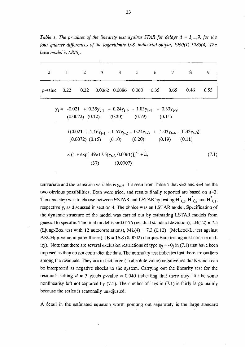
Table 1. The p-values of the linearity test against STAR for delays d = 1, ... ,9, for the

four-quarter differences of the logarithmic U.S. industrial output, 1960(1)-1986(4). The

base model is AR(6).

d 1 2 3 4 5 6 7 8

p-value 0.22 0.22 0.0062 0.0086 0.060 0.35 0.65 0.46

Yt = -0.021 + 0.35Yt_l + 0.24Yt_3 - 1.03Yt_4 + 0.33Yt_9

(0.0072) (0.12) (0.20) (0.19) (0.11)

+(0.021 + 1.16Yt_l - 0.57Yt_2 - 0.24Yt_3 + 1.03Yt_4 - 0.33Yt_9)

(0.0072) (0.15) (0.10) (0.20) (0.19) (0.11)

1 1\

x (1 + exp[-49x17.5(Yt_3-0.0061)]Y + ut

(37) (0.0007)

9

0.55

(7.1)

univariate and the transition variable is Yt-d. It is seen from Table 1 that d=3 and d=4 are the

two obvious possibilities. Both were tried, and results finally reported are based on d=3. * * * The next step was to choose between ESTAR and LSTAR by testing H 03, H 02 and H 01>

respectively, as discussed in section 4. The choice was an LSTAR model. Specification of

the dynamic structure of the model was carried out by estimating LSTAR models from

general to specific. The final model is s=0.0176 (residual standard deviation), LB(12) = 7.5

(Ljung-Box test with 12 autocorrelations), ML( 4) = 7.3 (0.12) (McLeod-Li test against

ARCH; p-value in parentheses), JB = 16.8 (0.0002) (Jarque-Bera test against non-normal­

ity). Note that there are several exclusion restrictions of type Cf>j = -8j in (7.1) that have been

imposed as they do not contradict the data. The normality test indicates that there are outliers

among the residuals. They are in fact large (in absolute value) negative residuals which can

be interpreted as negative shocks to the system. Carrying out the linearity test for the

residuals setting d = 3 yields p-value = 0.040 indicating that there may still be some

nonlinearity left not captured by (7.1). The number of lags in (7.1) is fairly large mainly

because the series is seasonally unadjusted.

A detail in the estimated equation worth pointing out separately is the large standard

34

deviation of y. In order to obtain an idea of the size of y the exponent of the transition function

is standardized by multiplying it by the inverse of the estimated standard deviation of Yt

which equals 17.5. Seen against that background y = 49 is a large number indicating that

the transition function changes from zero to unity or vice versa very rapidly whenYt_3 crosses

0.0061. However, the uncertainty of y seems large. This is the situation described in Bates

and Watts (1988, p. 87). The large standard deviation reflects the fact that a wide range of

values of y around 49 would give a very similar transition function. It is not due to linearity

of the series. Many more observations in the neighbourhood of c would be needed to estimate

y accurately. As a matter of fact, the residual variance of (7.1) is less than two-thirds of that

of the AR(6) model, which is a large reduction.

The long-term solution of (7.1) is interesting. The realizations starting from a given set of

starting values display cycles of varying length but no regular limit cycle seems to appear.

If the starting-values are changed slightly, another cyclical realization emerges which

gradually drifts apart from the previous one. Thus any change in the starting-values affects

the long-run solution. It is also instructive to study the characteristic polynomials of (7.1)

at different values of the logistic transition function F (see (4.1», zero and unity being most

interesting as the extreme values. When F = 0, which corresponds to the recession, the

equation has two pairs of complex roots with moduli 1.11 and 1.01, respectively. The roots

of the expansion regime (F = 1) are a stationary complex pair with modulus 0.75. Thus the

output recovers from a recession swiftly as explosive roots are needed to characterize that.

On the other hand, there is little else in this characterization than large negative shocks

pushing the industry from an expansion into a recession.

One-quarter-ahead forecasts for 1987-1988 not shown here contribute little to the analysis

because the output growth fluctuates little during that period. Both linear and nonlinear

models have the root mean square prediction error way below the residual standard deviation

of the nonlinear model.

The general conclusion is that there is no inherent nonlinearity in the series. For instance, it

cannot be argued that the series is asymmetric, which has been a recent topic of nonlinear

time series analysis. Nonlinear structure is needed mainly to describe the recovery of

industrial production from a large negative shock. This is also seen by comparing the

residuals of (7.1) and the AR(6) model, which also is a useful way of evaluating the nonlinear

model. For more discussion of this and similar models for a few other OEeD countries the

reader is referred to Tedisvirta and Anderson (1991). Applications of bivariate STR models

can be found in Granger et aI. (1992); see also Granger and Terasvirta (1992, chapter 10).

35

8. CONCLUSIONS

This chapter is an attempt at an overview of various ways of modelling nonlinear economic

relationships. Since nonlinear time series models and methods are a very large field, not all

important developments have been covered. The emphasis has been on model building, and

the modelling cycle of linearity testing, model specification, parameter or nonparametric

function estimation and model evaluation has been highlighted. The estimation of fully

specified nonlinear theory models like disequilibrium models has not been the topic here.

A majority of results concern the estimation of the conditional mean of a process whereas

the conditional variance has received less attention. This is in part because conditional

heteroskedasticity is discussed in a separate chapter. Random coefficient models also belong

under that heading and have not been considered here. Furthermore, this presentation retlecL~

the belief that economic phenomena are more naturally characterized by stochastic than

deterministic models, so that deterministic chaos and its applications to economics have

only been briefly mentioned in the discussion.

At present the number of applications of nonlinear time series models in economics is still

fairly limited. Many techniques discussed here are as yet relatively untested. However, the

situation may change rather rapidly, so that in a few years the possibilities of evaluating the

empirical success of the present and new techniques will be essentially better than now.

36

REFERENCES

Akaike, H. (1969). Fitting autoregressions for predictions. Annals of the Institute of Statistical Mathematics 21, 243-247.

Anderson, B.D.O. and J.B. Moore (1979). Optimal filtering. Englewood Cliffs, NJ: Prentice-Hall.

Andrews, D.W.K. (1990). Tests for parameter instability and structural change with un­known change point. Cowles Foundation for Research in Economics, unpublished manuscript.

Auestad, B. and D. Tj0stheim (1990). Identification of nonlinear time series: First order characterization and order determination. Biometrika 77, 669-687.

Auestad, B. and D. Tj0stheim (1991). Functional identification in nonlinear time series. In: G. Roussas, ed. Nonparametric functional estimation and related topics. Amsterdam: Kluwer Academic Publishers, 493-507.

Barnett, W.A., J. Powell and G.E. Tauchen, eds. (1991). Nonparametric and semi­parametric methods in econometrics and statistics. Proceedings of the 5th. International Symposium in Economic Theory and Econometrics. Cambridge: Cambridge University Press.

Bates, D.M. and D.G. Watts (1988). Nonlinear regression analysis & its applications. New York: Wiley.

Box, G.E.P. and·G.M. Jenkins (1970). Time series analysis. forecasting and control. San Francisco: Holden-Day.

Breiman, L. and J.H. Friedman (1985). Estimating optimal transformations for multiple regression and correlation (with discussion). Journal of the American Statistical Association 80, 580-619.

Breiman, L., J.H. Friedman, R. Olshen and CJ. Stone (1984). Classification and regres­sion trees. Belmont, CA: Wadsworth.

Brock, W.A., Dechert, W.D. and AJ. Scheinkman (1987). A test for independence based on the correlation dimension. Working paper, University of Wisconsin-Madison, Social Systems Research Institute.

Brock, W.A. and S.M. Potter (1992). Nonlinear time series and macroeconometrics. Unpublished manuscript.

Brockett, P.L., MJ. Hinich and D. Patterson (1988). Bispectral-based tests for the detec­tion of Gaussianity and linearity in time series. Journal of the American Statistical Association 83, 657-664.

37

Brown, R.L., J. Durbin and J.M. Evans (1975). Techniques for testing the constancy of regression coefficients over time. Journal of the Royal Statistical Society B, 37, 149-192 (with Discussion).

Chan, K.S. (1990). Testing for threshold autoregression. Annals of Statistics 18, 1886-1894.

Chan, K.S. (1991). Percentage points of likelihood ratio tests for threshold autoregres­sion. Journal of the Royal Statistical Society B, ~, 691-696.

Chan, K.S. and H. Tong (1986). On estimating thresholds in autoregressive models. , Journal of Time Series Analysis 1, 179-190.

Chan, K.S. and H. Tong (1990). On likelihood ratio tests for threshold autoregression. Journal of the Royal Statistical Society B, .5,2,469-476.

Chen, P. and R.H. Day, eds. (1992). Non-linear dynamics and evolutionary economics. Cambridge, MA: MIT Press (forthcoming).

Chen, R. and R. Tsay (1990). Nonlinear time series analysis: A functional coefficient autoregressive model approach. Preprint. Department of Statistics, Texas A & M

University.

Chen, R. and R. Tsay (1991). Nonlinear additive ARX models. Preprint. Graduate School of Business, University of Chicago.

Cheng, B. and H. Tong (1992). On consistent nonparametric order determination and chaos. Journal of the Royal Statistical Society, B (forthcoming).

Chow, G.c. (1960). Testing for equality between sets of coefficients in two linear regres­sions. EconOmetrica 28, 591-605.

Davidson, R. and J.G. MacKinnon (1985). Heteroskedasticity-robust tests in regressions directions. Annales de l'INSEE 59/60, 183-218.

Davies, R.B. (1977). Hypothesis testing when a nuisance parameter is present only under the alternative. Biometrika 74, 247-254.

De Gooijer, J.G. and K. Kumar (1991). Some recent developments in non-linear time series modelling, testing and forecasting. Unpublished paper.

Desai, M. (1984). Econometric models of the share of wages in national income, U.K., 1855-1965. In: R.M. Goodwin, M. Kruger and A. Vercelli, eds. Nonlinear models of fluctuating growth. Lecture Notes in Economics and Mathematical Systems No. 228. New York: Springer Verlag. .

Diebolt, J. (1990). Testing the functions defining a nonlinear autoregressive time series. Stochastic Processes and their Applications.3.Q., 85-106.

38

Engle, R.F., C.W.J. Granger, J. Rice and A. Weiss (1986). Semiparametric estimates of the Relation between weather and electricity sales. Journal of the American Statistical Association 8l, 310-320.

Engle, R.F. and V. Ng (1991). Measuring and testing the impact of news on volatility. University of California, San Diego, Department of Economics, Discussion Paper No. 91-15.

Ertel, J.E. and E.B. Fowlkes (1976). Some algorithms for linear spline and piecewise multiple linear regression. Journal of the American Statistical Association 71,

640-648.

Franke, J. and M. Wendel (1990). A bootstrap approach for nonlinear autoregressions. Some preliminary results. Preprint, to appear in Proceedings of the International Conference on Bootstrapping and Related Techniques, Trier, June 1990.

Friedman, J.H. (1991). Multivariate adaptive regression splines (with discussion). Annals of Statistics 12.. 1-141.

Friedman, J.H. and W. Stuetzle (1981). Projection pursuit regression. Journal of the American Statistical Association 7.§., 817-823.

Gallant, A.R. (1981). On the bias in flexible functional forms and an essentially unbiased form: The Fourier Flexible Form. Journal of Econometrics ll, 211-245.

Gallant, A.R. (1987). Nonlinear statistical models. New York: Wiley.

Gallant, A.R. and G. Tauchen (1990). A nonparametric approach to nonlinear time series analysis: Estimation and simulation. Preprint, to appear in IMA volumes on Mathematics and its Applications, Springer Verlag.

Gallant, A.R., P.E. Rossi and G. Tauchen (1990). Stock prices and volume. Graduate School of Business, University of Chicago, working paper.

Granger, C.W.J. and J.J. Hallman (1991a). Nonliner transformations of integrated time series. Journal of Time Series Analysis.12.. 207-224.

Granger, C.W.J. and J.J. Hallman (1991b). Long-memory processes with attractors. Oxford Bulletin of Economics and Statistics 111l-26.

Granger, C.W.J. and J.L. Lin (1991). Nonlinear correlation coefficients and identifica­tion of nonlinear time series models. University of California, San Diego, Department of Economics, Discussion Paper.

Granger, C.W.J. and P. Newbold (1986). Forecasting economic time series, 2nd edition. Orlando, FL: Academic Press.

Granger, C.W.J. and T. Tedisvirta (1991). Experiments in modeling nonlinear relation­ships between time series. Proceedings of the NATO/Santa Fe Conference on Non-

39

linear Modelin~ and Forecasting (forthcoming).

Granger, C.W.J. and T. Terasvirta (1992). Modelling nonlinear dynamic relationships. Oxford: Oxford University Press (forthcoming).

Granger, C.WJ., T. Terasvirta and H.M. Anderson (1992). Modelling non-linearity over the business cycle. In: J.H. Stock and M.W. Watson, eds. New research on business

cycles. indicators and forecasting. Chicago: Chicago University Press (forthcoming).

Haggan, V., S.M. Heravi and M.B. Priestley (1984). A study of the application of state­dependent models in nonlinear time series analysis. Time Series Analysis ~, 69-102.

Haggan, V. and T. Ozaki (1981). Modelling non-linear random vibrations using an ampli­tude-dependent autoregressive time series model. Biometrika Q8., 189-196.

Hallman, J.J. (1990). Nonlinear integrated series, co integration and application. PhD Thesis. University of California, San Diego, Department of Economics.

Hansen, B.E. (1990). Lagrange multiplier tests for parameter instability in non-linear models. Paper presented at the Sixth World Congress of the Econometric Society, Barcelona.

HardIe, W. (1990). Applied nonparametric regression. Oxford: Oxford University Press.

Harvey, A.c. (1990). Econometric analysis of time series. 2nd edition. Cambridge, MA: MIT Press.

Hastie, TJ. and R.J. Tibshirani (1990). Generalized additive models. London: Chapman and Hall.

Heckman, N. (1986). Spline smoothing in a partly linear model. Journal of the Statistical Society, 11 ~ 244-248.

Higgins, M. and A.K. Bera (1989). A joint test for ARCH and bilinearity in the regression model. Econometric Reviews L 171-181.

Hinich, M.J. (1982). Testing for gaussianity and linearity of a stationary time series. Journal of Time Series Analysis .1169-176.

Joe, H. (1989). Estimation of entropy and other functionals of a multivariate density. Annals of the Institute of Statistical Mathematics 11. 683-697.

Judge, G.G., W.E. Griffiths, R.C. Hill, H. Liitkepohl and T.-C. Lee (1985). The theory and practice of econometrics, 2nd edition. New York: Wiley.

Keenan, D.M. (1985). A Tukey non-additivity type test for time series nonlinearity. Biometrika 7.l. 39-44.

Kramer, W., W. Ploberger and R. Alt (1988). Testing for structural change in dynamic

40

models. Econometrica ~ 1335-1370.

Kiinsch, H. (1989). The jackknife and the bootstrap for general stationary observations. Annals of Statistics.l1, 1217-1241.

Lasota, A. and M.C. Mackey (1987). Stochastic perturbation of dynamical systems: The weak convergence of measures. Journal of Mathematical Analysis and Applications.ua, 232-248.

Lee, T.-H., White, H. and C.W.J. Granger (1992). Testing for neglected nonlinearity in time series models. A comparison of neural network methods and alternative tests.

Journal of Econometrics (forthcoming).

Lewis, P.A.W. and J.G. Stevens (1991a). Nonlinear modeling of time series using multi­variate adaptive regression splines (MARS). Journal of the American Statistical Association 8Q.. 864-877.

Lewis, P.A.W. and J.G. Stevens (1991b). Semi-multivariate nonlinear modeling of time series using multivariate adaptive regression splines (MARS). Preprint, Naval Post­

graduate School.

Liu, T., C.WJ. Granger and W. Heller (1991). Using the correlation exponent to decide if an economic series is chaotic. University of California, San Diego, Department of Economics, Discussion Paper No. 91-21.

Luukkonen, R. (1990). On linearity testing and model estimation in non-linear time series analysis. Helsinki: Finnish Statistical Society.

Luukkonen, R., P. Saikkonen and T. Terasvirta (1988a). Testing linearity in univariate time series. Scandinavian Journal of Statistics .ll, 161-175.

Luukkonen, R., P. Saikkonen and T. Terasvirta (1988b). Testing linearity against smooth transition autoregression. Biometrika 72, 491-499.

Maddala, G.S. (1977). Econometrics. New York: McGraw-Hill.

Maddala, G.S. (1986). Disequilibrium, self-selection and switching models. In: Z. Griliches and M.D. Intriligator, eds. Handbook of econometrics. Vol. 3. Amsterdam: North-Holland, 1634-1688.

Marron, S. (1989). Automatic smoothing parameter selection: A survey. In: A. Ullah, ed. Semiparametric and nonparametric econometrics. Heidelberg: Physica-Verlag, 65-86.

Miiller, H.G. (1990). Smooth optimum kernel estimators near endpoints. Preprint, University of California, Davis.

Nicholls, D.F. and A.R. Pagan (1985). Varying coefficient regression. In: EJ. Hannan, P.R. Krishnaiah and M.M. Rao, eds. Handbook of statistics, Vol. 5. Amsterdam:

Elsevier, 413-449.

42

Time Series Analysis 1, 185-208.

Robinson, P.M. (1988). Root-N-consistent semiparametric regression. Econometrica ~ 931-954.

Robinson, P.M. (1991). Consistent nonparametric entropy-based testing. Review of Economic Studies (forthcoming).

Saikkonen, P. and R Luukkonen (1988). Lagrange multiplier tests for testing non­linearities in time series models. Scandinavian Journal of Statistics 15, 55-68.

Scheinkman, J.A. (1990). Nonlinearities in economic dynamics. Economic Journal 100, Supplement, 33-48.

Shumway, RH., A.S. Azari and Y. Pawitan (1988). Modeling mortality fluctuations in Los Angeles as functions of pollution and weather effects. Environmental Research ~ 224-241.

Silverman, B.W. (1984). Spline smoothing: the equivalent variable kernel method. Annals of Statistics .l2, 898-916.

Stensholt, B.K. and D. Tj(3stheim (1987). Multiple bilinear time series models. Journal of Time Series Analysis .8., 221-233.

Stinchcombe, M. and H. White (1989). Universal approximations using feedforward net­works with hon-sigmoid hidden layer activation functions. Proceedings of the International Joint Conference on Neural Networks. Washington. D.C. San Diego: SOS Printing, I: 613-618.

Subba Rao, T. and M.M. Gabr (1980). A test for linearity of stationary time series. Journal of Time Series Analysis 1,145-158.

Subba Rao, T. and M.M. Gabr (1984). An introduction to bispectral analysis and bilinear time series models. Lecture Notes in Statistics 24, New York: Springer.

Sughihara, G. and R.M. May (1990). Nonlinear forecasting as a way of distinguishing chaos from measurement error in time series. Nature~, 734-741.

Terasvirta, T. (1990a). Specification, estimation, and evaluation of smooth transition autoregressive models. University of California, San Diego, Department of Economics, Discussion Paper No. 90-39.

Tedisvirta, T. (1990b). Power properties of linearity tests for time series. University of California, San Diego, Department of Economics, Discussion Paper No. 90-15.

Tedisvirta, T. (199Oc). Generalizing threshold autoregressive models. University of California, San Diego, Department of Economics, Discussion Paper No. 90-44.

Terasvirta, T. and H.M. Anderson (1991). Modelling nonlinearities in business cycles

44

Yakowitz, S. (1987). Nearest-neighbour methods for time series analysis. Journal of Time Series Analysis 8, 235-247.

1990:1 Holm, S.

1990:2 Holm, S. & Dahlbom, U

1991:1 Olofsson, Jonny

1991:2 Jonsson, Robert

1991:3 Holm, s. & Svensson, E.

1992:1 Terasvirta, T Tj¢stheim, D Granger, C W J

Abstract bootstrap confidence intervals in linear models.

On tests of equivalence

On some prediction meth6ds for categorical data

On the problem of optimal inference in the simple error component model for panel data

Statistical rank methods for ordinal categoricai data

Aspects of Modelling Nonlinear Time Series