unitte mc1 - nordtank measurement campaign (turbine and

UniTTe

DTU

Win

d E

ne

rgy

UniTTe – MC1 - Nordtank Measurement

Campaign (Turbine and Met Masts)

Andrea Vignaroli

DTU Wind Energy Report-I-0363

May 2016

Author: Andrea Vignaroli

Title: UniTTe – MC1 - Nordtank Measurement Campaign (Turbine and Met Masts)

Institute: Wind Energy

May 2016

Resume (mask. 2000 char.):

This report describes the instrumentation of the turbine and met masts used in the

first measurement campaign of the UniTTe project.

Contract no.: Innovationsfondens

1305-00024B

Project: UniTTe

http://www.unitte.dk/

Funding:

Innovation Fund Denmark

Pages:

Tables:

Figures:

References:

Technical University of Denmark

DTU Wind Energy Risø Campus Frederiksborgvej 399

DK-4000 Roskilde Denmark

www.vindenergi.dtu.dk

http://www.unitte.dk/

http://www.vindenergi.dtu.dk/

UniTTe – MC1 - Nordtank Measurement Campaign (Turbine and Met Masts)

Preface

This report is a deliverable (D3.11) of the UniTTe project. It describes the setup of the first

measurement campaign (MC1) regarding the met masts and wind turbine measurements

during the period where measurements were taken with the short range WindScanner and the

SpinnerLidar. Set up and measurements with the remote sensing instruments are described in

another report (D3.12). Analysis of the data is the focus of several other publications within

the project. The purpose of these two reports is to provide the necessary information about

the measurements for the data analysis.

UniTTe – MC1 - Nordtank Measurement Campaign (Turbine and Met Masts)

Content

1. Introduction 7

2. Experiment setup 7

3. Data inspection and quality check 17

4. Strain Gauges Calibrations 20

4.1 Line calibration ....................................................................................................................................... 20

4.2 Strain Gauge Calibration procedure ....................................................................................................... 21

4.3 Regression analysis ................................................................................................................................. 23

4.4 Zero determination ................................................................................................................................ 24

4.5 Results .................................................................................................................................................... 25

5. Database 27

6. Channel List in MySQL database 29

7. Accuracy on turbine yawing 32

8. Synchronization 35

9. Wind conditions during MC1 36

10. Thrust curve analysis 41

References 44

Thanks to 45

Error! Use the Home tab to apply Normal - Forside Overskrift 1 to the text that you want to appear here.

1. Introduction

The UniTTe project addresses the question of how best to characterize the wind when measuring the power

and loads on modern wind turbines through several measurements campaigns [www.UniTTe.dk]. The first

experiment took place on the Nordtank NTK 500/41 wind turbine situated at DTU Risø Campus. The primary

purpose of this measurement campaign was to measure the inflow to the Nordtank wind turbine with the

short range WindScanner and the SpinnerLidar. The set up and configuration of those instruments are

described in [1]. The second purpose was to assess the value of the spinner lidar measurements for the

turbine loads assessment.

The turbine is equipped with an extensive number of sensors monitoring and recording the mechanical loads

and acceleration on structure and components which have been recorded almost continuously during the

years. A detailed description of the sensors, acquisition system and history of the turbine is given in [2].

2. Experiment setup

The wind turbine is geographically located at the Risø Campus, about 6 km North of Roskilde as shown on

Figure 1Error! Reference source not found.. The wind turbine is placed on the foundation no 4, in a rather

gentle sloping terrain towards the area ‘Bløden’ on the west side of the Roskilde firth. The free undisturbed

inflow is from the dominant westerly wind direction.

The test wind turbine is a traditional Danish three-bladed stall regulated Nordtank, NTK 500/41 wind turbine

– see specifications in Table 1. Figures in brackets reflect results from post survey on turbine specs.

Figure 1 Aerial view of experiment setup

Table 1 Tubine specifications

Rotor Diameter 41.1m

Swept area 1320 m²

Rotational Speed 27.1 rpm

Measured tip angle -0.2º±0.2º

Tilt 2º

Coning 0º

Blade type LM 19.1

Blade profile[s] NACA 63-4xx & NACA FF-W3, equipped with vortex generators

Blade length 19.04 m

Blade chord 0.265 – 1.630 m

Blade twist 0.02 – 20.00 degrees

Air brakes Pivotal blade tips, operated in FS-mode

Mechanical brake High speed shaft, operated in FS-mode

Power regulation Passive aerodynamic stall

Gearbox Flender; ratio 1

Generator Siemens 500 kW, 4 poles, 690 V

Tower Type Conical steel tube, h=33.8 m

Hub height 36.0 m

Blade weight 1960 kg (2249 kg incl. Extender and bolts)

Rotor incl. Hub 9030 kg (9846 kg)

Tower head mass 24430 kg (25246kg)

Tower mass 22500 kg

The turbine is primarily used for energy production and tests and it is serviced on commercial conditions.

The turbine was installed in 1992 with a 37 m diameter rotor, which in 1994 was substituted with a 41 m

diameter rotor in combination with a rotor speed reduction to limit the power output.

Some relevant geometrical properties of the turbine were derived by measuring the position in space of

certain points. Such measurements was performed using a theodolite, which is

a surveying instrument with a rotating telescope for measuring horizontal and vertical angles capable to

measure distances with an accuracy of in the range of 1 mm. A graphical representation of such

measurements can be seen in Figure 2 below followed by the numerical values in Table 2

Figure 2 XY Measurements point taken with a theodolite of the Nordtank turbine.

N E Z

Reference_(stairs) 0.000 0.000 0.000

Tower1 -1.514 -0.952 1.754

Tower2 -1.852 -3.264 1.740

tower center -1.683 -2.108 1.747

Bladetip1 -18.159 -8.266 46.025

Bladetip2 13.033 8.805 43.939

Bladetip3 -4.621 0.283 14.089

Rotor center -3.249 0.274 34.684

NacLidarLowerleftleftside -2.250 -0.545 36.062

NacLidarUpperleftleftside -2.246 -0.566 36.803

alfa (deg) 33.322

horizontal distance lidar-rotorcenter 0.980

vertical distance lidar-rotorcenter 1.748

-20.000

-15.000

-10.000

-5.000

0.000

5.000

10.000

15.000

-10.000 -5.000 0.000 5.000 10.000

Stairs

Blade tip1

Blade tip2

Blade tip3

RotorCenter

lidar

TowerCent

alfa

rotor tilt 0.754 2.1

horizontal distance reference-towercenter 2.697

horizontal distance rotorcenter-towercenter

2.851

Horizontal distance reference-rotorcenter 0.153 Table 2 Geometrical measurements of the Nordtank Turbine relevant for the project. if not specified, all units in meters

Presently the experimental facility is instrumented as described in the following.

A meteorological mast is placed 2.5 (92.4m) rotor diameters in westerly direction (283°) from the wind

turbine. The mast is equipped for measurement of wind speed over the turbine rotor, wind direction, air

temperature, air barometric pressure and air humidity (Figure 3) Wind speed is measured by cup

anemometers and sonic anemometers that are able to measure the 3D wind vector allowing measuring also

wind direction. No wind vanes are present.

Figure 3 Tall mast

All cup anemometers are WindSensor P2546A type and recently calibrated from Deutsche WindGuard. The

information regarding the calibrations for the cup anemometers are reported in the table below (Table 3):

Table 3 Calibration information

Height (m) Mounting Serial Number Calibration date

18 North 2756 DTU-Vea 2076 15.07.2013 18 South 10103 - 2513 17.02.2014 27 South 10095 - 2527 18.06.2014 36 North 13861 - 2759 17.02.2014 36 South 13862 - 2760 17.02.2014 45 South 13863 - 2761 06.11.2013 54 North 14104 DTU-Vea 2790 16.07.2013 54 South 14107 DTU-Vea 2793 16.07.2013 57 Top mounted 14108 DTU-Vea 2794 15.07.2013

The installation is made in accordance with the recent IEC recommendations for both power performance

[4] and structural load measurements [5].

There is also another shorter met mast between turbine and the taller mast (at 48.7m from the turbine).

This is an older mast that was installed for turbine testing on smaller turbine not existing anymore. The short

met mast has been equipped for this experiment with a METEK 3D ultra sonic anemometer (model:

scientific/ former USA-1) on the top.

Figure 4 Setup for meteorological measurements

The structural loads on the turbine are monitored by strain gauges mounted at the blade root, on the main

shaft, at the tower top and at the tower bottom (Error! Reference source not found.) since 2010. The load

ignals from the blades include flapwise and edgewise bending moments at the blade root, measured by

strain gauges mounted on the blade root steel extenders. The gauge installation at 2.1m from rotor axis

enables measurements of both flap-wise and edge-wise bending moments in the rotating right handed

reference system of the rotor where the center of the rotor plane is the origin, the x-axis is the rotor axis of

rotation and z-axis is aligned with blade n.1. flapwise moment is therefore referred as My and edgewise

moment as Mx. The rotor is in 0-position when blade 1 is pointing vertically upwards. A sketch of one of the

three blades with the position of the strain gauges I shown in Figure 5.

Figure 5Structural load measurements in the blade root

The load measurement on the main shaft includes a torque sensor in front and right after the main bearings,

and two bending moments at a position behind the hub/main shaft flange – in a rotating reference system

(Figure 7). The gauge location enables measurements of bending moments in two directions, perpendicular

to each other in a rotating reference system. The two bending moments combined with the rotor position

are used to determine the rotor bending moments in yaw and tilt direction - in a nacelle reference system.

Additionally accelerometers are positioned on the gearbox and on the rear of the nacelle frame.

The tower loads includes torque at the tower top and bending moments in two directions at the tower

bottom at 3.5 m from the ground, as shown on in a (fixed) tower reference system (East West refers to the

turbine-mast direction and North-South to the direction oriented 90 degrees to the previously defined E-W).

The angle between N-S direction and the geographical North is 15.37 Degrees.

Figure 6 Structural load measurements on the main shaft including distances from the rotor plane.

Figure 7 Rotating reference system for load measurements on the shaft.

Figure 8 Power and structural load measurements on the welded tubular steel tower

A PC-based data acquisition system has been designed to monitor and collect data from the wind turbine

sensors.

The output signals from all sensors are conditioned to the +/- 5 V range. Analogue signals are either

continuously varying (strain gauges, temperature…), digital types such as train of pulses (rotational speed,

anemometer…) or on/off levels (status signals for brake, blade tips and generator modes). All signals - except

outputs from voltage and current transformers - are connected to one of three RISØ P2558A data acquisition

units (DAU), each of which provides 16 analogue input channels and 6 general-purpose digital input

channels. The analogue inputs are converted into 16-bit quantities. Data from all channels are assembled in

a binary telegram, each data occupying 16 bits. The telegram is preceded by two synchronization bytes and it

is succeeded by two check-sum bytes. The whole telegram is transmitted to the PC over a RS232 serial

channel at a rate of 38400 Baud. The sampling rate at the DAUs is set to 35 Hz so new telegrams are created

and send 35 times per second per channel. One DAU is installed in the bottom of the wind turbine tower,

another in the nacelle and the last one is mounted on the hub – it is rotating and transmitting data over a

RF-link.

The serial channel from each DAU is connected to the PC over a multi-port serial plug-in board. Even a 35 Hz

scan rate is high when considering meteorological conditions, but appropriate for mechanical phenomena,

and it is far too slow when studying the impact of the wind turbine on the power grid or mechanical loading

in the drive train. The facility allows switching to a fast scanning system for studying mechanical and

electrical interactions, but this is not used here.

The data acquisition system is build up around a standard desktop PC and connected to the Internet and

thereby to DTU network from where it can be operated remotely. To build up a complete documentation of

the wind turbine behaviour, data acquisition is carried out constantly. Dedicated measurement software

DaQWin™ has been developed under LabVIEW©. The data streams received on the serial channels from the

DAUs are read, error checked and the measured values are derived from the data telegrams. Data are

assembled in 10-minutes time series and statistics such as mean, standard deviation, maximum and

minimum values are calculated. The whole time series and the statistics – with a time stamp added – are

stored on disk in ASCII format.

3. Data inspection and quality check

Both 35Hz data and 10min averages recorded from the sensors installed on the turbine in the last 4 years

have been inspected for possible problems. The analysis showed that all sensors are in a reasonably good

shape and recording accurately over time except the strain gauges measuring the blade root bending

moments. Such data show significant drift overtime and it has been decided to perform a new calibration of

the strain gauges. The reason for such drift can be pointed to the installation of the strain gauges on the

outside of the blades, which can easily lead to water infiltration due to humidity or rain. It was not possible

to mount the strain gauges on the internal surface due to the size of the blade root. Example of fast data and

10 min statistics for relevant structural parameters can be found in the following graphs with the aim of

showing how the inspection procedure was carried out. It can be noted that the level of strain measured by

a strain gauge is proportional to the loads felt by the wind turbine component where the SG is installed. Such

loads are function of wind speed and should be repeatable over time (Figure 9). This is not the case for the

strain gauges on the blade root (Figure 11). Similar conclusion can be drawn when looking at 10 minutes

averages plotted against wind speed (Figure 12) and power (Figure 13) where time is denoted with colors.

The color code represents 10 minutes averages who are measured in the same period (few consecutive

days) and it is obtained by means of a counter starting from 1 at the first data of the analyzed dataset and

increasing of 1 at each time step.

Figure 9 One minute of shaft torsion 35 Hz data in different years and at different speeds ranges (low wind: Speed <10m/s, high winds: Speed >10 m/s)

Figure 10 1 minute of Edgewise bending moment 35 Hz data in different years and at different speeds

0 500 1000 1500 2000 25000.4

0.6

0.8

1

1.2

1.4

1.6

1.8

2

Sample number at 35Hz (2100=60seconds)

Volt

MxNr

2011 low wind

2011 high wind

2012 low wind

2012 high winds

2014 low winds

2014 high winds

0 500 1000 1500 2000 2500-2

-1.5

-1

-0.5

0

0.5

1

1.5


Volt

MxV2

2011 low wind

2011 high wind

2012 low wind

2012 high winds

2014 low winds

2014 high winds

Figure 11 One minute of flap wise bending moment 35 Hz data in different years and at different speeds

Figure 12 Example of no drift. 10 min averages of tower bottom bending moment East West direction vs wind speed (top cup anemometer at 57m) color coded by time

0 500 1000 1500 2000 2500-4

-3

-2

-1

0

1

2

3


Volt

MyV2

2011 low wind

2011 high wind

2012 low wind

2012 high winds

2014 low winds

2014 high winds

Figure 13 Example of drift: 10 min averages of flap wise blade 2 root moments as a function of power, color coded by time

4. Strain Gauges Calibrations

This section describes the calibration of the blade strain gauge sensors performed from 16th to 17th of July

2014 in order to find the actual coefficients that will allow converting strain in loads. It will be assumed that

the drift will be negligible during the short duration of the measurement campaign.

4.1 Line calibration

The transmission line includes the slip rings for the signal transmission of the rotor to the “fixed world”, all

the transmission cables, amplifiers for the amplification of the signal and the Data Acquisition Unit (DAU).

Each line needs to be calibrated in order to verify that it has a linear response.

All channels were calibrated in the following way: the strain gauge signal was disconnected from the

measuring device (Tower bending moment NS) and instead a traceable voltage calibration box was

connected to it. The signal range of this box is 0mV/V, +/- 0.2 mV/V, +/- 0.4 mV/V,… +/- 2.0 mV/V.

By applying these given signals, and measuring the voltage (Vout), the linearity of the channel was

determined as can be seen in the results in the table below.

Known Voltage source Output digitized signal Output Voltage

-0.9*2mV/V 2414 counts -4.63V

-0.6*2mV/V 12540 counts -3.09V

-0.3*2mV/V 22664 counts -1.54V

-0.0*2mV/V 32789 counts -0.00V

0.3*2mV/V 42912 counts 1.55V

0.6*2mV/V 53037 counts 3.09V

0.9*2mV/V 63163 counts 4.64V

Table 4 Line calibration results

The load cell was rated 5 tons max and this maximum load corresponds to 2mV/V. The complete range is

covered by roughly 65000 counts. After checking the line linearity, it was decided for simplicity to apply the

following gain (Column D) and offset (Column E) to DAQwin to monitor kgs instead of Volts.

Figure 14 Modification applied to DAQwin for monitoring the output of the load cell in Kg

4.2 Strain Gauge Calibration procedure For flapwise calibration, the blade was placed vertically downwards and pulled in towards the tower. To

achieve this, a sling was attached where the pivoted blade tips are attached to the main blade section. The

other end of the sling was attached around the tower itself just above the inspection door (see Figure 15). A

loadcell was placed between these two slings, with one end attached to the blade sling and the other end

attached to chain connecting it with the tower sling. A ratchet was used to create tension by shortening the

length of chain between the tower sling and the loadcell, therefore exerting a force on the blade and pulling

it towards the tower. The load applied through a pulling device was measured by the load cell, which was

connected to the main measurement acquisition system. The load was applied in 30 seconds long steps of

roughly 0.2 kN and the maximal force was about 8 kN and then released in steps again. A final continuous

pull and release completed the test (see Figure 17). Repetition of the test to compensate external forces due

to the wind was not considered necessary since the wind conditions were ideal (very low wind - cup

anemometers were barely rotating).

For the edgewise calibration process, the blade was moved into a horizontal position (see Figure 16) and the

load applied vertically with a rope connected to a metal frame bolted on the ground following the previously

described stepwise strategy. Horizontality of the blade was assured by checking the verticality of blade root

flange through a digital level.

It must be stated that the angles between the pulling rope and the blade are in both cases 90 ° (with an error

of no more than 5°). So no correction needs to be applied to the magnitude of the applied load in the

desired direction.

This was done for every blade.

Figure 15 Picture of one of the blade being attached

to the tower for the flapwise bending moment strain gauge calibration

Figure 16 Picture of the blade position

(horizontal) for the edgewise bending moment strain gauge calibration

Figure 17 Screenshot of DAQwin Software during continuous pull. The first graph shows the applied load in Kg and below the correspective output from the strain gauge in Volt, both over time.

4.3 Regression analysis It is important to note that the horizontal axis is in [Volt] units, while the vertical axis (loading) is in [kg]. To

obtain the bending moments in [Nm] we need first to multiply the output in kg with the acceleration of

gravity (9.81 m*s^-2) and with the distance between the strain gauges and the point where the load was

applied (15.82m).

The regression analysis for the edgewise and flapwise moment of blade n1 are reported in the figures below

as example. The other two blades show a very similar behavior.

Figure 18 Blade 1 Edgewise applied moment (y) against measured strain (x)

Figure 19 Blade 1 Flapwise applied moment (y) against measured strain (x)

4.4 Zero determination The offsets calculated from the regression analysis do not accurately represent a real zero-loading situation

for a number of reasons like non-zero wind at the time of the experiment, the presence of a coning angle,

etc.

The next figures illustrate the sinusoidal response of the strain gauges for an idling of the turbine rotor

(Figure 20 and Figure 21). By this procedure the real zero point of each strain gauge can be determined. It

can be seen that all strain gauges show non-zero behavior.

Figure 20 Edge wise moment during a full idling rotation of the rotor. The x axis is the azimuth position of blade 1

Figure 21 Flapwise moment during a full idling rotation of the rotor

4.5 Results The following values have been used to calibrate the measured signals from volt to kNm. Values in “Gain”

column and “Zero Idling” columns are used. The values in the other columns are reported for comparison.

Table 5 Calibration results

gain (kNm/V)

offset (kNm)

Zero idling (V)

Zero idling (kNm)

MxV1 -152.88 200.88 2.66 406.64

MyV1 -114.50 149.73 0.77 88.14

MxV2 -173.74 -33.58 0.64 111.54

MyV2 -117.17 303.96 2.55 299.15

MxV3 150.54 46.10 0.98 -148.22

MyV3 127.39 392.58 -2.74 349.03

5. Database

All data are stored in a MySQL database, named Nordtank, on Veadbs03 server. 10 min statistics can be

found in tables named calmeans, calmaxs, calmins, calstdvs and calmeans_loads, calmaxs_loads,

calmins_loads. The first 4 tables contains 10 minutes periods averages, max value in the ten minute period,

min value in the ten minute period and standard deviation respectively of turbine and mast parameters that

has been already calibrated during the data acquisition. The latter 4 tables contain 10 min statistics of

parameters that were recorded in Volt and have been converted in physical values with the calibration

values from Table 5.

The 35Hz raw data (before calibration, therefore loads are given in volts) can be found in the monthly tables

caldata_2014_07_35hz, caldata_2014_08_35hz, caldata_2014_09_35hz and caldata_2014_10_35hz Due to

limitations of the database it was not possible to create table containing all calibrated values at 35Hz. The

parameters that show a slope different than 1 and an offset different than zero in the Channel list table (thus

are not calibrated in the database) can be retrieved using the following query:

SELECT

Name,

scan_id,

Mz_TT*1136.1+840 as Mz_TT,

MTBEW*5424+158 as MTBEW,

MTBNS*5114.9+528 as MTBNS,

MxNR*193.2-87 as MxNR,

MyNR*79.45+23 as MyNR,

MzNR*86.66-245 as MzNR,

MxV1*-152.88+412 as MxV1,

MyV1*-114.5+77 as MyV1,

MxV2*-173.74+114 as MxV2,

MyV2*-117.17+287 as MyV2,

MxV3*-150.54+147 as MxV3,

MyV3*+127.39+337 as MyV3,

Acc_Gearx*2.212389-4.86062 as Acc_Gearx,

Acc_Geary*2.267574-5.38549 as Acc_Geary,

Acc_Gearz*2.257336-5.17381 as Acc_Gearz,

Acc_Nacx*2.227171-4.70379 as Acc_Nacx,

Acc_Nacy*2.217295-4.19734 as Acc_Nacy,

Acc_Nacz*2.309469-4.65127 as Acc_Nacz,

TBAcc_x1*2.212389-4.77655 as TBAcc_x1,

TBAcc_y1*2.227171-7.34967 as TBAcc_y1,

TBAcc_x2*2.207506-5.85872 as TBAcc_x2,

TBAcc_y2*2.325581-5.97674 as TBAcc_y2

FROM nordtank.caldata_2014_08_35hz where Name >='201407010000'

6. Channel List in MySQL database

Name Gain Offset Unit description

HH ｰｰｰ Hour of measurement from windows clock

MM ｰｰｰ Minutes of measurement from windows clock

SS ｰｰｰ Seconds of measurement from windows clock

Mz_TT 1136.1 840 kNm Tower top torsion, h

MTBEW 5424 158 kNm tower bottom bending moment , direction Turbine - mast

MTBNS 5114.9 528 kNm tower bottom bending moment perpendicular to MTBEW

Pe 1 0 kW Active power

IO_tip 1 0 0/1 Tip activated (0/1, 1=active)

IO_brk 1 0 0/1 Brake activated (0/1, 1=active)

IO_gen 1 0 0/1 Generator grid conn. (0/1, 1=active)

Yaw 1 0 Deg NP- nacelle position

Rot_Azi_Pos 1 0 Deg Azimuth, top=0

Rot_Speed_slow 1 0 rpm Rotor speed main shaft

Rot_Speed_fast 1 0 rpm Rotor speed generator shaft

WS_Nac 1 0 m/s WSN - nacelle wind speed

WD_Nac 1 -180 Deg WDN - nacelle wind direction

MxNR 193.2 -87 kNm Torque, main shaft

MyNR 79.45 23 kNm BM main shaft MYNR

MzNR 86.66 -245 kNm BM main shaft MZNR

MxV1 -152.88 412 kNm B1.Edgewise

MyV1 -114.5 77 kNm B1.Flapwise


MyV2 -117.17 287 kNm B2.Flapwise


MyV3 127.39 337 kNm B3.Flapwise

Acc_Gearx 2.212389 -4.86062 [g] Acceleration Gearbox forth\back

Acc_Geary 2.267574 -5.38549 [g] Acceleration Gearbox sideway

Acc_Gearz 2.257336 -5.17381 [g] Acceleration Gearbox up\down

Acc_Nacx 2.227171 -4.70379 [g] Acceleration Nacelle forth\back

Acc_Nacy 2.217295 -4.19734 [g] Acceleration Nacelle sideways

Acc_Nacz 2.309469 -4.65127 [g] Acceleration Nacelle up\down

TBAcc_x1 2.212389 -4.77655 [g] Tower Acceleration 140 cm from top flange turbine-mast dir

TBAcc_y1 2.227171 -7.34967 [g] Tower Acceleration 140 cm from top flange transverse dir

TBAcc_x2 2.207506 -5.85872 [g] Tower Acceleration 80 cm from flange turbine-mast dir

TBAcc_y2 2.325581 -5.97674 [g] Tower Acceleration 80 cm from flange transverse dir

WS_57 1 0 m/s WS, h=57 m, windsensor cup anemometer, top mounted boom

WS_54_North 1 0 m/s WS-North, h=54 m , windsensor cup anemometer, boom in north direction

WS_54_South 1 0 m/s WS-South, h=54 m, , windsensor cup anemometer, boom in south direction

Sstat_M2_52_5 1 0 [-] Status [email protected]

SX_M2_52_5 1 0 [m/s] Speed Vector [email protected] (sonic anemometer)

SY_M2_52_5 1 0 [m/s] Speed Vector [email protected](sonic anemometer)

SZ_M2_52_5 1 0 [m/s] Speed Vector [email protected](sonic anemometer)

ST_M2_52_5 1 0 [Deg C] Air temperature [email protected](sonic anemometer)

mailto:[email protected]

Sspd_M2_52_5 1 0 [m/s] Speed [email protected]

Sdir_M2_52_5 1 0 [Deg ] Horizontal wind [email protected](sonic anemometer)

Stilt_M2_52_5 1 0 [Deg ] Tilt angle 52.5m(sonic anemometer)

WS_45_South 1 0 m/s WS, h=45 m , windsensor cup anemometer, boom in south direction

WS_36_North 1 0 m/s WS-North, h=36 m (cup anemometer)

WS_36_South 1 0 m/s WS-South, h=36 m (cup anemometer)

Sstat_M2_34_5 1 0 [-] Status [email protected]

SX_M2_34_5 1 0 [m/s] Speed Vector [email protected](sonic anemometer)




Sspd_M2_34_5 1 0 [m/s] Speed [email protected]



WS_18_North 1 0 m/s WS-North, h=18 m

WS_18_South 1 0 m/s WS-South, h=18 m

Sstat_M2_16_5 1 0 [-] Status [email protected](sonic anemometer)

SX_M2_16_5 1 0 [m/s] Speed Vector [email protected](sonic anemometer)




Sspd_M2_16_5 1 0 [m/s] Speed [email protected](sonic anemometer)



Tabs_54 1 0 deg C Absolute Air Temp, h=54 m

Tdiff_54_10 1 0 deg C Differential Temp, 54m - 10m

Pressure_mast 1 0 hPa Pressure 2m

Sstat_M2_31_5 1 0 [-] Status [email protected] - top mounted on short mast

SX_M2_31_5 1 0 [m/s] Speed Vector [email protected] - top mounted on short mast

SY_M2_31_5 1 0 [m/s] Speed Vector [email protected] - top mounted on short mast

SZ_M2_31_5 1 0 [m/s] Speed Vector [email protected] - top mounted on short mast

ST_M2_31_5 1 0 [Deg C] Air temperature [email protected] - top mounted on short mast

Sspd_M2_31_5 1 0 [m/s] Speed [email protected] - top mounted on short mast

Sdir_M2_31_5 1 0 [Deg ] Horizontal wind [email protected] - top mounted on short mast

Stilt_M2_31_5 1 0 [Deg ] Tilt angle 31.5m - top mounted on short mast

Rain2 1 0 0/1 Rain short mast

gama_Av

yaw missalignment from spinner - 1 probe

beta_Av

flow inclination from spinner -1 probe

gama

yaw missalignment from spinner

beta

flow inclination from spinner

V1

Vspinner

V2

Vspinner

V3

Vspinner

Temp_1

Tspinner

Temp_2

Tspinner

Temp_3

Tspinner

Acc_1

Accelerometer Spinner

Acc_2


Acc_3


Theta

Rotor position from spinner

rotor_pos

Rotor position from spinner

rotor_speed

Rotor speed from spinner

Speed_Av

Horizontal speed Spinner - 1 probe

speed

Horizontal speed Spinner

Speed_Quality

Quality Spinner Data

Acc_Quality


Calculation_Quality


Sstat

Sonic Nacelle

Sheat

Sonic Nacelle

SX

Sonic Nacelle

SY

Sonic Nacelle

SZ

Sonic Nacelle

ST

Sonic Nacelle

Sdir

Sonic Nacelle

Sspeed

Sonic Nacelle

Stilt

Sonic Nacelle

WS_hh

Previous measurements on short mast

T_Air


B_Air


Shaft_tors2

Shaft torsion in gearbox

Shaft_tors3

Shaft torsion in generator

7. Accuracy on turbine yawing

There was a certain concern that the installation of the spinner lidar on the nacelle of the Nordtank turbine

right behind the rotor plane would disturb the wind vane that is used to control the turbine yaw. For this

reason some investigations has been undertaken to assess accuracy of direction measurements from yaw

and sonic anemometers on mast and detect possible yaw misalignment.

The turbine is equipped with a spinner anemometer. A spinner anemometer is a system comprised of 3

ultrasonic probe mounted on the turbine spinner that allows to sense characteristics of the inflow wind such

as speed, temperature and vertical and horizontal inclination of relative to the rotational axis of the rotor

[6].

The horizontal angle between the wind speed vector measured by the spinner anemometer and the rotation

axis gama_Av has been plotted against the difference between yaw and direction measured by the sonic

anemometer mounted on the tall met mast at hub height (Figure 10).

Figure 10 shows a 10 degrees offset on average when the wind speed is perpendicular to the rotor according

to the spinner anemometer (gama_Av=0°).

Plotting instead such difference against wind speed measured at the met mast (Figure 11) shows that large

yaw misalignment can happen at low wind speeds (below cut in), but it decreases at higher speeds and

stabilizes at the 10 degrees found in the previous plot.

Figure 22 Scatterplot between gama_Av and the difference between yaw and sonic direction. Colorcoded by time.

Figure 23 Density plot of difference between yaw and sonic direction as function of wind speed. Colors indicates the frequency of occurrence.

Due to these findings, it has been considered necessary to assess the yaw signal accuracy. To do that a

technician climbed the turbine and, by overriding manually the wind turbine control system pointed the

nacelle in 5 different points well visible over the horizon. The table below shows the yaw readings from the

acquisition system and heading values found form google earth. The two measurements agree very well and

do not show any error on the calibration of the Yaw signal as can be seen in the following table.

Table 6 Comparison of turbine yaw reading and Google Earth direction

daqwin google earth

met tower 285.85 285.37

risø met tower 334.96 334.27

water tower 34.69 33.92

kara chimney 162.52 162.22

cathedral 192.86 192.9

0 5 10 15 20 25-10

0

10

20

30

Yaw

-Sd

ir (

°)

Frequency

WS_36_South (m/s)

%

0

0.00+

0.24

0.48

0.72

0.96

1.20

1.44

1.68

1.92

2.16

2.40

Figure 24 Scatterplot and regression line between yaw readings and heading values form google earth. Unit is Degrees.

After assessing the accuracy of the yaw, the focus was switched to the met mast direction measurements.

The Metek 3D sonic anemometers are mounted on booms with instrument north aligned to the boom

through a pin. The direction between the boom and the north serves as a offset that is defined in the

acquisition system. This offset is set to 18 degrees and the boom heading has been verified with a compass

giving 16 degrees.

Last investigation was performed by comparing all masts direction measurements available at Risø campus.

The direction measurements from the tall and short Nordtank mast where plotted together with the

direction measurements from the met mast in front of the V27 turbine and the Risø met tower. The V27

met mast is a tower installed in front of a Vestas V27turbine existing in the same area where the Nortank

turbine is. 127 m separate the V27 mast to the Nordtank tall mast. The main Risø tower is located a bit

further away down near the fjord (1.2 Km) but still considered representative for wind direction

comparisons. Wind direction is measured using sonic anemometers at the V27 mast and with wind vanes at

the Risø tower. The following graph shows westerly and southerly wind direction measurements for 1 day

from all the 7 sonic anemometers. Days with wind speeds below 5 m/s and stable atmosphere have been

avoided. Figure 13 shows roughly a 10 degree difference between the wind direction measured at the Risø

met tower (at 94m and 77m) and that measured at the Nordtank mast. There is also a small difference

between the Nordtank and the V27 direction measurements of roughly 3-4 degrees. Due to the technical

difficulties in anemometers mounting on towers deviation of such magnitude should be expected. Such

differences seem to increase for southerly winds. Easterly and Northerly winds have not been considered

due to data affected by turbines wakes. Wind vanes mounting have not been verified yet at Risø tower. Still

it is not clear what is the reason for such 10 degrees difference.

y = 1.0002x - 0.4724 R² = 1

0

50

100

150

200

250

300

350

400

0 50 100 150 200 250 300 350 400

goo

gle

ear

th

Daqwin

Figure 25 Comparison of all mast wind directions measurements existing at rRisø campus. Green V27 mast direction measurements in green scale, Nordtank tall mast in blue scale, sSmall mast in purple (no data)

while the Risø Tower wind vanes measurements are in legend without the “Sdir” prefix during the 17 (upper) and 22 of March (lower) 2014, two recent days where the wind has been blowing all day from

mast-turbine direction.

8. Synchronization

Synchronization between masts and turbine measurements is assured by having the same acquisition system

recording all the signals.

The Daqwin software organizes every 10 minutes measurements in “blocks”. Every block has a name given

by the windows clock time. Such clock time is also the one found in the time stamp filed in the database.

Unfortunately the first sample at 35 hz does not always corresponds with the the beginning of the 10

minutes periods and such data can be acquired with quite some lag of even of few seconds. Such lag is also

not constant and can increase or reduce in time.

In order to make comparisons with fast data measured by other systems, the DAQwin was configured to

measure the windows clock for every sample. The windows clock is synchronized to the Risø time server

ntp.risø.dk. Unfortunately sub seconds time measurements were not allowed due to Windows limitations.

This means that we are sure of the synchronization within 1 seconds but not shorter time scale

9. Wind conditions during MC1

Data have been analyzed to provide an overview of the wind conditions measured in the period 5.8.2014

(spinner lidar installed) to 1.10.2014(spinner lidar removed)

Figure 26 Frequency by direction

Figure 27 Mean wind speed by direction

Only data from westerly sectors have been considerd for the following graphs.

Figure 28 Speed frequencies

0 2 4 6 8 10 12 140

1

2

3

4

5

Fre

qu

en

cy (

%)

Probability Distribution Function, Sdir_34_5 265 - 305 °

WS_36_South (m/s)

Actual data Best-f it Weibull distribution (k=2.52, c=7.05 m/s)

Figure 29 Mean vertical wind shear

Figure 30 Mean, representative (90th quantile ) and peak (max in wind speed bin) turbulence intensity at three heights.

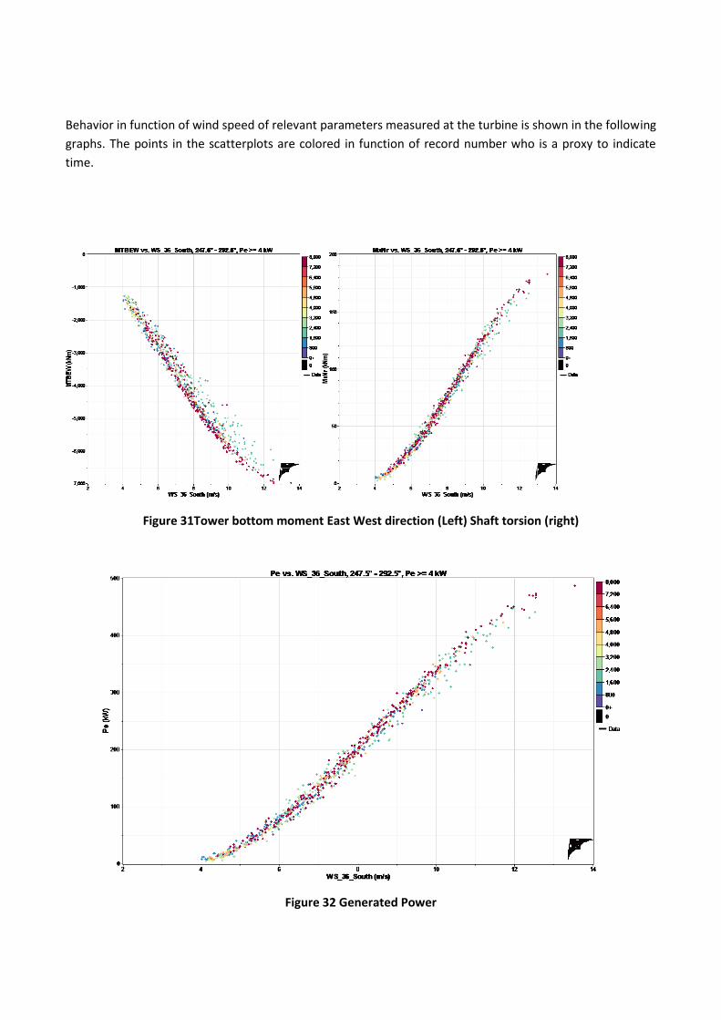
Behavior in function of wind speed of relevant parameters measured at the turbine is shown in the following

graphs. The points in the scatterplots are colored in function of record number who is a proxy to indicate

time.

Figure 31Tower bottom moment East West direction (Left) Shaft torsion (right)

Figure 32 Generated Power

Edgewise Flapwise

Bla

de1

Bla

de2

Bla

de3

Figure 33 Ten minutes averages of blade root bending moments versus wind speed

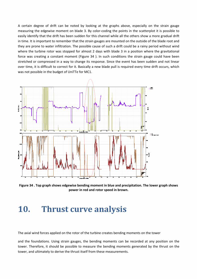
A certain degree of drift can be noted by looking at the graphs above, especially on the strain gauge

measuring the edgewise moment on blade 3. By color-coding the points in the scatterplot it is possible to

easily identify that the drift has been sudden for this channel while all the others show a more gradual drift

in time. It is important to remember that the strain gauges are mounted on the outside of the blade root and

they are prone to water infiltration. The possible cause of such a drift could be a rainy period without wind

where the turbine rotor was stopped for almost 2 days with blade 3 in a position where the gravitational

force was creating a constant moment (Figure 34 ). In such conditions the strain gauge could have been

stretched or compressed in a way to change its response. Since the event has been sudden and not linear

over time, it is difficult to correct for it. Basically a new blade pull is required every time drift occurs, which

was not possible in the budget of UniTTe for MC1.

Figure 34 . Top graph shows edgewise bending moment in blue and precipitation. The lower graph shows power in red and rotor speed in brown.

10. Thrust curve analysis

The axial wind forces applied on the rotor of the turbine creates bending moments on the tower

and the foundations. Using strain gauges, the bending moments can be recorded at any position on the

tower. Therefore, it should be possible to measure the bending moments generated by the thrust on the

tower, and ultimately to derive the thrust itself from these measurements.

The mass of the wind turbine contributes to the bending of the tower by applying a moment at

its top. This moment is roughly equal to the mass of the rotor multiplied by the shaft length (more precisely

to the distance between the rotor position, and the center of the tower), and by the gravity constant g.

The wind is also acting on the tower and is creating a corresponding bending moment at the tower bottom.

As the force is distributed over the section area of the tower, it is integrated to derive the bending moment.

The formula is therefore the integral of the force acting on an infinitesimal area of the tower multiplied by

the distance from the strain gauge. As the tower radius decreases significantly over the tower height (from

R0 to RHub), this is taken into account by assuming a linear decrease of the tower radius

Finally, the tilt moment of the turbine can also influence the bending moment measured on the tower. In fact, the difference of wind speed between the upper part and the lower part of the rotor can create a moment applied on the shaft at the connection with the rotor. This moment is propagated to the bottom of the tower where it is added up to the other contributions. This contribution is the smallest and is not considered in this analysis.

The thrust is only one component of various moments created by the complex interaction between the wind

flow field, the gravity field and the turbine. A model taking into account the major moments applied on the

tower is therefore needed to be able to derive the thrust from strain gauges measurements.

The model used is based on measurements of two strain gauges including information of wind direction, as

suggested in [7].

The meaning of the acronym explained in the following figure

Figure 35 Explanation of variables used in the model applied to derive thrust from strain gauges measurements.

By assuming small changes of wind direction in the 10 minutes period the formula above has been applied to

10 minutes averages go the values required. A scatterplot of 10 minutes values and bin averaged thrust in

function of wind speed can be seen in Figure 36 where it is compared to the thrust curve made available by

the turbine manufacture in wind resource assessment software. In this case WindPro.

Figure 36 Thurst in function of wind speed

References

[1] Measuring the inflow towards a Nordtank 500kW turbine using three short-range WindScanners and one

SpinnerLidar, (DTU Wind Energy E; No. 0093) Nikolas Angelou and Mikael Sjöholm, September 2015

[2]IMPER: Characterization of the Wind Field over a Large Wind Turbine Rotor : Final report. / Schmidt

Paulsen, Uwe; Wagner, Rozenn. Wind Energy Department, Technical University of Denmark, 2012. 335 p.

(DTU Wind Energy E; No. 0002). Research › Report – Annual report year: 2012

[3] IEC 61400-12-1 ed.1 Wind turbine power performance testing

[4] IEC 61400-12-1 Ed.2 Draft CDV

[5] IEC TS 61400-13 ed.1 Measurement of mechanical loads

[6] Demurtas, G., & Friis Pedersen, T. (2014). Summary of the steps involved in the calibration of a Spinner

anemometer. DTU Wind Energy. (DTU Wind Energy I; No. 0364).

[7] Pierre-Elouan RÉTHORÉ, s041541 “Thrust and wake of a wind turbine:Relationship and measurements”,

M.Sc. thesis, September 2006

Thanks to

All the TEM technicians who helped out setting up the experiment and performing all the required

verification.

unitte mc1 - nordtank measurement campaign (turbine and

Documents