1

Understanding Modern Portfolio Construction

Cullen O. Roche

February 22, 2016

ABSTRACT

Over the last 75 years there have been great strides in modern finance, portfolio

theory and asset allocation strategies. Despite this progress the process of portfolio

construction remains grounded in many theoretical concepts that can result in

inappropriate or unrealistic frameworks. In this paper we provide an overview of the

development of these ideas, construct a general foundation for understanding portfolio

construction and produce a framework for simplifying, systematizing and streamlining

the process in an attempt to establish a realistic and suitable process for portfolio

construction.

E-mail: cullenroche@orcamgroup.com

www.orcamgroup.com

2

Introduction

This paper introduces the basic historical background upon which modern finance

and asset allocation is implemented, provides a general understanding for portfolio

construction and offers some ideas for improving the methodology for Modern Portfolio

Construction (MPC).

This paper is organized in three sections. Section One discusses the historical

background of Modern Portfolio Theory (MPT) and how its influence resulted in many of

the ideas that dominate portfolio modeling today. Section Two discusses the general

building blocks of portfolio construction and how one should begin to approach the

process of asset allocation. Section Three builds on many of the positive developments in

MPT and modern finance and helps develop a realistic and practical framework for

Modern Portfolio Construction. We develop a general framework for understanding

portfolio construction and conclude that a low fee, tax efficient Countercyclical

Indexing™ strategy results in a rational and suitable approach to portfolio construction.

3

1. A Brief Review of Modern Portfolio Theory & Modern Finance

1952 marked the birth of Modern Portfolio Theory when Harry Markowitz

(Markowitz, 1952) developed his methodology of mean-variance optimization (MVO).i

Markowitz, widely recognized as the father of modern finance, established an approach

by which asset allocators could quantify how best to efficiently allocate assets by

measuring the degree of risk one takes in achieving a certain type of return.

Arguably, the most important development in the MPT framework (most notably

Markowitz 1959) was the development of a cohesive language and process for portfolio

construction. Several key concepts were derived from MPT including:

• The importance of understanding covariance and diversification as well as the

tendency for uncorrelated assets to create superior risk adjusted returns when

combined in a portfolio by reducing the total portfolio variance.

• The utilization of portfolio “risk” as standard deviation which helped develop

mathematical models for understanding risk in a portfolio.

• The development of the data driven concept of the Efficient Frontier which allows

asset allocators to create a systematic method for portfolio selection and risk

management.

MPT was a sufficient starting point for asset allocation models, but only laid the

theoretical foundation. The two most important developments in Modern Finance that

built on MPT included the Capital Asset Pricing Model (CAPM) and the Efficient Market

Hypothesis which is often commingled with the Fama French Factor Models.

The Capital Asset Pricing Model (CAPM) was developed by Jack Treynor,

William Sharpe, John Lintner and Jan Mossin in the 1960s.ii CAPM formalized a

framework by which asset allocators could understand the relationship between asset

returns and risk according to mean variance analysis. This mathematical model

distinguished between two specific types of market risk: 1) systematic risk (i.e.,

undiversifiable risk), and; 2) non-systematic risk (i.e., diversifiable risk). This asset

4

pricing model helped asset allocators distinguish between the returns generated from “the

market” (i.e., beta), and any excess return (i.e., alpha). According to CAPM there are

two ways to generate returns: 1) take the market return and; 2) beat the market. The

development of MPT and CAPM popularized the idea of using a market cap weighted

indexing portfolio as these methods emphasized the importance of a diversified market

portfolio. This era coincided with the significant growth in both beta replicators (index

funds) and excess return chasers (most active mutual funds).1

In 1976 Stephen Ross expanded on CAPM when he introduced Arbitrage Pricing

Theory (APT), which identified multiple sources of systematic risk.iii The crash of 1987

and the East Asian Currency Crisis increased focus on tail risk in portfolios and other

sources of market risk while diminishing the credibility of ideas like the Efficient Market

Hypothesis. These events resulted in greater research into market anomalies and

challenged the overly simplistic single factor approach like CAPM. These tail risk events

led to a widespread focus on Value at Risk models that use statistical properties to

calculate the worst case scenarios across portfolios. This increased the focus on hedging

strategies as well as the use of portfolio insurance such as options and futures contracts.

This era coincided with the significant growth in hedging strategies and hedge funds

specifically.

In 1992 Fama and French expanded on the Efficient Market Hypothesis with their

seminal research that identified three factors - market risk, value and size - to explain

market returns and helped build on APT as well as many of the weaknesses in CAPM.iv

Fama and French expanded on this model in 2014 when they added two new factors to

their three factor model. More recently researchers have added hundreds of different

factors.v As a whole, Factor Tilting has further expanded on a basic market cap weighted

approach by adding an increased degree of diversification through strategic asset

allocation. For instance, a market cap weighted stock portfolio might tilt to various

1 As Andrew Lo notes in “What is an Index” (2015) the concept of an “index fund” has changed substantially over time and now comprises a wide range of fund strategies that are trying to capture beta in various ways. In the modern world of low fee indexing there is an index for almost anything and everything.

5

factors such as the momentum and value factors which have shown a strong tendency to

outperform.vi

Increasing globalization and the unusually high correlations of financial assets

during the Great Financial Crisis led to the latest important developments in portfolio

theory. This era includes the rise of Smart Beta, Risk Parity, Tactical Asset Allocation,

Adaptive Asset Allocation and others. The Great Financial Crisis was particularly

influential because it exposed the weakness of a globally diversified portfolio and the fact

that, during a financial panic, all assets can become highly correlated. The tremendous

drawdowns in portfolios like a traditional 60/40 stock/bond allocation and the drawdowns

in most factors left asset allocators in search of a more suitable alternative which has

opened the door for alternative asset allocation strategies that question the way the

Efficient Market Hypothesis and Factor Investing approach risk and portfolio

construction. The more recent developments in portfolio theory focus increasingly on

how we define “risk” and how we develop fully diversified strategies.vii

The Great Financial Crisis also brought behavioral finance to the foreground as

economic theorists embraced the strong evidence of irrational behavior in both the real

economy and the financial markets. This brings us to the present day in which many of

these approaches are still being tested and critiqued by asset allocators.

The sum of these approaches has positively contributed to the way portfolio

construction is currently implemented. In particular, these developments have resulted in

several key improvements in the asset allocation process including:

1. The only “free lunch” in the asset allocation world is diversification.

2. The importance of low cost indexing due to the high cost of active management.

3. A consistent language and process for understanding the portfolio construction

process.

4. A greater understanding of the relationship between risk and reward.

Although these concepts have had a positive impact on the process of portfolio

construction over the last 75+ years asset allocators still struggle with their validity in the

6

process of identifying the optimal approach to the portfolio construction process. It is my

hope that these next two sections will provide further clarity to the discussion.

7

2. A Basic Framework for Understanding Modern Portfolio

Construction

Whether an asset allocator is an individual or an institution the process for asset

allocation is roughly the same:

1. Establish a well-defined set of financial goals.

2. Develop an appropriate understanding of “risk” as it relates to one’s risk profile. 2

3. Define the time horizon during which we are seeking to protect assets.

4. Acquire the appropriate assets that will create a high probability of matching our

risks, time horizons and financial goals.

5. Maintain this portfolio in order to ensure that our portfolios are consistent with

achieving our financial goals.

Before expanding on each of these topics in more detail we will construct a basic

understanding of the financial markets within the context of the modern monetary system

using a macro framework.

2.1 Thinking in a Macro Sense

This paper and its underlying concepts are all based on macro or aggregate

thinking. Before we dive into the meat of this paper we will first clarify some of the

issues regarding the common usage of some micro concepts that influence Modern

Portfolio Theory and the Efficient Market Hypothesis. As Paul Samuelson once said, the

market is “micro efficient”, but “macro inefficient”.viii It’s helpful to think of the markets

in a macro sense in order to avoid fallacies of composition. These fallacies include:

1. The false pursuit of alpha or “market beating” returns.

2. The dangers of relative returns and benchmarking.

3. Misunderstanding risk as the asset allocator perceives it as opposed to the way the

asset manager sees it.

2 The specifics of risk profiling require a great deal of customization depending on the individual or institution and will not be covered in general detail in this paper.

8

4. The false dichotomy of “active” and “passive” investing.

We will expand a bit on these fallacies in section 2.2 in order to provide further clarity for

our ensuing discussion.

2.2 The Arithmetic of Asset Allocation in a Global Financial World

At the aggregate level there is a single portfolio of all outstanding financial assets.3

This portfolio is highly dynamic, but in any given period these financial assets generate

“the market” return. This means that the holders of these financial assets must, by

definition, generate the post-tax and post-fee market return. The average asset allocator

will therefore generate the top line return from all outstanding financial assets minus any

taxes and fees paid. This means that, in the aggregate, no one “beats the market”.

Of course, some asset allocators must, by definition, outperform other asset

allocators inside of this aggregate portfolio. This creates a conundrum for the intelligent

asset allocator. Modern Portfolio Theory teaches us that diversification is the only free

lunch in asset allocation and that beating the market is extremely difficult for sustained

periods of time. And the arithmetic of asset allocation in a global financial world proves

that no one beats the market in the aggregate. Therefore, the intelligent asset allocator

must choose whether there is any relevance to the endeavor of trying to generate alpha or

excess return. This paper will argue that this is a false pursuit for, at the aggregate level,

there is no “alpha”, and there are only different types of beta.4

The primary reason why the intelligent asset allocator should avoid the pursuit of

excess return is that this is not an essential financial goal for most savers. While

generating high risk adjusted returns would be a nice benefit of intelligent asset allocation

3 We will refer to this aggregate portfolio as the “Global Financial Asset Portfolio” or GFAP. As we will discuss later, this portfolio is roughly outlined using the same framework as Doeswijk, Lam and Swinkels, 2014. 4 As an example of the difficulty of this, consider that a global portfolio of 50% stocks and 50% bonds has returned about 8.85% per year over the last 50 years. A taxpayer in the highest tax bracket paying the average asset management fee of 1% will reduce their compound annual growth rate to just 4.69% as a result of incurring short-term tax rates and high fees.

9

it is not necessary as part of a smart financial plan. Additionally, the intelligent asset

allocator understands the arithmetic of the global financial markets and how difficult it is

to consistently beat the market as evidenced by the annual SPIVA Scorecards.5

The false pursuit of alpha is problematic for other reasons as well. The result of this

pursuit of alpha leads asset managers to impose the way they perceive risk

(underperforming a false benchmark such as the S&P 500) on their customers. As Ben

Graham once said:

I could not comprehend how the management of money by institutions

had degenerated from the standpoint of sound investment to this rat

race of trying to get the highest possible return in the shortest period of

time. Those men gave me the impression of being prisoners to their own

operations rather than controlling them... They are promising

performance on the upside and the downside that is not practical to

achieve.ix

When the asset manager imposes his/her perception of risk on the customer he/she

is creating a conflict of interest since the risk to the customer is not benchmark

underperformance. The customer, after all, does not care if he/she beats the S&P 500 by 1

percentage point in a year like 2008 when asset prices fell nearly 50%; because he/she

has been exposed to a disturbing degree of permanent loss risk. The customer cares more

about generating a sufficient absolute return as opposed to a sufficient relative return. As

Charles Ellis (2014) notes, there has been a substantial change in the view of

performance investing; however, the size of the aggregate assets managed by more active

strategies still dwarfs passive strategies by 2:1.x, xi

The imposition of manager risk is compounded by the problem of benchmarking.

At the aggregate level there is only one true benchmark represented by the Global

Financial Asset Portfolio (GFAP). Anyone who deviates from this portfolio is essentially

making an active decision about their asset allocation. Since we all deviate from this

global cap weighted portfolio one could say that we are all “active” investors trying to

5 The 2015 SPIVA Scorecard by Standard & Poors showed that 75% of equity managers underperformed a correlated benchmark on a rolling 10 year basis.

10

obtain alpha, but simply trading beta. The intelligent asset allocator knows that alpha is

elusive in the long-run and will therefore embrace his/her deviation from market cap

weighting as an active asset allocator and accept the market return in an efficient manner

that has a high probability of helping achieve financial goals. Unfortunately, too many

asset allocators compare their returns to inappropriate relative benchmarks such as the

S&P 500 thereby compounding the alpha illusion and increasing the tendency to be

excessively active and behaviorally biased.

The construction of an aggregate global benchmark such as the GFAP exposes

some important understandings about the asset allocation process. One of the dominant

themes in asset allocation these days is the distinction between “active” and “passive”

investing. While this distinction was once quite clear it has become increasingly muddled

in a world in which most asset allocators have become asset pickers using low fee index

fund products instead of picking stocks. After all, a stock picker can be quite “passive”

(for example, Warren Buffet has a very low fee and inactive management style),

however, the stock picker is not merely trying to capture broad market returns. They are

trying to beat the market. This means that the most useful distinction between “active”

and “passive” is as follows:

Active Investing – an asset allocation strategy with high relative frictions that

attempts to “beat the market” return on a risk adjusted basis.

Passive Investing – an asset allocation strategy with low relative frictions that

attempts to take the market return on a risk adjusted basis.

This macro thinking highlights the fact that most asset allocators deviate from global cap

weighting and are therefore indirectly engaging in an effort to “beat the market” in an

active manner. As Cliff Asness of AQR has noted, one cannot deviate from global market

cap weighting and call themselves a “passive” investor:

11

You can believe your strategy works because you’re taking extra risk or because

others make mistakes, but if it deviates from cap weighting, you don’t get to call it

“passive” and, in turn, disparage “active” investing.xii

In this new age of macro indexing we are all essentially “asset pickers” operating in

differing degrees of allocation efficiency. The “active” versus “passive” distinction is

losing its relevance in a world where everyone can allocate assets in a low cost and

inactive manner using various forms of beta replicating instruments.6

Because the pursuit of alpha is often expensive (see hedge fund fees and after tax

returns or the high cost of chasing returnsxiii), the intelligent asset allocator will generate a

higher return by reducing these frictions as much as he or she can. As shown in Bogle

(2003), Barber (2000) & Vanguard (2014), taxes and fees are the most important

controllable frictions in portfolios. Therefore, the intelligent asset allocator should simply

try to “take the market return” as efficiently as possible while deviating from the GFAP

in a manner that is in-line with their risk profile.

These confusions regarding alpha, beta, active and passive stem largely from the

theoretical development of the EMH and CAPM. These theories continue to have a

tremendous impact on the way asset allocation is implemented even though their

limitations have been well documented, including:

• As Stiglitz (1980) notes, informational efficiency of markets is impossible.xiv

• As Bogle (2003) notes, it is not efficiency or inefficiency that matters, it is costs

that matter most.xv

• As Mandelbrot (1960) notes, these models lead to an insufficient focus on fat tail

events despite the fact that asset allocators are disproportionately concerned about

the risk of outlier events as evidenced in Thaler (2015) via the analysis of Myopic

Loss Aversion.xvi, xvii

6 The false dichotomy of “active” and “passive” can be best understood by understanding that passive investors need active investors in order to remain passive. That is, all index funds are, at their core, systematic actively managed products that require constant upkeep, changes and maintenance. E.g., the S&P 500 has had 320 deletions due to distress since 1980. Passive indexers pay active investors through bid/ask spreads, arbitrage costs and market making fees. In other words, there is no such thing as passive investing without active investing.

12

• As Montier (2013) notes, CAPM has severe deficiencies, the most important of

which is the exacerbation of the alpha obsession.xviii

These deficiencies are mostly micro model based limitations. We should

emphasize that these models are fine heuristic techniques even though they have

limitations. Asset allocators should understand these limitations when constructing

portfolios. By understanding these limitations and building on the benefits of this work

we can begin to formalize a more realistic and applicable model for Modern Portfolio

Construction (MPC).

2.3 Understanding Saving & Investment

We will be very precise about the terms saving and investing in this paper as these

terms are often misused in the fields of finance and economics. Confusion regarding

these topics can often lead one to engage in an asset allocation strategy that is

inappropriate. The following two definitions are simple, but important:

Investment - spending, not consumed, for future production.

Saving - income not consumed.

When we discuss investment we should be clear that most investment is done by

firms spending to produce goods and services. When a corporation builds a new factory

they are spending for future production. That is, they will create something that generates

more output in the future. Firms will sometimes finance this investment by issuing stocks

and bonds. The actual act of spending is investment, but we sometimes refer to the buyers

of these stocks and bonds as “investors” when the reality is that these investors have

merely reallocated their savings in order to finance investment spending.

For most of us, what we refer to as the act of “investing” is nothing more than a

reallocation of savings where we are purchasing stocks and bonds on a secondary market

in order to help us achieve some financial goal. This is essential to understand because

the act of investment is generally a very high risk endeavor that involves many more

13

corporate failures than successes. Reallocation of savings, however, is an act that is

generally synonymous with prudence and managed risk taking.

Further, the act of productive investment spending is generally positive sum as it

involves the creation of new potential future output. This is different from the act of

allocating one’s savings in already issued financial instruments that are valued based on

the efficiency of a firm’s investment spending and underlying operations. In other words,

an entrepreneur engaged in investment spending can create a positive sum outcome

whereas savers on a secondary market exchange instruments while taking financial

market returns.7 Savers revalue the size of the financial asset pool in the short-term based

on their best guess about underlying fundamentals whereas investors actually create the

fundamentals that make those financial asset returns sustainable in the long-run.

Thus, it is best to think of portfolio construction as the act of reallocating our

savings and this generally involves a lower risk and more prudent approach as opposed to

so much of the gambler’s mentality that we see in many of the corners of the financial

world today. Because we are discussing the process of savings allocation in this paper we

will refer to portfolios as “savings portfolios” and not “investment portfolios”.

2.4 Why do We Allocate Assets?

Before we can fully understand the process of portfolio construction we must build a

basic understanding of the financial world around us. The financial world exists as a tool

by which human beings can interact in the process of exchanging goods and services. In

order to streamline the process of exchange we have established a single fungible tool

that we refer to as money. As Roche (2011) notes, various financial instruments can serve

the primary purpose of money as a viable medium of exchange, but certain instruments

will always have a higher degree of moneyness than others in the modern monetary

7 Secondary markets are also positive sum in the aggregate because they are an extension of a growing pie of wealth over the long-term, however, asset allocators take the aggregate market return whereas entrepreneurs and investment spending can directly increase the size of the pie upon which market returns and their fundamentals are based.

14

system.xix When seeking to consume or spend for future production, one will try to

obtain a financial asset of high moneyness.8

Money is always and everywhere endogenous which means that anyone can create

money, however, as Hyman Minksy reminded us, although anyone can create money the

problem is in finding a willing holder of that money.xx As a result of this reality we find

that certain economic agents will create financial instruments with lower degrees of

moneyness that provide the holder of these assets with a greater sense of security. These

instruments are issued in order to compensate one for providing an instrument of higher

moneyness so that they can defer spending today with the prospect of being able to spend

more in the future.

The three most dominant forms of financial instruments include stocks, bonds and

cash.9 The first two of these instruments (stocks and bonds) are issued in order to acquire

liquid cash for the purpose of financing investment spending.10 Once issued these

instruments will trade on exchanges in the secondary market where savers reallocate their

holdings amongst one another.

Bonds are a type of debt issued in order to obtain something of higher moneyness

(such as cash) with the promise to repay the lender a greater sum in the future usually at a

fixed rate. Bonds are generally a more secure form of financial instrument as they contain

legal protections (such as seniority in the case of liquidation) and contractual obligations

(such as fixed temporal constraints regarding contractual lifetime and payments) that

make them a lower risk instrument relative to instruments such as stocks.

Equity, more commonly referred to as common stock, is another financial

instrument issued by firms seeking to obtain something of higher moneyness. Issuance of

8 “Moneyness” refers to the view that all financial assets exist on a scale of moneyness with cash equivalents having the highest degree of moneyness and other instruments such as bonds or stocks having lower degrees of moneyness. See Roche 2011 for more details. 9 “Cash” in this paper will be used in a broad sense and should not be taken to mean physical notes. Instead, “cash” comprises all physical notes and cash equivalents including short-term debt obligations and money market instruments. 10 “Stocks and bonds” includes market cap weighted aggregates such as the MSCI All World Stock Index and the Ishares Aggregate Bond Index. We exclude non-financial assets (such as commodities) and other more complex financial assets in this analysis for the purpose of simplicity.

15

common stock is generally a more expensive form of acquiring cash equivalents as it

requires that the owner of a firm relinquish some percentage of ownership. Stock is

inherently riskier as it is subordinate in the case of liquidations and has only loosely

defined contractual obligations regarding payments of income across time.

As previously mentioned, those of us on the secondary markets are merely

reallocators of savings. The primary purpose of this savings asset reallocation is to

protect cash equivalents from the loss of purchasing power. By owning cash equivalents

asset allocators will be protected from the risk of permanent loss, but will expose

themselves to a certain degree of purchasing power risk equal to the rate of inflation each

year. In order to protect one’s savings from the loss of purchasing power risk it is

generally wise to reallocate this savings into a diversified portfolio of stocks and bonds

that balance the risk of purchasing power protection with the exposure to the risk of

permanent loss.

2.5 What is Portfolio Risk?

In order to fully understand why we allocate our savings across various financial

assets it is important to understand what risk is and how it pertains to the financial asset

world. The idea of risk is a somewhat confusing and nebulous concept in modern finance.

The traditional textbook definition of “risk” is beta, standard deviation or volatility. This

is convenient for statistical purposes because it allows us to quantify risk when measuring

various outcomes. This definition, while useful in many ways, also has its limitations. For

instance:

1. Volatility isn’t always a bad thing. In fact, volatility with a positive skew is a

good thing. No one complains about a portfolio allocation that rises 20% per year

and falls 5% every once in a while, but this is a volatile position relative to many

portfolios.

2. Negative skew can be a good thing in a portfolio. For instance, many forms of

insurance have a natural negative skew and detract from returns, however, it

16

would be strange to argue that this is always a bad idea even if you don’t have to

use the insurance.

3. Asset allocators don’t live in a textbook world and don’t necessarily judge their

portfolios by the academic concepts that drive the way many portfolio managers

assess their portfolio performance. This can create inconsistency between the

asset allocator’s perception of risk management and the asset manager’s

perception of risk management.

For most asset allocators the “risk” of owning financial assets comes primarily from two

factors:

• Purchasing power risk.

• Permanent loss risk.

Purchasing power risk is the potential that one’s savings does not keep pace with the rate

of inflation. Permanent loss risk occurs when your savings is declining in value and one

is forced to take a permanent loss for some reason (emergency, behavioral, short-

termism, etc.). From these two basic understandings we can expand on the academic

notion of risk as beta and apply a more realistic framework:

Financial market risk is the probability of a loss of purchasing power and/or

permanent loss during an asset’s holding period.

In order to visualize how one might protect against these risks in a portfolio it’s helpful to

view this concept on a scale showing how our savings can be allocated across different

assets:

17

(Figure 1 – The Savings Portfolio Scale)11

The asset allocator who only wanted to be protected against permanent loss risk

might hold 100% cash; however, he/she would risk falling behind in purchasing power by

the rate of inflation each year. Likewise, the asset allocator who only wanted to

be protected against purchasing power risk would be 100% allocated to stocks since the

stock market has a consistent track record of outperforming the rate of inflation in the

long-term.

Stocks give the owner a claim on the profits that the underlying entity earns. This

generally means that the owner holds assets that give him/her a claim on the cost of

inflation (the cost of output) plus any profit premium. This will generally provide the

holder with an inflation protected asset as corporations earn the rate of inflation plus the

profit premium.12

Bonds, on the other hand, are a more secure income stream attached to the viability

of the issuing entity. While there is no guarantee of purchasing power protection high

11 For illustrative purposes only. 12 It is important to think of “stocks” as an aggregate within the context of this discussion. The “stock market” is comprised of entities that come and go, however, the “stock market” as a whole is a constantly evolving entity with a stream of profits that shuffles from firm to firm as the economy evolves.

18

quality bonds will tend to protect an asset allocator from the risk of permanent loss by

acting as a hedge relative to the equity piece. By allocating assets into a diversified

portfolio savers can maintain their purchasing power without creating unnecessary

uncertainty about potential future spending needs resulting from the potential of

permanent loss.

Importantly, you will notice that the Savings Portfolio Scale does not merely assess

the risks from stocks and bonds evenly. Instead, we have adjusted the scales to account

for the fact that permanent loss risk is skewed towards stocks. For instance, a 60/40

stock/bond portfolio’s exposure to permanent loss risk comes primarily from its 60%

stock component because this component determines over 85% of the total volatility in

the portfolio. Therefore, in periods such as the Great Financial Crisis a 60/40 portfolio

would expose the owner to 30%+ declines, creating a large degree of permanent loss risk

in the portfolio. Since stocks contribute such a high degree of permanent loss risk to

portfolios we must account for this when considering how “risky” our portfolios are.

2.6 Where Do Profits Come From?

To understand how we use various assets to achieve our financial goals, it helps to

understand why certain assets obtain the cash flows they do. In order to achieve this, it is

informative to understand where corporate profits come from, which requires a

macroeconomic understanding of the world. When we buy claims against firms, we are

buying a claim on a portion of their cash flows. Equities, for instance, provide the owner

with a claim on profits. Corporate debt provides the owner with access to a fixed

percentage of interest plus principal at maturity. But where do these cash flows come

from? The monetary system is the sum of all the transactions that occur within it. So we

know that profits come from a specific flow of funds. According to the Jerome Levy

Forecasting Center we can derive profits from a simple equation:

Profits = Investment–Household Savings–Government Savings

–Foreign Savings + Dividendsxxi

19

In short, profits come from business spending, household spending, government

spending, and foreign spending. This equation is expressed in Figure 2 as a percentage of

gross national product since 1960:

(Figure 2 – US Corporate Profits as % of GNP)

Figure 2 shows, as a percentage of GNP, the contributions to corporate profits from the

government deficit, net investment, dividends paid (“business” is dividends plus net

investment), personal saving, and the foreign sector. US households generally net save,

and the foreign sector has been in a current account deficit for most of the last fifty years,

so corporate profits have been driven mainly by net investment, dividends, and the

government deficit.

The problem, from an asset allocation perspective, is that corporate profits are

extremely cyclical and inconsistent. Figure 3 shows the year-over-year percentage change

in profits:

20

(Figure 3 – Year over year % Change in US Corporate Profits)

The figure demonstrates that profits are volatile and unpredictable. This results in a good

deal of uncertainty regarding the future expected value of the securities that are attached

to these profits. And this brings us to the problem of trying to assess what drives financial

instrument returns since they represent the market’s expectations as to the future expected

value of these instruments.

2.7 Where Do Financial Market Returns Come From?

Understanding the fundamental drivers of price changes has obvious limitations

since the financial markets reflect the expected future cash flows of unknown future

fundamentals. If we think of financial market prices as an extension of expected future

cash flows then price is little more than the incomplete information of the aggregate

markets. In other words, price is the equilibrium of liquidity where two willing parties

agree to disagree on the future expected value of an asset.13

In the long-run, the returns from the major asset classes are a function of the firm’s

profitability. As Ben Graham once said, however, the financial markets are a voting

machine in the short-term and a weighing machine in the long-term.xxii If we reduce our

13 “Agree to disagree” since, if both seller and buyer “agreed” on future fundamentals, they would not take the other side of the trade.

21

financial asset universe down to one firm with a static rate of income generation then this

entity can finance its operations from one of two external sources – it can issue debt and

it can issue equity. From the perspective of the issuing entity the cost of debt is relatively

low given that it creates a predictable and generally lower cost form of financing. This

provides the lender with a more stable, but lower type of return instrument. Most

importantly, debt contracts involve well defined and relatively short time horizons when

compared with equity. An aggregate bond index, for instance, has an average effective

duration of 5.5 years as of 2016.14 This means that the elasticity of the security price

relative to the gross rate of return is fairly low.

Equity, on the other hand, is the most expensive form of financing because it can

cost the owner a substantial unknown future value in the firm. Given the unpredictability

of future cash flows this also makes equity an inherently higher risk form of financing.

Hence, equity holders will demand a higher rate of return than bond holders. And unlike

their bond counterparts, equity does not have a well-defined time horizon.

Duration is particularly useful for understanding how to think of equity and debt

holdings inside of a portfolio. Although duration is a concept that is normally used to

estimate a bond’s sensitivity to interest rate risk we can also use this concept to

understand how stocks are sensitive to price changes. We can calculate the duration of

the stock market using the ratio of price to yield change, however, a more intuitive

concept is the break-even analysis for a set of probabilistic outcomes. Using this analysis

we arrive at an average equity market duration of 25 years.15

Asset allocators who hold equities are holding an inherently long duration asset and

demand to be compensated commensurately over the life of the instrument. Although

equity differs from debt we can derive the same basic understanding on equity returns as

we would with long bond maturities. That is, they command higher compensation in

order to offset the risk that their money might not finance an equal or greater quantity of

future spending.

14 This is in reference to the average duration of the Core US Aggregate Bond Market. 15 We can construct a basic scenario analysis to stress test the portfolio’s exposure to negative price shocks. In this case we use the current dividend yield of ~2% on the S&P 500 relative to the break-even prices on a range of declines from -25% to -75% assuming no change in dividends (a fair estimate given the stability of historical rolling 20 year dividend payouts). This heuristic technique is imperfect, but as a general guide it is a good approximation of the duration of corporate equities.

22

Understanding relative durations can be useful to understand in asset allocation

since our financial timeframes are often shorter than the lifetimes of the instruments we

own. Most asset allocators, for instance, do not have a realistic 25 year time horizon and

must balance their exposure between stocks, bonds and cash accordingly. Understanding

why certain financial instruments generate returns and applying an appropriate time

horizon to your asset allocation choices will be crucial to building portfolios that match

your risk profile.

2.8 The Intertemporal Conundrum & Asset Allocation

Asset allocation is ultimately about matching the proper duration of certain

financial assets with our financial goals. We want to be able to protect our assets from the

time decay of inflation without exposing those assets to the uncertainty that comes with

the risk of permanent loss. You could say that portfolio management is really time

management. Unfortunately, the concept of time in a portfolio is necessarily vague

because the instruments we utilize have uncertain future cash flow streams and we’re

attempting to match those instruments to an uncertain financial future.

Asset allocation necessarily involves the problem of asset and liability mismatch.

That is, we have certain outlays and liabilities that require financing over time. We must

balance the way we protect our financial assets from risk with the way that we create

certainty around our spending needs. This intertemporal conundrum is central to

understanding asset allocation.

Because our financial lives are filled with uncertainty and inconsistent spending

needs we must be careful with ideas such as “stocks for the long-run”. After all, most

savers don’t have a time horizon that corresponds to the “long-run” as most of our

spending needs occur continuously across the duration of our lives. Exposing our savings

entirely to the volatility of the stock market will substantially increase the risk of

permanent loss as asset allocators find themselves exposed to the potential for necessary

outlays at inopportune times.

23

At the same time, we should be wary of the excessive short-termism in the

financial markets these days. When we buy stocks and bonds we are dealing with

instruments that can range from very short-term (e.g., T-Bills) to very long-term (e.g.,

stocks or 30 year T-Bonds). Even a standard “Balanced Index” like a 60/40 stock/bond

index has an average duration of roughly 17 years. Judging the performance of this

portfolio on anything less than a multi-year rolling basis is irrational and likely to be

counterproductive.

As a simple rule of thumb it can be helpful to utilize the aforementioned concept of

duration when stocks have a very long duration (in this case 25 years) and bonds have a

much shorter duration (in this case 5.5 years). As an example, a 45 year old asset

allocator with 20 years to retirement might implement a rule such as the following:

PD=(S*25) + (B*5.5)

Where PD = Portfolio Duration, S = % stock allocation & B = % bond allocation.

In this specific case, our Portfolio Duration is 20 years and therefore our stock

allocation would be 75% and our bond allocation would be 25% [~20 =

(0.75*25)+(0.25*5.5)]. The asset allocator would readjust and rebalance this portfolio

annually to account for the changes in duration over time, i.e., shortening the duration

with each passing time period. Figure 4 provides a simplified cheat sheet for the current

environment:

(Figure 4 – Approximate Asset Allocations Based on Portfolio Duration)

Some asset allocators might argue that this approach is excessively conservative

given the long time horizons in some periods; however, we would argue that this

24

approach is more consistent with the views of a “savings portfolio” as well as the risks

assessed in the Savings Portfolio Scale where an excess amount of permanent loss risk

comes from the equity component. And while history has shown that stocks typically

perform well in the long-run, evidence has shown that there are potential risks in relying

on such assumptions.xxiii

2.9 Asset Allocation in a Global Financial System

Thus far, we have highlighted several key points in Modern Portfolio Construction

including:

• How a macro perspective will help us avoid the many fallacies of composition

that can mislead asset allocators.

• Taxes and fees are the most important controllable frictions in our portfolios.

• Diversification is the only free lunch in asset allocation.

• Financial market risk is the probability of a loss of purchasing power and/or

permanent loss during an asset’s holding period.

• The Intertemporal Conundrum highlights the importance of asset/liability

mismatch and the necessity to create certainty within an uncertain set of financial

circumstances.

Within this context we will expand on these concepts in the scope of the global financial

markets. The optimal way to construct a diversified Savings Portfolio in a tax and fee

efficient manner is through the use of index funds inside of a global asset allocation.

Indexing highlights several key points:

• As Bogle (2003) notes in his Cost Matters Hypothesis, a low cost indexing

strategy is consistent with higher average returns.xxiv

• As Barber & Odean (2000) highlights, trading and excessive activity is generally

consistent with lower average returns.xxv

• As Burns (2004) and Vanguard (2014) show, index funds are not merely average,

but actually outperform the majority of more active alternatives.xxvi, xxvii

25

• Asness (2011) and Vanguard (2006) show that a globally allocated portfolio can

improve overall diversification by reducing exposure to home bias and economy

specific risks.xxviii

These views are consistent with an approach that is similar to the Global Financial Asset

Portfolio which we will expand on in Section 3.

2.10 The Importance of Maintenance and Process

The portfolio construction process does not end once an asset allocator has

constructed his or her initial asset allocation. In order to ensure that a portfolio remains

in-line with its stated financial goals it will be important to maintain the portfolio over

time. The three keys to this process include:

• Rebalancing & contributing to a portfolio to remain in-line with the risk tolerance.

• Tax efficient maintenance.

• Fee efficient maintenance.

We will expand a bit on each of these below.

Rebalancing involves the practice of updating a portfolio allocation so that it

remains in-line with your financial goals. The primary purpose of rebalancing is to offset

the procyclicality of the stock portion of a portfolio. For instance, between 1972 and 2015

a portfolio of 50% US stocks and 50% US bonds grew at a compound annual rate of

9.1%. If one had not rebalanced this portfolio the allocation would have grown into a

77% stock and 23% bond portfolio due to the outperformance of the stock component.

As a result of this the portfolio exposed the asset allocator to greater permanent loss risk

as it evolved. For instance, the maximum calendar year drawdown of the unbalanced

portfolio was over 25% during the Great Financial Crisis whereas a rebalanced portfolio

declined by just 17% during the same period. Interestingly, by rebalancing the portfolio

one generated almost the exact same nominal return without exposing the portfolio to the

higher degree of permanent loss risk during the Great Financial Crisis. This has been

referred to as the “rebalancing bonus” by William Bernstein.xxix

Rebalancing is essentially a form of active management; however, we would like

to stress the fact that this should not be confused with the pursuit of market beating

returns. Instead, rebalancing should be thought of as risk profile maintenance. If the

26

rebalancing bonus persists then this is simply a pleasant surprise, however, we do not

rebalance in order to pursue alpha. We rebalance in order to maintain our risk profile.

In addition to rebalancing, we should be mindful of consistently feeding our

portfolios with fresh savings contributions. Reinvesting dividends earned and

contributing new savings to the portfolio is important to a systematic savings plan as this

can help to reduce your portfolio duration thereby reducing the asset/liability mismatch

uncertainty. In other words, the best way to reduce your portfolio’s break-even point is to

contribute new capital at current prices regardless of market performance.16 In addition,

new capital contributions help to compound future returns while creating optionality in

the portfolio.

Considering that rebalancing and contributing requires some degree of activity, we

should be mindful of taxes and fees inside of these forms of maintenance. Vanguard

(2015) finds that there is no material difference between monthly, quarterly and annual

risk adjusted rebalancing returns; however, there are substantial frictions incurred by

more frequent rebalancing.xxx Rebalancing strategies will be unique to each portfolio

given differing financial goals and allocations. Although there is no universal rule for

rebalancing, it is prudent to maintain a reasonably long rebalancing time frame of 366

days so as to minimize capital gains and costs. As a simple rule, annual maintenance is

consistent with a tax efficient and low fee management style.

When we look at portfolio returns it is important to understand “real, real returns”.

This is the post-inflation and post-friction return that one earns. This is the amount that

actually goes into your pocket and can be applied to future purchasing power. Although

we can’t control the markets or the rate of inflation we can control the two largest

frictions in our portfolios – taxes and fees.

As of 2016 the average investment manager fee was 1% of assets per year. If we

assume a $100,000 starting balance growing at 7% per year this 1% fee will cost the asset

allocator more than $15,500 over the next 10 years versus the option of a low fee index

costing 0.1%. Not only is the fee expensive in nominal terms, but it is compounded by

the fact that it reduces the balance in your account that could also be compounding

16 Capital contributions reduce duration by shortening the break-even point. Since yield impacts duration the compounding effect from higher account balances is positively skewed by capital contributions thereby reducing overall duration.

27

growth. In this sense, high fees act as a double tax on the portfolio. Paying low fees via

the use of index funds and ETFs is important when we know the pursuit of alpha doesn’t

generally pay off.

The lesser discussed, but also important portfolio friction is the “Uncle Sam”

friction (i.e., taxes). For a taxpayer in the highest tax bracket of 39.6% in 2016 the

difference between paying ordinary income tax rates on capital gains versus long-term

capital gains rates of 20% will result in the asset allocator foregoing 4% of their total

return over a 10 year period assuming a 7% compound growth rate. The cost of taxes and

fees helps explain why most active mutual funds can’t outperform their lower fee and

more tax efficient indexing counterparts.xxxi

28

3. Building on Recent Developments in Modern Finance

One of the dominant trends resulting from Modern Portfolio Theory is the

tremendous growth in Exchange Traded Funds (ETFs) and index funds. These

diversified products have become the fastest growing segments of the asset management

business as evidence has mounted that lesser diversified and more active strategies do not

fare well in comparison. This transition in the asset allocation world has coincided with a

substantial change in the way portfolio construction occurs.

In an effort to rectify some of the short-comings of MPT, the traditional market cap

weighted portfolio representing the broader markets has been expanded on and

challenged by approaches such as Factor Investing, Smart Beta, Risk Parity and others.

The Great Financial Crisis exposed certain flaws in the market cap weighted approach

leaving many asset allocators in search of an alternative. This next section will discuss

the development of some of these ideas as well as the rationale for a Countercyclical

Indexing strategy.

3.1 Assessing the Utility of the Global Financial Asset Portfolio

A tremendous amount of energy has been spent developing and identifying

superior asset allocation models over the last 75 years. Despite this effort there remains a

considerable disagreement about the ideal way to develop and maintain savings

portfolios. Historically, this battle for portfolio optimality has fallen between two camps

– the “active” and “passive” asset allocators. The active asset allocators argue that one

should try to identify market inefficiencies and actively take advantage of the market’s

errors while the passive asset allocator argues that the market is largely efficient and one

should therefore accept what the market offers.

We have already shown why this dichotomy can be misleading when all asset

allocators deviate from global cap weighting and have access to low cost index funds.

Importantly, we should emphasize that it isn’t difficult to outperform “the market”

29

because it is either efficient or inefficient. It is difficult to outperform due to the

arithmetic of the financial markets and the resulting high costs of active management.

In order to build a better understanding of a logical portfolio construction starting

point we will further explore the Global Financial Asset Portfolio (GFAP), the one true

benchmark. After all, the asset allocator who assumes markets are efficient and wants to

“take the market return” while avoiding any active deviations from global cap weighting

would simply buy this aggregate portfolio in a simple low cost form. As William Sharpe

noted in 2014, an ideal “market” index would reflect the current state of the GFAP:

I would like to see a very-low-cost index fund that buys proportionate shares of

all the traded stocks and bonds in the world. Unfortunately, there are none at

present.xxxii

Doeswijk, Lam and Swinkels (2014) provides a good approximation of what a

comprehensive “index” or global “market” portfolio might look like:xxxiii

(Figure 5 – The Global Financial Asset Portfolio)

This paper updates the GFAP as of 2016 to note recent changes as well as some

simplifications in the portfolio that make it more applicable in the real-world.

30

Specifically, we construct the portfolio using the two dominant asset classes (stocks and

bonds) and limit the portfolio only to financial assets so as to avoid unnecessary

complications that can arise from the use of non-financial assets.17 Using data from

World Exchanges and the BIS we find the current breakdown:

(Figure 6 - The Four Fund Global Financial Asset Portfolio)

This portfolio is particularly useful as a global benchmark for the following reasons:

1. It is a good approximation of the current global market cap weighted portfolio.

2. It can be easily implemented in a low fee and tax efficient manner using just 3 or

4 ETFs or Index Funds.

3. It removes asset class overlap and confusion by reducing the portfolio to financial

assets.

4. Annual maintenance can be systematic and simple.

If we assume that the markets are efficient and that lower frictions will result in

better returns, then an indexing strategy that reflects the GFAP should be highly useful.

On the other hand, assessing this portfolio is illuminating because it highlights many of

the rationalizations for a more active deviation from global cap weighting.

The gold standard for asset allocation benchmarks in recent decades has become

the 60/40 balanced index. This low fee and tax efficient index reflects a broadly

17 Non-financial assets refer to any tangible or intangible asset for which no corresponding liability is recorded. Potential non-financial asset complications include low real returns, categorization & liquidity.

31

diversified portfolio usually comprised of US stocks and US bonds. Most active

managers have lagged this simple index over its history and a review of the GFAP’s

returns shows that it too has failed to outperform the 60/40 index. Since 1959 the 60/40

index has generated historical compound annual returns of 9.61% with a standard

deviation of 10.9, a Sharpe ratio of 0.58 and a Sortino ratio of 0.81, while the GFAP has

generated just a 8.86% compound annual growth rate (CAGR) with a standard deviation

of 9.99, a Sharpe Ratio of 0.55 and Sortino Ratio of 0.78. In other words, the GFAP has

failed to outperform a domestically tilted 60/40 in both nominal and risk adjusted terms.

These findings add credence to Samuelson’s Dictum that the markets are “micro

efficient,” but not “macro efficient”. In other words, even the most basic deviation from

“the market” portfolio has proven beneficial.18

Even more interesting than the 60/40 portfolio is the inverted GFAP. If one were to

take the market cap weightings of the GFAP going back to 1959 and invert the stock

relative to bond weightings they would have generated better nominal and risk adjusted

returns. The standard market cap weighted GFAP generated CAGR of 8.86% at a

standard deviation of 9.99 with a maximum calendar year drawdown of -20% while the

inverted GFAP would have generated a 9.41% CAGR at standard deviation of just 8.9

with a maximum calendar year drawdown of -15.4%. In other words, betting against “the

market” portfolio proved beneficial over this time period. There are a number of possible

explanations for this unexpected outcome:

1. Using an ex-post snapshot of the financial markets might not be ideal given that

the current markets reflect the way in which capital allocators perceive the current

state of the financial markets, interest rates and future risks.

2. A market cap weighted asset allocation largely reflects the procyclical trends of

capital raising needs of underlying entities and could be unduly influenced by the

current structure of interest rates. As a result, when interest rates are high, capital

markets might prefer to issue equity relative to debt in which case the balance of

overall equity might expand relative to debt balances. As a result, the capital

markets could be overweight equities at a time when bonds are much more

18 Due to the lack of a global bond index and the skew of the 1980-2015 bond bull market we used T-Bond returns going back to 1959 relative to US stocks.

32

attractive to savers, as was the case in the early 1980s when the GFAP portfolio

was substantially overweight equities prior to the greatest bond bull market in

history.

3. The GFAP treats all bonds as being equal despite the fact that domestic US bonds

have outperformed foreign bonds historically on both a nominal and risk adjusted

basis. This could be explained by the USA’s unique standing in the world as both

the largest economy and the issuer of the world’s safe haven financial asset, US

Treasury Bonds.

Based on these findings, the GFAP, while adequate, could prove to be a suboptimal

portfolio at times. This is particularly true when considering the necessity of

personalizing a risk profile with the understanding that the GFAP will not be appropriate

for all asset allocators. Therefore, it could be wise to consider alternative asset allocation

strategies within the context of a low fee and tax efficient framework.

3.2 The Rationale for a Countercyclical Indexing Approach

In this section we will explain the rationale for a Countercyclical Indexing strategy

showing the following:

• A Countercyclical Indexing strategy can be implemented in a tax and fee efficient

manner in a globally diversified portfolio.

• A Countercyclical Indexing strategy can be implemented in a fully systematic

approach thereby removing discretion and creating an indexed strategy.

• A Countercyclical Indexing strategy will better align the risk profile of the asset

allocator with how he/she actually perceives risk through the market cycle,

thereby reducing the behavioral risk of loss aversion and imbalanced exposure to

permanent loss risk.

• We can remove manager risk by eliminating the search for alpha and instead

seeking to take the market return in a manner that is consistent with the way most

asset allocators perceive risk as opposed to the imposition of manager risk that

conflicts so many asset managers.

33

The GFAP and a basic 60/40 stock/bond portfolio are excellent portfolio options

when utilized in a low fee and tax efficient approach. There is a strong likelihood that

higher fee and more active managers will have a very difficult time outperforming these

strategies. While the GFAP and the 60/40 are useful as a starting point they could prove

suboptimal relative to low fee alternative indexing approaches. In order to resolve some

of the flaws in the GFAP and 60/40 index we will propose a systematic, low fee and tax

efficient indexing strategy called Countercyclical Indexing.

The use of systematic countercyclical policy is commonplace in macroeconomics;

however, it is not commonly associated with portfolio construction. In terms of

macroeconomics, the most common form of countercyclical policy involves what are

called “automatic stabilizers”. Automatic stabilizers involve the systematic expansion and

contraction of the government’s budget deficit/surplus in order to offset the current state

of the economy. This generally means that tax receipts are automatically increasing

during economic expansions and declining during contractions while government

spending is also automatically contracting during expansions and expanding during

contractions (e.g., due to increases in unemployment claims). The result of this is an

automatic countercyclical policy response in the size of the budget deficit/surplus which

adds income and net financial assets to the private sector during contractions while

reducing income and net financial assets during expansions. This automatic

countercyclical policy measure acts as a non-discretionary buffer to economic shocks.

Modern indexing strategies tend to result in static and/or procyclical portfolios. For

instance, the 60/40 balanced index is an inherently procyclical portfolio due to the fact

that its risk weighting is so heavily skewed by the stock market. Therefore, the asset

allocator who owns the 60/40 index will tend to be overweight equities when they are

most risky. This is due to the fact that equities have dynamic risk exposure and can

become more risky as they rise in value and can become less risky as they decline in

value. The result of the 60/40’s risk exposure is a relatively imbalanced exposure to

permanent loss risk. For instance, the 60/40 index exposed asset allocators to over 30%

declines during the Great Financial Crisis. This is testing the behavioral limits of the asset

34

allocator who believes they own a “balanced” exposure to the financial markets. Indeed,

they own a highly imbalanced exposure as the 60/40 portfolio will generate almost 70%

of the negative volatility of the S&P 500 while maintaining a high overall correlation

with the broader stock market. This is due to the fact that the 60% equity allocation

dominates the portfolio’s exposure to permanent loss risk in the short-term.

Several strategies have been designed to offset some of these flaws including Risk

Parity, Smart Beta and some combinations of Factor Investing; however, none are

implemented in fully systematic countercyclical strategies. For instance, some Smart Beta

strategies will take a market cap weighted equity index and weight the holdings as an

equal weighting thereby attempting to reduce the exposure to the most procyclical

holdings in the market cap weighted portfolio. However, these strategies require a more

fully uncorrelated diversifying strategy or asset class in order to offset the fact that even

an equal weight equity portfolio, on its own, will remain highly procyclical due to its

high degree of equity exposure.

Factor Investing, while showing strong empirical backtested results shows less

conclusive real-time results. This is largely due to the fact that factors are often easy to

identify in retrospect, but more difficult to identify in advance.19 As a result, there is not

conclusive evidence, as evidenced by Idzorek (2013) that a Factor Tilting portfolio will

consistently outperform a market cap weighted portfolio on an after tax and fee basis.xxxiv

Further, McLean (2015) shows that once factors are publicly identified they tend to lose

their significance.xxxv We must note that we are intrigued by the persistence of the value

and momentum factors when combined, however, this ultimately suffers from the same

pitfall as Smart Beta as the asset allocator must still combine a sufficiently uncorrelated

asset class to offset the procyclical tendency of the momentum and value stocks. In other

words, even if one could perfectly identify momentum and value in advance (an assertion

we find highly questionable), these equity instruments will tend to have a high degree of

procyclicality due to their high correlation with broader equity markets.

19 Factor investing relies on the ability of a passive manager to define a set of criteria for a fund that will consistently identify these factors in advance. We would call this a more micro form of asset picking inside of the GFAP and question the evidence that this can be consistently achieved in the real world.

35

Rebalancing is perhaps the most common form of a countercyclical measure in that

the asset allocator is systematically reducing exposure to equity across time. For instance,

a 60/40 will tend to grow into a 70/30 over time thereby exposing the asset allocator to

increased equity market risk. By rebalancing systematically the asset allocator can reduce

equity market risk, however, we would argue that rebalancing strategies are insufficient

on their own due to the fact that equities will still expose the asset allocator to excessive

permanent loss risk at the times when equities are most risky. In other words, rebalancing

back to a 60% equity weighting does not always expose the portfolio to the same degree

of risk since the 60% equity piece has an inherently procyclical and dynamic risk

exposure.

Our Countercyclical Indexing methodology is most influenced by the Risk Parity

research by Ray Dalio (2010) and William Sharpe’s Adaptive Asset Allocation Policies

(2009). Dalio’s Risk Parity approach has been instrumental in redefining the appropriate

way to assess and measure risk exposures in a portfolio.xxxvi Using a dynamic concept of

risk across time the Risk Parity approach seeks to create balance in a portfolio by

measuring the way in which assets expose the portfolio to risk. As an oversimplified

example, understanding that equity exposes the 60/40 index to excess permanent loss

risk, one might leverage the bond piece to further hedge the equity component’s greater

permanent loss exposure. Unfortunately, Risk Parity has its own limitations including a

high degree of forecasting error, generally high fees, high tax cost ratios and the use of

leverage.xxxvii

William Sharpe’s Adaptive Asset Allocation is more intuitively appealing and

consistent with our overall methodology.xxxviii Sharpe shows that a portfolio like the

GFAP or 60/40 index is dynamic and that an asset allocator would be wise to account for

the way the market cap weighted portfolio adapts over time. Therefore, Sharpe

recommends a rebalancing methodology whereby the asset allocator alters the subsequent

weightings to account for changes in the broader financial markets. This adaptive

rebalancing methodology makes a great deal of sense; however, it doesn’t resolve the

problem that Risk Parity portfolios are attempting to resolve – the inherent imbalance

between asset class risk exposures.

36

3.3 Resolving the Problem of Inherent Procyclical Risk

The intelligent asset allocator will try to balance his/her exposure to permanent loss

risk with the way he/she protects against the risk of purchasing power loss. The problem

with these risk exposures is that they are not static. There will be times when the equity

markets expose an asset allocator to low levels of permanent loss risk, and higher levels

of permanent loss risk due to the equity market’s inherent tendency to be procyclical

relative to other assets. This problem is compounded at times by the fact that any

portfolio that is overweight equities is insufficiently hedged since the equity piece

exposes the portfolio to a higher degree of permanent loss risk.

In order to understand this cause and effect it’s helpful to look at the underlying

drivers of price and fundamentals in the financial markets. When the financial markets

boom and bust across time these deviations tend to be the result of financial imbalances.

For instance, when financial markets priced-in very high technology stock prices in the

late 1990’s they were pulling future potential returns into the present while financing a

higher portion of investment spending with new equity issuance. This creates what can be

thought of as a price compression where future cash flows are being priced into the

present. What happens as a result of this change is that the equity market, as a relative

percentage of the cash and bond markets expands. These changes can be seen in the

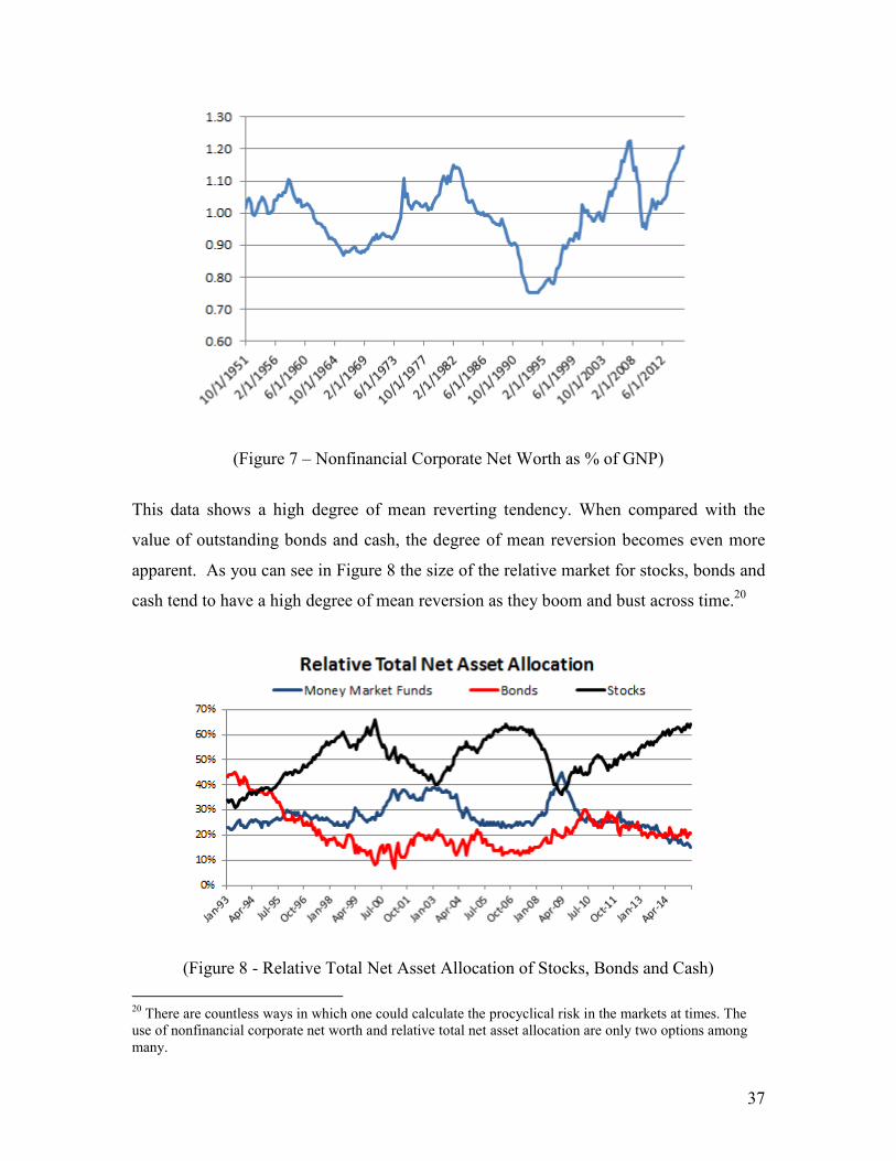
historical value of nonfinancial corporate net worth relative to GNP:

37

(Figure 7 – Nonfinancial Corporate Net Worth as % of GNP)

This data shows a high degree of mean reverting tendency. When compared with the

value of outstanding bonds and cash, the degree of mean reversion becomes even more

apparent. As you can see in Figure 8 the size of the relative market for stocks, bonds and

cash tend to have a high degree of mean reversion as they boom and bust across time.20

(Figure 8 - Relative Total Net Asset Allocation of Stocks, Bonds and Cash)

20 There are countless ways in which one could calculate the procyclical risk in the markets at times. The use of nonfinancial corporate net worth and relative total net asset allocation are only two options among many.

38

Of course, this makes intuitive sense since the stock market tends to become a

larger piece of aggregate financial assets late in a market cycle and tends to shrink

relative to aggregate financial assets during contractions. As the stock market pulls

returns into the present it is increasing its potential exposure to future permanent loss risk

whereas, during downturns, the exact opposite is occurring.21

The cause of this boom/bust phenomena is debated, but very likely has to do with

the behavioral biases of asset allocators and financial asset issuers and their tendency to

chase returns late in a cycle and shun riskier assets as they decline in value. But this also

has fundamental intuitive reasoning as well. As the economic cycle progresses the boom

pulls returns into the present thereby creating a potential imbalance in future returns.

Additionally, as equity prices rise the replacement cost of capital also tends to rise

at the times in the market cycle when entrepreneurs are trying to finance investment

spending with more and more equity issuance. And since equity cannot become 100% of

the aggregate financial asset pie (just as cash and bonds cannot become 100% of the

aggregate financial asset pie) there will tend to be a high degree of relative asset price

mean reversion across time. As a result of this, equity tends to become a larger and riskier

piece of the aggregate financial asset pool during expansions while equity often becomes

a smaller and less risky piece of the aggregate financial pool during contractions.

This thinking is not only intuitively appealing, but is consistent with empirical

research on value investing. As GMO (2015) notes, a focus on value over cycles can

dampen drawdowns.xxxix However, we would again emphasize that this type of factor

based approach on its own is insufficient. You must implement the use of a sufficiently

uncorrelated asset class relative to the equity piece. Within this context the use of a bond

market hedge in the form of an aggregate index can be useful, however, we might even

emphasize deviating from this portfolio as a bond aggregate will tend to provide less

permanent loss risk than a longer dated Treasury Bond portfolio during times of financial

21 It can be useful to again think of stocks as bonds in this example. For instance, a T-Bill yielding 3% will sell at $97.09 and mature at par in one year. If rates were to move instantaneously higher to 6% the price of this bill will decline to $94.34 for an unrealized 2.83% loss. If one were to buy this bill after the decline the yield to maturity will increase to 5.99% thereby resulting in higher returns. In other words, future returns were pulled into the present as the asset’s price declined. The inverse can occur during a bull market.

39

panic due to the unique positioning of the US government in the current global monetary

system as the issuer of the world’s highest quality debt instruments.xl One could also

argue that deviations from a bond aggregate makes sense in a world of persistent QE

where “the market” portfolio has been substantially altered by government policy,

however, this paper has neither the space nor scope to cover such a topic.

Our research shows some very promising results that confirm the concepts

discussed in this paper. Specifically, we find that a Countercyclical Indexing strategy that

inverts the current relative total asset allocations creates a sufficient return that is more

consistent with how most asset allocators perceive risk primarily because the portfolio

does not expose the asset allocator to a large degree of permanent loss risk at times when

the equity component is exposing the asset allocator to the highest degree of procyclical

permanent loss risk. By inverting the relative stock and bond weightings we find that a

globally allocated Countercyclical Indexing strategy generates superior risk adjusted

returns than a globally allocated 60/40 stock/bond portfolio while exposing the asset

allocator to smaller maximum drawdowns:

(Figure 9 – Countercyclical Indexing Portfolio Performance)22

What’s equally informative about this systematic Countercyclical Indexing

approach is that we can implement substantial out-of-sample testing of the approach since

we have over 70 years of publicly available data with which to apply to certain

allocations. For instance, because the portfolio tends to be bond heavy at times we might

be concerned about the performance during a rising interest rate environment. Since we

can test data going back to 1952 we are able to test this strategy performance during the

sharp interest rate increases from 1952-1980. We found that the Countercyclical Indexing

22 We used the 35 year period starting in 1990 in an attempt to create a fully representative global allocation with a reliable emerging markets index using the MSCI Emerging Markets Index.

40

strategy using a simple domestic allocation of stocks and bonds generated 8.32% CAGR

with a standard deviation of 10.86.23 This was largely in-line with the 60/40 index which

generated 8.38% CAGR with a standard deviation of 11. What’s interesting to note,

however, is that the Countercyclical Indexing portfolio matches the 60/40 index’s

performance during turbulent bond market environments (the pre-1980 period) and

outperforms it during substantial stock market turbulence (the post-1990 period). In the

aggregate, since we are not engaging in forecasting whether there will be future stock or

bond market turbulence the Countercyclical Indexing strategy represents an attractive

alternative to the 60/40 index since it reduces the asset allocator’s exposure to permanent

loss risk during periods of stock market turbulence.

The Countercyclical Indexing methodology is appealing for several reasons:

• This strategy aligns well with the concept of the Savings Portfolio since it

matches a certain asset allocator’s risk profile so as to adequately protect against

permanent loss risk and purchasing power risk.

• This style of indexing strategy can be implemented in a low fee and tax efficient

manner that essentially reflects a practical form of rebalancing or Adaptive Asset

Allocation as defined by William Sharpe.

• This strategy reflects an index since it can be implemented in a fully systematic

manner so as to avoid forecasting risk, asset manager discretion and potential

manager conflicts.

• Because the portfolio has a natural countercyclical element it will buffer against

the behavioral tendency to chase returns and sell into downturns. As a result, this

strategy reduces the potential negative risk of loss aversion in addition to other

common behavioral risks.

• There is strong macroeconomic evidence that countercyclical policy is beneficial

and this portfolio management strategy creates a consistent macro framework

across both macroeconomics and macro finance.

23 We used T-Bonds and US stocks in these calculations due to a lack of reliable international datasets.

41

Conclusion & Implications for the Financial Industry

We have emphasized several key points in this paper including:

• The importance of maintaining a globally indexed savings portfolio.

• The importance of a low fee and tax efficient approach.

• The superiority of index funds and ETFs relative to more active and lesser

diversified alternatives.

• Properly understanding the concept of risk and applying it in an appropriate

manner relative to your financial needs and goals.

• The avoidance of the pursuit of alpha as a financial goal and the limitations of the

“active” vs “passive” discussion in a low fee macro indexing world.

• A proper understanding of duration as it relates to asset allocation and the

problem of time within a portfolio.

• The value of a market cap weighted approach as well as the rationale for deviating

from a market cap weighted approach.

• The rationale and value of a systematic Countercyclical Indexing asset allocation

strategy.

We hope that this paper contributes positively to the advancement of Modern Portfolio

Construction and builds on the already beneficial contributions made by so many great

thinkers who have improved the ways we all allocate assets in the pursuit of a higher

standard of living.

42

Endnotes

i Markowitz, H.M. (March 1952). "Portfolio Selection". The Journal of Finance 7 (1): 77–91. ii French, Craig W. (2003). "The Treynor Capital Asset Pricing Model". Journal of Investment Management1 (2): 60–72. SSRN 447580. iii Ross, Stephen A., 1976. The Arbitrage Theory of Capital Asset Pricing. Journal of Economic Theory 13: 341–60. iv Fama, Eugene & French, Kenneth. (1992). “The Cross-Section of Expected Stock Returns”. The Journal of Finance Vol XLVII No. 2. v Harvey, Campbell R. and Yan Liu and Heqing Zhu, 2015, ...and the cross-Section of expected returns, NBER Working paper 20592. vi Asness, Clifford, Moskowitz, Tobias & Pedersen, Lasse. (2012). “Value and Momentum Everywhere”. SSRN 2174501 vii Carvalho, Raul, Lu, Xiao & Moulin, Pierre. (2012). “Demystifying Equity Risk-Based Strategies: A Simple Alpha plus Beta Description”. The Journal of Portfolio Management Vol 38 No. 3. viii Shiller, Robert & Jung, Jeeman. (2006). “Samuelson’s Dictum and the Stock Market”. Cowles Foundation Paper No. 1183. ix Montier, James, “Behavioral Investing: A Practitioner’s Guide to Applying Behavioral Finance. Ch 35: CAPM is CRAP” (West Sussex, England 2007) x Ellis, Charles (2014). “The Rise and Fall of Performance Investing.” Financial Analysts Journal Vol 70 No 4. xi Morningstar Direct US Asset Flows Update (2015). xii Asness, Clifford. (2014). “My Top 10 Peeves”. Financial Analysts Journal Vol 70 No 1. xiii Chien, YiLi. (2014). “The Cost of Chasing Returns”. St Louis Federal Reserve Economic Synopses No 18. xiv Stiglitz, Joseph & Grossman, Sanford. (1980). The American Economic Review Vol 70 No. 3.

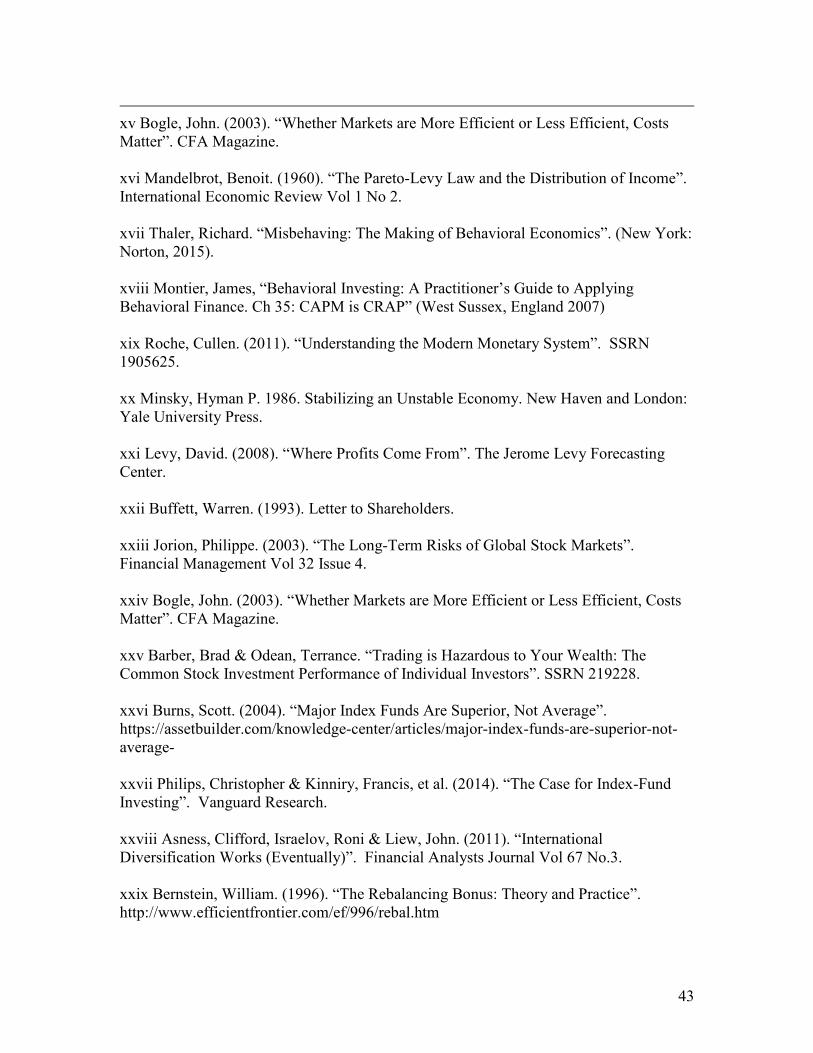
43

xv Bogle, John. (2003). “Whether Markets are More Efficient or Less Efficient, Costs Matter”. CFA Magazine. xvi Mandelbrot, Benoit. (1960). “The Pareto-Levy Law and the Distribution of Income”. International Economic Review Vol 1 No 2. xvii Thaler, Richard. “Misbehaving: The Making of Behavioral Economics”. (New York: Norton, 2015). xviii Montier, James, “Behavioral Investing: A Practitioner’s Guide to Applying Behavioral Finance. Ch 35: CAPM is CRAP” (West Sussex, England 2007) xix Roche, Cullen. (2011). “Understanding the Modern Monetary System”. SSRN 1905625. xx Minsky, Hyman P. 1986. Stabilizing an Unstable Economy. New Haven and London: Yale University Press. xxi Levy, David. (2008). “Where Profits Come From”. The Jerome Levy Forecasting Center. xxii Buffett, Warren. (1993). Letter to Shareholders. xxiii Jorion, Philippe. (2003). “The Long-Term Risks of Global Stock Markets”. Financial Management Vol 32 Issue 4. xxiv Bogle, John. (2003). “Whether Markets are More Efficient or Less Efficient, Costs Matter”. CFA Magazine. xxv Barber, Brad & Odean, Terrance. “Trading is Hazardous to Your Wealth: The Common Stock Investment Performance of Individual Investors”. SSRN 219228. xxvi Burns, Scott. (2004). “Major Index Funds Are Superior, Not Average”. https://assetbuilder.com/knowledge-center/articles/major-index-funds-are-superior-not-average- xxvii Philips, Christopher & Kinniry, Francis, et al. (2014). “The Case for Index-Fund Investing”. Vanguard Research. xxviii Asness, Clifford, Israelov, Roni & Liew, John. (2011). “International Diversification Works (Eventually)”. Financial Analysts Journal Vol 67 No.3. xxix Bernstein, William. (1996). “The Rebalancing Bonus: Theory and Practice”. http://www.efficientfrontier.com/ef/996/rebal.htm

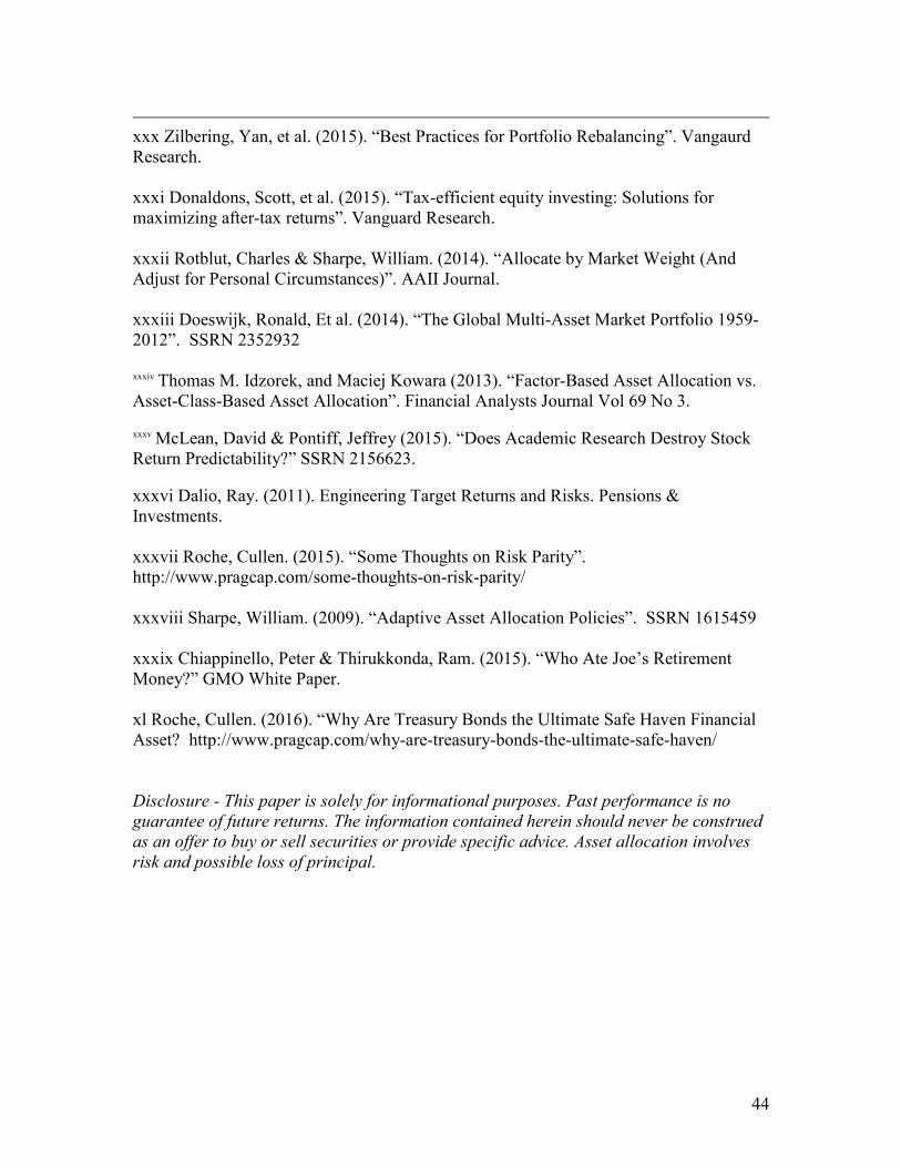
44

xxx Zilbering, Yan, et al. (2015). “Best Practices for Portfolio Rebalancing”. Vangaurd Research. xxxi Donaldons, Scott, et al. (2015). “Tax-efficient equity investing: Solutions for maximizing after-tax returns”. Vanguard Research. xxxii Rotblut, Charles & Sharpe, William. (2014). “Allocate by Market Weight (And Adjust for Personal Circumstances)”. AAII Journal. xxxiii Doeswijk, Ronald, Et al. (2014). “The Global Multi-Asset Market Portfolio 1959-2012”. SSRN 2352932 xxxiv Thomas M. Idzorek, and Maciej Kowara (2013). “Factor-Based Asset Allocation vs. Asset-Class-Based Asset Allocation”. Financial Analysts Journal Vol 69 No 3. xxxv McLean, David & Pontiff, Jeffrey (2015). “Does Academic Research Destroy Stock Return Predictability?” SSRN 2156623.

xxxvi Dalio, Ray. (2011). Engineering Target Returns and Risks. Pensions & Investments. xxxvii Roche, Cullen. (2015). “Some Thoughts on Risk Parity”. http://www.pragcap.com/some-thoughts-on-risk-parity/ xxxviii Sharpe, William. (2009). “Adaptive Asset Allocation Policies”. SSRN 1615459 xxxix Chiappinello, Peter & Thirukkonda, Ram. (2015). “Who Ate Joe’s Retirement Money?” GMO White Paper. xl Roche, Cullen. (2016). “Why Are Treasury Bonds the Ultimate Safe Haven Financial Asset? http://www.pragcap.com/why-are-treasury-bonds-the-ultimate-safe-haven/ Disclosure - This paper is solely for informational purposes. Past performance is no

guarantee of future returns. The information contained herein should never be construed

as an offer to buy or sell securities or provide specific advice. Asset allocation involves

risk and possible loss of principal.