Unbundling Cable Television: An Empirical Investigation

Dmitri Byzalovy

Temple University

July 2010

Abstract

I develop an empirical model of demand for large bundles, and use it to analyze bundling

of channels in cable television. Concerns over cable companiesbundling practices and rapid

price increases have led to an active policy debate about government-mandated unbundling, i.e.,

requiring cable companies to o¤er subscriptions to themed tiersor individual channels on a

la carte basis. I focus on the likely short-run e¤ects of unbundling policies for consumers, cable

networks and cable operators.

I model consumers choice of cable and satellite packages (bundles of channels) and their

subsequent viewing choices for individual channels in the bundle. The main identifying assump-

tion is that consumerswillingness to pay for a bundle of channels is driven by the utility they

get from viewing those channels. This allows me to identify consumersWTPs for individual

channels, even though they are always sold in large bundles, and to predict their subscriptions

and viewing choices in unbundling counterfactuals. I estimate the model using individual-level

data on cable and satellite subscriptions and viewing choices for 64 main cable channels.

I use the estimates to simulate the themed tiersunbundling scenario, which involves break-

ing up the bundle into 7 mini-tiers by channel genre. I nd that consumers do not gain much

from unbundling. The best-case increase in consumer surplus is estimated at just 35 cents per

household per month. At the same time, cable networks are likely to lose a lot of subscribers,

which will signicantly reduce their license-fee revenues. The loss of subscribers is likely to force

the networks to sharply increase the wholesale license fees they charge per subscriber, in which

case unbundling would hurt consumers.

I am especially grateful to Bharat Anand, Julie Mortimer and Ariel Pakes for their guidance and suggestions.I would also like to thank Susan Athey, Ulrich Doraszelski, Anita Elberse, Gregory Lewis, Harikesh Nair, SridharNarayanan and Minjae Song, and seminar participants at Harvard University, IIOC, Summer Institute in Competi-tive Strategy, Stanford GSB, Temple University, University of Rochester and Yale SOM for helpful discussions andcomments. All remaining errors are mine.

yDepartment of Accounting, Fox School of Business, Philadelphia, PA 19122, dbyzalov@temple.edu

1

1. Introduction

I develop an empirical model of demand for large bundles, and use it to analyze the e¤ects of

bundling in cable television. A typical cable package is a bundle containing dozens of channels,

and most consumers watch only a small fraction of the channels they are paying for. For example,

in 1995, an average cable household was paying for a bundle of 41 channels, but watching only 10

of them (24%).1 By 2005, an average cable household was paying for 96 channels, and watching

just 15 of them (16%). The price of a typical cable subscription increased by 93% over the same

period, far outpacing ination (28%).2

Concerns over rapid price increases and cable companiesbundling practices have led to an

active policy debate regarding government-mandated unbundling, i.e., requiring cable companies

to break up their main retail packages, and to allow consumers to pick individual channels or

small themed tiers on a la carte basis.3 Supporters of unbundling policies (various consumer

organizations, and, until recently, the FCC4) argue that it would signicantly benet consumers,

by reducing their cable bills and giving them more choice. On the other hand, opponents of

unbundling policies (most of the cable companies and programmers) argue that it would increase

cable prices and destroy the economic foundations of the cable networks, reducing the quality and

diversity of programming in the long run.5 More than 80% of US households subscribe to cable

or satellite, and an average cable household spends more than 8 hours a day watching television

(Nielsen [2006]) and more than $600 a year paying for it (FCC [2005a]), so a lot is at stake in this

policy debate. However, empirical evidence is scarce (in fact, the only empirical analysis of cable

unbundling I am aware of is the parallel papers by Crawford and Yurukoglu [2008, 2009], discussed

later).

In the empirical analysis, I address two main questions. First, what are the likely e¤ects of

unbundling policies for consumers? The answer to this question is key to the debate, since the push

for unbundling is based on the argument that it will substantially benet consumers. Second, what

are the likely e¤ects for the industry? Specically, how will it a¤ect prices, subscriptions, ratings

and prots for cable operators and cable networks? Importantly, I focus on the short-run e¤ects,

1Souce: Nielsen Research, www.nielsenmedia.com.2FCC (2006).3For example, in response to requests from members of Congress, the Federal Communications Commission (FCC)

and the Government Accountability O¢ ce (GAO) have published three reports (FCC [2004, 2006], GAO [2003])analyzing the e¤ects of a switch to full a la carte or themed tiers, and the then FCC chairman Kevin Martinargued for unbundling in numerous congressional hearings (e.g., November 2005, April 2007, April 2008). Legislationfor cable unbundling was introduced in Congress on several occasions (by Senator John McCain in 2006, and byRepresentatives Dan Lipinski and Je¤ Fortenberry in 2008), however it did not get much traction in the committees.Notice that there is also a separate (but closely-related) debate about wholesale unbundlingin the upstream marketfor cable programming.

4The FCC actively pushed for unbundling under former Chairman Kevin Martin (2005-2009), but made it a lowerpriority under current FCC Chairman Julius Genachowski (since 2009).

5Reports by FCC (2006) and Booz, Allen, Hamilton (2004) are representative of the two sidesmain arguments.Although the two reports reach very di¤erent conclusions, both acknowledge lack of any serious empirical evidenceon the key issues in this debate (e.g., Booz, Allen, Hamilton [2004] page 19, FCC [2006] page 39).

2

i.e., I hold the set of available networks and the quality of their programming xed. One major

concern about unbundling is that it can sharply reduce cable networkssubscriber base and ratings

(their two main sources of revenue), which in the long run can destroy many niche networks and

force others to sharply cut their investment in programming. Thus, the short-run outcomes for the

networks can have important long-run welfare e¤ects for all market participants.

Unbundling at the retail level is likely to dramatically alter the equilibrium in the wholesale

market for cable programming (see section 2.2 for details). While full analysis would require a

credible empirical model of the wholesale market, which is likely to be prohibitively complex,6 I

use a simpler approach. Specically, rst I estimate a detailed model of consumersdemand for

cable bundles and their viewing choices, which allows me to predict their unbundled subscriptions

and viewing choices (for a given vector of retail prices) in counterfactuals. In counterfactuals, I

compute cable operatorsoptimal choice of unbundled retail prices, treating the structure of their

programming costs (the license fees they pay to the networks) as exogenously given. I explore

several alternative scenarios for the programming costs, which allows me to bound the range of

likely short-run e¤ects of unbundling.

The empirical model allows me to address an additional question. Specically, how important

are the discriminatory e¤ects of bundling in the data? The price-discrimination theory of bundling

(e.g., Stigler [1963], Adams and Yellen [1976], Schmalensee [1984], McAfee et al [1989]) is one of

the main explanations for the widespread use of bundling, and cable television is often cited as

a natural example to illustrate this theory (e.g., Salinger [1995], Bakos and Brynjolfsson [1999]).

However, empirical evidence is scarce. In fact, the only empirical study I am aware of that focuses

on the discriminatory e¤ects of bundling is Crawford (2008). He presents reduced-form evidence

for cable television that o¤ers some support for the price-discrimination theory. In addition, several

empirical papers analyze other aspects of bundling. In particular, Chu, Leslie and Sorensen (2006)

analyze simple alternatives to mixed bundling for season tickets, Crawford and Yurukoglu (2008,

2009) analyze the welfare e¤ects of unbundling policies in cable television, and Ho, Ho and Mortimer

(2008) analyze the e¤ects of full-line forcing contracts in the video rental industry.

Bundling is common in many markets (for example, software suites, season tickets, triple-

play bundles), and possible anticompetitive e¤ects of bundling have drawn a lot of attention from

researchers and policymakers.7 Theoretical literature identies several e¤ects of bundling.

First, as mentioned above, bundling may have discriminatory e¤ects, facilitating surplus

extraction by the rm. The sign and magnitude of this e¤ect depends on the covariance structure

of preferences for the bundled goods, since the rm can extract a greater fraction of the total surplus

6Specically, it would have to realistically capture bargaining between programmers such as Disney and cableoperators such as Comcast, in which both sides have substantial market power and negotiate complex multi-yearmulti-channel deals. Crawford and Yurukoglu (2009) explicitly model the bargaining in this market, but to do that,they have to introduce a number of highly restrictive assumptions for tractability (for example, they have to ignorethe multi-channel nature of actual bargaining in this market).

7For example, the rst theoretical exposition of discriminatory e¤ects of bundling, Stigler (1963), was inspired byantitrust cases focusing on block-booking of movies. Recent high-prole examples include the Microsoft case and theantitrust review of the proposed merger between GE and Honeywell.

3

if consumersbundle valuations (the total for all the goods in the bundle) are less heterogeneous.

Bakos and Brynjolfsson (1999) show that this e¤ect is likely to be particularly strong for large

bundles, such as cable packages. In general, this e¤ect has ambiguous implications for consumer

surplus, prots and total welfare. The signs and magnitudes of these welfare implications depend

on the covariance structure of preferences and the marginal costs of the bundled goods.

Second, bundling may have entry-deterrence or leverage e¤ects (e.g., Whinston [1990], Nale-

bu¤ [2000, 2004], Bakos and Brynjolfsson [2000]). There are widespread concerns about entry-

deterrence and leverage e¤ects in the upstream market for cable programming.8 However, at the

retail level (the main focus of my analysis), entry-deterrence e¤ects do not appear to be relevant.9

Likewise, the leverage e¤ects of bundling are unlikely to be important at the retail level, for two

reasons. First, most cable programming is available to all market participants, so there is not much

exclusive programming that could be leveraged via bundling (the only exception is certain types

of on-demand and local sports programming discussed in section 2.2). Second, for cable television,

the leverage mechanism (which works by forcing consumers who want the exclusive good to buy

the other goods from the same rm) does not require bundling. Notice that, with or without

bundling, consumers are unlikely to combine subscriptions from multiple retail providers (for ex-

ample, Comcast and DirecTV), because doing so would double their equipment charges and other

fees. Thus, while exclusive access to programming might give a cable operator an advantage against

its competitors (which my demand model allows to capture), the role of bundling in leveraging this

advantage is minor.

Third, bundling may provide e¢ ciency benets such as economies of scale or scope, or simpler,

more convenient choices for consumers (see Nalebu¤ [2003] for a review of such benets). For

cable companies, the main e¢ ciency benets of bundling are lower equipment and customer-service

costs.10 Also, as mentioned earlier, retail unbundling will signicantly a¤ect the wholesale market

for cable programming. For reasons discussed in section 2.2, the wholesale prices (networkslicense

fees per subscriber) are likely to increase a lot after unbundling.

Unbundling can benet consumers in several ways in the short run. If the discriminatory

e¤ects of bundling are strong, unbundling may signicantly reduce cable operatorsability to extract

surplus from consumers, resulting in a transfer of surplus from cable operators to consumers. Also,

depending on how it a¤ects the total costs of cable programming, it may result in a transfer of

surplus from networks to consumers. Besides redistribution of surplus, unbundling may increase

the total surplus, by partially serving consumers who are ine¢ ciently excluded under bundling

(e.g., current non-subscribers who value ESPN at more than its unbundled price). On the other

8For example, Consumers Union outlines possible anticompetitive e¤ects in its FCC ling (Aug 13, 2004), availableat hearusnow.org/cablesatellite/5/.

9 In the past 15 years there was successful entry by DirecTV and Dish, and (so far) successful entry by VerizonFiOS and AT&T U-Verse. Thus, entry barriers created by bundling (if there are any) are not insurmountable.10Unbundling would require much wider deployment of digital set-top boxes, capable of blocking exible combina-

tions of channels. However, cable operators are gradually switching to all-digital networks anyway (e.g., MultichannelNews, June 26, 2008), so this factor is becoming less important. Also, unbundling is likely to increase the numberand length of calls at cable operatorscall centers, driving up their customer-service costs.

4

hand, it may reduce total surplus, by ine¢ ciently excluding some of the current bundle buyers

(e.g., those who value ESPN at above zero but below its unbundled price), and by increasing the

equipment and customer-service costs. The combined e¤ect of these factors is ambiguous, making

it an empirical question.

The main challenge in the empirical analysis is to identify consumersvaluations for individual

channels. In order to predict the outcomes in unbundling counterfactuals and to characterize the

e¤ects of bundling, I need to estimate consumerswillingness to pay for each channel, as well as the

covariance structure of their WTPs across channels, since it is driving the discriminatory e¤ects of

bundling. However, most channels are always sold in large bundles containing dozens of channels, so

I do not observe any unbundled sales for most channels (the only exception is premium channels like

HBO, which are sold on a la carte basis). Thus, while consumersbundle choices reliably identify

their valuations for entire bundles, I need a way to break them down into channel valuations.

My identication strategy is based on combining data on consumers purchases (of entire

bundles) with additional data on their viewing choices (for individual channels). The fundamen-

tal assumption is that consumers subscribe to cable television because they want to watch cable

television. Thus, their valuation of a bundle of channels is driven the utility they expect to get

from viewing those channels. The viewing utilities for individual channels can be identied from

consumersobserved viewing choices. Notice that the viewing data allows me to identify the joint

distribution of consumersvaluations for individual channels despite the fact that these channels are

always sold in large bundles. Next, expected viewing utility for the bundle is the result of explicit

utility maximization over the channels in that bundle. This links bundle utility to channel utilities

in a fully structural, internally-consistent way. Finally, by combining it with data on consumers

bundle choices and prices, I can link viewing utilities to dollars.11

To implement this approach, I develop a structural empirical model in which I jointly model

consumerschoice of a bundle of channels and their viewing choices conditional on that bundle.

Notice that consumers self-select into di¤erent bundles depending on their unobserved viewing

preferences, therefore it is important to model their viewing and bundle choices jointly, in order

to account for this self-selection.12 The viewing part of the model is rooted in a standard random-

utility discrete-choice framework, which allows me to account for substitution among channels.

Since cable bundles contain dozens of channels competing for consumerslimited time, substitution

among them is likely to be important. For example, the contribution of CNN to the value of a

bundle likely depends on whether it also includes Fox News and MSNBC. By linking bundle utility

to channel utilities via explicit utility maximization, I can fully account for such interactions.

11The same approach was used earlier by Ho (2006). She estimates demand for managed care plans, which o¤eraccess to a network of hospitals (among other things). She measures the contribution of each hospital to the valueof the plan for consumers, using data on their hospital choices. Crawford and Yurukoglu (2008, 2009) use the sameapproach.12For example, suppose that those with higher viewing preferences are also more likely to subscribe to cable. If

this self-selection is ignored in estimation, the model would overpredict the utility of cable television for currentnon-subscribers. Consequently, it would overestimate the welfare gains from unbundling for current non-subscribers(notice that some of them would buy the channels they value after unbundling).

5

I estimate the model using individual-level data from Simmons Research, which contains

consumersviewing choices for 64 main cable channels and their subscriptions to cable and satellite,

combined with several additional sources of data. Compared to more widely-available market-

level data, individual-level data provides several important advantages. First, since I directly

observe subscriptions and viewing choices for the same household, I can account for consumers

self-selection into di¤erent bundles driven by their unobserved viewing preferences. Second, I

directly observe choices of multiple channels for the same individual, and I directly observe viewing

choices by multiple individuals within the same household. This allows me to accurately identify

the covariance structure of preferences (the key driver of the discriminatory e¤ects of bundling),

both across channels and across individuals within the household. Thus, the main advantage of

individual-level data is that it allows one to directly observe the empirical joint distribution of

various outcomes. In contrast, even with very detailed market-level data, one only observes the

marginal distributions, separately for each outcome. As a result, the identication of self-selection

and covariances in market-level data has to rely heavily on functional form assumptions.

A closely-related, parallel paper by Crawford and Yurukoglu (2008) focuses on the same main

question and uses a similar identication strategy. The main di¤erences between our papers are

driven by the di¤erences in the data. Specically, I use individual-level data, while Crawford and

Yurukoglu use market-level data (local ratings and market shares for a large number of markets). As

discussed above, the main advantage of individual-level data it that it allows one to get much more

accurate estimates of the covariance structure of channel preferences, and to properly control for

self-selection, both of which are crucial for evaluating the magnitude of discriminatory e¤ects.13 In a

follow-up paper, Crawford and Yurukoglu (2009) expand the analysis by endogenizing the wholesale

prices of cable programming in the upstream market. They explicitly model the bargaining between

cable networks and cable operators in the upstream market, which allows them to predict the change

in upstream prices (networkslicense fees per subscriber) after unbundling. The retail part of the

model, and the related data limitations, are similar to those in Crawford and Yurukoglu (2008).

I use the estimates to simulate the (short-run) e¤ects of unbundling policies. My main

unbundling counterfactual is themed tiers, in which the cable bundle is broken up into seven

mini-tiers based on channel genre.14 I compute the outcomes for retail prices, subscriptions and

viewership for several alternative scenarios on how cable operatorsprogramming costs change after

unbundling. Notice that unlike Crawford and Yurukoglu (2009), I do not attempt to endogenize the

upstream prices. Instead, I consider several exogenously-given scenarios for how the upstream prices

will change after unbundling. The main reason is that a bargaining model that can realistically

capture the key institutional details of the upstream market (long-term contracts that cover multiple

channels15) would be prohibitively complex. Furthermore, based on my estimates, I nd that there

13Another potentially important di¤erence is in how we model the substitution patterns among channels. I capturethem in a fully structural way, while Crawford and Yurukoglu rely on approximations.14This is one of the main unbundling scenarios in FCC (2006). Another widely-discussed option is unbundling to

the level of individual channels. For reasons discussed in section 7, I use the mini-tiers as my primary scenario.15Notice that the multi-channel nature of these arrangements is important in practice, and leads to frequent

6

is simply no need to add an extra layer of assumptions required to endogenize the upstream prices,

since my predictions for simpler scenarios yield su¢ ciently informative bounds on the welfare e¤ects

of unbundling.

I nd that consumers do not gain much from unbundling. Even if the cable networks do

not increase their wholesale license fees per subscriber after unbundling (the best-case scenario

for consumers), the average gain in consumer surplus is estimated at just 35 cents per household

per month.16 Cable networks license-fee revenues drop substantially in this case, because cable

subscribers are no longer forced to subscribe to the networks they do not value. If the networks

increase their license fees per subscriber to try to o¤set this loss of revenue, consumer end up being

worse o¤ than they were under bundling. Thus, my results do not support the main justication

for unbundling (gains to consumers), but they do support the main concern about unbundling

(signicant loss of revenue for the networks).

Surprisingly, I nd that there are no strong discriminatory e¤ects of bundling. In other

words, bundling does not facilitate surplus extraction from consumers by cable operators, relative

to unbundled sales. The reason is that consumers bundle valuations are quite heterogeneous,

despite the size of a typical cable bundle, and this heterogeneity constrains cable operators ability

to extract surplus via bundling. The lack of discriminatory e¤ects explains why consumers do not

gain much from unbundling: cable operators can extract surplus from them with equal e¤ectiveness

through unbundled sales.

In the next section, I discuss the relevant industry background. In section 3, I present a

simplied version of the model, to illustrate the logic of my approach. Sections 4-7 present the

data, empirical specication, estimation and empirical results. Section 8 concludes.

2. Industry Background

I focus on the subscription television industry in years 2003-2004 (before the entry by Verizon FiOS

and AT&T U-verse, before triple-play bundles, and before widespread adoption of DVRs). I discuss

the retail level of the industry rst, and after that the upstream interactions between cable and

satellite operators and other players in the market.

2.1. Retail Level

There are three ways to receive television programming: local antenna, cable and satellite. In 2004,

16% of TV households in the US used local antenna, 65% subscribed to cable and 19% to satellite

(FCC [2005a]). Local antenna reception is free, but it only provides access to the local broadcast

disputes between cable operators and programmers. For example, a well-publicised dispute between Echostar (Dish)and Viacom erupted after Viacom tried to force Echostar to carry a large number of Viacoms less popular channelsas a condition for getting access to its popular channels (Multichannel News, March 8, 2004).16The welfare e¤ects of unbundling are heterogeneous across consumers, with the worst outcomes for larger, poorer

households.

7

channels (ABC, CBS, NBC, FOX, etc.), and the quality of reception is often low. Unlike broadcast

channels, cable channels (such as CNN or ESPN) are only available on subscription basis, on cable

and satellite.

Most areas are served by one cable operator.17 Cable operators o¤er several packages (tiers)

of TV channels, typically basic, expanded-basic and digital-basic packages.18 The general structure

of cable packages is similar everywhere, but there is a lot of variation in prices and channel lineups

across locations, illustrated in section 4.2.

Basic package contains the local broadcast channels, and cable operators usually add a few

cable channels. Its price is usually regulated by the local franchise authorities, while other packages

and services are not subject to regulation. Expanded-basic package contains the main cable channels

(CNN, ESPN, MTV, TNT, etc.), and it is usually the largest, most expensive package. Digital-basic

package contains additional channels. As of January 2004, the average prices were $18.08 a month

for basic cable, $27.24 for expanded-basic (on top of the basic price), with 44.6 cable channels on

average, and $16.05 for digital-basic (on top of the other two packages), with 31.6 extra channels

on average (FCC [2005b]). All cable subscribers have to get the basic package, and 88% of them

also subscribe to expanded basic, and 35% to digital basic (FCC [2005b]). In addition, consumers

can subscribe to premium channels such as HBO or Cinemax. Premium channels are o¤ered on a

la carte basis, at an average price of about $10-$12 per month.19

The main alternative to cable is satellite, o¤ered by DirecTV and Dish Network.20 Satellite

television is available everywhere in the US, however its availability varies within each area (and

even within the same building) due to physical reasons.21 Satellite operators o¤er several base

packages, roughly equivalent to digital cable in terms of channel lineup, plus premium channels

and several special-interest mini-tiers such as foreign-language programming or additional sports

channels. Unlike cable, there is no regional variation in prices and channel lineups for satellite.

Besides the subscription fees, another potentially important cost for satellite subscribers is the cost

of installation and equipment (satellite dish and receiver). However, in 2003-2004 satellite operators

were o¤ering free installation and equipment in exchange for a one-year commitment (FCC [2005a]).

2.2. Industry Structure and Contracts

17The only exception is several overbuildcommunities with two competing cable operators, a dominant incumbentand a relatively recent entrant (overbuilder). However, such communities account for just 3.1% of cable subscribersin the US, and overbuilders account for less than a fth of those 3.1% (FCC [2005b]).18Entry-level familypackages were introduced later. Some cable systems also o¤er digital mini-tiers of additional

foreign-language channels, movie channels or sports channels.19Consumers have to get basic cable (but not higher tiers) in order to be able to subscribe to premium channels.

Many cable systems also o¤er a multiplexed version of the premium channels (e.g., multiplexed HBO is a mini-package containing HBO, HBO2, HBO Family and HBO Signature).20The market share of other satellite providers (Voom, older large-dish systems) is negligible. Verizon FiOS and

AT&T U-verse entered the market later.21Satellite reception requires an unobstructed direct line of sight from the satellite to the dish antenna on the

customers house. Thus, satellite availability depends on the latitude and terrain, and within the same area, it islower in apartment buildings and for renters (see Goolsbee and Petrin [2004] for details).

8

The main players in the upstream market are the cable networks and cable and satellite operators.

Cable networks create their own programming or purchase it from studios, and deliver it to cable

and satellite operators via a satellite uplink. Cable and satellite operators bundle the networks into

retail packages and distribute them to consumers.

Cable networks have two main sources of revenue, advertising and license fees from cable and

satellite operators (on average, each is about half of the total). Most of the advertising time is sold

by the networks, while cable operators get about 2 minutes per hour for local advertising.

Carriage agreements between the networks and cable operators are negotiated on long-term

basis (up to 10 years). The contracts specify the license fee per subscriber, and often also the tier

on which the network will be carried. Major sports networks charge the highest fees, for example

ESPN charges cable operators $2.28 per subscriber per month on average, and FOX Sports $1.34

per subscriber (2004 data from SNL Kagan [2007]).22 The most expensive non-sports channels

are TNT ($0.82), Disney Channel ($0.76), USA ($0.44) and CNN ($0.43), while the fees for other

major channels range between $0.10-$0.34 per subscriber per month, and most fringe channels

are under 10 cents per subscriber.

Most of the cable networks are owned by one of the large media companies,23 and the carriage

agreements are typically negotiated as a package deal for multiple networks owned by the same

company. Thus, even though the license fees in the data (SNL Kagan [2007]) are quoted separately

for each network, actual contracts are usually for wholesale bundles of networks. Furthermore, the

wholesale bundling requirements in these contracts appear to be practically important.24

Unbundling at the retail level is likely to dramatically alter the wholesale market for cable

programming. Several factors may lead to sharp increases in networkslicense fees per subscriber.

First, subscriptions for most channels will probably drop a lot after unbundling, since cable sub-

scribers will no longer be forced to get the channels that they do not value. Second, networks might

have to increase their marketing expenditures a lot, in order to attract and retain subscribers.25

The e¤ect of unbundling on networksratings and advertising revenues is ambiguous. On the one

hand, it will likely eliminate most of the occasional viewers (those who value a given channel some-

what, but not enough to pay the unbundled price for it). On the other hand, some channels may

gain viewers, if unbundling reduces the number of other channels consumers subscribe to, or if it

attracts additional subscribers to cable. The change in the audience composition may also increase

22These are average license fees for each channel. The license fees vary across cable operators depending on theirbargaining power and specic terms of the contracts (which are highly proprietary).23For example, among the 64 cable networks in my viewing data, 43 (67%) are owned by the 5 largest media

companies (Disney, NBC Universal, News Corporation, Time Warner and Viacom). The same companies own the 4main broadcast networks (ABC, CBS, NBC, FOX).24For example, there was a well-publicised dispute between Echostar (Dish Networks) and Viacom in 2004 that

centered on wholesale bundling of channels by Viacom (e.g., Multichannel News, March 8, 2004). The AmericanCable Association also argues that wholesale bundling forces them to carry a lot of costly undesired programming inorder to get access to the desired programming (americancable.org).25For example, the marketing expenditures for premium networks (sold a la carte) are between 15-25% of sales, vs

2-6% for the expanded-basic networks sold as a bundle (Booz, Allen, Hamilton [2004]).

9

or reduce the advertising rates per rating point.26 Several additional factors may help o¤set the

increases in the license fees. Specically, retail unbundling will change the nature of wholesale price

competition among the networks, by eliminating wholesale bundling of channels by large media

companies, and by forcing the networks to directly compete for subscribers (in addition to existing

competition for viewers and advertisers).27 These changes may result in a more competitive whole-

sale market for cable programming. While the total e¤ect of retail unbundling on the license fees is

highly uncertain, both opponents and supporters of unbundling (e.g., Booz, Allen, Hamilton [2004]

and FCC [2006]) agree that the fees per subscriber are likely to go up (even though they disagree

on how much they will go up). In addition to the short-run e¤ects discussed above, unbundling

is likely to have a major long-run e¤ect on networksentry, exit and investment in programming,

with important welfare implications in the long run.28

The main source of revenue for cable operators is monthly subscription fees for television

services ($50.63 per subscriber on average, which accounts for 67% of their total revenue). In

addition, they get revenue from their share of advertising time ($4.60 per subscriber on average,

6% of total revenue) and other services, such as phone, internet, video-on-demand, installation

and equipment (27% of the total; all revenue numbers are national averages for 2004 from FCC

[2005a]).29 License fees to the networks are by far the largest component of cable operatorsmarginal

costs, totaling $15.95/month per subscriber on average (FCC [2005a]). From conversations with

industry executives, they treat most other expenditures (including customer-service costs) as xed

costs.

Several large cable operators are vertically integrated with cable networks. The largest

vertically-integrated rm in my sample period is Time Warner (the owner of Time Warner Cable),

which fully owns CNN, Cinemax, HBO, TBS, TNT, and 24 other national cable channels.30 Other

large cable operators own quite a lot of channels, but most of them are regional or niche channels,

with relatively few major national channels.31 Vertically-integrated cable operators are required

to make their channels available to competitors on reasonable terms, and exclusive contracts are

26For example, if advertisers value the total reach of their advertising (the number of unique viewers reached atleast once), then the exclusion of occasional viewers can reduce the advertising rates per rating point. On the otherhand, if advertisers value the ability to reach a well-dened niche audience, advertising rates can increase.27Under bundling, networks compete to gain carriage on cable systems, or to be placed on a more popular tier by

the cable operator, but they do not directly compete with each other for retail subscriptions.28Opponents and supporters of unbundling o¤er widely divergent long-run projections, ranging from large declines

in quality or complete destruction of many networks (Booz, Allen, Hamilton [2004]) to emergence of a more vibrantand diverse programming market (FCC [2006]).29Triple-play bundles were introduced later, but by 2003-2004 cable companies were o¤ering broadband internet in

most markets, and phone services in relatively few markets.30Time Warner has since separated Time Warner Cable through a spin-o¤, completed in March 2009

(http://ir.timewarnercable.com/separationfaq.cfm).31Other large vertically-integrated operators are Cablevision, Comcast and Cox. They own some of the major

regional sports networks and local news channels, but few of the major national networks. For example, amongthe 64 national cable channels in my viewing data, Cablevision, Comcast and Cox combined have partial ownershipin 13 channels, and these are mostly fringe channels (they account for less than 12% of the total cost of cableprogramming).

10

generally not allowed (FCC [2005a]).32

3. Basic Model Specication

In this section, I present a simplied version of the empirical model, to illustrate the general logic

of my approach. For clarity, I keep it as simple as possible, and defer most of the practical details

to the empirical specication in section 5.

The model is a two-stage model of demand for bundles of channels and TV-viewing. In

the rst stage, I model households decision to subscribe to a bundle of channels. Notice that

a bundle refers to the combination of all packages and premium channels purchased by the

household, for example basic+expanded-basic+HBO (in unbundling counterfactuals, each

possible combination of channels or mini-tiers is treated as a separate bundle). In the second stage,

I model the viewing choices for each individual within the household, conditional on the bundle

they subscribe to.

The key assumption is that consumers bundle subscriptions in stage 1 are driven by the

utility they expect to get from watching the channels in the bundle in stage 2. Thus, stage 2

identies the utility they get from viewing each channel, while stage 1 links bundle choices to

viewing utilities and prices. The time frame of the model is dictated by the structure of my data (a

cross-section of viewing times for each channel over the past week for each individual, with multiple

individuals observed for each household).

It is more convenient to present the model backwards: rst the viewing choices conditional

on the bundle, then the bundle subscription choice.

3.1. Stage 2: TV-viewing Conditional on the bundle

Household h subscribes to bundle Sh; where Sh lists the channels in the bundle. Household members

i = 1:::Kh have observed characteristics Xh;i and unobserved (to the researcher) characteristics

wh;i. There are T periods per week.33 In each period t, individual i can choose to watch one of the

channels in the bundle (j 2 Sh) or the outside alternative j = 0.Her utility from watching channel j 2 Sh in period t follows a standard random-coe¢ cients

specication

Uh;i;j;t = j + Zjh;i + "h;i;j;t

where j is the vertical characteristic of channel j, Zj are its horizontal characteristics, h;i are

individual is preferences, and "h;i;j;t are i.i.d. logit (type-I extreme value) shocks. The preferences

32There are several exceptions. Specically, DirecTV has exclusive rights to NFL Sunday Ticket, and cable operatorshave exclusive rights to regional sports networks in some markets (FCC [2005a]). These exclusive deals exploitloopholes in the regulation.33For simplicity, I treat all time periods the same. With more detailed data, the model can be extended to

accommodate di¤erences across shows or day parts (e.g., daytime and primetime).

11

are specied as

h;i = Xh;i + wh;i

The unobserved component of preferences is specied as wh;i = ewh + ewh;i; where ewh repre-sents unobserved preferences common to all individuals within the household, and ewh;i repre-sents the individual-specic part of unobserved preferences. I specify them as ewh;i s N(0;) andewh s N(0; ); where determines the correlation in unobserved preferences across household

members.34 Matrices ; and scalar are free parameters in estimation.

The utility for the outside alternative j = 0 is normalized to Uh;i;0;t = 0+"h;i;0;t, where "h;i;0;tis an i.i.d. logit shock.

Notice that my actual viewing data is cross-sectional: for each individual, I observe a 64 1vector of time spent watching each of the 64 main cable channels over the past week. Nevertheless,

I chose to model the viewing choices in terms of a discrete-choice panel model (as opposed to a

hazard or duration model that would directly match the structure of my data), for the following

reasons. First, the underlying viewing behavior that actually generates my weekly viewing-time

data is most naturally described in terms of discrete choices over short intervals of time. Second,

by formulating viewing choices in terms of a discrete-choice panel model, I am able to capture

substitution among channels in a clean fully-structural way. Third, it allows me to link bundle

utility to channel utilities in a transparent internally-consistent fashion.35 Notice that I would not

be able to do the same in a duration model. In estimation, I aggregate predicted viewing choices

for all T periods to obtain predicted time spent watching each channel over the past week, and then

I match predicted viewing times to the actual viewing times in the data (see section 6 for details).

Determinants of the discriminatory e¤ects

Discriminatory e¤ects of bundling are driven by the covariance structure of preferences, across

channels for each individual, and across individuals within each household. In turn, these covari-

ances are determined by the parameters ; and ; channel characteristics Zj and the distribution

of demographics Xh;i in the population. For example, if consumers preferences for sports and

family channels are strongly negatively correlated (via either or ), then their valuations for a

bundle of sports and family channels will be less heterogeneous, allowing the rm to extract surplus

more e¤ectively via bundling. This may make bundling more protable than unbundled sales.

Notice that the covariances across di¤erent individuals within the same household are also

important. For example, suppose that a typical household consists of two individuals, one of which

likes sports channels but not family channels, and the other has reverse preferences. In this case,

even though the valuations for sports or family channels are heterogeneous across individuals,

34The covariance matrices of ewh and ewh;i do not have to be proportional to each other. The only reason I imposethis assumption is to reduce the number of parameters.35 In a parallel paper, Crawford and Yurukoglu (2008) use a di¤erent modeling approach, and capture consumers

viewing preferences using a Cobb-Douglas utility function dened over viewing times for di¤erent channels. However,the resulting empirical model is intractable, which forces them to rely on reduced-form approximations to proxy forsubstitution among channels.

12

they are much less heterogeneous across households. As a result, the rm can extract surplus

e¤ectively using unbundled sales, and the heterogeneity-reduction advantage of bundling becomes

less important.

Since cable subscription is a household-level decision, I could simplify the model and estima-

tion by directly modeling household-level viewing preferences, after aggregating the viewing data

from individual to household level. However, by explicitly modeling the viewing choices for each

individual within the household, I can capture the covariance structure of channel valuations (for

entire households) much more accurately. For example, suppose that the main determinants of

viewing preferences (at the individual level) are gender and age. Then, the covariance structure of

household-level channel valuations is likely to be quite di¤erent for di¤erent household types (e.g.,

a married couple of similar ages vs a married couple of dissimilar ages vs a single individual). By

modeling viewing choices at the individual level, I can accurately capture the covariance patterns

for di¤erent household types in a simple and transparent fashion. On the other hand, if one were

to model viewing choices directly at the household level, it would require a much less transparent

reduced-form specication, to account for every possible combination of household members.

Expected viewing utility for bundle ShIn each period, after observing the shocks "h;i;j;t, the individual chooses the alternative that

maximizes her utility among the channels in the bundle (j 2 Sh) and the outside alternative (j = 0).Thus, her realized ex-post viewing utility in period t is equal to

maxfUh;i;j;tgj2fSh;0g

Before the draws of the shocks "h;i;j;t for period t have been realized, her expected viewing utility

for period t is

EU(ShjXh;i; wh;i) EmaxfUh;i;j;tgj2fSh;0g

where the expectation is over the draws of the "h;i;j;t-s. This implicitly assumes that consumers

have perfect information about channel characteristics j ; Zj for all the channels in the bundle.36

Notice that the unobserved preferences wh;i are systematic and known to the consumer, so they are

not absorbed in this expectation, and the only source of uncertainty is with respect to the future

draws of the shocks "h;i;j;t:37

36This assumption is standard in discrete-choice models of demand, i.e., most empirical papers assume that con-sumers have perfect information about the main characteristics of all the alternatives in the choice set, even if itcontains hundreds of products (e.g., cars in Berry, Levinsohn and Pakes [1995]).37 I assume that all the unobservables in channel utilities are either systematic (wh;i) or completely idiosyncratic

("h;i;j;t):With more detailed data, the model can be extended to accommodate a more exible covariance structure ofthe shocks, e.g., I could allow for somewhat-persistent shocks in viewing preferences (such shocks would be absorbedin the expectation).

13

For logit shocks, this expected utility has a simple analytical expression (Ben-Akiva [1973])

EU(ShjXh;i; wh;i) = Emaxfj + Zjh;i + "h;i;j;tgj2fSh;0g

=

= ln

0@ Xj2fSh;0g

expj + Zjh;i

1A (3.1)

Notice that the expected viewing utility for the bundle is not additive with respect to channel

utilities. This is a natural implication of the random-utility discrete-choice framework. The reason

is that di¤erent channels are substitutes for each other at any given moment. Thus, when a new

channel j is added to the bundle, its contribution to bundle utility depends on which other channels

are also included in the bundle, reecting the e¤ect of substitution among channels.

Given the estimates of channel utilities, I can compute expected viewing utility for any bundle

of channels (and not just for the bundles I observe in the data). Notice that this expected viewing

utility is well-dened for any combination of available channels, since it is simply E(max) for

several random variables with a known joint distribution. This feature is crucial for the unbundling

counterfactuals, in which I have to evaluate utility for new bundles never observed in the original

data.38

3.2. Stage 1: Bundle Subscription Choice

Household h chooses a bundle from the menu of all available bundles, which includes local an-

tenna and various combinations of packages and premium channels on cable and satellite.39 The

subscription-stage utility from bundle S at price P is specied as

U(S; P jXh; wh) = F (EU1; :::; EUKh) + (Xh; w

Ph )P (3.2)

where EUi EU(SjXh;i; wh;i) is the expected viewing utility from bundle S for household memberi, F (:::) is a function that aggregates household membersviewing utilities,40 Xh (Xh;1; :::; Xh;Kh

)

and wh (wh;1; :::; wh;Kh) are the observed and unobserved characteristics for all household mem-

bers i = 1:::Kh, and (Xh; wPh ) is the price coe¢ cient that varies across households depending on

their observables Xh (e.g., income) and unobservable wPh .

Given the menu of all available bundles, the household chooses the bundle that yields the

highest utility. After integrating out the unobservables, this yields predicted probabilities for all

cable and satellite bundles. Notice that given the estimates of channel utilities, I can compute

38Notice that the new productsintroduced in counterfactuals are new combinations of existing channels, not newchannels.39For example, if the cable operator o¤ers a basic package, an expanded-basic package and HBO, the list of possible

cable bundles is: (1) basic, (2) basic + HBO, (3) basic + expanded-basic, (4) basic + expanded-basic + HBO.40Average, sum, weighted average, etc whichever ts the data the best. Notice that since EUi is the same for all

periods t (due to data limitations), I do not have to explicitly aggregate utility across periods.

14

expected viewing utility, and therefore predicted choice probabilities, for any new bundle (any

combination of available channels). This allows me to predict bundle choices in out-of-sample

unbundling counterfactuals.

The model does not include any bundle-specic idiosyncratic shocks, such as i.i.d. logit

shocks for each bundle and household. This follows the pure characteristics model of Berry and

Pakes (2007). This feature of the model is important for unbundling counterfactuals, since they

involve introduction of a large number of new bundles in consumerschoice set. For example, if

there are 50 channels, under full a la carte consumers would be choosing among 250 cable bundles

(all possible combinations of channels). So, if the model contained an i.i.d. logit shock for each

bundle, the distribution of the maximum of bundle utilities would be unreasonably high, since at

least some of the 250 i.i.d. logit shocks would be extremely high. This would distort the welfare

e¤ects and the predicted market shares in counterfactuals. Berry and Pakes (2007) show that

the pure characteristics model has more reasonable implications in counterfactuals that involve

introducing a large number of new alternatives in the choice set.

Restrictive Assumptions and Possible Extensions

The main restrictive assumption in the model is that it treats all time periods as identical, i.e.,

the systematic part of channel utilities is assumed to be the same for all t-s. I impose this assumption

because my data is not detailed enough to estimate a more exible specication. However, it can

be done with more detailed viewing data, for example viewing by day part for each channel. In this

case, I could estimate the viewing utilities separately for daytime and primetime for each channel,

and allow the e¤ect of viewing utility on bundle choices to vary by day part (for example, a higher

weight on viewing utility during primetime).

Another potentially important factor is that viewers may value an hour of TV-viewing dif-

ferently depending on the type of programming. For example, consumers might value an hour of

ESPN or HBO more than an hour of the Weather Channel, even if they spend the same amount

of time watching both channels. This could denitely be a major concern about my empirical

approach. However, when I compute predicted unbundled subscriptions for HBO and ESPN as a

sanity check, they turn out to be consistent with the available evidence (see section 7 for details),

mitigating this concern.

3.3. Identication

As mentioned above, I observe multiple individuals within each household. For each individual,

I observe demographics Xh;i and the vector of time spent watching each of the 64 main channels

over the past week. For each household, I also observe its subscriptions to cable or satellite. I also

observe the characteristics of cable packages o¤ered in each location.

The viewing utility parameters (j-s; ; ; ) are identied primarily by the viewing choices in

the data. Individual-level data allows me to get reliable estimates of the parameters in channel pref-

erences, because I directly observe choices of multiple channels for each individual and household,

15

and demographics for the same individual or household. Thus, the covariances between viewing

choices and demographics (which pin down ) and the covariances in viewing choices conditional

on demographics (which pin down and ) are identied directly from the data.

The identication of j ; ; and from the viewing choices is generally straightforward,

the only complication is that households self-select into di¤erent bundle subscriptions depending

on their unobserved viewing preferences !h: Thus, the distribution of !h conditional on the chosen

bundle di¤ers between non-subscribers and subscribers, and it also di¤ers across di¤erent levels of

subscriptions on cable and satellite. Nevertheless, for cable and satellite subscribers, the distribution

of !h can be identied directly from the viewing data for the channels they subscribe to.

However, for non-subscribers (local-antenna households, who do not receive any cable chan-

nels), the distribution of !h is not directly identied from the viewing data.41 Besides identication

through functional form, part of the distribution of !h for them is identied through variation in

characteristics of cable packages (prices and channel lineups) across locations. Notice that the

characteristics of cable packages have no e¤ect on consumersviewing preferences, but they a¤ect

the range of unobserved viewing preferences !h for consumers who self-select into each subscrip-

tion, and therefore they a¤ect the distribution of observed viewing choices among subscribers. For

example, suppose that the cable packages o¤ered in location A are more attractive (lower prices or

better channel lineups) than the packages o¤ered in location B. In this case, some of the households

who would have chosen local antenna in location B would subscribe to cable in location A. Thus,

the distributions of !h among cable subscribers would be di¤erent between locations A and B, and

this di¤erence can be identied by comparing the distribution of observed viewing choices (among

cable subscribers) between the two locations. As a result, I can trace out part of the distribution

of !h for non-subscribers.

Notice that I am able to identify the covariance structure of unobserved heterogeneity even

though I only have cross-sectional viewing times data and not a panel. The reason is that my cross-

sectional dependent variables (viewing times) are continuous variables that capture the outcomes

of multiple discrete choices, as opposed to a cross-section of mutually-exclusive binary variables (a

more typical case for cross-sectional discrete-choice data). Since my dependent variables summarize

the outcomes of multiple discrete choices, their covariance structure contains useful information re-

garding the covariances of the underlying discrete choices, which in turn identies the covariance

matrix of the unobserved heterogeneity in preferences. In contrast, a typical cross-section (of

mutually-exclusive binary variables) contains the outcome of only a single discrete choice, and

therefore it contains absolutely no information about the covariance matrix of unobserved hetero-

geneity.

A secondary source of identication for the viewing utility parameters is through variation

in channel lineups across locations and across tiers, and its e¤ect on bundle choices. For example,

if basic-only subscriptions are higher in areas where ESPN is carried on basic tier (as opposed to

41 I do not have viewing data for broadcast channels (available over the air for free), so I cannot identify thedistribution of !h for local-antenna households from their viewing choices for broadcast television.

16

expanded-basic), the model will attribute it to the viewing utility for ESPN.

The parameters in F (EU1; :::; EUKh); i.e., the e¤ect of expected viewing utility on bundle

choices, is identied from several sources. One source is variation in demographics across house-

holds, which a¤ects both their viewing choices and their bundle choices. The co-movement between

bundle choices and viewing choices, driven by variation in demographics, will identify the e¤ect of

viewing utility on bundle choices.

Another important source of identication for the parameters in F (EU1; :::; EUKh) is vari-

ation in cable packages across locations, illustrated in section 4.2. The e¤ect of channel lineups

on subscription choices, combined with the estimates of channel utilities from the viewing data,

will identify the parameters of F (EU1; :::; EUKh): One issue with this source of identication is

that much of the variation in channel lineups is with respect to the niche channels that relatively

few people watch. However, among those who do watch a given niche channel, the viewing time

patterns are comparable to those for the major channels.42 Thus, even though each niche channel

has a relatively small total audience, its impact on subscriptions among this audience is comparable

to the impact of the major channels. Furthermore, di¤erent people like di¤erent niche channels,

so the combined variation in the availability of niche channels is a¤ecting a large proportion of

consumers. Also, the data has meaningful variation even for the most popular channels such as

CNN or ESPN. Although CNN and ESPN are available everywhere, di¤erent cable systems place

them on di¤erent tiers. For example, about 10% of systems carry ESPN on the basic tier, and 90%

on expanded-basic. If consumers value ESPN, the locations that o¤er ESPN on basic tier will have

a higher share of basic-only cable subscribers, at the expense of other cable and satellite packages

and local antenna. Furthermore, some of the major channels exhibit much more variation than

ESPN (e.g., Discovery, Fox Sports and TBS see section 4.2).

There is enough price variation across locations to identify the price sensitivity parameters.

Notice that despite the use of individual-level data, price endogeneity is still a concern, as discussed

in Berry, Levinsohn and Pakes (2004). Although the channel lineup of a cable package (which

I control for) fully summarizes the main characteristics of that package, important unobserved

determinants of demand may include the quality of customer service and marketing e¤ort. Both

likely vary across cable systems, and both are likely correlated with price. This gives rise to price

endogeneity, which can be dealt with using standard methods.43

42For example, in the data, just 4% of consumers watched the Independent Film Channel (IFC) in the past week,vs 28% for Discovery. However, an average IFC viewer spent 2.7 hours watching IFC, while an average Discoveryviewer spend 2.6 hours watching Discovery.43Another related concern is possible endogeneity of channel lineups. For example, cable operators may o¤er a

more attractive channel lineup in markets with higher (or lower) marketing e¤ort. Most empirical literature in IOassumes that all product characteristics except price are exogenous, and the justication is that they are much harderto change than price. Notice that the same is true for channel lineups. Even though channel lineups are easy tochange from the technical standpoint, cable operators are locked in multi-year contacts which usually stipulate aspecic tier for each network. This constrains their ability to change the channel lineups.

17

4. Data

I use data from several sources. Simmons National Consumer Survey (May 2003 May 2004)

provides individual-level data on cable and satellite subscriptions and viewing choices for the 64

main cable channels. The Television and Cable Factbook (2005) provides characteristics of cable

packages for each location. The license fees data is from SNL Kagans Cable Program Investor.

In the empirical analysis, I focus on 4 metropolitan areas: Boston, Los Angeles, New York

and San Francisco.44 All the descriptive statistics in this section refer to these 4 areas.

4.1. Individual-Level Cable Viewing Data (Simmons National Consumer Survey)

The Simmons National Consumer Survey data is based on a self-administered paper survey con-

ducted between May 2003 - May 2004. For each household, it samples all household members above

age 18.

For each household in the sample, I observe household demographics and some information

on their location and their cable and satellite subscriptions. The subscriptions data consists of

binary variables for: (1) analog cable, (2) digital cable, (3) satellite, and (4) premium channels (six

binary variables for subscriptions to HBO, Cinemax, Encore, The Movie Channel, Showtime and

StarZ).

For household location, I observe state and DMA code.45 Notice that each state and DMA

contain multiple cable systems, with substantial variation in cable packages and prices across sys-

tems. Thus, the location variables in the data are not detailed enough to identify the exact menu

of packages and prices facing each household. In the empirical analysis, I solve this problem by

integrating out households unobserved location within the DMA (section 5.3).

For each individual, I observe demographics and cable viewing data. The viewing data

records how much time the individual spent watching each of the 64 main cable channels over the

past 7 days (a 64 1 vector of viewing times for each individual).46 This data covers most of thecable channels typically carried on basic and expanded-basic tiers (the main exception is regional

sports networks like NESN or YES, which are available locally in some markets but not nationally),

and many of the digital tier channels. The viewing data is self-reported by the respondent at the

end of the week. This reduces the accuracy of the data. On the other hand, a useful advantage

of self-reported data (compared to automatically-recorded Nielsen data) is that the respondent is

44 I drop the rest of the data due to very time-consuming data entry (the Factbook data I have is on paper, andeach large metropolitan area contains dozens of cable systems, with a lot of data for each system). Notice that cableoperators set the prices of their packages locally, so I do not need a nationwide sample to be able to do meaningfulcounterfactuals.45A DMA (Designated Market Area) is a broadcast TV market as dened by Nielsen Research. For the largest

DMAs, the DMA boundaries are roughly similar to the corresponding metropolitan area (for example, Boston DMAcovers most of Eastern Massachusetts and parts of Vermont and New Hampshire). I observe DMA codes only for the14 largest DMAs.46This does not include viewing data for broadcast networks (ABC, CBS, NBC, FOX, etc). The dataset contains

some data for broadcast networks, but the variable denitions are quite di¤erent, and cannot be easily combined withthe cable viewing data in estimation.

18

likely to remember and report the occasions when she was actually watching TV (i.e., paying some

attention), as opposed to TV just being on (which would count as viewing in Nielsen data).

One important issue is missing data. First, even though Simmons attempts to sample all

household members above age 18, many households (about 33%) have missing household members

in the data. In addition, about 5% of respondents did not ll out the cable viewing part of the

questionnaire at all, or reported unreasonable numbers (such as watching TV more than 24 hours

a day). In the empirical analysis, I drop households with missing household members, since cable

subscription is a household-level decision.47 In addition, if a respondent did not ll out the TV-

viewing part of the questionnaire or reported unreasonable total viewing time (dened as above 70

hours a week), I treat her viewing choices as unobserved in the TV-viewing part of the model, but

keep the household in the bundle-choice part of the model. If these data problems are independent

of consumersunobserved viewing preferences, this sample selection does not bias the estimates.

Also, I drop households that do not own a TV (about 2% of the original sample). The nal sample

in the empirical analysis is 2314 households, containing 4846 individuals above age 18, 95% of them

with valid viewing data.

Table 1 summarizes subscription choices in the data. Compared to the national data from

FCC (2005a), the proportion of local-antenna households in the 4 DMAs is somewhat higher (23% vs

16%), and the proportion of cable subscribers is somewhat lower (57% vs 65%). This is reasonable,

since the quality of the outside alternative (not watching TV) is likely to be higher in the 4 large

metropolitan areas I focus on.

Table 2 summarizes viewing choices for each channel, among cable and satellite subscribers.

Notice that the di¤erences in viewership across channels reect not only di¤erences in channel

utilities, but also di¤erences in channel availability and tier placement (both are accounted for in

the empirical model). The most popular channels are CNN, Discovery, HBO, TBS and TNT, with

a weekly audience of 24-28% of all cable and satellite subscribers. Interestingly, even though there

are dramatic di¤erences in audience size across channels, from 0.7% for Fuse to 28% for Discovery,

the average viewing time (conditional on watching a given channel) is comparable, e.g., 2.3 hours

a week for Fuse vs 2.6 hours for Discovery. Thus, even though niche channels appeal to much

fewer consumers than major channels, the intensity of preferences (among their target audience) is

comparable.

Table 3 presents the correlations in viewing times across channels, for several major represen-

tative channels. The correlation patterns are quite intuitive, for example the highest correlations

(for the column channel in the table) are between Cartoon Network and Nickelodeon; CNN and

CNN Headlines/Fox News; Discovery and History Channel; ESPN and ESPN2/FOX Sports; MTV

and VH1. When I compute correlations between each pair of channels in the data, most of them

are close to zero (93% are below 0.2, and two thirds are below 0.1), suggesting large potential for

discriminatory e¤ects of bundling.

47Also, I do not have viewing data and detailed demographics for children within the household. I tried addingreduced-form control for children in households bundle choices, but it was insignicant in all cases.

19

There is a lot of cable viewing by non-subscribers. For example, 39% of local-antenna re-

spondents (who do not receive any cable channels at home) report watching some cable channels

over the past week, and on average they watched about 11 hours of cable last week (among those

who report non-zero time). Furthermore, they watch a wide variety of channels.48 In the empirical

model, I explicitly account for cable viewing by non-subscribers.

4.2. Characteristics of Cable Packages (The Television and Cable Factbook)

The Television and Cable Factbook is the standard source of data for the cable industry. It provides

detailed characteristics of cable packages for each cable system49 in the US. For each system I

observe: (1) locations served by the system, (2) channel lineups and prices for each package, and

(3) prices for the premium channels. I use the 2005 edition of the Factbook, which contains data

for 2004.

The Factbook data su¤ers from two main problems. One is missing data for prices.50 Another

is non-updating of data. For example, when I compare the 2004 and 2005 editions of the Factbook,

the data for most of Adelphia, Cablevision and Charter systems is identical for both years, which

suggests that the data for them was not updated in the 2005 edition. So, the data for them is for

2003 or earlier, however it does not appear to be heavily out-of-date (their channel lineups and

prices are quite similar to those for systems with up-to-date data). On the other hand, the data for

all of Comcast, Cox and Time Warner systems (a majority of all cable systems in my sample) was

updated in the 2005 edition, i.e., the data for them is up-to-date for 2004. Despite these issues,

the Television and Cable Factbook is the standard source of data on the cable industry, both for

industry practitioners and for academic research (e.g., Goolsbee and Petrin [2004], Crawford [2008],

Chipty [2001], Crawford and Yurukoglu [2008, 2009]).

In the empirical analysis, I focus on cable systems in four metropolitan areas (DMAs): Boston,

Los Angeles, New York and San Francisco. I drop overbuildsystems and systems with less than

2000 subscribers.51 My nal sample consists of 140 cable systems, which serve about 8 million

cable subscribers (12% of US total). The cable systems range in size from a few thousand to 1.4

million subscribers (Time Warner Cable in Manhattan), with a median system serving around

30,000 subscribers.

48A recent study by Arbitron also nds that 35% of respondents watch TV outside their home each week (mostlyat a friends house, bars and restaurants, or at work), and their viewership is spread over various genres (Media LifeMagazine, Apr 9, 2007).49A cable system is dened as a community or several communities that are o¤ered the same services at the

same prices from the same cable company. Large cable operators often have dozens of di¤erent cable systems withinthe same metropolitan area, with di¤erent prices and channel lineups.50Prices are missing for 7% of basic packages, 11% of expanded-basic packages, and 25% of digital packages in

my sample. In the empirical analysis, I ll in the missing prices using a regression of package prices on packagecharacteristics, separately for each tier.51Overbuilders (recent cable entrants competing with the incumbent) are present in a very small number of

locations (e.g., some parts of Manhattan). I drop them because I do not observe specic neighborhoods in whichthey are active, and their market share is negligible. I drop the systems with less than 2000 subscribers because theirshare of all subscribers is negligible, while the data entry time is the same as for other (much larger) systems.

20

There is a lot of variation in prices and channel lineups across cable systems. Figure 1

illustrates variation in prices and number of channels for the most popular combination of packages,

basic and expanded-basic packages combined. The price ranges from $11.50 to $63.80, and the

number of cable channels ranges from 13 to 71 (this does not include broadcast channels). Some of

this variation is variation across di¤erent cable operators and across di¤erent metropolitan areas,

however there is also substantial variation across cable systems even when I focus on the same cable

company within the same metropolitan area. Possible reasons for such variation are discussed later

in this section.

Variation in Channel Availability

An important source of identication is variation across cable systems with respect to channel

availability and tier placement. Table 2 presents availability and tier placement numbers for each

channel (all the numbers are weighted averages across cable systems, weighted by system size).

Availability of most niche channels varies across cable systems. However, major cable channels

are available essentially everywhere. For them, the main source of variation is with respect to

their placement on a specic tier (basic, expanded-basic or digital-basic). For some of the major

channels, there is a lot of variation with respect to their placement on digital vs analog tiers. For

example, the break-down between digital and analog tiers is 15% vs 81% for the Sci-Fi channel, 8%

vs 87% for FOX Sports, and 11% vs 83% for the Disney Channel.52

However, the most popular channels (e.g., CNN, ESPN, USA) are never placed on the digital

tier. For them, the variation is with respect to their placement on basic vs expanded-basic tier.

For example, the break-down between basic and expanded-basic tiers is 10% vs 90% for ESPN, 5%

vs 95% for CNN, and 7% vs 93% for USA.53 Thus, there is some meaningful variation even for

the most popular channels. Furthermore, the 5-10% of systems that carry CNN or other major

channels on the basic tier do not appear unusual in terms of average demographics. Also, there is

much more variation for some of the major channels, for example, the break-down between basic

and expanded-basic tiers for TBS is 45% vs 53%, and for Discovery it is 24% vs 73%.

What is driving the variation in cable packages?

Several factors can explain the variation across cable systems. First, the price of basic cable is

usually regulated by the local authorities, which may a¤ect the optimal allocation of cable channels

between basic cable and other packages, and the optimal prices of other packages. Second, some

cable channels are vertically integrated with cable operators, which a¤ects their choice of which

channels to carry. Chipty (2001) nds that vertically-integrated cable operators are more likely

to carry the channels they own, and less likely to carry competitors channels. Also, the terms

of carriage agreements with the cable channels (including wholesale bundling and tier placement

requirements) vary across cable operators, depending on their bargaining power and when they last

52The numbers add up to less than 100% because not all systems carry these channels.53This break-down refers only to the systems that o¤er separate basic and expanded-basic packages (a small

percentage of systems merge them into a single basicpackage).

21

renegotiated the contract.54 Third, even for the same cable operator in the same metropolitan area,

di¤erent locations have di¤erent age and quality of cable infrastructure, which a¤ects the optimal

conguration of cable packages.55 Finally, the distribution of demographics di¤ers across locations,

so it is optimal for cable operators to o¤er di¤erent channel lineups and prices in di¤erent locations.

5. Empirical Specication

The empirical specication follows the general structure of the basic model (section 3), with some

modications and additional details to accurately capture the practical details of cable subscriptions

and viewership.

For each individual i = 1:::Kh within household h, I observe demographics Xh;i and a vector

of viewing times (Th;i;1; :::; Th;i;64) for the 64 main cable channels, where Th;i;j denotes the total

time spent watching channel j in the past 7 days. For each household, I also observe its cable or

satellite subscription. For each location, I observe the characteristics of all available cable packages

(the characteristics of satellite packages are the same everywhere in the US).

The model is presented backwards. First, I present the TV-viewing part of the model (stage

2), conditional on households subscription to a specic bundle of channels. Then, I present the

bundle choice part of the model (stage 1).

5.1. TV-viewing Conditional on the Bundle of Channels (Stage 2)

I model the viewing choices for each individual i = 1:::Kh within household h. The household

subscribes to a bundle Sh, where Sh lists the cable channels in the bundle. Notice that Sh only

refers to cable channels, i.e., it does not include broadcast networks.56 For non-subscribers (local-

antenna households), Sh = ?:There are 7 days, 20 half-hour periods each day. In each period t, individual i chooses one

of the cable channels j or the outside alternative (j = 0). The outside alternative includes not

watching TV or watching one of the broadcast networks.

Channel utilities. Individual i within household h has observed demographics Xh;i and un-

observed preferences wh;i. In each period t, her utility from watching channel j 2 Sh is

Uh;i;j;t = fj(j + Zjh;i + h;i;j) + "h;i;j;t (5.1)

54Also, it appears that the carriage agreements for the broadcast networks are often negotiated with their locala¢ liates, separately for each broadcast market, and the terms of these agreements (including the wholesale bundlingrequirements for the cable channels a¢ liated with the broadcast network) vary across markets.55For example, the capacity of Comcasts system in Boston, MA, is 104 standard 6MHz channels, vs 77 channels in

nearby Cambridge, MA. Besides historical factors and cable companiesgradual infrastructure upgrade schedules, theage and quality of physical infrastructure may be inuenced by the local authorities. For example, in franchise renewalnegotiations with Comcast in 2002, Boston mayor imposed specic deadlines and conditions on its infrastructureinvestment in the city (http://www.cityofboston.gov/cable/franchise.asp).56Although there might be some variation in the availability of fringebroadcast networks, the major broadcast

networks (ABC, CBS, NBC, FOX) are available everywhere, and cable operators are required to carry all of them onthe basic tier.

22

where j is the vertical characteristic of channel j, "h;i;j;t is an i.i.d. logit (type-I extreme value)

shock, and the rest of the terms are discussed below.

The term Zjh;i captures the utility from observed (to the researcher) horizontal channel

characteristics Zj : The preferences for Zj are h;i = Xh;i + wh;i; where Xh;i are individual is

observed demographics; and wh;i are her unobserved preferences. To account for possible within-

household correlations, I specify wh;i as wh;i = ewh + ewh;i; where ewh;i s N(0;); ewh s N(0; ):57

Matrices , and scalar are free parameters in estimation. Channel characteristics Zj include

channel genre and target demographics.58

The next term, h;i;j ; represents channel random e¤ects, with a exible covariance structure

across channels. It captures unobserved channel preferences, beyond the patterns captured by

unobserved preferences for the horizontal characteristics Zj . In principle, one could estimate a

exible 6464 covariance matrix of h;i;j for the 64 channels in the data, however that would requireestimating an unreasonably large number of parameters. To reduce the number of parameters, I

use a factor-analytic specication

h;i;j = jwh;i

where j is a length-M vector of free parameters for channel j, and wh;i are the M common

factors. I specify wh;i as wh;i = ewh + ewh;i; where ewh;i s N(0; IM ), ewh s N(0; IM ); and reects

correlations across household members. The j-s capture the covariance structure of unobserved

channel preferences h;i;j . For example, two channels with similar j-s will have strongly positively-

correlated h;i;j-s, while two channels whose j-s are orthogonal to each other will have uncorrelated

h;i;j-s. Factor-analytic specications are common in marketing (e.g., Elrod and Keane [1995]), but

less common in economics (some exceptions are Sargent and Sims [1977] and Stock and Watson

[1999, 2002]). While the main objective in these papers is to identify a small number of meaningful

common factors, my objective is more modest: to nd a parsimonious reduced-form specication

that approximates the covariances across channels reasonably well. In estimation, I choose the

number of factors M high enough to capture the covariances in the data reasonably well, but low

enough to keep the number of parameters manageable.59

The non-linear transformation fj(j+Zjh;i+h;i;j) allows me to t the main patterns in the

data much better than a more standard linear specication. Specically, when I estimated various

57The only reason I restrict the covariance matrices of ewh;i and ewh to be proportional to each other is to reducethe number of parameters in estimation (the data allows to identify more exible specications).58 I classify all channels into 7 mutually-exclusive genres (see table 2 for details). I compute target demographics

for each channel as the average demographics of its national audience (% males, age, % blacks, % college grads and% households with children). To reduce the number of parameters in estimation, Zjh;i for each of the targetdemographicsvariables in Zj only includes interaction with the corresponding respondent demographic (age entersas a squared di¤erence). Also, I control for the di¤erence between DMA rating and national rating for each channel,to proxy for regional di¤erences in preferences.59One way to think about the identication of M and j-s is as follows. First, estimate the model with a exible

64 64 covariance matrix for h;i;j-s. After that, try to approximate with a much smaller number of parameters; increasing the number of dimensions (i.e., the number of free parameters in ) until the t is good enough: Toreduce the number of parameters, I estimate j only for the 32 most popular channels, which account for about 75%of total viewership, and set it to zero for the rest of the channels.

23

linear specications (with normally-distributed unobserved preferences), the model successfully

captured the mean time spent watching each channel, but heavily overpredicted the proportion of

non-zero viewing times (i.e., in the data, say 10% watch channel j for 3 hours, while the model

would predict 30% watching it for 1 hour). In other words, the model would overpredict the

proportion of consumers with moderately low preferences for channel j (occasional viewers), at the

expense of very low and high preferences. The reason is that normal distribution has the highest

density at moderate preferences. In contrast, the patterns in the data are consistent with a certain

fraction of consumers having high preferences for channel j (heavy viewers), a large majority

having very low preferences (non-viewers), and relatively few consumers having moderately low

preferences (occasional viewers). One natural solution could be to use a di¤erent distribution for

unobserved preferences (e.g., lognormal or exponential). However, I have to model covariances

across 64 channels, across di¤erent product characteristics and across di¤erent household members,

and that would be more di¢ cult to do with a di¤erent distribution (for example, while the sum of

two normal distributions is also normal, and its covariance structure is easy to characterize, this is

not the case for the sum of two lognormal or exponential distributions). Therefore, I use a more

transparent approach, in which I rst build up the covariance structure of preferences using normal

distributions, and then transform the resulting distribution of channel utilities j + Zjh;i + h;i;j

using fj(:::): I specify fj(:::) as

fj(u) = u 01

1 + e1(ufj )

where 0; 1 and f1 :::

fJ are free parameters. It nests the linear specication for 0 = 0: If 1 is

large relative to the range of u = j + Zjh;i + h;i;j ; then fj(u) u for u above the threshold

f1 ; but drops to fj(u) u 0 below the threshold. This transformation allows me to match

the proportion of heavy viewers and non-viewers without overpredicting the number of occasional

viewers.

I do not have viewing data for some of the niche channels in the bundle. I specify the viewing

utility for such channels as Uh;i;j;t = other + "h;i;j;t, where "h;i;j;t is an i.i.d. logit shock.

Also, I observe a lot of cable viewing by non-subscribers in the data. This includes both

local-antenna households watching cable channels, and cable subscribers watching channels that

are not included in their subscription. To capture this in estimation, I allow consumers to watch

channels they do not subscribe to (j =2 Sh), but their viewing utility for such channels is lower:

it includes the disutility j = 0 + ZZj associated with having to get access to such channels

outside the home. The -s are free parameters in estimation.60

Outside alternative. The outside alternative j = 0 pools together two options: not watching

TV and watching one of the broadcast networks (such as ABC, CBS, NBC or FOX). Notice that

60 In preliminary estimation, I also allowed j to depend on consumers demographics, however the coe¢ cients ondemographics were insignicant.

24

I do not have viewing data for the broadcast networks, so I do not explicitly model the viewing

choices for them.

The outside utility is normalized to Uh;i;0;t = 0 + "outh;i;t. Notice that this is a normalization

(as opposed to a restriction), which is standard for discrete-choice models: the constant term and

the coe¢ cients on demographics have to be xed for one of the alternatives.61

Two additional issues might be important in actual viewing behavior. One is switching

costs and/or variety-seeking, which would introduce dependence in channel choices across periods.

Another is joint viewing by multiple household members, which would introduce dependence in

choices across individuals. Due to data limitations, I do not explicitly model such dependences,

and they are captured in reduced form via the correlation structure of unobserved heterogeneity

across channels for each individual and across individuals within each household.

Expected viewing utility for bundle ShHouseholdsbundle choices are driven by the utility they expect to get from watching the

channels in the bundle. The information and timing assumptions are the same as in the basic model

(section 3.1).

The expected utility from bundle Sh at the subscription stage is

EU(ShjXh;i; wh;i) EmaxfUh;i;j;tgj2fSh;0gjXh;i; wh;i

For logit "h;i;j;t-s, it has an analytical expression (Ben-Akiva [1973])

EU(ShjXh;i; wh;i) = ln

0@ Xj2fSh;0g

exp(Uh;i;j;t)

1A (5.2)

where

Uh;i;j;t Uh;i;j;t "h;i;j;t =(fj(j + Zjh;i + h;i;j) for j 2 Sh

0 for j = 0

In computing this expected utility, I restrict attention to the channels that are included in

the bundle (j 2 fSh; 0g). Notice that the model of viewing choices above allows consumers to alsowatch channels they do not subscribe to, after incurring disutility j . A plausible alternative could

be to compute expected utility for TV-viewing from all sources (with disutility j subtracted for

channels j =2 Sh): I chose to focus only on the channels in the bundle for several reasons. First, theviewing by non-subscribers is mostly social viewing, thus j also captures the utility from its social

aspects. Second, by focusing only on the channels consumers get in their subscription, it probably

provides a more reasonable description of their actual subscription behavior. Finally, in preliminary

estimation for a specication that nests both possibilities, the estimates supported focusing only

on the channels in the bundle.

61Also, all bundles (including local antenna) include the same set of major broadcast channels, so I do not have tocontrol for di¤erences in broadcast channels across bundles.

25

5.2. Bundle Subscription Choice (Stage 1)

At the subscription stage, household h chooses from the list of available bundles. One possibility

is to use the local antenna, which is free but only o¤ers local broadcast channels (i.e., Sh = ?).Another possibility is to subscribe to various combinations of packages and premium channels on

cable or satellite.

A fully structural approach would be to compile the full list of all possible bundles for each

household (all possible combinations of packages and premium channels on cable and satellite), and

then compute expected viewing utilities and choice probabilities for each of the bundles on this list.

However, the full list of all possible bundles contains hundreds of combinations,62 which would slow

down the estimation too much.

To reduce the number of combinations in estimation, I make several simplifying assumptions.

First, I separate between the choice of main packages and the choice of premium channels. Specif-

ically, I assume that consumers rst choose the main bundle: the combination of main packages

such as basic, expanded-basis and digital-basic on cable. After that, in a separate step, they choose

the premium channels such as HBO or Cinemax.63 Second, instead of including in the choice set all

possible satellite packages from DirecTV and Dish, I restrict attention to the most popular satellite

package, DirecTV Total Choice.64

Choice of the main bundle (combination of packages)

Household h lives in a location served by cable system m. Her choice k is among the fol-

lowing mutually-exclusive combinations of packages: (1) local antenna, (2) basic cable, (3) basic

+ expanded-basic cable, (4) basic + expanded-basic + digital-basic cable, and (5) DirecTV Total

Choice on satellite.

Each alternative k = 1:::5 is characterized by the list of channels Sm;k and price Pm;k.65 The

characteristics of cable alternatives (2)-(4) vary across cable systems m, while (1) and (5) are the

same nationwide. The subscription-stage utility for alternative k is specied as

Vh;k = F (EU1; :::; EUKh) + (Xh; w

ph)Pm;k + kWh + m;k + h;f(k) (5.3)

where EUi EU(Sm;kjXh;i; wh;i) is the expected viewing utility for bundle k for each household

62Specically, there are 26 = 64 possible combinations of the premium channels in the data, and each of them canbe matched with 3 possible combinations of main packages for a typical cable system, for a total of 192 possible cablebundles. The number of possible satellite bundles is in a similar range.63Notice that the choice of main packages in the rst step ignores the utility from subsequent premium subscriptions.

This simplication can a¤ect choices, for example if the relative ranking of the main packages plus HBO is di¤erentfrom the ranking of the same packages without HBO.64Besides reducing the computational burden, another reason for using this assumption is that I do not observe

specic provider and package for satellite subscribers in my data. An alternative could be to model choices for eachsatellite package separately, and then use the total for all satellite packages in estimation.65 In terms of notation, Sh in the previous subsection denotes the characteristics of the bundle actually chosen

by household h, while Sm;k, Pm;k in this subsection denote the characteristics of the k-th bundle available in thelocations served by cable system m.

26

member i = 1...Kh; the function F (:::) aggregates household memberspreferences, and (Xh; wph) is

the price coe¢ cient that depends on household demographics Xh and unobservable wph: These parts

of bundle utility are similar to the basic model (section 3.2), while the new terms kWh+m;k+h;f(k)

are discussed later. I specify F (:::) as

F (EU1; :::; EUKh) (0 + 1Kh)

1

Kh

Xi=1:::Kh

EUi

where the coe¢ cients 0; 1 allow for some exibility with respect to how household members

utilities are aggregated.66 I specify the price coe¢ cient as

(Xh; wph) 0 + IncInch + ww

ph

where Inch is household income and the price-sensitivity unobservable wph s N(0; 1):67

The new terms introduced in the empirical specication are kWh+m;k+h;f(k): Wh denotes

household characteristics that can a¤ect bundle choices directly (i.e., not through the viewing

utility).68 The vertical characteristic m;k captures several things. For cable companies, many

decisions are made at the level of individual cable systems m, so m;k for cable (k = 2:::4) likely

varies across systems (reecting di¤erences in customer service and marketing e¤ort across systems),

and also across bundles (reecting the emphasis they place on di¤erent packages in their marketing

and sales). For local antenna (k = 1) and satellite (k = 5), I assume that m;1 = 1 and m;5 = 5

everywhere, reecting the average attractiveness of these options. For example, 1 can capture the

lower picture quality for local antenna, while 5 can reect the generally superior customer service

for satellite (compared to cable) but also more complicated installation.69

Unlike in the basic model, in the empirical specication I also include idiosyncratic shocks

h;f(k); where f(k) refers to the provider of the bundle: f(k) = 1 for local antenna, f(k) = 2 for

any cable bundle k = 2:::4, and f(k) = 3 for the satellite bundle. The h;f -s are i.i.d. logit shocks,

which capture idiosyncratic preferences for specic providers. This is a hybrid specication following

Song (2008), halfway between a pure-characteristics specication and random-coe¢ cients logit. I

use this specication because it ts the data better than a pure-characteristics specication (Berry

66Specically, if 0 = 0; 1 > 0; then the subscription choices are driven by the sum of household membersutilities,if 0 > 0; 1 = 0; then they are driven by the average, and if 0 > 0; 1 > 0; then it is something in between. Ialso tried estimating di¤erent weights for di¤erent household members depending on their demographics, howeverthe coe¢ cients on demographics were insignicant.67Normal distribution implies that a certain percentage of consumers will have a positive price coe¢ cient. However

this percentage in the nal estimates is quite low (I truncate their price coe¢ cient at a slightly negative value incounterfactuals, since otherwise the optimal price would be +1): I tried using log-normal and truncated normaldistributions in estimation, however the resulting distribution looks very close to normal. Also, notice that the pricecoe¢ cient for the least price-sensitive consumers is not identied from the data anyway.68Wh only applies to satellite, and captures physical factors that a¤ect satellite availability. Specically,Wh includes

DMA dummies and dummies for apartment building and rented house/apartment.69Notice that satellite prices and packages are the same nationwide, reecting a much more centralized structure.

Thus, we are unlikely to have signicant within-DMA variation in customer service and marketing e¤ort for satelliteproviders (notice that kWh captures the variation across DMAs).

27

and Pakes [2007]), and there are good a priori reasons to expect idiosyncratic shocks in preferences

for di¤erent providers.70 (Another possibility could be to use standard random-coe¢ cients logit,

which is more common than pure-characteristics specications. However, as discussed in section

3.2, it would give unreasonable predictions in unbundling counterfactuals).

Choice of the premium channels

After choosing the main bundle (combination of packages), household h chooses premium

channels. Consumers can subscribe to any combination of available premium channels, with fees

around $10-15 per channel per month.

I use a reduced-form specication. Household h subscribes to premium channel j = fHBO;Cinemax; Encore; Showtime; StarZ; The Movie Channelg71 with probability

Prpremh;j = g(premj + (prem0 + prem1 Kh)Uh;j + premInc Inch) (5.4)

where g(z) is a logistic function g(z) exp(z)=(1 + exp(z)), Kh is the household size, Uh;j is the

average of household membersviewing utilities for channel j (excluding the logit shocks), and Inchis household income. Notice that the choices are not mutually-exclusive across channels.

I do not control for premium prices because of data quality issues in the Factbook. They are

more severe for premium channels than for the main packages,72 and as a result measurement error

accounts for a large fraction of overall variation in premium prices.

5.3. Integrating out Unobserved Locations within the DMA

As mentioned in section 4.1, I do not observe households exact location within the DMA. Thus,

the cable system m that enters each households choice set is unobservable to the researcher. In

estimation, I use the standard solution of integrating out the unobservables (the cable system

serving each household). I do it in several steps.

First, I use the 5 percent Census microdata (2000) to estimate the coe¢ cients on household

demographics for each location. The most detailed location variable in Census microdata is a

PUMA (public-use microdata area), an area with population of around 100,000 people73 (a city,

part of a city, or several smaller communities combined). For each DMA, I estimate a multinomial

logit of households PUMA on household demographics.

70For example, the quality of local-antenna reception varies across households for idiosyncratic physical reasons.Likewise, in the same apartment building, an apartment facing south might have ideal physical conditions for satellitereception, while a next-door apartment facing north might have no clear line of sight to the satellite, making satellitereception physically impossible.71All of them are available on satellite. For cable, availability varies across cable systems, so I restrict the set of

channels if necessary. Households that chose local antenna cannot subscribe to any premium channels.72One issue is a high proportion of missing or dubious prices. Also, some operators combine two premium channels

into a single mini-package (e.g., StarZ + Encore), which is often not reported in the data. Finally, on many (butnot all) cable systems consumers have to rent a set-top box for an additional fee in order to be able to get premiumchannels, and I do not observe which systems require that.73Summary statistics from the Census are available at a much ner level of locations. However, this is not the case

for publicly-available Census microdata, due to privacy concerns.

28

Next, I use these estimates to compute the predicted distribution of PUMAs for each house-

hold in the Simmons data. After that, I link PUMAs to the service areas of di¤erent cable systems,

in order to obtain the probability distribution of cable systems for each household, Pr(mhjXh),conditional on household demographics Xh.

6. Estimation

I estimate the model using simulated GMM. All the moments are simulated in an unbiased way for

each household, and the number of households is large, therefore the estimates are consistent for a

small number of simulation draws.

For each household h, I observe its cable/satellite subscription variables, Bundleh for the

main bundles (Bundleh = 1 for antenna, 2:::4 for the cable bundles, 5 for satellite), and Premh;

a vector of six binary variables for premium subscriptions. For each individual i = 1:::Kh within

household h, I observe demographics Xh;i and a vector of viewing times (Th;i;1; :::; Th;i;64) for the

64 main cable channels, where Th;i;j denotes the total time spent watching channel j in the past 7

days. Also, for each household I have the estimated distribution of cable systems within the DMA,

Pr(mhjXh); conditional on household demographics Xh (section 5.3).

6.1. Price Endogeneity

The unobserved vertical characteristics for cable bundles, m;k; are likely correlated with the price

Pm;k. Without proper control for m;k-s; the price coe¢ cient is likely to be biased upwards (e.g.,

Berry, Levinsohn, Pakes [1995]).

One standard solution for price endogeneity, BLP (Berry, Levinsohn, Pakes [1995]), is based

on inverting the market shares in order to back out the m;k-s. However, this approach requires a

large number of simulation draws in estimation, since the imputed -s are not linear with respect to

the simulation error. Furthermore, this approach requires multiple evaluations of predicted market

shares within the contraction mapping loop at each iteration. This makes it computationally im-

practical in my case. The second standard solution in the literature, micro-BLP (Berry, Levinsohn,

Pakes [2004]), is based on estimating the vertical constants m;k for each product using micro-data,

and then doing an IV regression of m;k-s on product characteristics and price. However, I do not

have enough observations per cable system to reliably identify the m;k-s for each of the 140 cable

systems in the data, so this approach is also not practical in my case.74

The most practical alternative is the control function approach of Petrin and Train (2010).

Although there is some controversy around this approach (in particular, Wolak [2003]), Petrin and

Train report that their estimates of price elasticity in the control-function approach are very close

74 I have experimented with more restrictive specications that can be identied from my data. Specically, Iallowed m;k-s to vary across tiers, DMAs and cable companies (but not across individual cable systems), and allowedthem to depend on the observed characteristics of the system. However, this did not reduce the upward bias inthe price coe¢ cient, suggesting that price endogeneity is mostly due to unobserved variation across individual cablesystems.

29

to BLP-type estimates. This approach is based on inverting the price equation to control for the

unobservables that give rise to price endogeneity. Specically, suppose that the price vector in

market m can be approximated as Pm = p(Sm)+ m; where Sm is the vector of exogenous demand

and supply shifters for all the products in this market, and m is the vector of product-specic

price unobservables. Price endogeneity arises because the price residual m is in general correlated

with the unobservable m;k in the demand equation. However, if one backs out m from the price

equation, and explicitly controls for it in the demand equation, price is no longer endogenous.

Following Petrin and Train (2010), I use a simple version of the control-function correction.

Specically, rst I run OLS regressions of bundle price on demand and supply shifters, separately

for basic, expanded-basic and digital-basic cable. The explanatory variables I use are the average

demographics in the area served by cable system m, its channel capacity and availability of phone

services (a proxy for its technology level), DMA dummies, dummies for the 5 largest cable compa-

nies, the number of cable channels on each tier and the total cost of license fees for each tier.75 This

gives me the estimates of the price residual vector bm (bm;basic;bm;exp-basic;bm;digital) for each ca-ble system. After that, I estimate the full structural model, with m;k specied as m;k = k+ k

bmfor the cable bundles, where k and k are free parameters in estimation.

76

The main exclusion restriction that identies the price elasticity parameter is that the total

cost of the license fees for the channels in each tier (based on the average national license fees for

each channel, not actual fees paid by a given cable company) has no direct e¤ect on subscriptions,

after accounting for the e¤ect of these channels on the expected viewing utility. This requires

some variation in the license fees across channels that is independent of their viewing utilities.

There are several sources of such variation. First, the license fees are set in multi-year contracts,

and therefore the current license fee for a given channel reects its viewing utility at a point in

time when the contract was last renegotiated, not its actual current viewing utility. Thus, for

channels whose popularity was expanding rapidly during the sample period (e.g., FOX News), the

contemporaneous license fees were not yet reecting their increased popularity. Second, the degree

of bargaining power varies across cable channels, reecting their ownership structure. For example,

as discussed in section 2.1, the owners of must-have programming commonly use wholesale bundling

of channels to force cable operators to carry (and pay for) their less desirable channels. Finally, many

of cable channelsprogramming costs (which a¤ect the license fees they charge cable operators)

are also set in multi-year contracts. For example, the current contract between ESPN/ABC and

NBA is an eight-year contract that expires in 2016, and commits ESPN/ABC to pay NBA about

75Since the number of observations in these regressions is small (a total of 140 cable systems, some with missingprices) and the full list of explanatory variables above is too long, I tried various specications for each regressionand only kept the most relevant variables. Also, notice that my license-fees data (from SNL Kagan [2007]) representsnational averages for all cable companies, so the cable company dummies help capture the di¤erences in actual feespaid by di¤erent cable companies.76Notice that all 3 residuals enter m;k for each cable bundle. Also, the true specication is not necessarily linear,

so a more exible polynomial approximation can be used. Petrin and Train nd that a simple linear specicationworks well for cable television.

30

$930 million a year for the broadcast rights.77 Thus, the costs of NBA programming for ESPN

between 2008-2016 reect their expectations of NBA popularity as of 2007, not its actual popularity

between 2008-2016. Due to these reasons, part of the variation in the license fees across channels

is unrelated to their actual viewing utilities.

6.2. The Moments

I match several groups of moments in estimation. The details of simulation and computation are

in appendix A.

The rst group of moments is the viewing-time moments. For each of the 64 channels, I match

actual and predicted average viewing time, and predicted and actual proportion of non-zero viewing

time. This pins down the vertical constants j ; fj for each channel.

78 Also, I match the covari-

ances between viewing choices and demographics, multiplied by observed channel characteristics

(summed over all channels to reduce the number of moments). This pins down the coe¢ cients on

demographics in viewing preferences: To identify 0; Z , I match the covariance between viewing

time for channel j and binary variables for whether or not it is available on basic, expanded-basic

and digital cable in households location, and covariances with the same binary variables multiplied

by channel characteristics (summed over all channels to reduce the number of moments).

For each channel j, I also match actual and predicted covariances between the viewing time

for channel j and the rest of the channels combined. For each pair of channels j; k (among the

top-32 channels for which I estimate the factor-analytic term j!h;i), I match actual and predicted

covariances between the viewing times for those two channels.79 These covariances pin down the

unobserved heterogeneity parameters and j : To identify the within-household correlation pa-

rameter ; I also match predicted and actual covariances of total viewing time between di¤erent

household members.

The second group is the subscription choice moments. For the main bundle choices (antenna;

basic, expanded-basic and digital cable; satellite), I match actual and predicted shares for each of

the main bundles, and covariances between bundle choices and: household demographics, bundle

characteristics (including price80) and interactions between bundle characteristics and demograph-

ics. This pins down the parameters in bundle utility (5.3). For premium subscriptions, I match

actual and predicted shares for each of the premium channels, and their correlations with household

demographics. This pins down the parameters in premium choice probability (5.4).

The third group of moments is covariances between viewing choices and bundle choices.

Specically, for each of the main bundles, I match the covariance between viewing times and

77USA Today, May 26, 2007. http://www.usatoday.com/sports/basketball/2007-06-27-3096131424_x.htm78Of course, all parameters are identied from multiple moments, so I only refer to the most direct link between

the moments and parameters.79Since covariances cov(Tj ; Tkj:::) cannot be simulated in an unbiased way, in actual estimation I match E(Tj ; Tkj:::)

instead. This applies to all the covariances in this subsection. Notice that E(Tj j:::); E(Tkj:::) are also matched inseparate moments, so this is equivalent to matching the covariances.80Notice that the price and price residual are valid instruments in the control-function approach.

31

bundle choices, and the covariances between viewing times and bundle characteristics interacted

with bundle choices. This captures the e¤ect of consumers self-selection into di¤erent bundles

based on their unobserved preferences.81 Similarly, I match the covariances between premium

subscriptions and viewing time for premium channels, which captures the e¤ect of self-selection

into di¤erent premium subscriptions.

6.3. Additional Issues in Estimation and Identication

Characteristics of cable bundles as instruments

Since I do not observe households exact location within the DMA, I specify the bundle char-

acteristics instruments for each household as the expected value of bundle characteristics computed

using the distribution of cable systems Pr(mhjXh) for this household, where Xh represents house-hold demographics. Notice that this expectation varies across households, and it is correlated with

their actual choices. For example, a household that is more likely (based on its Xh) to live in areas

with attractive cable bundles is also more likely to subscribe to cable. Likewise, a household that

is more likely to live in areas where channel j is available on cable is more likely to watch this

channel.

One concern might be that the expectation of bundle characteristics is a function of household

demographics Xh; and the same Xh also a¤ects viewing choices and bundle choices directly, via the

viewing utilities. However, notice that the e¤ect of Xh on the expected bundle characteristics is a

DMA-specic function (roughly, an interaction between Xh and bundle characteristics for di¤erent

locations within the DMA). In contrast, the direct e¤ect of Xh via the viewing utilities is the same

for all DMAs.

Basic-only vs basic plus expanded-basic subscriptions

The Simmons data does not distinguish between basic-only and basic plus expanded-basic

cable subscriptions (both are recorded as analog cable). In estimation, I compute choice probabil-

ities separately for basic cable (k = 2) and basic plus expanded-basic cable (k = 3), and match the

combined probability for analog cable. To pin down the share of basic-only subscribers, I match

the predicted share of basic subscribers to its actual share from other sources (12% of all cable

subscribers nationwide, FCC [2005a]).

One issue with this is that much of the variation for major cable channels is with respect to

their placement on basic vs expanded-basic tier (section 4.2). For example, if many consumers only

value ESPN (typically carried on expanded-basic), then the share of basic-only subscribers will be

much higher for the systems that o¤er ESPN on the basic tier. Since I do not observe basic-only

subscriptions separately from expanded-basic subscriptions, it could be a problem if the changes

81For example, consider two locations with identical channel lineups for all cable bundles and identical prices forbasic and expanded-basic cable, but di¤erent prices for digital basic. Conditional on demographics, the householdsthat choose digital cable in the more expensive location are those with higher unobserved viewing preferences.Therefore, the viewing time among digital-cable subscribers will be positively correlated with the price of digitalcable.

32

in the basic-only share are mostly at the expense of expanded basic. However, this is unlikely to

be the case. Specically, if ESPN is placed on basic cable (i.e., in order to get ESPN, consumer

has to pay around $18, compared to around $45 in the typical case), the basic-only share will also

increase at the expense of local antenna and satellite.

Large number of moments in estimation

The number of moments in estimation is large (about 1100). The main reason is that I have a

large number of dependent variables for each household, specically viewing times for 64 channels,

5 mutually-exclusive bundle alternatives, and choices for 6 premium channels. The large number

of moments can a¤ect the performance of GMM.

Hansen, Heaton and Yaron (1996) show that standard two-step GMM performs poorly when

the number of moments is large relative to the sample size. The reason is that the estimated optimal

weighting matrix for the second step is not estimated accurately if the number of moments is large.

Therefore, instead of using two-step GMM, I use less e¢ cient but more reliable one-step GMM (I

rescale the moments so that they are roughly the same order of magnitude).

Also, Stock and Wright (2000) and Phillips and Han (2006) show that GMM asymptotics

can break down when the number of moments is large but the moments are weak. However,

the moment conditions in my data are not weak. In particular, one set of moments matches

the predicted and actual average viewing times for the 64 channels, and the covariances between

viewing choices and a small number of key demographic variables (those demographics are highly

signicant predictors of viewing choices in preliminary reduced-form analysis). Another set of

moments matches the covariances of viewing times between channels. Another set of moments

matches predicted and actual average subscriptions, and the covariances between subscriptions and

a small number of key demographics and cable package characteristics (which are highly signicant

predictors of subscriptions in reduced-form analysis).

To evaluate the nite-sample properties of my estimation procedure, I conducted several

Monte-Carlo estimation runs, generating articial data and then estimating the full structural

model from this data. The point estimates were reasonably close to the true values, and the

reported standard errors were reasonable.

7. Empirical Results

The estimates are presented in table 4. First, I check whether the estimates are reasonable, and

evaluate the t of the model. Most of the parameters are of the expected sign. For example, viewing

utility for ESPN is signicantly higher for men, Lifetime for women, BET for African-Americans,

while the utility for CNN is increasing with age and education. Expected viewing utility has a

signicant positive e¤ect on bundle choices (b0 = 49:8 (8:4), b1 = 2:7 (0:9)). The units of expectedutility are not directly interpretable, so I check what happens to predicted subscriptions when I

33

remove one channel from the expanded-basic package, keeping the prices xed.82 For example, when

I remove CNN, expanded-basic subscriptions drop by 6.1% (3.1 percentage points), and satellite

gains 14.4% (2.8 percentage points), with slight gains for local antenna and basic cable. The

magnitudes for other major channels (Discovery, ESPN, TBS, TNT) are comparable, with a loss

of 4.7%-6.8% for expanded-basic and a gain of 11.4%-16.7% for satellite.

Own price elasticity is 2:09 for basic cable, 2:98 for expanded-basic and 2:21 for digital-basic (average for all cable systems in the data), which is quite similar to the estimates in the

literature.83 The closest substitute for expanded-basic cable is digital cable (with a cross price

elasticity of 1:58, vs 1:32 for satellite), and the closest substitute for digital cable is expanded-basic

cable (the cross price elasticity is 1:52, vs just 0:18 for satellite84). When I re-estimate the model

without controlling for price endogeneity, the estimates of price elasticities are much closer to zero

(1:1 for basic, 1:3 for expanded-basic and 0:05 for digital), as expected.

The crucial assumption in my approach is that the unbundled channel subscriptions are driven

by the expected viewing utilities. To evaluate whether this assumption is appropriate, I compare

predicted and actual subscriptions for HBO, for which I observe actual unbundled subscriptions

in the data. I set the price of HBO to $10, similar to the average price in the data. To compute

predicted HBO subscriptions, I explicitly model subscription choices for 4 cable bundles (in addition

to local antenna and satellite): basic cable, basic + expanded-basic, basic + HBO, and basic +

expanded-basic + HBO. After computing expected viewing utility for each bundle, I compute the

subscription probabilities based on the structural model. The predicted HBO subscriptions are

23% of all cable subscribers, remarkably close to the actual subscriptions in the data (24%).85

Next, I evaluate the t of the model. I simulate subscriptions and viewing choices based

on the estimates, and compare them to the actual distributions in the data. In gure 2, I plot

predicted and actual mean viewing time and proportion of non-zero time for each channel. The t

is quite good. Next, the most important determinant of discriminatory e¤ects of bundling is the

covariance structure of channel preferences. In gure 3, I plot predicted and actual covariances of

viewing times for each pair of the 64 channels in the data. The t of covariances for the 32 most

popular channels (for which I estimate the factor-analytic component j!h;i) is quite good. For

the fringe channels (for which I do not estimate j!h;i), the t of covariances is naturally less good,

but still reasonable. Besides covariances between individual channels, another useful measure is the

82 I compute it for a somewhat simplied cable system, which o¤ers a broadcast-only basic and a representativeexpanded-basic package, without a separate digital tier.83Some examples of estimates of own price elasticity for cable are: 2:19 in FCC (2002); 3:22 in GAO (2003),

1:5 for expanded-basic cable and 3:2 for premium cable in Goolsbee and Petrin (2004).84Low substitution from digital cable to satellite is quite plausible. While the price of expanded-basic cable is

roughly the same as satellite, digital cable is substantially more expensive (even though its channel lineup is usuallyinferior to satellite). Thus, consumers who get digital cable are those with disproportionately low preferences forsatellite relative to cable (for example, they cannot get satellite reception for physical reasons).85Notice that my estimation approach does not articially force predicted HBO subscriptions to be close to actual

subscriptions. In particular, I use a reduced-form specication for premium subscriptions in estimation, while thepredicted HBO subscriptions in this counterfactual are based on a fully-structural model, in which HBO subscriptionsare explained entirely by HBOs e¤ect on expected viewing utility relative to its price.

34

covariance between each channel and the rest of the channels combined (gure 4). It determines

the e¤ect of including channel j in a typical bundle in the data. The t is also quite good.

I also compare my estimates of the correlation matrix of channel WTPs to those reported in

the parallel paper by Crawford and Yurukoglu (2008). In gure 5, I plot the pairwise correlations

in channel WTPs based on my estimates (the horizontal axis) against those in Crawford and Yu-

rukoglu (the vertical axis), for all pairs of channels that overlap between our papers. My estimates of

correlations in channel WTPs are moderately higher than those in Crawford and Yurukoglu (2008):

the average correlation is 0:281 vs 0:197 in Crawford and Yurukoglu, and the median is 0:276 vs

0:240. However, the correlation between our estimates is just 0:074, indicating substantial di¤er-

ences between our estimates of the key parameters driving the magnitude of discriminatory e¤ects

of bundling. Furthermore, the proportion of negatively-correlated WTPs in my estimates is much

lower, just 2:1% vs 30:7% in Crawford and Yurukoglu. This di¤erence is essential, since bundling of

channels with negatively-correlated WTPs has the strongest discriminatory e¤ect. Based on these

di¤erences in the estimates of the correlation structure of channel WTPs, my estimates of welfare

gains from unbundling are likely to be substantially weaker than those found by Crawford and

Yurukoglu. Notice that my estimates are based on individual-level data, which yields much more

reliable estimates of the correlation structure of channel WTPs than the market-level data used in

Crawford and Yurukoglu (2008).

Next, I conduct counterfactuals to evaluate the likely short-run e¤ects of unbundling for

consumers, cable networks and cable operators.

7.1. General Structure and Assumptions in Counterfactuals

Under bundling, consumers face two cable alternatives: (1) basic cable, which only includes the

broadcast networks, and (2) basic cable plus the full cable bundle.86 The cable bundle contains all

the non-premium channels o¤ered by at least half of all cable systems in the data (a total of 54

cable channels), and its channel lineup is somewhere between a typical expanded-basic and digital

bundle. Consumers can also choose local antenna or satellite.

My main unbundling scenario is themed tiers(section 7.2), in which I break up the cable

bundle into 7 mini-tiers by channel genre. This is one of the main unbundling scenarios advocated

by FCC (2006). All cable subscribers are required to get basic cable in this scenario, since all

practical discussions of unbundling include this requirement. In addition to basic cable, they can

choose any combination of the mini-tiers. I also consider an additional unbundling scenario, with

mini-tiers based on channel owner (section 7.3).

I do not consider the option of full a la carte(unbundling to the level of individual chan-

nels), for computational reasons. Specically, while I can compute optimal a la carte subscriptions

86 I do not include a separate digital tier (o¤ered by most cable systems and purchased by 35% of cable subscribers)to be able to isolate the e¤ects of bundling in a more transparent setting. I include a separate basic tier (o¤ered byalmost all systems in the data) under bundling to allow for a clean comparison with the unbundled scenarios (whichinvolve unbundling only for the tiers above basic cable, as discussed later).

35

for each household at given channel prices, the resulting prot function is not di¤erentiable, due

to discrete jumps in householdssubscriptions in response to a change in prices.87 This substan-

tially complicates the computation of optimal channel prices under a la carte.88 Also, given the

much higher complexity of choices under a la carte, consumerscognitive constraints might become

important, making predictions less credible.

In unbundling counterfactuals, I assume that all cable alternatives (basic cable plus any

combination of the mini-tiers) have the same vertical constant , so the choice among them is

driven entirely by the di¤erences in expected viewing utilities and prices. I set their equal to

the of the most popular bundle in the data, basic plus expanded-basic. This amounts to some

improvement in the for basic cable relative to the estimates. However, such an improvement is

quite plausible under unbundling. In particular, from conversations with industry executives, many

cable systems strive to make basic cable as invisible as possible, steering consumersattention to

other, more expensive bundles.89 Under unbundling, consumerschoices are framed explicitly as

basic cable plus any combination of the mini-tiers, so the visibility of basic cable is likely to be

much higher. To make the outcomes under bundling comparable to the unbundled case, I set the

for basic cable at the same level.

In all cases, I assume that satellite does not react to cable unbundling, i.e., satellite pack-

ages and prices do not change. Since satellite packages and prices are the same nationwide, this

assumption is plausible for counterfactuals a¤ecting relatively few cable systems (for example, a

limited-scale pilot project designed to evaluate the e¤ects of unbundling, or unbundling forced by

the local authorities as part of franchise negotiations). Notice that cable operators make many

decisions at the local level, so counterfactuals focusing on an individual system are meaningful.

In principle, I could conduct counterfactuals with re-optimization by satellite, however the results

would be much less credible due to data limitations.90

I focus on a representative cable systemfor the 4 DMAs used in estimation (Boston, Los

Angeles, New York and San Francisco), i.e., I assume that the distribution of demographics in the

area served by this system is the same as the distribution for those 4 DMAs combined. I assume

that this cable system is not vertically integrated with any of the cable networks, i.e., it does not

internalize the e¤ect of its decisions on the networksrevenues. Besides license fees to the networks,

87For mini-tiers, I use a di¤erent computational approach, in which I explicitly compute (di¤erentiable) choiceprobabilities for each possible combination of the mini-tiers. However, this approach is not feasible for a la carte,since there are 254 1:8 1016 possible combinations of channels.88 It requires nonlinear search in 55 dimensions, with a non-di¤erentiable objective function. I tried using the

Nelder-Mead method, which does not rely on derivatives, however it tends to get stuck in local maxima, and theresults are highly sensitive to the starting values. One feasible option is to constrain all channel prices to be thesame. The main results in this case are similar to those for mini-tiers.89Notice that regulation forces them to o¤er relatively cheap basic packages at regulated prices. As a result, basic

cable is rarely mentioned in their advertising. Also, it appears that their sales representatives are often instructed tonot mention the option of a basic-only subscription at all, unless explicitly asked about it.90For satellite subscribers in the data, I do not observe whether they get DirecTV or Dish, therefore the substitution

patterns between the two satellite providers are not identied from the data. Also, since there is no price variationfor satellite, its price elasticity is identied only through functional form assumptions.

36

I assume that the cable operator has an additional marginal cost of $3 a month per subscriber (this

covers a typical franchise fee and fees to broadcast networks), while all other expenditures are xed

costs.

Unbundling is likely to increase cable operators equipment and customer-service costs (for

example, see Booz, Allen, Hamilton [2004] for reasons why they will increase substantially, or FCC

[2006] for reasons why they will not). Since it is not clear how much they will increase (and

whether this will a¤ect marginal or xed costs), I assume that these costs do not increase at all,

which represents the best-case scenario for unbundling.

Besides subscription fees, cable operators get revenues from their share of advertising time

($4.60 a month per subscriber on average, FCC [2005a]). I do not have data on cable networks

advertising rates (also, the local advertising rates relevant for cable operators might be system-

atically di¤erent from the networksnational rates). I divide the average advertising revenue of

$4.60 by the average viewing time to get a rough estimate of advertising revenue per viewer-hour,

which enters cable operators prot-maximization.91 This approximation is obviously quite crude,

however advertising accounts for a small share of cable operatorsrevenues (about 6%).

In counterfactuals, cable operator chooses the optimal retail prices for basic cable and each

of the mini-tiers, taking the structure of its programming costs (license fees to the cable networks)

as exogenously given. As discussed in section 2.2, networkslicense fees per subscriber are likely

to increase a lot after unbundling. In unbundling counterfactuals, rst I compute the outcomes for

the original license fees per subscriber in the data (from SNL Kagan [2007]), and then for several

alternative scenarios for the programming costs.

Sanity check: Bundling benchmark

I present predicted outcome under bundling (for actual license fees in the data) in column

(a) of table 6. The optimal prices are $23.13 for basic cable (vs $18.08 on average in the data),

and $46.64 for the full bundle (vs $45.32 for basic + expanded-basic in the data). The predicted

market shares are 7.0% for basic-only cable (same as in the data), 47.3% for the full cable bundle

(vs 50% for expanded-basic cable and above in the data), 24.4% for local antenna (vs 23%) and

21.3% for satellite (vs 20% in the data). With the exception of basic price, which is often regulated,

predicted outcomes are reasonably close to actual outcomes. Notice that I do not use any supply-

side conditions in estimation, and I have data on marginal costs, so I do not have to back them

out from supply-side conditions. Thus, nothing in the estimation procedure articially forces the

optimal prices to be close to the actual prices. Consequently, the comparison of actual and optimal

prices represents a useful empirical sanity check for the estimates.92

91Notice that the cable operator maximizes total prots from subscriptions and advertising, so advertising a¤ectsits optimal choice of retail prices. When computing the optimal prices, for each price vector I explicitly computenot only predicted subscriptions but also viewing choices by cable subscribers, which determines cable operatorsadvertising revenues.92 In contrast, if I relied on the optimal pricing conditions in estimation, or to back out the marginal costs, the

same sanity check would only indicate that the codes are free of bugs.

37

7.2. Themed tiersunbundling counterfactual

In this counterfactual, I break up the cable bundle into 7 themed tiersbased on channel genre

(see table 5a for the channel lineups for each themed tier). First, I compute the themed tiers

outcome for the original license fees per subscriber in the data. Although the license fees are

unlikely to remain the same, it provides a natural starting point. The results are in column (a) of

tables 7a, 7b, and the parallel bundling outcome is in column (a) of table 6.

The optimal prices of the mini-tiers range from $0.20 for womens programming to $6.97 for

general entertainmentand $9.27 for sports.93 Notice that all mini-tier subscribers also have to pay

the basic fee, which is quite substantial at $29.01 (vs $23.13 under bundling). 54.3% of consumers

get at least one mini-tier, vs 47.3% getting the full bundle under bundling. The mini-tiers gain

subscribers at the expense of local antenna (which loses 0.7 percentage points relative to bundling),

basic-only cable (3.9 percentage points) and satellite (2.4 percentage points). On average, cable

subscribers get 3.5 mini-tiers out of 7.94 The most popular tiers are general entertainment(70%

of cable subscribers), education/learning (66%) and news/information (60%), and the least

popular ones are movies (26%) and sports (27%). For comparison, under bundling 87% of

cable subscribers were getting the full bundle, so the networks on all mini-tiers lose subscribers.

The predicted proportion of sports tier subscribers (27%) in this scenario might seem sus-

piciously low. However, it is consistent with survey evidence from multiple sources. For example,

a USA Today poll conducted in 2006 found that just 28% of Americans would pay a fee to buy

a sports programming package that included ESPN.95 Likewise, a Consumers Union poll found

that only 22% of respondents would be willing to pay $2 per month to get ESPN if they were given

the choice (the parallel prediction based on my structural estimates is about 30%).96 Similarly,

Cox Cable estimates that less than 25% of their subscribers are avid sports fans.97

Cable operators prots increase by 16% after unbundling. The main reason for this is a

sharp decrease in the total cost of cable programming. For example, the cost of license fees for

the sports channels is $4.33 per subscriber. Under bundling, the cable operator incurs this cost

for 87% of its subscribers (all the full-bundle buyers), but under themed tiers, only for the 27%

who get the sports tier.98 Unbundling reduces cable operators average programming costs per

subscriber from $11.29 to $6.43. At the same time, average revenue per subscriber drops by just

93Notice that a change in the price of a mini-tier a¤ects not only its own subscriptions, but also subscriptions tobasic cable and other mini-tiers. As a result, the optimal retail markups di¤er across the mini-tiers. Furthermore,in some cases (e.g., womens programmingmini-tier) the optimal markup turns out to be negative. The reason isthat lowering the price of this mini-tier generates su¢ ciently large additional revenues from basic cable and othermini-tiers.94 I also computed the mixed-bundling scenario, in which consumer can get either mini-tiers or the full bundle (at

a discount relative to the unbundled prices). However, the optimal discount on the full bundle is small, and very fewconsumers choose the full bundle. Thus, the mixed-bundling outcome is almost identical to the pure unbundlingcase analyzed in this section.95Source: http://www.usatoday.com/tech/news/2006-03-01-ala-carte-cable_x.htm96Source: http://www.consumerfed.org/elements/www.consumerfed.org/le/mpcableindustry.pdf97Same source as in previous footnote.98Of course, the license fees per subscriber are likely to go up in this case. I consider this case later.

38

$1.34, and the total number of subscribers increases slightly.

The main outcomes of interest in this counterfactual are: (1) the welfare e¤ects for consumers

(since the push for unbundling is based on the argument that consumers would gain a lot from un-

bundling), and (2) the outcomes for the networks (since one of the main concerns about unbundling

is that it can destroy the economic foundations of the cable networks).

Outcomes for consumers

The average cable bill for the mini-tier subscribers (excluding basic-only subscribers) is

$43.03, 7.7% less than the original price of the full bundle. However, they also get fewer chan-

nels (half of the mini-tiers on average). This may reduce welfare, since the consumers who got the

full bundle under bundling are no longer getting the mini-tiers they value at above zero but below

the unbundled price. Also, the price of basic cable goes up, hurting basic-only subscribers. On the

other hand, the mini-tiers attract new consumers who were not getting cable programming under

bundling, which may increase welfare. By explicitly linking bundle choices to viewing utilities, the

model allows me to measure the combined e¤ect of the change in prices and the change in access

to cable programming.

On average, consumers gain slightly from the switch to themed tiers, but the average

increase in consumer surplus is just 35 cents per household per month.99 Notice that this is

an absolute best-case scenario for unbundling: it assumes that cable operators equipment and

customer-service costs do not go up at all after unbundling, and that the networks do not increase

their license fees per subscriber despite the loss of subscribers. Thus, even the best-case gains to

consumers are minimal. Furthermore, when I look at the distribution of welfare gains and losses

from unbundling, I nd that consumers who lose from unbundling are disproportionately larger,

poorer households.

One reason consumers do not save much from unbundling is that the optimal basic fee is

$29.01, almost two-thirds of the original bundle price. In practice, the price of basic cable is often

regulated. In column (b) of tables 6, 7a, 7b, I impose price regulation, setting the price of basic

cable at $15. Cable operator responds to price regulation by charging higher prices for the mini-

tiers. The gain in consumer surplus (relative to bundling with the same price regulation) is still

minor, 73 cents per household per month. Also, notice that the cable operator can easily bypass the

price regulation for basic cable, for example by requiring all mini-tier subscribers to get a converter

for an extra fee.100 Therefore, I do not impose price regulation in the rest of counterfactuals.

99 I measure welfare changes for each household as the change in expected bundle utility (Efmaxg for equation(5.3)), divided by the price coe¢ cient. In computing this change, I hold the unobservables !h; !Ph constant, butintegrate out the draws of the logit shocks h;f (since they vary across di¤erent bundle choice occasions, unlike!h; !

Ph ).

In many cases, an important concern about empirical welfare measures is that we do not observe consumersmaximum willingness to pay for a given good (e.g., see the discussion in Goolsbee and Petrin [2004]). However, thisconcern does not apply in my case, since after unbundling consumers still have access to the same set of channels,and the only thing that changes is the prices they face for di¤erent combinations of channels.100The price of basic cable (including fees for any equipment required to receive it) is regulated on public-interestgrounds, to give consumers access to the broadcast networks at a¤ordable prices. This justication would not apply

39

Outcomes for the networks

The outcomes for the networks (without price regulation) are in column (a) of table 7b. Cable

networks have two sources of revenue, license fees per subscriber and advertising, coming from both

cable and satellite. As mentioned earlier, I assume that unbundling only applies to cable but not to

satellite, so rst I focus on the outcomes for the networks only among cable subscribers. Although

cable gains market share after unbundling, the networks on all mini-tiers lose subscribers, dropping

by 40% on average. This is not surprising, since most consumers watch only a small fraction of the

channels in the bundle. Despite the sharp drop in the number of subscribers, viewership among

cable subscribers increases slightly, by 1%. Networkstotal revenues from cable (license fees and

advertising revenues) drop by 18% on average.101

All mini-tiers lose revenue, but some are a¤ected much more than others. The least-a¤ected

tiers are general entertainmentand education/learning, which still see a 15-20% drop in the

number of subscribers, combined with slight increases in viewership (1-3%). The worst-hit tier is

sports, with a drop of 68% in the number of subscribers and a 19% drop in viewership. The main

reason is that sports channels have disproportionately high license fees (they account for 33% of

the total license fees for the full bundle, but just 10% of viewership table 5a). As a result, the

optimal retail price of the sports tier ($9.27) is high enough to exclude many of the occasional sports

viewers. Satellite share declines slightly after unbundling, so networksrevenues from satellite also

drop a little.

Thus, if the networks license fees per subscriber do not increase at all after unbundling,

consumers would benet slightly in the short run, but the networksrevenues would decline sub-

stantially, reducing their ability to invest in programming. This is likely to harm consumers in the

long run.

7.2.1. Proportional increase in the license fees

Given the decline in the number of subscribers after unbundling, the networks are likely to increase

their license fees per subscriber. For simplicity, I assume that the networks increase their license

fees proportionally to the loss of subscribers in the themed tierscounterfactual above. After that,

the cable operator re-optimizes its retail prices, taking the new license fees per subscriber as given.

Notice that such an increase in the license fees does not fully compensate the networks, since the

number of subscribers is likely to decline further after the re-optimization of retail prices. Still, it

provides a simple lower bound on how much the license fees would have to increase in order to keep

the networksrevenues at the same level as they were before unbundling.

The results are in column (e) of tables 7a, 7b. The optimal prices of most mini-tiers go

to additional equipment required to receive the mini-tiers.101 I do not have data on networksadvertising rates. On average, networks get about half of their revenues fromadvertising and half from license fees. I assume that the advertising revenue per viewer-hour is the same for allnetworks (which is clearly a crude approximation). The rate per viewer-hour is calibrated so that advertising accountsfor 50% of the networkstotal revenue in the original bundling outcome.

40

up.102 The largest price increase is for the sports tier, because its license fees more than triple

(from $4.33 to $13.37 per subscriber). Its retail price increases from $9.27 to $37.01, and sports

tier subscriptions drop from 27% to 11% of all cable subscribers. Networks revenues are still

substantially lower than they were under bundling. The increase in the license fees partially o¤sets

the loss of subscribers, but higher retail prices also reduce viewership and advertising revenues,

especially for the sports tier.

On average, consumers are worse o¤ than they were under bundling: average consumer

surplus drops by $2.43 per household per month.

7.2.2. Alternative License Fee Arrangements

Based on the results above, unbundling is likely to substantially reduce networkslicense-fee rev-

enues. Also, if the networks increase their fees per subscriber to try to o¤set the loss of subscribers,

it creates substantial ine¢ ciency due to double-marginalization (notice that the cable operator adds

its retail markup without any coordination with the networks103).

One way to preserve networksrevenues without creating substantial ine¢ ciency is to replace

the current fee-per-subscriber arrangement with a more e¢ cient upstream arrangement such as

lump-sum fees or revenue-sharing.

Equivalent lump-sum fees

Since the networks marginal costs per subscriber are zero, the most natural alternative

arrangement would be to switch to lump-sum payments. I assume that the cable operator pays

each network a lump-sum fee equal to its total license-fee revenues under bundling. The results are

in column (c) of tables 7a, 7b.

The optimal prices of most mini-tiers decrease somewhat, because the marginal costs for

the cable operator are now zero. The optimal price of basic cable increases to $30.12. 57.4%

of consumers now get at least one mini-tier, vs 54.3% under the original license fees scenario.

The most popular mini-tiers are still general entertainment (74% of all cable subscribers) and

education/learning (64%), and the least popular tiers are still movies (28%) and sports

(36%). Cable operators prots are 4.3% higher than they were in the original bundling outcome

(column (a) of table 6).

Average consumer surplus increases by $1.63 per household per month, relative to the original

bundling outcome. However, these gains are not due to unbundling per se, but entirely due to the

switch to a more e¢ cient upstream arrangement. When I compute the outcomes for a similar lump-

sum arrangement under bundling, the gain in consumer surplus is even larger, $1.89 per household

per month on average (column (c) of table 6).

102There are several exceptions, for which the optimal price actually declined despite the increase in the license fees.This is not unreasonable, since there are interaction e¤ects: the price of each mini-tier also a¤ects revenues frombasic cable and other mini-tiers.103This assumption in counterfactuals is consistent with the actual arrangements between the networks and cableoperators.

41

Compared to the original bundling outcome, total viewership for the cable networks is slightly

higher (column (c) of table 7b). Their license-fee revenues from the cable operator are the same as

earlier, but they get lower revenues from satellite since its market share is now lower (recall that

I assume the satellite provider keeps o¤ering its original bundle at the original price, and it stays

with the original license-fee arrangements). As a result, networkstotal revenues drop by 2%.

This scenario benets consumers without signicantly harming the networks. However, as

mentioned above, these gains are driven by the elimination of double-marginalization, while the

net e¤ect of unbundling itself is negative. Thus, the main way in which unbundling can potentially

benet consumers is if it forces the industry to switch to more e¢ cient lump-sum arrangements

in the upstream market. For some reason, the industry does not use such arrangements now

(with a few exceptions104), however unbundling might make them relatively more attractive for the

networks. Also, if cable operators equipment and customer-service costs increase after unbundling

(which is likely), the gains from a switch to lump-sum fees combined with unbundling would be

lower than found above.

Revenue-sharing

Another alternative is to use revenue-sharing. The most natural revenue-sharing scheme, pay-

ing the networks a xed percentage of revenue from their mini-tier, is vulnerable to manipulation.

Specically, cable operator optimally sets the mini-tier prices close to zero, to reduce the payments

to the networks, and increases the basic fee which is not shared with the networks.105 Therefore, I

use a simpler arrangement, in which each network gets the same share of total subscription revenue

(from all mini-tiers and basic fees) as it was getting in the original bundling scenario.

The results are in column (d) of tables 7a, 7b. The outcomes for consumers, cable operator

and the networks are quite similar to those for the lump-sum fees. Compared to the original

bundling outcome, average consumer surplus increases by $1.90 per household, slightly higher than

in the lump-sum case. However, like in the lump-sum fees scenario above, the gains are due to the

switch to a more e¢ cient license-fee arrangement, not due to unbundling. When I compute the

parallel outcome under bundling, the gain in consumer surplus is even higher. Thus, again the main

way in which unbundling can potentially benet consumers is if it forces the industry to switch to

a more e¢ cient upstream arrangement, while the net e¤ect of unbundling itself is negative.

7.3. Mini-Tiers by Owner

Another plausible way to structure the mini-tiers is based on channel ownership. Specically, I set

up 5 mini-tiers that correspond to the channels owned by each of the 5 largest media companies

(Disney, Time Warner, News Corp., NBC Universal, Viacom), plus another mini-tier for the re-

maining channels (see table 5b for channel lineups). This scenario might be easier to implement

104SNL Kagan (2007) reports several recent lump-sum deals between an (unnamed) satellite operator and several(unnamed) cable networks.105Since most consumers buy multiple mini-tiers, there is no clear way to trace the basic-fee revenues generated bya specic mini-tier.

42

than themed tiers, because it does not require breaking up the existing wholesale bundles of

channels.106 The results are in tables 8a, 8b.

The main results are similar to those for the themed tiers. For the original license fees in the

data (column (a)), consumers gain slightly from unbundling, but the increase in consumer surplus

is just 31 cents per household per month. All mini-tiers lose subscribers, so the networkslicense-fee

revenues drop substantially. On the other hand, viewership (advertising revenue) does not change

much. If the networks increase their license fees proportionally to the loss of subscribers (column

(e)), unbundling would reduce the average consumer surplus. Consumers gain if unbundling is

combined with a lump-sum or revenue-sharing arrangement in the upstream market (columns (c)

and (d)), but the net e¤ect of unbundling itself is minimal, and most of the gains are due to the

switch to a more e¢ cient upstream arrangement.

7.4. Discriminatory E¤ects of Bundling

Discriminatory e¤ects are one of the main theoretical explanations for the widespread use of

bundling, and one of the main mechanisms through which unbundling might benet consumers.

To isolate the discriminatory e¤ects of bundling, I set cable operators advertising revenues to zero

and the license fees to zero. This way, I can check whether bundling facilitates surplus extraction

by the rm relative to unbundled sales (this is the main comparison used in the theoretical models

of discriminatory e¤ects, e.g., Adams and Yellen [1976]). Cable operators prots under bundling

are 1.7% lower than under themed tiers, and 1.5% lower than under mini-tiers by owner. I also

compute the full a la carte outcome (unbundling to the level of individual channels), constrain-

ing all channel prices to be the same. This provides a lower bound on a la carte prots with

channel-specic optimal prices (as discussed earlier, for computational reasons I cannot nd opti-

mal channel-specic prices). The prots under full a la carte are also higher than under bundling,

even though all channel prices are constrained to be the same. Thus, bundling does not facilitate

surplus extraction by the rm relative to unbundled sales. The main reason is that consumers

bundle valuations are still quite heterogeneous. For example, when I look at the distribution of

consumersvaluations for the full cable bundle, the 40th percentile of bundle valuations is $39.6

and the 50th percentile is $46.9, 18% higher. This heterogeneity constrains the rms ability to

extract surplus via bundling.

7.5. Discussion

My main nding is that consumers do not gain much from unbundling, even in the best-case

scenarios. As discussed earlier, unbundling could benet consumers in several ways. First, by

eliminating the discriminatory e¤ects, it could reduce cable operators ability to extract surplus

from consumers. However, the discriminatory e¤ects of bundling turn out to be non-existent in my

106Also, while each themed tiercombines content from multiple owners, this scenario puts content owners in directcompetition with each other, which may amplify their incentives to invest in programming in the long run.

43

data, so unbundling does not redistribute surplus from the cable operator to consumers. Second,

unbundling might increase consumer surplus by partially serving consumers who were not getting

cable programming under bundling (local-antenna and basic-only households). Depending on a

specic scenario for the programming costs, the share of local-antenna and basic-only households

declines by 0.6-8.7 percentage points after unbundling, i.e., a small but non-negligible number of

additional consumers are getting served. However, these are the consumers who have relatively

low preferences for cable programming, so the welfare gains for them are quite minor. Third,

unbundling might reduce the total wholesale cost of cable programming, and consumers might

benet from this cost reduction. In some scenarios, unbundling in fact substantially reduces cable

operators programming costs, however very little of this cost saving is passed on to consumers.

Thus, the three e¤ects of unbundling that could potentially benet consumers in the short run

turn out to be small in the data. Also, unbundling might reduce consumer surplus by ine¢ ciently

excluding some of the original bundle buyers, for example, occasional sports viewers who value the

sports tier at less than its unbundled price. At least for the sports tier, the exclusion of occasional

viewers turns out to be quite important. Specically, in the unbundling outcome for the original

license fees, viewership of the sports tier drops by 19% after unbundling, which reduces consumer

surplus.

One potentially important assumption in counterfactuals is that satellite does not react to

cable unbundling, i.e., it keeps o¤ering its original bundle at the original price (as discussed in

section 7.1, counterfactuals with re-optimization by satellite would be much less credible due to

data limitations). If satellite reacts to cable unbundling by switching to unbundled sales itself,

the gains to consumers might be larger107 ;108. Also, cable accounts for almost three quarters of

all cable/satellite subscribers in my data (its market share is 57% vs 20% for satellite). Thus, my

results indicate that unbundling three quarters of the market would not benet consumers much

even in the best-case scenario.109

107This is not necessarily the case. For example, Nalebu¤ (2000) nds that price competition in the bundle vsbundlecase is more intense than in case of components vs componentsor bundle vs components.108Alternatively, consumers could gain if satellite reduced the price of its bundle in response to cable unbundling.However, when I compute satellites best response to the mini-tier prices from column (a) of table 7 (assuming thatsatellite does not unbundle), the optimal price of the satellite bundle is actually slightly higher than it was in theoriginal bundling outcome. In this computation, I treat the two satellite providers as a single rm, and calibrateits marginal costs so that the actual price of the satellite bundle is optimal. (However, as mentioned above, thiscomputation is less credible than my main counterfactuals, due to data limitations for satellite).109 In a parallel paper, Crawford and Yurukoglu (2008) nd that unbundling substantially benets consumers.Besides di¤erences in the data (which lead to substantial di¤erences in our estimates of the correlation structure ofchannel WTPs, as illustrated at the beginning of section 7), several additional factors might account for the di¤erencein our main results. First, they focus on full a la carte (unbundling to the level of individual channels). Second,they compute Nash equilibrium in which all 3 rms (cable and two satellite providers) switch to a la carte. Todo that, they have to impose additional assumptions, since the main data limitations for satellite in their case aresimilar to mine (see section 7.1). Finally, their estimates of viewing preferences do not account for self-selection,due to data limitations. In my estimates, this self-selection turns out to be important, i.e., non-subscribers (local-antenna and basic-only households) have much lower unobserved viewing preferences. Thus, if I did not control forself-selection in my data, the model would heavily overpredict unbundled subscriptions, and consequently the welfaregains from unbundling for current non-subscribers. In a follow-up paper, Crawford and Yurukoglu (2009) also ndsignicant welfare gains from unbundling, even after accounting for the increase in upstream prices. However, the

44

8. Conclusion

Concerns over cable companiesbundling practices and rapid increases in cable prices have sparked

an active policy debate about retail unbundling, i.e., requiring cable companies to o¤er subscriptions

to themed tiersor individual channels on a la carte basis. Supporters of unbundling policies argue

that a switch to unbundled sales would substantially benet consumers, while opponents argue that

it would increase cable prices and destroy the economic foundations of the cable networks.

I develop an empirical model of demand for cable bundles and viewership, and use it to analyze

the short-run e¤ects of unbundling policies for consumers, cable operators and cable networks. By

tying together consumerspurchases of bundles and their subsequent viewing choices for individual

channels, the model allows me to identify consumerswillingness to pay for each channel, and to

predict their subscriptions and viewership in out-of-sample unbundling counterfactuals. I estimate

the model using individual-level data on cable and satellite subscriptions and viewing choices for

64 main cable channels. I use the estimates to simulate the e¤ects of unbundling policies (primarily

themed tiers), for several alternative scenarios on how the wholesale prices of cable programming

will change after unbundling.

I nd that consumers do not gain much from unbundling, even in the best-case scenario. Even

if the networks do not increase their wholesale prices (license fees per subscriber) after unbundling,

the average short-run increase in the consumer surplus is estimated at just 35 cents per household

per month. In this scenario, the networks lose a lot of subscribers, which substantially reduces their

revenues from license fees. As a result, the networks are likely to increase their license fees and/or

cut their investment in programming. If they increase their license fees to try to o¤set the loss of

subscribers, consumer surplus is estimated to decrease after unbundling.

One scenario that could benet consumers without hurting the networks is to combine un-

bundling with a switch to a more e¢ cient arrangement in the upstream market (lump-sum pay-

ments or revenue-sharing). In this case, consumer surplus is estimated to increase by $1.63-$1.90

per household per month on average (assuming the best-case scenario that unbundling does not

increase cable operatorsequipment and customer-service costs). However, a switch to a similar

upstream arrangement without unbundling would benet consumers even more, i.e., the net e¤ect

of unbundling itself is negative.

Thus, my results do not support the main argument in favor of unbundling (welfare gains

for consumers), but they do support the main concern about unbundling (damage to the cable

networks). A potentially more fruitful area for regulatory intervention could be in the upstream

market for cable programming, to be explored in future research.

data limitations in that paper are similar to those in Crawford and Yurukoglu (2008).

45

References

[1] Adams, W., and J. Yellen (1976): Commodity Bundling and the Burden of Monopoly,The

Quarterly Journal of Economics, 90(3), 475498.

[2] Bakos, Y., and E. Brynjolfsson (1999): Bundling Information Goods: Pricing, Prots, and

E¢ ciency,Management Science, 45(12), 16131630.

[3] Bakos, Y., and E. Brynjolfsson (2000): Bundling and Competition on the Internet,Marketing

Science, 19(1), 6382.

[4] Ben-Akiva, M. (1973): Structure of Passenger Travel Demand Models,PhD thesis, Depart-

ment of Civil Engineering, MIT, Cambridge, MA.

[5] Berry, S., J. Levinsohn, and A. Pakes (1995): Automobile Prices in Market Equilibrium,

Econometrica, 60(4), 889917.

[6] Berry, S., J. Levinsohn, and A. Pakes (2004): Estimating Di¤erentiated Product Demand

Systems from a Combination of Micro and Macro Data: The Market for New Vehicles,

Journal of Political Economy, 112(1), 68105.

[7] Berry, S., and A. Pakes (2007): The Pure Characteristics Model of Demand, International

Economic Review, 48(4), 11931225.

[8] Booz, Allen, Hamilton (2004): The a la Carte Paradox: Higher Consumer Costs and Reduced

Programming Diversity, discussion paper, Booz Allen Hamilton, Report prepared for the

National Cable & Telecommunications Association.

[9] Chipty, T. (2001): Vertical Integration, Market Foreclosure, and Consumer Welfare in the

Cable Television Industry,American Economic Review, 91(3), 428453.

[10] Chu, C., P. Leslie, and A. Sorensen (2006): Incomplex Alternatives to Mixed Bundling,

mimeo, Stanford University.

[11] Crawford, G. (2008): The Discriminatory Incentives to Bundle in the Cable Television In-

dustry,Quantitative Marketing and Economics, 6, 4178.

[12] Crawford, G., and A. Yurukoglu (2008): The Welfare E¤ects of Bundling in Multi-Channel

Television Markets,mimeo, University of Arizona.

[13] Crawford, G., and A. Yurukoglu (2009): The Welfare E¤ects of Bundling in Multichannel

Television Markets,mimeo.

[14] Elrod, T., and M. Keane (1995): A Factor-Analysis Probit Model for Representing the Market

Structure in Panel Data,Journal of Marketing Research, 32(1), 116.

46

[15] FCC (2004): Report on the Packaging and Sale of Video Programming to the Public,Dis-

cussion paper, Federal Communications Commission.

[16] FCC (2005a): Eleventh Annual Report on the Status of Competition in the Market for the

Delivery of Video Programming (2004 Report),Discussion paper, Federal Communications

Commission.

[17] FCC (2005b): 2004 Report on Cable Industry Prices,Discussion paper, Federal Communi-

cations Commission.

[18] FCC (2006): Further Report on the Packaging and Sale of Video Programming to the Public,

Discussion paper, Federal Communications Commission.

[19] GAO (2003): Issues Related to Competition and Subscriber Rates in the Cable Television

Industry,Discussion paper, General Accounting O¢ ce.

[20] Goolsbee, A., and A. Petrin (2004): The Consumer Gains from Direct Broadcast Satellites

and the Competition with Cable TV,Econometrica, 72(2), 351381.

[21] Han, C., and P. Phillips (2006): GMM with Many Moment Conditions,Econometrica, 74(1),

147192.

[22] Hansen, L., J. Heaton, and A. Yaron (1996): Finite Sample Properties of Some Alternative

GMM Estimators,Journal of Business and Economic Statistics, 14, 262280.

[23] Ho, K. (2006): The Welfare E¤ects of Restricted Hospital Choice in the US Medical Care

Market,Journal of Applied Econometrics, 21, 10391079.

[24] Ho, J., K. Ho, and J. Mortimer (2008): The E¤ects of Full-Line Forcing Contracts, mimeo

[25] Johnson, N., S. Kotz, and N. Balakrishnan (1995): Extreme Value Distributions, in N.

Johnson, S. Kotz, and N. Balakrishan, eds., Continuous Univariate Distributions, vol. 2, 2d

ed. New York: JohnWiley & Sons, Inc.

[26] Koenker, R., and J. Machado (1999): GMM Inference when the Number of Moment Condi-

tions is Large,Journal of Econometrics, 93, 327344.

[27] McAfee, R., J. McMillan, and M. Whinston (1989): Multiproduct Monopoly, Commodity

Bundling, and Correlation of Values,The Quarterly Journal of Economics, 104(2), 371383.

[28] Nalebu¤, B. (2000): Competing Against Bundles, mimeo, available at

http://ssrn.com/abstract=239684.

[29] Nalebu¤, B. (2003): Bundling, tying, and portfolio e¤ects,Department of Trade and Indus-

try working paper.

47

[30] Nalebu¤, B. (2004): Bundling as an Entry Barrier,The Quarterly Journal of Economics,

119(1), 159187.

[31] Petrin, A., and K. Train (2010): A Control Function Approach to Endogeneity in Consumer

Choice Models,Journal of Marketing Research, 47(1), 313.

[32] Salinger, M. (1995): A Graphical Analysis of Bundling, The Journal of Business, 68(1),

8598.

[33] Sargent, T., and C. Sims (1977): Business Cycle Modeling without Pretending to Have Too

Much A Priori Economic Theory.In New Methods in Business Cycle Research: Proceedings

from a Conference, 45109, Minneapolis: Federal Reserve Bank of Minneapolis.

[34] Schmalensee, R. (1984): Gaussian Demand and Commodity Bundling,The Journal of Busi-

ness, 57(1), S211S230.

[35] SNL Kagan (2007): Cable Program Investor, no. 114, May 31, 2007.

[36] Song, M. (2008): A Hybrid Discrete Choice Model of Di¤erentiated Product Demand with

an Application to Personal Computers,mimeo.

[37] Stigler, G. (1963): United States v. Loews Inc.: A Note on Block-Booking,The Supreme

Court Review, 1963, 152157.

[38] Stock, J., and M. Watson (1999): Forecasting Ination, Journal of Monetary Economics,

44, 293335.

[39] Stock, J., and M.Watson (2002): Macroeconomic forecasting using di¤usion indexes,Journal

of Business and Economic Statistics, 20, 147162.

[40] Stock, J., and J. Wright (2000): GMM with Weak Identication, Econometrica, 68(5),

10551096.

[41] Whinston, M. (1990): Tying, Foreclosure and Exclusion,American Economic Review, 80(4),

837859.

[42] Wolak, F. (2003): Discussant Comments for NBER Winter IO Program Meeting, February 8,

2003. Discussion of Petrin A. and K. Train (2002), Omitted Product Attributes in Discrete

Choice Models.

48

9. Appendix A. Computation and Simulation Details in Estimation

Integrating out the unobservables

In computing all the expectations below, I integrate out the unobserved heterogeneity wh (wh;1; :::; wh;Kh

; wph) and the unobserved cable system mh as follows:

E(Y jXh; ) =Xmh

Zwh

E(Y jXh; wh;mh; )dF (whj)Pr(mhjXh)

where Y stands for any dependent variable in the model, and denotes the vector of parameters.

The distribution of cable systems Pr(mhjXh) was computed in an earlier step (section 5.3), so itdoes not depend on .

I simulate the expectations by drawing R draws of wh s F (whj) and mh s Pr(mhjXh); andreplacing the expectation with the simulation average

E(Y jXh; ) 1

R

Xr=1:::R

E(Y jXh; wh;r;mh;r; )

where wh;r;mh;r denote the rth draw. This simulator is unbiased.

Below, I present the computation of the relevant expectations conditional on a specic draw

of wh;mh: To reduce the notation, I use E(:::j) as a shorthand for E(:::jXh; wh;mh; ).

Computing subscription probabilities

I compute predicted probabilities rst for the main bundles Bundleh, and then for the pre-

mium channels Premh;j .

First, for each household member, I compute viewing utilities for each channel using equation

(5.1). Next, I compute her expected viewing utility for each of the available main bundles using

equation (5.2). Then, for each household, I compute subscription-stage utility for each main bundle

k using equation (5.3).

This gives me the choice probabilities for the main bundles. The provider-specic shocks

h;f(k) are i.i.d. logit shocks for antenna, cable and satellite. Since the same h;f(k) applies to all

the cable bundles (k = 2:::4), and there are no additional unobservables (for a given value of wh),

only one cable bundle will be chosen with positive probability. Specically,

Pr(Bundleh = kj) = eV h;k

eV h;1 + eV h;5 +maxfeV h;2 ; eV h;3 ; eV h;4gfor k = 1; 5

Pr(Bundleh = kj) = eV h;k IfV h;k = maxfV h;2; V h;3; V h;4geV h;1 + eV h;5 +maxfeV h;2 ; eV h;3 ; eV h;4g

for k = 2; 3; 4

where V h;k Vh;k h;f(k) from equation (5.3). Notice that V h;k is a function of Xh; wh; and the

49

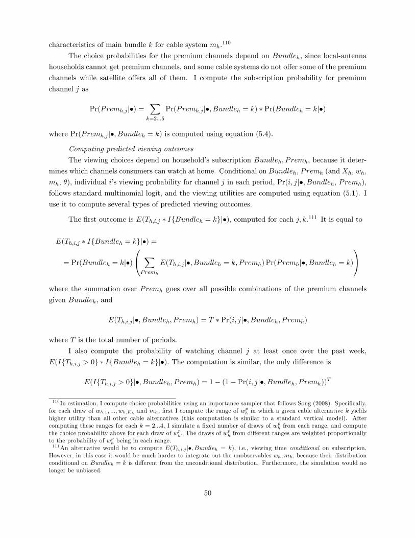
characteristics of main bundle k for cable system mh.110

The choice probabilities for the premium channels depend on Bundleh; since local-antenna

households cannot get premium channels, and some cable systems do not o¤er some of the premium

channels while satellite o¤ers all of them. I compute the subscription probability for premium

channel j as

Pr(Premh;j j) =Xk=2:::5

Pr(Premh;j j; Bundleh = k) Pr(Bundleh = kj)

where Pr(Premh;j j; Bundleh = k) is computed using equation (5.4).

Computing predicted viewing outcomes

The viewing choices depend on households subscription Bundleh; P remh; because it deter-

mines which channels consumers can watch at home. Conditional on Bundleh; P remh (and Xh; wh;

mh; ); individual is viewing probability for channel j in each period, Pr(i; jj; Bundleh; P remh);

follows standard multinomial logit, and the viewing utilities are computed using equation (5.1). I

use it to compute several types of predicted viewing outcomes.

The rst outcome is E(Th;i;j IfBundleh = kgj); computed for each j; k.111 It is equal to

E(Th;i;j IfBundleh = kgj) =

= Pr(Bundleh = kj)

0@ XPremh

E(Th;i;j j; Bundleh = k; Premh) Pr(Premhj; Bundleh = k)

1Awhere the summation over Premh goes over all possible combinations of the premium channels

given Bundleh, and

E(Th;i;j j; Bundleh; P remh) = T Pr(i; jj; Bundleh; P remh)

where T is the total number of periods.

I also compute the probability of watching channel j at least once over the past week,

E(IfTh;i;j > 0g IfBundleh = kgj): The computation is similar, the only di¤erence is

E(IfTh;i;j > 0gj; Bundleh; P remh) = 1 (1 Pr(i; jj; Bundleh; P remh))T

110 In estimation, I compute choice probabilities using an importance sampler that follows Song (2008). Specically,for each draw of wh;1; :::; wh;Kh and mh, rst I compute the range of w

ph in which a given cable alternative k yields

higher utility than all other cable alternatives (this computation is similar to a standard vertical model). Aftercomputing these ranges for each k = 2:::4, I simulate a xed number of draws of wph from each range, and computethe choice probability above for each draw of wph. The draws of w

ph from di¤erent ranges are weighted proportionally

to the probability of wph being in each range.111An alternative would be to compute E(Th;i;j j; Bundleh = k); i.e., viewing time conditional on subscription:However, in this case it would be much harder to integrate out the unobservables wh;mh, because their distributionconditional on Bundleh = k is di¤erent from the unconditional distribution. Furthermore, the simulation would nolonger be unbiased.

50

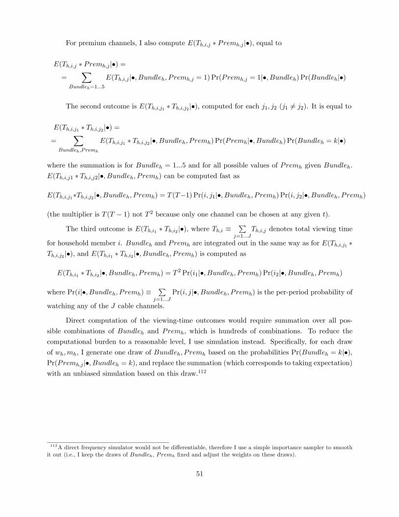
For premium channels, I also compute E(Th;i;j Premh;j j); equal to

E(Th;i;j Premh;j j) =

=X

Bundleh=1:::5

E(Th;i;j j; Bundleh; P remh;j = 1)Pr(Premh;j = 1j; Bundleh) Pr(Bundlehj)

The second outcome is E(Th;i;j1 Th;i;j2 j); computed for each j1; j2 (j1 6= j2). It is equal to

E(Th;i;j1 Th;i;j2 j) =

=X

Bundleh;P remh

E(Th;i;j1 Th;i;j2 j; Bundleh; P remh) Pr(Premhj; Bundleh) Pr(Bundleh = kj)

where the summation is for Bundleh = 1:::5 and for all possible values of Premh given Bundleh.

E(Th;i;j1 Th;i;j2j; Bundleh; P remh) can be computed fast as

E(Th;i;j1Th;i;j2 j; Bundleh; P remh) = T (T1)Pr(i; j1j; Bundleh; P remh) Pr(i; j2j; Bundleh; P remh)

(the multiplier is T (T 1) not T 2 because only one channel can be chosen at any given t):

The third outcome is E(Th;i1 Th;i2 j); where Th;i P

j=1:::J

Th;i;j denotes total viewing time

for household member i. Bundleh and Premh are integrated out in the same way as for E(Th;i;j1 Th;i;j2 j); and E(Th;i1 Th;i2 j; Bundleh; P remh) is computed as

E(Th;i1 Th;i2 j; Bundleh; P remh) = T 2 Pr(i1j; Bundleh; P remh) Pr(i2j; Bundleh; P remh)

where Pr(ij; Bundleh; P remh) P

j=1:::J

Pr(i; jj; Bundleh; P remh) is the per-period probability of

watching any of the J cable channels.

Direct computation of the viewing-time outcomes would require summation over all pos-

sible combinations of Bundleh and Premh; which is hundreds of combinations. To reduce the

computational burden to a reasonable level, I use simulation instead. Specically, for each draw

of wh;mh, I generate one draw of Bundleh; P remh based on the probabilities Pr(Bundleh = kj);Pr(Premh;j j; Bundleh = k); and replace the summation (which corresponds to taking expectation)

with an unbiased simulation based on this draw.112

112A direct frequency simulator would not be di¤erentiable, therefore I use a simple importance sampler to smoothit out (i.e., I keep the draws of Bundleh, Premh xed and adjust the weights on these draws).

51

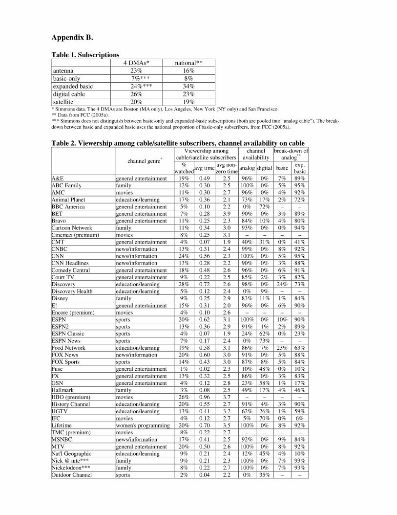
Appendix B.

Table 1. Subscriptions 4 DMAs* national**

antenna 23% 16%

basic-only 7%*** 8%

expanded basic 24%*** 34%

digital cable 26% 23%

satellite 20% 19% * Simmons data. The 4 DMAs are Boston (MA only), Los Angeles, New York (NY only) and San Francisco. ** Data from FCC (2005a). *** Simmons does not distinguish between basic-only and expanded-basic subscriptions (both are pooled into “analog cable”). The break-

down between basic and expanded basic uses the national proportion of basic-only subscribers, from FCC (2005a).

Table 2. Viewership among cable/satellite subscribers, channel availability on cable

Viewership among cable/satellite subscribers

channel availability

break-down of analog**

channel genre* %

watchedavg time

avg non-zero time

analog digital basic exp. basic

A&E general entertainment 19% 0.49 2.5 96% 0% 7% 89%

ABC Family family 12% 0.30 2.5 100% 0% 5% 95%

AMC movies 11% 0.30 2.7 96% 0% 4% 92%

Animal Planet education/learning 17% 0.36 2.1 73% 17% 2% 72%

BBC America general entertainment 5% 0.10 2.2 0% 72% – –

BET general entertainment 7% 0.28 3.9 90% 0% 3% 89%

Bravo general entertainment 11% 0.25 2.3 84% 10% 4% 80%

Cartoon Network family 11% 0.34 3.0 93% 0% 0% 94%

Cinemax (premium) movies 8% 0.25 3.1 – – – –

CMT general entertainment 4% 0.07 1.9 40% 31% 0% 41%

CNBC news/information 13% 0.31 2.4 99% 0% 8% 92%

CNN news/information 24% 0.56 2.3 100% 0% 5% 95%

CNN Headlines news/information 13% 0.28 2.2 90% 0% 3% 88%

Comedy Central general entertainment 18% 0.48 2.6 96% 0% 6% 91%

Court TV general entertainment 9% 0.22 2.5 85% 2% 3% 82%

Discovery education/learning 28% 0.72 2.6 98% 0% 24% 73%

Discovery Health education/learning 5% 0.12 2.4 0% 9% – –

Disney family 9% 0.25 2.9 83% 11% 1% 84%

E! general entertainment 15% 0.31 2.0 96% 0% 6% 90%

Encore (premium) movies 4% 0.10 2.6 – – – –

ESPN sports 20% 0.62 3.1 100% 0% 10% 90%

ESPN2 sports 13% 0.36 2.9 91% 1% 2% 89%

ESPN Classic sports 4% 0.07 1.9 24% 62% 0% 23%

ESPN News sports 7% 0.17 2.4 0% 73% – –

Food Network education/learning 19% 0.58 3.1 86% 7% 23% 63%

FOX News news/information 20% 0.60 3.0 91% 0% 5% 88%

FOX Sports sports 14% 0.43 3.0 87% 8% 5% 84%

Fuse general entertainment 1% 0.02 2.3 10% 48% 0% 10%

FX general entertainment 13% 0.32 2.5 86% 0% 3% 83%

GSN general entertainment 4% 0.12 2.8 23% 58% 1% 17%

Hallmark family 3% 0.08 2.5 49% 17% 4% 46%

HBO (premium) movies 26% 0.96 3.7 – – – –

History Channel education/learning 20% 0.55 2.7 91% 4% 3% 90%

HGTV education/learning 13% 0.41 3.2 62% 26% 1% 59%

IFC movies 4% 0.12 2.7 5% 70% 0% 6%

Lifetime women's programming 20% 0.70 3.5 100% 0% 8% 92%

TMC (premium) movies 8% 0.22 2.7 – – – –

MSNBC news/information 17% 0.41 2.5 92% 0% 9% 84%

MTV general entertainment 20% 0.50 2.6 100% 0% 8% 92%

Nat'l Geographic education/learning 9% 0.21 2.4 12% 45% 4% 10%

Nick @ nite*** family 9% 0.21 2.3 100% 0% 7% 93%

Nickelodeon*** family 8% 0.22 2.7 100% 0% 7% 93%

Outdoor Channel sports 2% 0.04 2.2 0% 35% – –

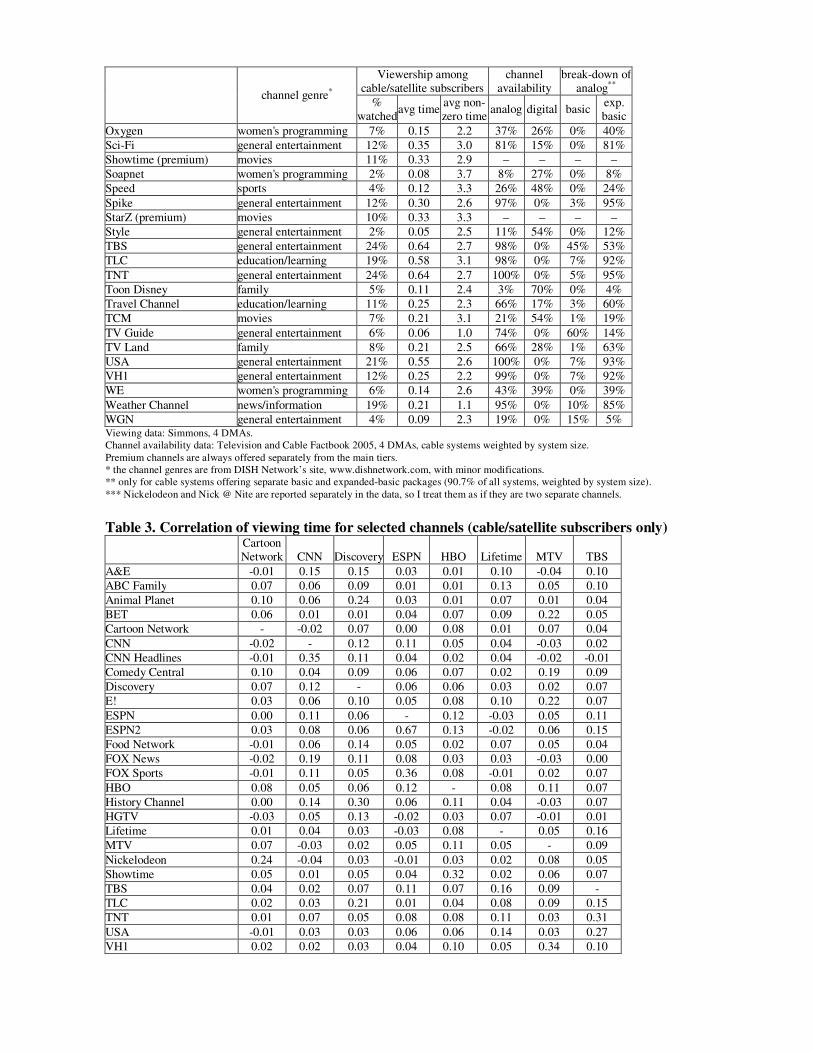
Viewership among cable/satellite subscribers

channel availability

break-down of analog**

channel genre* %

watchedavg time

avg non-zero time

analog digital basic exp. basic

Oxygen women's programming 7% 0.15 2.2 37% 26% 0% 40%

Sci-Fi general entertainment 12% 0.35 3.0 81% 15% 0% 81%

Showtime (premium) movies 11% 0.33 2.9 – – – –

Soapnet women's programming 2% 0.08 3.7 8% 27% 0% 8%

Speed sports 4% 0.12 3.3 26% 48% 0% 24%

Spike general entertainment 12% 0.30 2.6 97% 0% 3% 95%

StarZ (premium) movies 10% 0.33 3.3 – – – –

Style general entertainment 2% 0.05 2.5 11% 54% 0% 12%

TBS general entertainment 24% 0.64 2.7 98% 0% 45% 53%

TLC education/learning 19% 0.58 3.1 98% 0% 7% 92%

TNT general entertainment 24% 0.64 2.7 100% 0% 5% 95%

Toon Disney family 5% 0.11 2.4 3% 70% 0% 4%

Travel Channel education/learning 11% 0.25 2.3 66% 17% 3% 60%

TCM movies 7% 0.21 3.1 21% 54% 1% 19%

TV Guide general entertainment 6% 0.06 1.0 74% 0% 60% 14%

TV Land family 8% 0.21 2.5 66% 28% 1% 63%

USA general entertainment 21% 0.55 2.6 100% 0% 7% 93%

VH1 general entertainment 12% 0.25 2.2 99% 0% 7% 92%

WE women's programming 6% 0.14 2.6 43% 39% 0% 39%

Weather Channel news/information 19% 0.21 1.1 95% 0% 10% 85%

WGN general entertainment 4% 0.09 2.3 19% 0% 15% 5% Viewing data: Simmons, 4 DMAs. Channel availability data: Television and Cable Factbook 2005, 4 DMAs, cable systems weighted by system size.

Premium channels are always offered separately from the main tiers. * the channel genres are from DISH Network’s site, www.dishnetwork.com, with minor modifications. ** only for cable systems offering separate basic and expanded-basic packages (90.7% of all systems, weighted by system size).

*** Nickelodeon and Nick @ Nite are reported separately in the data, so I treat them as if they are two separate channels.

Table 3. Correlation of viewing time for selected channels (cable/satellite subscribers only)

Cartoon Network CNN Discovery ESPN HBO Lifetime MTV TBS

A&E -0.01 0.15 0.15 0.03 0.01 0.10 -0.04 0.10

ABC Family 0.07 0.06 0.09 0.01 0.01 0.13 0.05 0.10

Animal Planet 0.10 0.06 0.24 0.03 0.01 0.07 0.01 0.04

BET 0.06 0.01 0.01 0.04 0.07 0.09 0.22 0.05

Cartoon Network - -0.02 0.07 0.00 0.08 0.01 0.07 0.04

CNN -0.02 - 0.12 0.11 0.05 0.04 -0.03 0.02

CNN Headlines -0.01 0.35 0.11 0.04 0.02 0.04 -0.02 -0.01

Comedy Central 0.10 0.04 0.09 0.06 0.07 0.02 0.19 0.09

Discovery 0.07 0.12 - 0.06 0.06 0.03 0.02 0.07

E! 0.03 0.06 0.10 0.05 0.08 0.10 0.22 0.07

ESPN 0.00 0.11 0.06 - 0.12 -0.03 0.05 0.11

ESPN2 0.03 0.08 0.06 0.67 0.13 -0.02 0.06 0.15

Food Network -0.01 0.06 0.14 0.05 0.02 0.07 0.05 0.04

FOX News -0.02 0.19 0.11 0.08 0.03 0.03 -0.03 0.00

FOX Sports -0.01 0.11 0.05 0.36 0.08 -0.01 0.02 0.07

HBO 0.08 0.05 0.06 0.12 - 0.08 0.11 0.07

History Channel 0.00 0.14 0.30 0.06 0.11 0.04 -0.03 0.07

HGTV -0.03 0.05 0.13 -0.02 0.03 0.07 -0.01 0.01

Lifetime 0.01 0.04 0.03 -0.03 0.08 - 0.05 0.16

MTV 0.07 -0.03 0.02 0.05 0.11 0.05 - 0.09

Nickelodeon 0.24 -0.04 0.03 -0.01 0.03 0.02 0.08 0.05

Showtime 0.05 0.01 0.05 0.04 0.32 0.02 0.06 0.07

TBS 0.04 0.02 0.07 0.11 0.07 0.16 0.09 -

TLC 0.02 0.03 0.21 0.01 0.04 0.08 0.09 0.15

TNT 0.01 0.07 0.05 0.08 0.08 0.11 0.03 0.31

USA -0.01 0.03 0.03 0.06 0.06 0.14 0.03 0.27

VH1 0.02 0.02 0.03 0.04 0.10 0.05 0.34 0.10

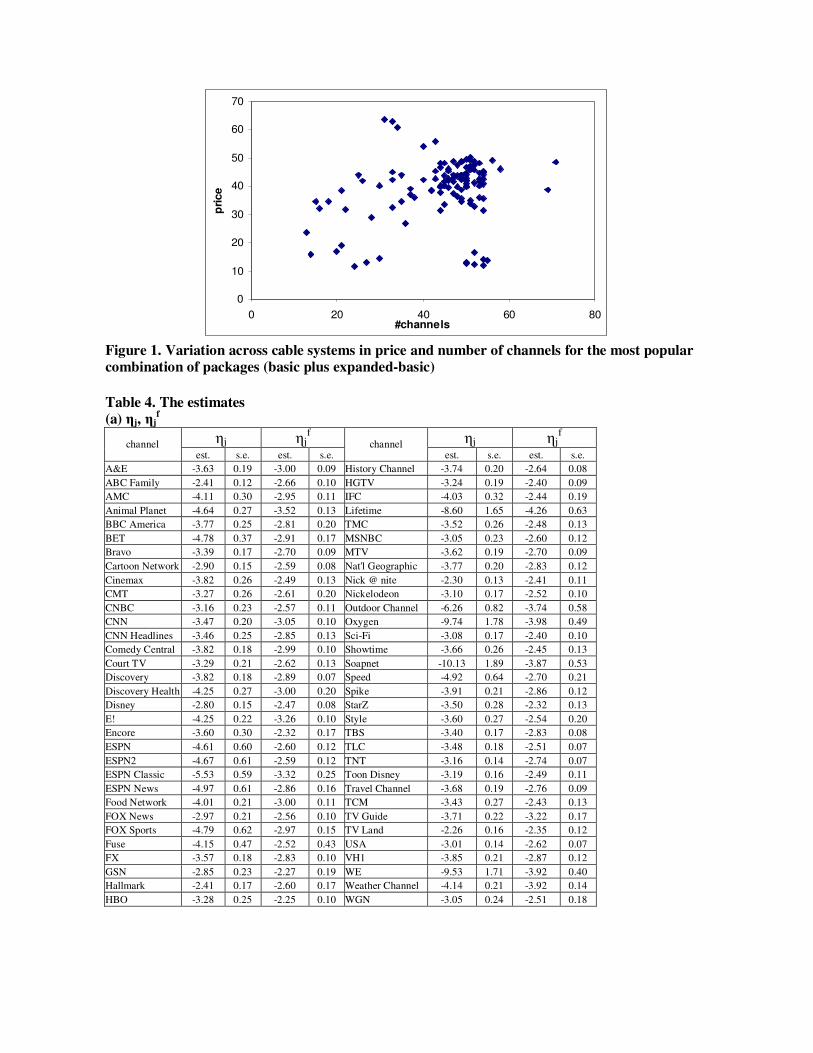
0

10

20

30

40

50

60

70

0 20 40 60 80#channels

pri

ce

Figure 1. Variation across cable systems in price and number of channels for the most popular

combination of packages (basic plus expanded-basic)

Table 4. The estimates

(a) ηj, ηjf

ηj ηjf ηj ηj

f channel

est. s.e. est. s.e. channel

est. s.e. est. s.e.

A&E -3.63 0.19 -3.00 0.09 History Channel -3.74 0.20 -2.64 0.08

ABC Family -2.41 0.12 -2.66 0.10 HGTV -3.24 0.19 -2.40 0.09

AMC -4.11 0.30 -2.95 0.11 IFC -4.03 0.32 -2.44 0.19

Animal Planet -4.64 0.27 -3.52 0.13 Lifetime -8.60 1.65 -4.26 0.63

BBC America -3.77 0.25 -2.81 0.20 TMC -3.52 0.26 -2.48 0.13

BET -4.78 0.37 -2.91 0.17 MSNBC -3.05 0.23 -2.60 0.12

Bravo -3.39 0.17 -2.70 0.09 MTV -3.62 0.19 -2.70 0.09

Cartoon Network -2.90 0.15 -2.59 0.08 Nat'l Geographic -3.77 0.20 -2.83 0.12

Cinemax -3.82 0.26 -2.49 0.13 Nick @ nite -2.30 0.13 -2.41 0.11

CMT -3.27 0.26 -2.61 0.20 Nickelodeon -3.10 0.17 -2.52 0.10

CNBC -3.16 0.23 -2.57 0.11 Outdoor Channel -6.26 0.82 -3.74 0.58

CNN -3.47 0.20 -3.05 0.10 Oxygen -9.74 1.78 -3.98 0.49

CNN Headlines -3.46 0.25 -2.85 0.13 Sci-Fi -3.08 0.17 -2.40 0.10

Comedy Central -3.82 0.18 -2.99 0.10 Showtime -3.66 0.26 -2.45 0.13

Court TV -3.29 0.21 -2.62 0.13 Soapnet -10.13 1.89 -3.87 0.53

Discovery -3.82 0.18 -2.89 0.07 Speed -4.92 0.64 -2.70 0.21

Discovery Health -4.25 0.27 -3.00 0.20 Spike -3.91 0.21 -2.86 0.12

Disney -2.80 0.15 -2.47 0.08 StarZ -3.50 0.28 -2.32 0.13

E! -4.25 0.22 -3.26 0.10 Style -3.60 0.27 -2.54 0.20

Encore -3.60 0.30 -2.32 0.17 TBS -3.40 0.17 -2.83 0.08

ESPN -4.61 0.60 -2.60 0.12 TLC -3.48 0.18 -2.51 0.07

ESPN2 -4.67 0.61 -2.59 0.12 TNT -3.16 0.14 -2.74 0.07

ESPN Classic -5.53 0.59 -3.32 0.25 Toon Disney -3.19 0.16 -2.49 0.11

ESPN News -4.97 0.61 -2.86 0.16 Travel Channel -3.68 0.19 -2.76 0.09

Food Network -4.01 0.21 -3.00 0.11 TCM -3.43 0.27 -2.43 0.13

FOX News -2.97 0.21 -2.56 0.10 TV Guide -3.71 0.22 -3.22 0.17

FOX Sports -4.79 0.62 -2.97 0.15 TV Land -2.26 0.16 -2.35 0.12

Fuse -4.15 0.47 -2.52 0.43 USA -3.01 0.14 -2.62 0.07

FX -3.57 0.18 -2.83 0.10 VH1 -3.85 0.21 -2.87 0.12

GSN -2.85 0.23 -2.27 0.19 WE -9.53 1.71 -3.92 0.40

Hallmark -2.41 0.17 -2.60 0.17 Weather Channel -4.14 0.21 -3.92 0.14

HBO -3.28 0.25 -2.25 0.10 WGN -3.05 0.24 -2.51 0.18

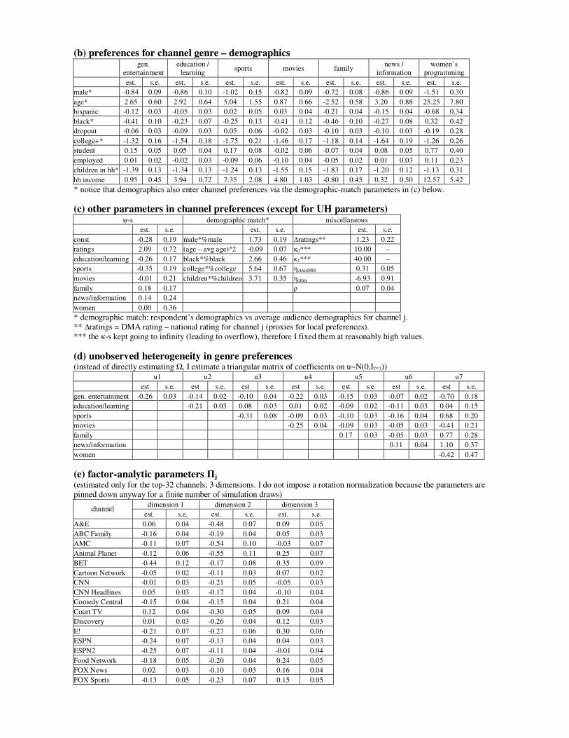
(b) preferences for channel genre – demographics

gen. entertainment

education / learning

sports movies family news /

information women’s

programming

est. s.e. est. s.e. est. s.e. est. s.e. est. s.e. est. s.e. est. s.e.

male* -0.84 0.09 -0.86 0.10 -1.02 0.15 -0.82 0.09 -0.72 0.08 -0.86 0.09 -1.51 0.30

age* 2.65 0.60 2.92 0.64 5.04 1.55 0.87 0.66 -2.52 0.58 3.20 0.88 25.25 7.80

hispanic -0.12 0.03 -0.05 0.03 0.02 0.05 0.03 0.04 -0.21 0.04 -0.15 0.04 -0.68 0.34

black* -0.41 0.10 -0.23 0.07 -0.25 0.13 -0.41 0.12 -0.46 0.10 -0.27 0.08 0.32 0.42

dropout -0.06 0.03 -0.09 0.03 0.05 0.06 -0.02 0.03 -0.10 0.03 -0.10 0.03 -0.19 0.28

college+* -1.32 0.16 -1.54 0.18 -1.75 0.21 -1.46 0.17 -1.18 0.14 -1.64 0.19 -1.26 0.26

student 0.15 0.05 0.05 0.04 0.17 0.08 -0.02 0.06 -0.07 0.04 0.08 0.05 0.77 0.40

employed 0.01 0.02 -0.02 0.03 -0.09 0.06 -0.10 0.04 -0.05 0.02 0.01 0.03 0.11 0.23

children in hh* -1.39 0.13 -1.34 0.13 -1.24 0.13 -1.55 0.15 -1.83 0.17 -1.20 0.12 -1.13 0.31

hh income 0.95 0.45 3.94 0.72 7.35 2.08 4.80 1.03 -0.80 0.45 0.32 0.50 12.57 5.42

* notice that demographics also enter channel preferences via the demographic-match parameters in (c) below.

(c) other parameters in channel preferences (except for UH parameters) ψ-s demographic match* miscellaneous

est. s.e. est. s.e. est. s.e.

const -0.28 0.19 male*%male 1.73 0.19 ∆ratings** 1.23 0.22

ratings 2.09 0.72 (age – avg age)^2 -0.09 0.07 κ0*** 10.00 –

education/learning -0.26 0.17 black*%black 2.66 0.46 κ1*** 40.00 –

sports -0.35 0.19 college*%college 5.64 0.67 ηotherDBS 0.31 0.05

movies -0.01 0.21 children*%children 3.71 0.35 ηother -6.93 0.91

family 0.18 0.17 ρ 0.07 0.04

news/information 0.14 0.24

women 0.00 0.36

* demographic match: respondent’s demographics vs average audience demographics for channel j. ** ∆ratings = DMA rating – national rating for channel j (proxies for local preferences). *** the κ-s kept going to infinity (leading to overflow), therefore I fixed them at reasonably high values.

(d) unobserved heterogeneity in genre preferences (instead of directly estimating Ω, I estimate a triangular matrix of coefficients on u~N(0,I7*7)) u1 u2 u3 u4 u5 u6 u7

est s.e. est s.e. est s.e. est s.e. est s.e. est s.e. est s.e.

gen. entertainment -0.26 0.03 -0.14 0.02 -0.10 0.04 -0.22 0.03 -0.15 0.03 -0.07 0.02 -0.70 0.18

education/learning -0.21 0.03 0.08 0.03 0.01 0.02 -0.09 0.02 -0.11 0.03 0.04 0.15

sports -0.31 0.08 -0.09 0.03 -0.10 0.03 -0.16 0.04 0.68 0.20

movies -0.25 0.04 -0.09 0.03 -0.05 0.03 -0.41 0.21

family 0.17 0.03 -0.05 0.03 0.77 0.28

news/information 0.11 0.04 1.10 0.37

women -0.42 0.47

(e) factor-analytic parameters Пj (estimated only for the top-32 channels, 3 dimensions. I do not impose a rotation normalization because the parameters are pinned down anyway for a finite number of simulation draws)

dimension 1 dimension 2 dimension 3 channel

est. s.e. est. s.e. est. s.e.

A&E 0.06 0.04 -0.48 0.07 0.09 0.05

ABC Family -0.16 0.04 -0.19 0.04 0.05 0.03

AMC -0.11 0.07 -0.54 0.10 -0.03 0.07

Animal Planet -0.12 0.06 -0.55 0.11 0.25 0.07

BET -0.44 0.12 -0.17 0.08 0.35 0.09

Cartoon Network -0.05 0.02 -0.11 0.03 0.07 0.02

CNN -0.01 0.03 -0.21 0.05 -0.05 0.03

CNN Headlines 0.05 0.03 -0.17 0.04 -0.10 0.04

Comedy Central -0.15 0.04 -0.15 0.04 0.21 0.04

Court TV 0.12 0.04 -0.30 0.05 0.09 0.04

Discovery 0.01 0.03 -0.26 0.04 0.12 0.03

E! -0.21 0.07 -0.27 0.06 0.30 0.06

ESPN -0.24 0.07 -0.13 0.04 0.04 0.03

ESPN2 -0.25 0.07 -0.11 0.04 -0.01 0.04

Food Network -0.18 0.05 -0.20 0.04 0.24 0.05

FOX News 0.02 0.03 -0.10 0.03 0.16 0.04

FOX Sports -0.13 0.05 -0.23 0.07 0.15 0.05

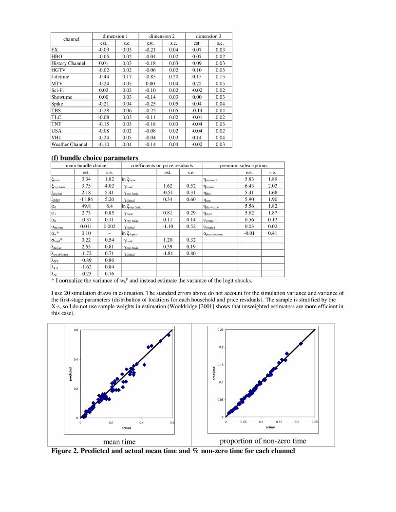
dimension 1 dimension 2 dimension 3 channel

est. s.e. est. s.e. est. s.e.

FX -0.09 0.03 -0.21 0.04 0.07 0.03

HBO -0.05 0.02 -0.04 0.02 0.07 0.02

History Channel 0.01 0.03 -0.18 0.03 0.09 0.03

HGTV -0.02 0.02 -0.06 0.02 0.10 0.03

Lifetime -0.44 0.17 -0.85 0.20 0.15 0.15

MTV -0.24 0.05 0.00 0.04 0.22 0.05

Sci-Fi 0.03 0.03 -0.10 0.02 -0.02 0.02

Showtime 0.00 0.03 -0.14 0.03 0.00 0.03

Spike -0.21 0.04 -0.25 0.05 0.04 0.04

TBS -0.28 0.06 -0.25 0.05 -0.14 0.04

TLC -0.08 0.03 -0.11 0.02 -0.01 0.02

TNT -0.15 0.03 -0.18 0.03 -0.04 0.03

USA -0.08 0.02 -0.08 0.02 -0.04 0.02

VH1 -0.24 0.05 -0.04 0.03 0.14 0.04

Weather Channel -0.10 0.04 -0.14 0.04 -0.02 0.03

(f) bundle choice parameters main bundle choice coefficients on price residuals premium subscriptions

est. s.e. est. s.e. est. s.e.

ξbasic 0.34 1.82 in ξbasic ηcinemax 5.83 1.89

ξexp.basic 3.75 4.02 γbasic 1.62 0.52 ηencore 6.43 2.02

ξdigital 2.18 5.41 γexp.basic -0.51 0.31 ηhbo 5.41 1.68

ξDBS -11.84 5.20 γdigital 0.34 0.60 ηtmc 5.90 1.90

φ0 49.8 8.4 in ξexp.basic ηshowtime 5.56 1.82

φ1 2.73 0.85 γbasic 0.81 0.29 ηstarz 5.62 1.87

α0 -0.37 0.11 γexp.basic 0.11 0.14 φprem,0 0.56 0.12

αincome 0.011 0.002 γdigital -1.10 0.52 φprem,1 0.03 0.02

αw* 0.10 – in ξdigital αprem,income -0.01 0.41

σlogit* 0.22 0.54 γbasic 1.20 0.32

λhouse 2.53 0.81 γexp.basic 0.39 0.19

λownHouse -1.72 0.71 γdigital -1.81 0.80

λNY -0.89 0.86

λLA -1.62 0.84

λSF -0.23 0.76

* I normalize the variance of whp and instead estimate the variance of the logit shocks.

I use 20 simulation draws in estimation. The standard errors above do not account for the simulation variance and variance of the first-stage parameters (distribution of locations for each household and price residuals). The sample is stratified by the X-s, so I do not use sample weights in estimation (Wooldridge [2001] shows that unweighted estimators are more efficient in this case).

0

0.2

0.4

0.6

0 0.2 0.4 0.6

actual

pre

dic

ted

mean time

0

0.05

0.1

0.15

0.2

0.25

0 0.05 0.1 0.15 0.2 0.25

actual

pre

dic

ted

proportion of non-zero time

Figure 2. Predicted and actual mean time and % non-zero time for each channel

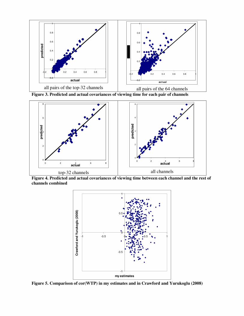
-0.2

0

0.2

0.4

0.6

0.8

1

-0.2 0 0.2 0.4 0.6 0.8 1

actual

pre

dic

ted

all pairs of the top-32 channels

-0.2

0

0.2

0.4

0.6

0.8

1

-0.2 0 0.2 0.4 0.6 0.8 1

actual

all pairs of the 64 channels

Figure 3. Predicted and actual covariances of viewing time for each pair of channels

0

2

4

6

8

0 2 4 6 8

actual

pre

dic

ted

top-32 channels

0

2

4

6

8

0 2 4 6 8

actual

pre

dic

ted

all channels

Figure 4. Predicted and actual covariances of viewing time between each channel and the rest of

channels combined

-1

-0.5

0

0.5

1

-1 -0.5 0 0.5 1

my estimates

Cra

wfo

rd a

nd

Yu

ruk

og

lu (

20

08

)

Figure 5. Comparison of cor(WTP) in my estimates and in Crawford and Yurukoglu (2008)

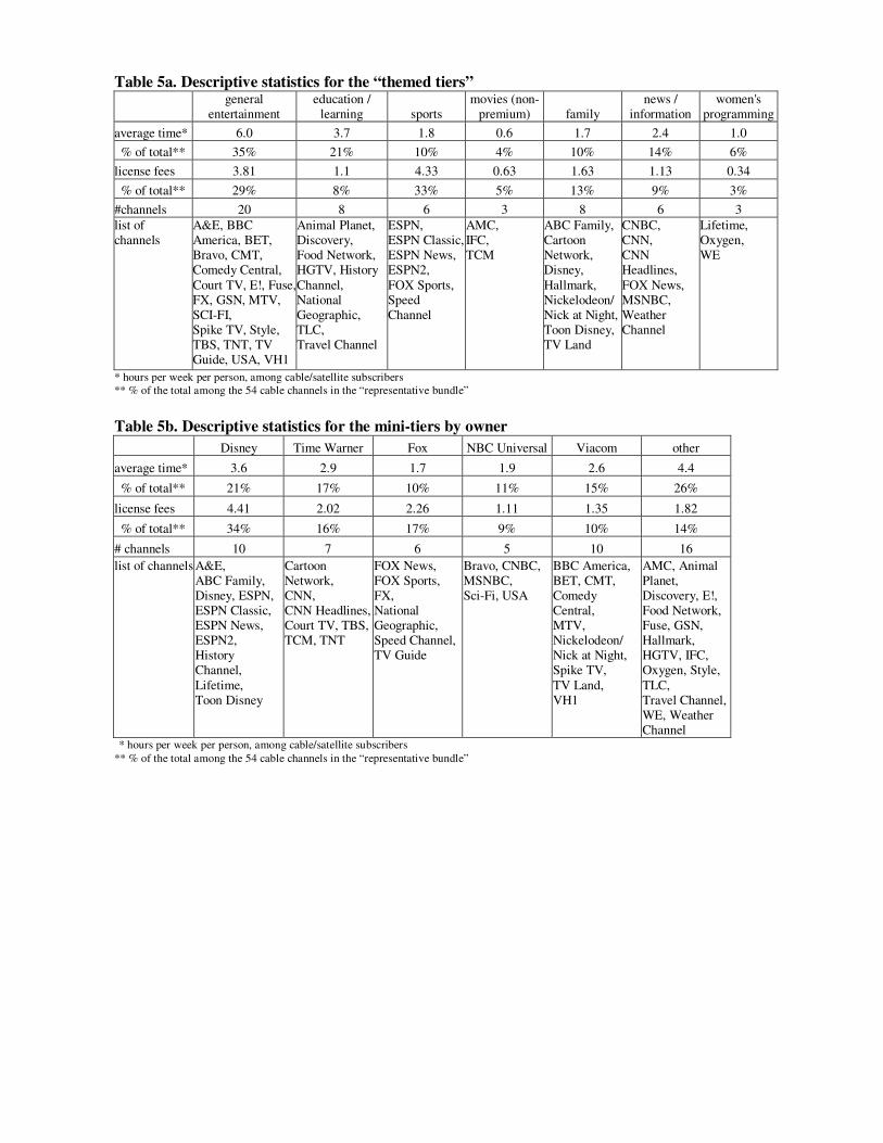
Table 5a. Descriptive statistics for the “themed tiers”

general

entertainment education /

learning sports movies (non-

premium) family news /

information women's

programming

average time* 6.0 3.7 1.8 0.6 1.7 2.4 1.0

% of total** 35% 21% 10% 4% 10% 14% 6%

license fees 3.81 1.1 4.33 0.63 1.63 1.13 0.34

% of total** 29% 8% 33% 5% 13% 9% 3%

#channels 20 8 6 3 8 6 3

list of channels

A&E, BBC America, BET, Bravo, CMT, Comedy Central, Court TV, E!, Fuse, FX, GSN, MTV, SCI-FI, Spike TV, Style, TBS, TNT, TV Guide, USA, VH1

Animal Planet, Discovery, Food Network, HGTV, History Channel, National Geographic, TLC, Travel Channel

ESPN, ESPN Classic, ESPN News, ESPN2, FOX Sports, Speed Channel

AMC, IFC, TCM

ABC Family, Cartoon Network, Disney, Hallmark, Nickelodeon/ Nick at Night, Toon Disney, TV Land

CNBC, CNN, CNN Headlines, FOX News, MSNBC, Weather Channel

Lifetime, Oxygen, WE

* hours per week per person, among cable/satellite subscribers ** % of the total among the 54 cable channels in the “representative bundle”

Table 5b. Descriptive statistics for the mini-tiers by owner

Disney Time Warner Fox NBC Universal Viacom other

average time* 3.6 2.9 1.7 1.9 2.6 4.4

% of total** 21% 17% 10% 11% 15% 26%

license fees 4.41 2.02 2.26 1.11 1.35 1.82

% of total** 34% 16% 17% 9% 10% 14%

# channels 10 7 6 5 10 16

list of channels A&E, ABC Family, Disney, ESPN, ESPN Classic, ESPN News, ESPN2, History Channel, Lifetime, Toon Disney

Cartoon Network, CNN, CNN Headlines, Court TV, TBS, TCM, TNT

FOX News, FOX Sports, FX, National Geographic, Speed Channel, TV Guide

Bravo, CNBC, MSNBC, Sci-Fi, USA

BBC America, BET, CMT, Comedy Central, MTV, Nickelodeon/ Nick at Night, Spike TV, TV Land, VH1

AMC, Animal Planet, Discovery, E!, Food Network, Fuse, GSN, Hallmark, HGTV, IFC, Oxygen, Style, TLC, Travel Channel, WE, Weather Channel

* hours per week per person, among cable/satellite subscribers

** % of the total among the 54 cable channels in the “representative bundle”

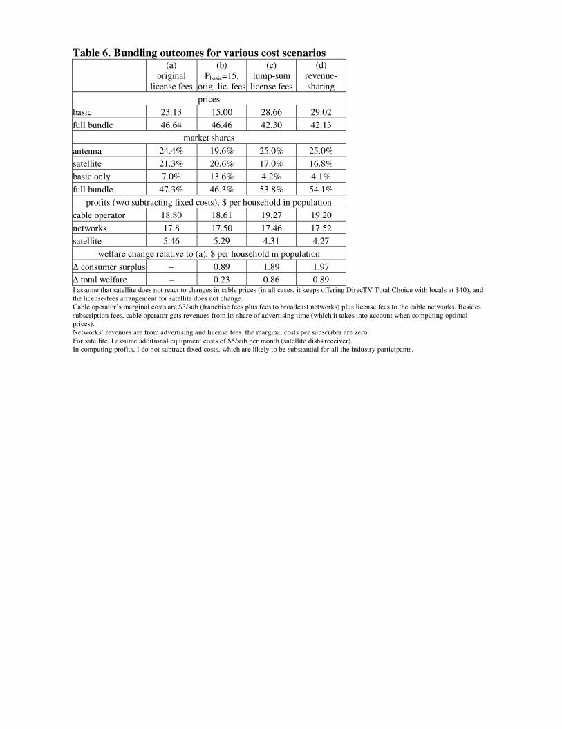
Table 6. Bundling outcomes for various cost scenarios (a)

original license fees

(b) Pbasic=15,

orig. lic. fees

(c) lump-sum

license fees

(d) revenue-sharing

prices

basic 23.13 15.00 28.66 29.02

full bundle 46.64 46.46 42.30 42.13

market shares

antenna 24.4% 19.6% 25.0% 25.0%

satellite 21.3% 20.6% 17.0% 16.8%

basic only 7.0% 13.6% 4.2% 4.1%

full bundle 47.3% 46.3% 53.8% 54.1%

profits (w/o subtracting fixed costs), $ per household in population

cable operator 18.80 18.61 19.27 19.20

networks 17.8 17.50 17.46 17.52

satellite 5.46 5.29 4.31 4.27

welfare change relative to (a), $ per household in population

∆ consumer surplus – 0.89 1.89 1.97

∆ total welfare – 0.23 0.86 0.89 I assume that satellite does not react to changes in cable prices (in all cases, it keeps offering DirecTV Total Choice with locals at $40), and the license-fees arrangement for satellite does not change. Cable operator’s marginal costs are $3/sub (franchise fees plus fees to broadcast networks) plus license fees to the cable networks. Besides

subscription fees, cable operator gets revenues from its share of advertising time (which it takes into account when computing optimal prices). Networks’ revenues are from advertising and license fees, the marginal costs per subscriber are zero.

For satellite, I assume additional equipment costs of $5/sub per month (satellite dish+receiver). In computing profits, I do not subtract fixed costs, which are likely to be substantial for all the industry participants.

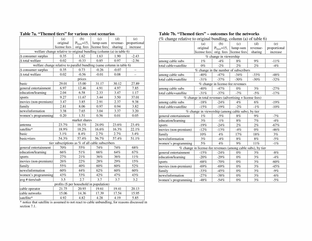
Table 7a. “Themed tiers” for various cost scenarios

(a) original

license fees

(b) Pbasic=15, orig. fees

(c) lump-sum

license fees

(d) revenue-sharing

(e) proportional

increase

welfare change relative to original bundling (column (a) in table 6)

∆ consumer surplus 0.35 1.62 1.63 1.90 -2.43

∆ total welfare 0.02 -0.33 0.85 0.97 -2.56

welfare change relative to parallel bundling (same column in table 6)

∆ consumer surplus 0.35 0.73 -0.26 -0.07 –

∆ total welfare 0.02 -0.56 -0.01 0.08 –

prices

basic 29.01 15.00 31.17 30.12 27.89

general entertainment 6.97 12.46 4.91 4.97 7.85

education/learning 2.04 6.58 2.33 3.47 1.17

sports 9.27 11.67 3.44 3.50 37.01

movies (non-premium) 3.47 3.85 2.91 2.37 9.38

family 2.81 8.06 0.97 0.94 3.82

news/information 3.38 7.65 3.04 3.37 3.20

women’s programming 0.20 1.51 0.56 0.01 0.05

market shares

antenna 23.7% 16.1% 24.0% 23.6% 23.4%

satellite* 18.9% 18.2% 16.6% 16.3% 22.1%

basic 3.1% 8.4% 2.7% 2.7% 3.4%

basic+tiers 54.3% 57.4% 56.7% 57.4% 51.1%

tier subscriptions as % of all cable subscribers

general entertainment 70% 55% 74% 74% 68%

education/learning 66% 51% 66% 64% 67%

sports 27% 21% 36% 36% 11%

movies (non-premium) 26% 22% 28% 29% 15%

family 55% 40% 60% 60% 52%

news/information 60% 44% 62% 60% 60%

women’s programming 43% 33% 42% 47% 43%

avg # tiers/sub 3.5 2.7 3.7 3.7 3.2

profits ($ per household in population)

cable operator 21.75 20.93 19.61 19.41 20.13

cable networks 15.06 14.36 17.39 17.54 15.95

satellite* 4.92 4.82 4.28 4.19 5.85

* notice that satellite is assumed to not react to cable unbundling, for reasons discussed in section 7.1.

Table 7b. “Themed tiers” – outcomes for the networks

(% change relative to original bundling, column (a) of table 6)

(a) original

license fees

(b) Pbasic=15, orig. fees

(c) lump-sum

license fees

(d) revenue-sharing

(e) proportional

increase

% change in viewership

among cable subs 1% -4% 8% 9% -11%

total cable+satellite 0% -2% 2% 2% -4%

% change in the number of subscribers

among cable subs -40% -47% -34% -33% -48%

total cable+satellite -31% -37% -30% -30% -32%

% change in license-fee revenues

among cable subs -40% -47% 0% 3% -27%

total cable+satellite -31% -37% -7% -5% -17%

% change in total revenues (advertising + license fees)

among cable subs -18% -24% 4% 6% -19%

total cable+satellite -15% -19% -2% -1% -10%

% change in viewership (among cable subs), by tier

general entertainment 1% -5% 8% 9% -7%

education/learning 3% -1% 8% 7% -4%

sports -19% -24% 2% 2% -67%

movies (non-premium) -12% -13% -4% 0% -46%

family 10% 4% 17% 18% 3%

news/information 3% -4% 8% 8% -5%

women’s programming 5% 4% 9% 11% -1%

% change in license-fee revenues (among cable subs), by tier

general entertainment -15% -24% 0% 3% -8%

education/learning -20% -29% 0% 3% -4%

sports -68% -70% 0% 3% -60%

movies (non-premium) -69% -69% 0% 3% -45%

family -33% -45% 0% 3% -9%

news/information -27% -38% 0% 3% -6%

women’s programming -48% -54% 0% 3% -5%

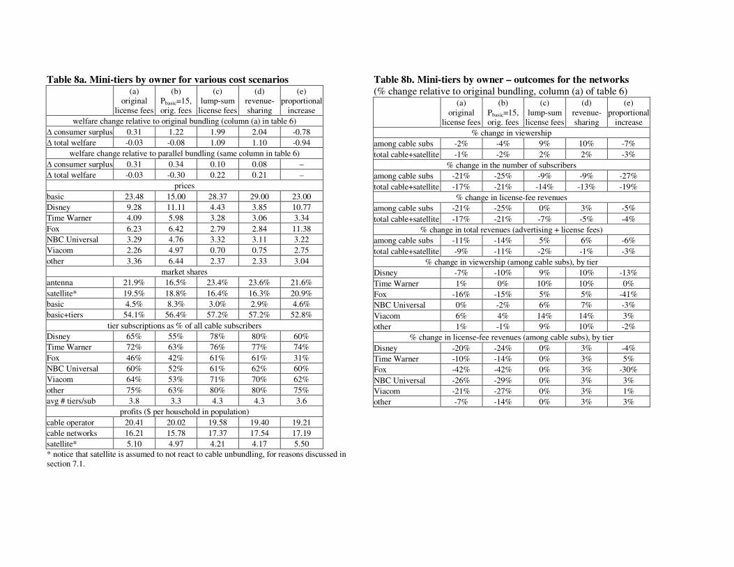
Table 8a. Mini-tiers by owner for various cost scenarios

(a) original

license fees

(b) Pbasic=15, orig. fees

(c) lump-sum

license fees

(d) revenue-sharing

(e) proportional

increase

welfare change relative to original bundling (column (a) in table 6)

∆ consumer surplus 0.31 1.22 1.99 2.04 -0.78

∆ total welfare -0.03 -0.08 1.09 1.10 -0.94

welfare change relative to parallel bundling (same column in table 6)

∆ consumer surplus 0.31 0.34 0.10 0.08 –

∆ total welfare -0.03 -0.30 0.22 0.21 –

prices

basic 23.48 15.00 28.37 29.00 23.00

Disney 9.28 11.11 4.43 3.85 10.77

Time Warner 4.09 5.98 3.28 3.06 3.34

Fox 6.23 6.42 2.79 2.84 11.38

NBC Universal 3.29 4.76 3.32 3.11 3.22

Viacom 2.26 4.97 0.70 0.75 2.75

other 3.36 6.44 2.37 2.33 3.04

market shares

antenna 21.9% 16.5% 23.4% 23.6% 21.6%

satellite* 19.5% 18.8% 16.4% 16.3% 20.9%

basic 4.5% 8.3% 3.0% 2.9% 4.6%

basic+tiers 54.1% 56.4% 57.2% 57.2% 52.8%

tier subscriptions as % of all cable subscribers

Disney 65% 55% 78% 80% 60%

Time Warner 72% 63% 76% 77% 74%

Fox 46% 42% 61% 61% 31%

NBC Universal 60% 52% 61% 62% 60%

Viacom 64% 53% 71% 70% 62%

other 75% 63% 80% 80% 75%

avg # tiers/sub 3.8 3.3 4.3 4.3 3.6

profits ($ per household in population)

cable operator 20.41 20.02 19.58 19.40 19.21

cable networks 16.21 15.78 17.37 17.54 17.19

satellite* 5.10 4.97 4.21 4.17 5.50

* notice that satellite is assumed to not react to cable unbundling, for reasons discussed in section 7.1.

Table 8b. Mini-tiers by owner – outcomes for the networks

(% change relative to original bundling, column (a) of table 6)

(a) original

license fees

(b) Pbasic=15, orig. fees

(c) lump-sum

license fees

(d) revenue-sharing

(e) proportional

increase

% change in viewership

among cable subs -2% -4% 9% 10% -7%

total cable+satellite -1% -2% 2% 2% -3%

% change in the number of subscribers

among cable subs -21% -25% -9% -9% -27%

total cable+satellite -17% -21% -14% -13% -19%

% change in license-fee revenues

among cable subs -21% -25% 0% 3% -5%

total cable+satellite -17% -21% -7% -5% -4%

% change in total revenues (advertising + license fees)

among cable subs -11% -14% 5% 6% -6%

total cable+satellite -9% -11% -2% -1% -3%

% change in viewership (among cable subs), by tier

Disney -7% -10% 9% 10% -13%

Time Warner 1% 0% 10% 10% 0%

Fox -16% -15% 5% 5% -41%

NBC Universal 0% -2% 6% 7% -3%

Viacom 6% 4% 14% 14% 3%

other 1% -1% 9% 10% -2%

% change in license-fee revenues (among cable subs), by tier

Disney -20% -24% 0% 3% -4%

Time Warner -10% -14% 0% 3% 5%

Fox -42% -42% 0% 3% -30%

NBC Universal -26% -29% 0% 3% 3%

Viacom -21% -27% 0% 3% 1%

other -7% -14% 0% 3% 3%