Physics 4BL: Electricity and MagnetismLab Manual

UCLA Department of Physics andAstronomy

Last revision July 11, 2017

1

Introduction

The objective of this course is to teach electricity and magnetism (E&M) by observationsfrom experiments. This approach complements the classroom experience of Physics 1B and1C where you learn the material from lectures and books designed to teach problem solvingskills. Historically, E&M evolved from many observations that called for a theoretical ex-planation. It is a great achievement that all classical E&M phenomena (including Einstein’stheory of special relativity) can be explained by four equations, the so-called Maxwell’sequations. This laboratory course is designed to perform experiments showing the validityof these equations.

In the laboratory, you will have different experiences than in the classroom. In the realworld, there are no point sources, no infinities, all measurements have errors, and sometimesthings don’t work out as expected. A broken instrument or wire can be as frustrating andtime consuming as trying to solve a seemingly impossible homework problem. You will haveto learn patience and persistence to make good measurements.

For solving theoretical problems you first need to learn the appropriate mathematicaltools. For performing experiments you first need to become familiar with measurementtools, called instruments. These include multimeters, oscilloscopes, signal generators, aGaussmeter, digital scale, power supplies and computers. The first lab session is devotedto acquaint you with modern digital data acquisition methods. It is expected that you arealready familiar with basic software such as spreadsheets. In the lab you will save your dataand evaluate the results at home or a computer lab.

Each lab report will have a worksheet portion and a presentation portion (much likephysics 4AL). The worksheet portion will contain brief answers to questions about yourdata taking in the lab. For the presentation portion, some experiments will require onlyparts of a lab report and some will be full reports. A good laboratory report should containa brief but thorough description of your experiment (no need to copy the lab manual),the data obtained (usually in the form of graphs) and evaluations such as line, surfaceand volume integrals, curve fitting, circuit analysis, and any questions raised in the labmanual. The report should be written concisely in a scientific language; it is not an essaywhere you admire the beauty of science or express your frustrations with the equipment.Your TA has no time to read excessively long lab reports; they will be looking for therelevant information and a demonstration of understanding of the results. The reports aredue a week after the experiments have been done.1 Data may be shared with your labpartners unless otherwise specified by this manual or your TA, but the reports (includingfigures, the narrative structure, etc.) must of course be written individually. Copying otherreports constitutes plagiarism and will be reported to the Office of the Dean of Studentswith unpleasant consequences. It is recommended that students bring a personal notebook(electronic or otherwise) to the lab to keep a record of what you did. The lab manual will

1Students taking 4BL in the summer sessions may have sooner deadlines than 7 days. From this pointforward in this manual, the school year schedule will be assumed; summer students should consult their TAsfor the summer deadlines.

2

be asking you questions as you go – you will typically need the answers when you write yourreport, so be sure to record them for your future use.

3

Experiment 1: Circuits

The goal of this lab is for you to become familiar with some of the equipment and techniquesyou will be using this quarter. You will also investigate both simple and more complicatedelectronic circuits. Record your results and the answers to the questions below to use whenyou write your report. There is some linear regression at the end that will be part of this.If you need to review error analysis, please see appendix A, especially propagation of errorsand equation (A.15).

1.1 The Digital Oscilloscope

The oscilloscope is a basic tool in any physics or engineering lab. Modern digital “scopes”sample the input voltage at around 1 GHz, or 1 analog to digital conversion (ADC) everyns. The scope provides its own calibration signal, a 1 kHz, 5 V amplitude square wave. Inthis lab exercise, you will perform three tasks to help familiarize yourself with the scope andits functions.

1.1.1 Calibration Signal

Press the Default Setup button near the top right hand side of the scope (it is one buttondown and in from the right corner). Clip the leads from channel 1 (yellow) to the probecompensation (PROBE COMP) terminals at the lower right corner of the scope. The redclip should connect to the probe compensation terminal (upper), and the black clip shouldconnect to ground (lower). The signal is not steady because the trigger level is set to 0 Vby default. You can fix this by adjusting the trigger level to some small positive voltageusing the Level knob on the right hand side of the scope in the Trigger panel. While you’readjusting it, the trigger level is shown on the screen and the trigger channel and voltage isalways indicated at the bottom right. When the signal is steady, adjust the channel 1 Vertical(i.e. voltage) Scale knob until you can see the whole trace on the scope. You may need tokeep turning up the trigger level to keep the signal steady. What is the voltage amplitudeshown on the scope? The volts per division for channel 1 is indicated at the lower left of thescreen in yellow. The time per division is shown in the lower center of the screen in white.(The manufacturer probably should have programmed this to read “per div.”)

4

If the square wave shows ≈ 50 Vpp (volts peak-to-peak) instead of 5 Vpp, which is whatthat signal should be, it is because the default oscilloscope probe is a 10× attenuating probe.1

We are not using a 10× (times 10) probe but rather a direct, low-resistance connection withno attenuation. From the Ch. 1 menu (yellow 1 button), choose the Probe 10X Voltagesetting, then Attenuation 10X and use the Multipurpose knob to change it from 10X to 1X(push the knob to select the highlighted menu item) so the voltage will display correctly.

1.1.2 Triggering

The trigger indicator is shown at the top center screen as a T in a little orange arrow thatsits above the trigger point on the waveform. Some of the data displayed (to the left of thetrigger indicator) is taken pre-trigger. Note that you are triggering on a rising edge whichlooks pretty steep at this timescale. Turn the Horizontal Scale knob to 1 µs per division. Youwill record two measurements of how long it takes for the pulse to rise to its full value. Firstestimate this value by eye, using the convention that “rise time” means the time requiredfor a digital signal to move from 10% of its maximum value to 90% of its maximum value.Then, using the Measure button on the scope, setup the scope to measure the Rise Time ofCh. 1. These numbers should be fairly close.

Use the Ch. 1 Scale button to change the voltage scale to 5 mV per division. The pre-trigger signal should be close to 0 volts. Estimate the noise or uncertainty in this 0 Vmeasurement. Hit the Single button on the top right hand side a few times to see singletraces. You can also use the Run/Stop button.

1.1.3 Autoset

Another way to set up the scope for an unknown signal is to use the Autoset button. Itanalyzes the signal and sets the trigger and channel gains automatically to display the fullsignal. Try it and note the additional helpful information presented on the screen. (Autosetdoes not change the probe attenuation setting so it may still need to be set manually).

1.2 Potentiometer

A potentiometer, sometimes called a trim pot, a variable resistor, or a voltage divider, is athree-terminal resistor with a knob that can be used to change the resistance between pairsof terminals. They are available with linear or logarithmic knob action. In this lab youwill use a 10-turn, 10 kΩ wirewound linear potentiometer. With one turn of the knob, thesliding connector (often called the “wiper”) moves 1/10 of the way along the wire resistor. Apotentiometer can be thought of as a voltage divider with the wiper tapping into the circuit

1A 10× attenuating probe is a special tool that can be plugged into an oscilloscope and divides the voltageby 10. This is useful not because it reduces the voltage, but because the impedance it presents to the circuitit is probing is higher and it therefore perturbs the behavior of the circuit the less than a lower impedance,particularly at high frequency.

5

between two variable resistors in series whose resistances are related such that their sum isalways a constant (R1 + R2 = Rtotal = constant), as shown in Fig. 1.1. If a voltage source(Vin) were connected to a trim pot as shown in Fig. 1.1(a), what voltage would we read atthe the wiper? Derive an expression for Vout in terms of Vin, R1 and R2.

Figure 1.1: Circuit model of a potentiometer. (a): R1 and R2 are variable resistors whose re-sistances are changed by turning the potentiometer knob. (b): An equivalent representationof this circuit, where the wiper arrow along the side of the resistor indicates that some ofthe resistance is allocated to R1 (above arrow) and some to R2 (below arrow). The diagramon the right is typically how potentiometers are down in circuit diagrams.

The potentiometer you will use in this experiment has 3 leads and a knob on top asshown in Fig. 1.2

You will now investigate how Vout changes as the potentiometer knob position is changed,and determine the functional form of Vout(θ). Here, θ will be the angle through whichthe potentiometer knob has been rotated. To do this, first build the circuit depicted inFig. 1.1(b), with Vin ≈ 5 V coming from the regulated power supply applied to the red andblack jacks (see Appendix D for details of how to use the regulated power supply).

Besides the digital oscilloscope, you will also use a computer based data acquisition(DAQ) system called the myDAQ from National Instruments. The myDAQ also can be usedas a multimeter and function generator.

To use the myDAQ to measure Vout, connect the CH0 red port (the Analog Input AI0+,henceforth called CH0+) on the myDAQ to Vout, and the black port on the potentiometer tothe CH0 black port (CH0-) on the myDAQ. To read the voltages measured by the myDAQ,open the 4BL Application on your computer. Set the Acquisition Modes to measure FixedTime and set the Channel Limits to ±10 V. In this setting, the myDAQ will sample thevoltage every ∆t, which is determined by the number of points and sample rate you choose.Set the number of samples (Number of points to acquire) to 100 points, and use the Scan Ratebar to set the sample rate at 1000 points per second.

6

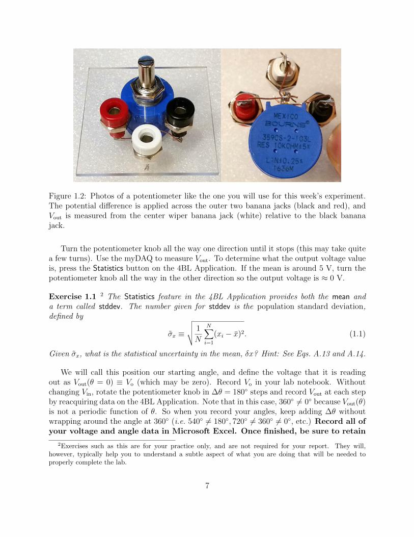
Figure 1.2: Photos of a potentiometer like the one you will use for this week’s experiment.The potential difference is applied across the outer two banana jacks (black and red), andVout is measured from the center wiper banana jack (white) relative to the black bananajack.

Turn the potentiometer knob all the way one direction until it stops (this may take quitea few turns). Use the myDAQ to measure Vout. To determine what the output voltage valueis, press the Statistics button on the 4BL Application. If the mean is around 5 V, turn thepotentiometer knob all the way in the other direction so the output voltage is ≈ 0 V.

Exercise 1.1 2 The Statistics feature in the 4BL Application provides both the mean anda term called stddev. The number given for stddev is the population standard deviation,defined by

σx ≡

√√√√ 1

N

N∑i=1

(xi − x)2. (1.1)

Given σx, what is the statistical uncertainty in the mean, δx? Hint: See Eqs. A.13 and A.14.

We will call this position our starting angle, and define the voltage that it is readingout as Vout(θ = 0) ≡ Vo (which may be zero). Record Vo in your lab notebook. Withoutchanging Vin, rotate the potentiometer knob in ∆θ = 180 steps and record Vout at each stepby reacquiring data on the 4BL Application. Note that in this case, 360 6= 0 because Vout(θ)is not a periodic function of θ. So when you record your angles, keep adding ∆θ withoutwrapping around the angle at 360 (i.e. 540 6= 180, 720 6= 360 6= 0, etc.) Record all ofyour voltage and angle data in Microsoft Excel. Once finished, be sure to retain

2Exercises such as this are for your practice only, and are not required for your report. They will,however, typically help you to understand a subtle aspect of what you are doing that will be needed toproperly complete the lab.

7

the Excel file somehow (email, USB stick, etc.) for your use when writing yourreport. Take note of the data’s form as you collect it. What does the functional form ofVout(θ) seem to look like? For your report, you will need to create a plot of the Vout vs. θdata, perform a linear regression (linear fit), and present the plot with a figure caption andfit line including uncertainties, so be sure to record all of the information you will need tobe able to do this.

1.3 Magnetic Levitator

Next, we will investigate a more complicated circuit that has already been assembled ona printed circuit board (PCB), shown in Fig. 1.3. This circuit is designed to control alevitation apparatus, and you should take a little time to look at it to get a feel for howmany components there are and so forth even though you may not know what the componentsare or what they do. You will not be expected to understand all of the details for how thiscircuit works, but it will provide you with a realistic example of the types of circuits onemight find in useful electronics devices.

1.3.1 Equilibrium

To begin your exploration of the magnetic levitation circuit, at the board, unplug the powercable and the white cable to the copper coil. Detach the magnet from everything and raiseit near the bottom of the coil. At a certain height it is attracted to the steel bolt thatruns through the center of the coil. Below that point, gravity is dominant and it falls. Tryto measure how far below the coil is the equilibrium point? Is the equilibrium stable orunstable?

1.3.2 Infrared LED and Phone Cameras

Plug in board power and the black sensor cable but not the white coil wire. The sensor ismade up of an infrared light-emitting diode (LED) that projects a beam of infrared (IR) light(below the visible red frequency) and a dark IR sensor on the other side whose conductivitychanges with the amount of IR light falling on it. Block the beam with your finger andnotice that the red LED light on the board comes on when the sensor is blocked (if the redLED on the board does not light up, check the wiring and that the plugs are fully inserted,etc.). While one cannot see whether the clear IR emitter is on by eye, many digital camerasare sensitive to IR. If you put a Samsung phone camera in front of the clear LED, you cansee it shining in the IR. Try it, see whether your phone camera is sensitive to IR or has anIR blocking filter installed. Try both the front-facing and rear-facing cameras. Note resultsof your groups phone tests.

8

Figure 1.3: Magnetic levitation PCB. On the left side, a 9 V voltage regulator supplies stableDC voltage to the sensor unit and op amps. On the right side, output from the second opamp controls the coil current through a Darlington transistor pair. The two diodes aroundthe coil drive are designed to protect the circuit from voltage spikes. The coil is inductiveand generates large positive and negative voltage spikes when it is switched on and off bythe transistors.

1.3.3 Levitate

Plug the white coil wire into the board. Now the red LED also indicates when current runsthrough the coil. Place the magnet onto the hex head of the steel bolt (with a nut on thebottom), and hold it with the magnet side up. The energized electromagnet should attractthe magnet. If it repels, flip the magnet over. The idea here is to adjust the sensor so thebottom of the bolt and nut just half blocks the IR beam when the magnet is just below theequilibrium position. You can adjust this by raising or lowering the sensor in its slot, or bylengthening or shortening the bolt assembly by adjusting the nut on the bottom.

9

1.3.4 Feedback Control, PID

This is an example of a feedback (or “servo”) circuit. The position of the bolt assembly issensed and fed back to control the coil current. If the magnet falls and blocks more of thebeam, the coil is turned on to pull it back up. This is called proportional feedback. Afterit reaches the desired height or setpoint, the coil is turned off and the magnet begins tofall again. For stable control though, we don’t want the magnet ping-ponging through thesetpoint. We need some damping so that the velocity is also near 0 when the magnet isnear the setpoint. To add damping we also feedback on the velocity of the bolt assemblywhich is the derivative of the position signal. The faster it is moving, the more importantto damp the motion. In terms of feedback circuits, this is a PD controller, a form of PID(Proportional, Integral, Derivative) controller.

1.3.5 Circuit Description

The circuit diagram in Figure 1.4 shows the magnetic levitation PD controller, and worksapproximately as follows. The sensor signal, which carries the position data, goes to opAmp 1 where it is subtracted from the setpoint voltage connected to the other op amp 1input. The difference between the setpoint and the position sensor, called the error signal, isamplified by op amp 1 and output to where the “magic” happens. There is of course nothingmagical or surprising about a circuit that controls something, but you may agree that thefact that such a simple circuit can levitate something is pretty cool.

The proportional and differential gains are set by the values of the capacitor and resistorin parallel before op amp 2. The voltage appearing across the resistor path (were thereno capacitor in parallel with it) is proportional to the error signal. The voltage appearingacross the capacitor path (in the absence of the parallel resistor) is proportional to thederivative of the error signal and is phase shifted. These two added signals are effectivelyadded together and amplified by op amp 2, whose output is used to control the coil outputtransistors. One way to think about the capacitor is to consider its impedance |Zc| = 1

ωC

where ω is the angular frequency of the signal being analyzed. The capacitor has a very highimpedance (think of it like resistance – it has dimensions of resistance) for low frequency(slow) signals but acts like a short circuit for high frequencies. At about 10 Hz the resistanceand impedance paths are equal, doubling the signal. Signals faster than 10 Hz are boostedeven more by the capacitive path.

1.3.6 Trim pot

Find the trim pot on Figures 1.3 and 1.4. In this circuit the potentiometer is used to fine tunethe position setpoint on op amp 1. The setpoint voltage is determined by the voltage dividermade up of fixed 5 kΩ resistors and a 10 kΩ trim pot. The trim pot voltage is comparedto the sensor signal at op amp 1, and the difference is amplified. The 10 kΩ trimpot is lessthan one turn for full range and adjusts the floating bolt assembly’s height by about 1 mm.

10

Figure 1.4: Diagram of the PD control circuit for magnetic levitation. The proportional andderivative gains are set by the resistor and capacitor in parallel between the op amps (thetriangles called U1A and U1B), labeled “magic happens.” The resistor contributes a voltagedrop across the pair that is proportional to the distance the magnet is from the equilibriumpoint. The capacitor acts as a differentiator, adding the velocity information with a phaseshift. This differential term adds necessary damping, so that the magnet slows to a stopnear the equilibrium setpoint instead of overshooting.

1.4 Lab Report

Your lab report this week (like most weeks) will consist of two parts – a worksheet and apresentation report. These will be two parts of a single document that you will turn in onTurnItIn, nominally 7 days after the start of your lab section.3

The worksheet will consist of a series of questions intended to be answered essentially inlist form in the first part of your report. Please use the numering and lettering scheme shownand answer in complete sentences so that your grader knows which question you’re answering(some parts have more than one question). For this experiment’s report, the worksheet willcount for 40% of the score and the presentation report will count for 60% of the score forthe report.

1.4.1 Worksheet

1. Oscilloscope

(a) What is the measured amplitude of the scope’s calibration signal? (Be sure totake any scope attenuation into account to report the real voltage of the signal.)

3Please consult your TA to learn the actual due date, particularly if you are taking this course in thesummer.

11

(b) What is the risetime of the calibration signal as measured by eye? What is itwhen using the risetime measure function on the scope?

(c) Estimate the uncertainty in the ≈ 0 V signal from the pre-triggered portion ofthe signal.

2. Potentiometer and myDAQ

(a) Derive an expression for Vout on the potentiometer wiper as a function of the inputvoltage, R1, and R2 (Fig. 1.1(a)).

(b) What was the voltage you applied across the potentiometer?

(c) What is the apparent functional form of the potentiometer’s output voltage as afunction of the turning angle θ?

(d) Is the potentiometer Ohmic (does it follow Ohm’s Law, V = IR)?

3. Magnetic Levitator

(a) About how far below the magnetic coil is the equilibrium position of the boltassembly (measured to the top of the magnet on top)?

(b) Is this equilibrium stable or unstable? How can you tell?

(c) Which cell phone cameras (if any) in your group were sensitive to the IR light?

1.4.2 Presentation Report

Using the data you saved in Excel, you will determine how the potentiometer’s outputvoltage depends on the angle through which the control knob has turned. Additionally, youwill calculate what is called the ndependent linearity of the potentiometer to compare to themanufacturer’s claim. You can find this rating listed on the bottom of the potentiometer inFig. 1.2.

The way you will present this analysis in your presentation report this week is by pre-senting it as two, separate plots on separate pages with figure captions and a little bit ofbody text. The guidelines for making figures were covered in Physics 4AL, and you mayconsult the lab manual4 from that course (typically found on Prof. Campbell’s homepage)for guidelines if you need a refresher.

Briefly, you will need to:

1. Create a raw data plot

• In Excel, place all your output voltage data in one column, and their correspondingθ values in the column to the right. You do not need to present this step in yourreport.

4Specifically, §2.3.3

12

• Create a scatter plot of all the Vout vs. θ data, and run a linear regression on thedata as well. Present your plot the fit line on the same graph as the data on adedicated page in your labreport.

• Provide a formal figure caption below the plot as per the Physics 4AL manualthat includes the results of your linear regression.

• In a sentence or two of body text below the figure caption, discuss the significanceof the intercept and slope of the fit line.

2. Independent linearity calculation

• Plot the normalized output voltage Vout/Vin vs. θ and run a linear regression toget the fit parameters with uncertainties. Present this plot on a dedicated pagein your report with a proper figure caption that includes the results of your fit.

• In a separate column, calculate the differences between the normalized voltage ofeach data point and the value of the normalized voltage given by the fit line forthat θ. These differences are called the “residuals” of the fit. This means if thefit line is y(x) = mx + b, for each x value, calculate the difference between whatthe fit line produces y(x) and what was observed in the lab (a single y data pointassociated with that x). You do not need to present this step in your report.

• Find the minimum and maximum of the absolute values of the residuals. Then,calculate the maximum and minimum percentage deviation from the fit line withrespect to the applied voltage (% deviation = (deviation×100)/Vin). Below yourplot, provide a few sentences of body text describing this analysis, includinganswers to the following item (below).

• The manufacturing company claims a maximum tolerable independent linearityof ±0.25%. Do your results fall within this tolerance range? What does this sayabout the potentiometer you used?

13

Experiment 2: Lorentz Force

2.1 Background

In 1897, J.J. Thomson discovered the electron and measured its charge to mass ratio, e/m[7]. The electron was the first sub-atomic and first elementary particle discovered. You willrepeat this Nobel Prize winning experiment as part of today’s lab and write a report onyour findings. Measuring e/m makes use of the Lorentz Force on a particle with charge qtraveling at velocity v through magnetic field B.

F = qE + qv ×B (2.1)

The magnetic part for electrons Fe,mag. = −e(v×B) is notable in the sense that the forcevector is not along the line connecting two charges or masses, but rather is perpendicularto both the electron velocity and the direction of the magnetic field. Use the right handrule to figure out the direction of the force. If the magnetic field is strong enough to bendthe beam into a circle with radius R, we can equate the magnetic force to the centripetalforce required for uniform circular motion Fe,mag. = mv2/R. If the geometry is such that theelectron velocity is always perpendicular to the magnetic field,

evB =mv2

R(2.2)

From this we can measure the charge to mass ratio of the electron, e/m. See Figure 2.1and use the right-hand-rule to check that the direction of the magnetic force is indeed in thedirection required for uniform circular motion.

2.1.1 Cathode Ray Tube and Electron Gun

The apparatus you will use in this experiment is a form of cathode ray vacuum tube (CRT).The electron beam, or cathode ray [7], is created by an electron gun shown in Figure 2.2.Electrons are essentially boiled off a glowing filament called the cathode. After making surethat the DEFLECTING VOLTAGE switch is OFF and the knob is turned to 0 V, the VOLTAGECONTROL knob is turned to 0 V, the MAGNETIZING CURRENT switch is OFF and the knobis turned all the way down, turn on the CRT using the POWER switch. Look behind theelectron gun from the side and you will see the glowing filament.

14

Figure 2.1: An electron beam bent into a clockwise circular trajectory by a magnetic field.The metal electron gun at the bottom produces a narrow beam of electrons with energyeV , where V is the acceleration voltage. There is a uniform magnetic field into the page.The magnetic part of the Lorentz force produces a centripetal acceleration, bending theelectron path into a circle. The electrons can not be seen but their trajectory is made visibleby a small amount of mercury vapor in the evacuated tube. Some of the electrons collideinelastically with mercury atoms, exciting them to emit light.

An anode biased a few hundred volts (V ) positive relative to the cathode pulls electronsfrom the cathode and accelerates them in one direction. The electrons emerge from an aper-ture in the anode with a kinetic energy equal to eV or below. Electrons are not visibledirectly, but they can scatter from and excite the low pressure mercury gas in the tube. Tosee the electrons emerging, slowly turn up the VOLTAGE CONTROL knob for ACCELERAT-ING VOLTAGE while looking at the conical end of the anode. When the ACCELERATINGVOLTAGE reaches about 80 V, you will begin to see a little blue glow from the atoms thatare being excited through electron impact excitation. The glowing volume is essentially atracer showing where the electrons are. When you are done, turn down the ACCELERATINGVOLTAGE to 0 V.

The electron beam can be deflected by electric and magnetic fields. Our e-gun has twodeflection plates in front of the anode aperture, shown in Fig. 2.1 and 2.2. Find the deflection

15

Figure 2.2: The electron gun for this experiment uses thermionic emission and an electricfield between the anode and cathode to produce a narrow beam of electrons with energy eV .Our electron gun also has electrostatic deflection plates in front of the cathode that can beused to create a vertical electric field.

plates in your CRT and try to figure out the electric field direction at the aperture if theDEFLECTING VOLTAGE in POSITIVE mode applies the knob voltage to the top plate relativeto the bottom plate. What direction is the electric field at the beam in this case? Withoutelectric or magnetic fields, the beam will follow a straight path and hit the glass. Don’tallow the beam to hit the same spot on the glass for many minutes at a time –it can drill a small hole and destroy the vacuum in the tube. Turn on the electronbeam again and experiment with the DEFLECTING VOLTAGE. This was how old televisionsused to work! Turn off the electron beam and deflection plate voltages when you are done.

Next, we will study the effect of a magnetic field on the electron beam trajectory. First,with the electron beam off, turn up the MAGNETIZING CURRENT to the two large coils toabout 1 A by turning the CURRENT CONTROL knob and switch clockwise. Then turn upthe beam accelerating voltage until the beam appears. Use the right hand rule to figure outthe direction of the magnetic field at the location of the beam. Note qualitatively how theradius of the beam changes with accelerating voltage and magnetizing current.

Next, grasp the tube at the bottom plastic base and carefully rotate it in its socket.Describe the electron beam motion in your notebook. Discuss how this motion follows fromthe Lorentz force equation. The initial velocity of the electron beam can be described as

16

having components along the magnetic field and components perpendicular to the field,v = v‖ + v⊥. Align the tube so that the circle lies in a plane perpendicular to the magneticfield, v‖ = 0. This alignment is important for the measurements to follow.

For your own notes, starting from evB = mv2/R, show that if V is the acceleratingvoltage,

e

m=

2V

B2R2. (2.3)

2.1.2 Helmholtz Coils

In order to measure e/m, you will apply a uniform, static magnetic field to the electrons.The magnetic field strength is controlled by the current (I) to two large coils. The geometryof these coils is carefully chosen to create a uniform magnetic field over the path of theelectron beam. The configuration we will employ to optimize the uniformity of the fieldin the midplane uses two, coaxial identical coils of radius Rc spaced a distance Rc apart,which is called a Helmholtz configuration (or simply “Helmholtz coils”). The magnetic fieldmagnitude at the center is then given by 1

B =8µ0IN

5√

5Rc

(2.4)

where N is the number of windings in each coil. For your calculations, you may assume ourcoils have a radius of Rc = (0.140± 0.002) m and N = 150.00± 0.01 turns.

Helmholtz coils are widely used in sensitive experiments to cancel stray, uniform fieldssuch as the earth’s magnetic field. Three orthogonal pairs can create or cancel fields in anydirection. Should we be worried about the earth’s field in our measurement of e/m? Theearth’s field is about 0.5 gauss, or 50 µT.

2.1.3 Measurement of e/m

Find an expression for e/m in terms of the accelerating voltage V , the coil current I and thetrajectory radius R. The general idea is to set the acceleration voltage and the coil currentto known values and then measure the radius of the electron beam’s trajectory. Develop aplan to take data for at least 9 different settings that cover the range between 100 to 200 Vand 1 and 2 A. Each person should make at least two measurements, but you will eachanalyze all 9. The key to making a good measurement is overcoming parallax in the radiusmeasurement. One way to do this is to fix the ruler at the correct height and to positionyour eye directly in front of the left side of the beam. Slide the index to the left side of

1Deriving the relationship between the radius of the coils and their optimal distance apart for the mostuniform field in the center is a common homework or exam problem. We start from the Biot-Savart law

for the magnetic field on axis, a distance x away from a current loop of radius Rc, B =µ0INR

2c

2(x2+R2c)

3/2 . Using

superposition, we can write the field in the center when the coils are 2x away from each other. To optimizethe field, the gradient and the curvature, the first and second derivatives of B with respect to x will vanishat a particular distance xH = Rc/2.

17

the arc and sight down the groove in the top of the index. Read the scale and then repeaton the right side to the right edge. The difference divided by 2 is the radius. Record thevoltage, current, and radius. Use multimeters connected to the banana jacks on the back foraccurate measurements. Make sure the multimeters are set up correctly to make the voltageor current measurement and that the range is correct. If the meters aren’t set correctly,they can effect the performance of the CRT. For each set of values of V , I, and R, youwill calculate e/m. This week’s presentation report will be a very short lab report on yourmeasurement of e/m, so please be sure to gather all of the information you will want laterwhen you are writing this report.

2.2 Diodes and transformers

A common laboratory problem is the need to design an appropriate DC power supply for agiven circuit. Typical electronic circuits operate at a low voltage (< 50 V), and require directcurrent (DC). The wall plug, however, provides “120 VAC”, 60 Hz AC (alternating current),which is typically well-approximated as a sine wave (whose amplitude is not 120 V!) witha cyclic frequency of f = 60 Hz2. For example, the Lorentz force apparatus has at leastthree power supplies. Starting with 120 VAC from the wall plug, it generates 6.3 V for thefilament current, low voltage DC current for the Helmholtz coils, and up to 250 V DC forthe accelerating voltage. For the rest of this lab you will investigate circuits that can be usedto change voltages and convert AC to DC. Observations should go in your lab notebook andwill not be part of the presentation report, but will be useful for this week’s worksheet.

The first step in making a DC supply is usually a transformer. In this part of the labwe use a step-down transformer that converts 120 VAC to 12 VAC. Find the transformer ina black case on the lab bench, unplug it, and take off the top so you can inspect it. Mosttransformers have two coils, a primary and a secondary. The primary coil plugs into thewall and handles the full 120 VAC. The secondary coil connects to the output. Find theprimary and secondary coils on this transformer. They are wrapped around a laminated ironcore to duct all the magnetic flux from the primary to the secondary. The output voltage isdetermined by the turn ratio of the coils, Vout =

Nsecondary

NprimaryVin. Read the removable top of the

transformer. It gives information about the transformer input and output and how muchpower the primary and secondary can handle before melting. We are using a 1 A fuse and a1 kΩ resistor in series on the secondary to protect the transformer and circuit.

Connect a 5 kΩ resistor across the output wires, plug in the transformer, and read thevoltage across the resistor on the oscilloscope. Set the scope to trigger off the AC line. Notethe voltage and other characteristics of the signal in your lab notebook and compare to thelabel on the transformer. If you find the results of your measurement puzzling, considerwhat the RMS (root mean square, i.e. the square root of the one-cycle average of the squareof the voltage) voltage would be.

2Part of what you will be exploring in this experiment is what “120 VAC” really means (that is, whatthe amplitude of such a signal is), and the answer may surprise you.

18

Figure 2.3: The orientation of a diode and the diode symbol. The white band on the physicaldiode (bottom) is the cathode end, which you can remember as matching up with the littleline on the end of the diode symbol arrow (top). An ideal diode only conducts current whenthe anode end is at least a “diode drop” higher than the cathode end.

Next add a single diode (Figure 2.3) to the circuit between the fuse holder and the resistoras shown at the top of Figure 2.4. Again, use the oscilloscope to observe the voltage acrossthe resistor on the scope and draw the waveform for your notes, along with quantitativeinformation such as the amplitude. Try switching the direction of the diode and see whathappens. Diodes are non-Ohmic circuit elements that conduct primarily in one direction(the forward bias), and block current in the other direction (the reverse bias). This behavioris called rectification and can be used to convert AC to DC. The voltage drop across a diodewhen conducting is called the “diode drop.” It is typically about 0.6-0.7 V for silicon diodes.

Figure 2.4: Two ways to convert Alternating Current (AC) to Direct Current (DC). Thetop shows half-wave rectification achieved with a single diode. The bottom shows full-waverectification achieved with four diodes

The next step is to build the full-wave rectifier shown at the bottom of Figure 2.4 (or2.5). There is a clear, plastic board at your station if you would like to lay out the circuit byplacing components into the holes in the desired orientation before connecting the elementstogether. After you have the correct waveform shown in the figure, trace out how the current

19

Figure 2.5: A simple DC power supply using a diode bridge. The diodes are wired the sameas the bottom of Figure 2.4, just drawn differently.

flows in this circuit for the cases where the top of the transformer is positive or negative.The top of the resistor should always be positive with respect to the bottom of the resistor.Again take notes on the waveform you see on the oscilloscope.

Finally, add the 47 µF electrolytic capacitor in parallel with the 5kΩ resistor as shown inFigure 2.5 and record what you see on the scope. Be careful while doing this, becauseelectrolytic capacitors are polarized and can explode if enough voltage is appliedin the wrong direction. The white band with arrows shows the negative terminal of thecapacitor. Make sure the negative lead is connected to the negative side of the diode bridge.You should see a constant DC voltage with a ripple on top. Record your observations aboutthe waveform, including the DC level and the magnitude of the ripple. When done, unplugthe transformer and return the circuit elements into their proper location.

2.3 Lab Report

This week’s worksheet with cover both the e/m measurement and the diode experiment, andwill be worth 50% of your report score. The other 50% will come from your presentationreport on the e/m measurement.

2.3.1 Worksheet

1. Measurement of e/m

(a) When the electron beam is bent into a circle, what is the direction of the magneticfield at the location of the beam?

(b) Qualitatively, how does the radius of the beam change with accelerating voltageand magnetizing current?

(c) Describe the shape of the electron beam trajectories when the magnetic field is notperpendicular to the electron velocity. How does it follow from the Lorentz forceequation when the velocity of the electrons have components along the magneticfield and components perpendicular to the field, v = v‖ + v⊥ ?

20

(d) Starting from evB = mv2/R show that if V is the accelerating voltage, em

= 2VB2R2 .

2. Diodes

(a) What is the transformer secondary signal compared to voltage rating? Calculatethe RMS voltage of this signal (assuming it to be a sine wave) and compare thatto the voltage rating.

(b) Record the DC level and the magnitude of the ripple for the full-wave rectifierDC power supply you built.

2.3.2 Presentation Report

For the presentation report, you are tasked with presenting data before and after manipu-lation, and explaining important results. Additionally, you must introduce the experiment,explain the experimental setup and data collected, analyze the data, and draw conclusionsfrom the numerical analysis.

1. Cover Sheet (this will come before even the worksheet)

• Experiment number and title

• your name and UID

• the date the lab was performed

• your lab section (for instance, “Tuesday 2pm”)

• your TA’s name

• “Lab Partner(s):” followed by your lab partners’ names

2. Introduction The introduction section explains the purpose of your experiment andhow you will demonstrate this purpose. Try to be as brief as possible, yet still get yourpoint across.

3. Experimental Description and Results This section should briefly explain whatwas measured and how the data were collected (diagrams of the experimental setupmay be helpful) and present the raw data in graphical form (if appropriate), includinguncertainty values with all numbers. Your graphs should of course include labels onboth axes that include units, etc. (see the Physics 4AL manual, §2.3.3 for guidelines).Label your graphs as Figure 1, Figure 2, etc, in the caption so that you can refer tothem in your text. In the text, explain the meaning of the variables on both axesand include an explanation that makes it clear to the reader how to interpret theinformation displayed on in the plots.

Along with a description of the experimental setup, your report should contain:

• A table of experimentally relevant values (Vaccel, Icoils, electron beam radii R, e/mvalues)

21

• A plot of Vaccel as a function of B2R2/2.

4. Analysis This section should present any calculations performed on the raw data,including uncertainties using propagation of errors (although this calculation need notbe shown if it is straightforward). For example, if you were testing Ohm’s law and youmeasured V and R, then here you would calculate I. If you have a theoretical value foryour calculated quantity (I in this example), state whether or not it is in agreementwith your measurement (i.e. within your uncertainty range).

This section should include:

• Experimental measured value of e/m from each of your 9 individual measurementswith uncertainties. Combine these into one mean value with an appropriate un-certainty and state this as the result of your first method.

• Results of linear regression of Vaccel as a function of B2R2/2, which will be theresult of your second method for measuring this quantity.

• Compare the two methods for determining e/m. Which is more accurate?

5. Conclusion

State how your results demonstrate (or fail to demonstrate) the objectives you pre-sented in the introduction section.

22

Experiment 3: AC Circuits

3.1 Background Information

As opposed to DC currents (or voltages), which take a single, static value, AC currents canvary in amplitude, frequency, and phase. When analyzing circuitry for AC behavior, thecurrent (or voltage) is often modeled as a sine wave of unknown frequency ω, and referredto as a signal. DC can often be thought of a zero frequency signal (ω→ 0), which reducesthe DC behavior to a special case of the AC analysis.

In this laboratory exercise you will examine some basic properties of AC circuits. You willinvestigate the transient state behavior of RC and RL series circuits, as well as a resonantRLC circuit. Since the performance of an AC circuit is generally frequency dependent, thisrequires a generalization of the idea of resistance called impedance.

3.1.1 AC Circuits

One way to create an AC circuit is to connect a circuit element to a voltage source thatvaries in time, causing a current to be driven that alternates in direction with time (of-ten sinusoidally, but not necessarily). In addition to the resistive components studied lastweek, for AC circuits is it important to consider reactive components such as capacitors andinductors.

Capacitors

Conceptually, a capacitor can be thought of as a pair of plates that are spaced apart fromone another by an insulating material. The capacitance (C) of a capacitor specifies the ratioof the charge on each plate (Q) per unit voltage difference between the two plates (V ):

C =Q

V. (3.1)

The SI unit of measure for capacitance is the farad (F), and this property is independentof frequency. Differentiating Eq. 3.1 with respect to time yields an equation that relates thecurrent through the capacitor (I) to the voltage applied:

23

I =dQ

dt= C

dV

dt. (3.2)

From this, we see that current flows through a capacitor only when the voltage across it variesin time. Thus, if we were to connect a a capacitor to a DC battery, no current would flow inthe steady state because the capacitor would act as an open circuit. However, current wouldflow initially since at the instant the capacitor was connected to the battery, the voltagewould change rapidly from zero volts to the voltage of the battery.

Now consider a circuit with a resistor and capacitor in series, called an RC circuit,connected to a battery as shown in Fig. 3.2. At the instant the circuit gets connectedto the battery, dV/dt will be large and the capacitor therefore won’t impede the currentflow. The current flow in this case is impeded only by the resistor, and the voltage dropacross the resistor will be the full battery voltage. After a certain amount of time, thevoltage across the capacitor will settle to a constant value (the voltage of the battery), withQ(t) = Qo = constant, and no more current will flow (in accordance with Eq. 3.2). In thisstate, current flow is impeded by the capacitor, and thus the full voltage of the battery isacross the capacitor and there will be no voltage drop across the resistor. This sequence iscalled charging the capacitor.

The initial response of the RC circuit where the current is flowing is called the transientstate period, and the period when the current stops flowing is called the steady state period.There is a a characteristic time for the transition between these two periods called the RCtime constant. By using Kirchhoff’s law, Ohm’s law, and Eq. 3.1 we can derive the voltageas a function of time across the capacitor:

VC(t) = Vb(1− e−t/RC

), (3.3)

where Vb is the voltage of the battery and we have assumed that t = 0 is the instant whenthe circuit is connected to the battery. This equation defines the timescale of transitionbetween the transient and the steady state in an RC circuit,

τ ≡ RC. (3.4)

Inductors

The other reactive component we will be studying in this experiment is is called an inductor.Inductors are characterized by their inductance (L), which is also a frequency-independentquantity and satisfies the relation

V = LdI

dt. (3.5)

The SI unit for inductance is the henry (H).Equation 3.5 shows us that the voltage across an inductor is large when we have a rapidly

changing current. Thus, if we form a circuit with a resistor and inductor in series (calledan RL circuit) and connect this circuit to a battery at time t = 0, we will again have atransient period and a steady state period. During the transient period, the current will

24

rapidly increase from zero (when the circuit is disconnected from the battery, Iinitial = 0)to its maximum current. During this period, dI/dt is large, and thus the entire voltage isdropped across the inductor. When the current reaches steady state, it is impeded by onlythe resistor and thus the entire voltage drop is across the resistor. We can use Kirchoff’slaw, Ohm’s law, and Eq. 3.5 to derive the voltage across the inductor as a function of time:

VL(t) = Vbe−tR/L. (3.6)

This equation defines the timescale of the transition between the transient and steady stateperiods in an RL circuit,

τ ≡ L

R. (3.7)

Note that when t = τ , we should expect VL (τ) = Vb/e, which is why we often call τ the“one over e folding time.” It can be shown via Kirchoff’s laws, Ohm’s law, and Lenz’s lawthat the current through the inductor in an RL circuit is of the form

IL(t) =VbR

(1− e−t/τ ). (3.8)

If this current will be measured by measuring the voltage drop across the resistor in serieswith the inductor, it may be more instructive to write this as

VR(t) = Vb(1− e−t/τ ). (3.9)

In the first part of this experiment, you will build an RC circuit and measure the voltageduring the transient time period, then do the same for the current in an RL circuit, comparingyour results to equations 3.3 and 3.6. In the second part of the experiment, you will buildwhat’s called an RLC resonant circuit, and examine the response of this circuit to sinusoidalvoltages of different frequencies. You will see that the behavior of the circuit depends greatlyon the frequency of the driving voltage. However, first we will begin with a review of theconcept of impedance.

3.1.2 From Resistance to Impedance

Ohm’s law, V = IR, states that the current through a resistive component is proportionalto the voltage applied. For AC, we can generalize this equation to also include reactivecomponents (capacitors and inductors) by writing

V = IZ. (3.10)

Z is called the impedance, and the voltage V is assumed to vary sinusoidally: V (t) =V0 sin(ωt). The impedance is a generalized resistance that takes into account the fact thatcapacitors and inductors impede the flow of current when we have voltages and currentsthat vary in time. The impedance is a complex quantity, meaning that it is described using

25

imaginary numbers, and is frequency-dependent. To be more precise with what we mean byEq. 3.10, we could rewrite it in a more explicit form as

V0(ω) = I0(ω)Z(ω) (3.11)

where V0(ω) is the (complex) amplitude of a sinusoidal voltage (a signal that looks like

V (t) = 12

(V0(ω)eiωt + V ∗0 (ω)e−iωt

)) and I0(ω) is the amplitude of sinusoidal current flowing

through the impedance at the same frequency ω.The idea is that, for sinusoidal signals, we can skip Eqs. 3.2 and 3.5 and instead simply

apply Eq. 3.11 as long as we use the proper expression for Z(ω). The real part of animpedance is called the resistive component, and the imaginary part is called the reactivecomponent. A highly detailed understanding of our circuits in terms of complex numbers isbeyond the scope of this course, and we will let it suffice to simply state some results thatwill be useful for you in this experiment.

First, the impedance of a resistor is just its resistance:

ZR ≡ R, (3.12)

which is independent of the frequency ω of the driving voltage.The impedance of an ideal capacitor is given by1

ZC ≡1

iω C. (3.13)

For our purposes in this course, the most important feature to note is that the impedance isproportional to 1/ω. This means that when ω→0, the impedance of the capacitor becomeslarge. This should make come sense if you glance back at equation 3.2; a small ω meansthe voltage is changing slowly, dV/dt is small, and the current must therefore be small.Conversely, for high frequency (as ω→∞), dV/dt is huge, and a large current is allowed toflow.

The impedance of an inductor is given by

ZL ≡ iωL, (3.14)

which is clearly proportional to ω. This should make sense in terms of equation 3.5 becausea small ω corresponds to a small dI/dt and a large ω corresponds to a large dI/dt.

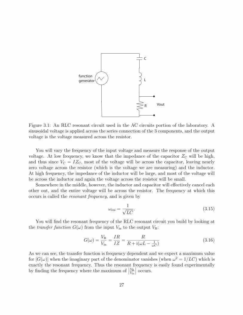
The circuit you will build to test these ideas (shown in Fig. 3.1) is called a series RLCresonant circuit, which is nothing more than an inductor, a capacitor, and a resistor con-nected in series. The series combination will be connected to a sinusoidal voltage source,and the voltage across the resistor will serve as the output voltage for your measurements.

1In this manual, i ≡√−1 is the imaginary unit. This can introduce some minor confusion with current,

which is also represented by the letter I (though always capitalized here), so it is not uncommon to see thesymbol j used to denote

√−1, particularly in the electrical engineering community. For Physics 4BL, we

will use i.

26

function

generator

R

L

C

Vout

Figure 3.1: An RLC resonant circuit used in the AC circuits portion of the laboratory. Asinusoidal voltage is applied across the series connection of the 3 components, and the outputvoltage is the voltage measured across the resistor.

You will vary the frequency of the input voltage and measure the response of the outputvoltage. At low frequency, we know that the impedance of the capacitor ZC will be high,and thus since VC = IZC, most of the voltage will be across the capacitor, leaving nearlyzero voltage across the resistor (which is the voltage we are measuring) and the inductor.At high frequency, the impedance of the inductor will be large, and most of the voltage willbe across the inductor and again the voltage across the resistor will be small.

Somewhere in the middle, however, the inductor and capacitor will effectively cancel eachother out, and the entire voltage will be across the resistor. The frequency at which thisoccurs is called the resonant frequency, and is given by

ωres =1√LC

. (3.15)

You will find the resonant frequency of the RLC resonant circuit you build by looking atthe transfer function G(ω) from the input Vin to the output VR:

G(ω) =VRVin

=IR

IZ=

R

R + i(ωL− 1ωC

)(3.16)

As we can see, the transfer function is frequency dependent and we expect a maximum valuefor |G(ω)| when the imaginary part of the denominator vanishes (when ω2 = 1/LC) which isexactly the resonant frequency. Thus the resonant frequency is easily found experimentallyby finding the frequency where the maximum of

∣∣∣ VRVin

∣∣∣ occurs.

27

3.2 Procedure and Measurement

3.2.1 RC Transient State Measurements

First, you will build an RC circuit with a resistor and capacitor in series and measure thevoltage on the capacitor during its charging. After that, you will build an RL circuit andmeasure the voltage on the inductor during the transient period. Instead of connectingthe circuit to a DC battery as described in the introductory section, we will use a squarewaveform produced by the function generator, which will repeatedly charge and dischargethe capacitor or inductor. You will measure the voltages with the DAQ connected to thecomputer and you will need to save the data to file to perform data analysis.

function

generator

R

C

Ch0+

Ch0-

Ch1+

Ch1-

Figure 3.2: An RC circuit connected to a function generator to measure the charging of thecapacitor as a function of time.

• Choose a resistor and capacitor combination giving a time constant τ = RC in a con-venient range to measure using the DAQ (≈ 10−3 seconds). Build a series connectioncircuit on top of the aluminum break-out box. The circuit you are building is shownin figure 3.2.

• Next, set the Rigol function generator to produce a square waveform with frequencyω < 1/τ . Set the amplitude of the waveform to be about 2 V, and use an offset equal tothe amplitude so that the waveform is at zero volts during the lower portion and ≈ 4 Vduring the upper portion of the square wave. A similar waveform to the one you wantto produce is shown in Fig. 3.3. Note that the Output button next to the BNC on theRigol function generator must be illuminated to produce output, which can be set bypushing the button once. Use the oscilloscope to verify that the function generator isproducing the desired square wave, then connect the signal to the aluminum break-outbox.

28

• Start the 4BL Application on the computer and set Acquisition Mode to Fixed Time.Using the Acquire module for two channels, use CH0 of the data acquisition system tomeasure the input waveform (the voltage drop across the series combination of R andC), and use CH1 to measure the voltage on the capacitor.

• Set the sample rate and the total points of measurement so that one or two full periodsare recorded and visible on the display. Observe how the voltage on the capacitorchanges when the input voltage jumps from zero volts to its peak voltage. Save thedata to a text file by pressing Save Waveform(s) to File.

−1 −0.8 −0.6 −0.4 −0.2 0 0.2 0.4 0.6 0.8 1

x 10−3

−1

0

1

2

3

4

5

6Square waveform with offset

time (seconds)

vo

lta

ge

(V

)

Figure 3.3: A square waveform is used as a impulse step-up voltage to study the transientof RC and RL circuits. The square wave is offset so that the lower voltage is at zero volts.

3.2.2 RL Transient State Measurements

Now we will measure the time constant of an RL circuit, using a large coil of copper wire asour inductor. This coil is part of a setup, shown in Figure 3.5, that will be used next week totest Faraday’s law of induction. To select the 1500 turn option, connect the driving currentinto the red port, and out of the black port labeled 1500.

For the RL circuit, it is important to note that the inductor has some internal resistanceof its own, which we will call Rint. We need to ensure that in building our RL circuit, theratio Rint/Rcircuit is small to minimize the effect the inductor’s internal resistance has on thewaveform. For the coil you’ll be using, Rint is on the order of 10s of ohms. To mitigate this,you simply need to make sure that you choose a larger resistor for the one that will be inseries with the inducting coil (maybe R ≈ 1 kΩ) to create our RL circuit.

With a BNC tee on the output of the function generator, send one output to the breakoutbox, and the other to Ch. 2 of the oscilloscope. Have the scope triggered on the rising edgeof the function generator signal on CH. 2.

Build the RL circuit shown in Figure 3.4 using the signal sent to the breakout box. Thedriving signal will be identical to the one used to investigate the RC circuit, but the frequency

29

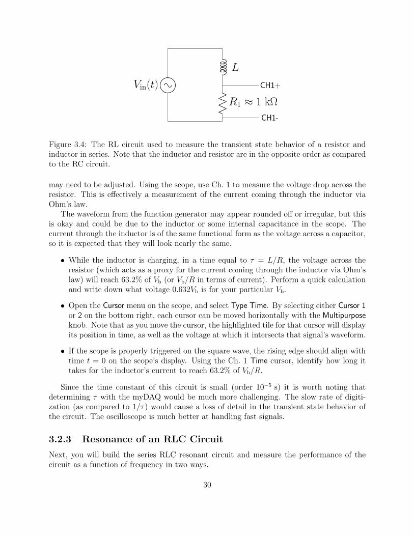
Figure 3.4: The RL circuit used to measure the transient state behavior of a resistor andinductor in series. Note that the inductor and resistor are in the opposite order as comparedto the RC circuit.

may need to be adjusted. Using the scope, use Ch. 1 to measure the voltage drop across theresistor. This is effectively a measurement of the current coming through the inductor viaOhm’s law.

The waveform from the function generator may appear rounded off or irregular, but thisis okay and could be due to the inductor or some internal capacitance in the scope. Thecurrent through the inductor is of the same functional form as the voltage across a capacitor,so it is expected that they will look nearly the same.

• While the inductor is charging, in a time equal to τ = L/R, the voltage across theresistor (which acts as a proxy for the current coming through the inductor via Ohm’slaw) will reach 63.2% of Vb (or Vb/R in terms of current). Perform a quick calculationand write down what voltage 0.632Vb is for your particular Vb.

• Open the Cursor menu on the scope, and select Type Time. By selecting either Cursor 1or 2 on the bottom right, each cursor can be moved horizontally with the Multipurposeknob. Note that as you move the cursor, the highlighted tile for that cursor will displayits position in time, as well as the voltage at which it intersects that signal’s waveform.

• If the scope is properly triggered on the square wave, the rising edge should align withtime t = 0 on the scope’s display. Using the Ch. 1 Time cursor, identify how long ittakes for the inductor’s current to reach 63.2% of Vb/R.

Since the time constant of this circuit is small (order 10−5 s) it is worth noting thatdetermining τ with the myDAQ would be much more challenging. The slow rate of digiti-zation (as compared to 1/τ) would cause a loss of detail in the transient state behavior ofthe circuit. The oscilloscope is much better at handling fast signals.

3.2.3 Resonance of an RLC Circuit

Next, you will build the series RLC resonant circuit and measure the performance of thecircuit as a function of frequency in two ways.

30

Figure 3.5: The inductor coil used for this experiment and Faraday’s law. Right: secondarycoil with option for 500, 1000, or 1500 turns. Left: A primary coil with 175 turns fits insidethe secondary coil, as does a magnetic core that boosts the inductance of the coils. Only thesecondary coil will be used for the RL circuit.

Method 1

First, you will identify the resonance by eye using a function generator and an oscilloscope.The circuit you will build is depicted in Fig. 3.1, where Vout will be measured on Ch. 1 ofthe oscilloscope. Choose a 1 µF capacitor, a 1 kΩ resistor, and use the secondary coil fromthe RL circuit (1500 turns).

To send Vin to the circuit, the breakout box will be needed. For measuring on the scope,we will have to convert the banana plug type connection to a BNC connection for the scope.There should be a BNC to banana plug converter to attach to the scope’s Ch. 1 input. It isrecommended that you build the RLC circuit with the secondary coil banana plug ports (i.e.put the resistor and capacitor directly onto the coil’s ports) to make this circuit portable formoving it to the myDAQ in Method 2. Connect the scope to measure the potential differenceacross the resistor (shown in Fig. 3.1 as Vout) using two wires going to the banana to BNCconverter on Ch. 1.

Before driving the circuit, first look at the function generator signal on Ch. 2 of the scope.We would like to set up the driving signal around resonance to minimize the time it takesidentify resonance. Use your value of τ from the RL circuit to estimate the inductance ofthe secondary coil at 1500 turns. Using your values of L and C, determine the theoreticalresonant frequency. Then, looking at the signal on the scope, ensure that you are applyinga sinusoidal signal at a frequency around resonance (within a few hundred Hz). Turn theamplitude of the signal all the way up on the function generator (with the offset set to zero),and use the measure function of the scope to determine the peak to peak amplitude of thesignal (twice the typical amplitude). We will be attempting to identify the frequency atwhich |Vout| is maximized and should equal the amplitude of the driving signal (implying a

31

gain |G| = 1).Feed the function generator’s BNC to the RLC side of the breakout box and set up

the scope to measure the amplitude of Vout. While adjusting the driving frequency on thefunction generator, observe the amplitude response of Vout and identify the frequency atwhich the amplitude of Vout is maximized. This is the resonant frequency. Take note ofpotential sources of error, and how they could affect your experimental value of ωres.

Method 2

Next, you will use the BODE Analyzer in the myDAQ 4BL software. A screen shot of theBODE software interface is shown in Fig. 3.7. This tool is located in the Instruments panel onthe Windows toolbar, which may be called something like NI ELVISmax Instrument launcher.Select the Bode Analyzer icon to start the software. The software’s purpose is to use themyDAQ to drive an AC current through a circuit and measure the voltage response as afunction of frequency. It graphs two quantities as a function of frequency, the magnitudeof the voltage response gain (

∣∣∣VoutVin

∣∣∣) and the phase response (which we will not use in this

experiment). The goal of this exercise is to find the resonant frequency for our circuit andto determine its quality factor, Q.

Figure 3.6: RLC circuit with values. Note the polarity of channels 0 and 1 of the myDAQare reversed with respect to each other. AO0 is the analog output channel 0 (white) andAGND is the analog ground (green) from the myDAQ.

• Connect the myDAQ channels as shown in Fig. 3.6. Connect the myDAQ’s whitewire (analog output, AO) to the capacitor side of the RLC circuit, and the green wire(ground, AGND) to the resistor side. Note that the power for the circuit comes fromthe white wire in and is then grounded with the green wire. Be careful to make sureyou are measuring the voltage properly over the correct elements with CH0 and CH1of the myDAQ.

• Using the Bode Analyzer software, adjust the options as you see fit in order to get agraph that will give you a good view of the resonance peak. This could possibly includethe Start/Stop Frequency, the number of Steps or the Peak Amplitude. The suggestedsettings are Mapping = Linear, Start Frequency = 20 Hz, Stop Frequency = 20 kHz, Steps(per decade) = 15.

32

Figure 3.7: Screen shot of the Bode Analyzer software showing the amplitude response (Gain,upper left) and phase response (Phase, lower left).

• Once you have a good looking graph that shows the resonant peak, estimate the reso-nant frequency. Save the data by using the Log button at the bottom right hand sideof the panel. Import these data into Excel to do your data analysis.2

3.3 Analysis

3.3.1 Transient Measurements

In the transient state measurements, you built and RC and an RL circuit and measured thevoltage across the reactive component during the transient period. By performing a linearregression after the data is linearized, you can determine the characteristic time scales of thetransient, τ = RC for an RC circuit. This analysis would be possible for the RL circuit aswell if we had used the myDAQ. You will be performing a linear regression for your RC datato determine the experimental value for τ = RC.

• Load the RC circuit data you obtained in §3.2.1 into Excel. Column A will probablybe time, column B is CH0 voltage which is the input square wave voltage, and columnC is the CH1 voltage (the voltage across the capacitor). The input square wave voltage

2If you have problems importing the data into proper columns, try using the Fixed width option and thenmoving the second break line a few characters to the right. If that doesn’t work, you may need to go throughyour data and delete some superfluous leading spaces and other characters that can make importing the datainto Excel difficult.

33

should always be near either zero volts or the peak voltage, which we can denote by Vb(note that the peak voltage likely occurs right before the falling edge of the waveformsince the RC circuit loads the function generator a little, causing it to deviate from itsideal value right after a rising edge). In your Excel file, find the row where the inputvoltage (column B) jumps from zero to Vb, and let’s call this row i. The input voltagewill stay at Vb for multiple rows until it drops back to zero. Find the last row wherethe voltage is at Vb and let’s call this row j. Copy the time (column A) data for rowsi through j to column D. Copy the CH1 voltages (column C) for rows i through j intocolumn E. Columns D and E now contain the time and capacitor voltage for only thetransient time period.

• Next, we are going to linearize the data since the voltage on the capacitor has anexponential dependence (Eq. 3.3). In column F, calculate (Vb−V (t))/Vb by subtractingthe data in column E by your value for Vband then dividing by that value. In columnG, calculate ln((Vb − V (t))/Vb) by taking the natural log of column F. Equation 3.3has now been linearized:

ln(Vb − V (t)

Vb

)= − t

RC(3.17)

• Perform a linear regression with time (column D) as your x-values, and the linearizeddata (column G) as your y-values. The magnitude of the slope given by the linearregression is 1/RC. Invert this number to determine τ and compare with the values Rand C you used in the circuit.

3.3.2 Resonant Circuit

The final task of your assignment was to build a resonant RLC circuit, and measure itsperformance as a function of frequency. To do this, you measured the peak-to-peak amplitudeof the output voltage at different frequencies. At the circuit’s resonant frequency, the outputvoltage was maximized. For analysis, you will compare your measured and theoretical valuesof fres ≡ ωres/2π obtained through the two separate methods, and calculate the quality factor,Q, which measures the sharpness of the resonance peak.

• Compare your measured values of fres (from both methods) with the theoretical value

fres =1

2π√LC

. Determine which method, 1 or 2, matches this theoretical value more

closely by finding the percent error for each from the theoretical value.

• Calculate the circuit’s Q-factor from method 2’s data, which measures the width ofthe resonance peak and the power loss in the circuit. To do so, first, plot your datain Excel (with a logarithmic x-axis) and find the voltage Vmax at f = fres. Thencalculate Vmax/

√2 and add a horizontal line to your plot at this voltage level3. This

3You can do this by, for instance, making two “data points” at appropriate places and plotting them asa scatter plot with a line connecting them.

34

line will intercept with your resonance curve at two points, with frequencies f1 and f2respectively. Estimate these frequencies and determine the Q-factor of the circuit:

Q =fres

f2 − f1. (3.18)

3.4 Lab Report

For this week’s experiment, the worksheet will be worth 40% and the presentation reportwill be worth 60% of your report grade.

3.4.1 Worksheet

Keeping a thorough record of what was observed in the laboratory is essential. Often, youwill need to refer back to your notes to confirm measured values and procedures to look forerrors.

1. In determining the resonant frequency of the RLC circuit, you used the BODE analyzersoftware to sample the gain of the circuit as a function of frequency. This relationship isof the form given in equation 3.16. The BODE software can sample frequencies rangingfrom 20 Hz to 20 kHz. Suppose that you obtain a resonance curve that never peakswithin this frequency range, but rather continues to increase all the way to 20 kHz.Since there is not a clear maximum value of the gain, the resonant frequency cannot bedetermined. Supposing your only goal is to observe a resonance on this plot and youare already using the largest L and C available to you, how could you alter the circuitto observe a resonance within the sampling range of the BODE software? (recall thatinductors add like resistors, and capacitors add opposite to resistors. Also assume theoriginal resonance was just out of range of the myDAQ, say 22 kHz).

2. Imagine you have two RLC circuits you are trying to scan for resonances using Method1. They have identical resonant frequencies, but circuit 1 has a very high Q-factor(Q1 1), and circuit 2 has a very low Q-factor (Q2 < 1). Lets assume you are alreadyon resonance and looking at Vout on the scope, and you change the frequency in eitherdirection for both circuits. How will the amplitude response differ between circuits 1and 2 as you move the driving frequency away from resonance?

3. This question is intended as in introduction to RLC resonant circuits.

Suppose the antenna in your car can pick any signal in the radio frequency spectrumwithout loss (fradio ∈ [3 kHz, 300 GHz]). Further suppose that if you were to look atVantenna on a scope, you would see a signal that is a superposition of all these frequencies.To mitigate this, we can send Vantenna through an RLC resonant circuit that has a verynarrow resonance curve (high Q-factor, ∆f very small). This causes all frequenciesother than a particular one at fres to attenuate, effectively tuning the radio to the

35

Figure 3.8: Diagram of a variable capacitor. The more the moving plates are rotated betweenthe fixed plates, the higher the capacitance

“fres” channel. In order to tune the radio to listen to a particular channel, the RLCcircuit has a variable capacitor in it whose capacitance changes as the radio tuningknob it turned.

What range of capacitance must the variable capacitor need to be tunable over tobe able to listen to the entire radio frequency spectrum, assuming the inductance inthe circuit is L = 1 mH? In reality, most of the RF spectrum is reserved for specificpurposes such as radiolocation, space research, the federal government, among otherthing. Now imagine now that the RLC circuit is composed of a single value capacitor(1 µF) and a variable inductor. What is the inductance range necessary to tune intojust the FM band? The FM radio band ranges from 88 MHz to 108 MHz.

4. A common use of capacitors as a reactive component is in a low-pass or high-pass filter,both of which contain a resistor and a capacitor. A low-pass filter is one that passesthrough signals with frequencies lower than a particular cutoff frequency and causesattenuation in signals of higher frequency. A high-pass filter is one that passes throughsignals with frequencies higher than a certain cutoff and causes lower frequencies toattenuate, giving the two configurations their names. The cutoff frequency for bothcircuits is given by ωc = (RC)−1.

In the interference lab later this quarter, a photometer will be used to convert lightintensity measurements to voltages in order to digitize a double slit interference pattern.This device takes incoming photons, and converts them into a voltage proportional tothe number of photons (which can be thought of as intensity). When using this device,the double slit pattern will be scanned very slowly, so that the voltage signal comingfrom the photometer changes slowly. Unfortunately, the photometer output has a lot

36

Figure 3.9: A low-pass filter (left) and a high-pass filter (right). Both Vin and Vout here aremeasured with reference to ground. That is, in measuring Vout with CH0 of the myDAQ,CHO+ would connect to Vout and CH0- would connect to ground.

of residual noise coming from the outlet it is plugged into (120 VAC, 60 Hz AC withnoise superimposed at much higher frequencies of order kHz or MHz). Given this,which type of filter should be used to filter the photometer output before allowing themyDAQ to measure the signal? Suggest a set of values of R and C, assuming that thesignal we care about has a frequency of about 3 Hz.

Additionally, suppose we have a noisy signal (superposition of many frequencies), butwe are only concerned with a particular part of the signal within the noise at a frequencyfdesired = 1 GHz. In a sentence or two, explain how you could isolate the desired partof the signal in the context of this problem. Assuming the noise is far from the desiredsignal in frequency (≥ ±200 MHz from fdesired), suggest component values that shouldachieve this effect.

3.4.2 Presentation Report

For the presentation report, you will be asked to present your data before and after manip-ulation, and explain important results. Additionally, you will write an introduction to thereport. The focus of the report should be the data and explaining its significance. Emphasison experimental design and procedure will come in later reports.

1. Cover Sheet (this will come before even the worksheet)

• Experiment number and title

• your name and UID

• the date the lab was performed

• your lab section (for instance, “Monday 2pm”)

37

• your TA’s name

• “Lab Partner(s):” followed by your lab partners’ names

2. Introduction

The introduction section explains, in your own words, the purpose of your experimentand how you will demonstrate this purpose. Try and be as brief as possible, yet stillget your point across.

3. Analysis

This section should present any calculations performed on the raw data, includinguncertainties using propagation of errors. For each required item, briefly explain thedata taken, present it in the most illuminating way possible, and analyze the resultsas succinctly as possible.

You should include:

• Graph of the linearized RC transient state data (V (t)). Explain the functionalform and results of linear regression. Identify your experimental value for τ = RC.

• Statement of measured L/R time, with a brief description as to how it was at-tained.

• Graph showing the output voltage (or gain) of the RLC resonant circuit as a func-tion of frequency from the BODE program. Explain the functional form. Comparethis resonant frequency with the one obtained by eye with the oscilloscope. In acouple sentences, explain which method you think is more accurate and why.

• Compare your experimental and theoretical values of the resonant frequency andcalculate the Q-factor of your resonant circuit.

38

Appendix A: Determining andReporting Measurement Uncertainties

Throughout this course, we will be making and reporting quantitative measurements ofexperimental parameters. In order to interpret the results of a measurement or experiment,it is crucial to specify the uncertainty (often called the “error” or “error bars”) with whichthe measurement claims to be a report of the “true value” of the quantity being measured.This chapter is designed to be a quick reference for the assignment and propagation of errorsfor your lab reports. For a more detailed treatment, I recommend the excellent books byTaylor [6] or Bevington and Robinson [1].

A.1 Statement of measured values in this course

Every measurement is subject to constraints that limit the precision and accuracy with whichthe measured “best value” corresponds to the “true value” of the quantity being measured.It is fairly standard in physics to use the following notation to specify both the measuredbest value and the uncertainty with which this value is known:

q = qbest ± δq. (A.1)

Here, q is the quantity for which we are reporting a measurement, qbest is the measuredbest value (often an average, but not infrequently generated in other ways) and δq is theuncertainty in the best value, which is defined to be positive and always has the same unitsas qbest. For our purposes in this course, the uncertainty will always be symmetric about themeasured best value, so the notation of Eq. A.1 will be used throughout.

For example, the most accurately measured quantities in the world are currently theratios of the energy splittings between pairs of special states in two atomic ions [5] and twoatoms [3], which are given by

νAl+

νHg+

= 1.052 871 833 148 990 44± 0.000 000 000 000 000 06 (A.2)

νYb

νSr= 1.207 507 039 343 337 75± 0.000 000 000 000 000 06 (A.3)

39

Focusing on the first value, the measured best value is 1.052 871 833 148 990 44 and the un-certainty is 6× 10−17. This level of precision and accuracy is far beyond anything we will bemeasuring in this course, but the notation in nonetheless understandable because it is givenin the form of Eq. A.1.

In this course, you will almost exclusively be measuring quantities with units. Measuredvalues for quantities that have units must be stated with their units. Failing to do so resultsin complete nonsense, the loss of $300 million space probes [4], dogs and cats living together,mass hysteria [2], not to mention the loss of points on your lab report grade. It is fine for theunits to appear as abbreviations, words, in column headers, after the numerical values, or insome combination of these just so long as it is clear what the units are. A good example ofhow to report a measured value is given by the 2010 CODATA recommended value for theproton mass:

mp = (1.672 621 78± 0.000 000 07)× 10−27 kg. (A.4)

Note that the parentheses are used around the measured best value and the uncertaintybecause they have the same units (which is always true) and are written with the sameexponential factor (which can help to make it easy to read).

There are two last points to make here about reporting measured values. First, in thesetwo examples, the uncertainties are written with the same precision (in scientific notation,the number of digits where we include any leading zeros) as the measured best value. Thisshould always be the case, and when you report a measured value with an uncertainty, youmust make sure the uncertainty is reported with the same precision as the measured bestvalue.

Second, if we disregard all of the leading zeros, the uncertainty is presented with onenonzero digit. There are times when it is appropriate to use up to two digits for this(particularly when the first digit of the uncertainty is small, say, a 1 or 2), but uncertaintiesshould never have three significant digits. This is because the size of the uncertainty itself setsthe scale of where the measurement can no longer claim to be providing useful information.

A.1.1 Other notation you will encounter

A quick glance at Eq. A.2 and A.4 reveals that it is difficult to read off the absolute value ofthe uncertainty, since one has to count a lot of zeros. For this course, you will be expected toreport your measurements in the form of Eq. A.1, but you should be aware of other methodsthat are used so that you can interpret their meaning.

Concise notation is useful when the fractional uncertainty becomes very small (as in theexamples above). In concise notation, only the significant digit or digits of the uncertainty arewritten, and they are written in parentheses directly after the best value, which is written tothe same precision. For example, the following shows two ways to express the same measuredvalue for the frequency of a laser

ν = (3.842 30± 0.000 02)× 1014 Hz (A.5)

ν = 3.842 30(2)× 1014 Hz. (A.6)

40

The second line uses concise notation, where since the number in parentheses has one digit,we are being told that this is the uncertainty in the last digit of the best value. This getsmore complicated when uncertainties are quoted with two digits, which seems to be gettingmore common in the literature. As a concrete example, the mass of the electron reportedby CODATA is actually reported in the following form:

me = 9.109 382 91(40)× 10−31 kg (A.7)

Here, we are being told that the last two digits have an uncertainty given by the two digitsin parentheses. This notation can seem somewhat confusing for a number of reasons, but ifwe always think of writing the digits in parentheses below the best value so that they endat the same place, it is easier to keep from getting confused, as in

me = 9.109 382 91× 10−31 kg

± 0.000 000 40× 10−31 kg (A.8)

Asymmetric uncertainties are also sometimes encountered in the scientific literature,where the upper uncertainty may have a different size than the lower one. In this case, thefollowing three examples show how one may see this written, using an example of a measuredradiative decay lifetime:

τ = (37.0 +2.0/−0.8) ms (A.9)

τ = (37.0 +2.0−0.8) ms (A.10)

τ = 3.70(+20−08)× 10−2 s (A.11)

A.1.2 “Sig Figs”

There is a system for implicitly including the order of magnitude of the uncertainty of ameasured quantity by simply stating the value with a certain number of digits, which isoften called the “sig figs” method for reporting uncertainty. Since our uncertainties will bedetermined with higher precision than their order of magnitude, we will not be using thisshorthand method in this course, and you will be expected to explicitly write the uncertaintyof your measured quantities, either in the form of Eq. A.1 or as a separate column entryin a table. However, you should be aware of this shorthand since it does get used, thoughtypically outside of formal scientific literature.

Aside from its lack of specificity, an additional drawback of the sig figs method for report-ing uncertainties is that all too often it leads to laziness and people reporting numbers withimplicit uncertainties far better than are actually merited. Your author starts to becomesuspicious that this might be happening when measurements of continuous quantities arereported to 4 or more digits, particularly by non-scientists. At or after the 4th digit, onehas to think seriously about things such as the calibration and resolution of measurementequipment, thermal expansion of tape measures and rulers, finite response time and jitter oftiming systems, the linearly and stability of spring constants, surface roughness and cleanli-ness, not to mention whether it makes sense at all to define the quantity you’re measuringto that scale.

41

Example A.1 Your author just looked at espn.com and noticed that they report thespeeds of NASCAR racers to 6 digits. They claim that, for instance, Kyle Busch justcompleted a lap with an average speed of 126.648 mph. Can you think of reasonsto suspect that some (perhaps half) of these digits should not be believed? Hint:was the length of the track even known to 6 digits at that particular time on thatparticular day [8]?

A.1.3 Accuracy and Precision

In physics and other sciences, the words accuracy and precision mean different things, andit is important to distinguish between them. The accuracy of a measurement is how closethe measured value is to the true value of the quantity being measured. If the true value iswithin the uncertainty that is reported, we find that the measurement was accurate.

Estimating the accuracy of a measurement is notoriously difficult without knowing thetrue value. The standards that must be met to produce quantitative accuracy estimates varyfrom field to field, but they generally consist of trying to estimate the size of the impact ofevery possible source of error.

One cheap way to make a measurement that won’t be inaccurate is to construct themeasurement poorly on purpose so that the uncertainty is gigantic and is thereby highlylikely to overlap with the true value. However, this illustrates the point that accuracy is notvery useful without another key ingredient of a good measurement: precision.

The precision of a measurement is how small the range is that a statistical spread ofrepeated measurements will fall into. The precision tells us nothing about the accuracy ofa measurement, and is determined entirely without knowing the true value of the quantitybeing measured. Measurement precision is often determined by the statistical spread ofrepeated measurements, and it will be fairly standard in this course to use the standarddeviation of a collection of repeated measurements to set the precision of the reported mea-sured value (see § A.1.6 for a more sophisticated treatment). However, the resolution of themeasurement tool itself could be larger than this spread, in which case the quoted precisionwill be dominated by the instrument resolution.

Exercise A.1 A researcher needs to determine the diameter of a 10 cm long quartzrod to make sure it will fit the mirror mounts for an optical cavity. The calipersused have a digital display whose most-precise digit is in the 0.01 mm place. 10measurements along the length of the rod all yield the same reading on the display,5.98 mm. It is clear that the measured best value is dbest = 5.98 mm, but how canthe uncertainty δd of the measurement be determined?

A.1.4 Computer use and too many digits

A common mistake that students make in reporting measured values is to have too many(way too many) digits on their numbers. After all, the computer will report a measured valueoften to 16-bit precision, which gives a relative precision of 10−5. However, just because a

42

computer gives you a number with 5 digits of precision does not mean that the measurementis accurate at that level. If you have a computer multiply a raw measured value of somethingby π, for instance, the computer will happily tell you the answer to 50 digits. This may lookimpressive at first, but if the original number is only measured to 2 digits, all of that extrastuff is nonsense.

For example, if you see that repeated measurements of the same quantity fluctuate atabout the 3rd decimal place, there is not going to be much useful information in the 8thdecimal place and it should probably not find its way into your report in any form. In thiscase, it would make sense to hang on to maybe 4 or 5 digits during the calculations and formaking tables of your raw data. However, the uncertainty is likely to be in the 3rd digit inthe end, in which case you will be throwing out everything after the 3rd digit in your finalreported number and there is no reason to keep hauling those 8th digits around, clutteringup your spreadsheets and implying an unrealistic uncertainty in your numbers. If you keepthings simple, you will find that the physics is easier to see!

A.1.5 Sources of uncertainty

There are many factors that can contribute to uncertainty in measured quantities. Thesesources are often separated into two types, systematic uncertainty and statistical uncertainty.This is a slight oversimplification, but for our purposes in this course, sources of statisticaluncertainty tend to produce a random distribution of data points about the mean uponrepeated measurements of the same quantity. As such, statistical uncertainty affects theprecision of measured values, but not the accuracy.

Systematic uncertainty, on the other hand, affects all of the measured data points in thesame way and therefore does not contribute to the statistical spread. Systematic uncertaintylimits the accuracy of a measurement, but not the precision of the measured value. If youneed to compare your measured value to a known true value (for instance, perhaps in ameasurement of the charge of the electron, e), you will need to consider systematic effects,particularly if you find that your measurement was inaccurate (the true value does not fallwithin your uncertainty of your measured best value).

However, we will primarily be concerned with quantitative assessments of statistical un-certainty in this course. To reiterate an earlier point, you are likely to encounter two maintypes of statistical uncertainty in this course, those due to finite instrument resolution andthose due to “noise” sources that cause repeated measurements of the same quantity to fluc-tuate. The quantitative method for combining multiple sources of uncorrelated uncertaintiesis covered in section A.2.

A.1.6 Estimation of Statistical Uncertainty in a Mean

One way to estimate the statistical uncertainty in a measurement is to repeat the mea-surement many times and to look at the spread in measured points. This method is onlyapplicable in cases where the precision is limited by statistics (instead of, for instance, in-strument resolution), but will be commonly encountered and so we provide a summary of

43

the procedure here.Let us assume we have a set of N data points xi that all measure some quantity x. If

we do not have a good estimate for the uncertainty in each xi, we can still combine them tocome up with a best value and uncertainty in x by looking at their statistics.

For our purposes in this course, we may assume xbest = x, which is to say that the bestvalue for our measurement of x is the mean of our measured points

x =1

N

N∑i=1

xi. (A.12)

One commonly used method for estimating the uncertainty in our knowledge of x is touse the standard deviation (σx) of the collection of points xi. The standard deviation is ameasure of the spread of points around a mean value. In our case, we should use the so-calledsample standard deviation1, given by

σx ≡

√√√√ 1

N − 1

N∑i=1

(xi − x)2. (A.13)

The reason we divide by N − 1 instead of N is that x was determined from the datapoints themselves and not independently. In Microsoft Excel, the functions STDEV() andSTDEV.S() both calculate the sample standard deviation using the formula above and youmay use either one if you don’t want to enter that formula manually.

While it is probably okay in most cases in this course to use the sample standard deviationas an estimate of the statistical uncertainty in the mean, there is something about this thatis missing. Specifically, the problem with using δx = σx is that it does not really get smalleras you collect more data. However, if we take 100 times as many data points as we had andthey have the same spread as our original data set, we should be able to use this to comeup with a significantly better measurement of x since we get to average over 100 times asmany individual data points. Specifically, we should get a statistical uncertainty that is 10times smaller if we take 100 times as many data points, which fact is evident when we usethe following formula to calculate our statistical uncertainty:

δx =σx√N

=1√N

√√√√ 1

N − 1

N∑i=1

(xi − x)2. (A.14)

You may apply Eq. A.14 anytime you are trying to estimate the statistical uncertainty inthe mean of a collection of data points based only on the distribution of those points.

A.1.7 Summary

When writing your lab report, you may at times be asked by your TA to include raw data inyour report. This will likely take the form of a table of some kind. Raw data does not need

1There is also something called a population standard deviation, which differs from Eq. A.13 in that thefactor of 1/(N − 1) is replaced by 1/N . The population standard deviation is appropriate in cases where themean of the parent distribution is determined independently from the data.

44

to have explicit uncertainties for each entry unless you are specifically asked to provide it.However, even your raw data must have units labeled. This can be done in column headersor plot axis labels, but there should not be any room for ambiguity on this point.

• Every single number in your report that describes a quantity that has units must haveits units clearly labeled in your report.

When reporting the results of measurements in your report (as opposed to just showingexamples of raw data), you will be expected to report the measured best value and theuncertainty. When you quote the final measured value of a quantity in your report, be surethat

• You report the measured best value and the uncertainty: q = qbest ± δq

• You include proper units

• The measured best value and the uncertainty are written with the same absoluteprecision

• The uncertainty has no more than two significant digits

A.2 Propagation of uncertainties

Fairly often in the laboratory we will be measuring many different quantities and combiningthose measurements together in some mathematical way to come up with a measured valuefor a composite quantity. For instance, let’s say we wanted to measure the effective resistanceof an electronics complnent by using two multimeters to measure the current I through thedevice when a voltage V is applied across it. Using the guidelines above, we will haveassigned an uncertainty to each of these quantities, so we want to know how to turn ourmeasured values for the parameters Vbest ± δV and Ibest ± δI into a measured value for thecomposite quantity, the resistance R = Rbest ± δR.

The way we do this is by using the functional form of how the composite quantitydepends upon the input parameters to mathematically determine the resulting uncertaintyin the composite quantity. It is important to use the following methods only in the caseswhere the uncertainties are uncorrelated, so be sure that the uncertainties are generated byphysically independent mechanisms (statistical uncertainties typically fall firmly into thiscategory).

We will write the expression relating the uncertainty δf of some composite quantity f tothe uncertainties (δx, · · · , δz) of the parameters used to compute f = f(x, · · · , z) withoutproof or derivation (see, e.g., [1]):

δf =

√√√√(∂f∂x

δx

)2

+ · · ·+(∂f

∂zδz

)2 ∣∣∣∣∣xbest,···,zbest

(A.15)

45

where the vertical line on the right side instructs us to evaluate the resulting expression atx = xbest, · · · , z = zbest.

2

If you are not familiar with the notation of those derivatives (∂f/∂x), they are calledpartial derivatives and simply instruct you to treat everything except the variable of differ-entiation as a constant when taking the derivative. If we come back to our example of themeasurement of the resistance of an electronics component, we first identify f = R = V/I.We need to determine δR in terms of Vbest, δV , Ibest, and δI. We can begin by taking thepartial derivatives:

∂R

∂V=

∂

∂V

(V

I

)=

1

I(A.16)

and∂R

∂I=

∂

∂I

(V

I

)= −V

I2. (A.17)

This gives us

δR =

√(1

IδV)2

+(−VI2δI)2∣∣∣∣∣Vbest,Ibest

=1√I2

√(δV )2 +

V 2

I2(δI)2

∣∣∣∣∣Vbest,Ibest

=

√V 2

I2

√√√√(δVV

)2

+

(δI

I

)2 ∣∣∣∣∣Vbest,Ibest

. (A.18)

Normally, we would say that√V 2/I2 = ±V/I to reflect the two solutions of that equation.

However, we have defined all uncertainties (δq in Eq. A.1) to be positive, so here we takethe absolute value: ∣∣∣∣∣∣

√V 2

I2

∣∣∣∣∣∣ =∣∣∣∣VI∣∣∣∣ . (A.19)

We can now evaluate our expression at V = Vbest and I = Ibest to give us

δR =∣∣∣∣VbestIbest

∣∣∣∣√√√√( δV

Vbest

)2

+

(δI

Ibest

)2

. (A.20)

We have identified Rbest = Vbest/Ibest, so dividing both sides by the absolute value of thisquantity and noting that we can add an absolute value sign to both terms under the radicalsince they are squared anyway gives us the following symmetric-looking form:

δR

|Rbest|=

√√√√( δV

|Vbest|

)2

+

(δI

|Ibest|

)2

. (A.21)

2The assumption we are going to invoke here is that fbest = f(xbest, · · · , zbest). This is sometimes notstrictly correct, but will serve for the purposes of this course.

46

The quantity δq/|qbest| is called the fractional uncertainty or relative uncertainty of somemeasurement of q, so we can restate Eq. A.21 in words by saying that the fractional uncer-tainty in a ratio of two quantities is given by the quadrature sum of the fractional uncer-tainties of the two quantities.

A.2.1 Specific formulas

While the form given in Eq. A.15 is sufficiently general to allow it to be applied directly forevery case encountered in this course, we can summarize some of the most common resultsthat can be derived from it as follows.

• Measured quantity (x) times an exact number (A): f = Ax

δf = |A| δx (A.22)

• Sums and differences (they follow the same rule): f = x+ y − z + · · ·

δf =√

(δx)2 + (δy)2 + (δz)2 + · · · (A.23)

• Products and ratios (they follow the same rule): f = x×···×zu×···×w

δf

|fbest|=

√√√√( δx

|xbest|

)2

+ · · ·+(

δz

|zbest|

)2

+

(δu

|ubest|

)2

+ · · ·+(

δw

|wbest|

)2

(A.24)

• Measured quantity raised to an exact number power (n): f = Axn

δf

|fbest|= |n| δx

|x|(A.25)

• Exponential with measured quantity in the exponent f = Aeax

δf

|fbest|= |a| δx (A.26)

You may recognize that Eq. A.21 is a special case of Eq. A.24, as is Eq. A.22. And, ofcourse, all of these are special cases of Eq. A.15. These cases are not the only possibilitiesfor functional forms of the relationships between measured values, but they are the mostcommon for us in this course. You should be sure to keep in mind that these formulas arevalid only for uncertainties that are uncorrelated.

47

Appendix B: Linear Regression inExcel

A Linear regression is done by the either “least squares” or minimum Chi Squared method.Suppose you have some set of data that you have plotted against each other, x and y, and youwant to run a regression line through it. You write the equation of a line: y = m[x]+b. In thiscase you can have at most two parameters that you can vary to completely describe the line.These parameters are m and b. When a linear regression is performed, the parameters areset usually randomly and the sum of the square of the residuals is computed. The residualsare the difference between your data point y, and what you expect to calculate from yourregression line at that x value so m[x] + b. You do that for every data point then squarethem and you have the sum of the residuals squared. The program will then change theparameters m and b and calculate the sum of the residuals squared repeatedly over a certainrange of values. It will then take the parameters m and b that correspond to the minimumvalue of the sum of the residuals squared, and take that for the slope of the final regressionline. Notice that this method neglects the uncertainties (error bars) on each point.

To make the least squares regression line appear on the plot, right click on any data pointthen select Add trendline. Highlight linear and click on the options tab. Here you can selectwhether or not to set the Intercept to zero, which will be discussed in more detail later whenI talk about all of the regression data. Click ok to add the line.

• Make sure that you have an internet connection and add the Analysis package to Excel.You can do this by going to the menu and clicking tools then Add-ins. Next check thebox next to Analysis toolpack and hit ok. Follow the instructions and the package willbe installed.

• We can now use the analysis package. After you have made your plot for your analysis,make sure that you click an empty cell, go to Tools, Data Analysis. This will opena window with several analysis functions you can use. Scroll down until you findRegression. Highlight it by clicking it and hit ok.

• This will open a new window. In the Input Y Range, drag a box around your y datavalues. In the Input X range, drag a box around your x data values. You need tomake a decision as to whether or not you want the constant to be fixed at zero. For

48

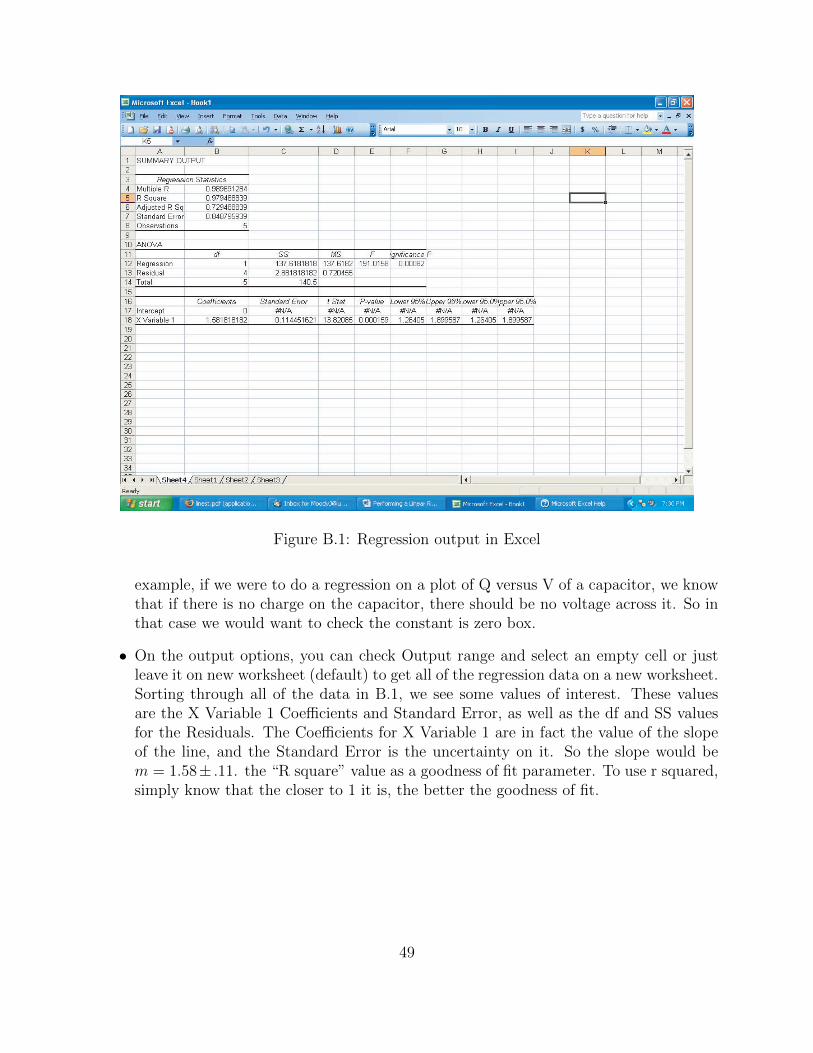
Figure B.1: Regression output in Excel

example, if we were to do a regression on a plot of Q versus V of a capacitor, we knowthat if there is no charge on the capacitor, there should be no voltage across it. So inthat case we would want to check the constant is zero box.

• On the output options, you can check Output range and select an empty cell or justleave it on new worksheet (default) to get all of the regression data on a new worksheet.Sorting through all of the data in B.1, we see some values of interest. These valuesare the X Variable 1 Coefficients and Standard Error, as well as the df and SS valuesfor the Residuals. The Coefficients for X Variable 1 are in fact the value of the slopeof the line, and the Standard Error is the uncertainty on it. So the slope would bem = 1.58± .11. the “R square” value as a goodness of fit parameter. To use r squared,simply know that the closer to 1 it is, the better the goodness of fit.

49

Appendix C: Data Acquisition

A desktop computer is provided on each station. The operating system is some flavor ofWindows. Available software includes Microsoft Office and custom-written modules basedon National Instruments LabVIEW. A limited internet connection is provided so that youcan access webmail for emailing data. Alternatively, you may use a USB flash drive fortransporting your data.

C.1 DAQ

A data acquisition card from National Instruments (NI6024E) is installed in the computer. Itcontains a 12 bit, 200 ksample/sec Analog to Digital Convertor (ADC). Up to 8 differentialinput signals can be measured. Multiplexing between several input signals decreases theconversion speed. The maximum input voltage range is ±10 V. The common-mode voltage(voltage of each channel to ground) is also limited to 10 V.

C.1.1 Input

The inputs for the ADC are at a connector box. The BNC coax connector on the left sideof the front panel is the input for an external trigger signal (TTL, ±5 V). To provide thetrigger signal, connect the TTL output on the signal generator and this trigger signal inputwith a BNC cable.

Three input channels (±10 V maximum) are marked on the front panel as three pairs of+ and −. From left to right, we name them Channel 1, 2, and 3. The inputs are differential,i.e., neither electrode is connected to ground, and what the computer measures is the voltagedifference between + and − terminals at each channel. Connections are made by alligatorclips.

C.1.2 Software

The data acquisition is controlled by LabVIEW Virtual Instruments modules. The modulesare accessed via a software, called ”4BL Main Menu”, whose shortcut icon is on the screen.If it has been removed, the full path is C:\Program Files\4BL\Main Menu. Once we open

50

the software by double-clicking the icon, a main menu for this data acquisition software willbe displayed. We can then further choose different functions to perform according to thetask we would like to complete. The following two functions will be frequently used in thiscourse.

Acquire waveforms

This program is used to measure voltages at one or more channels as a function of time forrepetitive waveforms. In order to synchronize the data acquisition a trigger input is required.The program works like a digital oscilloscope.

To start acquiring waveform on only one channel (Channel 1), single-click “Acquire Wave-form (1 Channel)” on the main menu. There are a couple of parameters we should specify.

1. Set the expected limits of the measured voltages. Voltages higher than the limit willbe truncated in the measurement.

2. Choose the scan rate, i.e., how many samples are acquired within a second.

3. Set the total number of points to acquire.

4. Choose the time limit for acquiring data.

First, we should When every setting is ready, click “Acquire” and you will see the waveformon Channel 1 displayed as a function of time. The time span is given by the ratio of thenumber of points acquired and the number of points per second. The default displayedvoltage range (5 V) can be changed by highlighting the upper or lower voltage limit, typingin the desired value followed by “Enter”. When satisfied, single-click “Save to file”. Itprompts for a file name (e.g., Oct29-2.xls) to be saved. To get out of the data acquisitionprogram, click on “Stop?”, “Done”.

If we would like to sample two channel waveforms simultaneously, single-click “AcquireWaveforms (2 Channel)” on the main menu. This will enable us to sample the waveforms onboth Channel 1 and 2. The sampling procedure is the same as in sampling only one channel.Signals on different channels are identified by the displayed curve colors.

After acquired the waveforms on two channels, we could also study the statistical prop-erties of the two channels by single clicking the ”Statistics”. A new window will pop up,showing the mean value and standard deviation for both channels, and the covariance, cor-relation between channels as well.

Sample signals continuously

This program is used to record a slowly varying signal. It records data at specified timeintervals, writes continuously to file until stopped by terminating the program. No triggeris required. The program is also called a ”data logger”.

To call the program double-click ”4BL Main Menu”, single click ”Sample 1 channel(continuously)” which prompts for various parameter choices:

51

1. Single-click on ”Reset limits” and adjust high and low values in units of 1 V or fractionsthereof by typing over the displayed numbers. Press ”Done” to exit.

2. Single-click on ”Time between points” and increment in units of 1 sec or fractionsthereof by typing over the displayed numbers.

3. Single-click on ”Acquire” and specify a file name (e.g., Oct29-3.xls). When you press”Save” the program starts to record.

The waveform is displayed on a screen with 64 horizontal data points. It will scroll in time.The vertical scale changes automatically to display the signal at any amplitude. However,it saturates when the specified voltage limits are exceeded. When satisfied single-click on”Stop acquiring” to end the data file. If you want to take another file press ”Acquire” again.You can overwrite (replace) an existing file but you cannot append to a file. If you want toget out of the program to process the file, press ”Done?” to quit.

We could also sample more than one channel signals continuously by choosing ”Sample 2channel (continuously)”, for example for 2 channels. The procedure is the same as describedabove.

52

Appendix D: DC Power Supply

D.1 Description

The power supply in each station is able to provide a constant DC voltage during theexperiments, see Fig. D.1. There are three terminals on the right hand side of the frontpanel. The voltage output can be obtained from the red + and the black - terminals, whilethe green one in the middle is grounded at all times.

Figure D.1: A photo of the power supply.

D.1.1 On and Off

The main control knob locates at the center of the front panel. To turn on the power supply,simply turn this knob clockwise. After a click sound a green light named POWER abovethis knob will be turned on, indicating the power supply is working properly. When theexperiment is finished, please remember to power off the supply by turning this knob all theway counterclockwise until a click sound.

53

There is also a switch on the top of the front panel. The switch could be on either STBYor DC ON positions. During the experiments, if you would like to power off the supplytemporarily, you could simply put the switch on STBY position.

D.1.2 Adjust Voltage

The output voltage could be adjusted by turning the main knob mentioned above. Theoutput voltage range, either 0 − 50 V or 0 − 25 V, is set by a switch next to the knob.There is also a voltmeter on the right side of the front panel, which enables us to monitorthe output voltage.

D.1.3 Overload

The power supply can afford only a certain amount of current flowing through it. Themaximum amount of current can be set by another knob on the left side of the front panel,and the current level can be monitored from the amperemeter next to this knob.

If the current is above the maximum current we set, the power supply will automaticallyshut down, and a red OVERLOAD light next to the amperemeter will be turned on at thesame time. In this case, you should reduce the current to the correct range, and press thered RESET button on the upper left corner of the front panel to reset the power supply.

54

Bibliography

[1] Philip R. Bevington and D. Kieth Robinson. Data Reduction and Error Analysis for thePhysical Sciences. McGraw-Hill, Inc., 2nd edition, 1992.

[2] William J. Murray, 1984.

[3] Nils Nemitz, Takuya Ohkubo, Masao Takamoto, Ichiro Ushijima, Manoj Das, NoriakiOhmae, and Hidetoshi Katori. Frequency ratio of Yb and Sr clocks with 5 × 10−17

uncertainty at 150 seconds averaging time. Nature Photonics, 10:258, 2016.

[4] Tony Reichhardt. NASA reworks its sums after Mars fiasco. Nature, 401:517, 1999.

[5] T. Rosenband, D. B. Hume, P. O. Schmidt, C. W. Chou, A. Brusch, L. Lorini, W. H.Oskay, R. E. Drullinger, T. M. Fortier, J. E. Stalnaker, S. A. Diddams, W. C. Swann,N. R. Newbury, W. M. Itano, D. J. Wineland, and J. C. Bergquist. Frequency ratio ofAl+ and Hg+ single-ion optical clocks; metrology at the 17th decimal place. Science,319:1808, 2008.

[6] John R. Taylor. An Introduction to Error Analysis. University Science Books, Sausalito,California, 2nd edition, 1997.

[7] J. J. Thomson. Cathode rays. Philosophical Magazine, 44(269):293, 1897.

[8] Menglan Zeng and Donald H. Shields. Nonlinear thermal expansion and contraction ofasphalt concrete. Can. J. Civ. Eng., 26:26, 1999.

55