physics 6b lab manual - uclademoweb.physics.ucla.edu/sites/default/files/physics6b_manual_0.pdf ·...
TRANSCRIPT
Physics 6B Lab ManualUCLA Physics and Astronomy Department
Primary authors: Art Huffman, Ray Waung
1
Physics 6B LabIntroduction
PURPOSE
The laws of physics are based on experimental and observational facts. Laboratory work is thereforean important part of a course in general physics, helping you develop skill in fundamental scientificmeasurements and increasing your understanding of the physical concepts. It is profitable for you toexperience the difficulties of making quantitative measurements in the real world and to learn howto record and process experimental data. For these reasons, successful completion of laboratorywork is required of every student.
PREPARATION
Read the assigned experiment in the manual before coming to the laboratory. Since each experimentmust be finished during the lab session, familiarity with the underlying theory and procedure willprove helpful in speeding up your work. Although you may leave when the required work iscomplete, there are often “additional credit” assignments at the end of each write-up. The mostcommon reason for not finishing the additional credit portion is failure to read the manual beforecoming to lab. We dislike testing you, but if your TA suspects that you have not read the manualahead of time, he or she may ask you a few simple questions about the experiment. If you cannotanswer satisfactorily, you may lose mills (see below).
RESPONSIBILITY AND SAFETY
Laboratories are equipped at great expense. You must therefore exercise care in the use of equip-ment. Each experiment in the lab manual lists the apparatus required. At the beginning of eachlaboratory period check that you have everything and that it is in good condition. Thereafter, youare responsible for all damaged and missing articles. At the end of each period put your placein order and check the apparatus. By following this procedure you will relieve yourself of anyblame for the misdeeds of other students, and you will aid the instructor materially in keeping thelaboratory in order.
The laboratory benches are only for material necessary for work. Food, clothing, and other personalbelongings not immediately needed should be placed elsewhere. A cluttered, messy laboratorybench invites accidents. Most accidents can be prevented by care and foresight. If an accident doesoccur, or if someone is injured, the accident should be reported immediately. Clean up any brokenglass or spilled fluids.
FREEDOM
You are allowed some freedom in this laboratory to arrange your work according to your own taste.The only requirement is that you complete each experiment and report the results clearly in yourlab manual. We have supplied detailed instructions to help you finish the experiments, especially
2
Physics 6B Lab
the first few. However, if you know a better way of performing the lab (and in particular, a differentway of arranging your calculations or graphing), feel free to improvise. Ask your TA if you are indoubt.
LAB GRADE
Each experiment is designed to be completed within the laboratory session. Your TA will check offyour lab manual and computer screen at the end of the session. There are no reports to submit.The lab grade accounts for approximately 15% of your course total. Basically, 12 points (12%) areawarded for satisfactorily completing the assignments, filling in your lab manual, and/or displayingthe computer screen with the completed work. Thus, we expect every student who attends alllabs and follows instructions to receive these 12 points. If the TA finds your work on a particularexperiment unsatisfactory or incomplete, he or she will inform you. You will then have the optionof redoing the experiment or completing it to your TA’s satisfaction. In general, if you work on thelab diligently during the allocated two hours, you will receive full credit even if you do not finishthe experiment.
Another two points (2%) will be divided into tenths of a point, called “mills” (1 point = 10 mills).For most labs, you will have an opportunity to earn several mills by answering questions related tothe experiment, displaying computer skills, reporting or printing results clearly in your lab manual,or performing some “additional credit” work. When you have earned 20 mills, two more pointswill be added to your lab grade. Please note that these 20 mills are additional credit, not “extracredit”. Not all students may be able to finish the additional credit portion of the experiment.
The one final point (1%), divided into ten mills, will be awarded at the discretion of your TA. Heor she may award you 0 to 10 mills at the end of the course for special ingenuity or truly superiorwork. We expect these “TA mills” to be given to only a few students in any section. (Occasionally,the “TA mills” are used by the course instructor to balance grading differences among TAs.)
If you miss an experiment without excuse, you will lose two of the 15 points. (See below for thepolicy on missing labs.) Be sure to check with your TA about making up the computer skills; youmay be responsible for them in a later lab. Most of the first 12 points of your lab grade is basedon work reported in your manual, which you must therefore bring to each session. Your TA maymake surprise checks of your manual periodically during the quarter and award mills for complete,easy-to-read results. If you forget to bring your manual, then record the experimental data onseparate sheets of paper, and copy them into the manual later. However, if the TA finds that yourmanual is incomplete, you will lose mills.
In summary:
3
Physics 6B Lab
Lab grade = (12.0 points)
− (2.0 points each for any missing labs)
+ (up to 2.0 points earned in mills of “additional credit”)
+ (up to 1.0 point earned in “TA mills”)
Maximum score = 15.0 points
Typically, most students receive a lab grade between 13.5 and 14.5 points, with the few pooreststudents (who attend every lab) getting grades in the 12s and the few best students getting gradesin the high 14s or 15.0. There may be a couple of students who miss one or two labs without excuseand receive grades lower than 12.0.
How the lab score is used in determining a student’s final course grade is at the discretion of theindividual instructor. However, very roughly, for many instructors a lab score of 12.0 representsapproximately B− work, and a score of 15.0 is A+ work, with 14.0 around the B+/A− borderline.
POLICY ON MISSING EXPERIMENTS
1. In the Physics 6 series, each experiment is worth two points (out of 15 maximum points). Ifyou miss an experiment without excuse, you will lose these two points.
2. The equipment for each experiment is set up only during the assigned week; you cannotcomplete an experiment later in the quarter. You may make up no more than one experimentper quarter by attending another section during the same week and receiving permission fromthe TA of the substitute section. If the TA agrees to let you complete the experiment in thatsection, have him or her sign off your lab work at the end of the section and record your score.Show this signature/note to your own TA.
3. (At your option) If you miss a lab but subsequently obtain the data from a partner whoperformed the experiment, and if you complete your own analysis with that data, then youwill receive one of the two points. This option may be used only once per quarter.
4. A written, verifiable medical, athletic, or religious excuse may be used for only one experimentper quarter. Your other lab scores will be averaged without penalty, but you will lose anymills that might have been earned for the missed lab.
5. If you miss three or more lab sessions during the quarter for any reason, your course grade willbe Incomplete, and you will need to make up these experiments in another quarter. (Notethat certain experiments occupy two sessions. If you miss any three sessions, you get anIncomplete.)
4
Physics 6B Lab | Experiment 1
Driven Harmonic Oscillator
APPARATUS
• Computer and interface
• Mechanical vibrator and spring holder
• Stands, etc. to hold vibrator
• Motion sensor
• C-209 spring
• Weight holder and five 100-g mass disks
INTRODUCTION
This is an experiment in which you will plot the resonance curve of a driven harmonic oscillator.Harmonic oscillation was covered in Physics 6A, so we include a partial review of both the underlyingphysics and the Pasco Data Studio. We will continue to give fairly detailed instructions for takingdata in this first Physics 6B lab. However, this is the last experiment with detailed instructions onsetting up Data Studio. Henceforth, it will be assumed that you know how to connect the cablesto the computer and to the sensors; how to call up a particular sensor; and how to set up a table,graph, or digit window for data taking.
THEORY
Hooke’s Law for a mass attached to a spring states that F = −kx, where x is the displacementof the mass from equilibrium, F is the restoring force exerted by the spring on the mass, and k isthe (positive) spring constant. If this force causes the mass m to accelerate, then the equation ofmotion for the mass is
−kx = ma. (1)
Substituting for the acceleration a = d2x/dt2, we can rewrite Eq. 1 as
−kx = md2x/dt2 (2)
or
d2x/dt2 + ω20x = 0, (3)
where ω0 =√k/m is called the resonance angular frequency of oscillation. Eq. 3 is the differential
equation for a simple harmonic oscillator with no friction. Its solution includes the sine and cosinefunctions, since the second derivatives of these functions are proportional to the negatives of thefunctions. Thus, the solution x(t) = A sin(ω0t) +B cos(ω0t) satisfies Eq. 3. The parameters A andB are two constants which can be determined by the initial conditions of the motion. The naturalfrequency f0 of such an oscillator is
f0 = ω0/2π = (1/2π)√k/m. (4)
5
Physics 6B Lab | Experiment 1
In the simple case described above, the oscillations continue indefinitely. We know, however, thatthe oscillations of a real mass on a spring eventually decay because of friction. Such behavioris called damped harmonic motion. To describe it mathematically, we assume that the frictionalforce is proportional to the velocity of the mass (which is approximately true with air friction, forexample) and add a damping term, −b dx/dt, to the left side of Eq. 2. Our equation for the dampedharmonic oscillator becomes
−kx− b dx/dt = md2x/dt2 (5)
or
md2x/dt2 + b dx/dt+ kx = 0. (6)
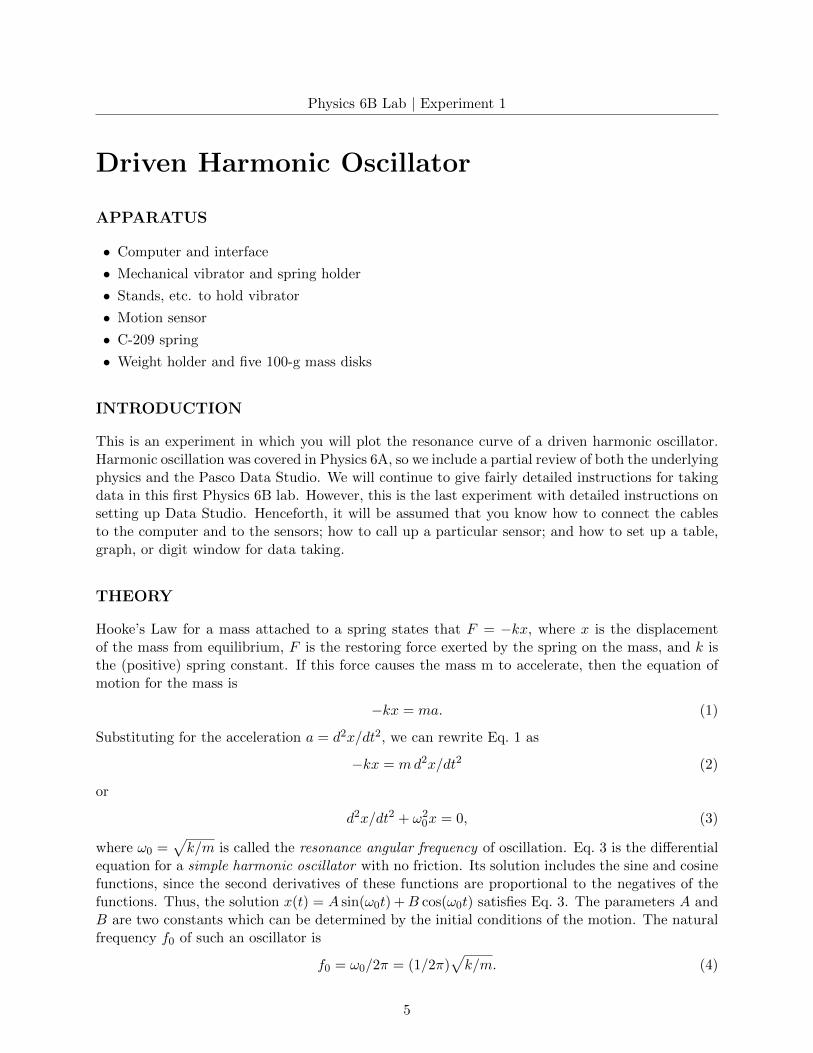
Physics texts give us the solution of Eq. 6 (and explain how it is obtained):
x(t) = A0e−bt/2m cos(ω1t+ φ). (7)
The parameter A0 is the initial amplitude of the oscillations, and φ is the phase angle; these two con-stants are determined by the initial conditions of the motion. The oscillations decay exponentiallyin time, as shown in the figure below:
In addition, the angular frequency of oscillation is shifted slightly to
ω1 =√k/m− (b/2m)2 =
√ω20 − (b/2m)2. (8)
Now imagine that an external force which varies cosinusoidally (or sinusoidally) in time is appliedto the mass at an arbitrary angular frequency ω2. The resultant behavior of the mass is known asdriven harmonic motion. The mass vibrates with a relatively small amplitude, unless the drivingangular frequency ω2 is near the resonance angular frequency ω0. In this case, the amplitude
6
Physics 6B Lab | Experiment 1
becomes very large. If the external force has the form Fm cos(ω2t), then our equation for the drivenharmonic oscillator can be written as
−kx− b dx/dt+ Fm cos(ω2t) = md2x/dt2 (9)
or
md2x/dt2 + b dx/dt+ kx = Fm cos(ω2t). (10)
The solution of Eq. 10 can also be found in physics texts:
x(t) = (Fm/G) cos(ω2t+ φ), (11)
where
G =√m2(ω2
2 − ω20)2 + b2ω2
2 (12)
and
φ = cos−1(bω2/G). (13)
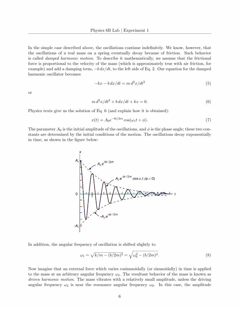
The factor G in the denominator of Eq. 11 determines the shape of the resonance curve, whichwe wish to measure in this experiment. When the driving angular frequency ω2 is close to theresonance angular frequency ω0, G is small, and the amplitude of oscillation becomes large. Whenthe driving angular frequency ω2 is far from the resonance angular frequency ω0, G is large, andthe amplitude of oscillation is small.
This is the curve we wish to measure in the experiment.
THE QUALITY FACTOR
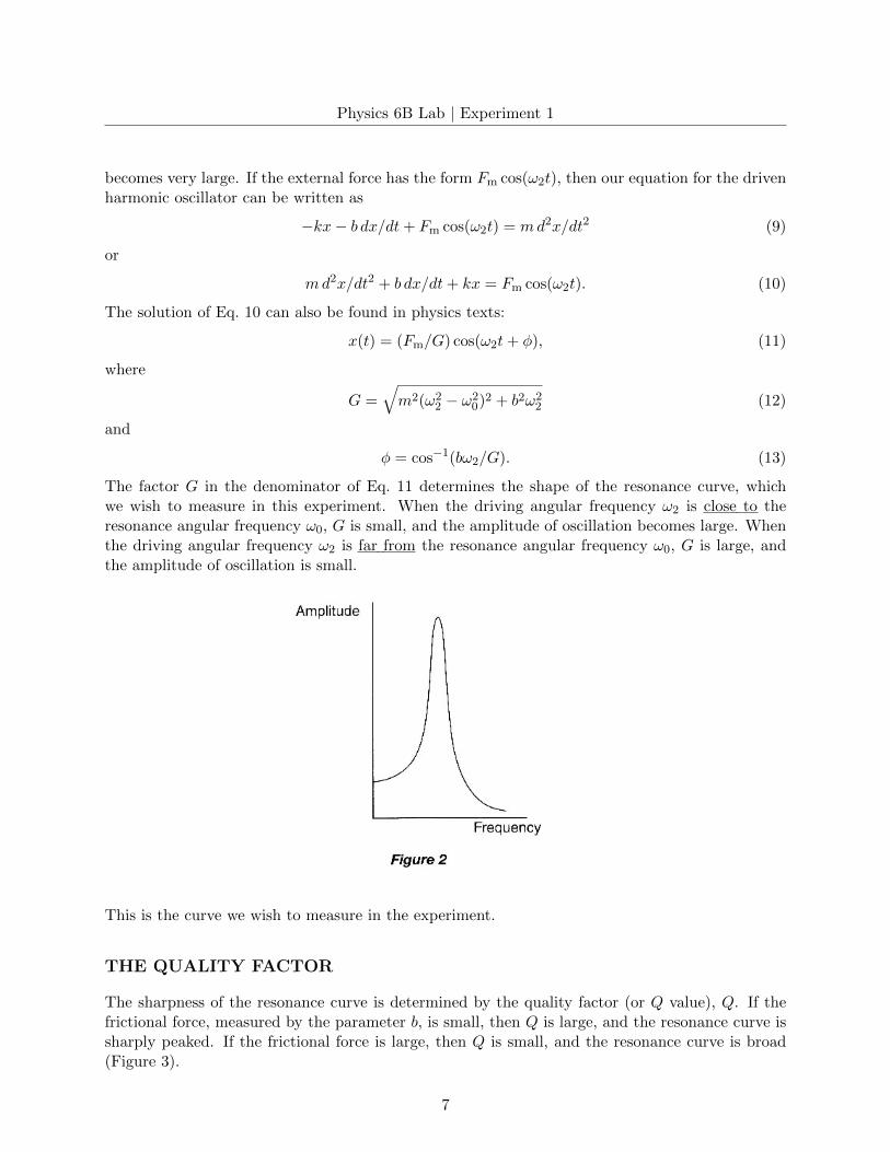
The sharpness of the resonance curve is determined by the quality factor (or Q value), Q. If thefrictional force, measured by the parameter b, is small, then Q is large, and the resonance curve issharply peaked. If the frictional force is large, then Q is small, and the resonance curve is broad(Figure 3).
7
Physics 6B Lab | Experiment 1
The general definition of Q is
Q = 2π × (energy stored) / (energy dissipated in one cycle). (14)
(If the energy dissipated per cycle is small, then Q is large, and the resonance curve is sharplypeaked.) Physics texts derive the relationship between Q and the motion parameters,
Q = mω1/b, (15)
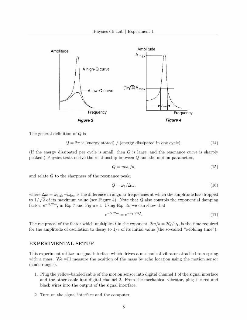
and relate Q to the sharpness of the resonance peak,
Q = ω1/∆ω, (16)
where ∆ω = ωhigh−ωlow is the difference in angular frequencies at which the amplitude has droppedto 1/
√2 of its maximum value (see Figure 4). Note that Q also controls the exponential damping
factor, e−bt/2m, in Eq. 7 and Figure 1. Using Eq. 15, we can show that
e−bt/2m = e−ω1t/2Q. (17)
The reciprocal of the factor which multiplies t in the exponent, 2m/b = 2Q/ω1, is the time requiredfor the amplitude of oscillation to decay to 1/e of its initial value (the so-called “e-folding time”).
EXPERIMENTAL SETUP
This experiment utilizes a signal interface which drives a mechanical vibrator attached to a springwith a mass. We will measure the position of the mass by echo location using the motion sensor(sonic ranger).
1. Plug the yellow-banded cable of the motion sensor into digital channel 1 of the signal interfaceand the other cable into digital channel 2. From the mechanical vibrator, plug the red andblack wires into the output of the signal interface.
2. Turn on the signal interface and the computer.
8
Physics 6B Lab | Experiment 1
3. Call up PASCO Capstone. Click on “Hardware Setup” to display the interface. Click onchannel 1 of the interface and select “Motion Sensor II”. Click on the yellow circle at theoutput of the interface. This will add the Output Voltage-Current Sensor.
4. Click on “Signal Generator”. Set Waveform to Sine, set Frequency to 10 Hz, and set Ampli-tude to 1 V.
5. Click the “On” switch in the signal generator window, and check that the mechanical vibratorstem is shaking. Experiment with the up and down arrows to adjust the frequency andamplitude of the vibrations. You can also click on the number itself and type the desiredvalue. Then click “Off”.
PROCEDURE PART 1: FINDING THE NATURAL FREQUENCY
1. Attach a C-209 spring with a total mass of 450 g (400-g mass + 50-g mass holder) to thevibrator stem. Place the motion sensor on the floor under the mass-spring system.
2. In the following procedures, be very careful not to drop masses onto the motion sensor. Securethe spring holder firmly to the vibrator stem. If the vibrations become large, they might shakea mass loose. Do not leave masses unattended on the spring; set them aside immediately whenyou stop taking measurements for a while.
3. Select the “Text & Graph” option on Capstone. Click on the “Select Measurement” buttonon the y-axis of the graph. Under Motion Sensor II, click on “position”.
4. Make sure the signal generator switch is “Off” in its window. With your hand, set the massgently vibrating, click “Record”, then “Stop” after approximately 15 seconds.
5. To zoom in on your data, click on the “Scale axes to show all data” button above the graph(square with a red arrow pointing diagonally).
6. Check that you are obtaining clear oscillations on the graph. If not, adjust the positions of themotion sensor and spring vibrator accordingly. You can delete experimental runs by clickingthe drop down arrow next to “Delete Last Run”. Record a clear set of 12 – 15 oscillations.
7. Note a set of 10 clear oscillations on your graph. Record the time at the beginning of theoscillations and the time at the end of 10 complete oscillations. The frequency (number ofoscillations per second) is equal to 10 divided by the time required for 10 complete oscillations.
8. Repeat the procedure above three times, and record the average frequency. (This is sometimescalled the natural frequency.)
PROCEDURE PART 2: PLOTTING THE RESONANCE CURVE
In this section, you will verify that resonance occurs when a driving force is applied at the naturalfrequency of the oscillator.
9
Physics 6B Lab | Experiment 1
1. Set the frequency of the signal generator to your measured natural frequency and the ampli-tude to approximately 1 V. Click the “Auto” box on the signal generator window. This willautomatically turn the generator on when the “Record” button is clicked and switch it offwhen “Stop” is clicked.
2. Set the mass at rest, and click “Start”. Observe the oscillations building up. Make sure theydo not get too wild; if so, stop and reduce the amplitude of the signal generator, and startagain.
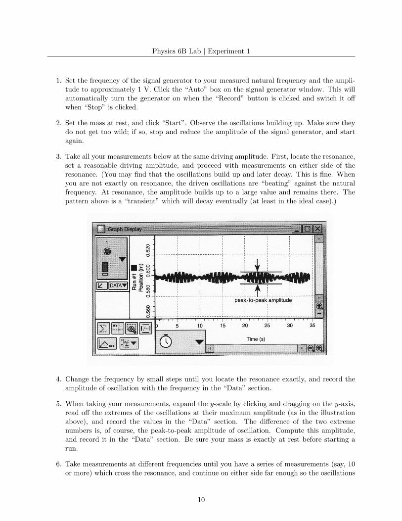
3. Take all your measurements below at the same driving amplitude. First, locate the resonance,set a reasonable driving amplitude, and proceed with measurements on either side of theresonance. (You may find that the oscillations build up and later decay. This is fine. Whenyou are not exactly on resonance, the driven oscillations are “beating” against the naturalfrequency. At resonance, the amplitude builds up to a large value and remains there. Thepattern above is a “transient” which will decay eventually (at least in the ideal case).)
4. Change the frequency by small steps until you locate the resonance exactly, and record theamplitude of oscillation with the frequency in the “Data” section.
5. When taking your measurements, expand the y-scale by clicking and dragging on the y-axis,read off the extremes of the oscillations at their maximum amplitude (as in the illustrationabove), and record the values in the “Data” section. The difference of the two extremenumbers is, of course, the peak-to-peak amplitude of oscillation. Compute this amplitude,and record it in the “Data” section. Be sure your mass is exactly at rest before starting arun.
6. Take measurements at different frequencies until you have a series of measurements (say, 10or more) which cross the resonance, and continue on either side far enough so the oscillations
10
Physics 6B Lab | Experiment 1
are quite small compared to the maximum at resonance. Use small frequency steps with theup and down arrows near the resonance to map it accurately and obtain a nice smooth curve.You can adjust the number of decimal places by clicking on the left and right arrows near thefrequency setting.
7. When you have a good series of measurements across the resonance, make a careful plot ofthe resonance curve in Excel. Always title your graph and label the axes. Show your workto the TA. You have completed the required part of the experiment. The next steps result invarying degrees of additional credit.
DATA
Procedure Part 1:
8. Frequency (Trial 1) =
Frequency (Trial 2) =
Frequency (Trial 3) =
9. Average frequency =
Procedure Part 2:
5. Amplitude =
Frequency =
6. Maximum position =
Minimum position =
Peak-to-peak amplitude =
7. Maximum positions =
11
Physics 6B Lab | Experiment 1
Minimum positions =
Peak-to-peak amplitudes =
8. Plot the resonance curve using Excel. Remember to label the axes and title the graph.
12
Physics 6B Lab | Experiment 1
ADDITIONAL CREDIT PART 1: FINDING THE SPRING CONSTANT (2mills)
We determined the spring constant k for springs several times in the Physics 6A lab by using ameter stick and a set of masses, entering the measurements into Excel, and finding the slope of theline.
Here is an alternate method. Use the motion sensor to take the position measurements. Get ridof any previous data runs by clicking the drop down arrow under “Delete Last Run” and clicking“Delete All Runs”. Drag a table symbol over to your work space. Click the “Select Measurement”button and choose “Position”. Make sure that the Signal Generator is in the “Off” setting and not“Auto”.
Change the recording mode from “Continuous Mode” to “Keep Mode” at the bottom of the screen.Start with only one of the five masses on the hanger. With the spring system still directly abovethe motion sensor, click “Preview”. With the mass at rest, click the “Keep Sample” button. Addanother mass and click the “Keep Sample” button again. Do this until you have values recordedfor 5 different masses. Click the “Stop” button.
Use these 5 values of position and the five masses you used to make a plot of force vs displacement.Use Excel to do a best-fit line to your data and determine the slope. How is the slope of yourgraph related to the spring constant? You will need to use the correct units of force (Newtons) toget k in the proper units. You could either convert each mass entry into units of force and makeyour keyboard entries in Newtons, or just proceed with mass in units of kilograms and make theconversion of units at the end when you read the slope from the curve-fitting routine. In your work,make clear which method you are using.
Slope of line =
Spring constant k =
ADDITIONAL CREDIT PART 2: PREDICTING THE RESONANCE FRE-QUENCY (1 mill)
If there were no friction, the resonance frequency would be
f0 = ω0/2π = (1/2π)√k/m. (4)
Compute this value of f0, and compare it with your measured value of the resonance frequency.Record your results clearly.
f0 (computed from Eq. 4 ) =
f0 (measured) =
Percentage difference in f0 =
13
Physics 6B Lab | Experiment 1
ADDITIONAL CREDIT PART 3: THE QUALITY FACTOR AND FRICTION(2 mills)
We saw that
Q = ω1/∆ω, (16)
where ∆ω = ωhigh−ωlow. Compute the value of Q for your mass on a spring by finding the angularfrequencies on your resonance curve where the amplitude has dropped to 1/
√2 of its maximum
value.
Q is also equal to mω1/b, by Eq. 15. By approximating ω1 as ω0, estimate the value of b. Thencompute the true resonance angular frequency, including friction, from
ω1 =√k/m− (b/2m)2. (8)
What is the percentage difference between ω1 and ω0? Could your measurements of the resonancecurve have distinguished between ω1 and ω0?
ωhigh =
ωlow =
Q =
b =
ω1 =
Percentage difference between ω1 and ω0 =
14
Physics 6B Lab | Experiment 2
Standing Waves
APPARATUS
• Computer and interface
• Mechanical vibrator
• Clip from vibrator to string
• Three strings of different densities
• Meter stick clamped vertically to measure vibration amplitudes
• Weight set
• Acculab digital scale
INTRODUCTION
Have you ever wondered why pressing different positions on your guitar string produces differentpitches or sounds? Or why the same sound is produced by pressing certain positions on two ormore strings? By exploring several basic properties of standing waves, you will be able to answersome of these questions. In this experiment, you will study standing waves on a string and discoverhow different modes of vibration depend on the frequency, as well as how the wave speed dependson the tension in the string.
THEORY: FORMATION OF STANDING WAVES
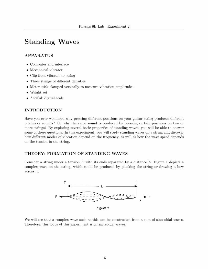
Consider a string under a tension F with its ends separated by a distance L. Figure 1 depicts acomplex wave on the string, which could be produced by plucking the string or drawing a bowacross it.
We will see that a complex wave such as this can be constructed from a sum of sinusoidal waves.Therefore, this focus of this experiment is on sinusoidal waves.
15
Physics 6B Lab | Experiment 2
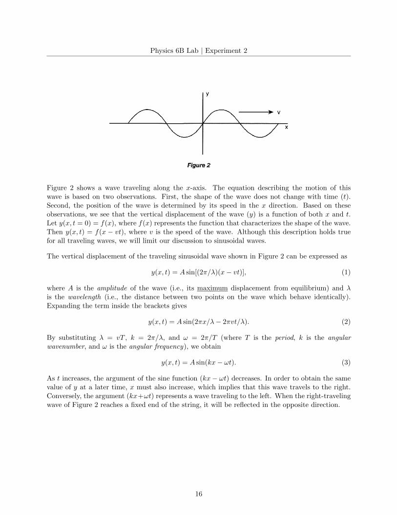
Figure 2 shows a wave traveling along the x-axis. The equation describing the motion of thiswave is based on two observations. First, the shape of the wave does not change with time (t).Second, the position of the wave is determined by its speed in the x direction. Based on theseobservations, we see that the vertical displacement of the wave (y) is a function of both x and t.Let y(x, t = 0) = f(x), where f(x) represents the function that characterizes the shape of the wave.Then y(x, t) = f(x − vt), where v is the speed of the wave. Although this description holds truefor all traveling waves, we will limit our discussion to sinusoidal waves.
The vertical displacement of the traveling sinusoidal wave shown in Figure 2 can be expressed as
y(x, t) = A sin[(2π/λ)(x− vt)], (1)
where A is the amplitude of the wave (i.e., its maximum displacement from equilibrium) and λis the wavelength (i.e., the distance between two points on the wave which behave identically).Expanding the term inside the brackets gives
y(x, t) = A sin(2πx/λ− 2πvt/λ). (2)
By substituting λ = vT , k = 2π/λ, and ω = 2π/T (where T is the period, k is the angularwavenumber, and ω is the angular frequency), we obtain
y(x, t) = A sin(kx− ωt). (3)
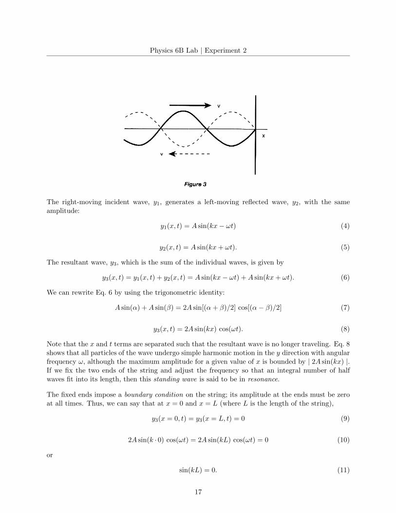
As t increases, the argument of the sine function (kx− ωt) decreases. In order to obtain the samevalue of y at a later time, x must also increase, which implies that this wave travels to the right.Conversely, the argument (kx+ωt) represents a wave traveling to the left. When the right-travelingwave of Figure 2 reaches a fixed end of the string, it will be reflected in the opposite direction.
16
Physics 6B Lab | Experiment 2
The right-moving incident wave, y1, generates a left-moving reflected wave, y2, with the sameamplitude:
y1(x, t) = A sin(kx− ωt) (4)
y2(x, t) = A sin(kx+ ωt). (5)
The resultant wave, y3, which is the sum of the individual waves, is given by
y3(x, t) = y1(x, t) + y2(x, t) = A sin(kx− ωt) +A sin(kx+ ωt). (6)
We can rewrite Eq. 6 by using the trigonometric identity:
A sin(α) +A sin(β) = 2A sin[(α+ β)/2] cos[(α− β)/2] (7)
y3(x, t) = 2A sin(kx) cos(ωt). (8)
Note that the x and t terms are separated such that the resultant wave is no longer traveling. Eq. 8shows that all particles of the wave undergo simple harmonic motion in the y direction with angularfrequency ω, although the maximum amplitude for a given value of x is bounded by | 2A sin(kx) |.If we fix the two ends of the string and adjust the frequency so that an integral number of halfwaves fit into its length, then this standing wave is said to be in resonance.
The fixed ends impose a boundary condition on the string; its amplitude at the ends must be zeroat all times. Thus, we can say that at x = 0 and x = L (where L is the length of the string),
y3(x = 0, t) = y3(x = L, t) = 0 (9)
2A sin(k · 0) cos(ωt) = 2A sin(kL) cos(ωt) = 0 (10)
or
sin(kL) = 0. (11)
17
Physics 6B Lab | Experiment 2
Eq. 11 is a boundary condition which restricts the string to certain modes of vibration. Thisequation is satisfied only when kL = nπ, where n is the index of vibration and is equal to anypositive integer. In other words, the possible values of k and λ for any given L are
kL = (2π/λ)L = nπ (n = 1, 2, 3, . . .) (12)
or
λ = 2L/n. (13)
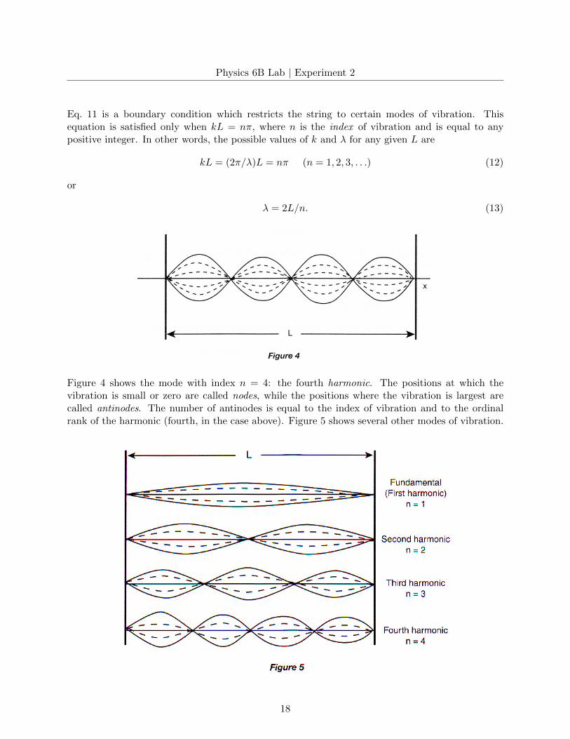
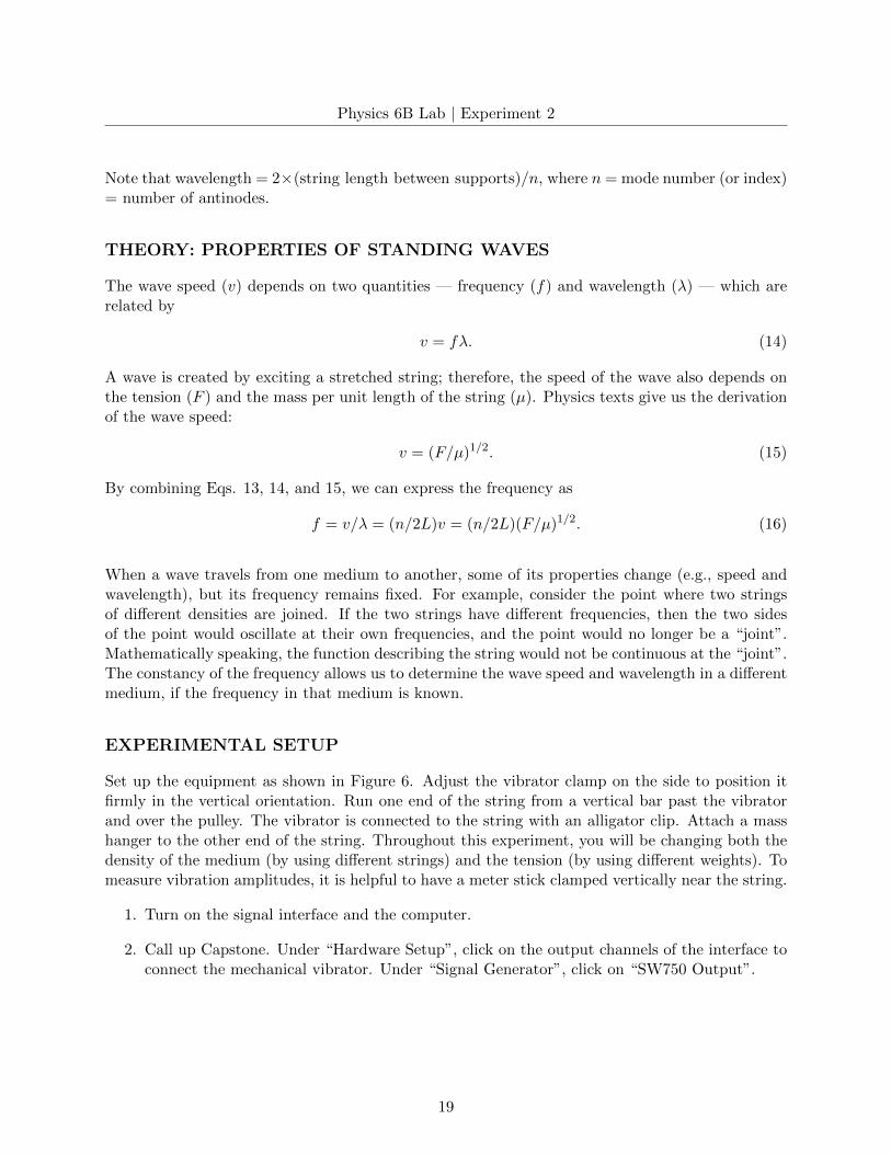
Figure 4 shows the mode with index n = 4: the fourth harmonic. The positions at which thevibration is small or zero are called nodes, while the positions where the vibration is largest arecalled antinodes. The number of antinodes is equal to the index of vibration and to the ordinalrank of the harmonic (fourth, in the case above). Figure 5 shows several other modes of vibration.
18
Physics 6B Lab | Experiment 2
Note that wavelength = 2×(string length between supports)/n, where n = mode number (or index)= number of antinodes.
THEORY: PROPERTIES OF STANDING WAVES
The wave speed (v) depends on two quantities — frequency (f) and wavelength (λ) — which arerelated by
v = fλ. (14)
A wave is created by exciting a stretched string; therefore, the speed of the wave also depends onthe tension (F ) and the mass per unit length of the string (µ). Physics texts give us the derivationof the wave speed:
v = (F/µ)1/2. (15)
By combining Eqs. 13, 14, and 15, we can express the frequency as
f = v/λ = (n/2L)v = (n/2L)(F/µ)1/2. (16)
When a wave travels from one medium to another, some of its properties change (e.g., speed andwavelength), but its frequency remains fixed. For example, consider the point where two stringsof different densities are joined. If the two strings have different frequencies, then the two sidesof the point would oscillate at their own frequencies, and the point would no longer be a “joint”.Mathematically speaking, the function describing the string would not be continuous at the “joint”.The constancy of the frequency allows us to determine the wave speed and wavelength in a differentmedium, if the frequency in that medium is known.
EXPERIMENTAL SETUP
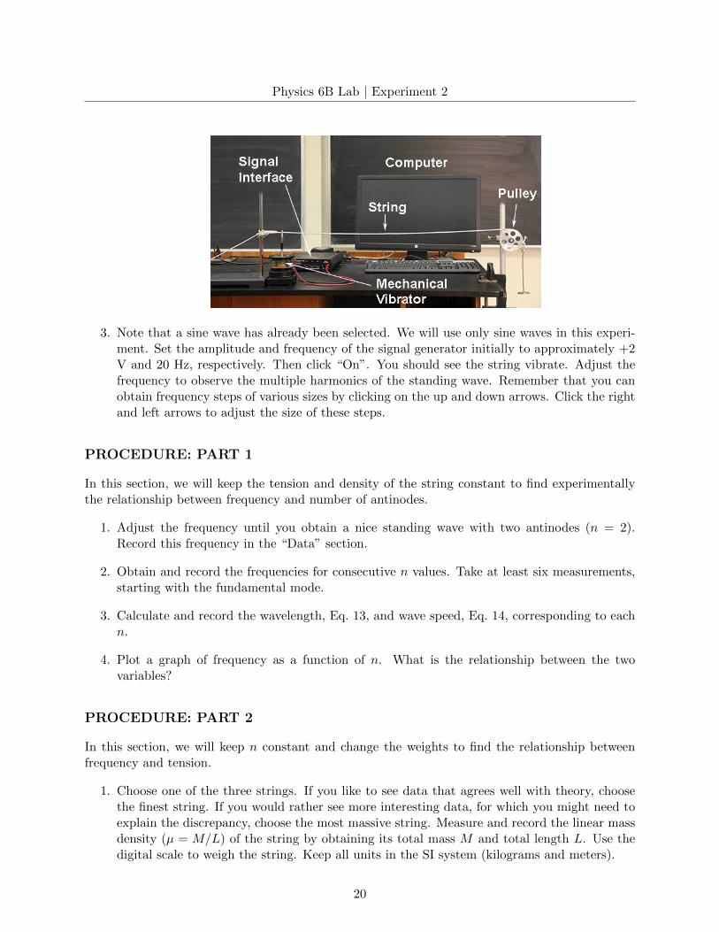
Set up the equipment as shown in Figure 6. Adjust the vibrator clamp on the side to position itfirmly in the vertical orientation. Run one end of the string from a vertical bar past the vibratorand over the pulley. The vibrator is connected to the string with an alligator clip. Attach a masshanger to the other end of the string. Throughout this experiment, you will be changing both thedensity of the medium (by using different strings) and the tension (by using different weights). Tomeasure vibration amplitudes, it is helpful to have a meter stick clamped vertically near the string.
1. Turn on the signal interface and the computer.
2. Call up Capstone. Under “Hardware Setup”, click on the output channels of the interface toconnect the mechanical vibrator. Under “Signal Generator”, click on “SW750 Output”.
19
Physics 6B Lab | Experiment 2
3. Note that a sine wave has already been selected. We will use only sine waves in this experi-ment. Set the amplitude and frequency of the signal generator initially to approximately +2V and 20 Hz, respectively. Then click “On”. You should see the string vibrate. Adjust thefrequency to observe the multiple harmonics of the standing wave. Remember that you canobtain frequency steps of various sizes by clicking on the up and down arrows. Click the rightand left arrows to adjust the size of these steps.
PROCEDURE: PART 1
In this section, we will keep the tension and density of the string constant to find experimentallythe relationship between frequency and number of antinodes.
1. Adjust the frequency until you obtain a nice standing wave with two antinodes (n = 2).Record this frequency in the “Data” section.
2. Obtain and record the frequencies for consecutive n values. Take at least six measurements,starting with the fundamental mode.
3. Calculate and record the wavelength, Eq. 13, and wave speed, Eq. 14, corresponding to eachn.
4. Plot a graph of frequency as a function of n. What is the relationship between the twovariables?
PROCEDURE: PART 2
In this section, we will keep n constant and change the weights to find the relationship betweenfrequency and tension.
1. Choose one of the three strings. If you like to see data that agrees well with theory, choosethe finest string. If you would rather see more interesting data, for which you might need toexplain the discrepancy, choose the most massive string. Measure and record the linear massdensity (µ = M/L) of the string by obtaining its total mass M and total length L. Use thedigital scale to weigh the string. Keep all units in the SI system (kilograms and meters).
20
Physics 6B Lab | Experiment 2
2. Using the 50-g mass hanger, measure and record the frequency for the n = 2 mode. (Note:You may choose any integer for n, but remember to keep n constant throughout the rest ofthis section.)
3. Add masses in increments of 50 g, and adjust the frequency so that the same number of nodesis obtained. Take and record measurements for at least six different tensions.
4. The wave speed should be related to the tension F and linear mass density µ by v = (F/µ)1/2.Calculate and record the wave speed in each case using Eq. 14, and plot v2 as a function ofF/µ. (You have calculated v2 from the frequency and wavelength; these are the y-axis values.You have calculated F/µ from the measured tension and linear mass density; these are thex-axis values. Be sure to convert the tension into units of Newtons.) You now have theexperimental points.
5. Now plot the “theoretical” line v2 = F/µ. This is a straight line at 450 on your graph, if youused the same scale on both axes. Do your experimental and theoretical results agree well?If not, what might be the reasons?
PROCEDURE: PART 3
In this section, we will determine the relationship between frequency and the density of a mediumthrough which a wave propagates.
1. Measure the linear mass densities (µ = M/L) of the two other strings as described above.
2. Keeping the tension and mode number constant at, say, 100 g and n = 2, measure and recordthe frequencies for the three strings.
3. Calculate and record the “experimental” wave speed from the frequency and wavelength foreach string density.
4. Calculate and record the “theoretical” wave speed for each string density from v = (F/µ)1/2,and compare these speeds with the experimental values.
DATA
Procedure Part 1:
1. Frequency (n = 2 mode) =
2. Frequency (n = 1 mode) =
Frequency (n = 2 mode) =
Frequency (n = 3 mode) =
Frequency (n = 4 mode) =
21
Physics 6B Lab | Experiment 2
Frequency (n = 5 mode) =
Frequency (n = 6 mode) =
3. Wavelength (n = 1 mode) =
Wave speed (n = 1 mode) =
Wavelength (n = 2 mode) =
Wave speed (n = 2 mode) =
Wavelength (n = 3 mode) =
Wave speed (n = 3 mode) =
Wavelength (n = 4 mode) =
Wave speed (n = 4 mode) =
Wavelength (n = 5 mode) =
Wave speed (n = 5 mode) =
Wavelength (n = 6 mode) =
Wave speed (n = 6 mode) =
4. Plot the graph of the frequency as a function of n using one sheet of graph paper at the endof this workbook. Remember to label the axes and title the graph.
Procedure Part 2:
1. Mass of string 1 =
Length of string 1 =
2. Frequency (with 50-g mass) =
3. Frequency (with 100-g mass) =
Frequency (with 150-g mass) =
Frequency (with 200-g mass) =
Frequency (with 250-g mass) =
Frequency (with 300-g mass) =
Frequency (with 350-g mass) =
22
Physics 6B Lab | Experiment 2
4. Wave speed (with 50-g mass) =
Wave speed (with 100-g mass) =
Wave speed (with 150-g mass) =
Wave speed (with 200-g mass) =
Wave speed (with 250-g mass) =
Wave speed (with 300-g mass) =
Wave speed (with 350-g mass) =
Plot the experiment graph of v2 as a function of F/µ using one sheet of graph paper at theend of this workbook. Remember to label the axes and title the graph.
5. Plot the theoretical graph of v2 as a function of F/µ using the same sheet of graph paper.Remember to label the axes and title the graph.
Procedure Part 3:
1. Mass of string 2 =
Length of string 2 =
Mass of string 3 =
Length of string 3 =
2. Frequency (string 1) =
Frequency (string 2) =
Frequency (string 3) =
3. Experimental wave speed (string 1) =
Experimental wave speed (string 2) =
Experimental wave speed (string 3) =
4. Theoretical wave speed (string 1) =
Theoretical wave speed (string 2) =
Theoretical wave speed (string 3) =
Percentage difference between experimental and theoretical speeds (string 1) =
23
Physics 6B Lab | Experiment 2
Percentage difference between experimental and theoretical speeds (string 2) =
Percentage difference between experimental and theoretical speeds (string 3) =
ADDITIONAL CREDIT PART 1 (1 mill)
Carefully write out a complete answer to the question posed at the beginning of the experiment:Why does pressing different positions on your guitar string produce different pitches?
ADDITIONAL CREDIT PART 2 (2 mills)
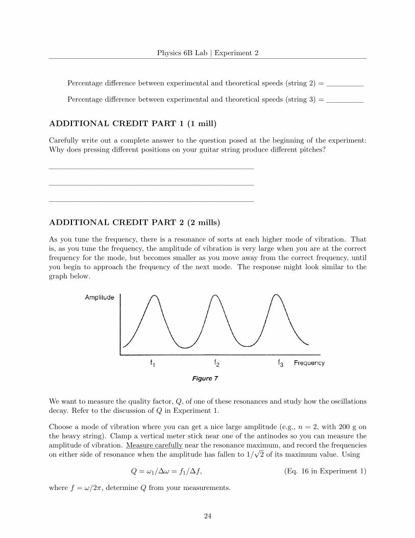
As you tune the frequency, there is a resonance of sorts at each higher mode of vibration. Thatis, as you tune the frequency, the amplitude of vibration is very large when you are at the correctfrequency for the mode, but becomes smaller as you move away from the correct frequency, untilyou begin to approach the frequency of the next mode. The response might look similar to thegraph below.
We want to measure the quality factor, Q, of one of these resonances and study how the oscillationsdecay. Refer to the discussion of Q in Experiment 1.
Choose a mode of vibration where you can get a nice large amplitude (e.g., n = 2, with 200 g onthe heavy string). Clamp a vertical meter stick near one of the antinodes so you can measure theamplitude of vibration. Measure carefully near the resonance maximum, and record the frequencieson either side of resonance when the amplitude has fallen to 1/
√2 of its maximum value. Using
Q = ω1/∆ω = f1/∆f, (Eq. 16 in Experiment 1)
where f = ω/2π, determine Q from your measurements.
24
Physics 6B Lab | Experiment 2
As discussed in Experiment 1 in connection with its Eq. (16), Q also controls the damping rateof the vibration. Start the wave motion until it builds up to full amplitude. Then switch off thedriving vibrator, and observe the wave motion decay. Measure the full amplitude Amax of vibrationat resonance by reading off distances from the meter stick while the vibrator is driving the wave,and calculate Amax/e (e = 2.718 . . .). Devise a way to note this reduced amplitude on the meterstick.
Start the wave again at full amplitude, switch off the drive, and measure the time required for theamplitude to decay to Amax/e (the so-called “e-folding time”). Compare this time with 2Q/ω1 =Q/πf1, and record the results below.
Amplitude at resonance (Amax) =
Amax
√2 =
Frequencies at which amplitude is equal to Amax
√2 =
Difference in frequencies (∆f) =
Q =
Amax/e =
Time required for amplitude to decay to Amax/e =
2Q/ω1 =
25
Physics 6B Lab | Experiment 3
Electrostatics
APPARATUS
• Heat lamp
• Timer
• Two Lucite rods
• Rough plastic rod
• Silk
• Cat fur
• Stand with stirrup holder
• Pith balls on hanger
• Electroscope
• Electrophorus
• Coulomb’s Law (charging pads not needed)
INTRODUCTION
This experiment consists of many short demonstrations in electrostatics. In most of the exercises,you do not take data, but record a short description of your observations. If high-humidity condi-tions prevent you from completing certain parts, you may try them again next week with the Vande Graaff experiments.
THEORY
The fundamental concept in electrostatics is electrical charge. We are all familiar with the fact thatrubbing two materials together — for example, a rubber comb on cat fur — produces a “static”charge. This process is called charging by friction. Surprisingly, the exact physics of the process ofcharging by friction is poorly understood. However, it is known that the making and breaking ofcontact between the two materials transfers the charge.
The charged particles which make up the universe come in three kinds: positive, negative, andneutral. Neutral particles do not interact with electrical forces. Charged particles exert electricaland magnetic forces on one another, but if the charges are stationary, the mutual force is verysimple in form and is given by Coulomb’s Law:
FE = kqQ/r2, (1)
where FE is the electrical force between any two stationary charged particles with charges q and Q(measured in coulombs), r is the separation between the charges (measured in meters), and k is aconstant of nature (equal to 9×10⁹ Nm2/C2 in SI units).
26
Physics 6B Lab | Experiment 3
The study of the Coulomb forces among arrangements of stationary charged particles is calledelectrostatics. Coulomb’s Law describes three properties of the electrical force:
1. The force is inversely proportional to the square of the distance between the charges, and isdirected along the straight line that connects their centers.
2. The force is proportional to the product of the magnitude of the charges.
3. Two particles of the same charge exert a repulsive force on each other, and two particles ofopposite charge exert an attractive force on each other.
Most of the common objects we deal with in the macroscopic (human-sized) world are electri-cally neutral. They are composed of atoms that consist of negatively charged electrons moving inquantum motion around a positively charged nucleus. The total negative charge of the electronsis normally exactly equal to the total positive charge of the nuclei, so the atoms (and thereforethe entire object) have no net electrical charge. When we charge a material by friction, we aretransferring some of the electrons from one material to another.
Materials such as metals are conductors. Each metal atom contributes one or two electrons thatcan move relatively freely through the material. A conductor will carry an electrical current. Othermaterials such as glass are insulators. Their electrons are bound tightly and cannot move. Chargesticks on an insulator, but does not move freely through it.
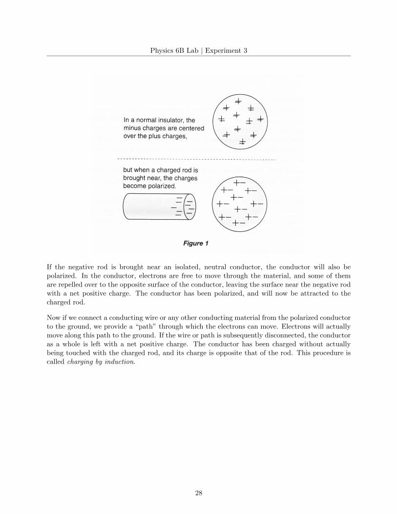
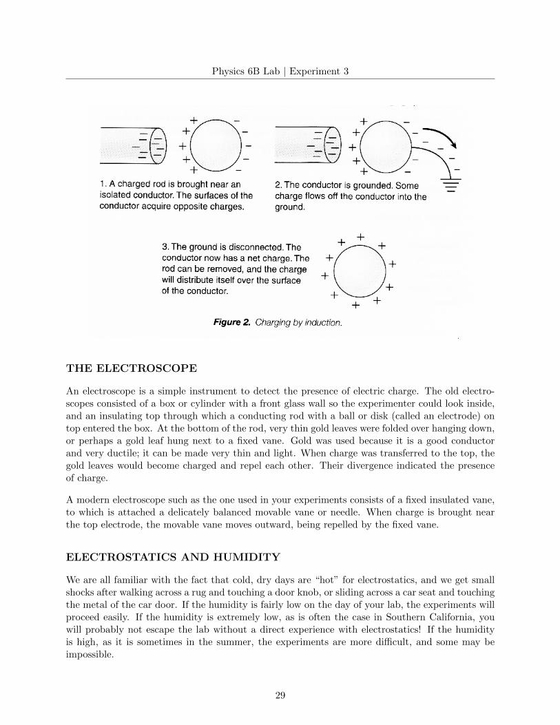
A neutral particle is not affected by electrical forces. Nevertheless, a charged object will attract aneutral macroscopic object by the process of electrical polarization. For example, if a negativelycharged rod is brought close to an isolated, neutral insulator, the electrons in the atoms of theinsulator will be pushed slightly away from the negative rod, and the positive nuclei will be attractedslightly toward the negative rod. We say that the rod has induced polarization in the insulator, butits net charge is still zero. The polarization of charge in the insulator is small, but now its positivecharge is a bit closer to the negative rod, and its negative charge is a bit farther away. Thus, thepositive charge is attracted to the rod more strongly than the negative charge is repelled, and thereis an overall net attraction. (Do not confuse electrical polarization with the polarization of light,which is an entirely different phenomenon.)
27
Physics 6B Lab | Experiment 3
If the negative rod is brought near an isolated, neutral conductor, the conductor will also bepolarized. In the conductor, electrons are free to move through the material, and some of themare repelled over to the opposite surface of the conductor, leaving the surface near the negative rodwith a net positive charge. The conductor has been polarized, and will now be attracted to thecharged rod.
Now if we connect a conducting wire or any other conducting material from the polarized conductorto the ground, we provide a “path” through which the electrons can move. Electrons will actuallymove along this path to the ground. If the wire or path is subsequently disconnected, the conductoras a whole is left with a net positive charge. The conductor has been charged without actuallybeing touched with the charged rod, and its charge is opposite that of the rod. This procedure iscalled charging by induction.
28
Physics 6B Lab | Experiment 3
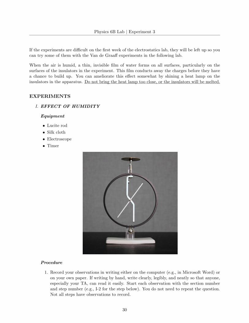
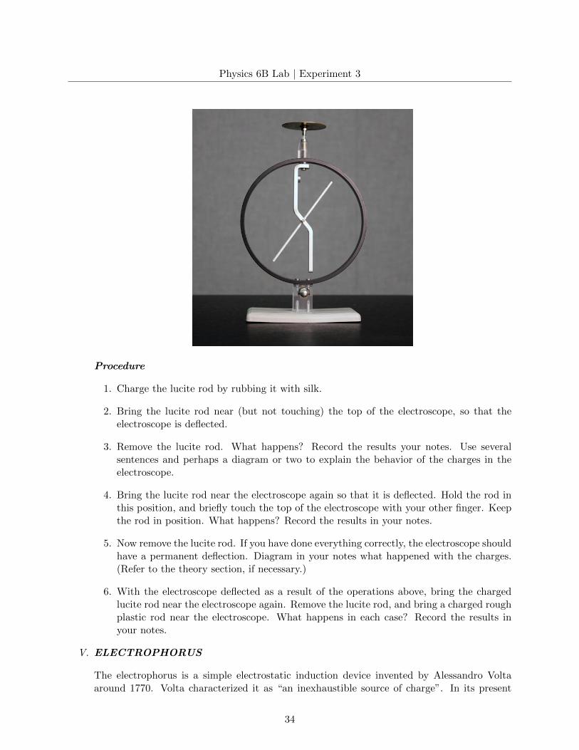
THE ELECTROSCOPE
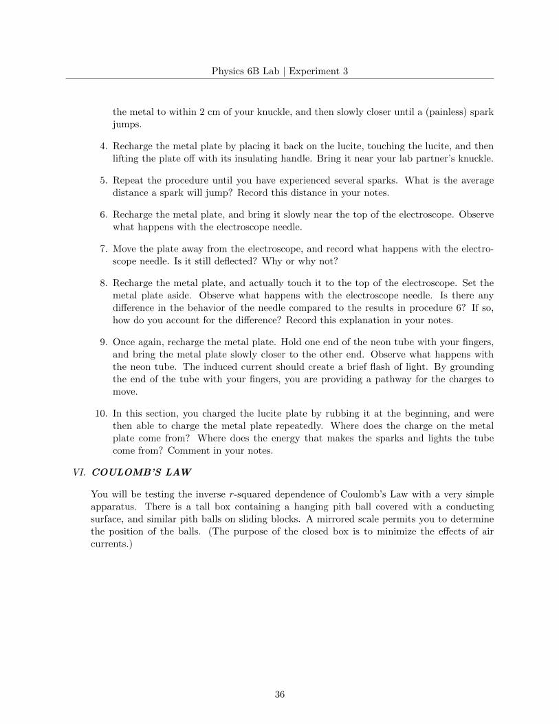
An electroscope is a simple instrument to detect the presence of electric charge. The old electro-scopes consisted of a box or cylinder with a front glass wall so the experimenter could look inside,and an insulating top through which a conducting rod with a ball or disk (called an electrode) ontop entered the box. At the bottom of the rod, very thin gold leaves were folded over hanging down,or perhaps a gold leaf hung next to a fixed vane. Gold was used because it is a good conductorand very ductile; it can be made very thin and light. When charge was transferred to the top, thegold leaves would become charged and repel each other. Their divergence indicated the presenceof charge.
A modern electroscope such as the one used in your experiments consists of a fixed insulated vane,to which is attached a delicately balanced movable vane or needle. When charge is brought nearthe top electrode, the movable vane moves outward, being repelled by the fixed vane.
ELECTROSTATICS AND HUMIDITY
We are all familiar with the fact that cold, dry days are “hot” for electrostatics, and we get smallshocks after walking across a rug and touching a door knob, or sliding across a car seat and touchingthe metal of the car door. If the humidity is fairly low on the day of your lab, the experiments willproceed easily. If the humidity is extremely low, as is often the case in Southern California, youwill probably not escape the lab without a direct experience with electrostatics! If the humidityis high, as it is sometimes in the summer, the experiments are more difficult, and some may beimpossible.
29
Physics 6B Lab | Experiment 3
If the experiments are difficult on the first week of the electrostatics lab, they will be left up so youcan try some of them with the Van de Graaff experiments in the following lab.
When the air is humid, a thin, invisible film of water forms on all surfaces, particularly on thesurfaces of the insulators in the experiment. This film conducts away the charges before they havea chance to build up. You can ameliorate this effect somewhat by shining a heat lamp on theinsulators in the apparatus. Do not bring the heat lamp too close, or the insulators will be melted.
EXPERIMENTS
I. EFFECT OF HUMIDITY
Equipment
• Lucite rod
• Silk cloth
• Electroscope
• Timer
Procedure
1. Record your observations in writing either on the computer (e.g., in Microsoft Word) oron your own paper. If writing by hand, write clearly, legibly, and neatly so that anyone,especially your TA, can read it easily. Start each observation with the section numberand step number (e.g., I-2 for the step below). You do not need to repeat the question.Not all steps have observations to record.
30
Physics 6B Lab | Experiment 3
2. Record in your notes the relative humidity in the room (from the wall meter) and theinside and outside temperature.
3. For this experiment, do not shine the flood lamp on the electroscope. Be prepared tostart your timer. You may use the stopwatch function of your wristwatch.
4. Rub the lucite rod vigorously with the silk cloth. Use a little whipping motion at the endof the rubbing. Touch the lucite rod to the top of the electroscope. Move the rod alongand around the top so you touch as much of its surface to the metal of the electroscopeas possible. Since the rod is an insulator, charge will not flow from all parts of the rodonto the electroscope; you need to touch all parts (except where you are holding it) tothe electroscope. Start your timer immediately after charging the electroscope.
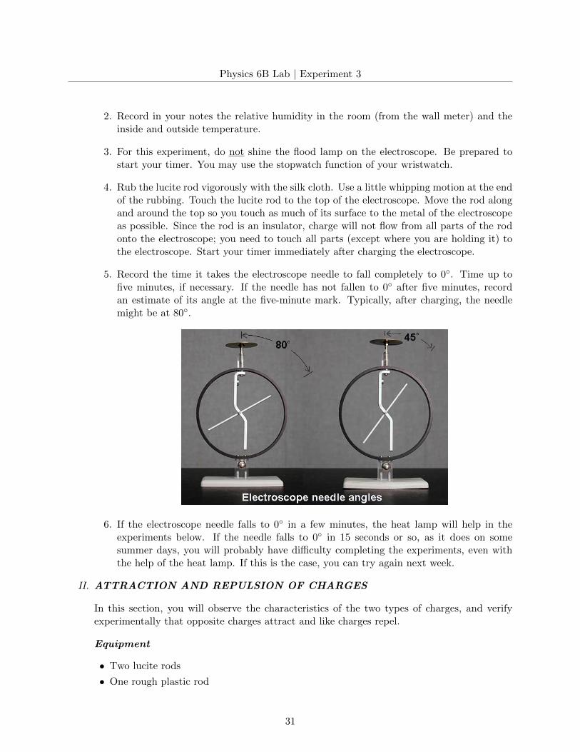
5. Record the time it takes the electroscope needle to fall completely to 0. Time up tofive minutes, if necessary. If the needle has not fallen to 0 after five minutes, recordan estimate of its angle at the five-minute mark. Typically, after charging, the needlemight be at 80.
6. If the electroscope needle falls to 0 in a few minutes, the heat lamp will help in theexperiments below. If the needle falls to 0 in 15 seconds or so, as it does on somesummer days, you will probably have difficulty completing the experiments, even withthe help of the heat lamp. If this is the case, you can try again next week.
II. ATTRACTION AND REPULSION OF CHARGES
In this section, you will observe the characteristics of the two types of charges, and verifyexperimentally that opposite charges attract and like charges repel.
Equipment
• Two lucite rods
• One rough plastic rod
31
Physics 6B Lab | Experiment 3
• Stand with stirrup holder
• Silk cloth
• Cat’s fur
Procedure
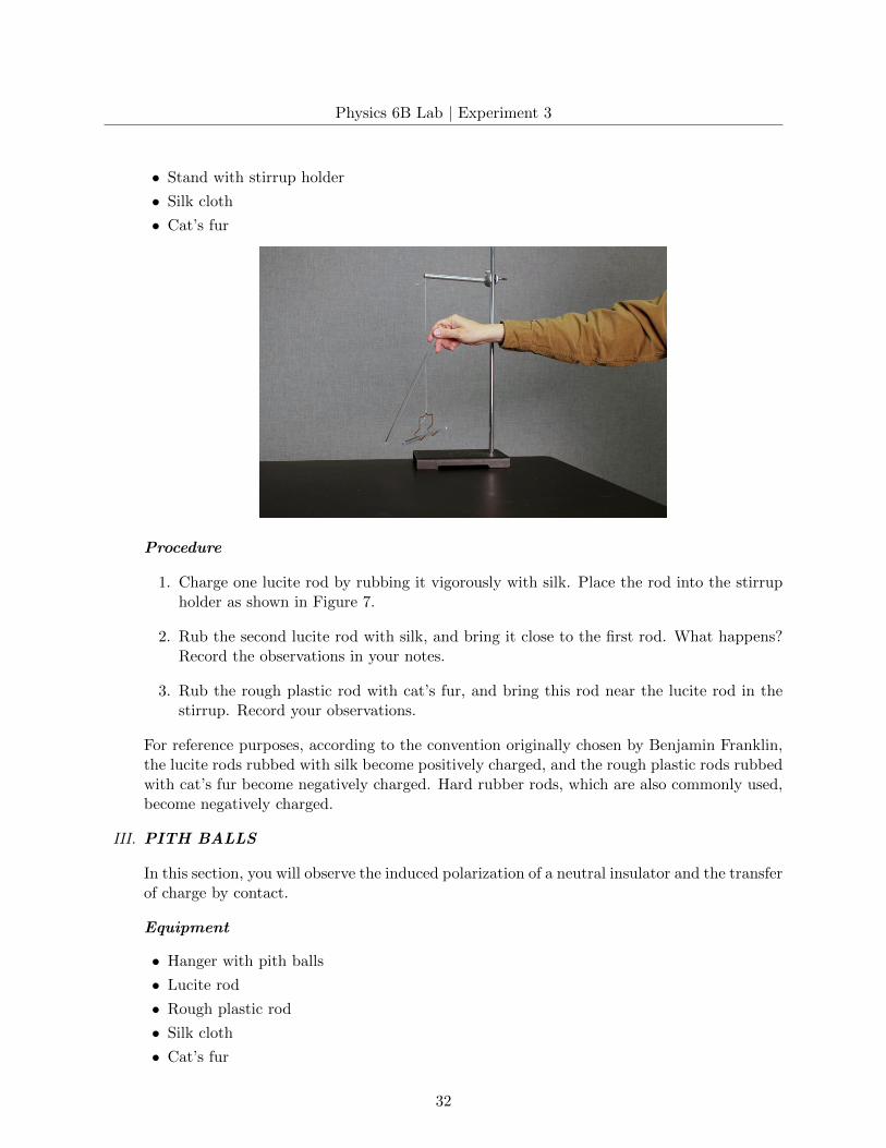
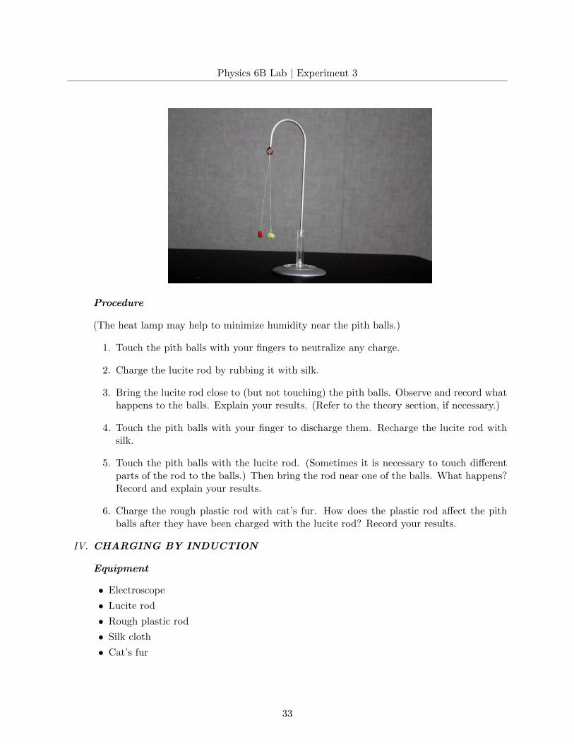
1. Charge one lucite rod by rubbing it vigorously with silk. Place the rod into the stirrupholder as shown in Figure 7.
2. Rub the second lucite rod with silk, and bring it close to the first rod. What happens?Record the observations in your notes.
3. Rub the rough plastic rod with cat’s fur, and bring this rod near the lucite rod in thestirrup. Record your observations.
For reference purposes, according to the convention originally chosen by Benjamin Franklin,the lucite rods rubbed with silk become positively charged, and the rough plastic rods rubbedwith cat’s fur become negatively charged. Hard rubber rods, which are also commonly used,become negatively charged.
III. PITH BALLS
In this section, you will observe the induced polarization of a neutral insulator and the transferof charge by contact.
Equipment
• Hanger with pith balls
• Lucite rod
• Rough plastic rod
• Silk cloth
• Cat’s fur
32
Physics 6B Lab | Experiment 3
Procedure
(The heat lamp may help to minimize humidity near the pith balls.)
1. Touch the pith balls with your fingers to neutralize any charge.
2. Charge the lucite rod by rubbing it with silk.
3. Bring the lucite rod close to (but not touching) the pith balls. Observe and record whathappens to the balls. Explain your results. (Refer to the theory section, if necessary.)
4. Touch the pith balls with your finger to discharge them. Recharge the lucite rod withsilk.
5. Touch the pith balls with the lucite rod. (Sometimes it is necessary to touch differentparts of the rod to the balls.) Then bring the rod near one of the balls. What happens?Record and explain your results.
6. Charge the rough plastic rod with cat’s fur. How does the plastic rod affect the pithballs after they have been charged with the lucite rod? Record your results.
IV. CHARGING BY INDUCTION
Equipment
• Electroscope
• Lucite rod
• Rough plastic rod
• Silk cloth
• Cat’s fur
33
Physics 6B Lab | Experiment 3
Procedure
1. Charge the lucite rod by rubbing it with silk.
2. Bring the lucite rod near (but not touching) the top of the electroscope, so that theelectroscope is deflected.
3. Remove the lucite rod. What happens? Record the results your notes. Use severalsentences and perhaps a diagram or two to explain the behavior of the charges in theelectroscope.
4. Bring the lucite rod near the electroscope again so that it is deflected. Hold the rod inthis position, and briefly touch the top of the electroscope with your other finger. Keepthe rod in position. What happens? Record the results in your notes.
5. Now remove the lucite rod. If you have done everything correctly, the electroscope shouldhave a permanent deflection. Diagram in your notes what happened with the charges.(Refer to the theory section, if necessary.)
6. With the electroscope deflected as a result of the operations above, bring the chargedlucite rod near the electroscope again. Remove the lucite rod, and bring a charged roughplastic rod near the electroscope. What happens in each case? Record the results inyour notes.
V. ELECTROPHORUS
The electrophorus is a simple electrostatic induction device invented by Alessandro Voltaaround 1770. Volta characterized it as “an inexhaustible source of charge”. In its present
34
Physics 6B Lab | Experiment 3
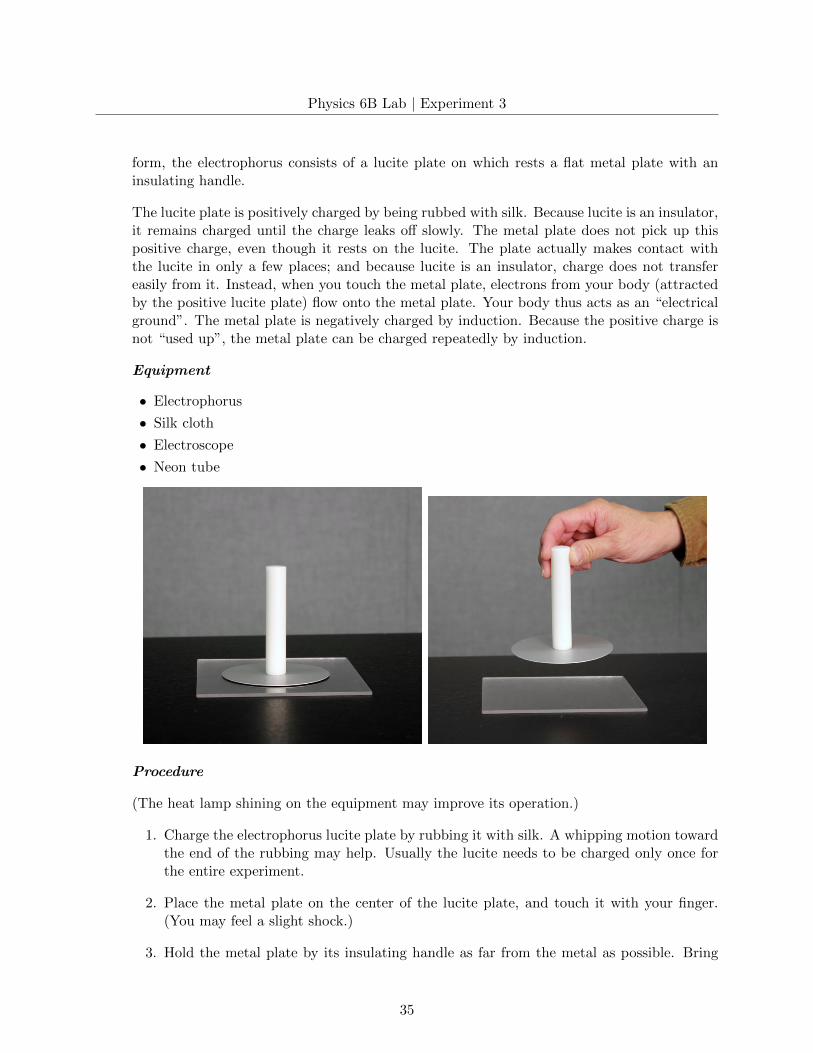
form, the electrophorus consists of a lucite plate on which rests a flat metal plate with aninsulating handle.
The lucite plate is positively charged by being rubbed with silk. Because lucite is an insulator,it remains charged until the charge leaks off slowly. The metal plate does not pick up thispositive charge, even though it rests on the lucite. The plate actually makes contact withthe lucite in only a few places; and because lucite is an insulator, charge does not transfereasily from it. Instead, when you touch the metal plate, electrons from your body (attractedby the positive lucite plate) flow onto the metal plate. Your body thus acts as an “electricalground”. The metal plate is negatively charged by induction. Because the positive charge isnot “used up”, the metal plate can be charged repeatedly by induction.
Equipment
• Electrophorus
• Silk cloth
• Electroscope
• Neon tube
Procedure
(The heat lamp shining on the equipment may improve its operation.)
1. Charge the electrophorus lucite plate by rubbing it with silk. A whipping motion towardthe end of the rubbing may help. Usually the lucite needs to be charged only once forthe entire experiment.
2. Place the metal plate on the center of the lucite plate, and touch it with your finger.(You may feel a slight shock.)
3. Hold the metal plate by its insulating handle as far from the metal as possible. Bring
35
Physics 6B Lab | Experiment 3
the metal to within 2 cm of your knuckle, and then slowly closer until a (painless) sparkjumps.
4. Recharge the metal plate by placing it back on the lucite, touching the lucite, and thenlifting the plate off with its insulating handle. Bring it near your lab partner’s knuckle.
5. Repeat the procedure until you have experienced several sparks. What is the averagedistance a spark will jump? Record this distance in your notes.
6. Recharge the metal plate, and bring it slowly near the top of the electroscope. Observewhat happens with the electroscope needle.
7. Move the plate away from the electroscope, and record what happens with the electro-scope needle. Is it still deflected? Why or why not?
8. Recharge the metal plate, and actually touch it to the top of the electroscope. Set themetal plate aside. Observe what happens with the electroscope needle. Is there anydifference in the behavior of the needle compared to the results in procedure 6? If so,how do you account for the difference? Record this explanation in your notes.
9. Once again, recharge the metal plate. Hold one end of the neon tube with your fingers,and bring the metal plate slowly closer to the other end. Observe what happens withthe neon tube. The induced current should create a brief flash of light. By groundingthe end of the tube with your fingers, you are providing a pathway for the charges tomove.
10. In this section, you charged the lucite plate by rubbing it at the beginning, and werethen able to charge the metal plate repeatedly. Where does the charge on the metalplate come from? Where does the energy that makes the sparks and lights the tubecome from? Comment in your notes.
VI. COULOMB’S LAW
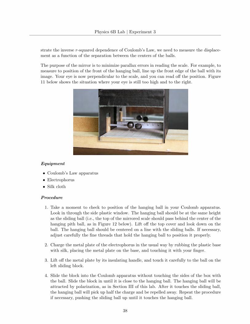
You will be testing the inverse r-squared dependence of Coulomb’s Law with a very simpleapparatus. There is a tall box containing a hanging pith ball covered with a conductingsurface, and similar pith balls on sliding blocks. A mirrored scale permits you to determinethe position of the balls. (The purpose of the closed box is to minimize the effects of aircurrents.)
36
Physics 6B Lab | Experiment 3
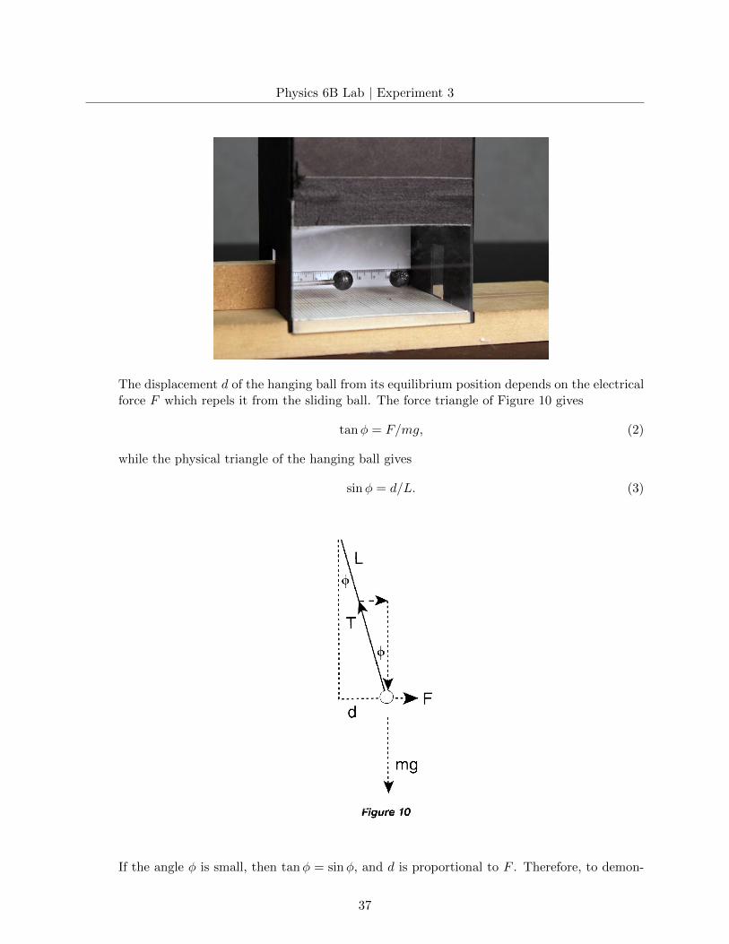
The displacement d of the hanging ball from its equilibrium position depends on the electricalforce F which repels it from the sliding ball. The force triangle of Figure 10 gives
tanφ = F/mg, (2)
while the physical triangle of the hanging ball gives
sinφ = d/L. (3)
If the angle φ is small, then tanφ = sinφ, and d is proportional to F . Therefore, to demon-
37
Physics 6B Lab | Experiment 3
strate the inverse r-squared dependence of Coulomb’s Law, we need to measure the displace-ment as a function of the separation between the centers of the balls.
The purpose of the mirror is to minimize parallax errors in reading the scale. For example, tomeasure to position of the front of the hanging ball, line up the front edge of the ball with itsimage. Your eye is now perpendicular to the scale, and you can read off the position. Figure11 below shows the situation where your eye is still too high and to the right.
Equipment
• Coulomb’s Law apparatus
• Electrophorus
• Silk cloth
Procedure
1. Take a moment to check to position of the hanging ball in your Coulomb apparatus.Look in through the side plastic window. The hanging ball should be at the same heightas the sliding ball (i.e., the top of the mirrored scale should pass behind the center of thehanging pith ball, as in Figure 12 below). Lift off the top cover and look down on theball. The hanging ball should be centered on a line with the sliding balls. If necessary,adjust carefully the fine threads that hold the hanging ball to position it properly.
2. Charge the metal plate of the electrophorus in the usual way by rubbing the plastic basewith silk, placing the metal plate on the base, and touching it with your finger.
3. Lift off the metal plate by its insulating handle, and touch it carefully to the ball on theleft sliding block.
4. Slide the block into the Coulomb apparatus without touching the sides of the box withthe ball. Slide the block in until it is close to the hanging ball. The hanging ball will beattracted by polarization, as in Section III of this lab. After it touches the sliding ball,the hanging ball will pick up half the charge and be repelled away. Repeat the procedureif necessary, pushing the sliding ball up until it touches the hanging ball.
38
Physics 6B Lab | Experiment 3
5. Recharge the sliding ball so it produces the maximum force, and experiment with pushingit toward the hanging ball. The hanging ball should be repelled strongly.
6. You are going to measure the displacement of the hanging ball. You do not need tomeasure the position of its center, but will record the position of its inside edge. Removethe sliding ball and record the equilibrium position of its inside edge that faces thesliding ball, which you will subtract from all the other measurements to determine thedisplacement d.
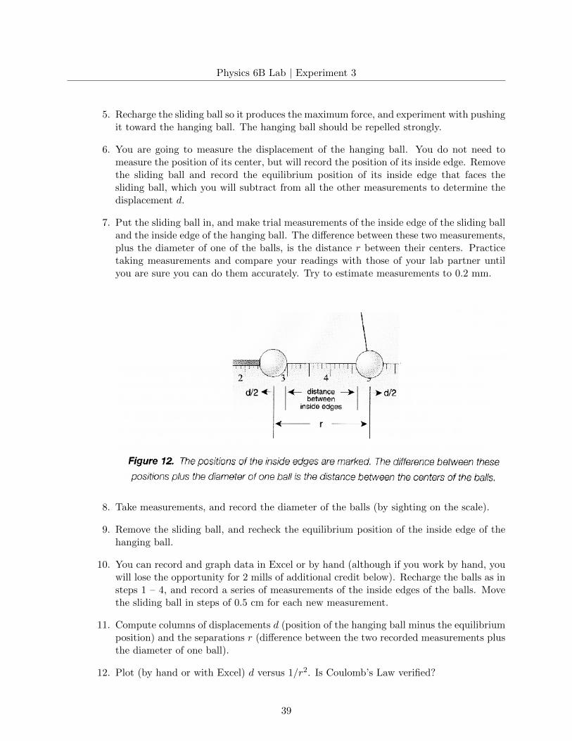
7. Put the sliding ball in, and make trial measurements of the inside edge of the sliding balland the inside edge of the hanging ball. The difference between these two measurements,plus the diameter of one of the balls, is the distance r between their centers. Practicetaking measurements and compare your readings with those of your lab partner untilyou are sure you can do them accurately. Try to estimate measurements to 0.2 mm.
8. Take measurements, and record the diameter of the balls (by sighting on the scale).
9. Remove the sliding ball, and recheck the equilibrium position of the inside edge of thehanging ball.
10. You can record and graph data in Excel or by hand (although if you work by hand, youwill lose the opportunity for 2 mills of additional credit below). Recharge the balls as insteps 1 – 4, and record a series of measurements of the inside edges of the balls. Movethe sliding ball in steps of 0.5 cm for each new measurement.
11. Compute columns of displacements d (position of the hanging ball minus the equilibriumposition) and the separations r (difference between the two recorded measurements plusthe diameter of one ball).
12. Plot (by hand or with Excel) d versus 1/r2. Is Coulomb’s Law verified?
39
Physics 6B Lab | Experiment 3
13. For an additional credit of 2 mills, use Excel to fit a power-law curve to the data. Whatis the exponent of the r-dependence of the force? (Theoretically, it should be −2.000,but what does your curve fit produce?)
14. For your records, you may print out your Excel file with a table and graph of yournumerical observations and any other electronic files you have generated.
ADDITIONAL CREDIT (3 mills)
You can change the charge on the sliding ball by factors of two, by touching it to the other unchargedsliding ball (ground it with your finger first). The balls will share their charge, and half the chargewill remain on the first ball (assuming the balls are the same size). This way, you can obtaincharges on the first ball of Q, Q/2, Q/4, and so forth.
Devise and execute an experiment to verify the dependence of the Coulomb force on the value ofone of the charges. (That is, we want to show that the force is proportional to one of the charges.)The method is up to you; explain your plan and results in your notes. What should you plot againstwhat? Does anything need to be held constant?
40
Physics 6B Lab | Experiment 4
Van de Graaff
APPARATUS
• Heat lamp
• Electroscope
• Lucite rod and silk
• Van de Graaff generator
• Grounding sphere
• Ungrounded sphere
• Faraday cage
• Faraday pail
• Plastic box to stand on
INTRODUCTION
In this experiment, we will continue our study of electrostatics using a Van de Graaff electrostaticgenerator. If the electrostatics experiments were difficult because of humidity during the previousweek, we will intersperse some of them with the experiments this week.
ELECTRIC FIELD
Consider an electric charge exerting forces on other charges which are separated in space from thefirst charge. How can one object exert a force on another object with which it is not in contact?How does the force move across empty space? Does it travel instantaneously at infinite speed orat some finite speed?
In the 19th century, physicists suggested the beginning of a solution to these questions. Instead ofimagining that the charge produces forces on other charges directly, they imagined that the chargefills the surrounding space with an electric field. When other charges are inside the electric field,they experience electrical forces.
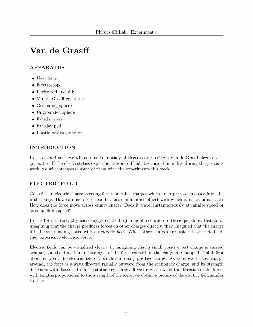
Electric fields can be visualized clearly by imagining that a small positive test charge is carriedaround, and the direction and strength of the force exerted on the charge are mapped. Think firstabout mapping the electric field of a single stationary positive charge. As we move the test chargearound, the force is always directed radially outward from the stationary charge, and its strengthdecreases with distance from the stationary charge. If we draw arrows in the direction of the force,with lengths proportional to the strength of the force, we obtain a picture of the electric field similarto this:
41
Physics 6B Lab | Experiment 4
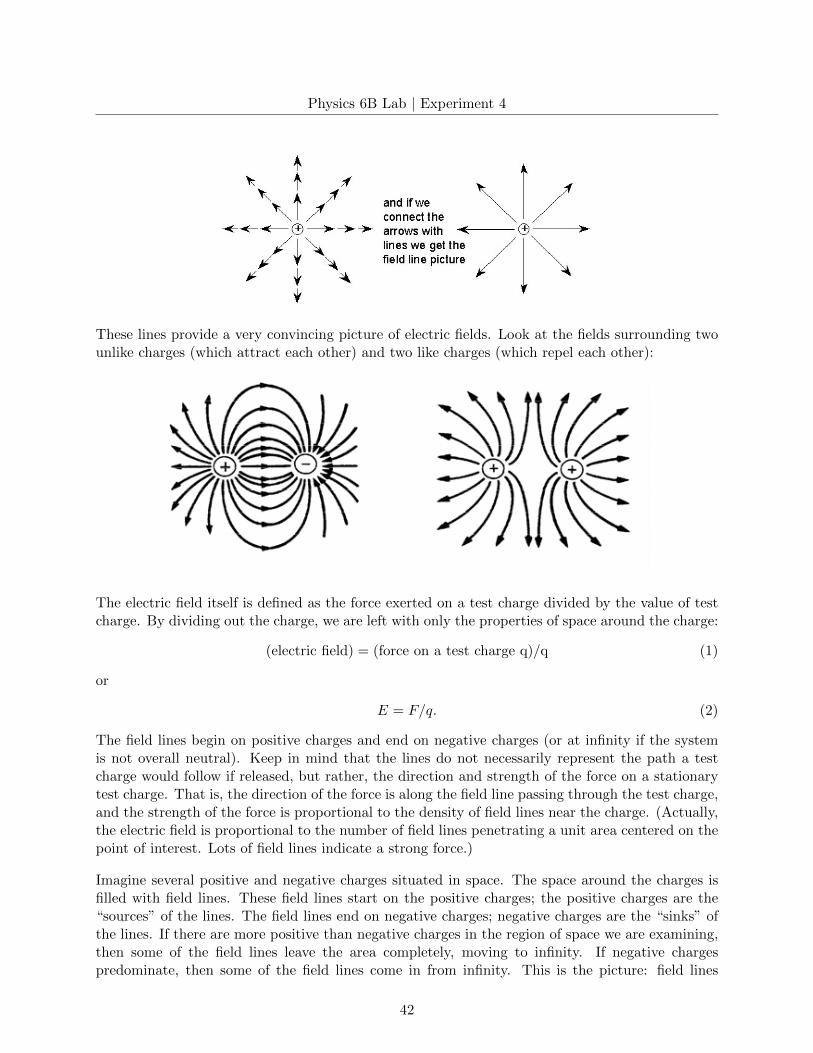
These lines provide a very convincing picture of electric fields. Look at the fields surrounding twounlike charges (which attract each other) and two like charges (which repel each other):
The electric field itself is defined as the force exerted on a test charge divided by the value of testcharge. By dividing out the charge, we are left with only the properties of space around the charge:
(electric field) = (force on a test charge q)/q (1)
or
E = F/q. (2)
The field lines begin on positive charges and end on negative charges (or at infinity if the systemis not overall neutral). Keep in mind that the lines do not necessarily represent the path a testcharge would follow if released, but rather, the direction and strength of the force on a stationarytest charge. That is, the direction of the force is along the field line passing through the test charge,and the strength of the force is proportional to the density of field lines near the charge. (Actually,the electric field is proportional to the number of field lines penetrating a unit area centered on thepoint of interest. Lots of field lines indicate a strong force.)
Imagine several positive and negative charges situated in space. The space around the charges isfilled with field lines. These field lines start on the positive charges; the positive charges are the“sources” of the lines. The field lines end on negative charges; negative charges are the “sinks” ofthe lines. If there are more positive than negative charges in the region of space we are examining,then some of the field lines leave the area completely, moving to infinity. If negative chargespredominate, then some of the field lines come in from infinity. This is the picture: field lines
42
Physics 6B Lab | Experiment 4
filling space, starting on positive charges; or coming in from far away, ending on negative charges;or disappearing into the distance.
The introduction of the electric field concept seems to be an unnecessary complication at first, butphysicists eventually discovered that the equations of electricity and magnetism are simpler whenwritten in terms of fields than in terms of forces. The culmination of this process was reachedaround 1870 with the completion of Maxwell’s equations.
ELECTRIC POTENTIAL
Since an electric field exerts forces on charges in it, there is potential energy associated with theposition of a charged particle in the electric field, just as a massive object has potential energyin the gravitational field of the Earth. Imagine that we hold a positive charge fixed in position,and we bring in a small positive test charge (different from the fixed positive charge) from afar.As we move the positive test charge in, it is repelled by the fixed charge, and we must exert aforce on the test charge to bring it closer. A force exerted though some distance performs work:we must do work on the test charge to move it closer. This work goes into increasing the electricpotential energy of the test charge, just as the work done in lifting an object goes into increasing itsgravitational potential energy. The electric potential energy can be converted into kinetic energyby releasing the test charge. The test charge flies away, gaining kinetic energy in the process.
We would like to introduce a quantity related to potential energy which depends only on theproperties of the charge, so we divide out the test charge and write
(potential) = (potential energy)/(charge) (3)
or
V = U/q. (4)
This relationship defines a new quantity: the electric potential V . Potential is energy per chargeand is measured in joules per coulomb (also known as volts, with unit symbol V). These are thesame volts used in measuring the voltage of a battery. Understanding how the potential energy ofan electric field is related to the voltage of a 6-V battery is one of the difficult conceptual leaps ofelectricity and magnetism. While you are trying to assimilate it, remember that as you learn newconcepts in physics, it is important to keep the basic definitions in mind. If a battery is rated at 6volts, then it is prepared to give 6 joules of energy to every coulomb of charge that is moved fromone of its terminals to the other. For example, if we wire the filament of a small light bulb to thebattery so that charge is moved through the filament, the energy goes into heating the filament“white hot”.
GAUSS’ LAW
Certain results in this lab can be understood most easily on the basis of Gauss’ Law. Gauss’Law is an important reformulation of Coulomb’s Law, which makes easier the derivation of someinteresting consequences of electrostatics, such as the fact that all charge placed on a conductor
43
Physics 6B Lab | Experiment 4
moves to its outside surface. Gauss’ Law can be expressed as a surface integral of the electric field:∫E · dA = qin/ε0. (5)
The surface integral is called the flux of the electric field, and is evaluated over any closed surface.The charge qin is the total charge enclosed within the surface, and ε0 is the constant in Coulomb’sLaw:
F = kqQ/r2 = qQ/4πε0r2 (6)
with k = 1/4πε0.
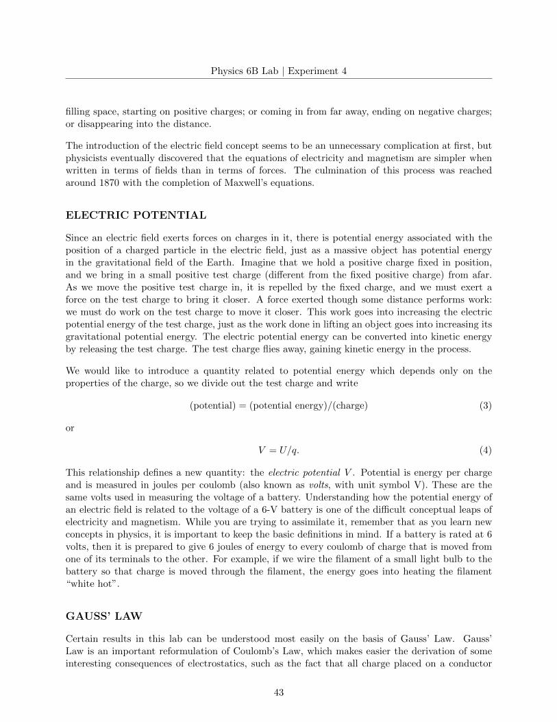
We now derive Coulomb’s Law from Gauss’ Law. Let’s start with an isolated charge q, and drawan imaginary sphere of radius r centered on the charge. This sphere is an example of a Gaussiansurface.
Here the electric field is always perpendicular to the imaginary sphere, and has the same constantvalue E at all points on the surface. Thus, the surface integral is simply the electric field Emultiplied by the surface area 4πr2 of the sphere:∫
E ·dA = E ·∫
dA = E(4πr2) = qin/ε0 = q/ε0. (7)
This gives us the electric field of the charge q at a distance r:
E = q/4πε0r2. (8)
Since the force on a test charge Q due to this electric field is F = QE, we have F = qQ/4πε0r2 —
which is Coulomb’s Law! In this sense, Gauss’ Law is a reformulation of Coulomb’s Law in termsof the electric field. It seems unnecessarily complicated, but you will see that we can immediatelyderive some interesting results with Gauss’ ideas.
You can conceptualize Gauss’ Law in terms of field lines by noting that the integral∫E ·dA over a
surface is proportional to the number of field lines penetrating the surface (regardless of the anglebetween these lines and the surface). If field lines are entering and exiting the surface, then theflux integral is proportional to the number of lines exiting minus the number of field lines entering.
Here is an example. Imagine a closed surface of any shape (a Gaussian surface) enclosing a volumeof space with possibly some charges inside. Let us find the net flux
∫E · dA through this surface.
44
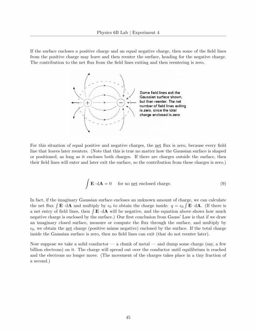
Physics 6B Lab | Experiment 4
If the surface encloses a positive charge and an equal negative charge, then some of the field linesfrom the positive charge may leave and then reenter the surface, heading for the negative charge.The contribution to the net flux from the field lines exiting and then reentering is zero.
For this situation of equal positive and negative charges, the net flux is zero, because every fieldline that leaves later reenters. (Note that this is true no matter how the Gaussian surface is shapedor positioned, as long as it encloses both charges. If there are charges outside the surface, thentheir field lines will enter and later exit the surface, so the contribution from these charges is zero.)
∫E ·dA = 0 for no net enclosed charge. (9)
In fact, if the imaginary Gaussian surface encloses an unknown amount of charge, we can calculatethe net flux
∫E ·dA and multiply by ε0 to obtain the charge inside: q = ε0
∫E · dA. (If there is
a net entry of field lines, then∫E · dA will be negative, and the equation above shows how much
negative charge is enclosed by the surface.) Our first conclusion from Gauss’ Law is that if we drawan imaginary closed surface, measure or compute the flux through the surface, and multiply byε0, we obtain the net charge (positive minus negative) enclosed by the surface. If the total chargeinside the Gaussian surface is zero, then no field lines can exit (that do not reenter later).
Now suppose we take a solid conductor — a chunk of metal — and dump some charge (say, a fewbillion electrons) on it. The charge will spread out over the conductor until equilibrium is reachedand the electrons no longer move. (The movement of the charges takes place in a tiny fraction ofa second.)
45
Physics 6B Lab | Experiment 4
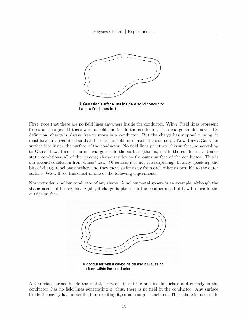
First, note that there are no field lines anywhere inside the conductor. Why? Field lines representforces on charges. If there were a field line inside the conductor, then charge would move. Bydefinition, charge is always free to move in a conductor. But the charge has stopped moving; itmust have arranged itself so that there are no field lines inside the conductor. Now draw a Gaussiansurface just inside the surface of the conductor. No field lines penetrate this surface, so accordingto Gauss’ Law, there is no net charge inside the surface (that is, inside the conductor). Understatic conditions, all of the (excess) charge resides on the outer surface of the conductor. This isour second conclusion from Gauss’ Law. Of course, it is not too surprising. Loosely speaking, thebits of charge repel one another, and they move as far away from each other as possible to the outersurface. We will see this effect in one of the following experiments.
Now consider a hollow conductor of any shape. A hollow metal sphere is an example, although theshape need not be regular. Again, if charge is placed on the conductor, all of it will move to theoutside surface.
A Gaussian surface inside the metal, between its outside and inside surface and entirely in theconductor, has no field lines penetrating it; thus, there is no field in the conductor. Any surfaceinside the cavity has no net field lines exiting it, so no charge is enclosed. Thus, there is no electric
46
Physics 6B Lab | Experiment 4
field inside the cavity. (Strictly speaking, you need another law of electrostatics in addition toGauss’ Law to complete the proof that there is no electric field inside a cavity, devoid of charges,in a conductor. See The Feynman Lectures, Volume II, Section 5 – 10.)
When a volume of space is enclosed by a conductor, there is no static electric field penetrating itfrom the outside. The conductor shields the inner space. This is a very practical example of thestandard advice about remaining inside an automobile during a lightning storm. The automobileencloses its occupants with metal. Even if the automobile is itself struck by lightning and theoccupants are touching its inner surface, the occupants will not be harmed or even shocked. It doesnot matter that the metal surface of the automobile is broken by the non-conducting windows. Asmall electric field may penetrate a short distance at the windows, but the nearly complete metalsurface of the automobile shields the interior very well. A wire mesh cage will effectively shield itsinterior, as long as the mesh hole size in not particularly large compared to the size of the wholecage. We will try a shielding experiment below. Gauss’ Law has other interesting consequences,but we now move to a description of the experimental apparatus.
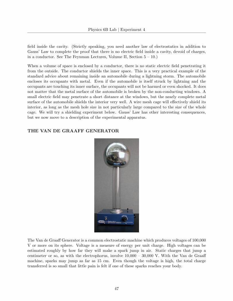
THE VAN DE GRAAFF GENERATOR
The Van de Graaff Generator is a common electrostatic machine which produces voltages of 100,000V or more on its sphere. Voltage is a measure of energy per unit charge. High voltages can beestimated roughly by how far they will make a spark jump in air. Static charges that jump acentimeter or so, as with the electrophorus, involve 10,000 – 30,000 V. With the Van de Graaffmachine, sparks may jump as far as 15 cm. Even though the voltage is high, the total chargetransferred is so small that little pain is felt if one of these sparks reaches your body.
47
Physics 6B Lab | Experiment 4
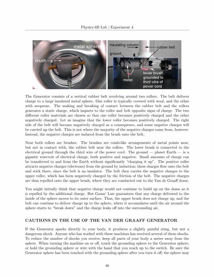
The Generator consists of a vertical rubber belt revolving around two rollers. The belt deliverscharge to a large insulated metal sphere. One roller is typically covered with wool, and the otherwith neoprene. The making and breaking of contact between the rubber belt and the rollersgenerates a static charge, which imparts to the roller and belt opposite signs of charge. The twodifferent roller materials are chosen so that one roller becomes positively charged and the othernegatively charged. Let us imagine that the lower roller becomes positively charged. The rightside of the belt will become negatively charged as a consequence, and some negative charges willbe carried up the belt. This is not where the majority of the negative charges come from, however.Instead, the negative charges are induced from the brush onto the belt.
Near both rollers are brushes. The brushes are comb-like arrangements of metal points near,but not in contact with, the rubber belt near the rollers. The lower brush is connected to theelectrical ground through the third wire of the power cord. The ground — planet Earth — is agigantic reservoir of electrical charge, both positive and negative. Small amounts of charge canbe transferred to and from the Earth without significantly “charging it up”. The positive rollerattracts negative charges (electrons) from the ground by induction; these charges flow onto the beltand stick there, since the belt is an insulator. The belt then carries the negative charges to theupper roller, which has been negatively charged by the friction of the belt. The negative chargesare thus repelled onto the upper brush, where they are conducted out to the Van de Graaff dome.
You might initially think that negative charge would not continue to build up on the dome as itis repelled by the additional charge. But Gauss’ Law guarantees that any charge delivered to theinside of the sphere moves to its outer surface. Thus, the upper brush does not charge up, and thebelt can continue to deliver charge up to the sphere, where it accumulates until the air around thesphere starts to “break down” and the charge leaks off into the surrounding air.
CAUTIONS IN THE USE OF THE VAN DER GRAAFF GENERATOR
If the Generator sparks directly to your body, it produces a slightly painful sting, but not adangerous shock. Anyone who has worked with these machines has received several of these shocks.To reduce the number of shocks you receive, keep all parts of your body a meter away from thesphere. When turning the machine on or off, touch the grounding sphere to the Generator sphere,or hold the grounding sphere or wire with the hand that you reach up to the switch. Be sure theGenerator sphere has been touched with the grounding sphere after you turn it off; the sphere may
48
Physics 6B Lab | Experiment 4
stay charged for many minutes.
On a cold dry day when electrostatics is powerful, charge will actually flow through the air andget on you and any equipment nearby. If you get charged up, sparks will jump from you to theground when you came near various objects. Continually hold a grounding wire to prevent thisfrom happening. You may need to ground carefully the other equipment to prevent spurious resultsin your experiments. On a good day, you are almost certain to receive some small shocks.
EXPERIMENTS
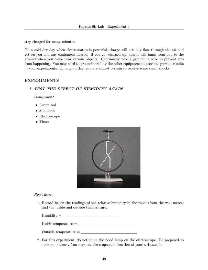
I. TEST THE EFFECT OF HUMIDITY AGAIN
Equipment
• Lucite rod
• Silk cloth
• Electroscope
• Timer
Procedure
1. Record below the readings of the relative humidity in the room (from the wall meter)and the inside and outside temperature.
Humidity =
Inside temperature =
Outside temperature =
2. For this experiment, do not shine the flood lamp on the electroscope. Be prepared tostart your timer. You may use the stopwatch function of your wristwatch.
49

Physics 6B Lab | Experiment 4
3. Rub the lucite rod vigorously with the silk cloth. Use a little whipping motion at the endof the rubbing. Touch the lucite rod to the top of the electroscope. Move the rod alongand around the top so you touch as much of its surface to the metal of the electroscopeas possible. Since the rod is an insulator, charge will not flow from all parts of the rodonto the electroscope; you will need to touch all parts (except where you are holding it)to the electroscope. Start your timer immediately after charging the electroscope.
4. Record the time it takes the electroscope needle to fall completely to 0. Time up tofive minutes, if necessary. If the needle has not fallen to 0 after five minutes, recordan estimate of its angle at the five-minute mark. Typically, after charging, the needlemight be at 80.
II. VAN DE GRAAFF PARAMETERS
The 10-cm spheres on insulating rods are surprisingly expensive and easily dented. Pleasetake care that they do not roll off the table and fall on the floor.
Equipment
• Van de Graaff Generator
• Grounded discharge sphere
• Wire ring with “lightning rod”
• Insulating stand
50
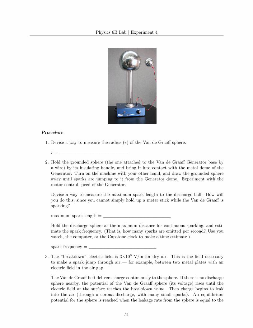
Physics 6B Lab | Experiment 4
Procedure
1. Devise a way to measure the radius (r) of the Van de Graaff sphere.
r =
2. Hold the grounded sphere (the one attached to the Van de Graaff Generator base bya wire) by its insulating handle, and bring it into contact with the metal dome of theGenerator. Turn on the machine with your other hand, and draw the grounded sphereaway until sparks are jumping to it from the Generator dome. Experiment with themotor control speed of the Generator.
Devise a way to measure the maximum spark length to the discharge ball. How willyou do this, since you cannot simply hold up a meter stick while the Van de Graaff issparking?
maximum spark length =
Hold the discharge sphere at the maximum distance for continuous sparking, and esti-mate the spark frequency. (That is, how many sparks are emitted per second? Use youwatch, the computer, or the Capstone clock to make a time estimate.)
spark frequency =
3. The “breakdown” electric field is 3×10⁶ V/m for dry air. This is the field necessaryto make a spark jump through air — for example, between two metal plates with anelectric field in the air gap.
The Van de Graaff belt delivers charge continuously to the sphere. If there is no dischargesphere nearby, the potential of the Van de Graaff sphere (its voltage) rises until theelectric field at the surface reaches the breakdown value. Then charge begins to leakinto the air (through a corona discharge, with many small sparks). An equilibriumpotential for the sphere is reached when the leakage rate from the sphere is equal to the
51
Physics 6B Lab | Experiment 4
delivery rate from the belt.
The electric field E at a distance r from a charged sphere (calculated from Gauss’ Law)is
E = Q/4πε0r2, (10)
where Q is the charge on the sphere. To find the potential V of the sphere, we integrateE from r =∞ to r = R (the radius of the sphere):
V = −∫E dr = Q/4πε0R. (11)
(We suggest, for purposes of midterm preparation in the lecture part of the course, thatyou know how do derive the result above. Getting all the signs correct is somewhattedious.) Using the electric field at the surface of the sphere and eliminating Q, we find
V = ER. (12)
Using E = breakdown electric field, and your measured value of R, calculate the potentialV of the sphere.
V =
Advertisements for this type of Van de Graaff Generator typically state that it willproduce voltages as high as 400,000 V. Is this a reasonable value, taking into accountvarious leakages? What factors might cause the actual potential to be smaller thancalculated?
4. Use your measured maximum spark length and the breakdown electric field to estimatethe potential difference necessary to make a spark jump this distance between two parallelmetal plates.
V =
Is this potential in agreement with your calculated value? How about the advertisedpotential?
5. Using your calculated potential, calculate the charge stored on the sphere from
V = Q/4πε0R. (13)
Express your answer as a number between 1 and 999 in coulombs (C) with the appro-priate prefix, such as m = 10−3, µ = 10−6, n = 10−9, p = 10−12, etc. (It may help toremember that 1/4πε0 = 9× 10⁹ in SI units.)
Q =
6. The capacitance of a configuration of conductors is defined as C = Q/V . The equationabove can be manipulated to give the capacitance of an isolated sphere as
C = 4πε0R. (14)
52
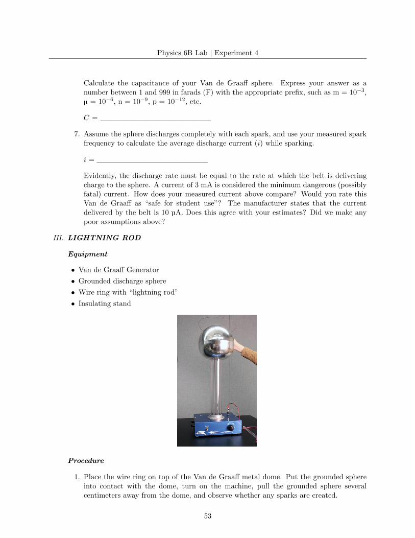
Physics 6B Lab | Experiment 4
Calculate the capacitance of your Van de Graaff sphere. Express your answer as anumber between 1 and 999 in farads (F) with the appropriate prefix, such as m = 10−3,µ = 10−6, n = 10−9, p = 10−12, etc.
C =
7. Assume the sphere discharges completely with each spark, and use your measured sparkfrequency to calculate the average discharge current (i) while sparking.
i =
Evidently, the discharge rate must be equal to the rate at which the belt is deliveringcharge to the sphere. A current of 3 mA is considered the minimum dangerous (possiblyfatal) current. How does your measured current above compare? Would you rate thisVan de Graaff as “safe for student use”? The manufacturer states that the currentdelivered by the belt is 10 µA. Does this agree with your estimates? Did we make anypoor assumptions above?
III. LIGHTNING ROD
Equipment
• Van de Graaff Generator
• Grounded discharge sphere
• Wire ring with “lightning rod”
• Insulating stand
Procedure
1. Place the wire ring on top of the Van de Graaff metal dome. Put the grounded sphereinto contact with the dome, turn on the machine, pull the grounded sphere severalcentimeters away from the dome, and observe whether any sparks are created.
53
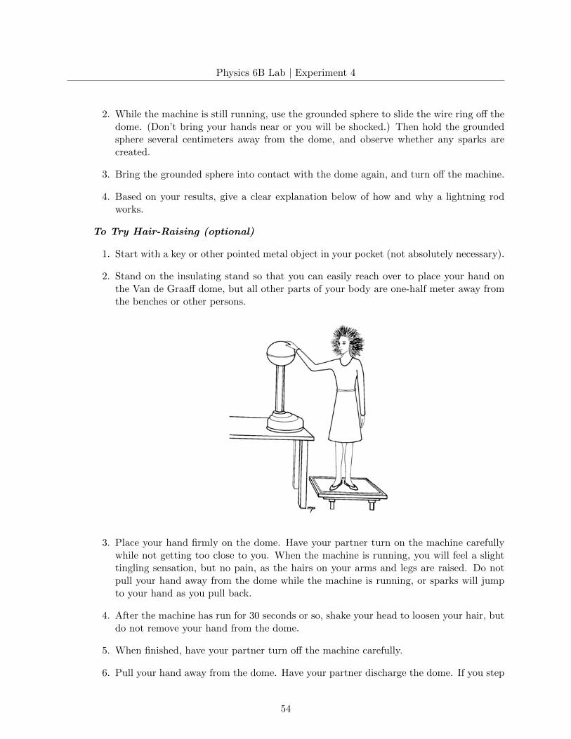
Physics 6B Lab | Experiment 4
2. While the machine is still running, use the grounded sphere to slide the wire ring off thedome. (Don’t bring your hands near or you will be shocked.) Then hold the groundedsphere several centimeters away from the dome, and observe whether any sparks arecreated.
3. Bring the grounded sphere into contact with the dome again, and turn off the machine.
4. Based on your results, give a clear explanation below of how and why a lightning rodworks.
To Try Hair-Raising (optional)
1. Start with a key or other pointed metal object in your pocket (not absolutely necessary).
2. Stand on the insulating stand so that you can easily reach over to place your hand onthe Van de Graaff dome, but all other parts of your body are one-half meter away fromthe benches or other persons.
3. Place your hand firmly on the dome. Have your partner turn on the machine carefullywhile not getting too close to you. When the machine is running, you will feel a slighttingling sensation, but no pain, as the hairs on your arms and legs are raised. Do notpull your hand away from the dome while the machine is running, or sparks will jumpto your hand as you pull back.
4. After the machine has run for 30 seconds or so, shake your head to loosen your hair, butdo not remove your hand from the dome.
5. When finished, have your partner turn off the machine carefully.
6. Pull your hand away from the dome. Have your partner discharge the dome. If you step
54
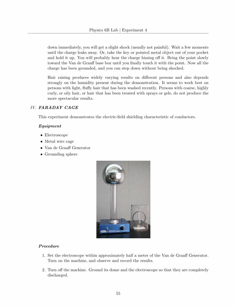
Physics 6B Lab | Experiment 4
down immediately, you will get a slight shock (usually not painful). Wait a few momentsuntil the charge leaks away. Or, take the key or pointed metal object out of your pocketand hold it up. You will probably hear the charge hissing off it. Bring the point slowlytoward the Van de Graaff base box until you finally touch it with the point. Now all thecharge has been grounded, and you can step down without being shocked.
Hair raising produces widely varying results on different persons and also dependsstrongly on the humidity present during the demonstration. It seems to work best onpersons with light, fluffy hair that has been washed recently. Persons with coarse, highlycurly, or oily hair, or hair that has been treated with sprays or gels, do not produce themore spectacular results.
IV. FARADAY CAGE
This experiment demonstrates the electric-field shielding characteristic of conductors.
Equipment
• Electroscope
• Metal wire cage
• Van de Graaff Generator
• Grounding sphere
Procedure
1. Set the electroscope within approximately half a meter of the Van de Graaff Generator.Turn on the machine, and observe and record the results.
2. Turn off the machine. Ground its dome and the electroscope so that they are completelydischarged.
55

Physics 6B Lab | Experiment 4
3. Cover the electroscope with the metal wire cage, and repeat step 1. Try moving the cageeven closer to the dome (with an insulated rod!). Is there any deflection? How do youexplain the results?
V. FARADAY ICE PAIL
In the experiments last week, we have shown that a charged rod can induce an opposite chargeon a conductor. In this section, we will show that the induced charge is not only opposite insign, but also equal in magnitude, to the inducing charge.
Equipment
• Van de Graaff Generator
• Two conducting spheres, one grounded
• Electroscope with Faraday pail
Procedure
1. Position the electroscope with Faraday pail away from the Van de Graaff Generator.(When the metal dome of the Generator is charged, an electroscope nearby may deflectfrom the electric field of the dome, as you found in the last experiment. This deflectionwill end when the dome is discharged. However, on some days charge will actuallymove through the air and get on the electroscope, and the electroscope will remaindeflected even after the dome is discharged. In this case, you will need to discharge theelectroscope with your finger, or perhaps you may need to touch both the top electrode(or pail) and the guard ring of the electroscope with the grounded sphere, to get itcompletely discharged before performing the remaining steps.)
2. Run the Van de Graaff Generator for a few moments until its sphere is charged.
3. Hold the ungrounded conducting sphere by its insulating handle, and charge it by mo-mentarily touching it to the Van de Graaff dome. Discharge the dome. Make sure the
56
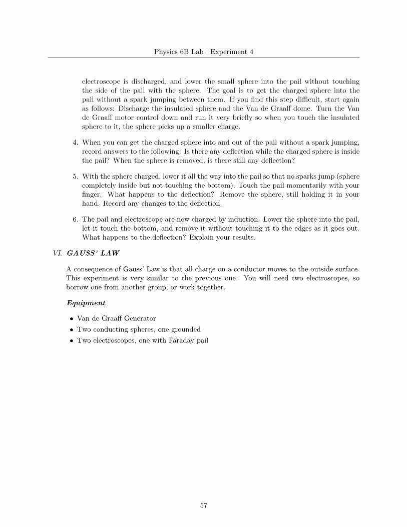
Physics 6B Lab | Experiment 4
electroscope is discharged, and lower the small sphere into the pail without touchingthe side of the pail with the sphere. The goal is to get the charged sphere into thepail without a spark jumping between them. If you find this step difficult, start againas follows: Discharge the insulated sphere and the Van de Graaff dome. Turn the Vande Graaff motor control down and run it very briefly so when you touch the insulatedsphere to it, the sphere picks up a smaller charge.
4. When you can get the charged sphere into and out of the pail without a spark jumping,record answers to the following: Is there any deflection while the charged sphere is insidethe pail? When the sphere is removed, is there still any deflection?
5. With the sphere charged, lower it all the way into the pail so that no sparks jump (spherecompletely inside but not touching the bottom). Touch the pail momentarily with yourfinger. What happens to the deflection? Remove the sphere, still holding it in yourhand. Record any changes to the deflection.
6. The pail and electroscope are now charged by induction. Lower the sphere into the pail,let it touch the bottom, and remove it without touching it to the edges as it goes out.What happens to the deflection? Explain your results.
VI. GAUSS’ LAW
A consequence of Gauss’ Law is that all charge on a conductor moves to the outside surface.This experiment is very similar to the previous one. You will need two electroscopes, soborrow one from another group, or work together.
Equipment
• Van de Graaff Generator
• Two conducting spheres, one grounded
• Two electroscopes, one with Faraday pail
57
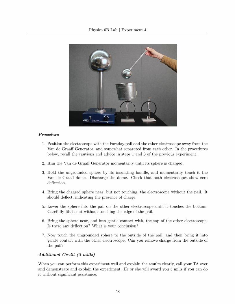
Physics 6B Lab | Experiment 4
Procedure
1. Position the electroscope with the Faraday pail and the other electroscope away from theVan de Graaff Generator, and somewhat separated from each other. In the proceduresbelow, recall the cautions and advice in steps 1 and 3 of the previous experiment.
2. Run the Van de Graaff Generator momentarily until its sphere is charged.
3. Hold the ungrounded sphere by its insulating handle, and momentarily touch it theVan de Graaff dome. Discharge the dome. Check that both electroscopes show zerodeflection.
4. Bring the charged sphere near, but not touching, the electroscope without the pail. Itshould deflect, indicating the presence of charge.
5. Lower the sphere into the pail on the other electroscope until it touches the bottom.Carefully lift it out without touching the edge of the pail.
6. Bring the sphere near, and into gentle contact with, the top of the other electroscope.Is there any deflection? What is your conclusion?
7. Now touch the ungrounded sphere to the outside of the pail, and then bring it intogentle contact with the other electroscope. Can you remove charge from the outside ofthe pail?
Additional Credit (3 mills)
When you can perform this experiment well and explain the results clearly, call your TA overand demonstrate and explain the experiment. He or she will award you 3 mills if you can doit without significant assistance.
58
Physics 6B Lab | Experiment 4
Note: If the previous week was bad for electrostatics, some experiments may be carried overto this week.
59

Physics 6B Lab | Experiment 5
Electrical Circuits
APPARATUS
• Computer and interface
• Voltage sensor
• Fluke 8010A multimeter
• Pasco circuit board with two D-cells
• Box with hook-up leads and components
INTRODUCTION
This experiment is an introduction to the wiring of simple electrical circuits, the use of ammetersand voltmeters, series and parallel circuits, and RC circuits. The circuits will be wired up on thePasco circuit board.
BRIEF REVIEW OF DC CIRCUIT THEORY
In a metal conductor, each atom contributes one or two electrons that can move freely through themetal. An electric current in a wire represents a flow of these electrons. The flow is quite chaoticsince the electrons have a large thermal component to their motion; they are always “jittering”
60
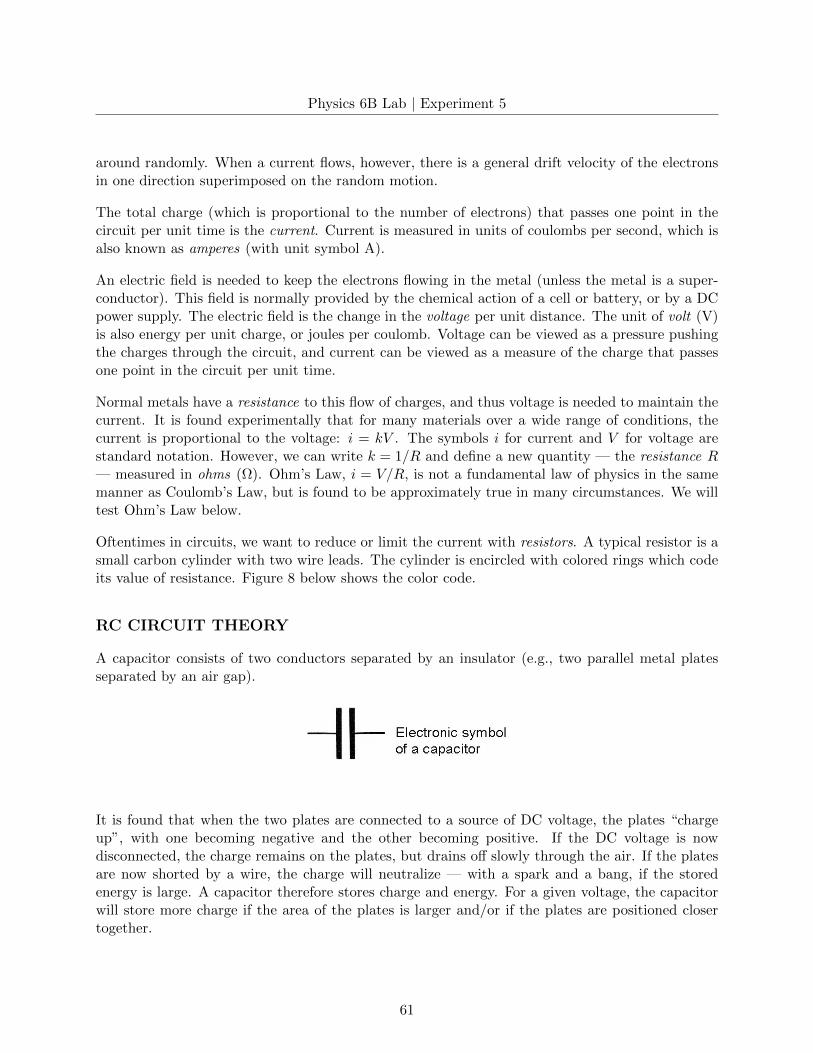
Physics 6B Lab | Experiment 5
around randomly. When a current flows, however, there is a general drift velocity of the electronsin one direction superimposed on the random motion.
The total charge (which is proportional to the number of electrons) that passes one point in thecircuit per unit time is the current. Current is measured in units of coulombs per second, which isalso known as amperes (with unit symbol A).
An electric field is needed to keep the electrons flowing in the metal (unless the metal is a super-conductor). This field is normally provided by the chemical action of a cell or battery, or by a DCpower supply. The electric field is the change in the voltage per unit distance. The unit of volt (V)is also energy per unit charge, or joules per coulomb. Voltage can be viewed as a pressure pushingthe charges through the circuit, and current can be viewed as a measure of the charge that passesone point in the circuit per unit time.
Normal metals have a resistance to this flow of charges, and thus voltage is needed to maintain thecurrent. It is found experimentally that for many materials over a wide range of conditions, thecurrent is proportional to the voltage: i = kV . The symbols i for current and V for voltage arestandard notation. However, we can write k = 1/R and define a new quantity — the resistance R— measured in ohms (Ω). Ohm’s Law, i = V/R, is not a fundamental law of physics in the samemanner as Coulomb’s Law, but is found to be approximately true in many circumstances. We willtest Ohm’s Law below.
Oftentimes in circuits, we want to reduce or limit the current with resistors. A typical resistor is asmall carbon cylinder with two wire leads. The cylinder is encircled with colored rings which codeits value of resistance. Figure 8 below shows the color code.
RC CIRCUIT THEORY
A capacitor consists of two conductors separated by an insulator (e.g., two parallel metal platesseparated by an air gap).
It is found that when the two plates are connected to a source of DC voltage, the plates “chargeup”, with one becoming negative and the other becoming positive. If the DC voltage is nowdisconnected, the charge remains on the plates, but drains off slowly through the air. If the platesare now shorted by a wire, the charge will neutralize — with a spark and a bang, if the storedenergy is large. A capacitor therefore stores charge and energy. For a given voltage, the capacitorwill store more charge if the area of the plates is larger and/or if the plates are positioned closertogether.
61
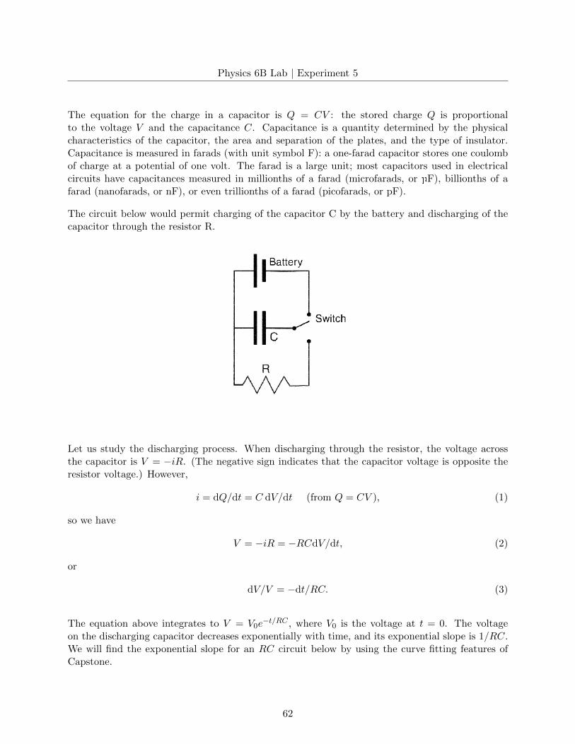
Physics 6B Lab | Experiment 5
The equation for the charge in a capacitor is Q = CV : the stored charge Q is proportionalto the voltage V and the capacitance C. Capacitance is a quantity determined by the physicalcharacteristics of the capacitor, the area and separation of the plates, and the type of insulator.Capacitance is measured in farads (with unit symbol F): a one-farad capacitor stores one coulombof charge at a potential of one volt. The farad is a large unit; most capacitors used in electricalcircuits have capacitances measured in millionths of a farad (microfarads, or µF), billionths of afarad (nanofarads, or nF), or even trillionths of a farad (picofarads, or pF).
The circuit below would permit charging of the capacitor C by the battery and discharging of thecapacitor through the resistor R.
Let us study the discharging process. When discharging through the resistor, the voltage acrossthe capacitor is V = −iR. (The negative sign indicates that the capacitor voltage is opposite theresistor voltage.) However,
i = dQ/dt = C dV/dt (from Q = CV ), (1)
so we have
V = −iR = −RCdV/dt, (2)
or
dV/V = −dt/RC. (3)
The equation above integrates to V = V0e−t/RC , where V0 is the voltage at t = 0. The voltage
on the discharging capacitor decreases exponentially with time, and its exponential slope is 1/RC.We will find the exponential slope for an RC circuit below by using the curve fitting features ofCapstone.
62
Physics 6B Lab | Experiment 5
MULTIMETER
A multimeter is an important tool for anyone working with electrical circuits. A typical multimeterhas different scales and ranges for voltage, current, and resistance. Some multimeters will alsomeasure other quantities such as frequency and capacitance. In this experiment, we will be usingthe Fluke 8010A digital multimeter.
Take a moment to study this instrument. The green push-button power switch is at the lowerright. The left-most button changes the measurements between AC and DC (alternating anddirect current). This button should be out, as all of our measurements for this experiment are inDC.
To measure voltages, press the “V” button, and connect your test leads to the “common” andV/kΩ/S sockets. Push in a button for the appropriate scale: 2 V or 20 V in this experiment. Tomeasure resistances, use the “kΩ” button and an appropriate scale. (Here kΩ represents thousandsof ohms.)
You must be careful when measuring currents. Double-check your circuit when using the currentmeter. The meter must be hooked into the circuit so the current flows through the meter. Thetest leads are connected to the mA (milliampere) and common sockets. Before hooking the meterinto the circuit, estimate first whether you expect the current to exceed 2 A. The meter has a 2-Afuse which will “blow” if this current is exceeded. All of our circuits below use smaller currents,provided they are wired correctly.
HOOKING UP WIRES
Connections are made on the circuit board by pushing a stripped wire or lead to a component intoa spring. For maximum effect, the striped part of the wire should extend in such a way that itpasses completely across the spring, making contact with the spring at four points. This extensionproduces the most secure electrical and mechanical connection.
63
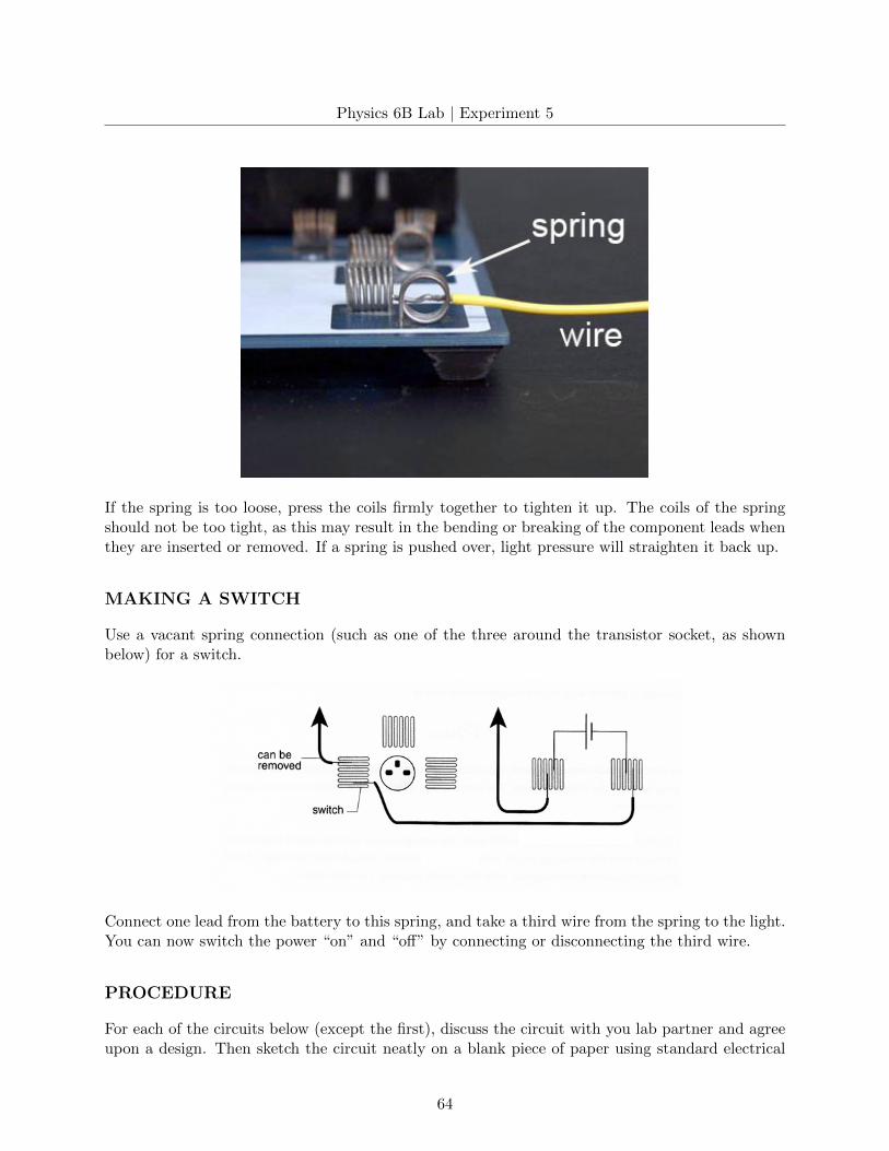
Physics 6B Lab | Experiment 5
If the spring is too loose, press the coils firmly together to tighten it up. The coils of the springshould not be too tight, as this may result in the bending or breaking of the component leads whenthey are inserted or removed. If a spring is pushed over, light pressure will straighten it back up.
MAKING A SWITCH
Use a vacant spring connection (such as one of the three around the transistor socket, as shownbelow) for a switch.
Connect one lead from the battery to this spring, and take a third wire from the spring to the light.You can now switch the power “on” and “off” by connecting or disconnecting the third wire.
PROCEDURE
For each of the circuits below (except the first), discuss the circuit with you lab partner and agreeupon a design. Then sketch the circuit neatly on a blank piece of paper using standard electrical
64
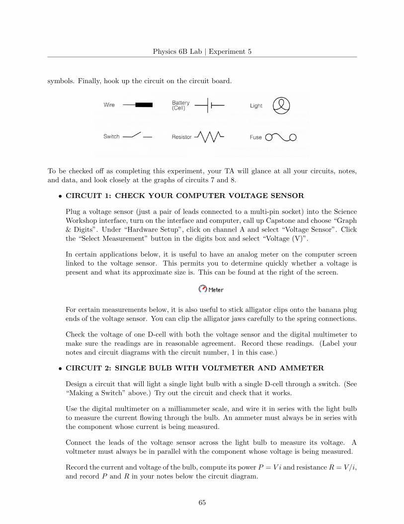
Physics 6B Lab | Experiment 5
symbols. Finally, hook up the circuit on the circuit board.
To be checked off as completing this experiment, your TA will glance at all your circuits, notes,and data, and look closely at the graphs of circuits 7 and 8.
• CIRCUIT 1: CHECK YOUR COMPUTER VOLTAGE SENSOR
Plug a voltage sensor (just a pair of leads connected to a multi-pin socket) into the ScienceWorkshop interface, turn on the interface and computer, call up Capstone and choose “Graph& Digits”. Under “Hardware Setup”, click on channel A and select “Voltage Sensor”. Clickthe “Select Measurement” button in the digits box and select “Voltage (V)”.
In certain applications below, it is useful to have an analog meter on the computer screenlinked to the voltage sensor. This permits you to determine quickly whether a voltage ispresent and what its approximate size is. This can be found at the right of the screen.
For certain measurements below, it is also useful to stick alligator clips onto the banana plugends of the voltage sensor. You can clip the alligator jaws carefully to the spring connections.
Check the voltage of one D-cell with both the voltage sensor and the digital multimeter tomake sure the readings are in reasonable agreement. Record these readings. (Label yournotes and circuit diagrams with the circuit number, 1 in this case.)
• CIRCUIT 2: SINGLE BULB WITH VOLTMETER AND AMMETER
Design a circuit that will light a single light bulb with a single D-cell through a switch. (See“Making a Switch” above.) Try out the circuit and check that it works.
Use the digital multimeter on a milliammeter scale, and wire it in series with the light bulbto measure the current flowing through the bulb. An ammeter must always be in series withthe component whose current is being measured.
Connect the leads of the voltage sensor across the light bulb to measure its voltage. Avoltmeter must always be in parallel with the component whose voltage is being measured.
Record the current and voltage of the bulb, compute its power P = V i and resistance R = V/i,and record P and R in your notes below the circuit diagram.
65
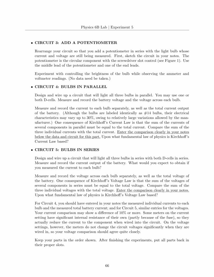
Physics 6B Lab | Experiment 5
• CIRCUIT 3: ADD A POTENTIOMETER
Rearrange your circuit so that you add a potentiometer in series with the light bulb whosecurrent and voltage are still being measured. First, sketch the circuit in your notes. Thepotentiometer is the circular component with the screwdriver slot control (see Figure 1). Usethe middle lead of the potentiometer and one of the end leads.
Experiment with controlling the brightness of the bulb while observing the ammeter andvoltmeter readings. (No data need be taken.)
• CIRCUIT 4: BULBS IN PARALLEL
Design and wire up a circuit that will light all three bulbs in parallel. You may use one orboth D-cells. Measure and record the battery voltage and the voltage across each bulb.
Measure and record the current to each bulb separately, as well as the total current outputof the battery. (Although the bulbs are labeled identically as #14 bulbs, their electricalcharacteristics may vary up to 30%, owing to relatively large variations allowed by the man-ufacturer.) One consequence of Kirchhoff’s Current Law is that the sum of the currents ofseveral components in parallel must be equal to the total current. Compare the sum of thethree individual currents with the total current. Enter the comparison clearly in your notesbelow the data and circuit for this part. Upon what fundamental law of physics is Kirchhoff’sCurrent Law based?
• CIRCUIT 5: BULBS IN SERIES
Design and wire up a circuit that will light all three bulbs in series with both D-cells in series.Measure and record the current output of the battery. What would you expect to obtain ifyou measured the current to each bulb?
Measure and record the voltage across each bulb separately, as well as the total voltage ofthe battery. One consequence of Kirchhoff’s Voltage Law is that the sum of the voltages ofseveral components in series must be equal to the total voltage. Compare the sum of thethree individual voltages with the total voltage. Enter the comparison clearly in your notes.Upon what fundamental law of physics is Kirchhoff’s Voltage Law based?
For Circuit 4, you should have entered in your notes the measured individual currents to eachbulb and the measured total battery current; and for Circuit 5, similar entries for the voltages.Your current comparison may show a difference of 10% or more. Some meters on the currentsetting have significant internal resistance of their own (partly because of the fuse), so theyactually reduce the current to the component when wired into the circuit. On the voltagesettings, however, the meters do not change the circuit voltages significantly when they arewired in, so your voltage comparison should agree quite closely.
Keep your parts in the order shown. After finishing the experiments, put all parts back intheir proper slots.
66
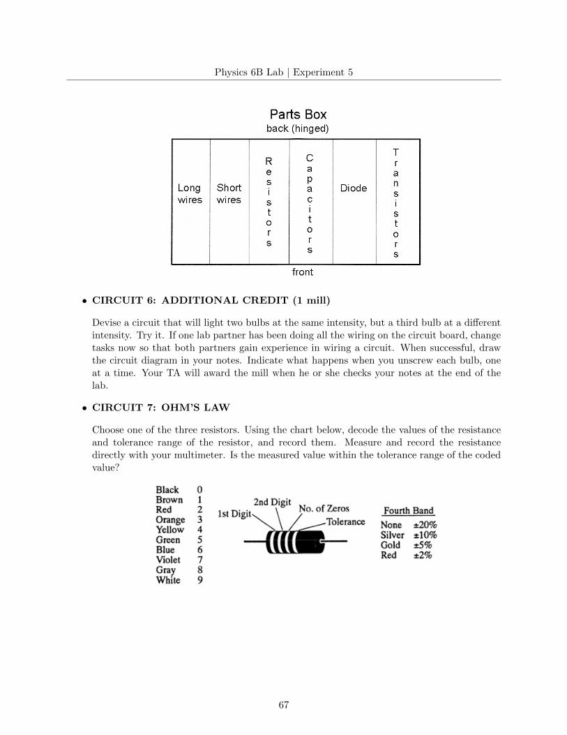
Physics 6B Lab | Experiment 5
• CIRCUIT 6: ADDITIONAL CREDIT (1 mill)
Devise a circuit that will light two bulbs at the same intensity, but a third bulb at a differentintensity. Try it. If one lab partner has been doing all the wiring on the circuit board, changetasks now so that both partners gain experience in wiring a circuit. When successful, drawthe circuit diagram in your notes. Indicate what happens when you unscrew each bulb, oneat a time. Your TA will award the mill when he or she checks your notes at the end of thelab.
• CIRCUIT 7: OHM’S LAW
Choose one of the three resistors. Using the chart below, decode the values of the resistanceand tolerance range of the resistor, and record them. Measure and record the resistancedirectly with your multimeter. Is the measured value within the tolerance range of the codedvalue?
67
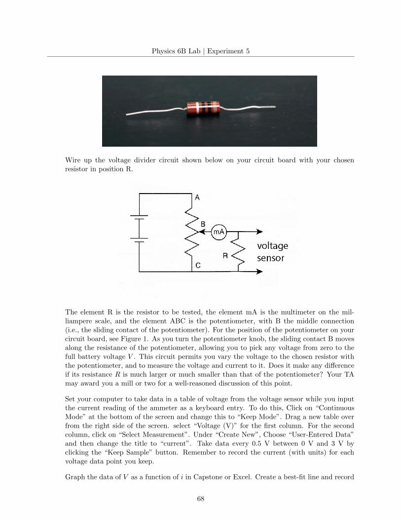
Physics 6B Lab | Experiment 5
Wire up the voltage divider circuit shown below on your circuit board with your chosenresistor in position R.
The element R is the resistor to be tested, the element mA is the multimeter on the mil-liampere scale, and the element ABC is the potentiometer, with B the middle connection(i.e., the sliding contact of the potentiometer). For the position of the potentiometer on yourcircuit board, see Figure 1. As you turn the potentiometer knob, the sliding contact B movesalong the resistance of the potentiometer, allowing you to pick any voltage from zero to thefull battery voltage V . This circuit permits you vary the voltage to the chosen resistor withthe potentiometer, and to measure the voltage and current to it. Does it make any differenceif its resistance R is much larger or much smaller than that of the potentiometer? Your TAmay award you a mill or two for a well-reasoned discussion of this point.
Set your computer to take data in a table of voltage from the voltage sensor while you inputthe current reading of the ammeter as a keyboard entry. To do this, Click on “ContinuousMode” at the bottom of the screen and change this to “Keep Mode”. Drag a new table overfrom the right side of the screen. select “Voltage (V)” for the first column. For the secondcolumn, click on “Select Measurement”. Under “Create New”, Choose “User-Entered Data”and then change the title to “current”. Take data every 0.5 V between 0 V and 3 V byclicking the “Keep Sample” button. Remember to record the current (with units) for eachvoltage data point you keep.
Graph the data of V as a function of i in Capstone or Excel. Create a best-fit line and record
68
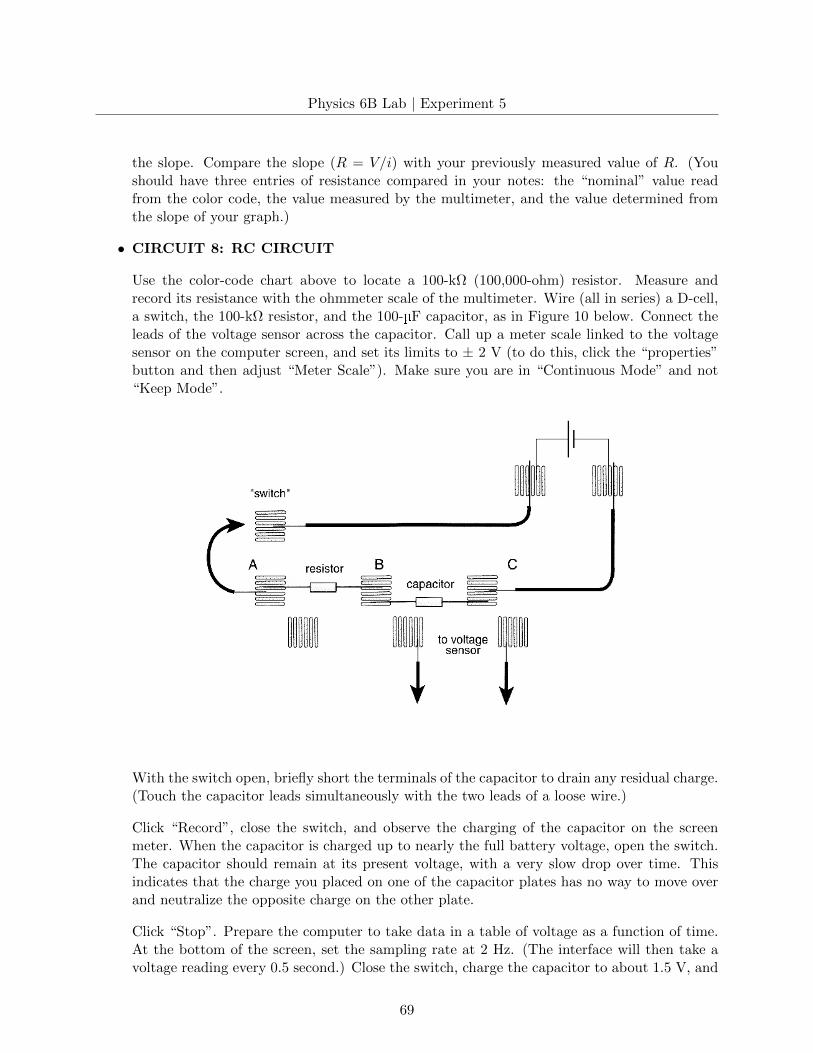
Physics 6B Lab | Experiment 5
the slope. Compare the slope (R = V/i) with your previously measured value of R. (Youshould have three entries of resistance compared in your notes: the “nominal” value readfrom the color code, the value measured by the multimeter, and the value determined fromthe slope of your graph.)
• CIRCUIT 8: RC CIRCUIT
Use the color-code chart above to locate a 100-kΩ (100,000-ohm) resistor. Measure andrecord its resistance with the ohmmeter scale of the multimeter. Wire (all in series) a D-cell,a switch, the 100-kΩ resistor, and the 100-µF capacitor, as in Figure 10 below. Connect theleads of the voltage sensor across the capacitor. Call up a meter scale linked to the voltagesensor on the computer screen, and set its limits to ± 2 V (to do this, click the “properties”button and then adjust “Meter Scale”). Make sure you are in “Continuous Mode” and not“Keep Mode”.
With the switch open, briefly short the terminals of the capacitor to drain any residual charge.(Touch the capacitor leads simultaneously with the two leads of a loose wire.)
Click “Record”, close the switch, and observe the charging of the capacitor on the screenmeter. When the capacitor is charged up to nearly the full battery voltage, open the switch.The capacitor should remain at its present voltage, with a very slow drop over time. Thisindicates that the charge you placed on one of the capacitor plates has no way to move overand neutralize the opposite charge on the other plate.
Click “Stop”. Prepare the computer to take data in a table of voltage as a function of time.At the bottom of the screen, set the sampling rate at 2 Hz. (The interface will then take avoltage reading every 0.5 second.) Close the switch, charge the capacitor to about 1.5 V, and
69
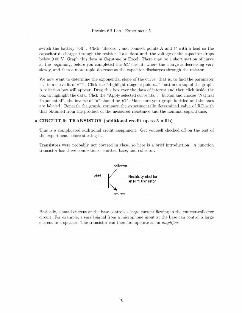
Physics 6B Lab | Experiment 5
switch the battery “off”. Click “Record”, and connect points A and C with a lead so thecapacitor discharges through the resistor. Take data until the voltage of the capacitor dropsbelow 0.05 V. Graph this data in Capstone or Excel. There may be a short section of curveat the beginning, before you completed the RC circuit, where the charge is decreasing veryslowly, and then a more rapid decrease as the capacitor discharges through the resistor.
We now want to determine the exponential slope of the curve: that is, to find the parameter“a” in a curve fit of e−at. Click the “Highlight range of points...” button on top of the graph.A selection box will appear. Drag this box over the data of interest and then click inside thebox to highlight the data. Click the “Apply selected curve fits...” button and choose “NaturalExponential”. the inverse of “a” should be RC. Make sure your graph is titled and the axesare labeled. Beneath the graph, compare the experimentally determined value of RC withthat obtained from the product of the measured resistance and the nominal capacitance.
• CIRCUIT 9: TRANSISTOR (additional credit up to 5 mills)
This is a complicated additional credit assignment. Get yourself checked off on the rest ofthe experiment before starting it.
Transistors were probably not covered in class, so here is a brief introduction. A junctiontransistor has three connections: emitter, base, and collector.
Basically, a small current at the base controls a large current flowing in the emitter-collectorcircuit. For example, a small signal from a microphone input at the base can control a largecurrent to a speaker. The transistor can therefore operate as an amplifier.
70
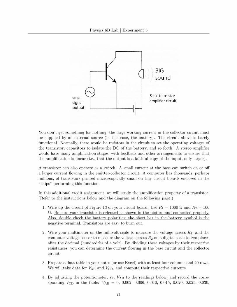
Physics 6B Lab | Experiment 5
You don’t get something for nothing; the large working current in the collector circuit mustbe supplied by an external source (in this case, the battery). The circuit above is barelyfunctional. Normally, there would be resistors in the circuit to set the operating voltages ofthe transistor, capacitors to isolate the DC of the battery, and so forth. A stereo amplifierwould have many amplification stages, with feedback and other arrangements to ensure thatthe amplification is linear (i.e., that the output is a faithful copy of the input, only larger).
A transistor can also operate as a switch. A small current at the base can switch on or offa larger current flowing in the emitter-collector circuit. A computer has thousands, perhapsmillions, of transistors printed microscopically small on tiny circuit boards enclosed in the“chips” performing this function.
In this additional credit assignment, we will study the amplification property of a transistor.(Refer to the instructions below and the diagram on the following page.)
1. Wire up the circuit of Figure 13 on your circuit board. Use R1 = 1000 Ω and R2 = 100Ω. Be sure your transistor is oriented as shown in the picture and connected properly.Also, double check the battery polarities; the short bar in the battery symbol is thenegative terminal. Transistors are easy to burn out.
2. Wire your multimeter on the millivolt scale to measure the voltage across R1, and thecomputer voltage sensor to measure the voltage across R2 on a digital scale to two placesafter the decimal (hundredths of a volt). By dividing these voltages by their respectiveresistances, you can determine the current flowing in the base circuit and the collectorcircuit.
3. Prepare a data table in your notes (or use Excel) with at least four columns and 20 rows.We will take data for VAB and VCD, and compute their respective currents.
4. By adjusting the potentiometer, set VAB to the readings below, and record the corre-sponding VCD in the table: VAB = 0, 0.002, 0.006, 0.010, 0.015, 0.020, 0.025, 0.030,
71
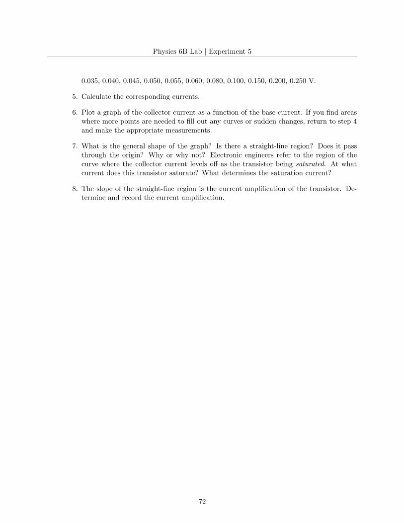
Physics 6B Lab | Experiment 5
0.035, 0.040, 0.045, 0.050, 0.055, 0.060, 0.080, 0.100, 0.150, 0.200, 0.250 V.
5. Calculate the corresponding currents.
6. Plot a graph of the collector current as a function of the base current. If you find areaswhere more points are needed to fill out any curves or sudden changes, return to step 4and make the appropriate measurements.
7. What is the general shape of the graph? Is there a straight-line region? Does it passthrough the origin? Why or why not? Electronic engineers refer to the region of thecurve where the collector current levels off as the transistor being saturated. At whatcurrent does this transistor saturate? What determines the saturation current?
8. The slope of the straight-line region is the current amplification of the transistor. De-termine and record the current amplification.
72
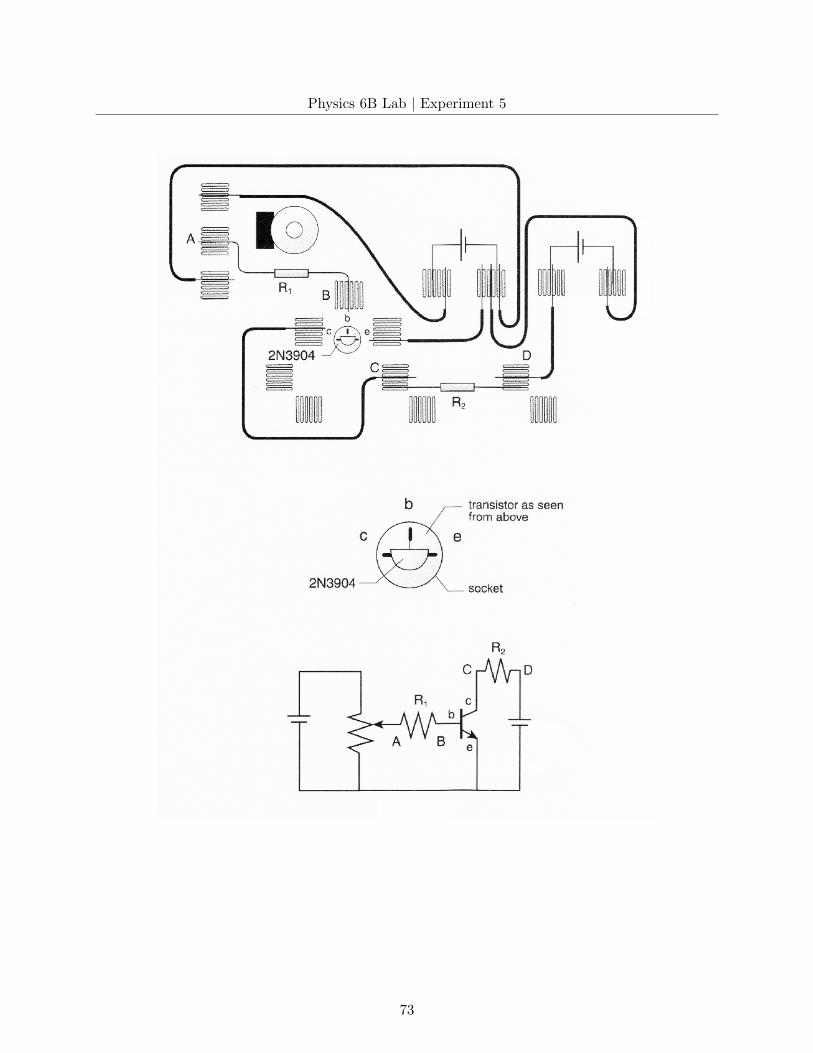
Physics 6B Lab | Experiment 5
73