Copyright

by

Todd Philip Meyrath

2000

TWO-DIMENSIONAL MAGNETO-OPTICAL TRAP

AS A LOW VELOCITY SOURCE OF ATOMIC

SODIUM

by

TODD PHILIP MEYRATH, B.S., B.S.

THESIS

Presented to the Faculty of the Graduate School of

The University of Texas at Austin

in Partial Ful�llment

of the Requirements

for the Degree of

MASTER OF SCIENCE IN APPLIED PHYSICS

THE UNIVERSITY OF TEXAS AT AUSTIN

August 2000

TWO-DIMENSIONAL MAGNETO-OPTICAL TRAP

AS A LOW VELOCITY SOURCE OF ATOMIC

SODIUM

APPROVED BY

SUPERVISING COMMITTEE:

Supervisor:

Mark G. Raizen

Greg O. Sitz

This thesis is dedicated to

Frank William Meyrath Jr.

and

Karen Lynn Meyrath:

my brother and sister,

my best of friends.

Acknowledgments

I would like to thank Prof. Mark Raizen for giving me the opportunity to work

in his research group. Mark is full of ideas, an endless source of knowledge,

and an all-around cool guy | I learned a great deal and had a lot of fun.

Thanks goes to Dr. Valery Milner for working with me on many aspects

of this project and for his helpful discussions and comments. I also appreciate

the suggestions and insights of the senior graduate students Martin Fischer,

Daniel Steck, and Windell Oskay who are always full of knowledge and a

willingness to share. The two semesters I spent as a TA in the senior lab with

Braulio Guti�errez were very educational and interesting, I'd also like to thank

him for interesting discussions and suggestions. Martin and Braulio, thanks

for teaching me to play soccer | maybe someday I will actually be good!

Windell, movie nights were a lot of fun.

Thanks also goes to the other members of the group: Artem Dudarev,

Jay Hanssen, Wes Campbell, and Kevin Henderson. Artem, thanks for all

the Russian phrases. Jay, the courses we had together were interesting | I

will not forget those late nights we spent with Dr. J. D. Jackson. I would

also like to thank former group members Alexander M�uck and Nicole Helbig

for interesting discussions and insights. To all the friends I made in Austin

outside of the research group, especially Adam Clark, Gauri Karve, and Todd

v

Tinsley | you made Austin a unique place. Thanks to everyone for putting

up with my obsessively quoting movies.

I would also like to acknowledge the support given to me by the National

Science Foundation through the NSF Graduate Research Fellowship.

T.P.M.

Austin, Texas

August 16, 2000

vi

TWO-DIMENSIONAL MAGNETO-OPTICAL TRAP

AS A LOW VELOCITY SOURCE OF ATOMIC

SODIUM

Todd Philip Meyrath, M.S.Appl.Phy.The University of Texas at Austin, 2000

Supervisor: Mark G. Raizen

This work describes the design and construction of an experimental apparatus

for a two-dimensional magneto-optical trap (2D-MOT). The 2D-MOT may be

used as a low velocity intense beam source of atomic sodium with application

to load atom traps for novel atom optics experiments. We discuss design

considerations and results obtained.

vii

Table of Contents

Acknowledgments v

Abstract vii

List of Tables x

List of Figures xi

Chapter 1. Background and Inspiration 1

1.1 Introduction . . . . . . . . . . . . . . . . . . . . . . . . . . . . . . 1

1.2 Doppler Cooling . . . . . . . . . . . . . . . . . . . . . . . . . . . . 3

1.2.1 Scattering Force . . . . . . . . . . . . . . . . . . . . . . . . 3

1.2.2 Optical Molasses in 1-D . . . . . . . . . . . . . . . . . . . . 3

1.2.3 Doppler Limit . . . . . . . . . . . . . . . . . . . . . . . . . 5

1.3 A Simple Picture of the Magneto-Optical Trap . . . . . . . . . . . 5

1.3.1 1D-MOT . . . . . . . . . . . . . . . . . . . . . . . . . . . . 5

1.3.2 Standard 3D-MOT . . . . . . . . . . . . . . . . . . . . . . . 8

1.4 Polarization Gradient Cooling . . . . . . . . . . . . . . . . . . . . 9

1.4.1 Polarization Gradient �eld: Linear ? Linear . . . . . . . . . 9

1.4.2 Sisyphus Cooling . . . . . . . . . . . . . . . . . . . . . . . . 10

1.4.3 Polarization Gradient �eld: �+ � �� . . . . . . . . . . . . . 11

1.4.4 �+ � �� Polarization Gradient Cooling . . . . . . . . . . . 12

1.5 Low Velocity Intense Source of Atoms . . . . . . . . . . . . . . . . 13

1.5.1 2D-MOT . . . . . . . . . . . . . . . . . . . . . . . . . . . . 13

1.5.2 LVIS . . . . . . . . . . . . . . . . . . . . . . . . . . . . . . 15

1.5.3 2D+-MOT . . . . . . . . . . . . . . . . . . . . . . . . . . . 15

1.6 Sodium . . . . . . . . . . . . . . . . . . . . . . . . . . . . . . . . . 17

1.6.1 Very Brief History and General Properties . . . . . . . . . . 17

1.6.2 Structure of Sodium . . . . . . . . . . . . . . . . . . . . . . 18

viii

Chapter 2. Experimental Design 22

2.1 Chamber Design . . . . . . . . . . . . . . . . . . . . . . . . . . . . 23

2.1.1 The Idea . . . . . . . . . . . . . . . . . . . . . . . . . . . . 23

2.1.2 The Mirror and Glass Cell . . . . . . . . . . . . . . . . . . 23

2.1.3 Vacuum Chamber Setup . . . . . . . . . . . . . . . . . . . . 27

2.1.4 Chamber Bake . . . . . . . . . . . . . . . . . . . . . . . . . 29

2.2 Io�e Fields . . . . . . . . . . . . . . . . . . . . . . . . . . . . . . . 30

2.2.1 Field of an In�nite Line Current . . . . . . . . . . . . . . . 30

2.2.2 Simple Calculations on Ideal Io�e Con�guration . . . . . . 31

2.2.3 Io�e Coils . . . . . . . . . . . . . . . . . . . . . . . . . . . . 34

2.2.4 Field Measurements . . . . . . . . . . . . . . . . . . . . . . 36

2.3 Current Control Electronics . . . . . . . . . . . . . . . . . . . . . 39

2.3.1 Power Circuit . . . . . . . . . . . . . . . . . . . . . . . . . 40

2.3.2 Control Circuit . . . . . . . . . . . . . . . . . . . . . . . . . 42

2.4 Optical Setup . . . . . . . . . . . . . . . . . . . . . . . . . . . . . 45

2.4.1 Large Elliptical Beam Concerns . . . . . . . . . . . . . . . . 45

2.4.2 Laser and Practical Table Setup Concerns . . . . . . . . . . 46

2.4.3 Optical Setup . . . . . . . . . . . . . . . . . . . . . . . . . 46

Chapter 3. Detection, Observations, Conclusions 51

3.1 Detection Estimates . . . . . . . . . . . . . . . . . . . . . . . . . . 51

3.2 Lock-in Ampli�ers . . . . . . . . . . . . . . . . . . . . . . . . . . . 52

3.3 Plug and Probe Beams and Time-of-Flight . . . . . . . . . . . . . 53

3.4 Summary and Conclusions . . . . . . . . . . . . . . . . . . . . . . 55

Appendix 57

Appendix A. Vacuum Pumps and Gauges 58

Appendix B. Control Circuit Board Layouts 60

Bibliography 63

Vita 66

ix

List of Tables

1.1 General properties of sodium [10, 11]. . . . . . . . . . . . . . . 17

1.2 Characteristics of sodium 32S1=2 � 32P3=2 transition [5, 10, 11]. 19

x

List of Figures

1.1 Counter propagating �+ and �� laser beams detuned from atomicresonance by Ælaser = !atom�!laser are shown. The atomic levelsare shifted due to the Zeeman e�ect in a linear magnetic �eld.The e�ective detuning for a stationary atom at position z0 isÆ� = Ælaser � ge�BGmz

0=~ as in Equations (1.9) and (1.10). . . 6

1.2 3D-MOT pictorial. The large red arrows represent laser beams,the gold loops represent the current loops for creating the �eldsand the blue sphere in the center represents the trapped atoms.Drawing by Windell Oskay. . . . . . . . . . . . . . . . . . . . 8

1.3 Polarization gradient in Linear ? Linear con�guration. Thepolarization changes between circular and linear periodically.Drawing by Alexander M�uck [9]. . . . . . . . . . . . . . . . . 9

1.4 Position dependence of the light shifts of the ground-state sub-levels and optical pumping. Based on a drawing by AlexanderM�uck [9]. . . . . . . . . . . . . . . . . . . . . . . . . . . . . . . 11

1.5 Polarization gradient in �+��� con�guration. The polarizationis linear and rotates in space. Drawing by Alexander M�uck [9]. 12

1.6 2D-MOT pictorial. The Io�e coils produce a linear magnetic�eld gradient in two dimensions. The axis of zero �eld is theatomic beam axis. Atomic velocity along this axis is preserved.Drawing by Todd Meyrath with Windell Oskay. . . . . . . . . 14

1.7 2D+-MOT pictorial of the Diekmann et al. setup. The Io�ecoils produce a linear magnetic �eld gradient in two dimensions.The axis of zero �eld is the atomic beam axis. Beam passesthrough the hole in an aluminum mirror. Drawing by ToddMeyrath with Windell Oskay. . . . . . . . . . . . . . . . . . . 16

1.8 Sodium vapor pressure as a function of temperature [10]. . . . 18

1.9 Sodium structure for the D2 line. The stretched state transition(solid line and dotted line) and the repump (dashed line) areshown. . . . . . . . . . . . . . . . . . . . . . . . . . . . . . . . 20

xi

2.1 A pictorial of our chamber in operation. This is very similar tothat of Dieckmann et al. as pictured in Figure 1.7. On the rightis the `LVIS mirror'. The four elliptical beams enter the sidesof the glass cell (not shown) and the smaller circular beam (onthe left) enter the end of the cell. Drawing by Todd Meyrathwith Windell Oskay. . . . . . . . . . . . . . . . . . . . . . . . 22

2.2 The LVIS mirror. The LVIS mirror is a Zerodur ceramic glasselliptical mirror blank that has been core-drilled and coatedwith a laser line dielectric coating at 589 nm. The hole at themirror surface is elliptical with 0:05 inch minor axis. The mirrorblank was cut out of a Zerodur rod at 45o. . . . . . . . . . . . 24

2.3 Aluminum mount that holds the elliptical mirror inside thechamber. The mirror is shown in place on the right. The el-liptical mirror rests on the lower lip and is pushed by two steelset screws. Near the top of the mirror, three tungsten springspush the mirror against another steel screw that is at 45o to thevertical (i.e., parallel to the surface of the mirror). This holdsthe mirror �rmly in place and provides expansion room duringthe bake to ensure that the glass mirror substrate is not crackedby the screws or holder. . . . . . . . . . . . . . . . . . . . . . 26

2.4 Chamber setup: a) side view: The glass cell is on the left. Thepinch-o� tube (a) contains the sodium. b) top view: The pinch-o� tube (b) was used as the pump out port during bake out. . 28

2.5 The ideal Io�e con�guration consists of four in�nite equal linecurrents represented by the large arrows. . . . . . . . . . . . . 30

2.6 A vector �eld plot of BIo�e in the region between the four wiresas in Equation (2.3). . . . . . . . . . . . . . . . . . . . . . . . 31

2.7 Contour plot of �eld magnitude in the region between the fourwires as in Equation (2.4). . . . . . . . . . . . . . . . . . . . . 32

2.8 Side view of the assembled coil holders (note: assembly looksthe same when looking normal to all four coils). The assembledcoil holder consist of four racetrack shaped Delrin coils that aremounted on a circular aluminum holder that is then mountedto the vacuum chamber. . . . . . . . . . . . . . . . . . . . . . 34

2.9 Photo of the coils in the setup. In the center one can see theglass cell surrounded by the black Delrin racetrack shaped Io�ecoils. They are wrapped with red magnetic wire. The coilassembly ends with a Delrin retaining ring for stability. Aboveand to the sides of the the coil assembly one can see the 3inch lenses that are the objectives for the four large telescopesdiscussed in Section 2.4.1. . . . . . . . . . . . . . . . . . . . . 35

xii

2.10 Measured magnetic �eld near center zero �eld line. This mea-surement was done in the x direction where the y and z com-ponents are zero. The dashed line is for current I = 0:5Ain all coils. The solid line is for current I = 0:8A in allcoils. The crosses mark the data points which have error lessthen �0:01G. It is noted that the sets of data form straightlines as expected from theory. The magnetic �eld gradients areGm(I = 0:5A) = 6:75G=cm and Gm(I = 0:8A) = 10:4G=cm,respectively. . . . . . . . . . . . . . . . . . . . . . . . . . . . . 37

2.11 This plot shows the change in the zero position of the magnetic�eld in the x direction for a change of current in coil 1. Coils 2 to4 have current I = 0:5A. The dotted line is for measured valuesand the solid line is theory (Equation (2.10) with d = 69:5mmand I0 = 0:5A). . . . . . . . . . . . . . . . . . . . . . . . . . . 38

2.12 This plot shows the change in the zero position of the magnetic�eld in the x direction for a change of current in coil 1. Coils 2 to4 have current I = 0:8A. The dotted line is for measured valuesand the solid line is theory (Equation (2.10) with d = 69:5mmand I0 = 0:8A). . . . . . . . . . . . . . . . . . . . . . . . . . . 39

2.13 Power circuit. Current is controlled by the FET, the \snubber"part of the circuit is to limit the inductive kick and provide afast shuto� of the �eld. . . . . . . . . . . . . . . . . . . . . . . 41

2.14 Current control circuit (based on design by Martin Fischer).Feedback loop with the power circuit controls the current inthe coil. . . . . . . . . . . . . . . . . . . . . . . . . . . . . . . 43

2.15 Simpli�ed general example of the control circuit operation. . . 44

2.16 Stable voltage reference for control circuit in Figure 2.14. TheLM399 package is a temperature stabilized zener diode whichserves as the reference voltage of about 7V. . . . . . . . . . . 44

2.17 Optics setup. See Section 2.4.3 for discussion. . . . . . . . . . 49

2.18 Photo of optical setup. This is a photograph of the experimentat some mid-point of the setup. . . . . . . . . . . . . . . . . . 50

3.1 Lock-in ampli�er block diagram. . . . . . . . . . . . . . . . . . 52

3.2 Time-of- ight measurement method to determine atom beamvelocity distribution. The plug beam is modulated by the AOMand the modulation signal is locked-in with the uorescence signal. 54

B.1 Photo of the electronics box. Near the front panel are fourcontrol circuit boards. On the large heat sinks in the rear ofthe box are the power circuits. . . . . . . . . . . . . . . . . . . 60

xiii

B.2 Control circuit board layout (done in EAGLE by Todd Meyrath).This board has both the control circuit of Figure 2.14 and thevoltage reference circuit as in Figure 2.16. . . . . . . . . . . . 61

B.3 Circuit for the panel LCD. . . . . . . . . . . . . . . . . . . . . 62

B.4 Circuit board layout for the LCD (done in EAGLE by ToddMeyrath). This board serves the simple purpose of supplyingthe correct supply voltage to the LCD package from the voltagerails in the box. It is mounted on the LCD on the front panel. 62

xiv

Chapter 1

Background and Inspiration

1.1 Introduction

Generation of intense, slow atomic beams is of great interest to experiments in

ultra-cold atomic physics. Such a beam may be used to load a magneto-optical

trap (MOT) and a magnetic trap for evaporative cooling. One widely used

method of generating slow atomic beams is the so-called Zeeman slower. In

that system, the hot output of an oven is slowed by a cooling laser together

with a tapered magnetic �eld produced by a solenoid. The Zeeman slower,

however, has the undesirable property of being very bulky | a convenient

and compact apparatus is preferred. Recent techniques for generating slow

atomic beams involving vapor-cell MOTs have been explored by several groups

[1, 2, 3]. These methods can provide atomic beams that are near the MOT

capture velocity (of order 10m=s) without the bulk of a Zeeman slower.

This thesis describes the design and construction of an experimental

apparatus for a two-dimensional magneto-optical trap (2D-MOT).We begin by

giving a simple picture of the basic physics relevant to this project. In Section

1.2 there is a discussion of the basics of Doppler cooling and its limits. Doppler

cooling uses spontaneous forces to dampen atomic motion (so-called optical

1

2

molasses). Section 1.3 extends this picture to a MOT where spontaneous forces

are used to trap atoms. This is followed, in Section 1.4, by a discussion of some

of the mechanisms by which atoms may be cooled below the limit of Doppler

cooling. These mechanisms are due to the spatially changing polarization of

the light �eld (polarization gradient cooling).

The essential idea of this project is to use an extension of a 2D-MOT

con�guration (a 2D+-MOT) to produce a cold atomic beam. The idea is

discussed in some detail in Section 1.5.

In Chapter 2, we discuss the design and construction of di�erent aspects

of the experiment. The vacuum chamber is where the physics takes place. We

discuss its components in Section 2.1. Another important aspect of the 2D-

MOT is the magnetic �eld. A set of Io�e coils were constructed to produce

a �eld with a linear gradient in two dimensions and no gradient in the other.

This geometry is an important part of the setup. The design of the coils

and measurements of the �eld produced are in Section 2.2. This discussion is

followed by a description of the current control electronics in Section 2.3 and

optical setup in Section 2.4.

3

1.2 Doppler Cooling

1.2.1 Scattering Force

Consider the absorption process of a photon by a two level atom in the ground

state. After the event, the internal state of the atom has changed to the excited

state and the momentum of the photon is absorbed as a recoil which modi�es

the atom's velocity. The internally excited atom may then undergo sponta-

neous emission which also produces a recoil of the atom. Since spontaneous

emission is equally likely in opposite directions, the recoil of a large number

of spontaneous emission events averages to zero. We will call this absorption-

spontaneous emission process a scattering event. The average force an atom

feels due to a large number of such events is

Fsp = R~k; (1.1)

where R is the rate of scattering. This rate is given by [4]

R =I =2Is

1 + I=Is + (2Æ= )2; (1.2)

where is the rate of decay of the excited state, I is the laser intensity,

Is = �hc=3�3� is the saturation intensity (see Table 1.2 for sodium numbers),

and Æ = !light � !atom is the detuning from atomic resonance.

1.2.2 Optical Molasses in 1-D

Now suppose we have a pair of counterpropagating laser beams of intensity I

and frequency !laser. The laser detuning is de�ned as

Ælaser = !laser � !atom; (1.3)

4

for which the laser is said to be red-detuned or blue-detuned for negative or

positive values, respectively. More generally, since the atoms are moving, we

consider an e�ective detuning of

Æ� = Ælaser � kv; (1.4)

where the second term on the right is due to the Doppler e�ect. The total

scattering force on an atom in this light �eld is the sum of the forces from each

laser: F = F+ + F�. This can be written out as

F (v) =1

2~k

I

Is

�1

1 + I=Is + (2Æ+= )2�

1

1 + I=Is + (2�= )2

�: (1.5)

Suppose the lasers are red-detuned (Ælaser is negative). In this case,

we see that when an atom is moving towards the source of one of the laser

beams it is closer to resonance with that beam and farther from resonance

with the other beam. The atom, therefore, scatters more photons traveling in

the direction opposite to atomic motion and is slowed down. We can consider

this more explicitly in the small velocity limit v � Ælaser=k. Equation (1.5) can

be expanded to �rst order in v:

F (v) =4~k(I=Is)(2Ælaser= )

[1 + I=Is + (2Ælaser= )2]2kv: (1.6)

Since the laser is red-detuned, Equation (1.6) describes a damping force:

F (v) = ��v: (1.7)

With this in mind, we see that atomic motion in this laser �eld obeys the

di�erential equation for particle motion in a viscous uid. Hence, the name

optical molasses is used [5, 6].

5

1.2.3 Doppler Limit

If Equation (1.6) completely described the system, then the atomic velocity

would become arbitrarily close to zero given suÆcient time. In this case, the

ultimate temperature would be T = 0. However, this is not the case.

As noted in Section 1.2.1, the average change in momentum of an atom

involved in a large number of spontaneous emission events in zero. However,

the rms change is non-zero. One might visualize this as a random walk in

momentum space, where the step size is that of the photon momentum ~k

with step frequency 2 . From the theory of Brownian motion, the steady-

state temperature is found to be

TD =~

2kB: (1.8)

This temperature is called the Doppler cooling limit (see Table 1.2 for sodium

numbers) [5, 6].

1.3 A Simple Picture of the Magneto-Optical Trap

1.3.1 1D-MOT

Now, consider the situation of a two level atom with Me = �1; 0;+1 excited

state Zeeman levels in a linear magnetic �eld given by:

B = Gmz; (1.9)

where Gm is the magnetic �eld gradient in gauss=centimeter. Suppose that we

have a pair of counterpropagating circularly polarized laser beams of opposite

helicity detuned by Ælaser = !laser � !atom as in Figure 1.1. The �+ light

6

z

Me = �1

Me = 0

Me = +1 Me = �1

Me = 0

Me = +1

Mg = 0

E

Ælaser

�

Æ+

z0

!laser

!atom

�+ ��

Figure 1.1: Counter propagating �+ and �� laser beams detuned from atomicresonance by Ælaser = !atom � !laser are shown. The atomic levels are shifted

due to the Zeeman e�ect in a linear magnetic �eld. The e�ective detuning fora stationary atom at position z0 is Æ� = Ælaser � ge�BGmz

0=~ as in Equations

(1.9) and (1.10).

couples to the Mg = 0 �! Me = +1 transition and the �� light to the

Mg = 0 �!Me = �1. The e�ective detuning, as in Equation (1.2), is

Æ� = Ælaser � kv � (geMe � ggMg)�BB=~; (1.10)

in general, where Mg and Me are Zeeman sub-levels of the ground and excited

states, and gg and ge are corresponding Land�e g-factors. The second term on

the right of Equation (1.10) is due to the Doppler e�ect and the third to the

Zeeman e�ect. In the case of this simple example, of course, the Mg term on

the right does not appear since Mg = 0.

7

The force that an atom feels in this situation is also described by Equa-

tion (1.5) but now with � as de�ned in Equation (1.10) rather than Equation

(1.4). This adds position dependence to F (in addition to velocity depen-

dence):

F (z; v) =1

2~k

I

Is

�1

1 + I=Is + (2Æ+= )2�

1

1 + I=Is + (2�= )2

�: (1.11)

In the small velocity and weak �eld limit, i.e. where v � Ælaser=k and B �

~Ælaser=�B, Equation (1.11) can be expanded:

F (z; v) =4~k(I=Is)(2Ælaser= )

[1 + I=Is + (2Ælaser= )2]2(kv + (ge�BGm=~)z): (1.12)

The equation of motion is therefore:

�z + trap _z + !2trapz = 0; (1.13)

where

trap =4~k2(I=Is)(2(�Ælaser)= )

m [1 + I=Is + (2Ælaser= )2]2 ; (1.14)

!2trap =

4~k(ge�BGm=~)(I=Is)(2(�Ælaser)= )

m [1 + I=Is + (2Ælaser= )2]2

; (1.15)

and m is the atomic mass. In a MOT, the laser detuning Ælaser = !laser�!atom

is red, so Equation (1.13) is that of a damped harmonic oscillator. This motion

can be characterized by

� � 2trap

4!2trap

=~k3(I=I0)(2(�Ælaser)= )

(ge�BGm=~)m [1 + I=Is + (2Ælaser= )2]2: (1.16)

In a typical experimental situation, with Gm � 10G=cm and Ælaser � 20MHz,

� is of order 100 which clearly makes the motion strongly over damped. Any

displacement therefore decays exponentially towards the center.

8

1.3.2 Standard 3D-MOT

One might imagine the concept of the previous section extended to three di-

mensions, as in Figure 1.2. The current carrying coils produce a spherical

quadrupole magnetic �eld. Six mutually perpendicular laser beams propagate

through the center of the trap. The �� and �+ polarizations are oriented so

that the light couples to the down-shifted zeeman level in all directions. This

con�guration was �rst demonstrated by Raab et al. at AT&T Bell Labs in

1987 [7].

Figure 1.2: 3D-MOT pictorial. The large red arrows represent laser beams,the gold loops represent the current loops for creating the �elds and the blue

sphere in the center represents the trapped atoms. Drawing by Windell Oskay.

9

yE

xE σ − σ +1E

2E − 1E

0 λ/8 λ/4 3λ/8 λ/2y

x

z

Figure 1.3: Polarization gradient in Linear ? Linear con�guration. The polar-ization changes between circular and linear periodically. Drawing by Alexander

M�uck [9].

1.4 Polarization Gradient Cooling

Experimental measurements of temperatures below the Doppler limit called for

new models. In particular, we brie y summarize polarization gradient cooling

for Linear ? Linear and �+� �� con�gurations as described by Dalibard and

Cohen-Tannoudji [8]

1.4.1 Polarization Gradient �eld: Linear ? Linear

Consider the situation of a pair of counterpropagating laser beams with per-

pendicular linear polarizations (say "left = x and "right = y). The total �eld is

the sum

E=E0 = x cos(!lasert� kz) + y cos(!lasert+ kz)

= (x+ y) cos(!lasert) cos(kz) + (x� y) sin(!lasert) sin(kz):(1.17)

This �eld is shown in Figure 1.3. The �eld at some locations of interest is

given by:

E(z = 0)=E0 = (x+ y) cos(!lasert) (1.18)

10

corresponding to linear polarization at 45o, similarly at z = �=4 the �eld is

linear at �45o. Another interesting location is at z = �=8; the �eld there is

E(z = �=8)=E0 = x sin(!lasert + �=4)� y cos(!lasert+ �=4): (1.19)

This is circular polarization (��), similarly at z = 3�=8 the �eld is circular

with the opposite helicity (�+) [5].

1.4.2 Sisyphus Cooling

One model for sub-Doppler cooling is that of linear ? linear polarization gra-

dient cooling | so-called Sisyphus cooling (Dalibard and Cohen-Tannoudji

considered a J = 1=2 !3=2 transition, as we will discuss here). The po-

larization gradient �eld as discussed in the previous section has important

e�ects.

In addition to driving level transitions, the interaction of light with an

atom may cause so-called `light shifts'. This can be thought of as a Stark

e�ect, of sorts, with the electric �eld of the light. It is important to note

that these are not the same for various sublevels | di�erent polarizations can

produce very di�erent light shifts. Figure 1.4 shows the position dependence

of the light shifts of the ground-state sublevels. At the location of �� (see

Figure 1.3), optical pumping drives the ground state population towards the

Mg = �1=2 sublevel. For �+, the population is driven towards the Mg = +1=2

sublevel. Looking at Figure 1.4 one can imagine this cooling process. As an

atom moves through space, it climbs the potential hill | that is, kinetic energy

is converted into potential energy. Before sliding down the other side of the

hill, the atom may be optically pumped to the other ground state sublevel. In

11

0 λ/4 λ/2

Ene

rgy

Position

0

M = +

M = -

g

g

12

12

Figure 1.4: Position dependence of the light shifts of the ground-state sublevelsand optical pumping. Based on a drawing by Alexander M�uck [9].

the optical pumping process here, the spontaneously emitted photon is slightly

higher energy then the absorbed photon. So the some of the atom's kinetic

energy is radiated away.

1.4.3 Polarization Gradient �eld: �+ � ��

Now consider counterpropagating laser beams with circular polarization of

opposite helicity (say �+ from the left and �� from the right). The total �eld

12

is the sum

E=E0 = [x cos(!lasert� kz) + y cos(!lasert� kz)]

+ [x cos(!lasert+ kz)� y cos(!lasert + kz)]

= cos(!lasert) [x cos(kz) + y sin(kz)] :

(1.20)

This is a linear polarization that rotates along the z-axis as shown in Figure

1.5.

σ + σ −

yE

z

Figure 1.5: Polarization gradient in �+ � �� con�guration. The polarizationis linear and rotates in space. Drawing by Alexander M�uck [9].

1.4.4 �+ � �� Polarization Gradient Cooling

Another model for sub-Doppler cooling introduced by Dalibard and Cohen-

Tannoudji is for the �+��� con�guration (they assumed Jg = 1). As discussed

in the previous section, the polarization is linear and rotating. Obviously in

the �+ � �� case, Sisyphus cooling is not possible since the polarization is

linear everywhere (i.e., the light shift is uniform). An atom in this �eld sees

a rotating axis of quantization. The population of the ground state must

be optically pumped to follow. This pushes ground population towards the

Mg = +1 sublevel and towards theMg = �1 sublevel when the atom is moving

toward the �+ and the ��, respectively. An atom with population in the

13

Mg = +1 state will scatter �+ light more eÆciently (according to the Clebsch-

Gordan coeÆcients), and vice versa. So an atom moving towards either beam

will experience a damping force. Although it has a similar apparent e�ect to

that of Doppler cooling, this is purely due to di�erential scattering of light,

and not caused by the Doppler shift as discussed in Section 1.2.

1.5 Low Velocity Intense Source of Atoms

The idea of this project is to create a convenient tool to quickly load large

numbers of sodium atoms in a magnetic trap for evaporative cooling to be

used in experiments of fundamental quantum mechanics. Here, we discuss the

various possible con�gurations of such a source; the terminology of Diekmann

et al. is used (e.g. 2D-MOT, LVIS, 2D+-MOT) [1].

1.5.1 2D-MOT

In Section 1.3.1, we described a simple picture of a MOT in one dimension.

One now imagines this extended to two dimensions in the lab. A Io�e coil

con�guration (to be described in Section 2.2), produces a linear �eld gradient

near the center of the trap in x and y and no gradient in z. The magnetic

�eld zero de�nes a natural axis (the z-axis). One might direct red detuned

laser beams of the correct polarization along the x and y-axes. Atoms from

the vapor are then pushed towards the z-axis and cooled, but their velocity

component in the z direction is preserved. Therefore, it is expected such a

con�guration will produce atomic beams in both directions along the axis of

the zero �eld (z-axis). This is shown pictorially in Figure 1.6. In order to

limit the velocity of atoms in an atomic beam, one may put a small aperture

14

Figure 1.6: 2D-MOT pictorial. The Io�e coils produce a linear magnetic �eldgradient in two dimensions. The axis of zero �eld is the atomic beam axis.Atomic velocity along this axis is preserved. Drawing by Todd Meyrath with

Windell Oskay.

for the atomic beam to pass through. Atoms with large velocity components

in the z direction do not spend enough time in the transverse cooling region

to keep them from being �ltered by the aperture downstream. Therefore, the

atomic beam has mean velocity much smaller than that of the background

atoms. Dieckmann et al. did this experiment with an elliptical beam size

of wz = 24mm and w� = 7mm major and minor waists, respectively. The

purpose of the elongated laser beams along the atomic beam axis is to have

as large a trapping region as possible. The results obtained by Dieckmann

et al. for this setup include a signi�cantly larger mean velocity and width of

15

velocity distribution (see Figure 2 in reference [1]) than the LVIS and 2D+-

MOT con�gurations to be described in the next two sections.

1.5.2 LVIS

LVIS is an acronym that stands for Low Velocity Intense Source [2]. Dieck-

mann et al. use `LVIS' to refer to a speci�c type of con�guration (other then

the 2D-MOT or 2D+-MOT), although \Low Velocity Intense Source" should,

in principle, refer to any con�guration that has such characteristics (such as

the 2D-MOT or 2D+-MOT). Instead of the Io�e con�guration of the 2D-MOT,

the LVIS is similar to a standard MOT with the anti-Helmholtz coil con�gu-

ration (as in Figure 1.2). It di�ers by having a shadow region in one beam. A

common experimental setup involves retrore ecting the beams | one group

designing an LVIS used a gold coated quarter wave plate with a small drilled

hole as a retrore ecter [3]. The quarter wave plate is for the polarization and

the coating for re ection, i.e. the beam passes through the quarter wave plate

before and after re ecting from the back side. Diekmann et al. used an alu-

minum mirror at 45o with a small hole drilled in it as a re ector of a separately

controlled beam. In the LVIS con�guration, atoms experience unbalanced ra-

diation pressure and escape as an atomic beam through the hole.

1.5.3 2D+-MOT

Diekmann et al. performed three experiments in the same apparatus, the third

of which they called the 2D+-MOT. This design might be considered similar

to both the 2D-MOT and LVIS of the previous sections. The basic setup is

the same as the 2D-MOT, but with an added pair of laser beams along the

16

Figure 1.7: 2D+-MOT pictorial of the Diekmann et al. setup. The Io�e coilsproduce a linear magnetic �eld gradient in two dimensions. The axis of zero�eld is the atomic beam axis. Beam passes through the hole in an aluminum

mirror. Drawing by Todd Meyrath with Windell Oskay.

atomic beam axis (hence the plus sign in the name). Similar to their LVIS

setup, they used an aluminum mirror at 45o with a small hole drilled in it

(see pictorial in Figure 1.7). This mirror acts as an aperture and to provide a

situation of unbalanced radiation pressure. The lasers along the atomic beam

axis are optical molasses beams. They provide cooling in that direction in

addition to the transverse cooling of the MOT beams. The result obtained by

Diekmann et al. are signi�cantly lower mean velocity and width of velocity

distribution. Comparing the LVIS and the 2D+-MOT, the mean velocities are

26m=s and 8m=s with FWHM of 6:3m=s and 3:3m=s, respectively (see Figure

17

2 in reference [1]). Diekmann et al. obtained an atomic ux of order 1010 s�1.

These numbers were inspiration to build a 2D+-MOT | this project.

1.6 Sodium

1.6.1 Very Brief History and General Properties

General Na characteristics

atomic number Z 11

total nucleons Z +N 23nuclear spin I 3=2atomic mass m 22:9898 u

(3:8175� 10�26 kg)

density at 25oC �(25oC) 0:97 g=cm3

vapor pressure at 25oC PV(25oC) 2:2� 10�11 torr

vapor pressure at 100oC PV(100oC) 1:3� 10�7 torr

vapor pressure at 150oC PV(150oC) 7:1� 10�6 torr

melting point TM 97:8 oCboiling point TB 883 oC

ground-state con�guration 1s22s22p63s

Table 1.1: General properties of sodium [10, 11].

In 1807, using electrolysis of caustic soda, Davy isolated the �rst ele-

mental sodium. Sodium is the sixth most abundant element on earth (about

2:6% of the earth's crust) and the most abundant alkali metal [11]. In ele-

mental form, sodium is a soft, silvery metal. Sodium metal is very reactive

(especially with water) and must be handled with care. Sodium in this exper-

iment is contained in a sealed, evacuated glass ampoule. The ampoule is only

broken under vacuum. Some general properties of sodium appear in Table 1.1.

Since in this experiment we are dealing with a vapor cell MOT, we

are concerned with the vapor pressure of sodium. A plot of the vapor pres-

18

0 50 100 150 20010

−14

10−12

10−10

10−8

10−6

10−4

10−2

Vap

or P

ress

ure

(tor

r)

Temperature ( C)o

Figure 1.8: Sodium vapor pressure as a function of temperature [10].

sure appears in Figure 1.8. Obviously, the vapor pressure is too low at room

temperature, therefore, we must heat it to over 100 oC.

1.6.2 Structure of Sodium

The ground state of sodium is 1s22s22p63s. The inner core electrons, 1s22s22p6,

make up a closed shell and hence do not contribute to the orbital angular mo-

mentum of the atom. A contribution is only made by the 3s valence electron

which has orbital angular momentum l and spin angular momentum s. Atomic

momenta are then L = l and S = s. Total angular momentum of the electron,

19

Na 32S1=2 � 32P3=2 transition characteristics

frequency � 5:0885� 1014Hz

wavelength (vacuum) � 589:158 nm

lifetime of upper state � 16:269 ns

linewidth =2� 9:795MHz

saturation intensity Is =�hc3�3�

6:26mW=cm2

recoil velocity vr 2:945 cm=s

recoil energy Er h� 25:00 kHz

Doppler limit TD 240:18�K

Table 1.2: Characteristics of sodium 32S1=2 � 32P3=2 transition [5, 10, 11].

J , has well known values

jL� Sj � J � L + S: (1.21)

The L-S coupling energy, VL�S, is dependent on the orientation of L and S,

i.e. VL�S � L � S. This causes splitting of the principle levels and is called the

�ne structure. In standard notation, the ground state is 32S1=2 and the �rst

excited states are 32P1=2 and 32P3=2.

Further structure, called the hyper�ne structure, can be understood

by considering the coupling of the electron total angular momenta J with the

nuclear spin I. The coupling energy of the electron with the nuclear spin

depends on the orientation, VI�J � I � J. The total angular momentum is

denoted F = L+S+ I. Similar to Equation (1.21), the values F may take are

jI � J j � F � I + J: (1.22)

In particular, for sodium, the value of the nuclear spin is I = 3=2. So, for the

32S1=2 ground state, we see that F may have values Fg = 1 and 2. For the

32P3=2 excited state, F may have values Fe = 0; 1; 2; and 3.

20

Each hyper�ne level with some F has 2F + 1 Zeeman sub-levels which

are degenerate in the absence of external �elds. In the presence of a weak

external magnetic �eld B, the degeneracy is lifted as levels are shifted by

EZeeman = gF�BMFB; (1.23)

where gF is the Land�e g-factor, �B = e~=2mec is the Bohr Magneton, MF is

the angular momentum projection along B, and B is the magnitude of the

external magnetic �eld [12]. This is called the Zeeman e�ect. The hyper�ne

32

3/2

17 MHz

36 MHz

60 MHz

1.772 GHz

21/23

589nm

-3 -2 -1 0 1 2 3

-2 -1 0 1 2

10

0

-1

F

3

2

1

0

2

1

-2 -1 0 1 2F

-1 0 1

S

P

M

M

F

F

Figure 1.9: Sodium structure for the D2 line. The stretched state transition(solid line and dotted line) and the repump (dashed line) are shown.

structure is shown in Figure 1.9 for the sodium D2 line. The 32S1=2 � 32P3=2

transition, speci�cally, is used for cooling and trapping. Circular light couples

the jFg = 2; Mg = 2i and jFe = 3; Me = 3i states. In a MOT, with circular

polarization of both helicity the atom could end up decaying to the jFg = 1i

21

ground state. Because of this, a repump laser is needed to return such atoms

to the MOT transition. In this experiment, the required frequency shift of

1:77GHz is provided by a combination of an acousto-optic modulator (AOM)

and an electro-optic modulator (EOM). There are then two distinct beams:

the MOT beam and the repump beam. These beams are provided by the

lasers and modulators of the main sodium experiment.

Chapter 2

Experimental Design

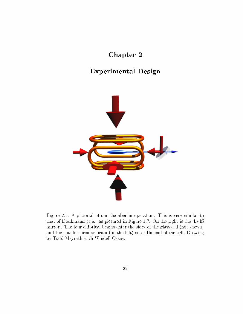
Figure 2.1: A pictorial of our chamber in operation. This is very similar to

that of Dieckmann et al. as pictured in Figure 1.7. On the right is the `LVISmirror'. The four elliptical beams enter the sides of the glass cell (not shown)and the smaller circular beam (on the left) enter the end of the cell. Drawing

by Todd Meyrath with Windell Oskay.

22

23

2.1 Chamber Design

2.1.1 The Idea

The setup for this experiment is similar in principle to that of the 2D+-MOT

of Dieckmann et al. as described in Section 1.5.3. The cooling is done in a

rectangular glass cell. Four large elliptical beams enter the cell on the sides |

these are MOT beams. A smaller circular beam enters the cell on the end and

another circular beam re ects o� a special mirror and into the glass cell |

these are optical molasses beams. The elliptical MOT beams contain repump

light and the circular optical molasses beams do not. As discussed before, this

leads to an atomic beam that exits the trapping region along the magnetic

�eld axis. The setup is shown pictorially in Figure 2.1. The featured parts of

the vacuum chamber are the `LVIS mirror' and the glass cell.

2.1.2 The Mirror and Glass Cell

The LVIS mirror was fabricated for us by CVI Laser. It is a Zerodur ceramic

glass elliptical mirror blank that has been drilled through with a diamond

core-drill (see Figure 2.2). The hole is of several levels, narrow at the mirror

surface (0:05 inch minor axis) and wide at the rear. This was done primarily

so that the inside of the mirror would not prevent clearance through the hole

in the case of somewhat imperfect orientation of the mirror. The mirror has a

high re ectivity laser line coating at 589 nm. The primary reason we decided

to have a dielectric coating rather than a protected silver coating is that the

metal coating is a `cold coating' and can not be baked (the chamber bake out

is discussed in Section 2.1.4) to more than a modest 125 oC or so, but the

dielectric coating is speci�ed to be bakable to 300 oC. This is not necessarily a

24

Mirror Surface

Figure 2.2: The LVIS mirror. The LVIS mirror is a Zerodur ceramic glasselliptical mirror blank that has been core-drilled and coated with a laser line

dielectric coating at 589 nm. The hole at the mirror surface is elliptical with0:05 inch minor axis. The mirror blank was cut out of a Zerodur rod at 45o.

concern in this test chamber, however, it could be when this setup is installed

on the main chamber. One concern about this dielectric coating was that it

might not preserve the phase di�erence in the s and p polarizations | which

is necessary in order to re ect circular polarization without a change. Such

a problem could potentially be �xed by making the incoming light of the

correct elliptical polarization such that the re ected light would be circular.

This is a phase correction, no amplitude di�erence correction would be needed

since the mirror was a high re ector for all angles of linear polarization. We

learned by testing the mirror prior to its placement in the chamber that it

is insensitive to the polarization | it preserved the phase di�erence between

the s and p light and therefore preserved circular polarization. However, after

25

the chamber bakeout procedure, we noticed that the mirror's properties had

changed. The mirror became, in e�ect, a polarizing beam splitter. Because of

this, we were forced to use a lin ? lin con�guration (that is, the pair of beams

with perpendicular linear polarization) for the optical molasses beams instead

of circular polarizations. To be certain that we had not been in error when

testing the mirror prior to the bake, we re-tested an identical mirror (that was

coated in the same coating run as the mirror in the chamber) and found the

same polarization insensitivity as previously observed.

In designing a mount for the mirror, several things had to be considered:

the mirror was to be in the vacuum chamber (which must be baked) and is

oddly shaped (see Figure 2.2). The mount, shown in Figure 2.3, was machined

out of aluminum. The design is intended to naturally hold an elliptically

shaped mirror. A pair of set screws provide two points of contact. The upper

part of the mirror is pushed by three springs against a pin (a longer set screw)

to provide a third contact point. The springs each sit in a blind hole. The

bottom tip of the mirror sits on a small lip inside the holder. With the mirror

in place and the screws adjusted, the mirror does not touch the inner rim of

the holder. A small amount of pressure will not rock the mirror back and

forth in its place but a more �rm push can move it against the springs. When

baking, the holder and screws expand and the springs provide the expansion

space so that the mirror is not cracked. This holder is mounted on a reducer

ange that has a hole in the center.

The cooling and trapping region is in a rectangular Pyrex cell. The

dimensions of the cell are 1.5 inches by 1.5 inches on the end with a length of

26

setscrews

springs

set screw

Figure 2.3: Aluminum mount that holds the elliptical mirror inside the cham-

ber. The mirror is shown in place on the right. The elliptical mirror rests onthe lower lip and is pushed by two steel set screws. Near the top of the mirror,three tungsten springs push the mirror against another steel screw that is at

45o to the vertical (i.e., parallel to the surface of the mirror). This holds themirror �rmly in place and provides expansion room during the bake to ensure

that the glass mirror substrate is not cracked by the screws or holder.

4 inches. The rectangular glass cell is attached to a tubular glass to metal seal.

The metal is welded to a standard con at (CF) ange that is attached to the

rest of the vacuum chamber. The use of a glass cell provides some advantages

over steel chamber type con�gurations, in particular its compactness. With

such a cell, we have large windows without the bulk of a large windowed steel

piece. The compactness in particular allows magnetic coils to be relatively

close to the trapping region inside the cell enabling high �elds with relatively

low current. Further discussion of the �elds and currents are in Section 2.2.

27

Unfortunately, there are some problems with the cell. The speci�c cell that

we have has very dirty windows | probably residue from the fabrication pro-

cess. Some of the residue was cleaned o� with solvents (including acetone and

methanol) by wiping the inner and outer surfaces with lens tissue. Even after

extensive cleaning, the windows still scatter much light due to the residue.

Another problem of which we have become aware (from experiences with the

main sodium experiment's Pyrex cell) is the fact that Pyrex windows tend to

degrade in the presence of sodium. The degradation shows up in the form of

greater scattering in the windows over time (and consequently loss of power

from the beams) and possibly polarization changes. The exact e�ects are un-

clear as are the processes involved. However, we expect that replacing the

Pyrex cell with a clean fused silica cell will improve the performance.

2.1.3 Vacuum Chamber Setup

The vacuum chamber includes the mirror and glass cell as discussed in the

previous section along with other elements such as a valve and Varian StarCell

ion pump. The chamber is shown in Figure 2.4. In the upper part of the

chamber there is the glass cell that is attached to a custom steel cross. This

custom piece has a small tube that goes to the pinch-o� section that holds an

ampoule of sodium. Opposite the glass cell, the custom cross has a zero length

arm. The reducer ange to which the mirror holder is attached is connected at

this location. It is rotated so that the mirror faces upwards through a window

directly above it. A pair of windows face perpendicular to the plane of the

paper in Figure 2.4a through which one can see the side of the mirror. These

ports are to be used for a plug beam that will be discussed in Section 3.3.

28

I Ions

Star Cell

Star Cell

b)

a)

glass cell

glass cell

detection chamber

customcross

ion pump

ion pump

valve

valve

detectionchamber

customcross

pinch-off (b)

pinch-off (a)

iongauge

ion gauge

Figure 2.4: Chamber setup: a) side view: The glass cell is on the left. Thepinch-o� tube (a) contains the sodium. b) top view: The pinch-o� tube (b)

was used as the pump out port during bake out.

Beyond the reducer ange is a conical enlarger that attaches to the detection

chamber. The detection chamber is a cross with three windows. The part of

the optical molasses beam that passes through the hole in the LVIS mirror

exits the facing window. A detection beam is passed through the pair of

facing windows. Unfortunately, due to an oversight, we did not have another

window to conveniently collect uorescence. We, therefore, had to use the

beam-splitter setup as discussed in Chapter 3. The remainder of the chamber

consists of Bayard-Alpert type ion gauge to measure the pressure as well as

29

a Varian StarCell ion pump (discussed in Appendix A). A valve is located

between the pump and the main part of the chamber that may be used to

choke o� the pump in order to allow for higher pressures in the chamber if

that becomes desirable.

2.1.4 Chamber Bake

The reason for baking the vacuum chamber is to remove water, hydrocarbons,

and other contaminants from the chamber walls. During this process, the

chamber is connected to a portable vacuum pumping station (which we call the

turbo station) through the pinch-o� tube in Figure 2.4b. The station (designed

by Dan Steck) consists of a mechanical roughing pump and a turbomolecular

pump (discussed in Appendix A) that pump the chamber gas load during

the bake. The station also has protection electronics to turn o� the turbo

pump in the event of a large leak or other such problem during the bake. We

baked the vacuum chamber twice. The �rst bake was to approximately 300 oC

and the second to 225 oC. These temperatures are well within speci�cations

for the parts. The �rst bake (without the glass cell or the Zerodur mirror),

was primarily to make sure that the aluminum mirror holder was clean. The

second, and �nal, bake was of the entire chamber. At the end of the second

bake, the ion pump and the ion gauge were turned on brie y ( ashed on).

This was to clean them and allow the emitted particles to be removed from

the system through the turbo pump. At that point in the process with the

ion pump and the turbo pump running, the pressure in the chamber was

2:0� 10�8 torr at room temperature. The chamber was then pinched-o� from

the turbo station to become an independent system. The process of pinching-

30

o� is a simple. The copper tube is pinched by a special device. The device

is consists of two very at steel jaws that move parallel. The jaws squeeze

the upper and lower halves of the copper tube together and the clean surfaces

cold-weld. After pinching-o�, the ion pump brought the chamber pressure

down to 1:7� 10�9 torr. The ion pump operates continuously thereafter.

2.2 Io�e Fields

2.2.1 Field of an In�nite Line Current

The �eld of an in�nite line current is well known [13] to have magnitude

jBlinej =�0I

2�r; (2.1)

where r =px2 + y2 is the distance from the wire. In terms of a vector �eld

we have

Bline(x; y) =�0I

2�

��y

x2 + y2x+

x

x2 + y2y

�; (2.2)

where I = I z and x, y, and z are perpendicular unit vectors.

d

y

x

I

Figure 2.5: The ideal Io�e con�guration consists of four in�nite equal line

currents represented by the large arrows.

31

Figure 2.6: A vector �eld plot of BIo�e in the region between the four wires as

in Equation (2.3).

2.2.2 Simple Calculations on Ideal Io�e Con�guration

The ideal Io�e con�guration consists of four in�nite line currents of equal

magnitude I and delta function thickness (see Figure 2.5). The resultant �eld

is the vector sum of the single �elds as in Equation 2.2:

BIo�e = Bline(x� d=2; y � d=2)�Bline(x� d=2; y + d=2)

+Bline(x+ d=2; y + d=2)�Bline(x + d=2; y � d=2):(2.3)

A vector �eld plot of BIo�e is in Figure 2.6. Note, of course, that in this ideal

case there is no z dependence and this solution can be translated along the

z-axis. The magnitude, BIo�e, can be found to be

BIo�e =pBIo�e �BIo�e

=4�0I

�d2

vuut x2 + y2

1 +�x2+y2

d2

�4+ 8�x4�6x2y2+y4

d4

� (2.4)

32

-0.4 -0.2 0 0.2 0.4

-0.4

-0.2

0

0.2

0.4

y/d

x/d

Figure 2.7: Contour plot of �eld magnitude in the region between the fourwires as in Equation (2.4).

and is shown in Figure 2.7. Near the trap center (i.e., jxj=d; jyj=d � 1), we

can approximate the second two terms in the denominator of the square root

to be much less then one. Then we have an approximate linear dependent �eld

magnitude given by

(BIo�e)0�=

4�0I

�d2r: (2.5)

The approximate �eld gradient near the center of the trap is then

Gm�=

4�0I

�d2; (2.6)

as in Equation (1.9). This can be used to estimate the currents needed for

particular �eld gradients or to determine the gradient produced by particular

values of current.

33

The �eld gradient is important for MOT operation, but another factor

to consider is alignment of the atomic beam axis to the hole in the mirror. By

changing the relative currents in the Io�e wires, one may shift the magnetic

�eld axis. This of course will also skew the �eld from the straight line gradient

above by a small amount which we will neglect. Consider Equation (2.3) at

y = 0 with possibly di�erent currents: In where n = 1; 2; 3; 4:

B0Io�e(x; I1; I2; I3; I4) =Bline(x� d=2;�d=2; I1 + I4)

�Bline(x� d=2;+d=2; I1 + I2)

+Bline(x + d=2;+d=2; I2 + I3)

�Bline(x+ d=2;�d=2; I3 + I4);

(2.7)

where Bline = Bline(x; y; I) as in Equation (2.2). Now, suppose we �x currents

2 through 4 and call them I0 (i.e., I0 = I2 = I3 = I4) and vary I1. We expect

to see a shift in the zero of the �eld along the x axis. The position of zero �eld

along the the x axis (call it x0) is a solution to

[B0Io�e(x; I1; I0; I0; I0) � x]x=x0 = 0: (2.8)

This equation can be solved with result:

x�0 = d�(I1 + 3I0)�

p�I21 + 10I1I0 + 7I20

2(I1 � I0); (2.9)

where x+0 is the solution in the vicinity of the origin. This could also be written

in terms of �I de�ned by I1 � I0 +�I :

x+0 = d�(�I + 4I0) +

p16I20 + 8I0�I ��2

I

2�I

: (2.10)

The formulas of this section can be used for practical estimates of the �elds

for some situations. A discussion about the actual design of the coils used to

34

produce these �elds follows in Section 2.2.3. That discussion will make clear

the choice of writing sums of currents in Equation (2.7). In Section 2.2.4 there

is a discussion about actual measurements of the coils in operation and how

they compare to this theory.

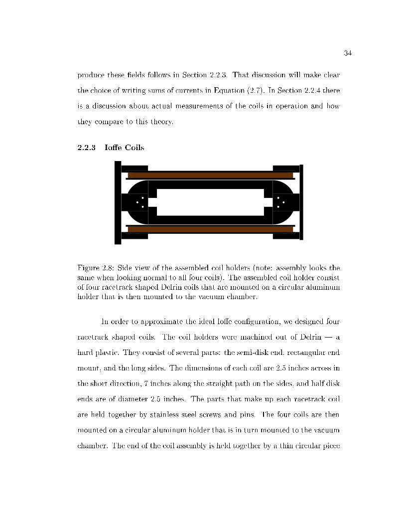
2.2.3 Io�e Coils

Figure 2.8: Side view of the assembled coil holders (note: assembly looks the

same when looking normal to all four coils). The assembled coil holder consistof four racetrack shaped Delrin coils that are mounted on a circular aluminumholder that is then mounted to the vacuum chamber.

In order to approximate the ideal Io�e con�guration, we designed four

racetrack shaped coils. The coil holders were machined out of Delrin | a

hard plastic. They consist of several parts: the semi-disk end, rectangular end

mount, and the long sides. The dimensions of each coil are 2.5 inches across in

the short direction, 7 inches along the straight path on the sides, and half disk

ends are of diameter 2.5 inches. The parts that make up each racetrack coil

are held together by stainless steel screws and pins. The four coils are then

mounted on a circular aluminum holder that is in turn mounted to the vacuum

chamber. The end of the coil assembly is held together by a thin circular piece

35

Figure 2.9: Photo of the coils in the setup. In the center one can see theglass cell surrounded by the black Delrin racetrack shaped Io�e coils. They

are wrapped with red magnetic wire. The coil assembly ends with a Delrinretaining ring for stability. Above and to the sides of the the coil assembly one

can see the 3 inch lenses that are the objectives for the four large telescopesdiscussed in Section 2.4.1.

of Delrin. Figure 2.8 shows the side view of the assembly and Figure 2.9 is a

photo of the coils in the optical table setup. The coil assembly is very strong,

stable, and light weight. Gauge 24 magnet wire was wrapped around each of

the four coils for 200 turns. The wire was wrapped in the counter clockwise

direction (as looked on from the outer side when assembled) from white to

grey connector wires. When hooked up to the current source electronics, care

is taken so that each pair of adjacent wires has current in the same direction.

Each of these pairs of 200 wires then makes up one of the Io�e wires (hence

why we wrote sums of currents in Equation (2.7)).

36

2.2.4 Field Measurements

We made measurements of the magnetic �elds with a Bell Series 9350 Gauss-

meter. The probe was mounted on an XYZ translation stage where the z axis

could easily be found as the location where the x and y components of the

�eld vanish and remain zero for a translation along the z axis. The measure-

ments described here were made along the x axis with y = 0 (it is noted that

measurements along the y axis produced similar results).

The �rst thing that we are interested in is the magnetic �eld gradient

Gm as in Equation (1.9). The theoretical value of Gm is given by Equation

(2.6):

Gm =4�0I

�d2: (2.6)

We note that the formulas from Section 2.2.2 are for the ideal Io�e case. That

case is where the wires are in�nitely long and are of negligible thickness. In

the region of interest, these conditions are fairly well approximated. One point

about the size of the wires is raised that they consist of 400 turns of small wire

on two separate holders (i.e., the sides of two adjacent coils next to each other).

In this approximation, it is not totally clear what value to use for d (the d

in Figure 2.5) since the model assumes the wires are of negligible thickness.

From the mechanical drawings a value of 60mm to 70mm is likely. For the

purpose of estimation of current requirements for construction of electronics

(Section 2.3), we used d = 65mm. Field measurements were made along the

x axis within a few millimeters of the zero �eld location. The results of these

measurements for current I = 0:5A and I = 0:8A appear in Figure 2.10. The

37

−1.5 −1 −0.5 0 0.5 1 1.5−1.5

−1

−0.5

0

0.5

1

1.5

x co

mpo

nent

of m

agne

tic fi

eld

(Gau

ss)

position (mm)

Figure 2.10: Measured magnetic �eld near center zero �eld line. This mea-surement was done in the x direction where the y and z components are zero.

The dashed line is for current I = 0:5A in all coils. The solid line is for currentI = 0:8A in all coils. The crosses mark the data points which have error less

then �0:01G. It is noted that the sets of data form straight lines as expectedfrom theory. The magnetic �eld gradients are Gm(I = 0:5A) = 6:75G=cmand Gm(I = 0:8A) = 10:4G=cm, respectively.

measured values �t straight lines very well. From the measured values we can

determine Gm for the respective current, �nding an average Gm as

hGmi =1

N

NXn=1

B(xn)

xn; (2.11)

where f(xn; B(xn))g is the set of data points. Measurements give magnetic

�eld gradients of hGmi(I = 0:5A) = 6:75G=cm and hGmi(I = 0:8A) =

10:4G=cm, respectively. If we assume Equation (2.6) is valid, then we can

determine d for those currents: d(I = 0:5A) = 68:8mm and d(I = 0:8A) =

70:2mm with average hdi = 69:5mm. If we use this as a reasonable estimate

38

0.4 0.45 0.5 0.55 0.6−2

−1.5

−1

−0.5

0

0.5

1

1.5

2

coil 1 current (A)

chan

ge in

zer

o po

sitio

n (m

m)

Figure 2.11: This plot shows the change in the zero position of the magnetic�eld in the x direction for a change of current in coil 1. Coils 2 to 4 havecurrent I = 0:5A. The dotted line is for measured values and the solid line is

theory (Equation (2.10) with d = 69:5mm and I0 = 0:5A).

of d and assume Equation (2.6) then we have

Gm�=

�13:25

G

cm � A

�I: (2.12)

In addition to gradient measurements, we also considered the shift of

the zero in the magnetic �eld along one axis for di�erent currents. Plots of

the results appear in Figure 2.11 and Figure 2.12 for di�erent currents. Like

the previous measurements, these were made along the x axis. The error bars

for these measurements are much greater due to the lack of resolution on the

current control electronics readout | which could potentially be improved.

The plots, however, show reasonable agreement with the theory in Equation

39

0.7 0.75 0.8 0.85 0.9−1.5

−1

−0.5

0

0.5

1

1.5

coil 1 current (A)

chan

ge in

zer

o po

sitio

n (m

m)

Figure 2.12: This plot shows the change in the zero position of the magnetic�eld in the x direction for a change of current in coil 1. Coils 2 to 4 havecurrent I = 0:8A. The dotted line is for measured values and the solid line is

theory (Equation (2.10) with d = 69:5mm and I0 = 0:8A).

(2.10):

x+0 = d�(�I + 4I0) +

p16I20 + 8I0�I ��2

I

2�I

: (2.10)

We can see that the zero position can be shifted by several millimeters for

some 100mA of current di�erence. Equation (2.10), using value d = 69:5mm,

can be used to estimate this shift.

2.3 Current Control Electronics

The purpose of these electronics is to provide a stable and independent current

source for each of the four coils described in Section 2.2.3. Estimates of the

current requirements for reasonable �eld gradients come from the coil design

40

and the theory of Section 2.2.2. The electronics described here can reliably

supply well over 2A of current to each coil. Of course, with currents over an

Amp and a half or so overheating of the coils could be a problem. The elec-

tronics are also designed to provide a few options for control of these currents

(i.e., interface options for the current box). The circuit consists of two parts:

the power circuit and the control circuit. They will be described in this section

[14, 15].

2.3.1 Power Circuit

Figure 2.13 shows the power circuit that drives the MOT coils. The key to

the circuit is the IRF620. It is a power MOSFET by International Recti�er

which can have up to 5:2A of continuous drain current. It is a TO-220 type

package and is attached to a heat sink with a thermo-pad for heat transfer

and electrical isolation.

The part of the circuit that is in parallel with the coil is a type of

\snubber" to suppress the inductive kick. This speci�c con�guration was cho-

sen because it gives a linear decay of the current in the coil. This is as opposed

to a more typical con�guration of a diode (such as the MR752 in Figure 2.13)

with a resistor which would have a long exponential tail. For the circuit shown

here in Figure 2.13, when the FET is suddenly turned o�, we have

LdI

dt+ V = 0; (2.13)

where L is the inductance of the coil load and V is the sum of the other voltage

drops (zener, transistor, and diode). So, we have

I(t) = I0 �V

Lt; (2.14)

41

Figure 2.13: Power circuit. Current is controlled by the FET, the \snubber"part of the circuit is to limit the inductive kick and provide a fast shuto� of

the �eld.

which, of course, is only the case when the transistor (2N6059) is turned on

(i.e., when the voltage across the zener is the zener voltage). So, as the current

is close to zero, it would not be surprising to see small oscillations in the �eld.

This setup is useful in situations where fast turn o� is important and could

be potentially optimized for temporal requirements with a choice of the zener

diode, transistor, etc. for the particular inductive load that is used. For

application in this experiment, however, fast turn o� is not needed since the

coils are to be operated with constant current. The snubber is also needed,

of course, to prevent inductive kick from destroying the electronics. All of the

components of the power circuit are mounted on a large heat sink that is air

cooled.

42

One point of caution when operating this circuit is that although the

maximum current through the IRF620 is around 5A, the maximum power is

Pmax = 50W. The power supply voltage drops over the coils and the IRF620

(ignore the 0:1 resistor). Therefore, the supply voltage, Vsupply, should be

chosen for the coil resistance, Rcoil, and the circuit should operate with a

current, I, that satis�es the inequality:

IVFET = I(Vsupply � RcoilI) � 50W: (2.15)

In the case of our coils, with resistance of about 9:5, we use a supply voltage

of +28V. In this case, the maximum power through the FET is about 20W

at about I = 1:5A. With a +28V supply, the max current is a little less the

3A | this is when there is no voltage drop across the FET (and the current

is not regulated). So with this setup there is no concern that the FET will

burn out. However, as the author learned the hard way, a smaller test load

in place of the coils can easy cause burn out the FET. For example, with the

+28V supply a minimum load of 5 should be used to keep the maximum

FET power at around 40W (well below Pmax = 50W).

2.3.2 Control Circuit

The control circuit is closely based on the design by Martin Fischer. It consists

of a feedback loop with the voltage across the 0:1 power resistor as a sense

and the FET gate voltage as the control. The circuit is shown in Figure

2.14. There are several controls that can modulate the current, they are: front

panel pot, external input, and TTL input. How this control circuit works can

be understood by looking at a simpli�ed general example as in Figure 2.15.

43

Figure 2.14: Current control circuit (based on design by Martin Fischer).Feedback loop with the power circuit controls the current in the coil.

Considering the case of the ideal opamp (i.e., in�nite input impedance and

equality of the input voltages), we can see that the output voltage is given by

VO =

�1 +

ZF

ZE

+ZF

ZS

�VP +

ZF

ZE

VE �ZF

ZS

VS; (2.16)

where VE (the external input) is negative because of the inverting ampli�er

UA3 in Figure 2.14. VS is the voltage feedback sense. The output voltage

(and hence the current since the the power FET gate is at this voltage) is

44

V

V

S

EE

SV

Z

Z

FZ

P

O

-V

Figure 2.15: Simpli�ed general example of the control circuit operation.

controlled by the external input and by the front panel pot (by setting VP).

The TTL signal controls the analog switches DG201 in Figure 2.14. In

this way, a high TTL signal is required to have current in the coils. One could,

for instance, modulate the current by the TTL signal.

Figure 2.16: Stable voltage reference for control circuit in Figure 2.14. TheLM399 package is a temperature stabilized zener diode which serves as the

reference voltage of about 7V.

A high precision voltage reference (LM399) is used for the important

pots in the circuit. The LM399 package is a temperature stabilized zener diode

45

which serves as the reference voltage of about 7V.

The control circuit and the voltage reference circuit for each channel

were put on an etched copper circuit board. Discussion and drawings of these

boards are in Appendix B.

Monitors of the current are a BNC front panel output and a LCD

package. The LCD package is the DP-654 from Keithley Instruments. It

is a convenient device which is essentially a voltmeter. It has a built-in A/D

converter and a liquid crystal display. A small board is mounted on the LCD to

serve the simple purpose of supplying the correct voltage to the LCD package

from the voltage rails in the box. A photo of the box is shown in Figure B.1

in Appendix B.

2.4 Optical Setup

2.4.1 Large Elliptical Beam Concerns

Since, in this setup, we require large elliptical beams (about 48mmwaist diam-

eter major axis and 16mm minor), we require large optics for beam expanding

telescopes. From the cost perspective, large cylindrical lenses are impractical,

so we decided to use an anamorphic prism pair to make the beam elliptical

when it is small and use a spherical telescope. The anamorphic prism pair is a

convenient package that expands the beam 3� in one direction only. Since the

�nal beam size (major axis) is around 2 inch waist, we decided to use 3 inch

objectives to avoid fringes as the result of beam clipping.

Another important feature of the beams is the circular polarization.

Normally, in a situation with small beams, one keeps linear polarization until

46

right before entering the MOT chamber so that the quarter-wave plate is the

last optic. That way one avoids polarization problems due to birefringence in

dielectric mirrors, etc. The problem here, again, is the size of the beams | the

cost of a 3 inch quarter-wave plate is painful to talk about, especially when 4

would be needed. Our solution to this problem is to use a small quarter wave

plate and place it near the focus of the telescope. There the wavefront most

resembles a plane wave. In this setup the objective of the telescope is then the

�nal optic.

2.4.2 Laser and Practical Table Setup Concerns

Since this experiment is running in parallel with the main experiment (to which

it is intended to become part), optical table space is limited. Using a di�erent

table is unrealistic because of the need for the dye-laser setup complete with

frequency locking and modulators. So we built a level over the present optics.

This simply consists of a large aluminum plate supported by stainless steel

posts. Large holes in the plate were cut to allow MOT beam and repump beam

to be periscoped up to the second level. On the main level, the lower periscope

mirrors are placed on kinematic mounts so that they could be removed and

replaced very easily. The optics for the horizontal beams are put on three very

small third levels. Vertical optics are mounted on large steel posts.

2.4.3 Optical Setup

Most of the horizontal optical setup is shown in Figure 2.17. Two beams are

brought up from the table below: the MOT beam and the repump beam. The

MOT beam is linearly polarized (normal to the plane of the paper initially).

47

The upper periscope mirrors are labeled in Figure 2.17. The MOT beam passes

through a 1=2{wave plate and then through a polarizing beamsplitter cube.

The 1=2{wave plate is used to select the intensity balance between the large

elliptical beams (the light that passes through the cube) and the small circular

beams (the light that re ects from the cube). The light that re ects from the

cube goes through a telescope to a �nal size of approximately 8mm waist and

then is split. Half the light is directed into the end of the glass cell and the

other half is brought down onto the LVIS mirror and re ected into the cell.

The MOT light that passes through the cube then enters another cube where it

is combined with the repump light. A small amount of the MOT/repump light

is taken by a beamsplitter to be used for the detection beams. The bulk of the

MOT/repump light passes to an anamorphic prism pair where it is expanded

3� in one direction. This small elliptical beam of MOT/repump light is split

at a beamsplitter (located at the end of the coils in Figure 2.17). One half

goes to the vertical telescopes (not shown), the other goes to the horizontal

telescopes.

The major focus in the optical setup revolves around the glass cell and

the beams that enter it. In Section 2.4.1 we discussed some of the concerns of

the large elliptical beams. Because space is limited, especially in the vertical

direction, we choose fast lenses in order to have the telescopes as short as

possible. On one side, the small fast lens in conjunction with the large lens

make a telescope. On the retrore ected side, a mirror is placed at the focus of

the large lens to make a unity magni�cation telescope. Mounting of the pair

of vertical telescopes (one above and one below the glass cell) was done using

90o post clamps to large steel posts (this is not shown in Figure 2.17). The

48

vertical and horizontal telescope setups are the same. Near the focus of each

of the telescopes for the elliptical beams is a 1=4{wave plate positioned to give

the correct circular polarization.

49

I Ions

Star Cell

����

����

New

port KPX

109

2501/

2 W

P

Ana.PrismPair

Newport KPX079

38.1

AO

M

Melles G

riot 01LPX

223 Mel

les

Gri

ot 0

1LPX

223

New

port KPX

076

MOTBeam

repump

75

PMT

75

Figure 2.17: Optics setup. See Section 2.4.3 for discussion.

50

Figure 2.18: Photo of optical setup. This is a photograph of the experiment

at some mid-point of the setup.

Chapter 3

Detection, Observations, Conclusions

3.1 Detection Estimates

In an optimized setup, we might hope for atomic ux on the order of 108 s�1

(experiments of other groups [1, 2, 3] had similar or larger uxs). Suppose

the atoms are moving in a beam with velocity 10m=s. With a 1 cm detection

beam of resonant light above saturation intensity there would be uorescence of

order 1�W is all directions. Of course, in order for the setup to be optimized

we need to be able to detect the atomic ux and maximize it by adjusting

the magnetic �eld axis and the molasses beams. Therefore, initially, we are

required to detect much weaker intensity. Furthermore, we are only able to

collect some fraction of the uorescent light onto a detector. More realistically,

we are required to be able to detect light on the order of 1 nW. This light level

is diÆcult to see by eye and impossible for a photodiode, so we use a photo-

multiplier tube (PMT).

One problem with our setup is the oversight in the construction of the

chamber where a window to be used exclusively for the PMT was not included.

Therefore, we were forced to setup the detection using a beamsplitter cube as

shown in the upper right hand corner of Figure 2.17. This is problematic. In

51

52

addition to losing uorescence intensity through the beamsplitter cube, the

back-re ection of the detection beam must be blocked in order to prevent

saturation of the very sensitive PMT. This can result in a very small signal

above a large background.

In order to detect the atomic beam, we employ a lock-in technique. This

is discussed in Section 3.3. First, we discuss the basics of lock-in ampli�ers.

3.2 Lock-in Ampli�ers

A lock-in ampli�er can be used to detect small AC signals that may be obscured

by noise several orders of magnitude larger than the signal. The lock-in can

be thought of as behaving as a bandpass �lter of very narrow bandwidth. The

�lter is centered at the frequency of the signal and rejects noise at all other

frequencies.

Experiment

Signal

Mod In

S

R

M

PassPLL

Low

V

V

V

DC amp

FunctionGenerator

VO

Lock-in amplifier

AC amp

Figure 3.1: Lock-in ampli�er block diagram.

For more details on the operation of a lock-in ampli�er, we look at the

block diagram in Figure 3.1. We have an experiment with some property that

we can modulate and measure the response. A modulation signal is sent to

53

the experiment and to the lock-in as the reference. The experimental signal is

the input to the lock-in: VS = AS cos(!St+�S), where �S might be phase delay

response of the experiment. The modulation signal is put into a phase locked

loop (PLL) in order to generate a noise-free sinusoid VR = AR cos(!Rt + �R)

with adjustable phase �R. These two signals are then mixed with result:

VM = ARAS cos(!Rt + �R) cos(!St+ �S)

=1

2ARAS(cos[(!R + !S)t+ (�R + �S)]

+ cos[(!R � !S)t+ (�R � �S)]):

(3.1)

The sum of frequency component is removed by the low pass �lter and with

!R = !S we get DC output:

VO =1

2ARASGDC cos(�R � �S); (3.2)

where GDC is the gain in the DC ampli�er. The phase of the experimental

signal �S can then be determined by adding �=2 to the adjusted reference

phase �R that nulls the signal [14, 15, 16].

3.3 Plug and Probe Beams and Time-of-Flight

We set up to do lock-in detection of the atomic beam and time-of- ight mea-

surements as shown in Figure 3.2. The so-called plug beam is MOT light with

repump that enters the vacuum chamber slightly before the LVIS mirror as

described in Section 2.1.3. This beam pushes the atoms o� axis before they

reach the exit aperture | in e�ect, plugging the hole. The intensity of the

plug beam is modulated by a 40MHz AOM. Of course, the AOM also produces

a 40MHz frequency shift to the 20MHz red beam, so we use the blue shifted

order and end up with an intensity modulated beam that is 20MHz blue. A

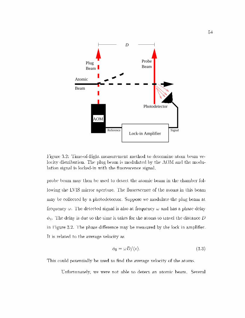
54

Probe

Atomic

Beam

BeamBeamPlug

Photodetector

Lock-in Amplifier

D

AOM

SignalReference

Figure 3.2: Time-of- ight measurement method to determine atom beam ve-locity distribution. The plug beam is modulated by the AOM and the modu-

lation signal is locked-in with the uorescence signal.

probe beam may then be used to detect the atomic beam in the chamber fol-

lowing the LVIS mirror aperture. The uorescence of the atoms in this beam

may be collected by a photodetector. Suppose we modulate the plug beam at

frequency !. The detected signal is also at frequency ! and has a phase delay

�S. The delay is due to the time it takes for the atoms to travel the distance D

in Figure 3.2. The phase di�erence may be measured by the lock-in ampli�er.

It is related to the average velocity as

�S = !D=hvi: (3.3)

This could potentially be used to �nd the average velocity of the atoms.

Unfortunately, we were not able to detect an atomic beam. Several

55

possible problems could lead to this inability. The problem with the glass cell

as discussed in Section 2.1.2 might have prevented the 2D-MOT from working

all together. So, perhaps we never had a beam to detect. Another problem

was the unfortunate circumstance that we did not have a separate viewport

to collect uorescence. Detection was very diÆcult.

3.4 Summary and Conclusions

In this work we have described the design and construction of an experimental

apparatus for a two-dimensional magneto-optical trap. Simple models of laser

cooling and trapping and their relevance were explained in Chapter 1. The

possible application of this setup is as a low velocity atomic beam source for

loading atom traps.

We discussed in some detail the design of the apparatus and consid-

erations in Chapter 2. In particular, the mirror that is mounted inside the

chamber and the magnetic coils are important for the setup. Many details of

the optics are found in Section 2.4.

Some parts that were designed and built for this experiment worked

very well. For example, current control electronics and the Io�e coils have been

trouble-free from design and construction to implementation. The magnetic

�elds were mapped out and agree well with theoretical estimates. The holder

for the mirror inside the chamber also worked as expected | �rmly holding

the mirror in place without cracking it during bake-out.

We talked about a few aspects of the construction of this experiment

that could be improved. The LVIS mirror, as discussed in Section 2.1.2, ap-

56

parently changed properties during the chamber bake. Perhaps a mirror with

a di�erent coating or a protected metal mirror would work better. The Pyrex

cell, discussed in the same section, has problems of scattering light from the

windows. A better constructed cell would hopefully avoid these problems as

well as those of previous Pyrex cells as pointed out in Section 2.1.2. Finally,

another window on the detection chamber would greatly simplify the detection

setup.

Appendix

57

Appendix A

Vacuum Pumps and Gauges

The chamber (as discussed in Section 2.1) has an ion pump and an ionization

gauge. The turbo station used in the chamber bake process has a mechani-

cal roughing pump, a turbo pump (hence the station name), a thermocouple

gauge, and an ionization gauge.

Thermocouple gauges are useful for measuring pressure in the range of

about 1 torr to 10�3 torr. The gauge consists of a thermocouple measuring the

temperature of a heated �lament. The temperature depends on the rate of heat

loss to the surrounding gas (i.e. on thermal conductivity). This dependence is

nonlinear and the manufacturer generally calibrates the gauges and controllers

for air.

Ion gauges are lower pressure devices than thermocouple gauges. They

may be used in pressure range of 10�3 torr to 10�10 torr. These gauges op-

erate by measuring ion current. Electron impact near the gauge ionizes gas

particles. The positive ions are then collected at a negative electrode | this

is the ion current that is measured. This current is linear with pressure but

obviously dependent on the gas present. Standard devices are calibrated for

air. Interestingly, ion gauges have a small side e�ect of being slow pumps.

58

59

This is because the ionized particles collected at the electrode are removed

from the system.

The pumps on the turbo station are both mechanical pumps. The

standard roughing pump is rotary pump that is oil-sealed. These pumps are

useful to down to the militorr range. As the name implies, such a pump may

be used to `rough pump' the system down from atmospheric pressure. Far

more impressive then the roughing pump is the turbo pump. This pump is

also a mechanical pump and is run in series with the roughing pump. In this

setup, the roughing pump is true to it's name and pumps through the non-

operating turbo pump to rough down the system. After the turbo pump is

turned on, the roughing pump works as a backing pump. The turbo pump can

be visualized as a fan | but running at 75; 000 rpm! Particles in the chamber

get a signi�cant mechanical kick towards the backing pump. In e�ect, the

turbo pump is able to hold a pressure di�erence of 5 to 6 orders of magnitude.

This was the device that did the signi�cant pumping during the bakes.

The ion pump operates similar to the side e�ect pumping of the ion

gauge. The pump consists of a stainless-steel anode and a titanium cathode

between which there is a magnetically con�ned discharge. Neutral gas from

the chamber is ionized and slams into the titanium cathode removing it from

the system. Our pump is a Varian StarCell. It operates at 5; 000Volts and

has a pumping speed of 20 L=s. [15]

Appendix B

Control Circuit Board Layouts

This appendix gives the layouts for the etched boards for the circuits described

in Section 2.3. The board layouts were done in EAGLE (Easily Applicable

Graphics Layout Editor) from CadSoft. The drawings for the boards were then

printed on transparencies with a high resolution laser printer. Boards have a

copper layer covered by a photo resist coating. Exposure with a uorescent

lamp for 8 to 10 minutes is suÆcient for developing. The developed board

may then be etched with ferric chloride solution. The etching uid produces

�ne circuit boards.

Figure B.1: Photo of the electronics box. Near the front panel are four control

circuit boards. On the large heat sinks in the rear of the box are the powercircuits.

60

61

Figure B.2: Control circuit board layout (done in EAGLE by Todd Meyrath).

This board has both the control circuit of Figure 2.14 and the voltage reference

circuit as in Figure 2.16.

62

Figure B.3: Circuit for the panel LCD.

Figure B.4: Circuit board layout for the LCD (done in EAGLE by ToddMeyrath). This board serves the simple purpose of supplying the correct

supply voltage to the LCD package from the voltage rails in the box. It is

mounted on the LCD on the front panel.

Bibliography

[1] K. Dieckmann, R.J.C. Spreeuw, M. Weidem�uller, and K. T. M. Walraven:

\Two-dimensional magneto-optical trap as a source of slow atoms;" Phys-

ical Review A, Vol. 58, No. 5, pp. 3891-3895; 1998.

[2] Z.T. Lu, K.L. Corwin, M.J. Renn, M.H. Anderson, E.A. Cornell, and C.E.

Wieman: \Low-Velocity Intense Source of Atoms from a Magneto-optical

Trap;" Physical Review Letters, Vol. 77, pp. 3331-3334; 1996.

[3] C.Y. Park, M.S. Jun, and D. Cho: \Magneto-optical trap loaded from a

low-velocity instense source" Journal of The Optical Society of America

B, Vol. 16, No. 6, pp. 994-997; June 1999.

[4] Dieter Suter: \The Physics of Laser-Atom Interactions;" Cambridge Uni-

versity Press, New York, 1997.

[5] H.J. Metcalf and P. van der Straten: \Laser cooling and Trapping;"

Springer, New York; 1999.

[6] W.D. Philips: \Laser Cooling and Trapping of Neutral Atoms;" in Laser

Manipulation of Atoms and Ions Proceedings of the International School

of Physics \Enrico Fermi," Italian Physical Society pp. 289-343; Elsevier

Scienti�c; 1992.

63

64

[7] E.L. Raab, M. Prentiss, Alex Cable, Steven Chu, D.E. Pritchard: \Trap-

ping of Neutral Sodium Atoms with Radiation Pressure" Physical Review

Letters, Vol. 59, No. 23, pp. 2631-2634; 1987.

[8] J. Dalibard and C. Cohen-Tannoudji: \Laser Cooling Below the Dopper

Limit by Polarization Gradients | Simple Theoretical-Models;" J. Opt.

Soc. Am. B 6, pp. 2023-2045. 1989.

[9] A. M�uck: \Recoil-Induced Resonances for Velocimetry of Cold Cesium

Atoms" Master's Thesis: Department of Physics, University of Texas at

Austin, Austin, Texas. 1999.

[10] D.A. Steck: \Sodium D2 Line Data;" University of Texas at Austin,

Austin, Texas. 2000. www.ph.utexas.edu/~quantopt.

[11] R.C. Weast, editor: \CRC Handbook of Chemistry and Physics, 61st

Edition 1980-1981;" CRC Press, Inc.; Boca Raton, Florida; 1980.

[12] B.H. Bransden and C.J. Joachain: \Physics of Atoms and Molecules;"

Addison Wesley Longman, Essex, England, 1983.

[13] D.J. GriÆths: \Introduction to Electrodynamics" 2nd ed. Prentice Hall,

New Jersey; 1989.

[14] P. Horowitz and W. Hill: \The Art of Electronics" 2nd ed. Cambridge

University Press, New York; 1989.

[15] J.H. Moore, C.C. Davis, and M.A. Coplan: \Building Scienti�c Appara-

tus: A Practical Guide to Design and Construction" 2nd ed. Addison-

Wesley; Reading, Massachusetts; 1989.

65

[16] Stanford Research Systems: \Model SR510 Lock-In Ampli�er Manual;"

SRS, Inc. Sunnyvale, California. 1989.

Vita

Todd Philip Meyrath was born on August 1, 1975 in Rochester, New York as

the son of Frank and Donna Meyrath. He attended Clarke Central High School

in Athens, Georgia. In 1998, he was awarded Bachelor of Science in Physics

and Bachelor of Science in Applied Mathematics degrees from The Georgia

Institute of Technology. He entered The Graduate School of The University

of Texas at Austin in August 1998.

Permanent address: 255 Selkirk Ln.

Duluth, Georgia 30097

This thesis was typeset with LATEXz by the author.

zLATEX is a document preparation system developed by Leslie Lamport as a special

version of Donald Knuth's TEX Program.

66